Ilmanlaadun julkaisujaPublikationer om luftkvalitetPublications on air quality

No. 31

DETECTING TRENDS OF ANNUAL VALUES OF

ATMOSPHERIC POLLUTANTS BY THE MANN-KENDALL

TEST AND SEN’S SLOPE ESTIMATES

-THE EXCEL TEMPLATE APPLICATION MAKESENS

Timo SalmiAnu MäättäPia AnttilaTuija Ruoho-AirolaToni Amnell

Ilmatieteen laitosMeteorologiska InstitutetFinnish Meteorological Institute

Helsinki 2002

ISBN 951-697-563-1ISSN 1456-789X

Painopaikka:Edita Oyj

Helsinki 2002

Series title, number and report code of publicationPublished by Finnish Meteorological Institute Publications on Air Quality No. 31

Vuorikatu 24, P.O. Box 503 Report code FMI-AQ-31FIN-00101 Helsinki, Finland Date August 2002

Authors Name of project Air Quality Assessment inTimo Salmi, Anu Määttä, Pia Anttila, the Baltic countries as a consequence ofTuija Ruoho-Airola and Toni Amnell local pollution and long range transport

- a co-operation between Nordic andBaltic countries within the frameworkof the EMEP’s 20 years Assessment

Commissioned by Nordic Council of MinistersTitleDetecting trends of annual values of atmospheric pollutants by the Mann-Kendall test andSen’s slope estimates –the Excel template application MAKESENS

Abstract

An Excel template – MAKESENS – is developed for detecting and estimating trends in thetime series of annual values of atmospheric and precipitation concentrations. The procedureis based on the nonparametric Mann-Kendall test for the trend and the nonparametric Sen’smethod for the magnitude of the trend. The Mann-Kendall test is applicable to the detectionof a monotonic trend of a time series with no seasonal or other cycle. The Sen’s methoduses a linear model for the trend. The theory of the calculation, the user’s manual and themacro code are presented. As an example the long term trends of precipitation andatmospheric concentrations of some compounds at the Virolahti air quality monitoringstation of the Finnish Meteorological Institute are calculated and briefly discussed.

Publishing unitFinnish Meteorological Institute, Air Quality ResearchClassification (UDK) Keywords504.064 trend, Mann-Kendall test, Sen’s method,519.234 annual time series, trend significanceISSN and series title1456-789X Publications on Air QualityISBN Language951-697-563-1 EnglishSold by Pages 35 PriceFinnish Meteorological Institute / LibraryP.O.Box 503, FIN-00101 Helsinki NoteFinland

Table of Contents

1 Introduction...................................................................................................................7

2 Calculation of the Mann-Kendall test and the magnitude of the trend with the

Sen’s method in MAKESENS..............................................................................................7

2.1 Mann-Kendall test.......................................................................................................8

2.1.1 Number of data values less than 10 ....................................................................8

2.1.2 Number of data values 10 or more....................................................................10

2.2 Sen’s method.............................................................................................................11

3 User’s manual for MAKESENS ................................................................................12

3.1 Entering the time series and other input values ........................................................13

3.2 Summary table of results ..........................................................................................16

3.3 Visual viewing of data and results ............................................................................19

4 Examples......................................................................................................................21

5 Summary......................................................................................................................24

6 References....................................................................................................................25

7 Appendix 1. The macro code of MAKESENS..........................................................26

7

1 Introduction

An Excel template MAKESENS (Mann-Kendall test for trend and Sen’s slope estimates) is

developed for detecting and estimating trends in the time series of the annual values of

atmospheric and precipitation concentrations. The need for this kind of simple and easy- to-

use tool came up in the research project ”Air quality Assessment in the Baltic countries as a

consequence of local pollution and long range transport - a co-operation between Nordic

and Baltic countries within the framework of EMEP’s 20-years Assessment” financed by

the Nordic Council of Ministers. This subproject is a contribution to the EMEP’s

(Evaluation of the Long-Range Transmission of Air Pollutants in Europe) twenty years of

assessment work initiated by the EMEP’s Task Force on Measurements and Modelling in

Vienna October 2000 (TFMM 2000). This European-wide effort will assess the outcome of

the emission control measures in Europe between 1980-2000, focusing on the significance

of changes in concentrations and deposition in relation to emission changes.

The calculation of the Mann-Kendall test and the nonparametric Sen’s method are briefly

described here. We also present a detailed user’s manual of MAKESENS, its macro code

and some examples. In addition to the statistical calculations, MAKESENS also provides a

simple graphical interface to assist the visual inspection of the time series and the statistical

results. The details of the theories can be found in Gilbert (1987). Also Sirois (1998) gives

an educative summary of the application of these methods in atmospheric chemistry

studies.

2 Calculation of the Mann-Kendall test and the magnitude of the trend

with the Sen’s method in MAKESENS

MAKESENS performs two types of statistical analyses. First the presence of a monotonic

increasing or decreasing trend is tested with the nonparametric Mann-Kendall test and

8

secondly the slope of a linear trend is estimated with the nonparametric Sen’s method

(Gilbert 1987). These methods are here used in their basic forms; the Mann-Kendall test is

suitable for cases where the trend may be assumed to be monotonic and thus no seasonal or

other cycle is present in the data. The Sen’s method uses a linear model to estimate the

slope of the trend and the variance of the residuals should be constant in time. These

methods offer many advantages that have made them useful in analysing atmospheric

chemistry data. Missing values are allowed and the data need not conform to any particular

distribution. Besides, the Sen’s method is not greatly affected by single data errors or

outliers.

2.1 Mann-Kendall test

The Mann-Kendall test is applicable in cases when the data values xi of a time series can be

assumed to obey the model

iii tfx ε+= )( , (1)

where f(t) is a continuous monotonic increasing or decreasing function of time and the

residuals εi can be assumed to be from the same distribution with zero mean. It is therefore

assumed that the variance of the distribution is constant in time.

We want to test the null hypothesis of no trend, Ho, i.e. the observations xi are randomly

ordered in time, against the alternative hypothesis, H1, where there is an increasing or

decreasing monotonic trend. In the computation of this statistical test MAKESENS exploits

both the so called S statistics given in Gilbert (1987) and the normal approximation (Z

statistics). For time series with less than 10 data points the S test is used, and for time series

with 10 or more data points the normal approximation is used.

2.1.1 Number of data values less than 10

The number of annual values in the studied data series is denoted by n. Missing values are

allowed and n can thus be smaller than the number of years in the studied time series.

9

The Mann-Kendall test statistic S is calculated using the formula

),sgn(1

1 1k

n

k

n

kjj xxS −=� �

−

= +=

(2)

where xj and xk are the annual values in years j and k, j > k, respectively, and

��

��

�

<−−=−>−

=−010001

)sgn(

kj

kj

kj

kj

xxifxxifxxif

xx . (3)

If n is 9 or less, the absolute value of S is compared directly to the theoretical distribution of

S derived by Mann and Kendall (Gilbert, 1987). In MAKESENS the two-tailed test is used

for four different significance levels α : 0.1, 0.05, 0.01 and 0.001. At certain probability

level H0 is rejected in favour of H1 if the absolute value of S equals or exceeds a specified

value Sα/2, where Sα/2 is the smallest S which has the probability less than α/2 to appear in

case of no trend. A positive (negative) value of S indicates an upward (downward) trend.

The minimum values of n with which these four significance levels can be reached are

derived from the probability table for S as follows.

Significance level

αααα

required n

0.1 ≥ 4

0.05 ≥ 5

0.01 ≥ 6

0.001 ≥ 7

10

The significance level 0.001 means that there is a 0.1% probability that the values xi are

from a random distribution and with that probability we make a mistake when rejecting H0

of no trend. Thus the significance level 0.001 means that the existence of a monotonic trend

is very probable. Respectively the significance level 0.1 means that there is a 10%

probability that we make a mistake when rejecting H0.

2.1.2 Number of data values 10 or more

If n is at least 10 the normal approximation test is used. However, if there are several tied

values (i.e. equal values) in the time series, it may reduce the validity of the normal

approximation when the number of data values is close to 10.

First the variance of S is computed by the following equation which takes into account that

ties may be present:

��

���

�+−−+−= �

=

q

pppp tttnnnSVAR

1)52)(1()52)(1(

181)( . (4)

Here q is the number of tied groups and tp is the number of data values in the pth group.

The values of S and VAR(S) are used to compute the test statistic Z as follows

��

�

��

�

�

<+=

>−

=

0)(

100

0)(

1

SifSVAR

SSif

SifSVAR

S

Z (5)

The presence of a statistically significant trend is evaluated using the Z value. A positive

(negative) value of Z indicates an upward (downward) trend. The statistic Z has a normal

distribution. To test for either an upward or downward monotone trend (a two-tailed test) at

α level of significance, H0 is rejected if the absolute value of Z is greater than Z1-α/2, where

11

Z1-α/2 is obtained from the standard normal cumulative distribution tables. In MAKESENS

the tested significance levels α are 0.001, 0.01, 0.05 and 0.1.

2.2 Sen’s method

To estimate the true slope of an existing trend (as change per year) the Sen's nonparametric

method is used. The Sen’s method can be used in cases where the trend can be assumed to

be linear. This means that f(t) in equation (1) is equal to

f(t) = Qt + B (6)

where Q is the slope and B is a constant.

To get the slope estimate Q in equation (6) we first calculate the slopes of all data value

pairs

kjxx

Q kji −

−= , (7)

where j>k .

If there are n values xj in the time series we get as many as N = n(n-1)/2 slope estimates Qi.

The Sen’s estimator of slope is the median of these N values of Qi. The N values of Qi are

ranked from the smallest to the largest and the Sen’s estimator is

[ ]2/)1( += NQQ , if N is odd

or (8)

[ ] [ ]( )2/)2(2/21

++= NN QQQ , if N is even.

12

A 100(1-α)% two-sided confidence interval about the slope estimate is obtained by the

nonparametric technique based on the normal distribution. The method is valid for n as

small as 10 unless there are many ties.

The procedure in MAKESENS computes the confidence interval at two different

confidence levels; α = 0.01 and α = 0.05, resulting in two different confidence intervals.

At first we compute

)(21 SVARZC αα −= , (9)

where VAR(S) has been defined in equation (4), and Z1-α/2 is obtained from the standard

normal distribution.

Next M1 = ( N - Cα )/2 and M2 = ( N + Cα )/2 are computed. The lower and upper limits of

the confidence interval, Qmin and Qmax, are the M1th largest and the (M2 +1)th largest of the N

ordered slope estimates Qi. If M1 is not a whole number the lower limit is interpolated.

Correspondingly, if M2 is not a whole number the upper limit is interpolated.

To obtain an estimate of B in equation (6) the n values of differences xi – Qti are calculated.

The median of these values gives an estimate of B (Sirois 1998). The estimates for the

constant B of lines of the 99% and 95% confidence intervals are calculated by a similar

procedure.

3 User’s manual for MAKESENS

The MAKESENS template was created using Microsoft Excel 97 and the macros were

coded with Microsoft Visual Basic. The template consists of four worksheets: About,

Annual data, Trend Statistics and Figure. The About worksheet gives general

information about the template. The data of time series are entered into the Annual data

13

worksheet. The calculation macro can be activated by using the button Calculate Trend

Statistics and the Trend Statistics worksheet contains the results. Finally, the original data

and the statistics can be viewed numerically and visually in the Figure worksheet one time

series at a time.

3.1 Entering the time series and other input values

All the input values are entered in the Annual data worksheet (see Figure 1). The years,

the annual values and the names of the time series have to be typed or copied (Paste

Special/Values) to the fixed places of the worksheet. The cells in the worksheet, in which

the user may enter data have no shading. The other cells are protected and have grey

shading.

� A title to the whole data set can be typed in cell A3 . This title is also shown in

cells ‘Trend Statistics’!A3 and ‘Figure’!B4.

� The names of the time series are entered in cells B13:Z13 starting from the

column B. The maximum number of time series that can be entered is 25. The

names are transposed into the cells ‘Trend Statistics’!A6:A30. The name of the

time series is also shown in cell ´Figure’!C10 and as the title of Y-axis in the

figure.

� Cell A13 is reserved for the column title “Year”.

� From cell A14 downwards the user must enter an increasing and continuous series

of years. The range of the years shall cover all the time series but excess years in

the beginning or at the end are allowed. The number of years is limited to 100 but

can be extended by changing the value of the constant MaxData in the macro code

(Appendix 1).

� The annual values of each time series must be entered below the name of the time

series according to the years in the column A. An empty cell indicates a missing

value. The values of a time series or the entire table of annual data can also be

copied from another table.

14

Figure 1. The input data is entered to the Annual data worksheet of MAKESENS.

15

� The first and the last year to be handled in trend calculation must be entered in

rows 10 and 11, above the names of the time series. Every time series must have its

own starting and ending year. With these rows you can easily define different time

spans for the trend statistics calculation of each time series. The starting and ending

years are also shown in the cells ‘Trend Statistics’!B6:C30, and in ‘Figure’!C11.

� The number of values of each time series which are selected to trend calculation

are shown in row 9. These values are also shown in the cells ‘Trend

Statistics’!D6:D30 and in ‘Figure’!C12. If the number of values for a time series is

equal to or less than 9, the Mann-Kendall test is performed using the S statistics and

the confidence interval for the Sen’s slope estimate is not determined. If this number

is at least 10, the Mann-Kendall test is performed using the Z statistic (normal

approximation) and the 95% and 99% confidence intervals for the Sen’s slope

estimates are calculated.

� Cell B8 shows the number of the time series from which the statistics will be

calculated.

There is no input data checking in the trend-macro. If you get strange results or even errors,

please check the input data you have entered. It is important that the values are entered in

the appropriate cells. Some of the cells that are not allowed to be changed are protected.

The calculation of the trend statistics is started by clicking the ‘Calculate Trend Statistics’

button in the Annual data worksheet. The Status bar near the bottom of the screen shows

when the calculation process is ready. The summary table of the results will appear to the

Trend Statistics worksheet (Figure 2) and the Figure worksheet (Figure 3 ) will be

activated with the first time series.

16

3.2 Summary table of results

During the statistical calculations the summary table of the results in the Trend Statistics

worksheet is updated. Results are given for each time series in rows starting from row 6

(see Figure 2).

The values of the cell A3 and of the area A6:D30 are derived directly from the Annual

data worksheet. The trend calculation procedure writes the results of the calculation to the

area E6:Q30 when you press the “Calculate Trend Statistics” button.

The columns in this worksheet have the following meanings:

- Time series (column A): the names of the time series are derived from the Annual

data worksheet (from row 13)

- First year (column B): starting year of each time series (from the Annual data

worksheet)

- Last year (column C): ending year of each time series (from the Annual data

worksheet)

- n (column D): the number of annual values in the calculation excluding missing values

(from the Annual data worksheet).

- Test S (column E): If n is 9 or less, the test statistic S is displayed. The absolute value

of S is compared to the probabilities of the Mann-Kendall nonparametric test for trend

(Table A18 given in Gilbert 1987) to define if there is a monotonic trend or not at the

level α of significance. A positive (negative) value of S indicates an upward

(downward) trend. In n is larger than 9, this cell is empty.

- Test Z (column F): If n is at least 10, the test statistic Z is displayed. The absolute value

of Z is compared to the standard normal cumulative distribution to define if there is a

trend or not at the selected level α of significance. A positive (negative) value of Z

indicates an upward (downward) trend. If n is 9 or less, this cell is empty.

Signific. (column G): the smallest significance level α with which the test shows that the

null hypothesis of no trend should be rejected. If n is 9 or less, the test is based to

17

Figure 2. The Trend Statistics worksheet of MAKESENS shows the results of the calculation.

18

the S statistic and if n is at least 10, the test is based to the Z statistic (normal

approximation). For the four tested significance levels the following symbols are used

in the template:

*** if trend at α = 0.001 level of significance

** if trend at α = 0.01 level of significance

* if trend at α = 0.05 level of significance

+ if trend at α = 0.1 level of significance

If the cell is blank, the significance level is greater than 0.1.

- Sen’s slope estimate Q (column H): the Sen's estimator for the true slope of linear

trend i.e. change per unit time period (in this case a year)

- Qmin99 (column I): the lower limit of the 99 % confidence interval of Q (α= 0.1)

- Qmax99 (column J): the upper limit of the 99 % confidence interval of Q (α= 0.1)

- Qmin95 (column K): the lower limit of the 95 % confidence interval of Q (α= 0.05)

- Qmax95 (column L): the upper limit of the 95 % confidence interval of Q (α= 0.05)

- B (column M): estimate of the constant B in equation (6) f(year)=Q*(year-firstYear)+B

for a linear trend

- Bmin99 (column N): estimate of the constant Bmin99 in equation (6)

f(year)=Qmin99*(year-firstYear)+Bmin99 for 99% confidence level of linear trend

- Bmax99 (column O): estimate of the constant Bmax99 in equation (6)

f(year)=Qmax99*(year-firstYear)+Bmax99 for 99% confidence level of linear trend:

- Bmin95 (column P): estimate of the constant Bmin95 in equation (6)

f(year)=Qmin95*(year-firstYear)+Bmin95 for 95% confidence level of a linear trend:

- Bmax95 (column Q): estimate of the constant Bmax95 in equation (6)

f(year)=Qmax95*(year-firstYear)+Bmax95 for 95% confidence level of a linear trend

When calculating the constants B in MAKESENS the time is used in the form

t = year − firstYear, where firstYear is the first year of all data in the Annual data

worksheet.

19

The confidence intervals are valid only if n is at least 10 and there are not many ties (equal

values). If n is less that 10, the constants Q and B for the confidence intervals are not shown

in MAKESENS.

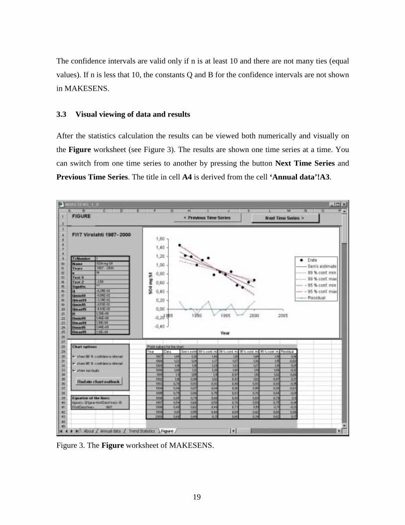
3.3 Visual viewing of data and results

After the statistics calculation the results can be viewed both numerically and visually on

the Figure worksheet (see Figure 3). The results are shown one time series at a time. You

can switch from one time series to another by pressing the button Next Time Series and

Previous Time Series. The title in cell A4 is derived from the cell ‘Annual data’!A3.

Figure 3. The Figure worksheet of MAKESENS.

20

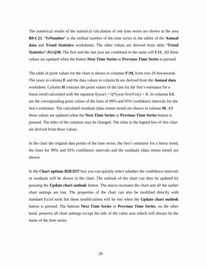
The numerical results of the statistical calculation of one time series are shown in the area

B9:C25. ‘TsNumber’ is the ordinal number of the time series in the tables of the Annual

data and Trend Statistics worksheets. The other values are derived from table ‘Trend

Statistics’!A5:Q30. The first and the last year are combined to the same cell C11. All these

values are updated when the button Next Time Series or Previous Time Series is pressed.

The table of point values for the chart is shown in columns F:M, from row 29 downwards.

The years in column F and the data values in column G are derived from the Annual data

worksheet. Column H contains the point values of the line for the Sen’s estimator for a

linear trend calculated with the equation f(year) = Q*(year-firstYear) + B. In columns I:L

are the corresponding point values of the lines of 99% and 95% confidence intervals for the

Sen’s estimator. The calculated residuals (data minus trend) are shown in column M. All

these values are updated when the Next Time Series or Previous Time Series button is

pressed. The titles of the columns may be changed. The titles in the legend box of this chart

are derived from these values.

In the chart the original data points of the time series, the Sen’s estimator for a linear trend,

the lines for 99% and 95% confidence intervals and the residuals (data minus trend) are

shown.

In the Chart options B28:D37 box you can quickly select whether the confidence intervals

or residuals will be shown in the chart. The outlook of the chart can then be updated by

pressing the Update chart outlook button. The macro recreates the chart and all the earlier

chart settings are lost. The properties of the chart can also be modified directly with

standard Excel tools but these modifications will be lost when the Update chart outlook

button is pressed. The buttons Next Time Series or Previous Time Series, on the other

hand, preserve all chart settings except the title of the value axis which will always be the

name of the time series.

21

4 Examples

The graphs produced with MAKESENS serve as a visual help for the interpretation of the

results given on the Trend Statistics worksheet. As an example the trend statistics of some

time series from the Finnish EMEP station Virolahti (FI17) are shown in Figures 4 – 6 and

briefly discussed here.

In Figure 4 there are two examples of annual time series: atmospheric SO42- concentration

and SO42- concentration in precipitation which nicely fulfill the premises of the statistical

methods used; The time series consist of annual averages with monotonously decreasing

trends. The residuals seem to be from a random distribution indicating that a linear model

may be applied. The statistical calculations give a high level of significance with narrow

angles between the confidence lines.

22

Figure 4. Annual time series and trend statistics of atmospheric SO42- concentrations (a) and

SO42- concentrations in precipitation (b) at Virolahti FI17.

The case of NH4+ concentration in precipitation is a bit more problematic (Figure 5). The

Mann-Kendall test indicates a decreasing trend at the 0.05 significance level but the Sen's

slope gives non-positive slope even at the 1% confidence interval. Thus the decreasing

trend seems to be more probable with the Sen's method than with the Mann-Kendall. The

reason to this difference may be that the presumptions of the Sen's method are not totally

Data Sen's estimate 99 % conf. min99 % conf. max 95 % conf. min 95 % conf. maxResidual

-0,2

0,0

0,2

0,4

0,6

0,8

1,0

1,2

1,4

1,6

1986 1988 1990 1992 1994 1996 1998 2000Year

mg S/l Name SO4 mg S/lYears 1987-2000N 14Test Z -3,50Signif icance ***Q -0,0625Qmin99 -0,0886Qmax99 -0,0339Qmin95 -0,0853Qmax95 -0,0443B 1,30Bmin99 1,46Bmax99 1,10Bmin95 1,44Bmax95 1,19

b

-0,5

0,0

0,5

1,0

1,5

2,0

1986 1988 1990 1992 1994 1996 1998 2000

Year

µg S/m3 Name SO4 µg S/m3Years 1987-2000N 14Test Z -4,05Signif icance ***Q -0,07Qmin99 -0,0975Qmax99 -0,036Qmin95 -0,0919Qmax95 -0,0462B 1,58Bmin99 1,72Bmax99 1,33Bmin95 1,68Bmax95 1,41

a

23

fulfilled. The Sen's method uses a linear model for the trend but here the slope seems to

diminish at the end which also can be seen from the residuals which are not random.

However the trend seems to be monotonic and thus the Mann-Kendall test is suitable. This

time series contains also two tied groups which may reduce the accuracy of these methods

with few data values as in this case.

Figure 5. Annual time series and trend statistics of NH4+ in precipitation at Virolahti FI17.

Data Sen's estimate 99 % conf. min99 % conf. max 95 % conf. min 95 % conf. maxResidual

-0,2

-0,1

0,0

0,1

0,2

0,3

0,4

0,5

0,6

0,7

0,8

1986 1988 1990 1992 1994 1996 1998 2000

Year

mg N/l Name NH4 mg N/lYears 1987-2000N 14Test Z -2,47Signif icance *Q -0,0175Qmin99 -0,0397Qmax99 0,00Qmin95 -0,0351Qmax95 -0,00379B 0,589Bmin99 0,735Bmax99 0,44Bmin95 0,728Bmax95 0,472

24

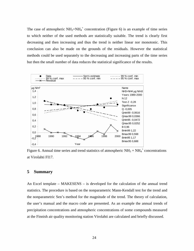
The case of atmospheric NH3+NH4+ concentration (Figure 6) is an example of time series

to which neither of the used methods are statistically suitable. The trend is clearly first

decreasing and then increasing and thus the trend is neither linear nor monotonic. This

conclusion can also be made on the grounds of the residuals. However the statistical

methods could be used separately to the decreasing and increasing parts of the time series

but then the small number of data reduces the statistical significance of the results.

Figure 6. Annual time series and trend statistics of atmospheric NH3 + NH4+ concentrations

at Virolahti FI17.

5 Summary

An Excel template – MAKESENS – is developed for the calculation of the annual trend

statistics. The procedure is based on the nonparametric Mann-Kendall test for the trend and

the nonparametric Sen’s method for the magnitude of the trend. The theory of calculation,

the user’s manual and the macro code are presented. As an example the annual trends of

precipitation concentrations and atmospheric concentrations of some compounds measured

at the Finnish air quality monitoring station Virolahti are calculated and briefly discussed.

Data Sen's estimate 99 % conf. min99 % conf. max 95 % conf. min 95 % conf. maxResidual

-0,4

-0,2

0,0

0,2

0,4

0,6

0,8

1,0

1,2

1,4

1988 1990 1992 1994 1996 1998 2000

Year

µg N/m3 NameNH3+NH4 µg N/m3Years 1989-2000N 12Test Z -0,28Signif icanceQ -0,005Qmin99 -0,0616Qmax99 0,0366Qmin95 -0,0472Qmax95 0,0252B 0,96Bmin99 1,22Bmax99 0,598Bmin95 1,17Bmax95 0,688

25

Examination of the time series is very important before performing and interpreting the

statistical calculations with MAKESENS. The Mann-Kendall method may be used in cases

where the possible trend can be assumed to be monotonic. In the Sen’s method it is

assumed that the trend is linear and the residuals are from the same distribution with zero

mean. The time series should fulfill these presumptions in order to produce correct

statistical results with MAKESENS.

In the Mann-Kendall test missing values are allowed and the data need not conform to any

particular distribution. The Sen’s method is not greatly affected by gross data errors or

outliers, and also it can be computed when data are missing.

AcknowledgementsThe authors thank the Nordic Council of Ministers for the financial support to this work.

6 References

Gilbert, R.O., 1987. Statistical methods for environmental pollution monitoring. Van

Nostrand Reinhold , New York.

Sirois, Allan, 1998. A Brief and Biased Overview of Time Series Analysis or How to Find

that Evasive Trend. In WMO report No. 133: WMO/EMEP workshop on Advanced

Statistical methods and their Application to Air Quality Data sets (Helsinki, 14-18

September 1998).

TFMM 2000. Minutes of the First Meeting of the Task Force (23 - 25 October 2000,

Vienna, Austria). http://www.ubavie.gv.at/tfmm/pages/meet.htm

26

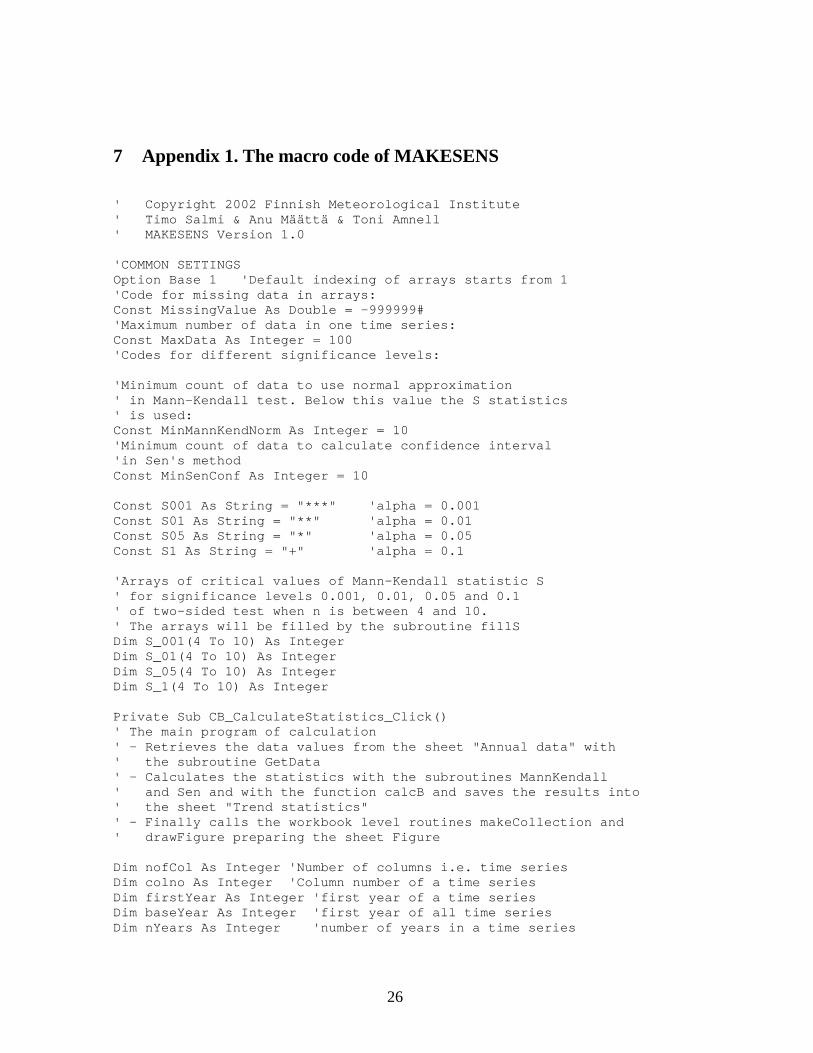
7 Appendix 1. The macro code of MAKESENS

' Copyright 2002 Finnish Meteorological Institute' Timo Salmi & Anu Määttä & Toni Amnell' MAKESENS Version 1.0

'COMMON SETTINGSOption Base 1 'Default indexing of arrays starts from 1'Code for missing data in arrays:Const MissingValue As Double = -999999#'Maximum number of data in one time series:Const MaxData As Integer = 100'Codes for different significance levels:

'Minimum count of data to use normal approximation' in Mann-Kendall test. Below this value the S statistics' is used:Const MinMannKendNorm As Integer = 10'Minimum count of data to calculate confidence interval'in Sen's methodConst MinSenConf As Integer = 10

Const S001 As String = "***" 'alpha = 0.001Const S01 As String = "**" 'alpha = 0.01Const S05 As String = "*" 'alpha = 0.05Const S1 As String = "+" 'alpha = 0.1

'Arrays of critical values of Mann-Kendall statistic S' for significance levels 0.001, 0.01, 0.05 and 0.1' of two-sided test when n is between 4 and 10.' The arrays will be filled by the subroutine fillSDim S_001(4 To 10) As IntegerDim S_01(4 To 10) As IntegerDim S_05(4 To 10) As IntegerDim S_1(4 To 10) As Integer

Private Sub CB_CalculateStatistics_Click()' The main program of calculation' - Retrieves the data values from the sheet "Annual data" with' the subroutine GetData' - Calculates the statistics with the subroutines MannKendall' and Sen and with the function calcB and saves the results into' the sheet "Trend statistics"' - Finally calls the workbook level routines makeCollection and' drawFigure preparing the sheet Figure

Dim nofCol As Integer 'Number of columns i.e. time seriesDim colno As Integer 'Column number of a time seriesDim firstYear As Integer 'first year of a time seriesDim baseYear As Integer 'first year of all time seriesDim nYears As Integer 'number of years in a time series

27

Dim n As Integer 'true data values in a time series'i.e. missing values are not considered

Dim x(MaxData) As Double 'Array for data values of a time seriesDim s As Integer 'Mann-Kendall test statistic for n=4..10Dim Z As Double 'Mann-Kendall test statistic for n>10Dim signif As String 'significance of trend'Sen's slope estimator Q and its 99% and 95% confidence levels:Dim Q As Double, Qmin99 As Double, Qmax99 As DoubleDim Qmin95 As Double, Qmax95 As Double'Constants B for equation of lines of Sen's slope and conf. intervals:Dim B As Double, Bmin99 As Double, Bmax99 As DoubleDim Bmin95 As Double, Bmax95 As Double

' The result cells are emptied before the calculation startsWorksheets("Trend Statistics").Range("E6:Q30") = ""

nofCol = Worksheets("Annual data").Cells(8, 2).valuebaseYear = Worksheets("Annual data").Cells(14, 1).valueCall fillS 'initializes arrays of Mann-Kendall probabilities

'Calculation of trend statistics for each time series at a timeFor colno = 2 To nofCol + 1

If Not GetData(colno, baseYear, firstYear, nYears, n, x) ThenExit Sub

End IfIf n >= 2 Then 'nothing can be computed, if n<2'First the existence of trend is tested using Mann-Kendall method.

Call MannKendall(nYears, x, s, Z, signif)If n < MinMannKendNorm Then

Worksheets("Trend Statistics").Cells(4 + colno, 5) = sElse

Worksheets("Trend Statistics").Cells(4 + colno, 6) = ZEnd IfWorksheets("Trend Statistics").Cells(4 + colno, 7) = signif

'Evaluation of Sen's slope estimator and confidence intervalsCall Sen(nYears, x, Q, Qmin99, Qmax99, Qmin95, Qmax95)Worksheets("Trend Statistics").Cells(4 + colno, 8) = QB = calcB(nYears, x, firstYear, baseYear, Q)Worksheets("Trend Statistics").Cells(4 + colno, 13) = B

If n >= MinSenConf ThenWorksheets("Trend Statistics").Cells(4 + colno, 9) = Qmin99Worksheets("Trend Statistics").Cells(4 + colno, 10) = Qmax99Worksheets("Trend Statistics").Cells(4 + colno, 11) = Qmin95Worksheets("Trend Statistics").Cells(4 + colno, 12) = Qmax95

'Coefficients B for equation of linear trend f(t)=Qt+BBmin99 = calcB(nYears, x, firstYear, baseYear, Qmin99)Bmax99 = calcB(nYears, x, firstYear, baseYear, Qmax99)Bmin95 = calcB(nYears, x, firstYear, baseYear, Qmin95)Bmax95 = calcB(nYears, x, firstYear, baseYear, Qmax95)Worksheets("Trend Statistics").Cells(4 + colno, 14) = Bmin99Worksheets("Trend Statistics").Cells(4 + colno, 15) = Bmax99Worksheets("Trend Statistics").Cells(4 + colno, 16) = Bmin95

28

Worksheets("Trend Statistics").Cells(4 + colno, 17) = Bmax95End If

End IfNext colno

' Draw the figure of the first componentSheets("Figure").Cells(9, 3).value = 1Sheets("Figure").Cells(10, 3).value = Sheets("Annual data").Cells(13,2).valueApplication.Run "makeCollection"Application.Run "DrawFigure"End Sub 'CB_CalculateStatistics_Click

Private Function GetData(ByVal colno As Integer, ByVal baseYear AsInteger, firstYear As Integer, nYears As Integer, n As Integer, x() AsDouble) As Boolean' Retrieving of data of one time series into the array x()' colno is the column of the worksheet "Annual data" where the' values of the time series exist.' The real number of annual values n in time series is calculated' If the cell is empty it is understood as a missing value.

Dim rowno As Integer 'row of the data cellDim lastYear As Integer 'last year of the time seriesDim nVal As Integer 'counter for number of true dataDim i As Integer 'counter for data loopDim Error As IntegerfirstYear = Worksheets("Annual data").Cells(10, colno).valuelastYear = Worksheets("Annual data").Cells(11, colno).valuenYears = lastYear - firstYear + 1

nVal = 0For i = 1 To nYears

If firstYear < baseYear ThenError = MsgBox("For the time series """ + _Worksheets("Annual data").Cells(13, colno).value + _""" first year is too early!")GetData = FalseExit Function

End Ifrowno = 13 + i + firstYear - baseYearIf IsEmpty(Worksheets("Annual data").Cells(rowno, colno)) Then

x(i) = MissingValueElse

nVal = nVal + 1x(i) = Worksheets("Annual data").Cells(rowno, colno)

End IfNext in = nValGetData = TrueEnd Function ' GetData

Private Sub MannKendall(ByVal nYears As Integer, x() As Double, s AsInteger, Z As Double, signif As String)

29

'Calculates the MannKendall test'Calls the function tiedSum'Uses the string constants S001, S01, S05 and S1

Dim absS As Integer 'value of absSDim varS As Double 'the variance of SDim absZ As Double 'value of abs(Z)Dim k As Integer, j As Integer 'counters for slopesDim n As Long 'number of true values in x()

Z = MissingValue ' returns MissingValue for Z' if they are not calculated

'Computing of the Mann-Kendall statistic S.signif = ""n = IIf(x(nYears) <> MissingValue, 1, 0)s = 0For k = 1 To nYears - 1

If x(k) <> MissingValue Thenn = n + 1For j = k + 1 To nYears

If x(j) <> MissingValue Thens = s + Sgn(x(j) - x(k))

End IfNext j

End IfNext k

If n < 4 Then'If n is less than 4, the method can not be used at all

Exit SubElseIf n < MinMannKendNorm Then'If n is between 4 and 10, S is compared directly to Mann-Kendallstatistics for S

absS = Abs(s)signif = Switch(absS >= S_001(n), S001, absS >= S_01(n), S01, absS >=

S_05(n), S05, absS >= S_1(n), S1, True, "")Else 'n>=MinMannKendNorm'If n is at least 10, the normal distribution is used'Firstly the variance VAR(S) is calculated'The correction term for ties is calculated by the function tiedSum

varS = (n * (n - 1) * (2 * n + 5) - tiedSum(nYears, x)) / 18#'Calculation of test statistic Z using S and its variance VAR(S)

Z = Switch(s > 0, (s - 1) / Sqr(varS), s < 0, (s + 1) / Sqr(varS), s= 0, 0#)'The absolute value of Z is compared to critical value Z[1-alpha/2]'which is obtained from the standard normal table. The presence and'significance of the trend is evaluated by testing four different'levels of significance: '0.001, 0.01, 0.05 and 0.1

absZ = Abs(Z)signif = Switch(absZ > 3.292, S001, absZ > 2.576, S01, absZ > 1.96,

S05, absZ > 1.645, S1, True, "")End If

End Sub 'MannKendall

30

Private Sub Sen(ByVal nYears As Integer, x() As Double, Q As Double,Qmin99 As Double, Qmax99 As Double, Qmin95 As Double, Qmax95 As Double)'Calculates Sen's slope estimator Q and its 99% (Qmax99,Qmin99)' and 95 % (Qmax95, Qmin95)confidence levels' Calls the function tiedSum and the subroutineCalulateConfidenceInterval

Dim nofQ As Integer 'number of value pairsDim Qarray(MaxData * (MaxData - 1) / 2) As Double 'Array for the slopesof value pairsDim k As Integer, j As Integer 'counters for loopsDim n As Long 'number of true values in x()Dim Calpha As Double 'C-alpha for calculation of conf.intervals of Q

'Computing of slopes of individual value pairs into QarraynofQ = 0 'used as counter for Qarrayn = IIf(x(nYears) = MissingValue, 0, 1)For k = 1 To nYears - 1

If x(k) <> MissingValue Thenn = n + 1For j = k + 1 To nYears

If x(j) <> MissingValue ThennofQ = nofQ + 1Qarray(nofQ) = (x(j) - x(k)) / (j - k)

End IfNext j

End IfNext k

'The median of individual slopes in Qarray is the Sen's'slope estimator. The median is calculated by the function "median".Q = median(nofQ, Qarray)

If n >= MinSenConf Then'The confidence intervals are calculated only if n is at least 10.'Computing of variance VAR(S) of Mann-Kendall statistics S.'The correction term for ties is calculated by the function tiedSum

varS = (n * (n - 1) * (2 * n + 5) - tiedSum(nYears, x)) / 18#

'The 100(1-alpha)% two-sided confidence intervals for the'Sen's slope are computed with two values of alpha: 0.01 and 0.05'which means 99% and 95% confidence intervals. The values of'Z[1-alpha/2] are obtained from the standard normal table.'Case alpha=0.01: Z[1-alpha/2]=Z[0.995]=2.576

Calpha = 2.576 * Sqr(varS)Call CalculateConfidenceInterval(Calpha, nofQ, Qarray, Qmin99,

Qmax99)

'Case alpha=0.05: Z[1-alpha/2]=1.96Calpha = 1.96 * Sqr(varS)Call CalculateConfidenceInterval(Calpha, nofQ, Qarray, Qmin95,

Qmax95)Else

31

Qmin99 = MissingValueQmax99 = MissingValueQmin95 = MissingValueQmax95 = MissingValue

End IfEnd Sub 'Sen

Private Function tiedSum(n As Integer, x() As Double) As Integer'Calculates sum related to tied groups(= two or more equal values)' for the variance of Mann-Kendall statistics S'n = number of values in the array x including missing values'Function tiedSum is called by subroutines Sen and MannKendallNorm

Dim m As Integer ' number of tied groupsDim tval() As Double ' data values of tied groupsReDim tval(n)Dim t() As Integer, nt As Integer ' number of data in tied groupsReDim t(n)Dim p, i As Integer 'indexes for the loopsDim newValue As BooleanDim tSum As Integer

'Calculation of the number of tied groups m and the number of data' in tied groups t()m = 0For i = 1 To n - 1

If x(i) <> MissingValue ThennewValue = TrueIf m > 0 Then

For p = 1 To mIf x(i) = tval(p) Then

newValue = False 'this value is alredy managedExit For

End IfNext p

End If

If newValue Thennt = 1 'number of equal values x(i)For p = i + 1 To n

If x(p) = x(i) Thennt = nt + 1

End IfNext p

If nt > 1 Then ' new group only if nt>1m = m + 1t(m) = nttval(m) = x(i)

End IfEnd If

End IfNext i

32

'Calculating the sum related to tied groups for variancetSum = 0If m > 0 Then

For p = 1 To mtSum = tSum + t(p) * (t(p) - 1) * (2 * t(p) + 5)

Next pEnd IftiedSum = tSumEnd Function 'tiedSum

Sub CalculateConfidenceInterval(ByVal Calpha As Double, ByVal nofQ AsInteger, Qarray() As Double, lowerLimit As Double, upperLimit As Double)'Computes confidence interval for Sen's slope estimate.'Input parameters: Calpha = Z[1-alpha/2],' nofQ - number of slopes of all data pairs' Qarray - array of slopes of all data pairs'Subroutine returns the lowerLimit and upperLimit.'Calls the subroutine SortArray'Is called by the subroutine Sen

Dim M1 As Double 'M1:th largest ordered slopeDim M2 As Double 'M2:th largest ordered slopeDim M1int As Integer 'integer part of M1 (>0)Dim M2int As Integer 'integer part of M2+1 (>0)Dim QarraySort() As DoubleReDim QarraySort(nofQ)

'The array Qarray is sorted to the array QarraySortCall SortArray(nofQ, Qarray, QarraySort)M1 = (nofQ - Calpha) / 2M2 = (nofQ + Calpha) / 2

If M1 > 1 Then'to be sure that index does not point outside QarraySort

M1int = Int(M1) 'find the integer part of M1'Interpolation of the lower limitlowerLimit = QarraySort(M1int) + (M1 - M1int) * (QarraySort(M1int

+ 1) - QarraySort(M1int))Else

lowerLimit = QarraySort(1)End If

If M2 < nofQ - 1 Then'to be sure that index does not point outside QarraySort

M2int = Int(M2 + 1) 'because the indexing of QarraySort beginsfrom zero

'Interpolation of the upper limitupperLimit = QarraySort(M2int) + (M2 + 1 - M2int) *

(QarraySort(M2int + 1) - QarraySort(M2int))Else

upperLimit = QarraySort(nofQ)End If

End Sub 'CalculateConfidenceInterval

33

Public Function calcB(nYears As Integer, x() As Double, firstYear AsInteger, baseYear As Integer, Q As Double) As Double' calculates the constant B for the equation of linear trend f(t)=Q*t+b.' The zero point of time axis is the "baseYear"' Calls the function medianDim n As Integer 'the number of true values in time seriesDim year As Integer 'the true year of the data valueDim i As Integer 'index for loopDim val() As Double 'array of differencesReDim val(nYears)

n = 0For i = 1 To nYears

year = firstYear + i - 1If x(i) <> MissingValue Then

n = n + 1val(n) = x(i) - Q * (year - baseYear)

End IfNext i

' the estimate for B is median of the calculated differencescalcB = median(n, val)End Function ' calcB

Private Function median(nofV As Integer, values() As Double) As Double' calculates median of values in the array values(), indexed from 1 tonofV' calls the subroutine sortArray' is called by the fuction calcB and by the subroutine Sen

Dim i As IntegerDim sortedValues() As DoubleReDim sortedValues(nofV)

Call SortArray(nofV, values, sortedValues)If nofV Mod 2 = 0 Then 'nofv is even

i = Int(nofV / 2)median = (sortedValues(i + 1) + sortedValues(i)) / 2

Else 'nOfvalues is oddmedian = sortedValues((nofV + 1) / 2)

End IfEnd Function 'median

Sub SortArray(ByVal nofV As Integer, values() As Double, sortedValues()As Double)'This subroutine ranks the values of an array from smallest to largest.'The sorting method is SELECTION SORT'The ranked values are stored into the other array called sortedValues.'Input parameters: nofV - number of values in the array values' values - values to be ranked, indexed from 1 to nofV'Subroutine returns the sorted array at sortedValues.'Is called by the function median and by the subroutine'CalculateConfidence interval

Dim ind As Integer, i As Integer, j As Integer

34

Dim minV As Double, maxV As DoubleDim carray() As Double 'the data is first copied to this arrayReDim carray(nofV)Dim ignoreV As Double 'value that is ignored in carray when sorting

For i = 1 To nofV 'Copy the original array to carraycarray(i) = values(i)

Next i

'Find the smallest and largest valueind = 1minV = carray(1) 'initialize the smallest valuemaxV = carray(1) 'initialize the largest valueFor i = 2 To nofV

If carray(i) < minV ThenminV = carray(i)ind = i

End IfIf carray(i) > maxV Then

maxV = carray(i)End If

Next i

sortedValues(1) = minV 'the smallest data valueignoreV = minV - 10 'smaller value than the smallest data valuecarray(ind) = ignoreV 'this value is later ignored in sorting

'now sort the valuesFor j = 2 To nofV

minV = maxVFor i = 1 To nofV

'find the minimum from the rest of the arrayIf carray(i) <= minV And carray(i) > ignoreV Then

minV = carray(i)ind = i

End IfNext isortedValues(j) = minVcarray(ind) = ignoreV 'from now on this element is ignored

Next jEnd Sub 'SortArray

Private Sub fillS()'Fills the arrays S_nnn of probabilities for two-tailed' Mann-Kendall test'The index of tables is the number of data if n=4...10'Each array entry is an absolute value of the Mann-Kendall' statistic S, with which the probability that there is no trend' is less than the probability level p related to the array:' S_001: p=0.001, S_01: p=0.01, S_05: p=0.05 and S_1: p=0.1.' Source of values: Gilbert, 1987, Table A18'Value 9999 indicates that the probability level can not be' reached with given number of data

35

Dim n As IntegerFor n = 4 To 10

S_001(n) = 9999S_01(n) = 9999S_05(n) = 9999S_1(n) = 9999

Next nS_001(7) = 21S_001(8) = 26S_001(9) = 30S_001(10) = 35S_01(6) = 15S_01(7) = 19S_01(8) = 22S_01(9) = 26S_01(10) = 29S_05(5) = 10S_05(6) = 11S_05(7) = 15S_05(8) = 18S_05(9) = 20S_05(10) = 23S_1(4) = 6S_1(5) = 8S_1(6) = 11S_1(7) = 13S_1(8) = 16S_1(9) = 18S_1(10) = 21

End Sub