Makara Journal of Technology Makara Journal of Technology

Volume 23 Number 2 Article 6

8-2-2019

3D FDTD Method for Modeling of Seismo-Electromagnetics 3D FDTD Method for Modeling of Seismo-Electromagnetics

Disturbance on Crustal Earth Disturbance on Crustal Earth

Nabila Husna Shabrina Faculty of Engineering and Informatics, Universitas Multimedia Nusantara, Tangerang 15811, Indonesia

Yasuhide Hobara Department of Communication Engineering and Informatics, Graduate School of Informatics and Engineering, The University of Electro–Communications, Chofu, Tokyo 182-8585, Japan

Achmad Munir Radio Telecommunication and Microwave Laboratory, School of Electrical Engineering and Informatics, Institut Teknologi Bandung, Bandung 40132, Indonesia, munir@ieee.org

Follow this and additional works at: https://scholarhub.ui.ac.id/mjt

Part of the Chemical Engineering Commons, Civil Engineering Commons, Computer Engineering

Commons, Electrical and Electronics Commons, Metallurgy Commons, Ocean Engineering Commons, and

the Structural Engineering Commons

Recommended Citation Recommended Citation Shabrina, Nabila Husna; Hobara, Yasuhide; and Munir, Achmad (2019) "3D FDTD Method for Modeling of Seismo-Electromagnetics Disturbance on Crustal Earth," Makara Journal of Technology: Vol. 23 : No. 2 , Article 6. DOI: 10.7454/mst.v23i2.3715 Available at: https://scholarhub.ui.ac.id/mjt/vol23/iss2/6

This Article is brought to you for free and open access by the Universitas Indonesia at UI Scholars Hub. It has been accepted for inclusion in Makara Journal of Technology by an authorized editor of UI Scholars Hub.

Makara J. Technol. 23/2 (2019), 84-91 doi: 10.7454/mst.v23i2.3715

August 2019 | Vol. 23 | No. 2 84

3D FDTD Method for Modeling of Seismo-Electromagnetics Disturbance on Crustal Earth

Nabila Husna Shabrina1, Yasuhide Hobara2, and Achmad Munir3*

1. Faculty of Engineering and Informatics, Universitas Multimedia Nusantara, Tangerang 15811, Indonesia 2. Department of Communication Engineering and Informatics, Graduate School of Informatics and Engineering,

The University of Electro–Communications, Chofu, Tokyo 182-8585, Japan 3. Radio Telecommunication and Microwave Laboratory, School of Electrical Engineering and Informatics,

Institut Teknologi Bandung, Bandung 40132, Indonesia

*e-mail: munir@ieee.org

Abstract

The paper deals with the modelling of seismo-electromagnetics disturbance on the crustal earth by use of three-dimensional (3D) finite-difference time-domain (FDTD) method. The model is built up by discretizing the frontier geographical region between Java Island and Sumatra Island in a cylindrical coordinate system-based 3D object. The proposed method is applied to compute and analyze electromagnetics (EM) fields of the observed very low frequency (VLF) wave used for the investigation. Boundary condition of uniaxial perfectly matched layer (UPML) are applied surrounding the area of computation for truncating the object of simulation. The investigation are focused on the propagation time of observed VLF wave and its amplitude variation between the observation point and disturbance pulse. The result shows that the propagation time is significantly affected by the distance of observation point and the permittivity of propagation medium. Meanwhile, the addition pulse associated with the earthquake influences the amplitude of observed VLF wave instead of its frequency.

Abstrak

Metode FDTD 3D untuk Pemodelan Gangguan Seismo-elektromagnetik pada Kerak Bumi. Penelitian ini bertujuan untuk memodelkan fenomena seismo-electromagnetics dengan metode finite-difference time-domain (FDTD) tiga dimensi (3D). Pemodelan dibangun dengan mendiskretisasi peta geografis pada perbatasan antara Pulau Jawa dan Pulau Sumatra dalam bentuk 3D berbasis koordinat silinder. Metode yang diusulkan digunakan untuk menghitung dan menganalisis medan elektromagnetik (EM) pada pengamatan gelombang frekuensi Very Low Frequency (VLF) yang digunakan dalam investigasi. Kondisi batas Uniaxial Perfectly Matched Layer (UPML) digunakan pada sekeliling area komputasi untuk membatasi objek simulasi. Investigasi difokuskan pada pengamatan waktu propagasi dan variasi amplitudo gelombang antara titik pengamatan dan sumber gangguan. Hasil penelitian menunjukkan bahwa waktu propagasi sangat dipengaruhi oleh jarak titik pengamatan dan permitivitas dari medium propagasi. Adapun penambahan gelombang pulsa yang diasosiasikan sebagai gempa bumi berpengaruh hanya terhadap amplitudo gelombang VLF yang diamati dan bukan terhadap frekuensinya. Keywords: 3D FDTD method, seismo-electromagnetics, UPML, VLF wave 1. Introduction During 2018 there were 382 Earth Quakes (EQs) with magnitude greater than or equal to 5 scale of Righter (SR) happened in Indonesia [1]. The two most recent dreadful EQs happened in Lombok, August 2018 causing around 500 people died and in Palu, October 2018 which was also followed by tsunami and killed

around 2000 people [2] [3]. Those situations make Indonesia as a country with high EQs potentials. Therefore, EQs prediction is required as an early mitigation. Formerly, EQs prediction could only be determined by seismic activities. However, in the past decades, research shows that the EM phenomena could also be used as EQs precursors [4] [7].

FDTD Modeling for Seismo-Electromagnetics Disturbance

Makara J. Technol.  1  August 2019 Vol. 23 No. 2 

85

The EM phenomena associated with EQs is commonly known as seismo-electromagnetics. An observation in [8] shows that when strong EQs happened, both satellite and ground observation detected wide-frequency band of EM waves. Some satellites e.g. GEOS-2, DE2, Intercosmos-19 and 24, indicated several cases of EM perturbations correlated with EQs have also been reported [9]. Moreover, in a mission to observe seismo-electromagnetics phenomena, China has launched China Seismo-Electromagnetic Satellite (CSES) on February 2018 [10]. Seismo-electromagnetic phenomena is usually observed in Very Low Frequency (VLF) wave. The transient and anomaly of VLF wave in ionosphere were found as an indication to EQs. A number of researches have been done to observe the correlation of VLF wave in ionospheric layer which occurred as an effect of seismic activities which lead to EQs [11], 12]. To have better comprehension especially in seismo-electromagnetics phenomena, understanding of EM waves and its phenomena is absolutely necessary. It is well-known that EM waves could be computed and analyzed conveniently using numerical computation. In last decades, the use of numerical computation methods for analyzing EM waves has grown up rapidly. There were several numerical methods frequently applied to analyze EM waves including Finite Difference Time Domain (FDTD), Finite Volume Method (FVM), Finite Element Method (FEM), and Method of Moment (MoM). Each of methods has own merits as well as demerits. Here, FDTD method is implemented as it has several superiorities in terms of time efficiency, memory saving, straightforward understanding, and its robustness to solve electromagnetic problems [13]. Recently, the use FDTD method especially in three dimensional (3D) based on cylindrical coordinate system has been implemented to study and model the crustal earth [14]–[16]. An observation of seismo-electromagnetics phenomena using 2D FDTD method has also been reported [17]. To advance the previous research in [17],[18], this paper deals with the modelling of seismo-electromagnetics disturbance on crustal earth using 3D FDTD based on cylindrical coordinate system. The propagation time between the observation point and disturbance is investigated intensively. Meanwhile the amplitude variation of observed VLF wave as an effect of additional pulse associated with EQs is also analyzed. 2. Methods and Modelling

    (1)

    (2)

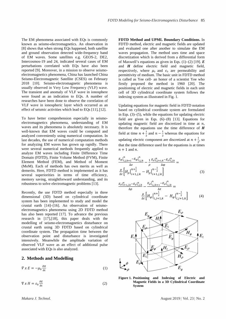
FDTD Method and UPML Boundary Conditions. In FDTD method, electric and magnetic fields are updated and evaluated one after another to simulate the EM waves propagation. The method uses time and space discretization which is derived from a differential form of Maxwell’s equations as given in Eqs. (1)(2) [19]. E and H define electric field and magnetic field, respectively, where 0 and 0 are permeability and permittivity of medium. The basic unit in FDTD method is called as Yee cell- an honor of a scientist Yee who firstly proposed the method in 1960 [20]. The positioning of electric and magnetic fields in each unit cell of 3D cylindrical coordinate system follows the indexing system as illustrated in Fig. 1. Updating equations for magnetic field in FDTD notation based on cylindrical coordinate system are formulated in Eqs. (3)(5), while the equations for updating electric field are given in Eqs. (6)(8) [13]. Equations for updating magnetic field are discretized in time at , therefore the equations use the time difference of

field at time and whereas the equations for

updating electric component are discretized at , so

that the time difference used for the equations is at times 1 and .

, , , ,

∆

| , , | , ,

∆

 ∆ , , , ,

(3)

| , , | , ,

∆

, , , ,

∆

                         ∆ , ,

 , ,

(4)

Figure 1. Positioning and Indexing of Electric and Magnetic Fields in a 3D Cylindrical Coordinate System

Shabrina, et al.

Makara J. Technol. 1 August 2019 | Vol. 23 | No. 2

86

, , , ,

∆

, , , ,

∆

                          ∆

|, ,

  |, ,

(5)

|, ,

|, ,

∆

, , , ,

∆

                           ∆ , ,

 , ,

(6)

, , , ,

∆

|, ,

|, ,

∆

                          ∆ , ,

 , ,

(7)

, , , ,

∆

, , , ,

∆

                           ∆

| , ,   | , , (8)

Basically, FDTD method uses Perfect Electric Conductor (PEC) as a boundary condition. In PEC, electric and magnetic fields reflect the simulation area as it reaches the outer region. It is occurred because the electric field in the outer region of PEC is defined as zero. This characteristic leads the interference between source wave and reflected wave. Therefore, there is another method of boundary condition to overcome the interference issue called as Perfectly Matched Layer (PML) developed in 1994 by Jean-Pierre Berenger [21]. PML boundary conditions use absorbing layer to absorb EM waves without reflection [21]. Some PML boundary conditions frequently applied are Convolutional Perfectly Matched Layer (CPML), Uniaxial Perfectly Matched Layer (UPML), and Split-Field PML. In this work, UPML is implemented as a boundary condition due to its convenient. Moreover, UPML is the most efficient to implement because its time domain equation is symmetric hyperbolic and has the smallest amount of equations [22]. UPML applies anisotropic tensor for permittivity and permeability with the Maxwell formula as shown in Eqs. (9) (10) where   denotes a diagonal tensor in 3D cylindrical coordinate system.              (9)

             (10) Implementation of electric and magnetic fields in UPML is based on the correlation between electric flux

and magnetic flux in which these are also related to and , respectively. The formulas for calculating  ,   , and   in FDTD notation are expressed in

Eqs. (11)-(14). 0 and 0 are permeability and

permittivity of medium, respectively, where is constant and is lossy medium conductivity which its value depends on the axis.  

, ,

 

2 ∅   ∅∆

2 ∅   ∅∆ 

, ,

2 ∆

2 ∅   ∅∆

, ,

/

, ,

/ 

∆∅

                      , ,

/

, ,

/ 

∆                         11

 , ,

2 ∅   ∅∆

2 ∅   ∅∆ 

, ,

 2 ∆

2 ∅   ∅∆

, , , , 

∆∅

∅ , , ∅ , , 

∆                                                12

, ,

 2   ∆

2   ∆  

, ,

 1 2   ∆

2   ∆   

, ,

 

  1 2   ∆

2   ∆   

, ,

                                     13

, , /

/

 2   ∆

2   ∆  

, ,

 1 2   ∆

2   ∆   

, ,

  1 2   ∆

2   ∆   

, ,                              14

Modelling Seismo-electromagnetic Disturbance on Crustal Earth. To model seismo-electromagnetic disturbance, FDTD method in 3D cylindrical coordinate system is employed. The -axis is used to model the depth of earth, the -axis is associated with the width of earth, and the -axis represents the length of earth. The object of simulation is a frontier geographical region between Sumatra Island and Java Island with the dimension of 40 km x 200 km x 220 km. The

FDTD Modeling for Seismo-Electromagnetics Disturbance

Makara J. Technol.  1  August 2019 Vol. 23 No. 2 

87

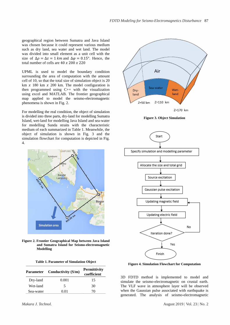
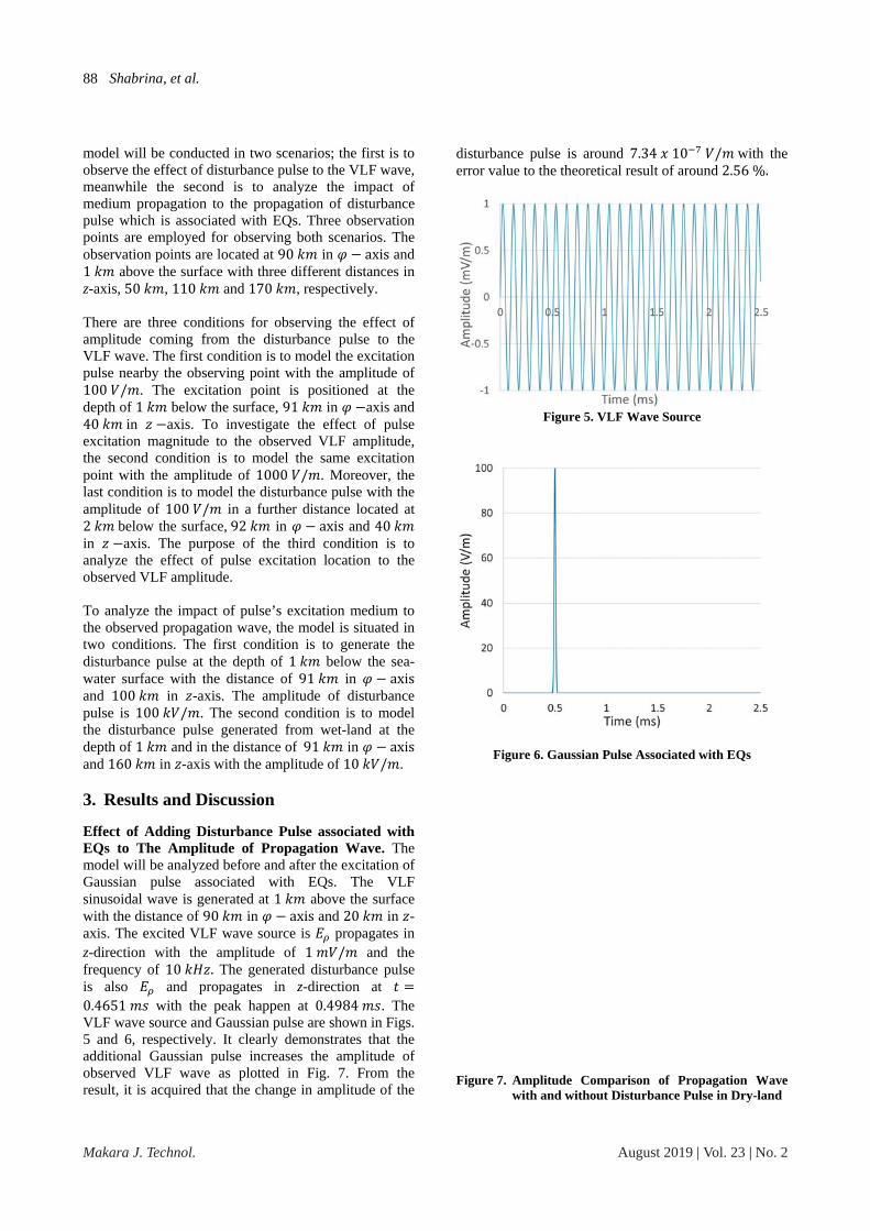
geographical region between Sumatra and Java Island was chosen because it could represent various medium such as dry land, sea water and wet land. The model was divided into small element as a unit cell with the size of ∆ ∆ 1   and ∆ 0.15°. Hence, the total number of cells are 40   200   220 UPML is used to model the boundary condition surrounding the area of computation with the amount cell of 10, so that the total size of simulation object is 20 km 180 km 200 km. The model configuration is then programmed using C++ with the visualization using excel and MATLAB. The frontier geographical map applied to model the seismo-electromagnetic phenomena is shown in Fig. 2. For modelling the real condition, the object of simulation is divided into three parts, dry-land for modelling Sumatra Island, wet-land for modelling Java Island and sea-water for modelling Sunda straits with the characteristic medium of each summarized in Table 1. Meanwhile, the object of simulation is shown in Fig. 3 and the simulation flowchart for computation is depicted in Fig. 4.

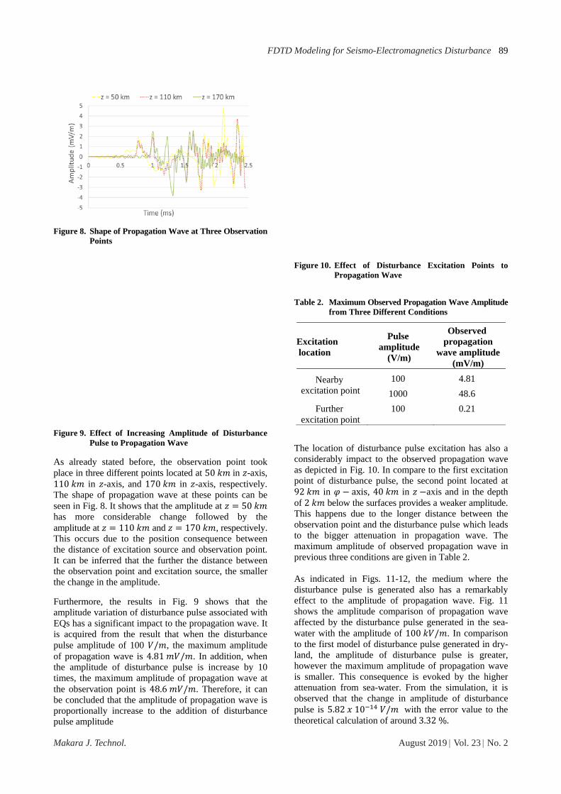
Figure 2. Frontier Geographical Map between Java Island

and Sumatra Island for Seismo-electromagnetic Modelling

Table 1. Parameter of Simulation Object

Parameter Conductivity (S/m) Permittivity coefficient

Dry-land 0.001 15

Wet-land 5 30

Sea-water 0.01 70

Figure 3. Object Simulation

Figure 4. Simulation Flowchart for Computation

3D FDTD method is implemented to model and simulate the seismo-electromagnetic on crustal earth. The VLF wave in atmosphere layer will be observed when the Gaussian pulse associated with earthquake is generated. The analysis of seismo-electromagnetic

Shabrina, et al.

Makara J. Technol. 1 August 2019 | Vol. 23 | No. 2

88

model will be conducted in two scenarios; the first is to observe the effect of disturbance pulse to the VLF wave, meanwhile the second is to analyze the impact of medium propagation to the propagation of disturbance pulse which is associated with EQs. Three observation points are employed for observing both scenarios. The observation points are located at 90  in axis and 1  above the surface with three different distances in z-axis, 50  , 110  and 170  , respectively. There are three conditions for observing the effect of amplitude coming from the disturbance pulse to the VLF wave. The first condition is to model the excitation pulse nearby the observing point with the amplitude of 100  / . The excitation point is positioned at the depth of 1  below the surface, 91  in axis and 40   in axis. To investigate the effect of pulse excitation magnitude to the observed VLF amplitude, the second condition is to model the same excitation point with the amplitude of 1000  / . Moreover, the last condition is to model the disturbance pulse with the amplitude of 100  / in a further distance located at 2   below the surface, 92  in axis and 40  in axis. The purpose of the third condition is to analyze the effect of pulse excitation location to the observed VLF amplitude. To analyze the impact of pulse’s excitation medium to the observed propagation wave, the model is situated in two conditions. The first condition is to generate the disturbance pulse at the depth of 1  below the sea-water surface with the distance of 91  in axis and 100  in -axis. The amplitude of disturbance pulse is 100  / . The second condition is to model the disturbance pulse generated from wet-land at the depth of 1  and in the distance of  91  in axis and 160  in -axis with the amplitude of 10  / . 3. Results and Discussion

Effect of Adding Disturbance Pulse associated with EQs to The Amplitude of Propagation Wave. The model will be analyzed before and after the excitation of Gaussian pulse associated with EQs. The VLF sinusoidal wave is generated at 1  above the surface with the distance of 90  in axis and 20  in -axis. The excited VLF wave source is propagates in z-direction with the amplitude of 1  / and the frequency of 10  . The generated disturbance pulse is also and propagates in z-direction at 0.4651  with the peak happen at 0.4984  . The VLF wave source and Gaussian pulse are shown in Figs. 5 and 6, respectively. It clearly demonstrates that the additional Gaussian pulse increases the amplitude of observed VLF wave as plotted in Fig. 7. From the result, it is acquired that the change in amplitude of the

disturbance pulse is around 7.34   10   /  with the error value to the theoretical result of around 2.56 %.

Figure 5. VLF Wave Source

Figure 6. Gaussian Pulse Associated with EQs

Figure 7. Amplitude Comparison of Propagation Wave

with and without Disturbance Pulse in Dry-land

FDTD Modeling for Seismo-Electromagnetics Disturbance

Makara J. Technol.  1  August 2019 Vol. 23 No. 2 

89

Figure 8. Shape of Propagation Wave at Three Observation Points

Figure 9. Effect of Increasing Amplitude of Disturbance Pulse to Propagation Wave

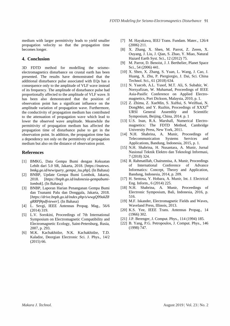
As already stated before, the observation point took place in three different points located at 50   in -axis, 110  in -axis, and 170  in -axis, respectively. The shape of propagation wave at these points can be seen in Fig. 8. It shows that the amplitude at 50  has more considerable change followed by the amplitude at 110  and 170  , respectively. This occurs due to the position consequence between the distance of excitation source and observation point. It can be inferred that the further the distance between the observation point and excitation source, the smaller the change in the amplitude.

Furthermore, the results in Fig. 9 shows that the amplitude variation of disturbance pulse associated with EQs has a significant impact to the propagation wave. It is acquired from the result that when the disturbance pulse amplitude of 100 / , the maximum amplitude of propagation wave is 4.81  / . In addition, when the amplitude of disturbance pulse is increase by 10 times, the maximum amplitude of propagation wave at the observation point is 48.6  / . Therefore, it can be concluded that the amplitude of propagation wave is proportionally increase to the addition of disturbance pulse amplitude

Figure 10. Effect of Disturbance Excitation Points to Propagation Wave

Table 2. Maximum Observed Propagation Wave Amplitude

from Three Different Conditions

Excitation location

Pulse amplitude

(V/m)

Observed propagation

wave amplitude (mV/m)

Nearby excitation point

100 4.81

1000 48.6

Further excitation point

100 0.21

The location of disturbance pulse excitation has also a considerably impact to the observed propagation wave as depicted in Fig. 10. In compare to the first excitation point of disturbance pulse, the second point located at 92  in axis, 40  in axis and in the depth of 2  below the surfaces provides a weaker amplitude. This happens due to the longer distance between the observation point and the disturbance pulse which leads to the bigger attenuation in propagation wave. The maximum amplitude of observed propagation wave in previous three conditions are given in Table 2. As indicated in Figs. 11-12, the medium where the disturbance pulse is generated also has a remarkably effect to the amplitude of propagation wave. Fig. 11 shows the amplitude comparison of propagation wave affected by the disturbance pulse generated in the sea-water with the amplitude of 100  / . In comparison to the first model of disturbance pulse generated in dry-land, the amplitude of disturbance pulse is greater, however the maximum amplitude of propagation wave is smaller. This consequence is evoked by the higher attenuation from sea-water. From the simulation, it is observed that the change in amplitude of disturbance pulse is 5.82   10   /   with the error value to the theoretical calculation of around 3.32 %.

Shabrina, et al.

Makara J. Technol. 1 August 2019 | Vol. 23 | No. 2

90

Figure 11. Amplitude Comparison of Propagation Wave with and without Disturbance Pulse in Sea-water

Figure 12. Amplitude Comparison of Propagation Wave with and without Disturbance Pulse in Wet-land

Meanwhile as plotted in Fig. 12, the disturbance pulse generated in wet-land with the amplitude of 10  / has also an impact to the propagation wave. In this model, the disturbance pulse is generated 100 times higher than the amplitude of disturbance pulse in dry-land. Yet, the change in amplitude of observed propagation wave only 10 times higher than the result as depicted in Fig. 7. This happens due to the conductivity characteristic of wet-land which is higher than the conductivity of dry-land. The change in amplitude of disturbance pulse is 3.04   10   /  with the error value to the theoretical approach of around 0.18 %. Summary for the change in amplitude of disturbance pulse in three mediums is given in Table 3. Effect of Adding Disturbance Pulse associated with EQs to The Frequency of Propagation Wave. As shown in Fig. 13, the frequency of observed VLF wave is unaffected by the excitation of disturbance pulse which is associated with EQs. This happens due to the absence of frequency component in the disturbance pulse that can influence the frequency of propagation wave

Table 3. Change in Amplitude of Disturbance Pulse in Three Mediums

Medium excitation

The change in amplitude of disturbance pulse (V)

Error (%)

Dry-land 7.34   10 2.56

Wet-land 3.04   10 0.18 Sea-water 5.82   10   3.32

Figure 13. Effect of Disturbance Pulse to Frequency of

Propagation Wave

Table 4. Propagation Time of Disturbance Pulse

Medium observation

Theoretical time (ms)

Simulation time (ms)

Error (%)

Dry-land 0.5727 0.5726 0.0025

Wet-land 0.6000 0.6005 0.008

Sea-water 0.6494 0.6490 0.0062 Propagation Time of Disturbance Pulse Associated with EQs. Based on the simulation results as given in Table 4, it shows that the propagation time required by the disturbance pulse from the excitation point in dry-land to arrive at the observation point located at 90  in axis, 1  above the surfaces and 50  in -axis is 0.5726  , while the theoretical result is 0.5727  , so that the error value is around 0.0025%. Furthermore, the theoretical calculation and simulation result of propagation time observed at 50  in -axis is 0.6494  and 0.6490  , respectively. The error value obtained in this observation point is around 0.0062%. The last observation point which is located at

170  has simulated propagation time of 0.6005  , while the theoretical approach has 0.6000  . Hence, the error value from the last observation point is around 0.008%.  These results are satisfying theoretical prediction where the propagation

FDTD Modeling for Seismo-Electromagnetics Disturbance

Makara J. Technol.  1  August 2019 Vol. 23 No. 2 

91

medium with larger permittivity leads to yield smaller propagation velocity so that the propagation time becomes longer. 4. Conclusion 3D FDTD method for modelling the seismo-electromagnetics disturbance on crustal earth has been presented. The results have demonstrated that the additional disturbance pulse associated with EQs has a consequence only to the amplitude of VLF wave instead of its frequency. The amplitude of disturbance pulse had proportionally affected to the amplitude of VLF wave. It has been also demonstrated that the position of observation point has a significant influence on the amplitude variation of propagation wave. Furthermore, the conductivity of propagation medium has contributed to the attenuation of propagation wave which lead to lower the observed wave amplitude. Meanwhile the permittivity of propagation medium has affected the propagation time of disturbance pulse to get in the observation point. In addition, the propagation time has a dependency not only on the permittivity of propagation medium but also on the distance of observation point.

References [1] BMKG, Data Gempa Bumi dengan Kekuatan

Lebih dari 5.0 SR, Jakarta, 2018. [https://inatews. bmkg.go.id/new/query_gempa_isu.php]. (In Bahasa)

[2] BNBP, Update Gempa Bumi Lombok, Jakarta, 2018. [https://bnpb.go.id/indonesia-gempabumi-lombok]. (In Bahasa)

[3] BNBP, Laporan Harian Penanganan Gempa Bumi dan Tsunami Palu dan Donggala, Jakarta, 2018. [https://drive.bnpb.go.id/index.php/s/wwgQ99akZ8gRRPf#pdfviewer]. (In Bahasa)

[4] L. Sevgi, IEEE Antennas Propag. Mag., 56/6 (2014) 319.

[5] L.V. Sorokini, Proceedings of 7th International Symposium on Electromagnetic Compatibility and Electromagnetic Ecology, Saint-Petersburg, Rusia, 2007, p. 293.

[6] M.K. Kachakhidze, N.K. Kachakhidze, T.D. Kaladze, Deorgian Electronic Sci. J. Phys., 14/2 (2015) 66.

[7] M. Hayakawa, IEEJ Trans. Fundam. Mater., 126/4 (2006) 211.

[8] X. Zhang, X. Shen, M. Parrot, Z. Zeren, X. Ouyang, J. Liu, J. Qian, S. Zhao, Y. Miao, Natural Hazard Earth Syst. Sci., 12 (2012) 75.

[9] M. Parrot, D. Benoist, J. J. Berthelier, Planet Space Sci., 54 (2006) 441.

[10] X. Shen, X. Zhang, S. Yuan, L. Wang, J. Cao, J. Huang, X. Zhu, P. Piergiorgio, J. Dai, Sci. China Technol. Sci., 61 (2018) 634.

[11] N. Yaacob, A.L. Yusof, M.T. Ali, S. Subahir, W. Norsyafizan, W. Muhamad, Proceedings of IEEE Asia-Pasific Conference on Applied Electro-magnetics, Port Dickson, Malaysia, 2010, p. 1.

[12] Z. Zhima, Z. XueMin, S. XuHui, S. WeiHuai, N. DongMei, and Y. Ruzhin, Proceedings of XXXIth URSI General Assembly and Scientific Symposium, Beijing, China, 2014. p. 1

[13] U.S. Inan, R.A. Marshall, Numerical Electro-magnetics: The FDTD Method, Cambridge University Press, New York, 2011.

[14] N.H. Shabrina, A. Munir, Proceedings of Telecommunication Systems Services and Applications, Bandung, Indonesia, 2015, p. 1.

[15] N.H. Shabrina, H. Nusantara, A. Munir, Jurnal Nasional Teknik Elektro dan Teknologi Informasi, 7 (2018) 324.

[16] R. Rahmatillah, Chairunnisa, A. Munir, Proceedings of International Conference of Advance Informatics: Concept, Theory and Application, Bandung, Indonesia, 2014, p. 209.

[17] H. Sentosa, Y. Hobara, A. Munir, Int. J. Electrical Eng. Inform., 6 (2014) 225.

[18] N.H. Shabrina, A. Munir, Proceedings of Electronic Symposium, Bali, Indonesia, 2016, p. 516.

[19] M.F. Iskander, Electromagnetic Fields and Waves, Waveland Press, Illinois, 2013.

[20] K.S. Yee, IEEE Trans. Antennas Propag., 14 (1966) 302.

[21] J.P. Berenger, J. Comput. Phys., 114 (1994) 185. [22] B. Yang, P.G. Petropoulos, J. Comput. Phys., 146

(1998) 747.