Mainz-02-11-041

Colloidal Sedimentation

Ard LouisDept. of Chemistry

Movie from Paddy Royall (Utrecht); Polystyrene

The interplay of Brownian & Hydrodynamic Forces

Mainz-02-11-042

Sedimentation of colloids

gFkT

F

F

2

6sed

mgV R

R

The bigger the particles the faster they sediment

sedF V mg

6 ( )R Stokes

buoyant mass

Mainz-02-11-043

George Gabriel Stokes (1851)

sed

mgv

Albert Einstein (1905)

kTD

advection

diffusionsed

B

RvPe

D

mgRk T

Peclet

Robert Brown (1827)

Brownian motion

Mainz-02-11-044

Pe=10

Brownian Dynamics

240 discs in a closed

container

Sedimentation

Mainz-02-11-045

G.K. Batchelor, J. Fluid Mech. 52, 245 (1972)

! 0 0.15sedBig effect v for

Hydrodynamic forcesare long-ranged

1( )

8ˆˆv r F

rI rr

3

0 (1 6.55 )sed sedv v

1

r

Mainz-02-11-046Pe=10

Hydrodynamics?

240 discs in a closed container

+ 200,000 small fluid particles to generate Brownian and hydrodynamic forces

Hydrodynamics induces correlated velocity fluctuations

Sedimentation

Mainz-02-11-047

Hydrodynamic fluctuations?

Segre et al. PRL 79,2574 (1997)

Caflish & Luke, Phys. Fluids 28, 259 (1985)

22

2 2

1

ii

N

ii

fv

L

v v L

Uncorrelated concentration fluctuations induce velocity fluctuations

Mainz-02-11-048

Hydrodynamic Screening?

Segre et al. PRL 79,2574 (1997)

Still a mystery!

•Walls on sides?

•Wall at bottom?

•Stratification?

•Noise induced phase transitions?

Mainz-02-11-049

What about Mr Brown?

Brownian and Hydrodynamic fluctuations?

Thermal v.s. non-thermal noise?

Mainz-02-11-0410

The problem

Colloids >> solvent molecules Stupendous amount of solvent molecules;

E.g 1011 water molecules per R=1 micron colloid.

Coarse-graining is necessary

Colloid Solvent molecule

Mainz-02-11-0411

Computational methods Stokesian Dynamics (SD) Dissipative Particle Dynamics (DPD) Lattice Boltzmann (LB) Stochastic Rotation Dynamics (SRD)

Mainz-02-11-0412

Stokesian Dynamics Approximate solution of Stokes’

equation for many spheresin a solvent (“Oseen tensor”)

No explicit solvent Only correct at low densities of spheres Only correct in the bulk Non-spherical particles extremely difficult Relatively expensive

J.F. Brady and G. Bossis, Ann. Rev. Fluid Mech. 20, 111 (1988)

Mainz-02-11-0413

Dissipative Particle Dynamics

Each DPD particle representsa group of solvent molecules

Pairwise conservative forces Pairwise friction & random forces

Conservation of momentum(unlike traditional Brownian Dynamics)

R.D. Groot and P.B. Warren, J. Chem. Phys. 107, 4423 (1997)See also Sodderman, Dünweg and Kremer, PRE 69, 046702 (2003)

Mainz-02-11-0414

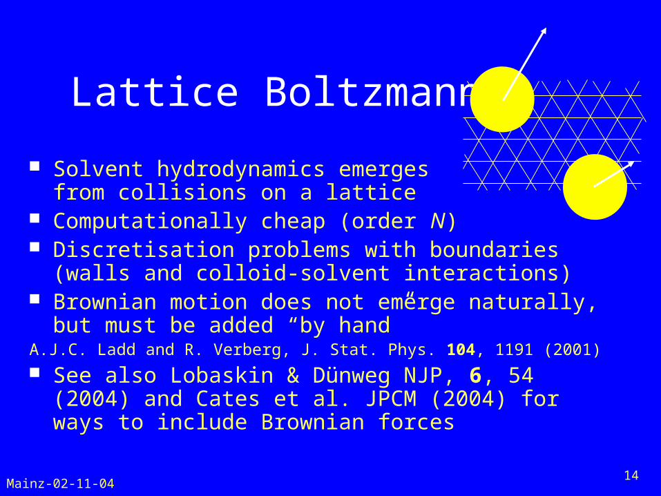
Lattice Boltzmann

Solvent hydrodynamics emergesfrom collisions on a lattice

Computationally cheap (order N) Discretisation problems with boundaries (walls

and colloid-solvent interactions) Brownian motion does not emerge naturally, but

must be added “by hand”A.J.C. Ladd and R. Verberg, J. Stat. Phys. 104, 1191 (2001)

See also Lobaskin & Dünweg NJP, 6, 54 (2004) and Cates et al. JPCM (2004) for ways to include Brownian forces

Stochastic Rotation Dynamics

a.k.a.Multi-Particle Collision Dynamics

a.k.a.Malevanets-Kapral Method

Mainz-02-11-0416

Stochastic Rotation Dynamics

Solvent hydrodynamics emergesfrom collisions in coarse-grainedcells

Computationally cheap (order N) Particles move in continuous space,

so no discretisation problems Brownian motion emerges naturally

A. Malevanets and R. Kapral, J. Chem. Phys. 110, 8605 (1999)T. Ihle and D.M. Kroll, Phys. Rev. E 67, 066705 (2003); ibid. 066706 (2003)

Mainz-02-11-0417

How does it work? Represent the solvent by N point-like

particles (SRD particles) In between collisions, the SRD particles do

not interact with each other (ideal gas)

Mainz-02-11-0418

How does it work? Streaming step:

2

2i

i

d rm Fdt

Mainz-02-11-0419

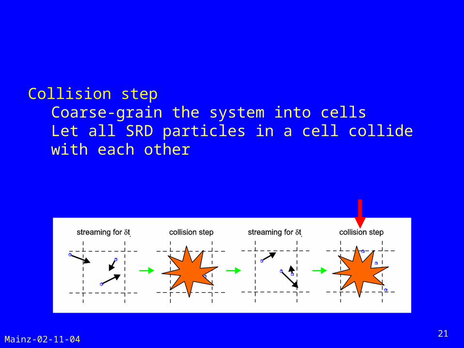
Collision stepCoarse-grain the system into cellsLet all SRD particles in a cell collide with each other

Mainz-02-11-0420

Streaming step:

2

2i

i

d rm Fdt

F ma

Mainz-02-11-0421

Collision stepCoarse-grain the system into cellsLet all SRD particles in a cell collide with each other

Mainz-02-11-0422

0(N) Coarse-grained collision step

The velocities of SRD particles, relative to the centre-of-mass velocity of each cell, are rotated around an angle.momentum and energy are locally conservedThis generates Navier Stokes hydrodynamics

/i i ii cell i cell

i i

u mv m

v u v u

Mainz-02-11-0423

A different random rotation axis for each cell;

• SRD mass m

• Rotation angle

• Cell size a

• Average density

• Temperature kT

• Collision interval t

Many parameters!

Mainz-02-11-0424

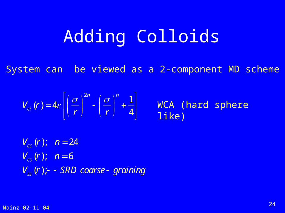
Adding Colloids

21

( ) 44

( ); 24

( ); 6

( );

n n

ci

cc

cs

ss

V rr r

V r n

V r n

V r SRD coarse graining

System can be viewed as a 2-component MD scheme

WCA (hard sphere like)

Mainz-02-11-0425

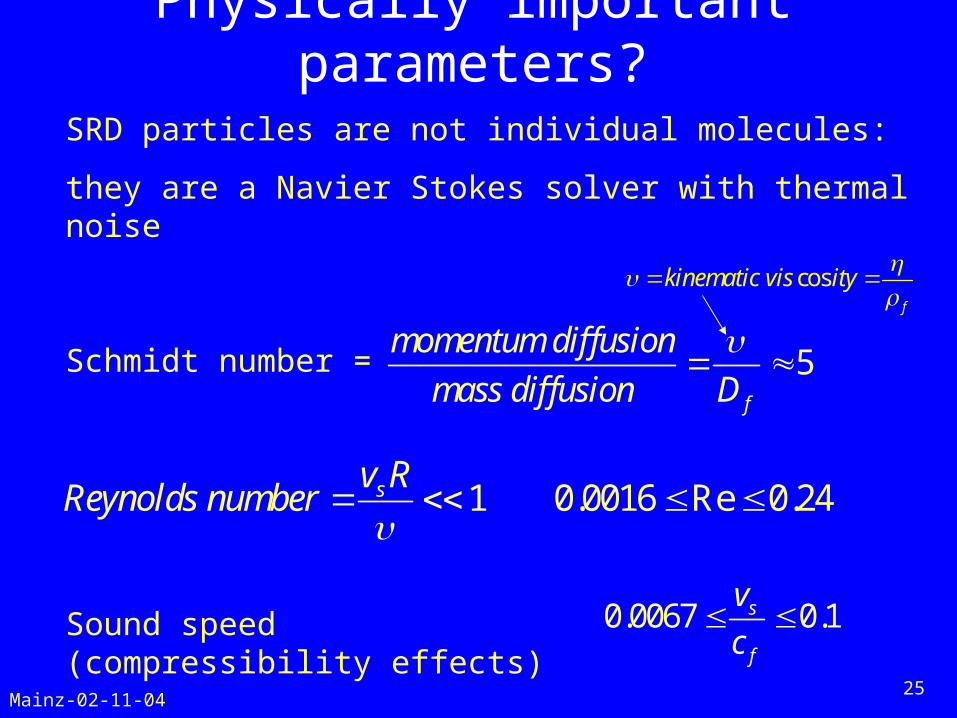
Physically important parameters?SRD particles are not individual molecules:

they are a Navier Stokes solver with thermal noise

Schmidt number = 5f

momentum diffusion

mass diffusion D

cosf

kinematic vis ity

1 0.0016 Re 0.24sv RReynolds number

Sound speed (compressibility effects)

0.0067 0.1s

f

v

c

Mainz-02-11-0426

Physically important timescales?

Solvent relaxation time: f~10-14

Brownian relaxation time: B=m/~10-9

Diffusion time D=R2/D>> B

What’s important is that they are separated

If f~SRD time-step then:

B~20 f

D~2000 f

Mainz-02-11-0427

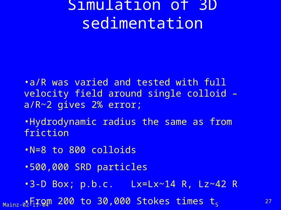
Simulation of 3D sedimentation

•a/R was varied and tested with full velocity field around single colloid – a/R~2 gives 2% error;

•Hydrodynamic radius the same as from friction

•N=8 to 800 colloids

•500,000 SRD particles

•3-D Box; p.b.c. Lx=Lx~14 R, Lz~42 R

•From 200 to 30,000 Stokes times tS

Mainz-02-11-0428

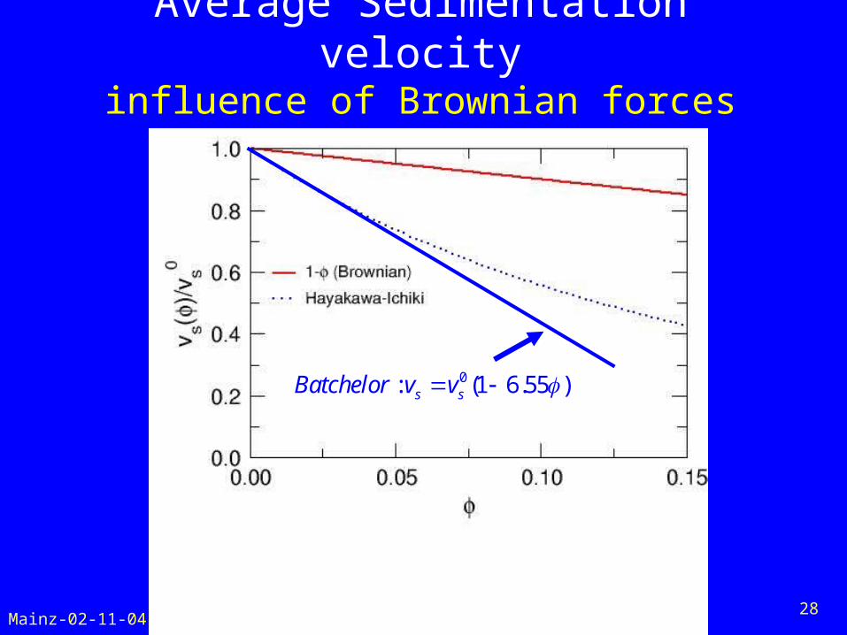
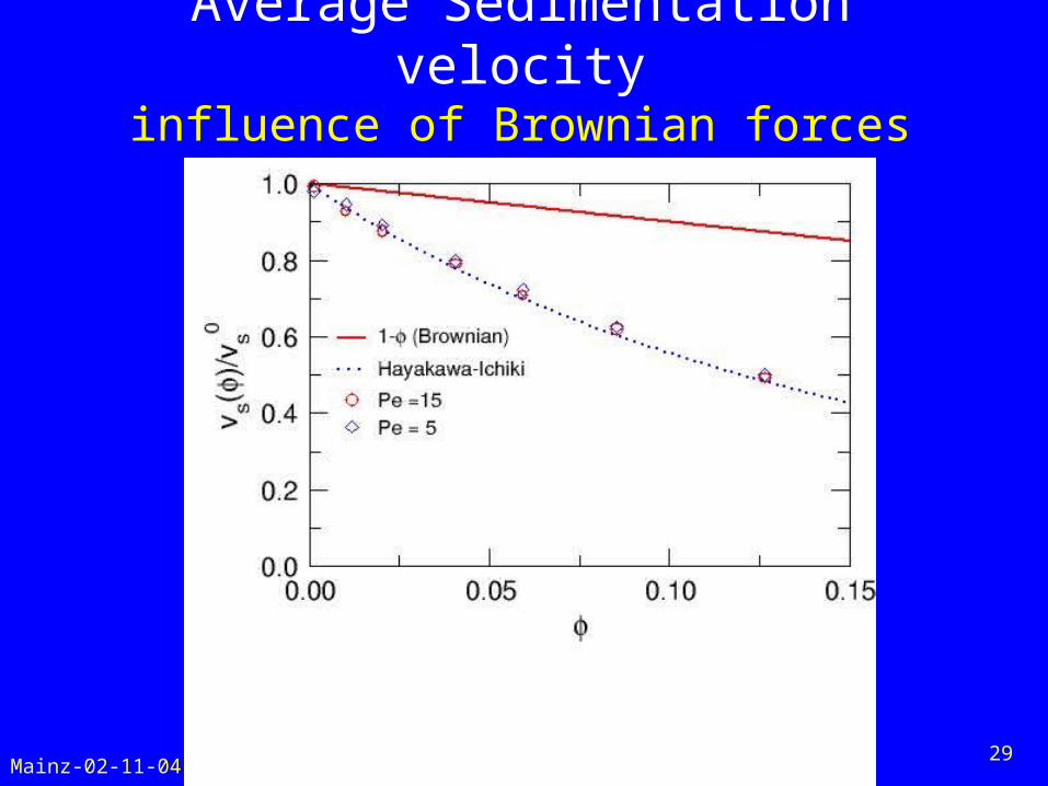
Average Sedimentation velocityinfluence of Brownian forces

0: (1 6.55 )s sBatchelor v v

Mainz-02-11-0429

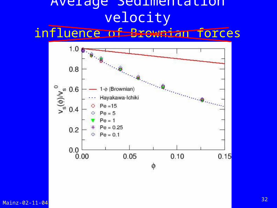
Average Sedimentation velocityinfluence of Brownian forces

Mainz-02-11-0430

Average Sedimentation velocityinfluence of Brownian forces

Mainz-02-11-0431

Average Sedimentation velocityinfluence of Brownian forces

Mainz-02-11-0432

Average Sedimentation velocityinfluence of Brownian forces

Mainz-02-11-0433

Spatial correlations

( ) (0) ( )z z zC r v v r

Swirls?

Mainz-02-11-0434

Spatial correlations

( ) (0) ( )z z zC r v v r

Scaled with (vsed)2

Swirls are dominated by hydrodynamics

Mainz-02-11-0435

Temporal Correlations:Brownian timescales

1 3/ 212 ( )f BB k T Long time tail:

( / )B Bk T t

em

Hydrodynamic fluctuations

Mainz-02-11-0436

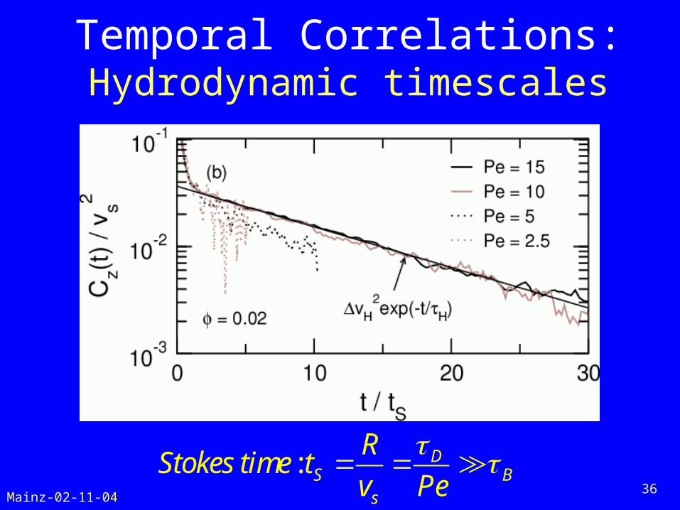
Temporal Correlations:Hydrodynamic timescales

: DS B

s

RStokes time t

v Pe

Mainz-02-11-0437

3-D sedimentation:

Average sedimentation velocity is dominated by hydrodynamics even for very small Pe (is this surprising?)

Short time fluctuations dominated by Brownian forces, but long time fluctuations by hydrodynamics for a wide range of Pe (ex of Pe*=30000)

For Pe>5 long time non-equilibrium fluctuations behave just like infinite Pe limit

Neither Brownian nor hydrodynamic interactions can be ignored

See J.T. Padding and A.A.L, cond-mat/0409133 or PRL (to appear)

Mainz-02-11-0438

Other fun things to try? We now have a flexible method to

do simulations

Mainz-02-11-0439

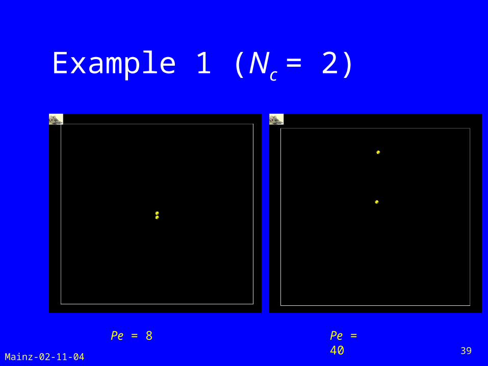
Example 1 (Nc = 2)

Pe = 8 Pe = 40

Mainz-02-11-0440

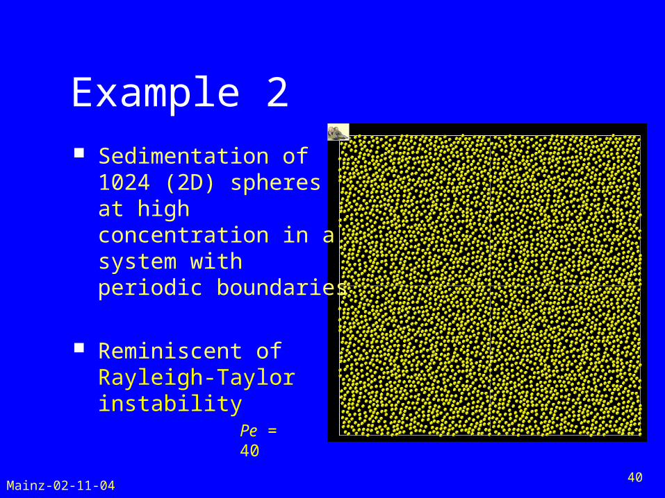
Example 2 Sedimentation of

1024 (2D) spheres at high concentration in a system with periodic boundaries

Reminiscent of Rayleigh-Taylor instability

Pe = 40

Mainz-02-11-0441

Example 3: Lane formationPe ~ 50: Brownian Dynamics Pe~50: SRD

Mainz-02-11-0442

Credits:

Person who did the work: Dr. Johan Padding Details of sedimentation:

cond-mat/0409133 – to appear PRL (2004) www-louis.ch.cam.ac.ukFor more stuff + if you’d like to join us Thank you for listening

Mainz-02-11-0443