MAGNETOCALORIC REFRIGERATION RESEARCH AT THE INCT IN...

Proceedings of the ENCIT 2014Copyright c© 2014 by ABCM

15th Brazilian Congress of Thermal Sciences and EngineeringNovember 10-13, 2014, Belém, PA, Brazil

MAGNETOCALORIC REFRIGERATION RESEARCH AT THEINCT IN COOLING AND THERMOPHYSICS

Jader Barbosa Jr., [email protected] Lozano, [email protected] Trevizoli, [email protected] - Research Laboratories for Emerging Technologies in Cooling and Thermophysics, Department of Mechanical Engineering,Federal University of Santa Catarina, Florianopolis, SC, 88040-900, Brazil

Abstract. We address the latest developments in magnetocaloric refrigeration by our research group at the NationalInstitute of Science and Technology (INCT) in Cooling and Thermophysics at the Federal University of Santa Catarina.The research activities are divided into three parts related to (i) the experimental characterization of the magnetocaloriceffect in magnetic materials, (ii) the development of mathematical models for heat transfer, fluid flow and geometricaloptimization of active magnetocaloric regenerators and (iii) the development of magnetic refrigerator prototypes and testfacilities to evaluate the performance of regenerative geometries.

Keywords: Magnetic refrigeration, magnetocaloric effect, experimental analysis, numerical modeling

1. INTRODUCTION

The magnetocaloric effect is the thermal response of a magnetic material when subjected to a changing magneticfield. Magnetocaloric refrigeration harvests the magnetocaloric effect in a regenerative thermodynamic cycle to transferheat from a low-temperature environment to a high-temperature one by means of magnetic work. The main advantage ofmagnetocaloric refrigeration compared to well-established vapor compression technologies is that the former is based oninternally-reversible thermodynamic cycles (i.e., Brayton, Stirling, Ericsson), while the latter are based on an internallyirreversible cycle (Standard vapor compression or Reversed Rankine cycle). The magnetocaloric effect is also reversiblein some materials used as solid refrigerants in magnetic cooling cycles (including gadolinium, Gd, and other alloys).

In principle, permanent magnet arrangements allow for a recovery of the magnetic work needed to magnetize the solidrefrigerant. This reduction of the required work input makes the theoretical potential for large efficiency of magneticrefrigeration very attractive. Other advantages of magnetic cooling include: (i) the absence of harmful gases such asozone depleting chemicals (CFCs), hazardous substances (NH3) or greenhouse gases (HCFCs and HFCs); (ii) morecompact layouts since the working material (i.e., refrigerant) is a solid; and (iii) less noise generation due to a reducednumber of moving parts.

The discovery of the magnetocaloric effect in the early 1900’s can be attributed to Weiss and Piccard (Smith, 2013),but the research on magnetic refrigeration for near room temperature applications started only with the first magneticcooler prototype developed by Brown (1976). Two decades later, a breakthrough paper on the discovery of the giantmagnetocaloric effect of Gd5Si2Ge2 was published by Pecharsky and Gschneidner (1997). Since then, a number oflaboratory demonstration prototypes have been reported in the literature (Gschneidner and Pecharsky, 2008; Yu et al.,2010).

Despite the potential benefits of magnetic refrigeration as an emerging cooling technology, its true gains are yet tobe fully verified for near room temperature applications. Commercial prototypes are yet to be developed, and some ofthe challenges associated with the technology involve (i) the investigation of new magnetocaloric working materials,(ii) new permanent magnet configurations and (iii) the development of new active magnetic regenerator geometries forwhich a substantial knowledge of the conjugate heat transfer and fluid flow in a porous matrix is essential for achievingan optimum design of the cooling system (Engelbrecht and Pryds, 2014). These three fronts are being advanced in ourresearch group at the INCT in Cooling and Thermophysics with the purpose of designing a new rotary magnetocaloricrefrigerator prototype. The objective of this paper is to provide an overview of our research.

The paper is divided into four parts. Firstly, the basic thermodynamics of magnetocaloric refrigeration is reviewed.Secondly, our efforts to quantify experimentally the adiabatic temperature change of promising magnetocaloric materialsvia the so-called direct method are presented. Thirdly, the mathematical modeling of the heat transfer and fluid flow in ac-tive magnetic regenerators (AMRs) is discussed. Finally, experimental analyses involving the performance of regeneratorsand the development of a rotary magnetic cooling prototype are presented.



2. FUNDAMENTALS

2.1 Thermodynamics of magnetocaloric refrigeration

A detailed introduction to the thermodynamics of magnetocaloric systems can be found in Kitanovski and Egolf(2006) and Smith et al. (2012). Here, only the fundamental aspects are reviewed so as to define the most relevantpractical parameters, namely, the isothermal entropy change and the adiabatic temperature change. At constant pressureand volume, the change in Gibbs free energy of a magnetocaloric material can be derived from:

−dG = SdT +MdH =

(∂G

∂T

)H

dT +

(∂G

∂H

)T

dH (1)

where M is the magnetization and H is the magnetic field. Entropy and magnetization are related by the followingMaxwell relationship:

(∂S

∂H

)T

=

(∂M

∂T

)H

(2)

Integration of the above equation results in a relationship for the entropy as a function of temperature and magneticfield as follows:

∆S =

∫ H2

H1

(∂M

∂T

)H

dH (3)

Entropy can also be written in terms of the specific heat capacity as follows:

(∂S

∂T

)H

=C (H,T )

T(4)

It follows that Eq. (4) can be integrated to find the entropy change if the specific heat capacity as a function oftemperature and magnetic field is known. For zero field (H = 0) and arbitrary non-zero fields (H 6= 0), one has:

S (T )H=0 − S (0)H=0 =

∫ T

0

C (H = 0, T )

TdT (5)

S (T )H − S (0)H =

∫ T

0

C (H,T )

TdT (6)

or:

∆S = S (T )H − S (T )H=0 =

∫ T

0

1

T[C (H,T )− C (H = 0, T )] dT (7)

It should be noted that Eqs. (3) and (7) represent two ways of determining the entropy change of a magnetocaloricmaterial as a function of temperature and magnetic field. A suitable engineering approximation for the majority ofmagnetocaloric materials is to assume that the specific entropy of the material is a combination of magnetic, latticeand electronic parts (Kitanovski and Egolf, 2006). While the lattice and electronic parts are assumed to depend onlyon temperature, the magnetic entropy variation depends on both the temperature and magnetic field. Thus, at constanttemperature:

∆SM ≈ ∆S = S (H2, T1)− S (H1, T1) (8)

where ∆SM is the isothermal entropy change.



At constant pressure and volume, entropy can be written in terms of temperature and magnetic field as follows:

dS =

(∂S

∂T

)H

dT +

(∂S

∂H

)T

dH (9)

Substituting Eqs. (2) and (4), for an adiabatic reversible process, one has:

dT = − T

C (H,T )

(∂M

∂T

)dH (10)

Integrating Eq. (10) gives the adiabatic temperature change:

∆Tad = −∫ H2

H1

T

C (H,T )

(∂M

∂T

)dH (11)

∆Tad = T (S (H1))− T (S (H2)) = −∫ H2

H1

T

C (H,T )

(∂M

∂T

)dH (12)

Isothermal and adiabatic magnetization and demagnetization processes are basic to a number of thermodynamic mag-netic cycles, such as the Ericsson and Brayton cycles. Figure 1 illustrates the isothermal and adiabatic magnetizationprocesses in a T -S diagram.

Temperature, T (a.u.)

Entro

py, S

(a.u

.)

Figure 1. Illustration of isothermal and adiabatic magnetization processes in a temperature-entropy diagram.

The isothermal entropy change can be calculated from measurements of magnetization as a function of temperature andmagnetic field using SQUID (Superconducting Quantum Interference Device), PPMS (Physical Property MeasurementSystem) or VSM (Vibrating Sample Magnetometer) devices (Eq. 3). Alternatively, the entropy change can be determinedvia measurements of the specific heat capacity using scanning or adiabatic calorimeters (Eq. 7). The adiabatic temperaturechange can be determined from Eq. (12) (the so-called indirect approach) or via the direct measurement approach, whichconsists of measuring the temperature change in an sample subjected to a change in magnetic field. This measurement canbe performed via temperature detectors, such as thermocouples or infrared thermography (Christensen et al., 2010). Whilethe indirect techniques require complex and sophisticated equipment — and quasi-static conditions to avoid deviation fromthermodynamic equilibrium — direct measurement can be performed more straightforwardly. Some magnetic materialsexhibit a significant MCE at near room temperature, such as gadolinium (Gd), La-based compounds (La(Fe,Si)13H)(Fujieda et al., 2004) or manganese-based compounds MnFe(P,As) (Tegus et al., 2002), which makes them potentialcandidates as refrigerants in AMR devices.



2.2 The AMR cycle

As mentioned above, a magnetic refrigerator can be designed according to a number of thermodynamic cycles. Theso-called active magnetic regenerator (AMR) cycle has received some attention in the literature for near room temperatureapplications. In an AMR refrigerator, the solid matrix is composed by a magnetocaloric material (solid refrigerant), whosetemperature is changed as a result of the magnetocaloric effect. In a cold blow, the heat transfer fluid flows through amagnetized matrix which is locally hotter than the fluid. Conversely, in a hot blow, the demagnetized matrix is cooler thanthe flowing fluid. These two processes are repeated in a cycle, thus establishing a temperature profile along the length ofthe matrix (Shah and Sekulic, 2003; Nellis and Klein, 2009; Schmidt and Willmott, 1981). The magnetic cooling systemexplored in this review is based on the thermo-magnetic Brayton cycle, presented schematically in a T -S diagram in Fig.2, which consists of the following idealized steps (Rowe et al., 2005; Kitanovski and Egolf, 2006):

1. Adiabatic magnetization: by increasing adiabatically the magnetic field applied on the matrix, the total entropy ofthe magnetic solid remains constant. However, the magnetic entropy decrease due to the magnetic field variation iscompensated by an increase in the lattice and electronic entropy contributions. As a result, the temperature of themagnetic material increases.

2. Constant magnetic field cold blow: after the adiabatic magnetization, cold fluid (at TCHEX ) flows through thematrix, cools down the solid phase (which releases heat to the fluid) and rejects heat to a hot source at THHEX .

3. Adiabatic demagnetization: similarly to the adiabatic magnetization, the demagnetization process reduces the tem-perature of the solid material, which undergoes an adiabatic temperature change.

4. Constant magnetic field hot blow: hot fluid (at THHEX ) returns through the matrix, and the solid phase removesheat from the fluid phase, increasing the internal energy of the matrix. At the cold end, the fluid absorbs heat froma cold source at TCHEX .

The efficiency of a magnetic active cooling system depends on the magnitude of the MCE (refrigerating effect) and onthe effectiveness of the regenerative matrix. The MCE itself depends on the applied field change, i.e., the higher the fieldvariation the higher the MCE, and on the magnetic properties of the magnetic material. The effectiveness, in turn, dependson the solid phase thermophysical properties, matrix geometry, thermal capacity, porosity and operating parameters, suchas frequency and flow velocity (Rowe et al., 2005; Tura and Rowe, 2011; Nielsen et al., 2012).

3. EXPERIMENTAL CHARACTERIZATION OF THE MAGNETOCALORIC EFFECT

3.1 Experimental apparatus and procedure

As mentioned above, the so-called direct approach to characterize the magnetocaloric effect is less expensive andsimpler in terms of experimentation and data analysis than the indirect approach. Moreover, depending on the natureof the experimental procedure of the direct method, adiabatic and quasi-static conditions (compulsory in the indirectapproach) need not to be fulfilled. This ensures more realistic results from the point of view of the application in arefrigeration system, since it is likely that, in this case, there will be heat transfer to or from the solid refrigerant over afinite amount of time.

Different methods and apparatuses for direct measurement of ∆Tad have been reported in literature. The main dif-ference between is related to how the magnetic field is generated. Some devices make use of an electromagnet (Zhanget al., 2000; Canepa et al., 2005), others superconductor coils (Benford and Brown, 1981; Gopal et al., 1997; Gschneidnerand Pecharsky, 2000; Rosca et al., 2010) and, most recently, permanent magnet assemblies (Huang et al., 2005; Trevizoliet al., 2009, 2012; Madireddi et al., 2009; Bahl and Nielsen, 2009; Khovaylo et al., 2010).

An experimental apparatus has been designed and constructed for directly measuring the MCE of promising magne-tocaloric materials (Fig. 3). The magnetic field is provided by a Nd2Fe14B Halbach permanent magnet assembly with avolume of uniform magnetic flux density of 1.75 T. A pneumatic actuator with a nylon arm is used to traverse the sampleinto and out of the magnet with a change of magnetic field of the order of milliseconds.

Magnetic refrigerant samples in bulk or powder form can be characterized. Bulk form samples are shaped from tworectangular plates and between them a thin T-type thermocouple is carefully placed to enable the characterization of themagnetic temperature change. The thermocouple tip is positioned in the center of the gap between the plates and, toimprove thermal contact, the gap is filled with a thin layer of a high-density ceramic-base thermal grease to minimize theinterference with the magnetic field. The samples were thermally insulated with a 5-mm layer of expanded polystyrene,as seen in Fig. 4. The apparatus is placed inside a 29-liter thermally insulated chamber in which the temperature control isperformed via a combination of Peltier modules and a copper coil heat exchanger connected to a temperature-controlledthermal bath. The system is capable of operating at temperatures between 250 and 350 K controlled to within ± 0.05 K.



Figure 2. Schematic description of the processes in a thermo-magnetic Brayton cycle

Figure 3. Apparatus to measure the magnetocaloric effect via the direct method.

A typical measurement of the magnetocaloric temperature change consists of the following steps. Once the samplestabilizes at the desired temperature, a solenoid valve activates the pneumatic actuator placing the sample inside themagnet, which causes an instantaneous change of the magnetic field in the sample from 0 to 1.75 T (magnetization). Thesample stays in the magnetic field for a few seconds before the solenoid valve is closed and the sample is moved out ofthe magnetic field (demagnetization). Fig. 5 shows the results of a typical measurement, which consists of three steps:



(a) Step-by-step preparation of a sample for the direct measurements. (b) Sample with the polystyrene insulation. .

Figure 4. Sample preparation.

temperature stabilization before (de)magnetization, the (de)magnetization process (with initiates with a thermocouplesignal interference due to the magnetic field change) and finally the (de)magnetization. This measurement procedureis repeated five times for each desired temperature to guarantee reproducibility and decrease experimental uncertainty,which was calculated as 0.20 K.

81.50 81.75 82.00 82.25 84.00 84.25 84.50 84.75282

284

286

288

290

Tem

pera

ture

[K]

Time [s]

Magnetization Demagnetization

Figure 5. Typical experimental result of the temperature variation due to magnetization and demagnetization of a sample.

The adiabatic temperature change is taken as the difference between the average plateau temperatures of the samplewhen it is out and in the magnetic field. The temperature fluctuations (spikes) due to the magnetic induction of thethermocouple when it is moving in the field have been excluded from the averaging. The influence of the sample shape onthe magnetic field is taken into consideration through the sample demagnetization factor, ND. For prismatic bodies, thedemagnetization factor can be calculated according to the algebraic relationships of Aharoni (1998). ND is responsible forreducing the intensity of internal magnetic field, Hint, in comparison with the applied magnetic field. For an isothermalsample, ND is calculated as (Bahl and Nielsen, 2009; Smith et al., 2010):

Hint = Happ −NDM (13)

where Happ corresponds to the applied magnetic field. In the present measurements, µ0Happ = 1.75 T and µ0 is thepermeability of free space.



3.2 Direct measurement results

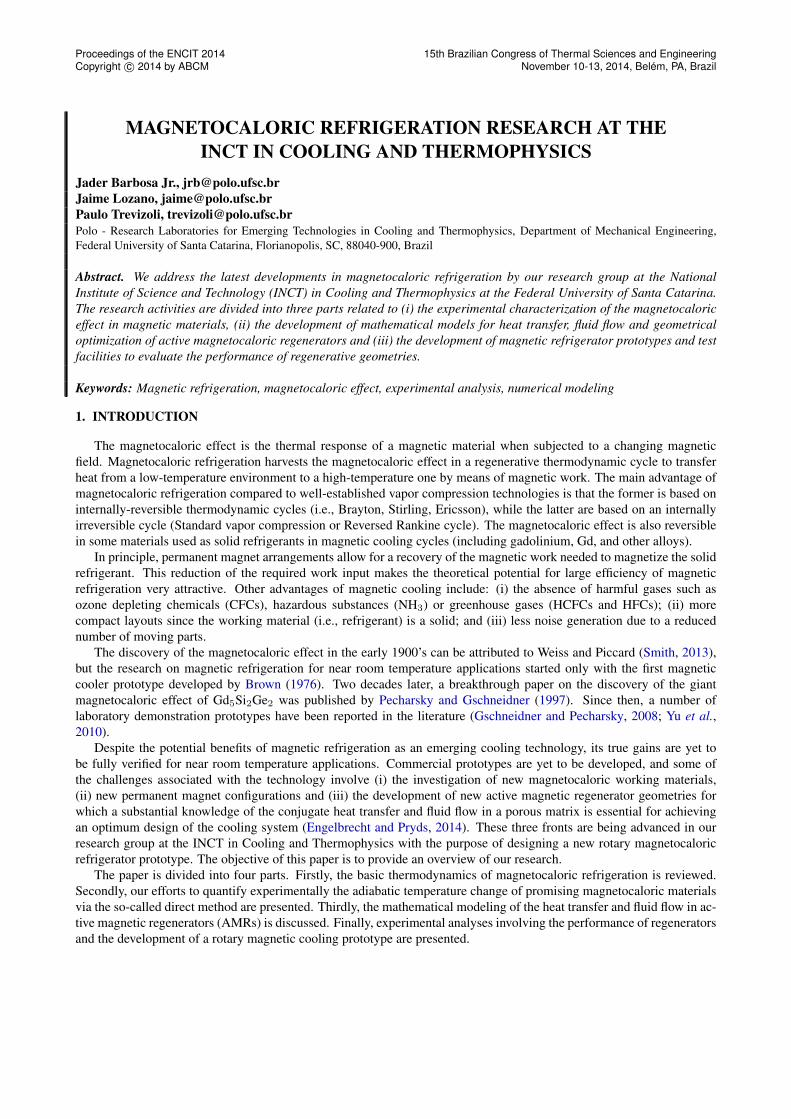
Preliminary experimental results were generated for gadolinium (Gd) samples (Trevizoli et al., 2012) as a means ofvalidating the experimental apparatus and procedure. Typical results for Gd are shown in Fig. 6. for ∆Tad as a functionof temperature for magnetization and demagnetization (the ND of the sample was 0.687). A distinct temperature shiftis observed between the curves, with the peaks of the curves taking place at around 293 K for magnetization and 297 Kfor demagnetization. This result can be explained on the grounds of the reversibility of MCE under conditions of zeroheat transfer. Neglecting any kind of internal irreversibility (homogeneous material, uniform temperature variations),the system is expected to perform a cycle and return to the original state (i.e., zero total entropy variation) with zeroentropy generation. The shift of the demagnetization curve with respect to that for magnetization is a consequence of thisconstraint. For materials with a continuous adiabatic temperature change, such as Gd, it follows that,

∆Tad,mag (T1, H1, H2) = −∆Tad,demag (T1 + ∆Tad,mag (T1, H1, H2) , H1, H2) (14)

In other words, when a magnetized material is demagnetized from a starting temperature T2 > T1, it will cool to aunique temperature T1 which obeys T2 = T1 + ∆Tad,mag (T1, H1, H2) (Nielsen et al., 2010a). Figure 6 shows a com-parison between ∆Tad,demag calculated via Eq. (14) and ∆Tad,demag obtained experimentally. An excellent agreementis observed.

280 285 290 295 300 3052.0

2.2

2.4

2.6

2.8

3.0

3.2

3.4

3.6

3.8

4.0ND = 0.687

Tad,mag (K) Tad,demag (K) Theoretical

T ad

(K)

Temperature (K)

Figure 6. Validation of the experimental method using gadolinium low magnetic fields (< 2 T).

Direct measurements were also carried out of for MnFe(P,As) samples. Figure 7 shows the magnetization and demag-netization curves for a sample subjected to heating (increasing temperature) and cooling (decreasing temperature) ramps.Since Mn-based compounds undergo a first-order transition, a thermal hysteresis is expected to occur around the transitiontemperature. In this sample, a thermal hysteresis of about 0.6 K was observed. Thermal hysteresis is, in principle, anundesirable effect in the context of the application of these materials in AMR devices and a more detailed study of thiseffect in these compounds is presented by von Moos et al. (2014). Before acquiring the data shown in Fig. 7, the samplewas subjected to heating-cooling thermal cycles to elminate training effects.

One of the main advantages of manganese-based compounds is the possibility of tuning its TC , which facilitates theconstruction of multi-layer AMRs to reach larger temperature spans in the regenerator. Figure 8 shows the adiabatic tem-perature change of samples with different compositions and different Curie temperatures. The difference in the adiabatictemperature change between the samples is due to the distinct values of ND for each sample.

4. MATHEMATICAL MODELING OF ACTIVE MAGNETOCALORIC REGENERATORS

4.1 Fluid flow and heat transfer

A recent review of the state of the art in mathematical modeling of AMRs has been conducted by Nielsen et al.(2011). In our group, multi-dimensional approaches (2D and 3D) have been pursued in the works of Oliveira et al.(2009a,b, 2012) and Canesin et al. (2012) for parallel-plate regenerator geometries. The works of Oliveira et al. advanced



µ0H = 1.75 T

272 276 280 284 288 292 2960.0

0.5

1.0

1.5

2.0

2.5

3.0 Mn-2ND=0.58

ΔT ad

[K]

Temperature [K]

ΔTad,mag,cooling

- ΔTad,demag,cooling

ΔTad,mag,heating

- ΔTad,demag,heating

Figure 7. Thermal hysteresis in the heating and cooling of a MnFe(P,As) sample.

270 280 290 300 310 320 3300.0

0.5

1.0

1.5

2.0

2.5

3.0

3.5

4.0

ΔT ad

[K]

Temperature [K]

Mn-1 (ND=0.46)

Mn-2 (ND=0.58)

Mn-3 (ND=0.56)

Heating

Figure 8. Adiabatic temperature change of three MnFe(P,As) samples with different compositions when submitted underan applied magnetic field of 1.75 T.

a hybrid approach for solving the parallel-plate AMR geometry, which consisted of an analytical solution of the oscillatingflow field and a finite-volume numerical solution of the conjugate heat transfer in the solid and fluid phases. It has beenshown that for values of the kinetic Reynolds number below 3.5, the effect of frequency on the interstitial heat transfercoefficient was small, i.e., there was a small deviation (lower than 10%) between the oscillating and steady-state valuesof the Nusselt number. A kinetic Reynolds number of 3.5 corresponded to operating frequencies that are much higher(in excess of 10 Hz) than those currently utilized in experimental AMRs. For this reason, one-dimensional models (withsteady-state closure relationships for fluid friction and interstitial heat transfer) appear to be adequate for the description



of the oscillatory fluid flow and heat transfer in AMRs.The one-dimensional mathematical model developed for the thermal-hydraulic analysis of regenerators is presented in

detail in Trevizoli et al. (2014c). The study was focused on regenerative geometries consisting of a bed of speherical Gdparticles. The momentum balance for laminar, incompressible flow in a low porosity medium with negligible body forcesis given by,

ρfε

(∂u

∂t

)= −∂p

∂z− µfKu− cEρf

K1/2|u|u (15)

where ρf is the fluid density, ε is the porosity, u is the fluid velocity, p is the pressure and µf is the fluid dynamic viscosity.K is the permeability and cE is the Ergun constant for beds of spheres given by Kaviany (1995),

K =ε3

180(1− ε)2d2p (16)

cE =1.8

(180ε3)0.5 (17)

where dp is the particle diameter.The oscillatory (sinusoidal) flow in the regenerator is described by a time-dependent pressure gradient as follows

(Zhao and Cheng, 1998; Oliveira et al., 2012),

−∂p∂z

= ρfAt sin(2πft) (18)

whereAt is the amplitude of the fluid flow waveform and f is the cycle frequency. The energy equation for the fluid phaseis given by,

ε∂Tf∂t

+ u∂Tf∂z

= − hβ

ρfcp,f(Tf − Ts) + ε

κdρfcp,f

∂2Tf∂z2

+1

ρfcp,f

∣∣∣∣∣∂p∂z u∣∣∣∣∣ (19)

where the terms on the left are the due to transient and advection effects, and those on the right are due to interstitialheat transfer between the solid and the fluid, axial conduction/dispersion (Kaviany, 1995) and viscous dissipation. Theinterstitial heat transfer coefficient, h, was calculated using the Whitaker correlation (Kaviany, 1995). The energy equationfor the solid phase is given by,

(1− ε)∂Ts∂t

= − hβ

ρscs(Ts − Tf ) + (1− ε) κst

ρscs

∂2Ts∂z2

(20)

where the solid static thermal conductivity, κst, was calculated using the Hadley correlation (Kaviany, 1995). The mag-netocaloric effect was implemented via the so-called direct approach (Nielsen et al., 2011), which consists of a directtemperature increment (or reduction) during the magnetization (or demagnetization) step. For a one-dimensional domain,

Ts(t+ ∆t, z) = Ts(t, z) + ∆Tad(∆H,Ts(t, z)) (21)

where the adiabatic temperature change was calculated via the Weiss-Debye-Sommerfeld (WDS) theory, which accountsfor the magnetic, lattice and electronic contributions to the total entropy change (Morrish, 1965). Thus,

∆Tad(∆H,Ts(t, z)) = −Ts(t, z)cs(t, z)

∆ss(∆H,Ts(t, z)) (22)

The governing equations for the fluid and solid phases were solved using the finite volume method (FVM) with a fullyimplicit scheme. Further details can be found in Trevizoli et al. (2014c).



4.2 Entropy generation

The entropy generation in the 1-D regenerator model is due to heat transfer between solid and fluid phases, axial heatconduction in the fluid and solid phases and viscous dissipation in the fluid. Therefore, the rate of entropy change in acontrol volume containing both the solid and fluid phases is given by Steijaert (1999),

dS

dt= −(1− ε)Ac

[d

dz

(q′′AC,sTs

)dz

]s

− εAc

[d

dz

(q′′AC,fTf

)dz

]f

+ mds

dzdz + S

′′′

g Acdz (23)

where the first and second terms on the right are changes in entropy rate due to axial conduction heat transfer in the solidand fluid. The third term is the rate of entropy change associated with the fluid flow into and out of the control volume.The fourth term is the rate of entropy generation in the control volume. The rate of entropy change in the control volumeis the sum of the entropy changes in the fluid and solid phases,

dS

dt=dS

dt

∣∣∣∣∣f

+dS

dt

∣∣∣∣∣s

(24)

where the rates of entropy change in the fluid and solid are given by (Steijaert, 1999),

dS

dt

∣∣∣∣∣f

= −εAcTf

[dq′′AC,fdz

dz

]f

+q′′HTTf

Acdz + mds

dzdz +

1

ρfTf

∣∣∣∣∣m(−dpdz

)∣∣∣∣∣dz (25)

dS

dt

∣∣∣∣∣s

= − (1− ε)AcTs

[dq′′AC,sdz

dz

]s

− q′′HTTs

Acdz (26)

where q′′AC,f = κddTf/dz and q′′AC,s = κstdTs/dz are the axial heat fluxes in the liquid and solid domains. q′′HT =hβ(Ts − Tf ) is the heat transfer rate per unit surface area between the fluid and solid phases.

Combining Eqs. (23)-(26) and Eq. (24), the local rate of entropy generation per unit volume is given by,

S′′′

g =hβ(Ts − Tf )2

TsTf+εκfT 2f

(dTfdz

)2

+(1− ε)κst

T 2s

(dTsdz

)2

+1

Tf

∣∣∣∣∣uD(−dpdz

)∣∣∣∣∣ (27)

where the first term on the right is the entropy generation rate per unit volume due to interphase heat transfer with a finitetemperature difference. The second and third terms are the entropy generation rate due to axial conduction in the fluidand solid matrix, and the fourth term is the entropy generation rate per unit volume due to viscous friction. The entropygeneration in the regenerator during a cycle, Sg , is calculated by (in J/K),

Sg = Ac

∫ L

0

∫ τ

0

S′′′

g dt dz (28)

Sg is used as the objective function to be minimized in the regenerator optimization described next.

4.3 Model results

4.3.1 Evaluation of the influence of the magnetic field waveform and model validation

Trevizoli et al. (2014c) used the model described above to evaluate the effect of the applied magnetic field waveform(instantaneous change, sinusoidal change and rectified sinusoidal change) and of demagnetizing effects on the perfor-mance of an AMR containing spherical Gd particles. The instantaneous waveform is the ideal waveform of the thermo-magnetic Brayton cycle, for which the changes between the minimum and maximum values of magnetic induction occurinstantly. For this reason, it cannot be implemented in practice, but is the easiest waveform to simulate numerically,and most theoretical works published so far use this kind of applied field behavior in their simulations of AMR systems(Nielsen et al., 2011).



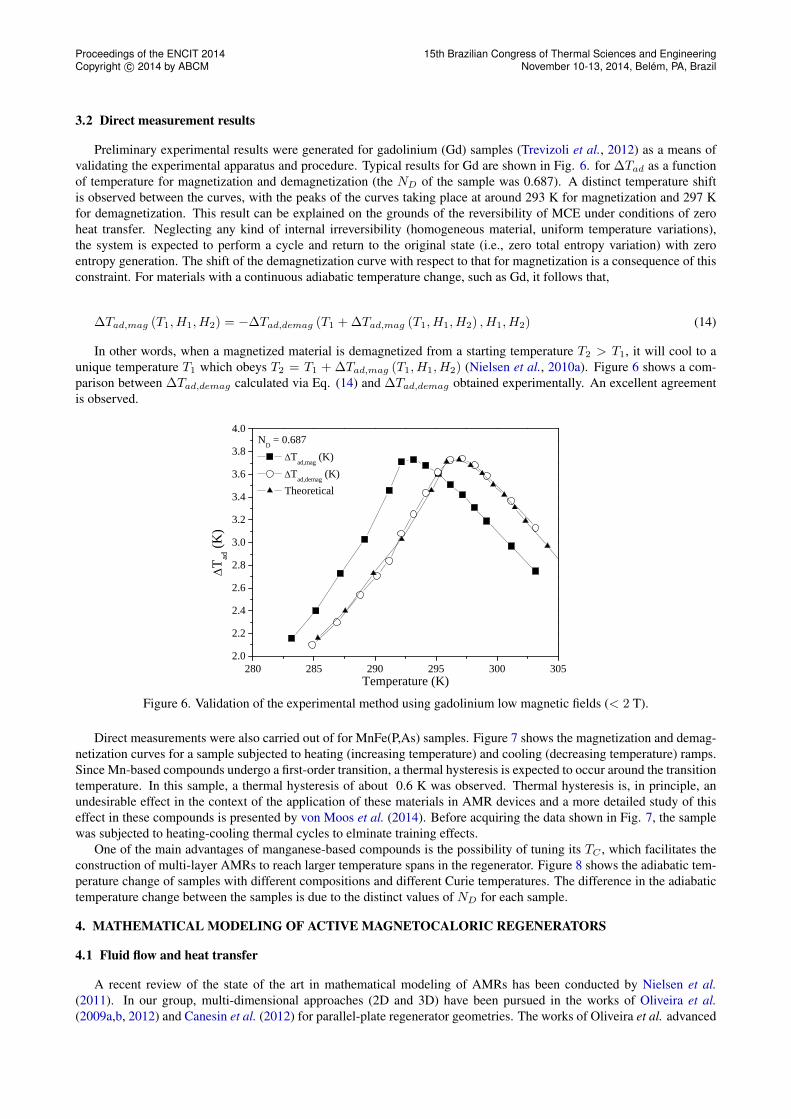
The data used to evaluate the model were associated with an experimental facility described in detail by Arnold et al.(2014) and Trevizoli et al. (2014c). The setup is composed by two regenerators filled with 0.5-mm Gd spheres and twonested (concentric) cylindrical Halbach arrays dephased by 180◦. The length of the regenerators was 150 mm and theirhydraulic diameter was 22.1 mm. The maximum magnetic field measured experimentally in the nested configuration was1.4 T, while the minimum was about 0.06 T (Arnold et al., 2014). The working fluid was a water-glycol mixture (20%vol.). The fluid displacement was described by a sinusoidal waveform, which was in phase with the applied magnetic fieldwaveform. The temperature in the hot heat exchanger was controlled by water chiller, while the cold heat exchanger wasa Joule heater to emulate the applied thermal load.

The maximum calculated regenerator temperature span (at zero thermal load), ∆Tspan,max, and the cooling capacitiesassociated with specified temperature spans were higher for the instantaneous waveform. This behavior was more orless independent of the hot-side temperature, THHEX . For instance, at zero thermal load, ∆Tspan,max for the instanta-neous waveform was roughly 5 K higher than for the sinusoidal waveform. The sinusoidal waveform, in turn, exhibitedtemperature spans roughly 3-4 K larger than those of the rectified sinusoidal waveform.

A cooling load curve (∆Tspan vs. cooling capacity) is presented in Fig. 9 for THHEX = 295 K. The results show that∆Tspan increases with THHEX and that the instantaneous waveform has the highest cycle-average cooling capacity, withvalues 20%-60% higher than the sinusoidal waveform. The cycle-average cooling capacity for the rectified sinusoidalwaveform can be 20%-90% lower than that for the sinusoidal waveform. The instantaneous and cycle-average coolingcapacities are defined by:

qC = m(t)cp [TCHEX − T (t)] (29)

qC =1

τ

∫ τ

0

qCdt (30)

where T (t) is the instantaneous temperature of the fluid exiting the matrix during the hot blow and τ is the cycle period.

0 20 40 60 80 100 120 140 1600

5

10

15

20

25

30

35

40

Instantaneous Sinusoidal Rectified sinusoidal

Cooling capacity [W]

Tsp

an [K

]

0 5 10 15 20 25 3010

20

30

40

50

60

70

80

90

100 Instantaneous vs. sinusoidal sinusoidal vs. rectified sinusoidal

Red

uctio

n in

coo

ling

capa

city

[%]

Tspan [K]

Figure 9. Load numerical results for different waveforms for the hot source at 295 K.

Although the maximum temperature span and the cooling capacity are the result of interconnected transport andthermo-magnetic phenomena taking place in the regenerator matrix, it became clear from the analysis of Trevizoli et al.(2014c) that, for a sinusoidal fluid displacement waveform, the regenerator heat transfer performance improved whenthe magnetocaloric material remained for the longest time possible under a low magnetic field during the hot blow. Adetailed evaluation of the temperature distribution in the matrix as a function of time during the cycle revealed that thesinusoidal and rectified sinusoidal waveforms gave values of solid temperature which were always higher than those dueto the instantaneous waveform.

The experimental tests with an applied thermal load were performed for the following conditions: (i) stroke of 15 mm,frequency of 0.5 Hz and THHEX between 293 K and 298 K; (ii) stroke of 15 mm, frequency of 0.75 Hz and THHEX of298 K, and (iii) stroke of 20 mm, frequency of 0.75 Hz and THHEX of 298 K Arnold et al. (2014). Figure 10 shows thebehavior of the temperature span as a function of the cooling capacity for different values of the piston stroke.



0 20 40 60 80 1000

5

10

15

20

25

30

35

40

Tsp

an [K

]

Cooling capacity [W]

Experimental Str = 15 mm Experimental Str = 20 mm Numerical Str = 15 mm Numerical Str = 20 mm

Figure 10. Comparison between experimental and numerical results for tests with thermal load. Frequency of 0.75 Hz,hot source temperature of 298 K and different strokes.

As can be seen from Fig. 10, the agreement between model and experiments improves as ∆Tspan goes to zero, whichcan be justified based on the heat gain from the ambient due to insufficient thermal insulation. Additional thermal loadtests were performed in which THHEX and ∆Tspan were kept constant at 298 K and 5 K, respectively, while the stroke(or the utilization factor) and frequency were changed, as shown in Fig. 11. Again, a good agreement between numericaland experimental results was obtained at lower values of frequency.

0.2 0.3 0.4 0.5 0.6 0.70

20

40

60

80

100

120

140

Experimental - f=0.4Hz Experimental - f=0.6Hz Experimental - f=0.8Hz Numerical - f=0.4Hz Numerical - f=0.6Hz Numerical - f=0.8Hz

Coo

ling

capa

city

[W]

Utilization factor

Figure 11. Comparison between the experimental and numerical thermal load results for a hot source temperature of 298K and a temperature span of 5 K.

4.3.2 Entropy generation minimization (EGM) optimization

Trevizoli et al. (2014a) carried out numerical simulations of EGM in passive and active regenerators based on theperformance evaluation criteria (PEC) of Webb and Kim (2005). These proved to be a useful and versatile tool forregenerator design according to different constraints. In the Variable Geometry (VG) PEC, the regenerator housing crosssectional area (or housing diameter, Dh) and length, L, are allowed to vary, keeping a constant housing volume. In theFixed Face Area (FA) PEC, the housing diameter is kept constant and the regenerator length can vary, so the housingvolume is variable. While the VG PEC is useful for optimizing regenerator geometries (i.e., aspect ratios) for a fixedvolume of regenerator material, the FA PEC is indicated for assessing the effect of the length of the regenerator on the



system performance.The reference geometry for the active regenerator simulations of Trevizoli et al. (2014a) has a housing diameter of 25

mm and aspect ratio (ζ = L/Dh) of 2, resulting in a housing volume of 24.544 cm3. The ranges of values of Dh andL/Dh for the VG and FA PEC were 12.5-75 mm and 1-16, respectively. For each possible combination ofDh and L/Dh,the particle diameter, dp, was also varied. The simulations were carried out considering constraints of fixed cycle-averagecooling capacity (40 W) and ∆Tspan (15 K). The solid material was gadolinium and the heat transfer fluid was treated aswater.

Figure 12 presents the cooling capacity-entropy generation contour lines for the VG and FA PEC applied to the thermalanalysis of AMRs. Lines of constant Sg (orange lines) are plotted together with lines of constant average cooling capacity(black lines) for both PEC. The target cooling capacity of 40 W per regenerator (black solid line) can be achieved withdifferent combinations of Dh, ζ and dp, with the flow rate held constant. The response of Sg to these parameters in theAMR PEC was found to be similar to the passive case. Nevertheless, as can be seen from Fig. 12, there is more thanone regenerator configuration that satisfies the optimization constraints. For instance, in the VG PEC, for dp = 1 mm, acooling capacity of 40 W can be achieved with Dh ≈ 15 mm or with Dh ≈ 55 mm. However, the entropy generation ishigher for the latter.

-200

-150

-100

-100

-50

-50

-50

0

0

0

20

20

3030

30

40

40

50

50Particle diameter [mm]

Housingdiameter[mm]

0.25 0.5 0.75 1 1.25 1.5 1.75 2

15

20

25

30

35

40

45

50

55

60

65

70

75

0.015

0.015

0.0175

0.0175

0.0175

0.02

0.02

0.02

0.0225 0.0225

0.0225

0.0225

0.025

0.025

0.025

0.025

0.025

0.0275

0.0275

0.0275

0.0275

0.03

0.03

0.03

0.035

0.035

0.035

0.04

0.04

0.04

0.045

0.045

0.05

0.05

(a)

-300-300

-200

-200-200

-100

-100

0

0

40

40

100

100

0.0375

0.0375

0.04

0.04

0.04

0.040.

0425

0.0425

0.0425

0.0425

0.0425

0.045

0.045

0.045

0.045

0.05

0.05

0.05

0.05

0.05

0.06

0.06

0.06

0.08

0.08

0.08

0.1

0.1

0.2

Particle diameter [mm]

Aspectratio[-]

0.25 0.5 0.75 1 1.25 1.5 1.75 22

3

4

5

6

7

8

9

10

11

12

13

14

15

16

(b)

Figure 12. Average cooling capacity (black lines) and Sg (orange lines) for active regenerators as a function of: (a) Dh

and dp for PEC VG at 100 kg/h; (b) ζ and dp for PEC FA at 200 kg/h.

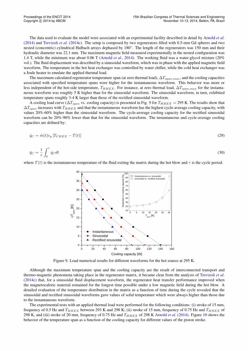
In addition to the VG and FA PEC, EGM-based simulations were carried out for the fixed geometry (FG) PEC. In thiscriterion, the dimensions of the regenerator housing are fixed and the geometry and type of the regenerative material arevaried. This PEC is useful for evaluating different matrix types, such as bed of spheres, parallel plates, screen meshes andpins (Trevizoli et al., 2014b).

In the FG analysis, the regenerator housing geometry had a face area of 169.72 mm2 and length of 100 mm in thetwo cases simulated. In the first case, the frequency, f , was set at 1 Hz, while the equivalent particle diameter, Dp, andmass flow rate, m, were variable (0.3-1.5 mm and 10-100 kg/h). The utilization factor defined as the ratio of the thermalmasses of the fluid and solid phases (Nielsen et al., 2011),

φ =mcPf

fρscPs(1− ε)AcL(31)

depended only on m, and ranged from 0.183 (10 kg/h) to 1.83 (100 kg/h). Fig. 13 presents the results for the first case,where the solid symbols are related to Sg and the open symbols to m. For a given dp associated with each geometry, thereare two values of m that satisfy the problem constraints. These become closer as dp increases, and the lowest m alwaysgives the lowest Sg for a given geometry. Considering the problem constraints and parameter ranges, the parallel-plategeometry presented the smallest Sg of all geometries, as seen in the table insert in Fig. 13. This can be attributed chieflyto the lowest viscous dissipation and small demagnetizing losses when compared with the other geometries. However,the smallest Sg is associated with a plate thickness of 0.1 mm (dp = 0.3 mm), which may not be easy to manufactureconsidering a porosity of 0.36.



Figure 13. FG PEC results for variable particle diameter and mass flow rate.

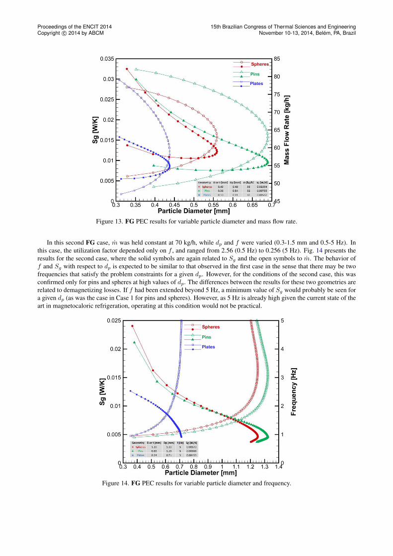
In this second FG case, m was held constant at 70 kg/h, while dp and f were varied (0.3-1.5 mm and 0.5-5 Hz). Inthis case, the utilization factor depended only on f , and ranged from 2.56 (0.5 Hz) to 0.256 (5 Hz). Fig. 14 presents theresults for the second case, where the solid symbols are again related to Sg and the open symbols to m. The behavior off and Sg with respect to dp is expected to be similar to that observed in the first case in the sense that there may be twofrequencies that satisfy the problem constraints for a given dp. However, for the conditions of the second case, this wasconfirmed only for pins and spheres at high values of dp. The differences between the results for these two geometries arerelated to demagnetizing losses. If f had been extended beyond 5 Hz, a minimum value of Sg would probably be seen fora given dp (as was the case in Case 1 for pins and spheres). However, as 5 Hz is already high given the current state of theart in magnetocaloric refrigeration, operating at this condition would not be practical.

Figure 14. FG PEC results for variable particle diameter and frequency.



5. DEVELOPMENT OF LABORATORY PROTOTYPES

5.1 First generation: Reciprocating AMR apparatus

The first laboratory prototype tested at the Federal University of Santa Catarina has been described by Trevizoli et al.(2011). The AMR experimental apparatus is shown schematically in Fig. 15 and consisted of a reciprocating systemwith a fixed regenerator and a pneumatic system to move the magnet and change the magnetic flux. The regeneratorconsisted of 28 parallel plates of commercial-grade Gd plates (160 mm long, 0.85 mm thick, 6.9 mm height), whichformed 26 parallel channels (160 mm long, 0.1 mm thick, 6.4 mm height). The total mass of Gd in the regenerator was195.4 g. The matrix porosity was 9.2 %. The regenerator housing was made of AISI 304 stainless steel, and de-ionizedwater was the heat transfer fluid. The magnetic field was generated by Nd2Fe14B permanent magnets in a Halbacharray. The (volume) average magnetic field applied on the regenerator was approximately 1.22 T (uncertainty of 3.5 %).The operating frequency was fixed at 0.14 Hz. The hot heat exchanger (HHEX) was a cross-flow mini channel copperheat exchanger. A thermoelectric module was attached to one side of the heat exchanger surface to emulate a constanttemperature hot source. The cold heat exchanger (CHEX) was an electric (Joule) heater with a constant dissipation rate.

Figure 15. Schematic diagram of the reciprocating AMR test device.

The results obtained with the reciprocating AMR test device have shown qualitative agreement with the trends reportedin the literature for tests with and without applied thermal loads. The maximum temperature difference between the hotand cold sources at zero thermal load was 4.4 K for an utilization factor of 0.4 and THHEX = 296.15 K. For tests witha thermal load, the typical linear relationship between the cooling capacity and the temperature difference between thesources has been observed. A maximum cooling capacity was achieved for an utilization factor of 0.9. In absolute andgeneral terms, the results obtained with the first lab demonstration prototype were quite modest, which can be attributedto losses of several types along the cycle. Some of the potential losses have been investigated numerically by Nielsenet al. (2010b). In these numerical simulations, the spatial variation of the magnetic field was taken into account as wasthe regenerator geometry. Considering cases with and without thermal parasitic losses, it was shown that the numericalAMR model significantly over predicted the zero load temperature span of the experiment. Given the conditions at whichthe experiments were performed, a better performance was expected. It was argued that the main cause for the lack ofperformance with the first apparatus was that the stainless steel casing acting as regenerator housing would have such alarge thermal conductivity that the regenerator in practice was “short-circuited” thermally, i.e., the thermal gradient waspartially destroyed by the housing.



5.2 Second generation: Rotary AMR prototype

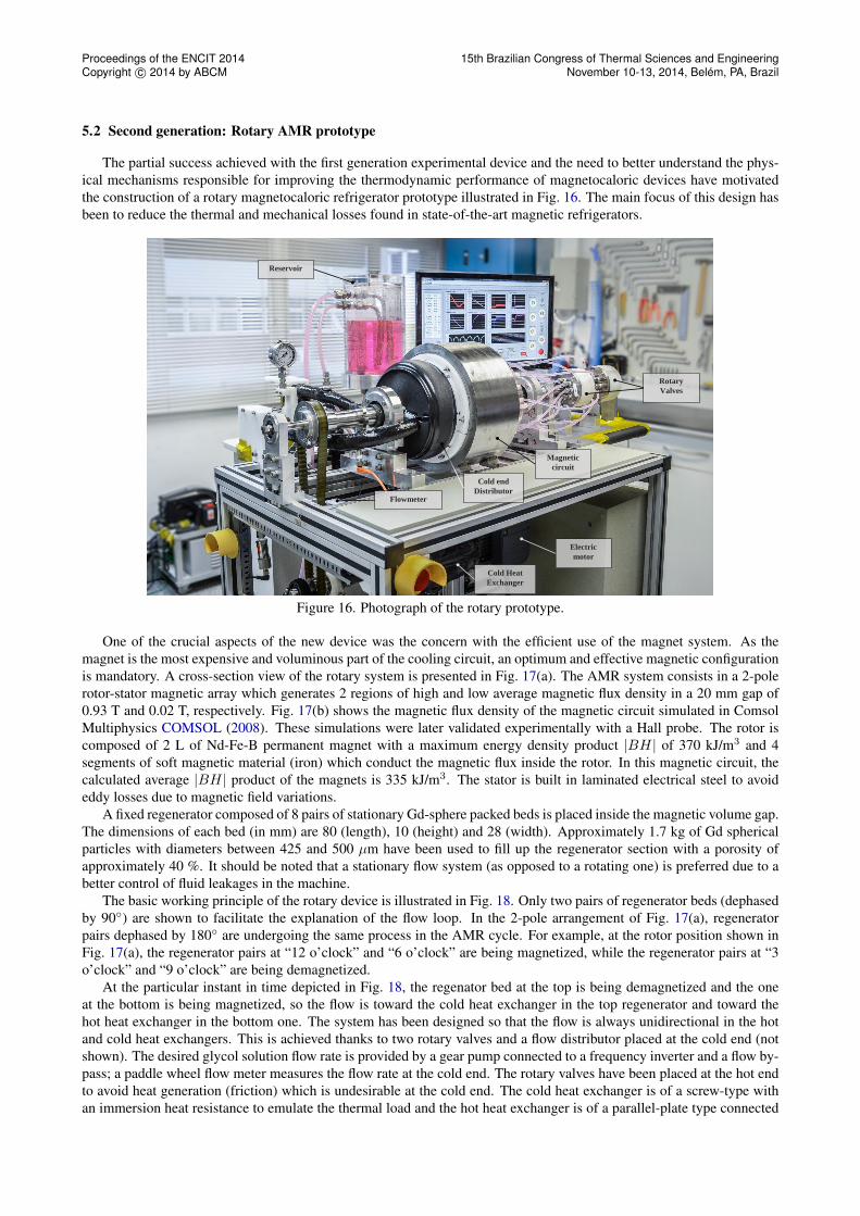
The partial success achieved with the first generation experimental device and the need to better understand the phys-ical mechanisms responsible for improving the thermodynamic performance of magnetocaloric devices have motivatedthe construction of a rotary magnetocaloric refrigerator prototype illustrated in Fig. 16. The main focus of this design hasbeen to reduce the thermal and mechanical losses found in state-of-the-art magnetic refrigerators.

Magnetic

circuit

Electric

motor

Rotary

Valves

Reservoir

Cold Heat

Exchanger

Cold end

Distributor Flowmeter

Figure 16. Photograph of the rotary prototype.

One of the crucial aspects of the new device was the concern with the efficient use of the magnet system. As themagnet is the most expensive and voluminous part of the cooling circuit, an optimum and effective magnetic configurationis mandatory. A cross-section view of the rotary system is presented in Fig. 17(a). The AMR system consists in a 2-polerotor-stator magnetic array which generates 2 regions of high and low average magnetic flux density in a 20 mm gap of0.93 T and 0.02 T, respectively. Fig. 17(b) shows the magnetic flux density of the magnetic circuit simulated in ComsolMultiphysics COMSOL (2008). These simulations were later validated experimentally with a Hall probe. The rotor iscomposed of 2 L of Nd-Fe-B permanent magnet with a maximum energy density product |BH| of 370 kJ/m3 and 4segments of soft magnetic material (iron) which conduct the magnetic flux inside the rotor. In this magnetic circuit, thecalculated average |BH| product of the magnets is 335 kJ/m3. The stator is built in laminated electrical steel to avoideddy losses due to magnetic field variations.

A fixed regenerator composed of 8 pairs of stationary Gd-sphere packed beds is placed inside the magnetic volume gap.The dimensions of each bed (in mm) are 80 (length), 10 (height) and 28 (width). Approximately 1.7 kg of Gd sphericalparticles with diameters between 425 and 500 µm have been used to fill up the regenerator section with a porosity ofapproximately 40 %. It should be noted that a stationary flow system (as opposed to a rotating one) is preferred due to abetter control of fluid leakages in the machine.

The basic working principle of the rotary device is illustrated in Fig. 18. Only two pairs of regenerator beds (dephasedby 90◦) are shown to facilitate the explanation of the flow loop. In the 2-pole arrangement of Fig. 17(a), regeneratorpairs dephased by 180◦ are undergoing the same process in the AMR cycle. For example, at the rotor position shown inFig. 17(a), the regenerator pairs at “12 o’clock” and “6 o’clock” are being magnetized, while the regenerator pairs at “3o’clock” and “9 o’clock” are being demagnetized.

At the particular instant in time depicted in Fig. 18, the regenator bed at the top is being demagnetized and the oneat the bottom is being magnetized, so the flow is toward the cold heat exchanger in the top regenerator and toward thehot heat exchanger in the bottom one. The system has been designed so that the flow is always unidirectional in the hotand cold heat exchangers. This is achieved thanks to two rotary valves and a flow distributor placed at the cold end (notshown). The desired glycol solution flow rate is provided by a gear pump connected to a frequency inverter and a flow by-pass; a paddle wheel flow meter measures the flow rate at the cold end. The rotary valves have been placed at the hot endto avoid heat generation (friction) which is undesirable at the cold end. The cold heat exchanger is of a screw-type withan immersion heat resistance to emulate the thermal load and the hot heat exchanger is of a parallel-plate type connected



Stator

Rotor

Iron

Nd-Fe-B

AMRs

(a) (b)

Figure 17. (a) Cross section view of the magnet array and (b) Magnetic flux density of the magnetic circuit.

Figure 18. Schematic diagram of the basic working principle of the rotary device.

to a temperature-controlled bath.The experimental set up allows mapping of 4 different parameters that influence the performance of the magnetic

refrigerator: the operating frequency, the volumetric flow rate, the temperature of the hot fluid entering the regenerator(i.e., the hot in temperature) and the thermal load. In this paper, the behavior of the machine when each one of those 4parameters are varied is presented. The first experiments with the machine resulted in a maximum zero load temperaturespan of 12 K obtained at a flow rate of 150 L/h, a frequency of 1 Hz (φ = 0.28) and a hot in temperature of 295.7 K. Onthe other hand, a maximum zero-span load of 135 W was attained at a flow rate of 175 L/h, a frequency of 0.8 Hz (φ =0.41) and a hot in temperature of 294 K.

Load curves (temperature span as a function of cooling capacity) of the machine with a constant operating frequencyof 0.4 Hz and a hot in temperature of 295.7 K are shown in Fig. 19. In these experiments, volumetric flow rates of 100,125 and 150 L/h (φ = 0.47, 0.58, 0.70, respectively) were held constant while the thermal load was increased graduallyuntil a steady state was attained for each cooling capacity. These curves are in agreement with those normally found inthe literature or obtained from numerical simulations. A previous characterization of the MCE of the Gd spheres showedthat the Curie temperature is about 289 K, therefore, a better performance of the machine was expected to occur aroundthe actual hot in temperature (295.7 K).

The zero-load temperature span utilization behavior was studied in 2 different ways: by holding the flow rate constantand by holding the operating frequency constant both at a hot in temperature of 295.7 K (Fig. 20). In the former, the flow



0

2

4

6

8

10

0 20 40 60 80 100 120

Tem

pera

ture

Spa

n (

K)

Cooling Capacity (W)

100 L/h

125 L/h

150 L/h

Figure 19. Load curves for different volumetric flow rates at an operating frequency of 0.4 Hz and hot in temperature of295.7 K.

0

2

4

6

8

10

12

14

0 0.25 0.5 0.75 1 1.25 1.5

Tem

pera

ture

Spa

n (

K)

Utilization (-)

V = 150 L/h

f = 0.8 Hz

Figure 20. Zero load temperature span as a function of the utilization when the frequency and the flow rate are varied fora hot in temperature of 295.7 K.

rate was held at 150 L/h and the operating frequency was varied from 0.2 up to 1.4 Hz (φ = 1.43 to 0.20) and a peak onthe temperature span of 12 K was found at φ = 0.28. In the latter, the operating frequency was held at 0.8 Hz while theflow rate was varied from 50 to 175 L/h (φ = 0.12 to 0.40) and a maximum temperature span of 11.7 K was found at φ =0.40. Due to pressure drop limitations, the flow rate was not taking higher.

Finally, the dependence of the temperature span on the hot in temperature was performed at a flow rate of 150 L/hand an operating frequency of 0.8 Hz (φ = 0.35) with an applied thermal load of 60 W as shown in Fig. 21. In this setof experiments the hot in temperature was varied gradually from 290.2 to 301.8 K by changing the temperature at thebath. The resultant curve resembles that of the adiabatic temperature change of the Gd (Fig. 6) but with a peak at highertemperature, about 294 K, in accordance with literature Lozano et al. (2013). This is probably due to the maximization ofthe magnetocaloric effect over the entire regenerator as the average temperature between the hot and cold end is near theCurie temperature of Gd. A maximum temperature span of 7.1 K was found at a hot in temperature of 294 K.

6. CONCLUSIONS

Whether magnetocaloric refrigeration at near room temperature will succeed or not commercially is still an openquestion. It certainly has great potential from a fundamental thermodynamic perspective, but it also has several challengesin terms of cost, availability of materials, manufacturing processes and thermal-hydraulic performance. In this paper, we



0

2

4

6

8

288 290 292 294 296 298 300 302 304

Tem

pera

ture

Spa

n (

K)

Hot in temperature (K)

60 W

Figure 21. Temperature span as a function of the hot in temperature at an operating frequency of 0.8 Hz and a volumetricflow rate of 150 L/h (φ = 0.35) with a cooling capacity of 60 W.

have reviewed the work carried out at the POLO Laboratories (National Institute of Science and Technology in Coolingand Thermophysics) at the Federal University of Santa Catarina. Significant progress has been made in the last decadeor so on the characterizarion of material properties, mathematical modeling of transport phenomena and development ofmagnetic refrigerator prototypes. Future activities will involve further integration of these three research fronts in orderto improve basic understanding of the physical processes and increase the efficiency of the cooling devices.

7. ACKNOWLEDGEMENTS

Financial support from Embraco and CNPq (National Institute of Science and Technology in Cooling and Thermo-physics and Science Without Borders Programmes) is duly acknowledged. BASF supplied the MnFe(P,As) samples forthe direct measurements of the magnetocaloric effect.

8. REFERENCES

Aharoni, A., 1998. “Demagnetizing factors for rectangular ferromagnetic prisms”. Journal of Applied Physics, Vol. 83,pp. 3432–3434.

Arnold, D.S., Tura, A., Ruebsaat-Trott, A. and Rowe, A., 2014. “Design improvements of a permanent magnet activemagnetic refrigerator”. International Journal of Refrigeration, Vol. 37, pp. 99–105.

Bahl, C.R.H. and Nielsen, K.K., 2009. “The effect of demagnetization on the magnetocaloric properties of gadolinium”.Journal of Applied Physics, Vol. 105, pp. 013916(1–5).

Benford, S.M. and Brown, G.V., 1981. “T-S diagram for gadolinium near the curie temperature”. Journal of AppliedPhysics, Vol. 52, pp. 2110–2112.

Brown, G.V., 1976. “Magnetic heat pumping near room temperature”. Journal of Applied Physics, Vol. 47, pp. 3673–3680.

Canepa, F., Cirafici, S., Napoletano, M., Ciccarelli, C. and Belfortini, C., 2005. “Direct measurement of the magne-tocaloric effect of microstructured Gd eutectic compounds using a new fast automatic device”. Solid State Communi-cations, Vol. 133, pp. 241–244.

Canesin, F.C., Trevizoli, P.V., Lozano, J.A. and Barbosa Jr., J.R., 2012. “Modeling of a parallel plate active magneticregenerator using an open source CFD program”. In Proceedings of the 5th International Conference on MagneticRefrigeration at Room Temperature (THERMAG V). Grenoble, France.

Christensen, D.V., Bjork, R., Nielsen, K.K., Bahl, C.R.H., Smith, A. and Clausen, S., 2010. “Spatially resolved measure-ment of the magnetocaloric effect and the local magnetic field using thermography”. Journal of Applied Physics, Vol.108, pp. 063913(1–4).

COMSOL, 2008. AB, Tegnérgatan 23, SE-111 40 Estocolmo, Suécia.Engelbrecht, K. and Pryds, N., 2014. “Progress in magnetic refrigeration and future challenges”. In Proceedings of 6th

International Conference on Magnetic Refrigeration. Victoria, Canada. Keynote Lecture.Fujieda, S., Hasegawa, Y., Fujita, A. and Fukamichi, K., 2004. “Direct measurement of magnetocaloric effects in itinerant-



electron metamagnets La(FexSi1−x)13 compounds and their hydrides”. Journal of Magnetism and Magnetic Materi-als, Vol. 272, pp. 2365–2366.

Gopal, B.R., Chahine, R. and Bose, T.K., 1997. “A sample translatory type insert for automated magnetocaloric effectmeasurements”. Review of Scientific Instruments, Vol. 68, pp. 1818–1822.

Gschneidner, K.A. and Pecharsky, V.K., 2000. “Magnetocaloric materials”. Annual Review of Materials Science, Vol. 30,pp. 687–429.

Gschneidner, K.A. and Pecharsky, V.K., 2008. “Thirty years of near room temperature magnetic cooling: Where we aretoday and future prospects”. International Journal of Refrigeration, Vol. 31, pp. 945–961.

Huang, J.H., Qiu, J.F., Liu, J.R., Jin, P.Y., Xu, L.Z. and Zhang, J.X., 2005. “A direct measurement set-up for the magne-tocaloric effect”. In P.W. Egolf, ed., Proceedings in 1st International Conference on Magnetic Refrigeration at RoomTemperature. Montreux, SWI.

Kaviany, M., 1995. Principles of Heat Transfer in Porous Media. Springer, 2nd edition.Khovaylo, V.V., Skokov, K.P., Gutfleisch, O., Miki, H., Kainuma, R. and Kanomata, T., 2010. “Reversibility and irre-

versibility of magnetocaloric effect in a metamagnetic shape memory alloy under cyclic action of a magnetic field.”Applied Physics Letters, Vol. 97, p. 052503.

Kitanovski, A. and Egolf, P.W., 2006. “Thermodynamics of magnetic refrigeration”. International Journal of Refrigera-tion, Vol. 29, pp. 3–21.

Lozano, J.A., Engelbrecht, K., Bahl, C.R.H., Nielsen, K.K., Eriksen, D., Olsen, U.L., Barbosa Jr., J.R., Smith, A., Prata,A.T. and Pryds, N., 2013. “Performance analysis of a rotary active magnetic refrigerator”. Applied Energy, Vol. 111,pp. 669–680.

Madireddi, S., Zhang, M., Pecharsky, V.K. and Gschneidner, K.A., 2009. “Magnetocaloric effect of Gd5Si2Ge2 and itscharacteristicas under different operating conditions”. In P.W. Egolf, ed., Proceedings in 3rd International Conferenceon Magnetic Refrigeration at Room Temperature. Des Moines, USA.

Morrish, A., 1965. The Physical Principles of Magnetism. John Wiley & Sons, Inc.Nellis, G. and Klein, S., 2009. Heat Transfer. Cambridge University Press.Nielsen, K.K., Bahl, C.R.H. and Smith, A., 2010a. “Constraints on the adiabatic temperature change in magnetocaloric

materials”. Physical Review B, Vol. 81, pp. 054423(1–5).Nielsen, K.K., Bahl, C.R.H., Smith, A., Engelbrecht, K., Olsen, U.L. and Pryds, N., 2012. “The influence of non-

magnetocaloric properties on the AMR performance”. In Proceeding in 5th International Conference on MagneticRefrigeration at Room Temperature (THERMAG V). Grenoble, France.

Nielsen, K.K., Barbosa Jr., J.R. and Trevizoli, P.V., 2010b. “Numerical analysis of a linear reciprocating active mag-netic regenerator”. In Proceeding in 4th International Conference on Magnetic Refrigeration at Room Temperature(THERMAG IV). Baotou, China.

Nielsen, K.K., Tusek, J., Engelbrecht, K., Schopfer, S., Kitanovski, A., Bahl, C.R.H., Smith, A., Pryds, N. and Pore-dos, A., 2011. “Review on numerical modeling of active magnetic regenerators for room temperature applications”.International Journal of Refrigeration, Vol. 34, pp. 603–616.

Oliveira, P.A., Trevizoli, P.V., Barbosa, Jr., J.R. and Prata, A.T., 2009a. “Numerical analysis of a reciprocative active mag-netic regenerator - Part I: fluid flow and heat transfer modeling”. In P.W. Egolf, ed., Proceedings in 3rd InternationalConference on Magnetic Refrigeration at Room Temperature. Des Moines, USA.

Oliveira, P.A., Trevizoli, P.V., Barbosa, Jr., J.R. and Prata, A.T., 2009b. “Numerical analysis of a reciprocative activemagnetic regenerator - Part II: performance analysis”. In P.W. Egolf, ed., Proceedings in 3rd International Conferenceon Magnetic Refrigeration at Room Temperature. Des Moines, USA.

Oliveira, P.A., Trevizoli, P.V., Barbosa, Jr., J.R. and Prata, A.T., 2012. “A 2D hybrid model of the fluid flow and heattransfer in a reciprocating active magnetic regenerator”. International Journal of Refrigeration, Vol. 35, pp. 98–114.

Pecharsky, V.K. and Gschneidner, K.A., 1997. “Giant magnetocaloric effect in Gd5Ge2Si2”. Physical Review Letters,Vol. 78, pp. 4494–4497.

Rosca, M., Zawilski, B., Plaindoux, P., Lyard, L., Marcus, J., Fruchart, D. and Miraglia, S., 2010. “Direct measure-ments of magnetocaloric parameters”. In P.W. Egolf, ed., Proceedings in 4th International Conference on MagneticRefrigeration at Room Temperature. Baotou, China.

Rowe, A., Dikeos, A. and Tura, A., 2005. “Experimental studies of a near room temperature magnetic refrigeration”. InP.W. Egolf, ed., Proceedings 1st International Conference on Magnetic Refrigeration at Room Temperature. Montreux,SWI.

Schmidt, F.W. and Willmott, A.J., 1981. Thermal Energy Storage and Regeneration. Hemisphere Publishing Co.Shah, R.K. and Sekulic, D.P., 2003. Fundamentals of Heat Exchanger Design. John Wiley & Sons, Inc, Hoboken, New

Jersey.Smith, A., 2013. “Who discovered the magnetocaloric effect?” The European Physical Journal H, Vol. 38, pp. 507–517.Smith, A., Nielsen, K.K., Christensen, D.V., Bahl, C.R.H., Bjørk, R. and Hattel, J., 2010. “The demagnetizing field of a



nonuniform rectangular prism”. Journal of Applied Physics, Vol. 107, pp. 103910(1–8).Smith, A., Bahl, C.R., Bjørk, R., Engelbrecht, K., Nielsen, K.K. and Pryds, N., 2012. “Materials challenges for high

performance magnetocaloric refrigeration devices”. Advanced Energy Materials, Vol. 2, pp. 1288–1318.Steijaert, P., 1999. Thermodynamical aspects of pulse-tube refrigerators. Ph.D. thesis, Technical University of Eindhoven.Tegus, O., Brück, E., Buschow, K.H.J. and de Boer, F.R., 2002. “Transition-metal-based magnetic refrigerants for room-

temperature applications”. Nature, Vol. 415, pp. 150–152.Trevizoli, P.V., Alcalde, D.P. and Barbosa Jr., J.R., 2014a. “Entropy generation minimization analysis of passive and active

magnetocaloric regenerators”. In Proceedings of the 15th International Heat Transfer (IHTC-15). Kyoto, Japan.Trevizoli, P.V., Alcalde, D.P. and Barbosa Jr., J.R., 2014b. “Second law optimization of regenerative geometries for

magnetic cooling applications”. In Proceedings of 6th International Conference on Magnetic Refrigeration. Victoria,Canada.

Trevizoli, P.V., Barbosa, Jr., J.R. and Ferreira, R.T.S., 2011. “Experimental evaluation of a Gd-based linear reciprocatingactive magnetic regenerator test apparatus”. International Journal of Refrigeration, Vol. 34, pp. 1518–1526.

Trevizoli, P.V., Barbosa Jr., J.R., Oliveira, P.A., Canesin, F.C. and Ferreira, R.T.S., 2012. “Assessment of demagnetizationphenomena in the performance of an active magnetic regenerator”. International Journal of Refrigeration, Vol. 35,pp. 1043–1054.

Trevizoli, P.V., Barbosa, Jr., J.R., Oliveira, P.A., Prata, A.T. and Ferreira, R.T.S., 2009. “Direct measurements of themagnetocaloric effect of gadolinium samples at near room temperature”. In Proceedings of the 20th InternationalCongress of Mechanical Engineering, COBEM 2009. Gramado, RS, Brazil.

Trevizoli, P.V., Barbosa Jr., J.R., Tura, A., Arnold, D. and Rowe, A., 2014c. “Modeling of thermo-magnetic phenomenain active magnetocaloric regenerators”. Journal of Thermal Science and Engineering Applications, Vol. 6, p. 031016.

Tura, A. and Rowe, A., 2011. “Permanent magnet magnetic refrigerator design and experimental characterization”.International Journal of Refrigeration, Vol. 34, pp. 628–639.

von Moos, L., Nielsen, K.K., Engelbrecht, K. and Bahl, C.R.H., 2014. “Experimental investigation of the effect of thermalhysteresis in first order material MnFe(P,As) applied in an AMR device”. International Journal of Refrigeration,Vol. 37, pp. 303–306.

Webb, R. and Kim, N., 2005. Principles of Enhanced Heat Transfer. Taylor & Francis.Yu, B., Liu, M., Egolf, P.W. and Kitanovski, A., 2010. “A review of magnetic refrigerator and heat pump prototypes built

before the year 2010”. International Journal of Refrigeration, Vol. 33, pp. 1029–1066.Zhang, Y.X., Liu, Z.G., Zhang, H.H. and Xu, X.N., 2000. “Direct measurement of thermal behaviour of magnetocaloric

effects in perovskite-type La0.75SrxCa0.25−xMnO3”. Materials Letters, Vol. 45, pp. 91–94.Zhao, T.S. and Cheng, P., 1998. “Heat transfer in oscillatory flows”. In Annual Review of Heat Transfer, Begell House.

9. RESPONSIBILITY NOTICE

The authors are the only responsible for the printed material included in this paper.

MAGNETOCALORIC REFRIGERATION RESEARCH AT THE INCT IN...

Documents

Transcript of MAGNETOCALORIC REFRIGERATION RESEARCH AT THE INCT IN...