Magneto Deliverable 4.3: Title: Discovery Analytics and ...
136
* Dissemination Level: PU= Public, RE= Restricted to a group specified by the Consortium, PP= Restricted to other program participants (including the Commission services), CO= Confidential, only for members of the Consortium (including the Commission services) ** Nature of the Deliverable: P= Prototype, R= Report, S= Specification, T= Tool, O= Other Deliverable D4.3 Title: Discovery Analytics and Threat Prediction Engine Release 2 Dissemination Level: PU Nature of the Deliverable: R Date: 09/04/2020 Distribution: WP4 Editors: IOSB Reviewers: ICCS, CBRNE, HfoeD Contributors: IOSB, ICCS, ITTI, QMUL, SIV, TRT,VML Abstract: This deliverable specifies the design of the Advanced Correlation Engine Discovery Analytics that is developed within the Work Package 4 “Advanced Semantic Reasoning” of MAGNETO. It includes an update on the semantic reasoning, processing and fusion tools described in Deliverable 4.1 and Deliverable 4.2. Funded by the Horizon 2020 Framework Programme of the European Union MAGNETO - Grant Agreement 786629 Ref. Ares(2020)2006017 - 09/04/2020
Transcript of Magneto Deliverable 4.3: Title: Discovery Analytics and ...

* Dissemination Level: PU= Public, RE= Restricted to a group specified by the Consortium, PP= Restricted to other
program participants (including the Commission services), CO= Confidential, only for
members of the Consortium (including the Commission services)
** Nature of the Deliverable: P= Prototype, R= Report, S= Specification, T= Tool, O= Other
Deliverable D4.3
Title: Discovery Analytics and Threat Prediction Engine
Release 2
Dissemination Level: PU
Nature of the Deliverable: R
Date: 09/04/2020
Distribution: WP4
Editors: IOSB
Reviewers: ICCS, CBRNE, HfoeD
Contributors: IOSB, ICCS, ITTI, QMUL, SIV, TRT,VML
Abstract: This deliverable specifies the design of the Advanced Correlation Engine Discovery Analytics that is
developed within the Work Package 4 “Advanced Semantic Reasoning” of MAGNETO. It includes an update on
the semantic reasoning, processing and fusion tools described in Deliverable 4.1 and Deliverable 4.2.
Funded by the Horizon 2020 Framework
Programme of the European Union
MAGNETO - Grant Agreement 786629
Ref. Ares(2020)2006017 - 09/04/2020

D4.3 Discovery Analytics and Threat Prediction Engine, Release 2
H2020-SEC-12-FCT-2017-786629 MAGNETO Project Page 2 of 136
Disclaimer
This document contains material, which is copyright of certain MAGNETO consortium parties and may not
be reproduced or copied without permission. The information contained in this document is the
proprietary confidential information of certain MAGNETO consortium parties and may not be disclosed
except in accordance with the consortium agreement.
The commercial use of any information in this document may require a license from the proprietor of that
information.
Neither the MAGNETO consortium as a whole, nor any certain party of the MAGNETO consortium
warrants that the information contained in this document is capable of use, or that use of the information
is free from risk, and accepts no liability for loss or damage suffered by any person using the information.
The contents of this document are the sole responsibility of the MAGNETO consortium and can in no way
be taken to reflect the views of the European Commission.

D4.3 Discovery Analytics and Threat Prediction Engine, Release 2
H2020-SEC-12-FCT-2017-786629 MAGNETO Project Page 3 of 136
Revision History
Date Rev. Description Partner
18/12/2019 0.1 Previous Chapters from Rel 1, Table of content, document
structure
IOSB
17/02/2020 0.2 Updated Chapter 2.2 TRT
02/03/2020 0.3 Chapters 4.1, 42., 4.3 added IOSB, ICCS
27/03/2020 1.0 Chapters 3.6.3.5 added. Chapter 2.1.3 inserted. Review
Version.
IOSB, ITTI,
QMUL, SIV,
VML
08/04/2020 1.1 Modifications due to reviewers comment IOSB, ICCS
09/04/2020 1.2 Added the security advisory board review documents in
Annex A.1 and A.2
CBRNE,
HFOED

D4.3 Discovery Analytics and Threat Prediction Engine, Release 2
H2020-SEC-12-FCT-2017-786629 MAGNETO Project Page 4 of 136
List of Authors
Partner Author
ICCS Konstantinos Demestichas, Evgenia Adamopoulou, Ioannis Loumiotis,
Konstantina Remoundou, Pavlos Kosmides
IOSB Dirk Pallmer, Dirk Mühlenberg, Wilmuth Müller
ITTI Rafal Kozik
QMUL Tomas Piatrik
SIV Alexandra Rosca
TRT Edward-Benedict Brodie of Brodie, Roxana Horincar
VML Krishna Chandramouli

D4.3 Discovery Analytics and Threat Prediction Engine, Release 2
H2020-SEC-12-FCT-2017-786629 MAGNETO Project Page 5 of 136
Table of Contents Revision History ............................................................................................................................................ 3
List of Authors ............................................................................................................................................... 4
Table of Contents .......................................................................................................................................... 5
Index of Figures ............................................................................................................................................. 8
Index of Tables ............................................................................................................................................ 11
Glossary ....................................................................................................................................................... 12
Executive Summary ..................................................................................................................................... 14
1. Introduction ........................................................................................................................................ 16
1.1 Motivation ................................................................................................................................... 16
1.2 Intended Audience ...................................................................................................................... 16
1.3 Scope ........................................................................................................................................... 16
1.4 Relation to Other Deliverables .................................................................................................... 17
2. Progress on Semantic Information Processing and Fusion Tools ....................................................... 18
2.1 Rule-based Reasoning Tools ....................................................................................................... 18
2.1.1 General Aspects .................................................................................................................. 18
2.1.2 Probabilistic Reasoning Based on Markov Logic Networks ................................................ 19
2.1.3 Rules Derived from LEA Contributions ................................................................................ 26
2.1.4 Logical Reasoning ................................................................................................................ 38
2.2 Graph Based Semantic Information Fusion Workflow ............................................................... 41
2.2.1 Trajectory Extraction from Data Files ................................................................................. 42
2.2.2 Conceptual Graph Operations ............................................................................................ 45
2.3 Machine Learning Based Person Fusion ..................................................................................... 47
2.3.1 Approach ............................................................................................................................. 48
2.3.2 Similarity ............................................................................................................................. 48
2.3.3 Person Fusion Tool Architecture and Design Choices ......................................................... 53
2.3.4 Improving the Efficiency of the Person Fusion Tool ........................................................... 53
2.4 Machine Learning Based Event Information Fusion ................................................................... 55
3. Advanced Correlation Engine ............................................................................................................. 58
3.1 Classification of Datasets Based on Machine Learning ............................................................... 58
3.1.1 General Overview ............................................................................................................... 58
3.1.2 Decision Trees ..................................................................................................................... 58
3.1.3 Application in MAGNETO .................................................................................................... 60

D4.3 Discovery Analytics and Threat Prediction Engine, Release 2
H2020-SEC-12-FCT-2017-786629 MAGNETO Project Page 6 of 136
3.1.4 Implementation .................................................................................................................. 61
3.1.5 Evaluation............................................................................................................................ 62
3.2 Clustering Natural Language Text Documents ............................................................................ 64
3.2.1 Motivation ........................................................................................................................... 64
3.2.2 Challenges ........................................................................................................................... 65
3.2.3 Text Clustering .................................................................................................................... 65
3.3 Evidences Discovery Based on Outlier Detection ....................................................................... 68
3.4 Call Data Records Analysis with Model Fitting Techniques and Regression ............................... 69
3.4.1 Regression Analysis Overview ............................................................................................. 70
3.4.2 Linear Regression Methods ................................................................................................. 70
3.4.3 Non-Linear Regression Methods ......................................................................................... 76
3.4.4 Evaluation............................................................................................................................ 81
3.5 Feature Extraction and Anomaly Detection with Scalable Machine-learning Methods............. 82
3.5.1 General Overview of the Proposed Concept ...................................................................... 82
3.5.2 Data Pre-processing and Visual Analysis ............................................................................. 83
3.5.3 Feature Extraction ............................................................................................................... 86
3.5.4 Distributed Machine Learning............................................................................................. 87
3.5.5 Evaluation............................................................................................................................ 88
3.6 Multi-camera Person Detection and Tracking ............................................................................ 89
3.6.1 Overview of Existing Work .................................................................................................. 89
3.6.2 Proposed Approach ............................................................................................................. 90
3.6.3 Experiments and Evaluation ............................................................................................... 95
3.7 Language Models for Evidence Association .............................................................................. 102
3.7.2 Dataset Description ........................................................................................................... 106
3.7.3 Results ............................................................................................................................... 107
4. Threat Prediction Engine .................................................................................................................. 109
4.1 Machine-learning Techniques to Infer Spatio-temporal Trends............................................... 109
4.1.1 Concept and Use-Cases ..................................................................................................... 109
4.1.2 Dataset .............................................................................................................................. 109
4.1.3 Probability Density Estimation .......................................................................................... 109
4.1.4 Probability Density Prediction .......................................................................................... 111
4.2 Machine learning techniques to detect abnormal activities .................................................... 112
4.2.1 Approach ........................................................................................................................... 112
4.2.2 Dataset .............................................................................................................................. 113
4.2.3 Time series forecasting ..................................................................................................... 114

D4.3 Discovery Analytics and Threat Prediction Engine, Release 2
H2020-SEC-12-FCT-2017-786629 MAGNETO Project Page 7 of 136
4.2.4 Anomaly detection ............................................................................................................ 119
4.2.5 Implementation ................................................................................................................ 122
4.2.6 Evaluation.......................................................................................................................... 122
4.3 Complex Event Processing ........................................................................................................ 123
4.3.1 Extracting Association Rules from CEP ............................................................................. 125
5. Conclusion ......................................................................................................................................... 128
6. Bibliography ...................................................................................................................................... 131
A.1 Security Advisory Board Review – CBRNE ..................................................................................... 135
A.2 Security Advisory Board Review – HfoeD ..................................................................................... 136
D4.3 Discovery Analytics and Threat Prediction Engine, Release 2
H2020-SEC-12-FCT-2017-786629 MAGNETO Project Page 8 of 136
Index of Figures Figure 1: Workflow of the MLN reasoning .................................................................................................. 23
Figure 2: Result of a reasoning in the Homicide Use Case .......................................................................... 24
Figure 3: Annotations for Knowledge generated by Reasoning / data properties of the RelationDescription
.................................................................................................................................................................... 25
Figure 9: Example Ontology Population for the rule concerning the scenario “Testing/Diversion Attacks”
.................................................................................................................................................................... 27
Figure 10: Example Ontology Population for the acquaintance rule concerning situation a/b ................. 30
Figure 11: Example Ontology Population for the acquaintance rule concerning situation c ..................... 31
Figure 12: Example ontology population for the decolourisation of heating oil rule ................................ 33
Figure 13: Example Ontology Population for the antecedent of the IED detection rule............................ 34
Figure 14: Example Ontology Population including the consequent of the IED detection rule (red ellipse)
.................................................................................................................................................................... 36
Figure 15: Example for an ontology population meeting the antecedent for the UC2 rule ....................... 37
Figure 16: Example for an ontology population including the result the UC2 rule (red ellipse) ................ 37
Figure 4: Logical Reasoning ......................................................................................................................... 39
Figure 5: Example of a murder case in MAGNETO ontology. ..................................................................... 39
Figure 6: Example of a murder case in MAGNETO ontology after the application of the reasoner. ......... 40
Figure 7: Querying in Protégé for the murder example. ............................................................................ 41
Figure 8: Querying using SPARQL for the murder example. ....................................................................... 41
Figure 9: Trajectory data model: Ontology vs. Conceptual graph representation ..................................... 45
Figure 10: Example of a trajectory in conceptual graph format ................................................................. 46
Figure 11: Example of two trajectories, done by “Mr Blue” and by “Mrs Red”, which have the trajectory
point A in common...................................................................................................................................... 47
Figure 12: High level architecture of the Person Fusion tool. .................................................................... 53
Figure 13: Number of comparisons with respect to the number of persons. ............................................ 54
Figure 14: Data Distribution ........................................................................................................................ 56
Figure 15: Decision Tree and Random Forests ........................................................................................... 56
Figure 16: Decision Tree for classifying animals (Tariverdiyev, 2019) ........................................................ 59
Figure 17: Example Decision Tree for detecting suspicious bank transfers ............................................... 61
Figure 18: Graphic visualization of the decision tree (Saxena, 2019) ......................................................... 62
Figure 19: Decision Tree of the FDR dataset, when the split rule based on an entropy measure is applied.
.................................................................................................................................................................... 63
Figure 20: Decision Tree of the FDR dataset, when the split rule based on the GINI measure is applied. 64
Figure 21: Tag crowd for cluster one. ......................................................................................................... 68
Figure 22: Tag crowd for cluster two. ......................................................................................................... 68
Figure 23: Data value frequency in the standard deviation intervals around the mean value (68–95–99.7
rule - Wikipedia - Image, 2019) ................................................................................................................... 69
Figure 24: Scatter plot of variables x and y for n=1 (Wikipedia - Regression Analysis, 2019). ................... 71
Figure 25: Residuals of Ordinary Least Squares (Principal Component Analysis vs Ordinary Least Squares,
2019). .......................................................................................................................................................... 72

D4.3 Discovery Analytics and Threat Prediction Engine, Release 2
H2020-SEC-12-FCT-2017-786629 MAGNETO Project Page 9 of 136
Figure 26: Cost function for Gradient Descent method (Intuition of Gradient Descent for Machine
Learning, 2019). .......................................................................................................................................... 73
Figure 27: Lasso (left) vs. Ridge (right) method of coefficients’ estimation (Regularization in Machine
Learning, 2019). .......................................................................................................................................... 74
Figure 28: ANN representation. .................................................................................................................. 77
Figure 29: Representation of feed-forward neural network with hidden layer. ........................................ 77
Figure 30: N-fold cross validation technique. ............................................................................................. 78
Figure 31: Example of GRNN. ...................................................................................................................... 79
Figure 32: Regression Tree Example (Analytics Vidhya, 2019). .................................................................. 80
Figure 33: Evaluation results of the regression models for predicting call duration in CDR dataset. ........ 82
Figure 34: Feature extraction and anomaly detection – processing pipeline overview ............................. 83
Figure 35: CDR ingested into Elasticsearch DB ........................................................................................... 84
Figure 36: CDR visualized on timeline ......................................................................................................... 84
Figure 37: Graph of calls counts in a time interval ..................................................................................... 85
Figure 38: The most frequent contacts of the 48089245242 phone number ............................................ 85
Figure 39: The CDRs related to number 48542385426 shown on the map. .............................................. 86
Figure 40: The overview of feature extraction method. ............................................................................. 87
Figure 41: Flow chart of the framework. .................................................................................................... 91
Figure 42: Camera transfer from cam I to cam j ......................................................................................... 92
Figure 43: State transitions of a track ......................................................................................................... 93
Figure 44: Histogram of time interval (ID transfer from camera 2 to camera 1). ...................................... 94
Figure 45: Camera topology of eight cameras. ........................................................................................... 94
Figure 46: Experiment example for correct cross camera association. ...................................................... 95
Figure 47: Multi-person detection on real CCTV footage. .......................................................................... 96
Figure 48: Multiple tracks detected across different CCTV cameras .......................................................... 97
Figure 1 – Unsupervised multi-camera person reidentification (re-id) ...................................................... 99
Figure 2 - Key idea for RFCN network design ............................................................................................ 100
Figure 4 - Map of data collection carried out within MAGNETO .............................................................. 101
Figure 5 - Examples images of actors traversing the city .......................................................................... 102
Figure 6 - Results of unsupervised clustering for multi-camera tracking ................................................. 102
Figure 49: Word feature representation. ................................................................................................. 105
Figure 50: Workflow in estimating the probability density ...................................................................... 109
Figure 51: Crime incidents at various locations in a defined area of interest .......................................... 110
Figure 52: Heat-Maps for each time interval, generated from the corresponding point clouds in Figure 51
.................................................................................................................................................................. 111
Figure 53: Evolution of coefficient cn,m, followed by the extrapolated coefficients (dotted line) ............ 112
Figure 54: Time series forecasting and anomaly detection ...................................................................... 113
Figure 55: Number of monthly burglaries with trend from the beginning of 2008 to the end of 2017... 114
Figure 56: Time-series decomposition of the Buffalo monthly UCR data ................................................ 116
Figure 57: Spline interpolation of degree 1 .............................................................................................. 117
Figure 58: Five data points (observations) through which are interpolated and extrapolated with a
different value of s .................................................................................................................................... 118

D4.3 Discovery Analytics and Threat Prediction Engine, Release 2
H2020-SEC-12-FCT-2017-786629 MAGNETO Project Page 10 of 136
Figure 59: ACF of the seasonal component .............................................................................................. 119
Figure 60: Example for a new observation classified as an anomaly, based on the trend of a set of N=12
past observations within a 95% confidence interval ................................................................................ 119
Figure 61: Confidence interval of 95% of a normal distribution ............................................................... 121
Figure 62: Detected anomalies in the Buffalo Monthly Uniform Crime Reporting dataset with forecasted
number of crimes compared to the number of crimes in the test data ................................................... 123
Figure 63: Steps of the Apriori algorithm. ................................................................................................ 127

D4.3 Discovery Analytics and Threat Prediction Engine, Release 2
H2020-SEC-12-FCT-2017-786629 MAGNETO Project Page 11 of 136
Index of Tables Table 1: Arithmetic and boolean functions (Doan, Niu, Ré, Shavlik, & Zhang, 2011) ................................. 21
Table 2: String functions (Doan, Niu, Ré, Shavlik, & Zhang, 2011) ............................................................. 22
Table 3: “Viatoll”: vehicle tolls dataset from Poland .................................................................................. 43
Table 4: Telephone record dataset ............................................................................................................. 44
Table 5: Comparison results between algorithms for string-based similarity. ........................................... 50
Table 6: Phonetic encoding of common European surnames. ................................................................... 52
Table 7: Example sentences talking about Barack Obama and the White House with ground truth. ....... 66
Table 8: The results of the three algorithms applied on the dataset from Table 7. ................................... 66
Table 9: Results of regression models. ....................................................................................................... 81
Table 10: Evaluation of Random Forest classifier on WSPOL CDR dataset. ................................................ 88
Table 11: Multi-camera result in different settings. ................................................................................... 98
Table 12 Multi-camera result comparison. ................................................................................................. 98
Table 13: An example of entry from News Category Dataset related to Crime ....................................... 106
Table 14: Example of evidence association based on the word embedding features ............................. 107
Table 15: List of events. ............................................................................................................................ 126

D4.3 Discovery Analytics and Threat Prediction Engine, Release 2
H2020-SEC-12-FCT-2017-786629 MAGNETO Project Page 12 of 136
Glossary
ANN Artificial Neural Networks
ARFF Attribute Relation File Format
AIC Akaike information criterion
BoW Bag of Words
BTS Base Transceiver Stations
CBOW Continuous Bag of Words
CCTV Closed Circuit Television
CDRn Call Data Records
CPE Court-Proof Evidence
CTM Correlated Topic Model
CRM Common Representational Model
CSV Comma Separated Values
DBScan Density-Based Spatial Clustering of Applications with Noise
DMR Dirichlet Multinomial Allocation
FDR Financial Data Records
FOL First Order Logic
GbT Gradient-boosted Tree
GRNN General Regression Neural Networks
GST Generalized Search Tree
HGTM Hash Graph based Topic Model
IID Independent Identical Distribution
JSON JavaScript Object Notation
LDA Latent Dirichlet Allocation
LEA Law Enforcement Agencies
LLDA Labelled LDA
LSA Latent Semantic Analysis
ML Machine Learning
MLN Markov Logic Network
MOT Multi Object Tracking

D4.3 Discovery Analytics and Threat Prediction Engine, Release 2
H2020-SEC-12-FCT-2017-786629 MAGNETO Project Page 13 of 136
MSISDN Mobile Subscriber Integrated Services Digital Network Number
MTMCT Multi-Target Multi-Camera Tracking
NE Named Entity
NLTK Natural Language Toolkit
NNLM Neural Network Language Model
NYSIIS New York State Identification and Intelligence System
OWL Web Ontology Language
OWL DL Web Ontology Language Description Logic
PLDA Partially Labelled Topic Model
PLSA Probabilistic Latent Semantic Analysis
RDF Resource Description Framework
ReLU Rectified Linear Unit
RF Random Forest
SIB Sequential Information Bottleneck
Smile Statistical Machine Intelligence and Learning Engine
SVD Singular Value Decomposition
SWRL Semantic Web Rule Language
TFIDF Term Frequency and Inverse Document Frequency
TWDA Tag-Weighted Dirichlet Allocation
TWTM Tag-Weighted Topic Model
URI Uniform Resource Identifier
URL Uniform Resource Locator
Weka Waikato Environment for Knowledge Analysis
WP Work Package

D4.3 Discovery Analytics and Threat Prediction Engine, Release 2
H2020-SEC-12-FCT-2017-786629 MAGNETO Project Page 14 of 136
Executive Summary The work package 4 of the project MAGNETO aims to develop a toolbox for the processing of semantic
information within the MAGNETO project. This processing means analyzing and fusing information in
order to help LEAs aggregate information from different knowledge bases, find hidden relationships and
correlations and infer new evidence from the analysis of the knowledge.
The present deliverable D4.3 “Discovery Analytics and Threat Prediction Engine, Release 2” specifies the
methods and the design of MAGNETO’s advanced correlation engine and describes its implementation
and internal algorithms and functions. The correlation engine provides a set of machine learning
techniques to provide an overview to the large text and data corpus by finding relations and detecting
trends: Classification of datasets, clustering of natural language texts, regression analysis, feature
extraction, anomaly detection and evidence association.
The document gives an update of the semantic information processing and fusion tools that have been
introduced in deliverable 4.2 (ICCS, IOSB, QMUL, SIV, TRT, 2019) and describes the results of the task T4.3
“Evidences Discovery, Data Analytics & Trend Analysis”.
Two reasoning tools have been developed that generate new knowledge by applying rules on the evidence
stored in the Common Representational Model (CRM). The logical reasoning tool is based on the binary
model of the evidence and its conclusions being true or false, while the probabilistic reasoning tool which
is based on Markov Logic Networks allows to specify a numerical confidence value both for the evidence
and the rules, and the conclusions are also rated with a confidence level. In cooperation with LEAs a set
of rules has been developed for specific use cases. The population of the CRM’s ontology with the inferred
knowledge is illustrated and the implementation of the ethical and legal requirements concerning
explainability and court-proof evidence is shown.
The fusion tools generate knowledge by aggregating information that has been collected from various
sources. The fusion of a large number of location points to trajectories creates knowledge about the
movement of persons or vehicles. The received datasets of truck toll logs and Call Data Records (CDR)
have been investigated and used for evaluation. The person fusion’s objective is finding different person
instances in the knowledge graph that refer to the same person and fuse these instances. The Machine
Learning Based Event Information Fusion is able to classify events that are similar or predict events using
a cause-effect approach.
The correlation engine of MAGNETO consists of a set of tools. The tool for the classification of datasets is
based on machine learning. It makes use of the Decision Tree approach and is exemplarily applied to the
financial dataset to classify bank transactions. A method for clustering natural language text documents
using three different algorithms has been tested and compared on a small dataset. THE CDR analysis tool
has been expanded with a feature for detecting outliers in CDRs, and the integration of the result in the
Common Representational Model has been supported by the definition of specialized ontology concepts.
Model fitting techniques based on regression analysis have been analysed to make predictions on the
future development of a system based on the history of observed parameters. The approach chosen for
distributed feature extraction and machine learning relies on Apache Spark as a scalable data processing

D4.3 Discovery Analytics and Threat Prediction Engine, Release 2
H2020-SEC-12-FCT-2017-786629 MAGNETO Project Page 15 of 136
framework that is fitted into the Magneto Big Data Foundation Service and owns an architecture that
facilitates the distributed computing.
Significant improvements have been achieved concerning the person-fusion framework for videos. The
Multi-Target Multi-Camera Tracking tool deals with the challenging task of tracking a person through the
CCTV network, describing the person re-identification and cross-camera association.
A method for the analysis of evidence that allows creating links between associated information obtained
from heterogeneous data sources has been developed. The analysis is based on different language models
that have been compared with respect to the result achieved in an evaluation using a news test dataset.
A method for getting a probability density out of spatio-temporal crime-data has been developed. It allows
to detect and visualize crime-hot spots and makes predictions, where the hot-spots are heading. It
supports LEA’s in data evaluation, visualization and planning, for example, additional police patrols in
endangered areas. In addition, the collected data is used for further analysis, so that the temporal
development of criminal incidents of a certain category is examined in more detail in order to detect
temporal trends and seasonal patterns. After analyzing the data, the proposed method has the ability to
detect and predict abnormal activities.

D4.3 Discovery Analytics and Threat Prediction Engine, Release 2
H2020-SEC-12-FCT-2017-786629 MAGNETO Project Page 16 of 136
1. Introduction
1.1 Motivation The current deliverable D4.3 “Discovery Analytics and Threat Prediction Engine” specifies the design of
the semantic reasoning, processing and fusion tools that make use of the knowledge of the Common
Representational Model based on the MAGNETO ontology to find criminal evidence to be used in court
or security incident evolution trends.
1.2 Intended Audience This deliverable is a report produced for all the members of the MAGNETO project. Specifically, the results
of this report are addressed to the following audience:
LEA partners, as end users of the semantic processing, reasoning and fusion tools,
the MAGNETO project researchers and developers, who will provide technical solutions,
DevOps engineers and IT professionals managing IT infrastructures.
1.3 Scope The current deliverable D4.3 “Discovery Analytics and Threat Prediction Engine” combines the outcomes
of the tasks T4.1 “Semantic Information Processing”, T4.2 “High Level Information Fusion” and task T4.3
“Evidences Discovery, Data Analytics & Trend Analysis” of the work package WP4 “Advanced Semantic
Reasoning”.
The task T4.1 “Semantic Information Processing” provides a computable framework for systems to deal
with knowledge, in a formalized manner. In the paradigm of semantic technologies, the metadata that
represent data objects are expressed in a manner in which their deeper meaning and interrelations with
other concepts are made explicit, by means of an ontology. This approach provides the underlying
computing systems with the capability not only to extract the values associated with the data but also to
relate pieces of data one to another, based on the details of their inner relationships. Thus, using
reasoning processes new information will be extracted. The semantic information model that is based on
the MAGNETO ontology, allows, therefore, navigation through the data and discovery of correlations not
initially foreseen, thus broadening the spectrum of knowledge capabilities for the LEAs. The semantic tools
developed within this task are:
Knowledge modeling toolkit for the semantic representation of the MAGNETO ontology
Probabilistic reasoning based on Markov Logic Networks
Logical reasoning
Ontology to conceptual graph convertor
The task T4.2 “High Level Information Fusion” covers the development of semantic fusion tools based on
graph representations and machine learning techniques. It encompasses the MAGNETO ontology, that
has been developed in task T4.1 providing graph structures and operations on the graphs to support high-
level (semantic) information fusion, taking advantage of the deeper semantic description of the
information elements to be fused. The fused information is incorporated into the semantic information

D4.3 Discovery Analytics and Threat Prediction Engine, Release 2
H2020-SEC-12-FCT-2017-786629 MAGNETO Project Page 17 of 136
model and will be usable in the other information processing and exploitation methods of this work
package and in WP5. The semantic modules developed within this task are:
Machine learning based person fusion
Graph based event fusion
Graph based trajectory fusion
Machine learning based event information fusion
The task T4.3 “Evidences Discovery, Data Analytics & Trend Analysis” provides LEA officers with an automated capability to analyse vast amounts of heterogeneous data supplied by the Big Data Foundation Services (see WP 3). Following techniques have been developed and will be integrated in the overall MAGNETO platform:
Classification algorithms (supervised learning)
Clustering techniques (unsupervised learning) and
Outlier detection to detect abnormal activities
Model fitting techniques, linear and non-linear regression to discover correlated evidences and find trends
Feature extraction and anomaly detection with scalable machine-learning methods
Multi-camera person detection and tracking for correlation and re-identification of persons from images of different sources
Language models for evidence association
1.4 Relation to Other Deliverables The current deliverable D4.3 “Discovery Analytics and Thread Prediction Engine” represents an update of
the deliverable 4.2, describing the implementation and internal algorithms and functions of MAGNETO’s
advanced correlation engine and threat prediction engine. This engine contains the semantic reasoning,
processing and fusion tools designed, initially developed and described in deliverable D4.1 “Semantic
Reasoning and Information Fusion Tools”.

D4.3 Discovery Analytics and Threat Prediction Engine, Release 2
H2020-SEC-12-FCT-2017-786629 MAGNETO Project Page 18 of 136
2. Progress on Semantic Information Processing and Fusion
Tools
2.1 Rule-based Reasoning Tools
2.1.1 General Aspects
2.1.1.1 Reasoning
Reasoning is a procedure that allows the addition of rich semantics to data, and helps the system to
automatically gather and use deeper-level new information. Specifically, by logical reasoning MAGNETO
is able to uncover derived facts that are not expressed in the knowledge base explicitly, as well as discover
new knowledge of relations between different objects and items of data.
A reasoner is a piece of software that is capable of inferring logical consequences from stated facts in
accordance with the ontology’s axioms, and of determining whether those axioms are complete and
consistent, see deliverable D4.1 (ICCS, IOSB, QMUL, SIV, TRT, 2019). Reasoning is part of the MAGNETO
system and it is able to infer new knowledge from existing facts available in the MAGNETO knowledge
base. In this way, the inputs of the reasoning systems are data that are collected from all entities in the
MAGNETO environment, while the output from the reasoner will assist crime analysis and investigation
capabilities. Two types of reasoning are addressed in MAGNETO: logical reasoning and probabilistic
reasoning. They are described in the next sections.
2.1.1.2 Rules
In order for a reasoner to infer new axioms from the ontology’s asserted axioms a set of rules should be
provided to the reasoner.
Rules are of the form of an implication between an antecedent (body) and consequent (head). The
intended meaning can be read as: whenever the conditions specified in the antecedent hold, then the
conditions specified in the consequent must also hold, i.e.:
𝑎𝑛𝑡𝑒𝑐𝑒𝑑𝑒𝑛𝑡 ⇒ 𝑐𝑜𝑛𝑠𝑒𝑞𝑢𝑒𝑛𝑡
The antecedent is the precondition that has to be fulfilled that the rule will be applied, the consequent is
the result of the rule that will be true in this case.
Both the antecedent and consequent consist of zero or more atoms or predicates. The antecedent is a
single predicate or a conjunction of predicates, separated the character ^.
An atom or predicate is of the form C(x), P(x,y) where C is an OWL class description (concept) or data
range, P is an OWL property or relation, x and y are either variables, instances or literals, as appropriate.

D4.3 Discovery Analytics and Threat Prediction Engine, Release 2
H2020-SEC-12-FCT-2017-786629 MAGNETO Project Page 19 of 136
An empty antecedent is treated as trivially true (i.e. satisfied by every interpretation), so the consequent
must also be satisfied by every interpretation; an empty consequent is treated as trivially false (i.e., not
satisfied by any interpretation), so the antecedent must also not be satisfied by any interpretation.
Multiple atoms are treated as a conjunction. Note that rules with conjunctive consequents could easily be
transformed (via the Lloyd-Topor transformations (Lloyd, 1987)) into multiple rules each with an atomic
consequent.
An example of an antecedent is ”isChildOf(s1, p) ∧ isChildOf(s2, p)” A Conjunction of terms means that
the two terms (called literals) are connected with a logical “AND”, this means that the antecedent is
fulfilled if both predicates are true. The logical AND is represented by the comma character or the
character “^”.
The consequent is usually a single predicate or a disjunction of predicates. In this example the consequent
could be “isSiblingOf(s1, s2)”. So the rule, which expresses that children of the same Parent are siblings,
is written as:
isChildOf(s1, p) ∧ isChildOf(s2, p) ⇒ isSiblingOf(s1, s2)
If the evidence in the ontology (the CRM) is
isChildOf(Benny, Jacob) and isChildOf(Joseph, Jacob)
Then the result of applying the rule will be “isSiblingOf(Benny, Joseph)”.
Some of the rules are predefined by the MAGNETO ontology definition. Following rules will be generated
automatically:
Taxonomy related rules on classes: If the concept “Car” is subclass of the concept “Vehicle”, the
rule “Car(x) => Vehicle(x)” is generated.
Taxonomy related rules on properties: If the property “isSonOf” is a sub-property of “isChildOf”,
then the rule “isSonOf(s,p) => isChildOf(s,p)” is generated
Domain and Range related rules: Relations often have a single concept class for the domain or the
range defined. The domain defines the concept that the relation arrow starts from, the range
defines the concept that the arrow points to. For example, the relation “involvesPerson” has the
domain “Event” and the range “Person”. Therefore, it connects an event with a person that is
involved in this event. From the definition of the relation “involvesPerson”, two rules result:
involvesPerson(e,p) => Event(e)
involvesPerson(e,p) => Person(p)
2.1.2 Probabilistic Reasoning Based on Markov Logic Networks
This module provides a semantic reasoning technique, which aims at the enrichment of existing
information, as well as the discovery of new knowledge and relations between different objects and items
of data. The technique employed is the so-called Markov Logic Networks (MLN), which allow probabilistic

D4.3 Discovery Analytics and Threat Prediction Engine, Release 2
H2020-SEC-12-FCT-2017-786629 MAGNETO Project Page 20 of 136
reasoning by combining a probabilistic graphical model with first-order logic. The fundamentals of the
Markov Logic Networks have been described in deliverable 4.1 (ICCS, IOSB, QMUL, SIV, TRT, 2019).
2.1.2.1 External Interface
The Reasoning module makes use of the open-source implementation of MLN reasoning called Tuffy,
which expects the input as text files in First-Order-Logic. An adapter has been developed to integrate the
MLN reasoner into the MAGNETO framework. The module depends on the CRM stored in the MAGNETO
Big Data Framework for input and output. It needs following parameters as input (all URLs exposed by the
FUSEKI datastore as a part of the MAGNETO Big Data Foundation services)
OntologyURL: the Ontology File and the URL of the FUSEKI datastore containing the ontology
InstanceURL: the URL of the FUSEKI datastore containing the instances that reflect the evidence
collected so far. This is also the URL that the result will be written to.
RulesURL: the rules file or an URL to the FUSEKI datastore containing an instance of the concept
RulesFile
QueryURL: the query file or an URL to the FUSEKI datastore containing an instance of the concept
QueryFile
2.1.2.2 Internal Interface Design
The internal interface is given by the command-line arguments and the syntax of the input files and the
output file of the MLN reasoning tool Tuffy. The command-line arguments are defined in (Computer
Science Department Stanford, 2019). The syntax of the input and output files is described in (Doan, Niu,
Ré, Shavlik, & Zhang, 2011).
2.1.2.2.1 Rules File
The rules file (see section 2.1.1 for general aspects of rules) contains the rules that will generate the new
knowledge. A rule must be given in first-order-logic (FOL) form, consisting of an antecedent and a
consequent as described before. In addition for the conjunctions in the antecedent a comma be used
instead of the ^character.
Not that the syntax required for Tuffy has some requirements to fulfil: variables are written with a first
lower-case letter, followed by letter or numbers. All rules are preceded by a number defining the weight
of the rule. The higher the weight is, the higher is the influence on the reasoning of the MLN. Raising the
weight of a rule will generally increase the confidence value of the evidences that the rule creates. At the
same time, it might decrease evidences generated by other rules, especially if the rule conflicts with
another rule.
Besides literals, an MLN rule may also have conditions, which are boolean expressions using NOT, AND,
and OR to connect atomic boolean expressions. An atomic boolean expression can be an arithmetic
comparison (e.g., s1 > s2 + 4) or a boolean function (e.g., contains(name, "Jake")). A list of boolean and
arithmetic functions is given in Table 1. Besides arithmetic functions, there is a bunch of string functions
available, see Table 2. Furthermore, the functions can be nested, e.g., endsWith(lower(trim(name)), "jr.").
Note that all the variables in a Boolean expression must appear in some literal in the same formula. A
condition can appear as the last component in either the antecedent (if any) or the consequent, and must

D4.3 Discovery Analytics and Threat Prediction Engine, Release 2
H2020-SEC-12-FCT-2017-786629 MAGNETO Project Page 21 of 136
be enclosed with a pair of brackets. If a condition is an arithmetic comparison, however, it can appear
naked (i.e., without the brackets) after all literals and before the bracketed condition (if any) in either the
antecedent (if any) or the consequent. (Doan, Niu, Ré, Shavlik, & Zhang, 2011).
The usage of a Boolean operator shall be demonstrated for a rule that shall create “isNeighbourOf”-
Relation by using the residential information about persons. In a first approach, one would suggest the
following rule:
Person(a1), Place(p), hasResidenceLocation(a1, p), Person(a2), hasResidenceLocation(a2, p) =>
isNeighbourOf(a1,a2)
But the application of this rule shows, that it creates an unwanted reflexive result: Each person is his/her
own neighbour. To prevent this result, an additional condition has to be included into the antecedent to
define that a1 and a2 are different instances:
Person(a1), Place(p), hasResidenceLocation(a1,p), Person(a2), hasResidenceLocation(a2,p), [a1
<> a2] => isNeighbourOf(a1,a2)
Table 1: Arithmetic and boolean functions (Doan, Niu, Ré, Shavlik, & Zhang, 2011)
Function/Operator Description Example Result
+,-,*,/,% Basic math 3.2 + 4 * 2 11.2
! Factorial 4! 24
<<,>> Bitwise shift 1 << 6 64
& , Bitweise AND/OR (1 <<5) | ( 1 << 6) 96
^ Bitwise XOR 5 ^17 20
=, <> or !=, <, >, >=,<= Numeric comparisons 1+1 = 2 True
~ Bitweise NOT ~1 -2
sign(x) Sign of the argument (-1, 0, +1) sign(-2.3) -1
abs(x) Absolute Value abs(-2,3) 2.3
exp(x) Exponential exp(1) 2,71828
ceil(x) Ceiling ceil(1,7) 2
floor(x) Floor floor(1.7) 1
trunc Truncate towards zero trunc(43.2) 42
round(x) Round to nearest integer round(1.7) 2
ln(x) Natural logarithm ln(2) 0.693147
lg(x) Base-10 logarithm lg(1000) 3
cos(x), sin(x), tan(x) Trigonometric functions (radian) sin(2) 0.9093
sqrt(x) Square root sqrt(100) 10
log(x,y) logx y log(2, 8) 3
pow(x,y) xy pow(2,8) 256

D4.3 Discovery Analytics and Threat Prediction Engine, Release 2
H2020-SEC-12-FCT-2017-786629 MAGNETO Project Page 22 of 136
Table 2: String functions (Doan, Niu, Ré, Shavlik, & Zhang, 2011)
Function Description Example Result
len(s) String length len(“badass”) 6
lower(s) Convert to lower case lower(“BadAss”) “badass”
upper(s) Convert to upper case upper(“BadAss”) “BADASS”
initcap(s) Capitalize initials Initcap(“bad ass”) “Bad Ass”
trim(s) Remove surrounding spaces trim(“ Bas Ass “) “Bad Ass”
md5(s) Md5 hash md5(“bad ass”) “f3cc…”
concat(s, t) String concatenation concat(“bad”, “ass”) “badass”
strpos(s, pat) Offset of pat in s strpos(“badass”, “da”) 3
repeat(s) Repeat string s for k times repeat(“bd”, 3) “bdbdbd”
substr(s, I, len) Substring o s, s[i:i+len] substr(“badass”, 2, 3) “ada”
replace(s, f, t) Replace f in s with t replace(“badass”, “ad”, “”) “bass”
regex_replace(s, r, t) Replace regex r in s with t regex_replace(“badass”, “.a”, “”) “ss”
split_part(s, d, k) Split a on d; get k-th part split_part(“badass”, “a”, 2) “d”
contains(s, t) s contains d? contains(“bad”, “ass”) false
startsWith(s, t) s starts with t? startsWith(“badass”, “ass”) false
endsWith(s,t) s ends with t? endsWith(“badass”, “ass”) true
2.1.2.2.2 Evidence File
The Evidence File contains the facts that are represented in the Common Representational Model – the
truth that the reasoning rules are applied on. The evidence file is generated from a dataset of the Common
Representational Model by converting the triples into the First-Order-Logic-Form. All contained evidences
/triples are assigned the same weight 1. It is assumed that the triples contained in the data store are in
line with the ontology that is used. Future version might assign different values according to the reliability
classification of the source that the information depends on, see deliverable 2.3 section 6.2 (EUROB, ITTI,
VML, SIV, TRT, IOSB, ICCS, PAWA, CBRNE, QMUL, KUL, UPV, 2019).
2.1.2.2.3 Query File
The Query File contains the set of query atoms in first order logic. The query atoms define for which new
relations or concepts the reason is looking for. They are linked with the rules of the Rules File: A query can
only be resolved if there is a rule that matches the evidence and the rule contains the atom of the query.
Examples for query atoms: AppartmentBuilding(x), isNeighbourOf(x,y)
2.1.2.3 Workflow
The MLN-reasoning tool Tuffy requires all the input files in First-Order-Logic format. For this reason a
conversion software has been developed, that reads the ontology definition, the rules and the instances
of the CRM and converts them to FOL. Then the reasoning tool Tuffy is invoked. Tuffy stores the result in
FOL-formatted file. The FOL-to-Triple conversion software converts it to the RDF Triple Store format, and
adds additional information for supporting explainability and court-proof evidence (CPE).

D4.3 Discovery Analytics and Threat Prediction Engine, Release 2
H2020-SEC-12-FCT-2017-786629 MAGNETO Project Page 23 of 136
Figure 1: Workflow of the MLN reasoning
2.1.2.4 Results of the Reasoning Applied to the Homicide Use Case
For the homicide use case, some tests have been performed to see how the tool can be applied. For this
use case, the witness statements and the interrogation of the suspect have been used to populate the
ontology of the Common Representational Model. Figure 2 shows the instances and relations that reflect
the following two sentences: “Johannes Müller-Sailer pulled Johannes Müller-Sailer’s gun and turned it
against Mr. Babcock. Johannes Müller-Sailer shoot three times in his direction.”
Among other rules, following rule has been tested : Event(e1), involvesActingPerson(e1, p),
hasCategory(e1, s), Shooting(s), Event(e2), after(e1,e2), involvesActingPerson(e2, p), hasCategory(e2, m),
Movement(m), involvesObject(e2,g), Gun(g), involvesPassivePerson(e2, p2), Homicide(h) =>
hasCrimeCategory(e1, h)
The rule can be translated to the following form in natural language: If a person is shooting after the
person turned the gun against another person p2, and this happens in a homicide investigation, then the
shooting event is categorized as homicide.
The file “out.txt” generated by Tuffy contains this:
0,9159 HasCrimeCategory("Event-62", "Homicide-01")
The component FOL-to-Triple-Conversion then creates the related Object Property “HasCrimeCategory”
(red arrow in Figure 2) in the CRM’s Triple Store.

D4.3 Discovery Analytics and Threat Prediction Engine, Release 2
H2020-SEC-12-FCT-2017-786629 MAGNETO Project Page 24 of 136
Figure 2: Result of a reasoning in the Homicide Use Case
2.1.2.5 Court-proof Evidence and Explainability
As a result of the reasoning, new relations (“Object properties”) linking existing instances, are created in
the CRM. The reasoning supplies a confidence value for these new relations that must be reflected in the
CRM, as well as the fact that the relation is created by a reasoning process. However, the Ontology’s data
model based on Triples cannot attach any additional information linked to the Object Property itself,
neither as data nor as object property, so the concept/class “RelationDescription” has been introduced to
hold the information about the new relation. The RelationDescription is then linked to the domain and
the range instance of the new Object Property. Figure 3 illustrates this for the new created relation
“hasCrimeCategory”. The Relation Description has the data property “hasRelationName” that holds the
name of the new Object Property, as well as the confidence value. The data property “hasReasoningRules”
will contain a list of rules that can create a new relation of this type (in the example type
“hasCrimeCategory”).
Unfortunately, the MLN reasoner Tuffy does not provide any information, which of the rules in the list
produced the result. It might be a single “crucial” rule; it might be several rules that add up to the
confidence value that has been calculated by the MLN. The fulfilment of the antecedent of the “crucial”
rule might be based on the evidence stored in the CRM, or the fulfilment might result from the application
of a second rule that has “previously” generated the evidence, and the second rule might make use of

D4.3 Discovery Analytics and Threat Prediction Engine, Release 2
H2020-SEC-12-FCT-2017-786629 MAGNETO Project Page 25 of 136
knowledge created by third rule. In the end, the result might be based on the application of a chain of
rules, but this chain cannot be delivered from the MLN reasoning tool.1
The “RelationDescription” is linked to an instance of the concept “ReasoningProcess”, that holds data
properties describing some details, i.e. the date of the processing (reasoning. The “ReasoningProcess”
owns the object property “hasReasoningRules” that holds the complete set of rules that has been supplied
to the reasoning process. This refers to the requirement R19.1 in Appendix A of D9.1 (KUL, CBRNE, 2019)
demanding “the ability to explain the system’s decision-making and reasoning processes”
Figure 3: Annotations for Knowledge generated by Reasoning / data properties of the RelationDescription
1 The only way to determine if a rule is crucial could be to repeat the reasoning without this rule and see if the confidence level
of the generated relation has fallen significantly. However, this approach would be very costly for the processing and has never
been tested concerning the feasibility yet.

D4.3 Discovery Analytics and Threat Prediction Engine, Release 2
H2020-SEC-12-FCT-2017-786629 MAGNETO Project Page 26 of 136
2.1.3 Rules Derived from LEA Contributions
Based on a workshop and input of Law Enforcement Agencies, rules have been developed for different
use cases and situations.
2.1.3.1 Security Testing/Diversion Attacks
The target of the rules that are developed in this section is testing and adjusting the security measures of
a big event that might be a potential target of a terrorist attack.
For the background it is assumed that terrorists have deliberately caused car accidents to block access (or
evacuation) roads to the event place or to divert police officers from the event, with the goal to facilitate
a terror attack the event, executed by accomplices.
The threat situation to be recognized by the rules is characterized by the following situation: Three (or
more) simultaneous car accidents may represent a tentative to block access (or evacuation) roads to the
event place or to divert police officers from the event.
The car accidents shall be simultaneous - the suitable time interval to define a sequence of events as
simultaneous needs to be specified according to LEA’s practices. The car accidents must happen near the
big event, so the specification of the object property “near” must be defined for each event (e.g. in one
of the roads bringing participants to the event). The time frame should be very close to the event start,
this concerns the object property “before”.
So, a rule can be created to detect that car accidents may be linked to a potential terrorist attack. As there
is no expression in the first order logic that compares the number of simultaneous car accidents, we need
to have three different event instances ta1, ta2, ta3 assigned to three variables and prevent that the three
variables will instantiated with the same value by explicitly excluding the identity of the assignments:
ta1!=ta2, ta1!=ta3, ta2!=ta3.
Sometimes an accident may cause a second accident at the same place; this should not be suspicious. To
avoid that this subsequent accident is counted, the rule requests in addition that the places ta1p, ta2p,
ta3p are different: ta1p != ta2p, ta2p != ta3p, ta1p != ta3p.
The ontology had to be expanded by the object property “hasSuspectedCrimeCategory” to enable the
creation of this consequent knowledge in the CRM. Alternatively, the existing object property
“hasCrimeCategory” could be used and the weight of the rule would have to be adjusted to a low level so
that the reasoning results would be assigned a low confidence value.
For formulating the antecedent, the ontology had to be expanded by following object property:
- simultaneous: describes that the events happen nearly at the same time.

D4.3 Discovery Analytics and Threat Prediction Engine, Release 2
H2020-SEC-12-FCT-2017-786629 MAGNETO Project Page 27 of 136
Figure 4: Example Ontology Population for the rule concerning the scenario “Testing/Diversion Attacks”
The rule can then be formulated in first oder logic:
BigEvent(big), Event(be), hasCategory(be, big), Place(pbe), hasEventLocation(be, pbe),
TrafficAccident(trafAcc), Event(ta1), hasCategory(ta1, trafAcc), Place(ta1p), hasEventLocation (ta1, ta1p),
near(ta1p, pbe), before(ta1, big)
Event(ta2), hasCategory(ta2, trafAcc), Place(ta2p), hasEventLocation (ta2, ta2p), near(ta2p, pbe),
before(ta2, big), simultaneous(ta2,ta1)
Event(ta3), hasCategory(ta3, trafAcc), Place(ta3p), hasEventLocation (ta3, ta3p), near(ta3p, pbe),
before(ta3, big) , simultaneous(ta3,ta1),
ta1!=ta2, ta1!=ta3, ta2!=ta3, ta1p != ta2p, ta2p != ta3p, ta1p != ta3p
TerroristAttack(attack)
=>
hasSuspectedCrimeCategory(ta1, attack)

D4.3 Discovery Analytics and Threat Prediction Engine, Release 2
H2020-SEC-12-FCT-2017-786629 MAGNETO Project Page 28 of 136
As a rule may only contain one consequent, the rule above does only assign the first accident to the
suspected crime category “terrorist Attack”. In order to assign the other two accidents to this crime
category, we have to add two additional rules with the exactly same antecedent, but with different
consequents:
…. =>hasSuspectedCrimeCategory(ta2, attack)
…. => hasSuspectedCrimeCategory(ta3, attack)
The preconditions of the rules imply that the car accident events are connected to the big event by the
relations “near”, “before” and “simultaneous”. Unfortunately, these relations cannot be created by
reasoning, as they require date calculations and geo-referencing calculations that are not part of logical
reasoning. So the creation requires an additional software component that fetches all event information
from the CRM, compares the location and time constraints and creates these relations. Alternatively, the
component that ingests the car accidents event into the CRM creates these relations.
For recognizing this dangerous situation for the big event and trigger an alarm for this event, the rule
should also create an adequate information that is attached to the event. The relation “isPotentialTarget”
should link the event with the assumed crime category. A before the antecedent is the same as in the
previous rules:
… => isPotentialTarget(big, attack)
The second rule proposed addresses a tactics used to draw LEA/first responders’ resources away from the
intended primary target, and recognizing a diversion attack. Since this kind of crime event has not
occurred in the use case descriptions, it has been missing in the ontology and therefore been added.
The rule formulated in natural language:
IF o Report about explosion OR Fire far from event venue o AND Report about explosion OR Fire far from event venue o AND Report about explosion OR Fire far from event venue
THEN o Suspicious Diversion Attack
The explosions shall be simultaneous. The concept of “far” from event venue shall be defined by the LEA
according to its practice/experience. The explosion can be replaced by (a combination of) other events
with similar effects: e.g. putting fire on rubbish container on the road, multiple hoax devices, etc. The time
frame should be close to the event start.
BigEvent(big), Event(be), hasCategory(be, big), Place(pbe), hasEventLocation(be, pbe),

D4.3 Discovery Analytics and Threat Prediction Engine, Release 2
H2020-SEC-12-FCT-2017-786629 MAGNETO Project Page 29 of 136
Explosion(expl), Event(e1), hasCategory(e1, expl), Place(e1p), hasEventLocation (e1, e1p), far(e1, pbe),
before(e1, big)
Event(e2), hasCategory(e2, expl), Place(e2p), hasEventLocation (e2, e2p), far(e2, pbe), before(e2, big),
simultaneous(e2,e1),
Event(e3), hasCategory(e3, expl), Place(e2p), hasEventLocation (e3, e3p), far(e3, pbe), before(e3, big),
simultaneous(e3,e1),
e1!=e2, e1!=e3, e2!=e3, e1p != e2p, e2p != e3p, e1p != e3p,
DiversionAttack(aAttack)
isPotentialTarget(big, aAttack)
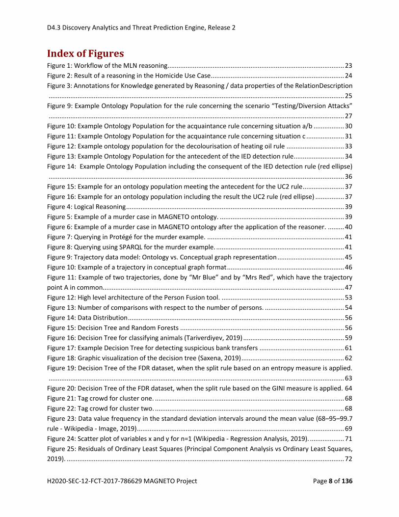
2.1.3.2 Communication and Social Relations
A rule has been suggested by The Police Academy in Szczytno (WSPol) to create a social relation between
persons that had telephone contact several times: If persons have contacted each other more than once
by telephone, it means that they can know their identity.
When creating a rule, the appropriate relations concerning a telephone call are:
hasTelephoneCaller: connects the event “TelephoneCall” to the person initiating the call
hasTelephoneCallee: connects the event “TelephoneCall” to the person receiving the call
Using this relations, there are three different situations how two telephone contacts between a person A
and B can happen:
a. Person A calls Person B two times
b. Person B calls Person A two times
c. Person A calls Person B and Person B calls Person A
Situations a. and b. can be covered by the same rule:
Event(tc1), hasCategory(tc), TelephoneCall(tc), hasTeleponeCallee(tc1, p1), hasTelephoneCaller(tc1, p2),
Event(tc2), hasCategory(tc), hasTelephoneCallee(tc2, p1), hasTelephoneCaller(tc2, p2), tc1!=tc2
isAcquaintanceOf(p1,p2)
One rule is sufficient, because the free variables p1 and p2 may be assigned as follows:
Situation a: p1=B, p2=A
Situation b: p1=A, p2=B
D4.3 Discovery Analytics and Threat Prediction Engine, Release 2
H2020-SEC-12-FCT-2017-786629 MAGNETO Project Page 30 of 136
Figure 5: Example Ontology Population for the acquaintance rule concerning situation a/b
The rule for situation c.):
Event(tc1), hasCategory(tc), TelephoneCall(tc), hasTeleponeCallee(tc1, p1), hasTeleponeCaller(tc1, p2),
Event(tc2), hCategory(tc), hasTelephoneCallee(tc2, p2), hasTelephoneCaller(tc2, p1), tc1!=tc2
isAcquaintanceOf(p1,p2)

D4.3 Discovery Analytics and Threat Prediction Engine, Release 2
H2020-SEC-12-FCT-2017-786629 MAGNETO Project Page 31 of 136
Figure 6: Example Ontology Population for the acquaintance rule concerning situation c
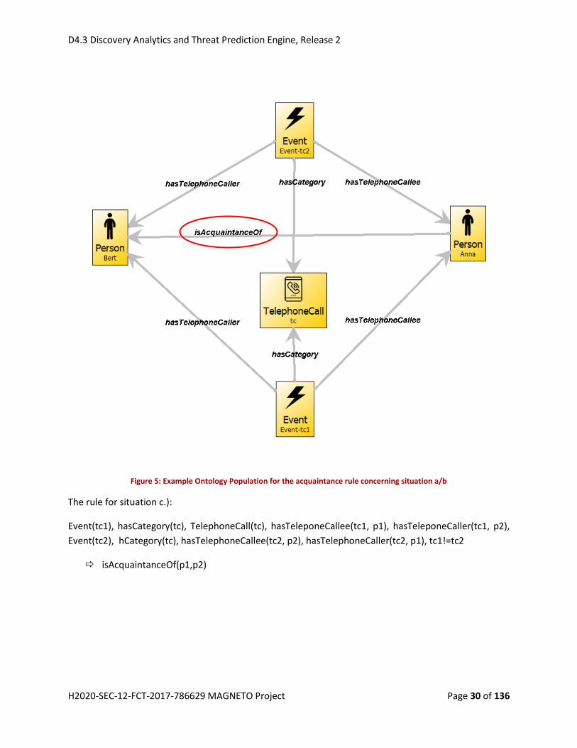
2.1.3.3 Use Case Fuel Crime - Decolourisation of Heating Oil
The Police Academy in Szczytno (WSPOL) has proposed a rule for the Use Case 4 concerning the fuel crime,
which is one of the main areas of activity of organised crime groups (OCG) and has the greatest impact on
the depletion of tax revenues. One of the modus operandi used by perpetrators most commonly is the
de-colourisation of heating oil. The company buys heating oil from Germany and resells it to other

D4.3 Discovery Analytics and Threat Prediction Engine, Release 2
H2020-SEC-12-FCT-2017-786629 MAGNETO Project Page 32 of 136
companies for heating purposes. The use of heating oil is a subject to a lower rate of excise duty in Poland.
Despite the declarations of going abroad, in fact, heating oil does not leave Poland, but is transported to
places where the oil is discolored (the removal of colorant). Then, this oil is delivered to petrol stations
and sold as a fuel, and so committing a tax fraud.
The following rule is proposed to detect illegal trade of heating oil:
If the owner of a petrol station has transferred money from his account to the account belonging to the
owner of the vehicle transporting the heating oil, the goods may have been used as fuel.
Missing concepts that have been added to the ontology:
FuelStation
TankLorry
Transport
FuelSmuggling
hasTransportLoad
BankAccount(bafs), FuelStation(fs), isBankAccountOf(bafs, fs), Person(pfs), hasOwnershipOf(pfs,fs)
Event(tra), hasCatgeory(tra, mtrans), MoneyTransaction(mtrans), hasOrderingPartyAccount (tra, bafs)
hasRecipientAccount (tra, batr), BankAccount(batr), Person(tro), isBankAccountOf(batr, tro),
TankLorry(tl), hasOwnershipOf(tro,tl), Transport(tp), Event(tpe), hasCategory(tpe, tp),
involvesObject(tpe, tl), hasTransportLoad(tpe,ho), HeatingOil(ho), FuelSmuggling(fs)
hasCrimeCategory(tpe, fs)
hasCrimeCategory(tra, fs)
isSuspect(tro, tpe)
isSuspect(tra, tra)
D4.3 Discovery Analytics and Threat Prediction Engine, Release 2
H2020-SEC-12-FCT-2017-786629 MAGNETO Project Page 33 of 136
Figure 7: Example ontology population for the decolourisation of heating oil rule
2.1.3.4 Use Case Planned IED-Attack from Electronic Devices based information
Concerning the use case of planned terroristic bombing attacks, the Police Service of Northern Ireland
(PSNI) has contributed facts that indicate suspicious persons, i.e. persons that have used an electronic
device (such as computer or mobile phone) for suspicious internet searches or the purchase of
components that might be used to construct improvised explosive devices:
a. Component parts used to make the improvised explosive device (IED)
b. Persons electronic devices shows searches on bomb making
c. Persons electronic device shows purchase of component parts of IED
These facts can be summarized in the following rule formulated in natural language:
If a person has used an electronic device to perform internet searches on bomb making and/or shows
purchases of component parts on their electronic device then the person is a suspect.
The implementation of this rule required some extensions of the ontology:

D4.3 Discovery Analytics and Threat Prediction Engine, Release 2
H2020-SEC-12-FCT-2017-786629 MAGNETO Project Page 34 of 136
A new concept class “SearchEngineSearchForTopic”, derived from EventCategory, has been
introduced as a child of concept “SearchingForInformation”, because the existing categories
supported the search for persons, events and objects only.
The event lacked a relation (object property) to link a search topic to the event, so a new object
property “involvesTopic” has been introduced, the range is very general
(“magnetoModelObject”).
Concerning internet search the existing concepts “SearchEngineSearchForObject” and
“SearchEngineSearchForPerson” have been complemented by “SearchEngineSearchForTopic”.
For describing the search topic, a new concept “ConstructionOfBombs” has been added as a child
of “IllegalManufacturingOfWeapons” in the section of “Crime_PotentialCrime”.
For simplifying the rule of the purchase of IED components, a new concept “IED_Chemicals” has
been added and the existing chemicals (Fertilizer, Hexamine, MEKP and Peroxide) have been
added as children to it.
As the ontology has no concept “ElectronicDevice”, but instead the concepts “Computer” and
“MobilePhone”, the rule has been formulated including both concepts connected by the boolean or-
operator (symbol “v” in the formula).
Figure 8: Example Ontology Population for the antecedent of the IED detection rule

D4.3 Discovery Analytics and Threat Prediction Engine, Release 2
H2020-SEC-12-FCT-2017-786629 MAGNETO Project Page 35 of 136
The natural language rule that has been suggested by the LEA has the connecting words “and/or” between
two different conditions. So, in fact these are two possibilities of creating the rule set:
1. When applying the “or”, then one of the two conditions is enough to make a person suspicious:
In this case we would have two rules having the same consequent, one for each condition:
Rule 1: Equipment(eq), (MobilePhone(ed) v Computer(ed)), isObjectInEquipment(ed, eq),
Person(p), hasOwnershipOf(p, ed), SearchEngineSearchForTopic(ses), Event(e), hasCategory(e,
ses), involvesTopic(cob), isEquipmentInEvent(eq, e), ConstructionOfBombs(cob) ), Bombing(bo)
=> isSuspectTerrorism(p, bo)
Rule 2: Purchase(pur), Event(ep), hasCategory(ep, pur), Person(p), involvesActingPerson(ep, p),
IED_Chemicals (iedc), involvesObject(e, iedc), Bombing(bo) => isSuspectTerrorism(p, bo)
2. When applying the “and”, both conditions have to be fulfilled, so we would have only one longer
rule:
Equipment(eq), (MobilePhone(ed) v Computer(ed)), isObjectInEquipment(ed, eq),
hasOwnershipOf(p, ed), SearchEngineSearchForTopic(ses), Event(e), hasCategory(e, ses),
involvesTopic(cob), ConstructionOfBombs(cob), isEquipmentInEvent(eq, e),
Purchase(pur), Event(ep), hasCategory(ep, pur), Person(p), involvesActingPerson(ep, p),
IED_Chemicals (iedc), involvesObject(e, iedc), Bombing(bo) => isSuspectTerrorism(p, bo)

D4.3 Discovery Analytics and Threat Prediction Engine, Release 2
H2020-SEC-12-FCT-2017-786629 MAGNETO Project Page 36 of 136
Figure 9: Example Ontology Population including the consequent of the IED detection rule (red ellipse)
2.1.3.5 Economic Organized Crime
From Use Case 2 described in (MINT, 2018), the following incident has been chosen for a rule: An
employee of a bank help to set up a bank account for a company that is suspected to be involved in an
organized crime, by accepting a forged identification document as proof of ID.
The following extensions to the ontology have been made:
AccountOpening: New concept class derived from EventCategory
IdCardVerification: New concept class derived from EventCategory
ForgedDocument, ForgedIdentityDocument: New concept class derived from ArtificialObjects

D4.3 Discovery Analytics and Threat Prediction Engine, Release 2
H2020-SEC-12-FCT-2017-786629 MAGNETO Project Page 37 of 136
Figure 10: Example for an ontology population meeting the antecedent for the UC2 rule
Event(bao), hasContext(bao, oe), OrganizedCrime(oe), isOrganisationInvolvedInEvent(co, bao),
Company(co), AccountOpening(ao), hasCategory(bao, ao), BankAccount(ba), involvesObject(bao, ba),
isBankAccountOf(ba, co), Bank(bnk), hasKeepingBank(ba, bnk),
Event(acc), isRelatedTo(bao, acc), hasCategory(acc,icv), IdCardVerification(icv), involvesActingPerson(acc,
emp), Person(emp), isMemberOf(emp, bnk), involvesObject(fid), ForgedIdentityDocument(fid)
=> isSuspectFraud(emp, bao)
Figure 11: Example for an ontology population including the result the UC2 rule (red ellipse)

D4.3 Discovery Analytics and Threat Prediction Engine, Release 2
H2020-SEC-12-FCT-2017-786629 MAGNETO Project Page 38 of 136
2.1.4 Logical Reasoning
2.1.4.1 Rules for logical reasoning
In our logical reasoning tool the SWRL (SWRL: A Semantic Web Rule Language Combining OWL and
RuleML, 2019) has been used in order to express the necessary rules that will allow the reasoner to infer
the new axioms (see section 2.1.1 for a general description of rules).One main advantage of SWRL is its
“human readable” form, in which both antecedent and consequent are conjunctions of atoms, written
𝑎1 ∧ 𝑎2 ∧ 𝑎3…∧ 𝑎𝑛 and the variables are indicated using the standard convention of prefixing them with
a question mark (e.g. ?x).
An atom or predicate is of the form C(x), P(x,y) or builtIn(r,x,...) where C is an OWL description (concept)
or data range, P is an OWL property or relation, r is a built-in relation, x and y are either variables, OWL
individuals or OWL data values, as appropriate.
Using this syntax, a rule asserting that the composition of parent and brother properties implies the
“uncle” property would be written:
𝑝𝑎𝑟𝑒𝑛𝑡(? 𝑥, ? 𝑦) ∧ 𝑏𝑟𝑜𝑡ℎ𝑒𝑟(? 𝑦, ? 𝑧) ⇒ 𝑢𝑛𝑐𝑙𝑒(? 𝑥, ? 𝑧)
These rules will be employed by the reasoner in order to infer new knowledge and uncover facts that have
not been initially asserted in the ontology. In this light, a set of rules has been developed for MAGNETO
and the work is ongoing. The rules that have been developed so far for the logical reasoning belong to the
below general categories:
Family Relationship Rules
General Relationship Rules
Criminality Rules
2.1.4.2 Reasoning
For the reasoning process the Pellet (Pellet: An Open Source OWL DL reasoner for Java, 2019) reasoner
has been employed, which can support the SWRL rules. It has been published under the AGPL v3 license
and it is a free open-source Java-based reasoner for OWL 2 and Semantic Web Rule Language. Pellet uses
a tableau-based decision procedure to provide many reasoning services (e.g. subsumption, satisfiability,
classification, instance retrieval, conjunctive query answering) along with the capability to generate
explanations for the inferences it computes. It has bindings for both OWL API and Jena libraries, and
supports the Protégé tool, command line and OWL API too. It supports reasoning services such as
realization, classification, satisfiability, conjunctive query answering, entailment, consistency and
explanation.
In order to allow the reasoner to infer the new axioms the following APIs have been used:
OWL API (The OWL API, 2019): It is a standard Java library and API for working with OWL ontologies (OWL
API main repository, 2019). It provides a standard interface to OWL reasoners, so different reasoners can
be used without any update in the implementation.

D4.3 Discovery Analytics and Threat Prediction Engine, Release 2
H2020-SEC-12-FCT-2017-786629 MAGNETO Project Page 39 of 136
SWRL API (Java API for working with the SWRL rule and SQWRL query languages, 2019): The SWRLAPI
(M.J. O'Connor, 2008) is a Java API for working with the OWL-based SWRL rule and SQWRL query
languages. It provides a collection of software components and Java-based APIs that allows among other
to create, edit and manage the SWRL rules.
The above APIs provide the appropriate tools to create a Pellet Reasoner and apply the SWRL rules in
order to infer the new knowledge in MAGNETO.
2.1.4.3 Approach
A simple flow of the reasoning procedure as described above is presented in Figure 12.
Figure 12: Logical Reasoning
In this paragraph, we present a simple example of the Logical Reasoner. Specifically, assume a simple rule
that a person is suspect for a murder event if the person is an enemy of the victim. This rule can be
described using SWRL as follows:
𝐸𝑣𝑒𝑛𝑡(? 𝑧)⋀𝑖𝑠𝐸𝑛𝑒𝑚𝑦𝑂𝑓(? 𝑥, ? 𝑦)⋀𝑖𝑠𝐷𝑒𝑎𝑑(? 𝑦, 𝑡𝑟𝑢𝑒)⋀𝑖𝑛𝑣𝑜𝑙𝑣𝑒𝑠𝑃𝑒𝑟𝑠𝑜𝑛(? 𝑧, ? 𝑦) ⇒ 𝑖𝑠𝑆𝑢𝑠𝑝𝑒𝑐𝑡(? 𝑥, ? 𝑧)
In this simple example, assume that person Dieter is enemy of Karl who has been murdered (Figure 13).
Figure 13: Example of a murder case in MAGNETO ontology.

D4.3 Discovery Analytics and Threat Prediction Engine, Release 2
H2020-SEC-12-FCT-2017-786629 MAGNETO Project Page 40 of 136
Using the reasoner with the above simple rule, we can infer the suspect of the case, as it can be seen in
the following result.
person : Dieter
inferred class for Dieter: magnetoModelObject
asserted class for Dieter: Person
inferred object property for Dieter: isSuspect -> MurderCase_3573
inferred object property for Dieter: involvesEntity -> MurderCase_3573
inferred object property for Dieter: socialRelation -> Karl
asserted object property for Dieter: isEnemyOf -> Karl
inferred object property for Dieter: involvesPerson -> MurderCase_3573
inferred object property for Dieter: hasEventObjectProperty -> MurderCase_3573
inferred object property for Dieter: hasPersonObjectProperty -> Karl
Is Dieter suspect for MurderCase_3573 ? : true
Then by adding the inferred axioms in the ontology the new relationships can be used (Figure 14) in order
to query the ontology and find all the necessary information.
Figure 14: Example of a murder case in MAGNETO ontology after the application of the reasoner.
Thus, we can query the results using the DL query in Protégé in order to find the suspect or by using
SPARQL. It is expected that for the purposes of MAGNETO the SPARQL will be used by the tools that LEAs
will interact with. These examples are depicted in Figure 15 and in Figure 16, respectively.

D4.3 Discovery Analytics and Threat Prediction Engine, Release 2
H2020-SEC-12-FCT-2017-786629 MAGNETO Project Page 41 of 136
Figure 15: Querying in Protégé for the murder example.
Figure 16: Querying using SPARQL for the murder example.
2.2 Graph Based Semantic Information Fusion Workflow The graph based semantic information fusion as introduced in deliverable D4.1 (ICCS, IOSB, QMUL, SIV,
TRT, 2019) is being developed with the intent of being a support to LEAs’ work. This section details the
implementation of the fusion tool, the data and processing workflow and shows how the final user
interacts with it.
Many types of data available to the LEAs include time and place information. When several such pieces of
information are related to a single object or person, they can define a trajectory. Such a trajectory consists
of a series of trajectory points and each trajectory point is defined by a time and a physical location. This
section details how to extract trajectories from various data sources and then process them to extract
relevant information for LEAs.

D4.3 Discovery Analytics and Threat Prediction Engine, Release 2
H2020-SEC-12-FCT-2017-786629 MAGNETO Project Page 42 of 136
Within the MAGNETO project, various LEAs contribute by providing anonymised datasets, which may be
also artificially generated. The datasets provide partial examples of typical information available within
an investigation, such as phone records, vehicle toll logs and written event descriptions. Furthermore,
various tools developed within the MAGNETO platform, such as feature recognition on CCTVs, could also
recover trajectory information on a relevant subject for LEAs.
2.2.1 Trajectory Extraction from Data Files
In order to be able to process generic data, the data importing tool needs to ignore any information which
does not fit in the MAGNETO model of trajectories defined in the MAGNETO ontology, first introduced in
the deliverable D4.1 (ICCS, IOSB, QMUL, SIV, TRT, 2019). This implies that as the tool parses the data being
imported, it will identify trajectories and ignore for this purpose the information that does not fit within
this model. This is motivated by the end-user requirement of minimizing false positives in the MAGNETO
platform: it is safer to ignore a piece of information rather than to risk having misleading information in
the context of a law enforcement investigation.
A more detailed and adapted data analysis would permit faithful extraction of this information, which the
tool may need to ignore, but this will have to be left to a future development (not in the scope of
MAGNETO) which is more closely calibrated to specific datasets.
In practice, these requirements mean that:
- Since a trajectory consists of at least two trajectory points having specified a place and a time as
introduced in deliverable D4.1 (ICCS, IOSB, QMUL, SIV, TRT, 2019), we only consider in the data
the combination of entries, which contain at least two pairs of different identifiable times and
places for a single object.
- If there is only one time and place information related to an object, this represents an event but
not yet a trajectory.
- If for a single entry there is extra information such as one time but two places, without further
information the tool needs to ignore the second position which does not have its own timestamp.
- If a data entry gives incomplete information, where part of the required information is not
identified for whatever reason (such as a name of place, which is not identified), the entry needs
to be ignored.
- If an entry gives redundant information from a previous accepted entry, it needs to be ignored,
possibly giving a warning if information is contradictory.
In the dataset example introduced in Table 3, containing vehicle toll data from Poland, each passage of a
vehicle is marked by a time “Data I czas”, a number plate “Numer rejestracyjny” identifying a car, and two
GPS coordinates which indicate a path on a section of road. A vehicle represented by a number plate can
have several passages in different places and times. In order to identify a trajectory, at least two distinct
trajectory points represented by a time and place pair are required.
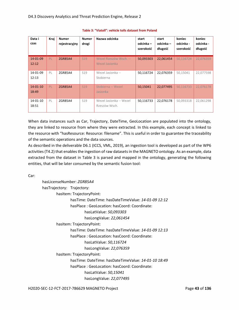
D4.3 Discovery Analytics and Threat Prediction Engine, Release 2
H2020-SEC-12-FCT-2017-786629 MAGNETO Project Page 43 of 136
Table 3: “Viatoll”: vehicle tolls dataset from Poland
Data i
czas
Kraj Numer
rejestracyjny
Numer
drogi
Nazwa odcinka start
odcinka –
szerokość
start
odcinka –
długość
koniec
odcinka -
szerokość
koniec
odcinka -
długość
14-01-09
12:12
PL ZGR85A4 S19 Wezel Rzeszów Wsch. --
Wezel Jasionka
50,093303 22,061454 50,116724 22,076359
14-01-09
12:13
PL ZGR85A4 S19 Wezel Jasionka --
Stobierna
50,116724 22,076359 50,15041 22,077598
14-01-10
18:49
PL ZGR85A4 S19 Stobierna -- Wezel
Jasionka
50,15041 22,077495 50,116733 22,076178
14-01-10
18:51
PL ZGR85A4 S19 Wezel Jasionka -- Wezel
Rzeszów Wsch.
50,116733 22,076178 50,093318 22,061298
When data instances such as Car, Trajectory, DateTime, GeoLocation are populated into the ontology,
they are linked to resource from where they were extracted. In this example, each concept is linked to
the resource with “hasResource: Resource: filename”. This is useful in order to guarantee the traceability
of the semantic operations and the data sources.
As described in the deliverable D6.1 (ICCS, VML, 2019), an ingestion tool is developed as part of the WP6
activities (T4.2) that enables the ingestion of raw datasets in the MAGNETO ontology. As an example, data
extracted from the dataset in Table 3 is parsed and mapped in the ontology, generating the following
entities, that will be later consumed by the semantic fusion tool:
Car:
hasLicenseNumber: ZGR85A4
hasTrajectory: Trajectory:
hasItem: TrajectoryPoint:
hasTime: DateTime: hasDateTimeValue: 14-01-09 12:12
hasPlace : GeoLocation: hasCoord: Coordinate:
hasLatValue: 50,093303
hasLongValue: 22,061454
hasItem: TrajectoryPoint:
hasTime: DateTime: hasDateTimeValue: 14-01-09 12:13
hasPlace : GeoLocation: hasCoord: Coordinate:
hasLatValue: 50,116724
hasLongValue: 22,076359
hasItem: TrajectoryPoint:
hasTime: DateTime: hasDateTimeValue: 14-01-10 18:49
hasPlace : GeoLocation: hasCoord: Coordinate:
hasLatValue: 50,15041
hasLongValue: 22,077495

D4.3 Discovery Analytics and Threat Prediction Engine, Release 2
H2020-SEC-12-FCT-2017-786629 MAGNETO Project Page 44 of 136
hasItem: TrajectoryPoint:
hasTime: DateTime: hasDateTimeValue: 14-01-10 18:51
hasPlace : GeoLocation: hasCoord: Coordinate:
hasLatValue: 50,116733
hasLongValue: 22,076178
Table 4 introduces an example of a telephone record dataset supplied by LEAs. The field “Data
rozpoczęcia” gives the time of a call, “Strona inicjująca” gives the telephone number of the source, which
identifies a device, and “Dane lokalizacyjne (długość; szerokość)” indicates the position of the antenna
relay from which this call was passed.
Table 4: Telephone record dataset
49990117334 - Wykaz połączeń za okres od 2014-05-25 do 2014-06-10.
Typ
połączen
ia
Data
rozpoczęc
ia
Strona
inicjująca
Strona
odbierająca
Wybiera
ne cyfry
Czas
trwania
połączen
ia
Numer
Imei
inicjujący
Numer
Imei
odbierają
cy
Dane lokalizacyjne
(długość;
szerokość)
W 25/05/20
14 06:03
499901173
34
4,88309E+
12
7999640
94
3 3,16379E+
14
21,473399;52,129
999
W 25/05/20
14 19:14
499901173
34
499841983
88
8419838
8
0 3,16379E+
14
21,488099;52,191
599
Similar to the previous example, the raw data from the telephone record dataset in Table 4 is ingested
into the ontology, following the format:
TelephoneNumber: 49990117334
hasTrajectory: Trajectory:
hasItem: TrajectoryPoint:
hasTime: DateTime: hasDateTimeValue: 25/05/2014 06:03
hasPlace : GeoLocation: hasCoord: Coordinate:
hasLatValue: 52,129999
hasLongValue: 21,473399
hasItem: TrajectoryPoint:
hasTime: DateTime: hasDateTimeValue: 25/05/2014 19:14
hasPlace : GeoLocation: hasCoord: Coordinate:
hasLatValue: 52,191599
hasLongValue: 21,488099
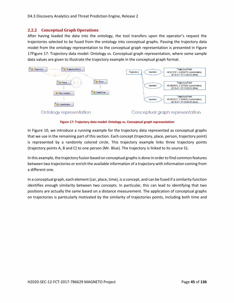
D4.3 Discovery Analytics and Threat Prediction Engine, Release 2
H2020-SEC-12-FCT-2017-786629 MAGNETO Project Page 45 of 136
2.2.2 Conceptual Graph Operations
After having loaded the data into the ontology, the tool transfers upon the operator’s request the
trajectories selected to be fused from the ontology into conceptual graphs. Passing the trajectory data
model from the ontology representation to the conceptual graph representation is presented in Figure
17Figure 17: Trajectory data model: Ontology vs. Conceptual graph representation, where some sample
data values are given to illustrate the trajectory example in the conceptual graph format.
Figure 17: Trajectory data model: Ontology vs. Conceptual graph representation
In Figure 10, we introduce a running example for the trajectory data represented as conceptual graphs
that we use in the remaining part of this section. Each concept (trajectory, place, person, trajectory point)
is represented by a randomly colored circle. This trajectory example links three trajectory points
(trajectory points A, B and C) to one person (Mr. Blue). The trajectory is linked to its source S1.
In this example, the trajectory fusion based on conceptual graphs is done in order to find common features
between two trajectories or enrich the available information of a trajectory with information coming from
a different one.
In a conceptual graph, each element (car, place, time), is a concept, and can be fused if a similarity function
identifies enough similarity between two concepts. In particular, this can lead to identifying that two
positions are actually the same based on a distance measurement. The application of conceptual graphs
on trajectories is particularly motivated by the similarity of trajectories points, including both time and
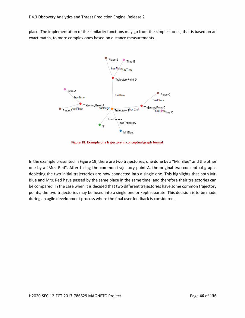
D4.3 Discovery Analytics and Threat Prediction Engine, Release 2
H2020-SEC-12-FCT-2017-786629 MAGNETO Project Page 46 of 136
place. The implementation of the similarity functions may go from the simplest ones, that is based on an
exact match, to more complex ones based on distance measurements.
In the example presented in Figure 19, there are two trajectories, one done by a “Mr. Blue” and the other
one by a “Mrs. Red”. After fusing the common trajectory point A, the original two conceptual graphs
depicting the two initial trajectories are now connected into a single one. This highlights that both Mr.
Blue and Mrs. Red have passed by the same place in the same time, and therefore their trajectories can
be compared. In the case when it is decided that two different trajectories have some common trajectory
points, the two trajectories may be fused into a single one or kept separate. This decision is to be made
during an agile development process where the final user feedback is considered.
Figure 18: Example of a trajectory in conceptual graph format

D4.3 Discovery Analytics and Threat Prediction Engine, Release 2
H2020-SEC-12-FCT-2017-786629 MAGNETO Project Page 47 of 136
Figure 19: Example of two trajectories, done by “Mr Blue” and by “Mrs Red”, which have the trajectory point A in common.
Once the trajectory fusion step is done, several types of requests may be done on top of the fused
information, serving various applications. Examples may include finding trajectories of a given person
using fused data from various sources, finding trajectories and people that have passed by a given place
and a given time, fusing trajectories for a given person and a given vehicle after it is identified that the
person was in the vehicle.
2.3 Machine Learning Based Person Fusion The Person Fusion Tool will be responsible for finding different person instances in the knowledge graph
that refer to the same person and fuse these instances. This high-level information fusion tool will
recognize the redundancy of the persons in the knowledge base and by fusing this information it will
increase the credibility of the MAGNETO system.
The Person Fusion Tool will check the similarities between the different person instances in the knowledge
base and calculate the probability of these different person-instances to refer to the same physical person.

D4.3 Discovery Analytics and Threat Prediction Engine, Release 2
H2020-SEC-12-FCT-2017-786629 MAGNETO Project Page 48 of 136
This will allow MAGNETO to deal with the uncertainty of person instances in the knowledge base.
Specifically, the Person Fusion Tool will check the persons in the knowledge base or new persons to enter
the knowledge base and if the new instance of the person refers to another person that already exists in
the database, it will calculate a degree of certainty that these persons need to be fused. However, the
decision of fusing these instances will be made at a higher-level by the end user of the MAGNETO system.
For this scope, the output of the module will be the instances of the persons along with a degree of belief
that these persons are required to be fused. After the end-user would confirm the decision in the
MAGNETO HMI, the module will fuse these instances.
2.3.1 Approach
As stated in D 4.1 (ICCS, IOSB, QMUL, SIV, TRT, 2019), the design of the Person Fusion Tool is based on a
variation of the k-Nearest Neighbour algorithm (K. Hechenbichler, 2004). Specifically, appropriate weights
have been applied to the contribution of each feature to the total similarity. The idea of weighting features
when using the k-NN technique is used to give more importance, in the classification process, to features
that are more relevant to the task. As a result, only a subset of the available features will be used to
determine if two persons in the instances are the same and should be fused. Assuming that a person 𝑝
can be characterized by 𝑛 features 𝑓(𝑖), 𝑖 = 1,…𝑛, then the similarity of two persons 𝑝𝑖 and 𝑝𝑗 can be
expressed as
𝑆𝑖𝑚𝑖𝑙𝑎𝑟𝑖𝑡𝑦(𝑝𝑖 , 𝑝𝑗) = ∑𝑤𝑘 × 𝑠𝑖𝑚𝑖𝑙𝑎𝑟𝑖𝑡𝑦(𝑓𝑖(𝑘), 𝑓𝑗(𝑘))
𝑛
𝑘=1
Where 𝑤𝑘 is the weight of feature 𝑘.
The selection of the appropriate initial values of the weights will be based on the domain knowledge of
the LEAs. However, the LEAs’ officers will be able to modify the weights appropriately after the
deployment of the system based on their specific needs.
2.3.2 Similarity
2.3.2.1 Numeric similarity
The numeric metrics, like the Euclidean distance and the Manhattan distance (Chomboon & al., 2015), are
very common in order to calculate the distance between two values. However, for the purposes of the
Person Fusion tool no numeric metrics have been used, and all numeric features have been treated as
text features. This approach is considered the most appropriate for features expected in MAGNETO in
order to cope with the typographical variations in data.
2.3.2.2 String based similarity
The string-based metrics are appropriate for symbolic/alphanumeric features. Some common metrics
include the:
Levenshtein distance. Levenshtein distance (Haldar & Mukhopadhyay, 2011) is a string metric for
measuring the similarity between two strings. In other words, the Levenshtein distance between
two strings is the number of single-character edits (insertions, deletions or substitutions) required

D4.3 Discovery Analytics and Threat Prediction Engine, Release 2
H2020-SEC-12-FCT-2017-786629 MAGNETO Project Page 49 of 136
to transform one word into the other. The greater the Levenshtein distance, the more different
the strings are. Mathematically, the Levenshtein distance between two strings s, t (of length
|𝑠|and |𝑡| respectively) is given by 𝑙𝑒𝑣𝑠,𝑡(|𝑠|, |𝑡|) where
𝑙𝑒𝑣𝑠,𝑡(𝑖, 𝑗) =
{
max
(𝑖, 𝑗) 𝑖𝑓 min(𝑖, 𝑗) = 0
𝑚𝑖𝑛 {
𝑙𝑒𝑣𝑠,𝑡(𝑖 − 1, 𝑗) + 1
𝑙𝑒𝑣𝑠,𝑡(𝑖, 𝑗 − 1) + 1
𝑙𝑒𝑣𝑠,𝑡(𝑖 − 1, 𝑗 − 1) + 1𝑠𝑖≠𝑡𝑗
𝑜𝑡ℎ𝑒𝑟𝑤𝑖𝑠𝑒
Where 1𝑠𝑖≠𝑡𝑗 is the indicator function equal to 0 when 𝑠𝑖 = 𝑡𝑗 and equal to 1 otherwise, and
𝑙𝑒𝑣𝑠,𝑡(𝑖, 𝑗) is the distance between the first 𝑖 characters of s and the first 𝑗 characters of t.
Jaro similarity. Jaro distance (Porter & Winkler, 1997) is another string metric for measuring
similarity between two strings. The Jaro similarity 𝑠𝑖𝑚𝑗 of two strings 𝑠1 and 𝑠2 is given by
𝑠𝑖𝑚𝑗 = {
01
3(𝑚
|𝑠1|+𝑚
|𝑠2|+𝑚 − 𝑡
𝑚)
Where |𝑠1| and |𝑠2| are the length of strings 𝑠1 and 𝑠2, respectively, m is the number of matching
characters and t is half the number of transpositions. In Jaro distance, two characters from strings
𝑠1 and 𝑠2 are considered matching only if they are the same and no further than ⌊max (|𝑠1|,|𝑠2|)
2⌋-1.
In contrast to the other distance metrics, the greater the Jaro distance of two strings is, the more
similar these strings are. In Jaro distance, the score is normalized such that 0 equates to no
similarity and 1 is a perfect match.
Jaro-Winkler similarity. The Jaro-Winkler similarity (Winkler, 1990) is an extension of Jaro
similarity, which uses a prefix scale 𝑝 that gives more favorable ratings to strings that match from
the beginning for a set prefix length 𝑙. The Jaro-Winkler similarity 𝑠𝑖𝑚𝑤 of two strings 𝑠1 and 𝑠2 is
given by
𝑠𝑖𝑚𝑤 = 𝑠𝑖𝑚𝑗 + 𝑙 ∙ 𝑝(1 − 𝑠𝑖𝑚𝑗)
Where 𝑠𝑖𝑚𝑗 is the Jaro similarity of strings 𝑠1 and 𝑠2, 𝑙 is the length of the common prefix at the
start of the string and up to a maximum of four characters, and 𝑝 is a constant scaling factor for
how much the score is adjusted upwards for having common prefixes. 𝑝 should not exceed 0.25,
otherwise the similarity could become larger than 1. The standard value for this constant in
Winkler's work is 𝑝 = 0.1
In order to evaluate the performance of the above metrics, a set of surnames has been created (Keen,
2019). The above metrics have been used in order to calculate the similarity between the surnames. The
results are depicted in Table 5. From these results, it becomes obvious that the Jaro-Winkler outperforms
the other two metrics with respect to the processing time. For the purposes of the Person Fusion Tool the
Jaro-Winkler similarity has been used.

D4.3 Discovery Analytics and Threat Prediction Engine, Release 2
H2020-SEC-12-FCT-2017-786629 MAGNETO Project Page 50 of 136
Table 5: Comparison results between algorithms for string-based similarity.
Number of
Surnames
Number of
comparisons
Levenshtein
(calculation time
in seconds)
Jaro
(calculation time
in seconds)
Jaro-Winkler
(calculation time in
seconds)
1000 4.995 × 10⁵ 2.427539 2.340737 2.315805
10000 4.9995 × 10⁷ 5.642909 3.566460 3.392924
100000 4.9995 × 10⁹ 307.759326 85.334826 81.739669
2.3.2.3 Phonetic based similarity
The above metrics that have been presented focus on the string-based representation of the features.
However, string may be phonetically similar even if they are not similar in a character level (A. Elmagarmid,
2007). Some common algorithms for phonetic similarity include:
Soundex. The Soundex (The Soundex Indexing System, 2019) which was invented by Russell is
considered as the most common phonetic coding scheme. Soundex is based on the assignment of
identical code digits to phonetically similar groups of consonants and is used mainly to match
surnames. In the work of Newcombe it is reported that the Soundex code remains largely
unchanged, exposing about two-thirds of the spelling variations observed in linked pairs of vital
records, and that it sets aside only a small part of the total discriminating power of the full
alphabetic surname. Though, Soundex though designed primarily for Caucasian surnames, it
works pretty well for names of many different origins. However, when the names are of
predominantly East Asian origin, this code is less satisfactory because much of the discriminating
power of these names resides in the vowel sounds, which the code ignores.
New York State Identification and Intelligence System. The NYSIIS (Taft, Feb 1970) system was
proposed by Taft, and it differs from the Soundex in that it retains information about the position
of vowels in the encoded word by converting most vowels to the letter A. Furthermore, NYSIIS in
contrast to the Soundex, does not use numbers to replace letters; instead, it replaces consonants
with other phonetically similar letters, thus returning a pure alpha code (no numeric component).
Usually, the NYSIIS code for a surname is based on a maximum of nine letters of the full
alphabetical name, and the NYSIIS code itself is then limited to six characters. Taft in his work
(Taft, Feb 1970) compared Soundex with NYSIIS, using a name database of New York State, and
concluded that NYSIIS is 98.72 percent accurate, while Soundex is 95.99 percent accurate for
locating surnames. The NYSIIS encoding system is used today by the New York State Division of
Criminal Justice Services. The NYSIIS algorithm is presented below.
1. If the first letters of the name are
'MAC' then change these letters to 'MCC'
'KN' then change these letters to 'NN'
'K' then change this letter to 'C'
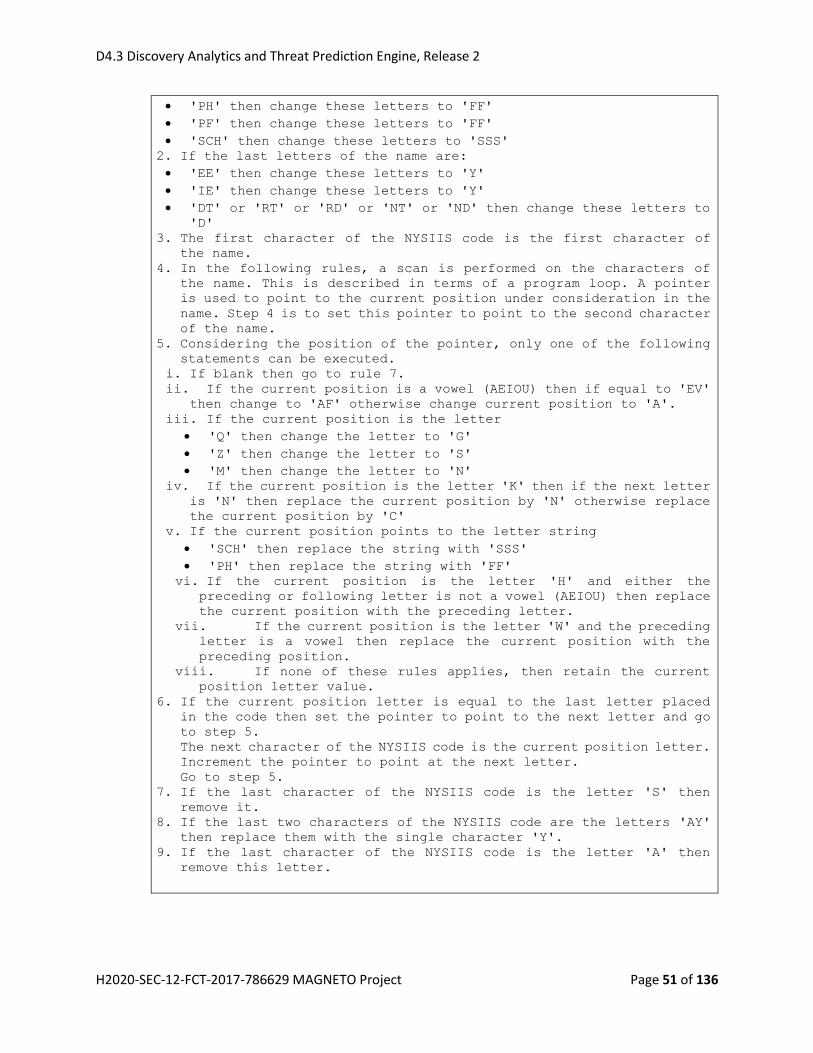
D4.3 Discovery Analytics and Threat Prediction Engine, Release 2
H2020-SEC-12-FCT-2017-786629 MAGNETO Project Page 51 of 136
'PH' then change these letters to 'FF'
'PF' then change these letters to 'FF'
'SCH' then change these letters to 'SSS'
2. If the last letters of the name are:
'EE' then change these letters to 'Y'
'IE' then change these letters to 'Y'
'DT' or 'RT' or 'RD' or 'NT' or 'ND' then change these letters to
'D'
3. The first character of the NYSIIS code is the first character of the name.
4. In the following rules, a scan is performed on the characters of the name. This is described in terms of a program loop. A pointer
is used to point to the current position under consideration in the
name. Step 4 is to set this pointer to point to the second character
of the name.
5. Considering the position of the pointer, only one of the following statements can be executed.
i. If blank then go to rule 7. ii. If the current position is a vowel (AEIOU) then if equal to 'EV'
then change to 'AF' otherwise change current position to 'A'.
iii. If the current position is the letter
'Q' then change the letter to 'G'
'Z' then change the letter to 'S'
'M' then change the letter to 'N'
iv. If the current position is the letter 'K' then if the next letter
is 'N' then replace the current position by 'N' otherwise replace
the current position by 'C'
v. If the current position points to the letter string
'SCH' then replace the string with 'SSS'
'PH' then replace the string with 'FF'
vi. If the current position is the letter 'H' and either the
preceding or following letter is not a vowel (AEIOU) then replace
the current position with the preceding letter.
vii. If the current position is the letter 'W' and the preceding
letter is a vowel then replace the current position with the
preceding position.
viii. If none of these rules applies, then retain the current
position letter value.
6. If the current position letter is equal to the last letter placed in the code then set the pointer to point to the next letter and go
to step 5.
The next character of the NYSIIS code is the current position letter.
Increment the pointer to point at the next letter.
Go to step 5.
7. If the last character of the NYSIIS code is the letter 'S' then remove it.
8. If the last two characters of the NYSIIS code are the letters 'AY' then replace them with the single character 'Y'.
9. If the last character of the NYSIIS code is the letter 'A' then remove this letter.

D4.3 Discovery Analytics and Threat Prediction Engine, Release 2
H2020-SEC-12-FCT-2017-786629 MAGNETO Project Page 52 of 136
Metaphone and Double Metaphone. Metaphone (Philips, Hanging on the Metaphone, 1990) and
Double Metaphone (Philips, The Double Metaphone Search Algorithm, 2000) are algorithms
suggested as better alternatives to Soundex by Philips. Specifically, in Metaphone 16 consonants
sounds are used in order to describe a large number of sounds used in many English and non-
English words. Double Metaphone which is a better version of Metaphone, allows multiple
encodings for names that have various possible pronunciations. The introduction of multiple
phonetic encodings greatly enhances the matching performance with rather a small overhead.
Specifically, Double Metaphone returns both a primary and a secondary code for a string which
accounts for some ambiguous cases as well as for multiple variants of surnames with common
ancestry. For example, encoding the name "Smith" yields a primary code of SM0 and a secondary
code of XMT, while the name "Schmidt" yields a primary code of XMT and a secondary code of
SMT—both have XMT in common. Double Metaphone tries to account for myriad irregularities in
English of Slavic, Germanic, Celtic, Greek, French, Italian, Spanish, Chinese, and other origin, by
using a much more complex ruleset for coding than Metaphone.
The results of the encoding of some common European surnames (Wikipedia, 2019) using the above
schemes are presented in Table 6. In order to find the similarity between the surnames, a string-based
metric (Jaro-Winkler) will be applied to the encoded results of the phonetic scheme.
Table 6: Phonetic encoding of common European surnames.
Surname Soundex Double Metaphone
NYSIIS
Silva S410 SLF, - SALV
Smith S530 SM0, XMT SNATH
Martin M635 MRTN, - MARTAN
Gruber G616 KRPR, - GRABAR
Huber H160 HPR, - HABAR
Hasanov H251 HSNF, - HASANAV
Georgiev G621 JRJF, KRKF GARGAF
Tamm T500 TM, - TAN
Korhonen K650 KRNN, - CARANAN
Beridze B632 PRTS, - BARADS
Schmidt S253 XMT, SMT SNAD
Rossi R200 RS, - RAS
Kazlauskas K242 KSLS, KTSL CASLASC
Borg B620 PRK, - BARG
Nowak N200 NK, - NAC
Smirnov S565 SMRN, XMRN SNARNAV

D4.3 Discovery Analytics and Threat Prediction Engine, Release 2
H2020-SEC-12-FCT-2017-786629 MAGNETO Project Page 53 of 136
2.3.3 Person Fusion Tool Architecture and Design Choices
The estimation whether two persons refer to the same instance and the respective degree of confidence
is based on both the numeric and the string-based features of the person. The high-level architecture of
the Person Fusion Tool is presented in Figure 20. The numeric features are compared between the person
instances by using the string-based similarity measures, and specifically the Jaro-Winkler similarity. On
the other hand, the string features are processed by examining both the character-based similarity and
the phonetic similarity. For the character-based similarity, the Jaro-Winkler similarity is employed, while
for the phonetic similarity, a hybrid approach has been adopted and the text is encoded using Double
Metaphone and the NYSIIS algorithm. Each of the encoded results undergoes a character-based
comparison in order to calculate the respective similarity and then the obtained results of the two
methods are weighted accordingly in order to estimate the phonetic similarity. Finally, the phonetic and
the character-based similarity of the string features are weighted again in order to estimate the overall
similarity of the feature.
Figure 20: High level architecture of the Person Fusion tool.
2.3.4 Improving the Efficiency of the Person Fusion Tool
In this paragraph, a discussion about the efficiency of the Person Fusion tool is provided. Specifically, the
Person Fusion tool should compare two person instances and conclude whether they refer to the same
person using a degree of belief. Assuming that there are 𝑁 persons in the system, then the Person Fusion
tool will require (𝑁2) comparisons for the first time and 𝑁 comparisons for any new person added in the
system or his/her information are updated.

D4.3 Discovery Analytics and Threat Prediction Engine, Release 2
H2020-SEC-12-FCT-2017-786629 MAGNETO Project Page 54 of 136
Figure 21: Number of comparisons with respect to the number of persons.
The initial comparisons may cause a high overhead in the system as can be seen in Figure 21, requiring
thus a more efficient approach. In this light, there are many techniques that can be applied in order to
improve the efficiency of the tool:
Early termination technique. In this technique (A. Elmagarmid, 2007), the comparison of two persons
terminates when they are concluded to be not equal after processing only a small portion of the
features of these two instances. With this technique only the basic features are processed and if they
do not match, then the comparison terminates concluding that the person instances are different
even if the rest of the features match exactly.
Blocking technique. In the blocking technique (A. Elmagarmid, 2007) the person instances are divided
in mutually exclusive subsets (blocks) with the assumption that all the person instances that refer to
the same person exist in the same block. These blocks will be created by using the appropriate
function (such as NYSIIS) on highly discriminating fields (such as surname) in order to group the
persons to the appropriate blocks. One of the main problems of this technique is that it may lead to
an increased number of false mismatches due to the failure of categorizing in the same group two
persons instances that though they are similar they do not agree on the blocking field. A possible
solution in this will be to execute the comparison phase multiple times using a different blocking field
each time.
Sorted neighborhood approach technique. In this technique (Hernandez & Stolfo, 1998), a key for each
person is computed by using the appropriate features (e.g. surname). Then, the persons are sorted in
a list and only those that are near each other are compared using a fixed size window. The window is
then moved through the sequential list and only the persons within the window are compared. This

D4.3 Discovery Analytics and Threat Prediction Engine, Release 2
H2020-SEC-12-FCT-2017-786629 MAGNETO Project Page 55 of 136
method is based on the assumption that person instances that refer to the same person will be close.
However, the effectiveness of this method depends on the selection of the key and, thus, it might not
compare persons that though they are similar they have different keys. A possible solution for this is
to execute multiple runs of this method with different keys and a small window each time.
For the purposes of MAGNETO, the early termination technique has been adopted for the Person Fusion
Tool.
2.4 Machine Learning Based Event Information Fusion Machine Learning Based Event Information Fusion will have as approach the following functionalities:
1. Classify or predict events using a cause-effect approach
2. The cause is composed by a set of entities and events registered as known ontology by the
MAGNETO components
3. The effect is a detected or predicted class of events
Event Information Fusion will have as inputs:
Quantitative or Qualitative representation of:
o Static Biometric Data o Online live biometric data o Static Text Data from databases, media o Online trigger event data collected from different sources including media and social
network o Attributes of entities and event
The outputs will be:
Classes of events considered as effects of matching patterns in input data
o Identified events or entities o Forecasted events
Processing Flow:
Preprocessing
o Normalization o Filtering o Lack of information treatment (filter or fill in)
Learning
o Dimensionality reduction (Nonlinear Kernel PCA) o Training (Classification And Regression Trees) o Testing and Validation
Application (Classification And Regression Trees)
o Classification o Regression
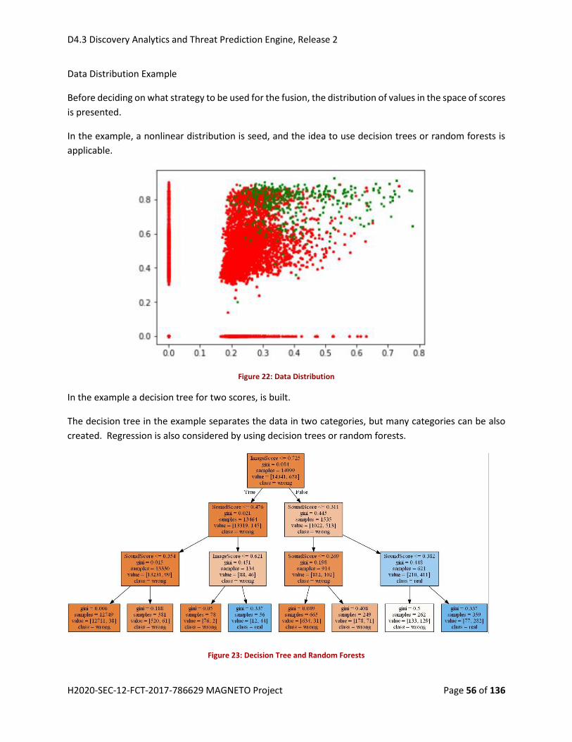
D4.3 Discovery Analytics and Threat Prediction Engine, Release 2
H2020-SEC-12-FCT-2017-786629 MAGNETO Project Page 56 of 136
Data Distribution Example
Before deciding on what strategy to be used for the fusion, the distribution of values in the space of scores
is presented.
In the example, a nonlinear distribution is seed, and the idea to use decision trees or random forests is
applicable.
Figure 22: Data Distribution
In the example a decision tree for two scores, is built.
The decision tree in the example separates the data in two categories, but many categories can be also
created. Regression is also considered by using decision trees or random forests.
Figure 23: Decision Tree and Random Forests

D4.3 Discovery Analytics and Threat Prediction Engine, Release 2
H2020-SEC-12-FCT-2017-786629 MAGNETO Project Page 57 of 136
The tools used to train the system and create the decision trees or random forests were based on Python
language, Python Jupyter and the Python libraries:
Pandas (to read data stored in csv files)
ScikitLearn (to train the system and get decision trees or random forests)
Tensorflow (for complex parallel machine learning processes)
Data visualization was based on Python Matplotlib library, with extension for saving data in png or jpg
format
Exposure to other systems, based on REST services was created using Python Flask library.
The rest APIs are the communication point for complex clients which are used to apply the decision based
on the decision trees created previously during the training process.
Processed data are exposed in the format of csv files or REST lists of objects for presentation in Graphana
visualization system.

D4.3 Discovery Analytics and Threat Prediction Engine, Release 2
H2020-SEC-12-FCT-2017-786629 MAGNETO Project Page 58 of 136
3. Advanced Correlation Engine
3.1 Classification of Datasets Based on Machine Learning
3.1.1 General Overview
In statistics and machine learning, classification is a supervised learning practise in which the system learns
from the supplied data input and later uses this learning to classify new data. This dataset may simply be
bi-class (i.e. whether the person is male or female) or it may be multi-class too. Some examples of
classification problems are bio-metric identification, document classification, classification of suspicious
transactions etc.
Here we have the types of classification algorithms in Machine Learning:
Linear Classifiers: Logistic Regression, Naive Bayes Classifier
Nearest Neighbour
Support Vector Machines
Decision Trees
Boosted Trees
Random Forest
Neural Networks
3.1.2 Decision Trees
The choice of a suitable algorithm has been taken with respect to the requirement of explainability that
is demanded from the ethical and legal perspective of the MAGNETO project. In the deliverable D9.1 (KUL,
CBRNE, 2019) section 6.2.2 “Explainability” is defined as “explaining of the workings of the system at both
the global level as well as in relation to particular cases and circumstances”. With respect to this demand,
the decision tree has been chosen because of its big advantage that the classifier generated is highly
interpretable.
A decision tree is a decision support tool that builds classification or regression models in the form of a
tree structure. It is used to assign a target value to an item that is given by a vector of observed values,
so-called indicator values. The vector of indicator values is often referred to as a dataset. The target value
is the class that the dataset is assigned to. Decision trees can handle both categorical and numerical data.
Essentially, the tool learns a hierarchy of “if-else” questions, leading to a decision. A decision tree is a
flowchart like tree structure, where each internal node denotes a test on an attribute, each branch
represents an outcome of the test, and each leaf node (terminal node) holds a class label.
The decision tree breaks down a dataset into smaller and smaller subsets while at the same time an
associated decision tree is incrementally developed. The final result is a tree with decision nodes and leaf
nodes. A decision node has two or more branches and a leaf node represents a classification or decision.
The topmost decision node in a tree that corresponds to the best predictor, is called root node.
(Sudhamathy & Venkateswaran, 2019).
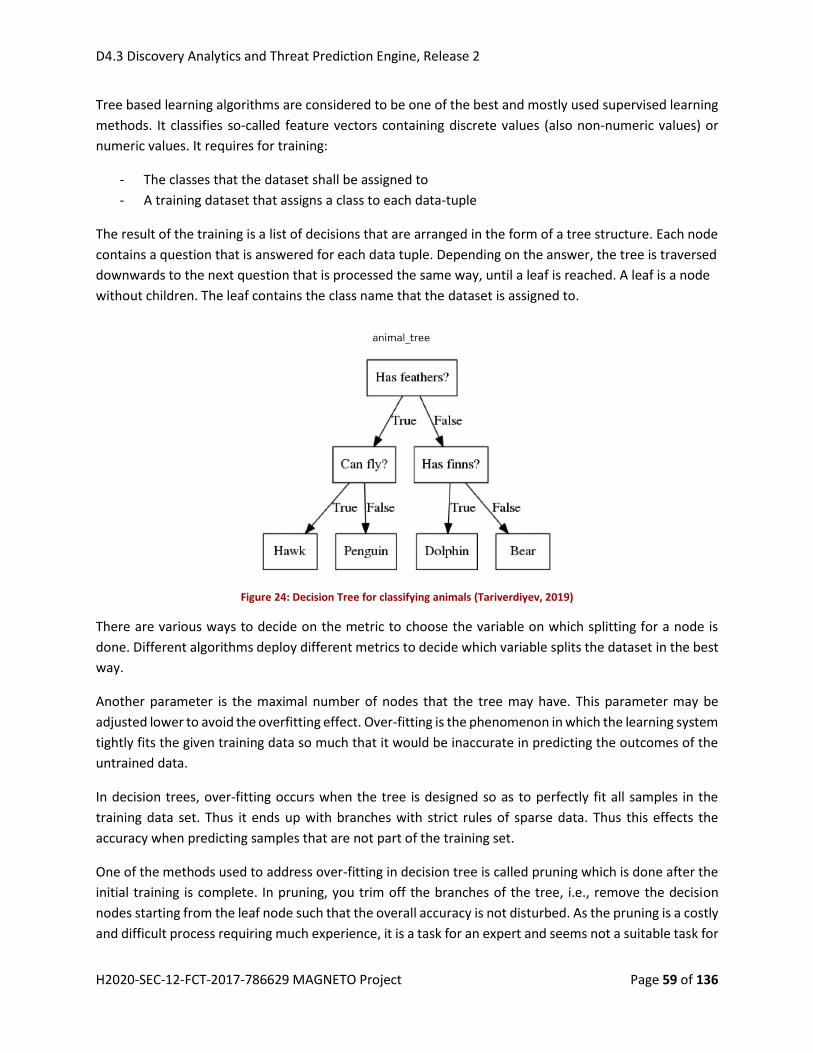
D4.3 Discovery Analytics and Threat Prediction Engine, Release 2
H2020-SEC-12-FCT-2017-786629 MAGNETO Project Page 59 of 136
Tree based learning algorithms are considered to be one of the best and mostly used supervised learning
methods. It classifies so-called feature vectors containing discrete values (also non-numeric values) or
numeric values. It requires for training:
- The classes that the dataset shall be assigned to
- A training dataset that assigns a class to each data-tuple
The result of the training is a list of decisions that are arranged in the form of a tree structure. Each node
contains a question that is answered for each data tuple. Depending on the answer, the tree is traversed
downwards to the next question that is processed the same way, until a leaf is reached. A leaf is a node
without children. The leaf contains the class name that the dataset is assigned to.
Figure 24: Decision Tree for classifying animals (Tariverdiyev, 2019)
There are various ways to decide on the metric to choose the variable on which splitting for a node is
done. Different algorithms deploy different metrics to decide which variable splits the dataset in the best
way.
Another parameter is the maximal number of nodes that the tree may have. This parameter may be
adjusted lower to avoid the overfitting effect. Over-fitting is the phenomenon in which the learning system
tightly fits the given training data so much that it would be inaccurate in predicting the outcomes of the
untrained data.
In decision trees, over-fitting occurs when the tree is designed so as to perfectly fit all samples in the
training data set. Thus it ends up with branches with strict rules of sparse data. Thus this effects the
accuracy when predicting samples that are not part of the training set.
One of the methods used to address over-fitting in decision tree is called pruning which is done after the
initial training is complete. In pruning, you trim off the branches of the tree, i.e., remove the decision
nodes starting from the leaf node such that the overall accuracy is not disturbed. As the pruning is a costly
and difficult process requiring much experience, it is a task for an expert and seems not a suitable task for

D4.3 Discovery Analytics and Threat Prediction Engine, Release 2
H2020-SEC-12-FCT-2017-786629 MAGNETO Project Page 60 of 136
the LEA enduser. So diminishing the number of nodes is the much less complicated option for addressing
the overfitting problem.
3.1.3 Application in MAGNETO
Classification of datasets may be applied to big datasets that shall be classified to structure the datasets
to categories that are predefined by the user. A possible classification might be the aspect if an event is
suspect or criminal. Such an event might be a bank transfer, a transport of goods, a car accident, etc. It is
important though, that the datasets describing the event contains enough indicator values that are
relevant for the desired classification. The indicator values might describe the properties of the event as
well as attributes of participating persons.
The appendix of deliverable D9.1 (KUL, CBRNE, 2019) specifies several requirements addressing the
avoidance of unfair bias in the tools and the training. Concerning R1.3 (“automated profiles provided by
the system must not contain discriminatory or unfair biases”), the tool will not be delivered with trained
decision trees, because the datasets lack the information of the classification, however no sensitive
attributes have been found in the datasets, so the R18.1 has been respected (“MAGNETO is being trained
with datasets devoid of sensitive attributes to mitigate discriminatory outcomes “). The training of the
decision trees will be done by the LEAs. As a result, the training datasets must be chosen carefully to avoid
a bias due to a not representative selection of datasets. Indicator values describing critical personal
attributes such as the affiliation to an ethnicity or sexual orientation should be avoided if possible to
prevent an ethical critical bias when training the classifier. The decision tree tool itself has no knowledge
of the semantics of the indicator values, the values are simply numbers or symbols to the tool. So the tool
cannot recognize or warn to avoid an ethical critical bias. The user that assembles the training sets must
be aware of it and has the obligation so carefully select the training datasets. Using bigger training datasets
may reduce the risk of unwanted bias.
The advantage of decision trees is given by the fact that a critical bias becomes very evident when checking
the visual graph of the decision tree. In that case, the choice of the training dataset can be revised to
remove the critical decision node from the tree, i.e. by removing the column containing the critical
attribute from the dataset

D4.3 Discovery Analytics and Threat Prediction Engine, Release 2
H2020-SEC-12-FCT-2017-786629 MAGNETO Project Page 61 of 136
Figure 25: Example Decision Tree for detecting suspicious bank transfers
3.1.4 Implementation
The tool is developed using the open-source2 software Smile (Statistical Machine Intelligence and Learning
Engine). Smile is a fast and comprehensive machine-learning engine with advanced data structures and
algorithms, supporting the development in Java or Scala language. It supports various input formats for
data: (Li, 2019)
Weka ARFF (attribute relation file format) is an ASCII text file format that is essentially a CSV file
with a header that describes the meta data. ARFF was developed for use in the Weka machine
learning software.
LibSVM is a very fast and popular library for support vector machines. LibSVM uses a sparse format
where zero values do not need to be stored. Each line of a libsvm file is in the format:
<label> <index1>:<value1> <index2>:<value2> ...
Delimited Text and CSV (Comma-separated values): Any character may be used to separate the
values, but the most common delimiters are the comma, tab, and colon.
other formats that are not relevant for the intended use in MAGNETO, mostly used by scientists:
MicroArray, Coordinate Triple Tuple List, Harwell-Boeing Column-Compressed Sparse Matrix and
Wireframe.
The output is the same data table with an additional column that contains the predicted target value (the
class it has been assigned to). Additionally it returns the graphic representation in Graphviz dot format.
Graphviz is an open-source graph visualization software representing structural information as diagrams
2 Licensed under the Apache License, Version 2.0
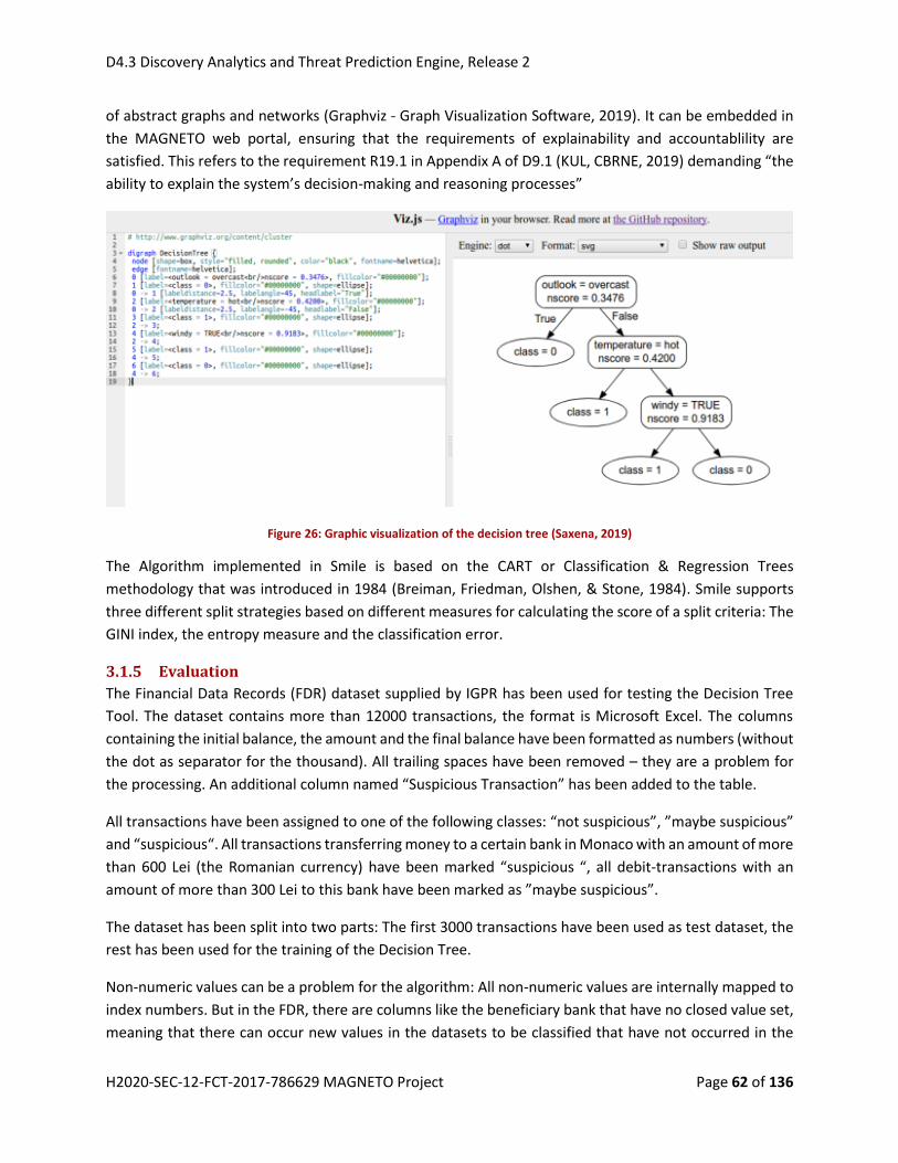
D4.3 Discovery Analytics and Threat Prediction Engine, Release 2
H2020-SEC-12-FCT-2017-786629 MAGNETO Project Page 62 of 136
of abstract graphs and networks (Graphviz - Graph Visualization Software, 2019). It can be embedded in
the MAGNETO web portal, ensuring that the requirements of explainability and accountablility are
satisfied. This refers to the requirement R19.1 in Appendix A of D9.1 (KUL, CBRNE, 2019) demanding “the
ability to explain the system’s decision-making and reasoning processes”
Figure 26: Graphic visualization of the decision tree (Saxena, 2019)
The Algorithm implemented in Smile is based on the CART or Classification & Regression Trees
methodology that was introduced in 1984 (Breiman, Friedman, Olshen, & Stone, 1984). Smile supports
three different split strategies based on different measures for calculating the score of a split criteria: The
GINI index, the entropy measure and the classification error.
3.1.5 Evaluation
The Financial Data Records (FDR) dataset supplied by IGPR has been used for testing the Decision Tree
Tool. The dataset contains more than 12000 transactions, the format is Microsoft Excel. The columns
containing the initial balance, the amount and the final balance have been formatted as numbers (without
the dot as separator for the thousand). All trailing spaces have been removed – they are a problem for
the processing. An additional column named “Suspicious Transaction” has been added to the table.
All transactions have been assigned to one of the following classes: “not suspicious”, ”maybe suspicious”
and “suspicious“. All transactions transferring money to a certain bank in Monaco with an amount of more
than 600 Lei (the Romanian currency) have been marked “suspicious “, all debit-transactions with an
amount of more than 300 Lei to this bank have been marked as ”maybe suspicious”.
The dataset has been split into two parts: The first 3000 transactions have been used as test dataset, the
rest has been used for the training of the Decision Tree.
Non-numeric values can be a problem for the algorithm: All non-numeric values are internally mapped to
index numbers. But in the FDR, there are columns like the beneficiary bank that have no closed value set,
meaning that there can occur new values in the datasets to be classified that have not occurred in the
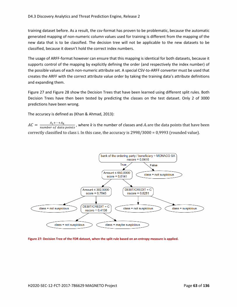
D4.3 Discovery Analytics and Threat Prediction Engine, Release 2
H2020-SEC-12-FCT-2017-786629 MAGNETO Project Page 63 of 136
training dataset before. As a result, the csv-format has proven to be problematic, because the automatic
generated mapping of non-numeric column values used for training is different from the mapping of the
new data that is to be classified. The decision tree will not be applicable to the new datasets to be
classified, because it doesn’t hold the correct index numbers.
The usage of ARFF-format however can ensure that this mapping is identical for both datasets, because it
supports control of the mapping by explicitly defining the order (and respectively the index number) of
the possible values of each non-numeric attribute set. A special CSV-to-ARFF converter must be used that
creates the ARFF with the correct attribute value order by taking the training data’s attribute definitions
and expanding them.
Figure 27 and Figure 28 show the Decision Trees that have been learned using different split rules. Both
Decision Trees have then been tested by predicting the classes on the test dataset. Only 2 of 3000
predictions have been wrong.
The accuracy is defined as (Khan & Ahmad, 2013):
𝐴𝐶 = 𝐴1+⋯+𝐴𝑘
𝑛𝑢𝑚𝑏𝑒𝑟 𝑜𝑓 𝑑𝑎𝑡𝑎 𝑝𝑜𝑖𝑛𝑡𝑠 , where k is the number of classes and Ai are the data points that have been
correctly classified to class i. In this case, the accuracy is 2998/3000 = 0,9993 (rounded value).
Figure 27: Decision Tree of the FDR dataset, when the split rule based on an entropy measure is applied.

D4.3 Discovery Analytics and Threat Prediction Engine, Release 2
H2020-SEC-12-FCT-2017-786629 MAGNETO Project Page 64 of 136
Figure 28: Decision Tree of the FDR dataset, when the split rule based on the GINI measure is applied.
3.2 Clustering Natural Language Text Documents
3.2.1 Motivation
Text clustering means to group together documents with similar content. Such a pre-processing step may
support subsequent text mining algorithms like (topic) classification, information retrieval and extraction
as well as document summarization.
E.g. search results in information retrieval may be grouped in different clusters to support the user in
navigating his search results. In information extraction tasks, it may be important to have related
documents together while extracting information artefacts, to get relations between the similar
documents efficiently. Related information is scattered over documents and it is advantageous for the
fusion algorithms to have these documents in one cluster. Another task may be to confirm certain
statements by analysing documents in that cluster.
Basic methods of clustering are connectivity-(hierarchical-), centroid-, distribution-, and density-based
clustering. There are almost 100 clustering algorithms, which fall in one of these categories. The different
clustering algorithms require certain sets of configuration parameters, which are external to the model;
the correct selection of these parameters is generally a difficult task as with most data mining techniques,
which are mainly explorative.
Machine learning algorithms e.g. clustering needs numerical vectors to compute the membership of a
data point to a cluster. This requires transforming text (documents, sentences, words) to numerical
vectors (i.e. the text model). There are certain approaches, the classic approach uses tf*idf (term
frequency, inverse document frequency (Rajaraman & Ullman, 2011)) score of term importance values to
build up the vector. Since 2013 there is a newer approach called word embedding (word2vec algorithm
(Mikolov, Chen, Corrado, & Dean, 2013)), which is mainly used with deep learning algorithms for text

D4.3 Discovery Analytics and Threat Prediction Engine, Release 2
H2020-SEC-12-FCT-2017-786629 MAGNETO Project Page 65 of 136
understanding, requiring massive volumes of training data from the LEA domain which is not available in
the required amount
For the implementation in MAGNETO, we use the tf*idf sentence encoding, the indices are stored in an
Apache LuceneTM index store. The sentence encoding allows the interpretation of a sentence as a
numerical data point in a high-dimensional vector space model. As the size of the vocabulary will have a
magnitude of 1000 or 10000, the vectors are sparse, which requires an efficient numerical handling of the
algorithms for sparse vectors and matrices, which incorporates only the subspaces (i.e. areas with values
greater zero) in the computation.
3.2.2 Challenges
One has to cope with certain challenges, which occur most of the time, when machine-learning techniques
are applied to real problems.
The curse of dimensionality is an inherent problem that arises, when algorithms have to cope with
input data, that is high dimensional. As dimensionality rises, the volume of the resulting vector
space is increasing exponentially. So available data becomes sparse as the dimensionality is raised.
This results in declining performance of the applied algorithms like all methods, which are based
on regression (e.g. the mathematical basis for neural network processing). In context of clustering
text, the dimension of the vector space is equal to the size of the relevant vocabulary (after
removing stop words), which results in high dimensional vector space model.
Machine learning algorithms have certain parameters, which control their performance. The
correct and efficient hyper-parameter (i.e. parameter which are external to the trained model)
selection is a major task, to get the optimum from the available input data. There are different
techniques, which allow, besides simple trial and error, a structural approach, to get the optimal
selection. Examples for these techniques are the general methods known as Grid Search and
Random Search. For many cluster algorithms, the main parameter to select is the number of
clusters under certain boundary conditions. There are several external evaluation measures (e.g.
the accuracy which will be used here), which allow the assessment of the performance when
changing this parameter (and naturally other ones, which are required by the algorithm).
Especially to evaluate the optimal value for the number of clusters, there are the elbow and
silhouette method.
Clustering algorithms work with an assessment function, which evaluates the membership of data
points to a certain cluster. This membership function is specific in its implementation for the
aforementioned clustering principles.
When the algorithm has delivered its result, there may be the need for the interpretation of
cluster content, to infer further result, e.g. a cluster may reproduce a certain topic.
3.2.3 Text Clustering
This section contains results for a simple clustering of some sentences, which are about Barack Obama
and his election for president as well some sentences about the White House. From the content of these
examples, a human would expect to get two clusters, which reproduce exactly these thematic aspects
(underlined in Table 7). For this example, we use three different cluster algorithms, which are DBScan

D4.3 Discovery Analytics and Threat Prediction Engine, Release 2
H2020-SEC-12-FCT-2017-786629 MAGNETO Project Page 66 of 136
(Density-Based Spatial Clustering of Applications with Noise), KMeans++ (advanced version of k-means
with optimization of the selection of the parameter k and better runtime performance) and SIB
(Sequential Information Bottleneck).
Table 7: Example sentences talking about Barack Obama and the White House with ground truth.
Index Cluster 2 talks about presidency of Barack Obama
1 Barack Obama was the 44th president of the United States of
America.
2 Barack Obama was elected as the 44th president of the
United States of America.
3 Barack Obama was the first African American to serve in the
oval office.
4 On February 10, 2007, Obama announced his candidacy for
President of the United States.
5 On August 23, Obama announced his selection of Delaware
Senator Joe Biden as his vice presidential running mate.
6 Obama was elected and his voters celebrated.
Cluster 1 talks about the White House
7 The White House is the official residence and workplace of
the President of the United States.
8 Construction of the White House began with the laying of the
cornerstone on October 13, 1792.
9 There are conflicting claims as to where the sandstone used
in the construction of the White House originated.
10 Outlier talks about election offices.
There were election offices in the Alabama Ave. and the
Pasadena St. but none at the center.
The sentence with number 10 is an outlier (noise), as it is not directly related to Barack Obama or the
White House, but indirectly as it talks about election offices and there are the sentences 2 and 6, which
report about the election (as verb phrases). As a human, one would drop this sentence into cluster two,
but none of the shown algorithm will manage this correctly.
Table 8: The results of the three algorithms applied on the dataset from Table 7.
Algorithm Clustering results Accuracy (AC) Configuration

D4.3 Discovery Analytics and Threat Prediction Engine, Release 2
H2020-SEC-12-FCT-2017-786629 MAGNETO Project Page 67 of 136
DBScan Cluster1 = (8, 9, 10); Cluster2 = (1, 2, 3, 4, 5, 6, 7) (2 + 6) / 10 = 80% eps = 1.5,
minPts = 2
KMeans++ Cluster1 = (7, 8, 9); Cluster2 = (1, 2, 3, 4, 5, 6) (3 + 6) / 10 = 90% k = 2
SIB Cluster1 = (3, 5, 6, 8, 9, 10); Cluster2 = (1, 2, 4, 7) (3 + 1) / 10 = 40% k = 2
For DBScan the following is valid - a data point is member of a cluster, if at least minPts data points are
within eps from the core point (center).
The accuracy measures the correct decisions the algorithm has performed:
𝐴𝐶 =𝑇𝑃+𝑇𝑁
𝑇𝑃+𝑇𝑁+𝐹𝑃+𝐹𝑁 , where the definition of TP, FP, TN and FN is given by
One can show, that the following also holds (Khan & Ahmad, 2013):
𝐴𝐶 = 𝐴1+⋯+𝐴𝑘
𝑛𝑢𝑚𝑏𝑒𝑟 𝑜𝑓 𝑑𝑎𝑡𝑎 𝑝𝑜𝑖𝑛𝑡𝑠 , where k is the number of clusters and Ai are the data points occurring both
in the computed cluster and the true cluster.
3.2.3.1 Discussion of the results
Obviously, DBScan and KMeans++ outperform SIB for the dataset in this example. DBScan’s and KMeans’s
performance is similar for the used dataset, while SIB is falling back. The test configuration “k = 2” was
aligned with DBScan’s result of generating two clusters, to have comparable results to assess. Generally,
the quality of a certain clustering algorithm is not predictable, as it depends on the data and the
configuration of the hyper-parameter.
For the interpretation of the content of each cluster, there is a human readable representation of the
cluster content as a tag crowd, see Figure 29 and Figure 30. This visualization is an example and not part
of the tool. As the underlying text model is the simple tf*idf vector space we lose the position information
of words in the text and have no named entities recognition for assembling e.g. White House to one term.
True positive (TP) correctly identified
False positive (FP) incorrectly identified
True negative (TN) correctly rejected
False negative (FN) incorrectly rejected

D4.3 Discovery Analytics and Threat Prediction Engine, Release 2
H2020-SEC-12-FCT-2017-786629 MAGNETO Project Page 68 of 136
Figure 29: Tag crowd for cluster one.
Figure 30: Tag crowd for cluster two.
The clustering with DBScan and KMeans++ has reproduced the human expectation by a match of 80 and
90%, and the tag crowds resemble the expected topics well. Which algorithm to choose is a decision,
which strongly depends on the data and generally, one has to evaluate different algorithms.
3.3 Evidences Discovery Based on Outlier Detection Outlier detection in the context of MAGNETO can be understood as the identification of rare items, events
or observations, which raise suspicions by differing significantly from the majority of the data. There are
various methods to detect outliers. The detection of outliers may be the result of a classification algorithm
as described in the previous section.
In deliverable 3.2 (QMUL, VML, ICCS, IOSB, UPV, PAWA, EUROB, SIV, 2019), section 3.2, the data mining
service on Call Data Records(CDR) has been described. This service has been expanded to detect outliers
in the communication behavior with respect to the number of contacts per day. The result is a list of days
on which the numbers of telephone calls is significantly low or high based on a statistical measure. The
standard approach is based on the assumption that the call behavior roughly follows a normal distribution
(𝜇,^2). The empirical rule, also referred to as the three-sigma rule or 68-95-99.7 rule, is a statistical rule
which states that for a normal distribution, almost all data falls within the interval of three standard
deviations (denoted by σ) around the mean (denoted by µ). (Kenton, 2019)

D4.3 Discovery Analytics and Threat Prediction Engine, Release 2
H2020-SEC-12-FCT-2017-786629 MAGNETO Project Page 69 of 136
Figure 31: Data value frequency in the standard deviation intervals around the mean value (68–95–99.7 rule - Wikipedia - Image, 2019)
The CDR data mining service defines outliers as observations, which lie outside the region of two standard
deviations from the means, so in average there will be 5% of the values that are classified as outliers.
The result of the outlier analysis must be persisted in the CRM, so that it may be useable for the reasoning
tools. Therefore, the MAGNETO-Ontology has been expanded to model the outlier information: A new
concept/class “TelephoneCommunicationOutlier” has been defined, it is subclass of “EventCategory”. So
for each outlier found in the CDR an event is instantiated that is linked via object property
“hasEventCategory” with an instance of “TelephoneCommunicationOutlier”. For the class event, a new
data property “hasFrequencyPerDay” has been defined to store the number of communication events
found for the day and the person that are linked via the object properties “hasDate” and
“hasTelephoneCaller”. The data property “hasAverageFrequencyPerDay” has been added to the class
“Resource”.
3.4 Call Data Records Analysis with Model Fitting Techniques and Regression
In this section, the regression methods that can be used for creating models which can identify and predict
hidden patterns in the MAGNETO datasets are described. Specifically, those models are able to learn the
patterns of the users and detect abnormal behaviors that will eventually indicate suspicious actions about
the event under analysis. In this light, in the following subsections, an overview of the regression
algorithms is presented and the call records dataset has been used in order to learn and predict the

D4.3 Discovery Analytics and Threat Prediction Engine, Release 2
H2020-SEC-12-FCT-2017-786629 MAGNETO Project Page 70 of 136
duration of the calls based on the described algorithms. However, the regression models can be also used
to provide solutions to other pattern recognition and prediction problems within the MAGNETO, such as
in the case of financial data records.
3.4.1 Regression Analysis Overview
Regression analysis is a statistical method that examines the relationship between two or more variables
of interest. There are different types of regression analysis, the common core is to analyse the influence
of one or more independent variables on a dependent variable. The regression analysis may be used to
predict the future behaviour of a system concerning the development of the factor described by the
dependent variable.
The goal of the regression analysis is to predict the value of one or more target or response variables given
the value of a vector of input or explanatory variables. In the simplest approach, this can be done by
directly constructing an appropriate function 𝑦 whose values for new inputs 𝒙 constitute the predictions
for the corresponding values of 𝑦. More generally, from a probabilistic perspective, we aim to model the
predictive distribution 𝑝(𝛽|𝑥) because this expresses our uncertainty about the value of 𝛽 for each value
of 𝑥. From this conditional distribution we can make predictions of 𝛽, for any new value of 𝑥, in such a
way as to minimize the expected value of a suitably chosen loss function.
Variables of interest in an experiment are called response or dependent variables. Other variables in the
experiment that affect the response and can be set or measured by the experimenter are called predictor,
explanatory, or independent variables. A continuous predictor variable is sometimes called a covariate
and a categorical predictor variable is sometimes called a factor.
The regression is basically separated in Linear and Non-Linear Regression.
3.4.2 Linear Regression Methods
Linear regression (Draper & H. Smith, 1998) is perhaps one of the most well-known and well understood
algorithms in statistics and machine learning. The representation of linear regression is a linear equation
that combines a specific set of input values, the solution to which is the predicted output for that set of
input values. As such, both the input values and the output value are numeric.
The linear equation assigns one scale factor to each input value or column, called a coefficient (𝛽). One
additional coefficient is also added, giving the line an additional degree of freedom (e.g. moving up and
down on a two-dimensional plot) and is often called the intercept or the bias coefficient.
Given a training dataset comprising of N observations{𝑥𝑛}, where 𝑛 = 1, . . . , 𝑁, together with
corresponding target values {𝑦𝑛}, the simplest linear model for regression is one that involves a linear
combination of the input variables
𝑦 = 𝛽0 + 𝛽1 ∗ 𝑥1 + . . . + 𝛽𝑛 ∗ 𝑥𝑛

D4.3 Discovery Analytics and Threat Prediction Engine, Release 2
H2020-SEC-12-FCT-2017-786629 MAGNETO Project Page 71 of 136
Figure 32: Scatter plot of variables x and y for n=1 (Wikipedia - Regression Analysis, 2019).
It is common to talk about the complexity of a regression model like linear regression. This refers to the
number of coefficients used in the model. When a coefficient becomes zero, it effectively removes the
influence of the input variable on the model and therefore from the prediction made from the model. This
becomes relevant if you look at regularization methods that change the learning algorithm to reduce the
complexity of regression models by putting pressure on the absolute size of the coefficients, driving some
to zero.
3.4.2.1 Estimation of the Coefficients
Learning a linear regression model means estimating the values of the coefficients used in the
representation of the data. Below there are some methods usually used for estimating the coefficients:
Ordinary Least Squares
The Ordinary Least Squares procedure seeks to minimize the sum of the squared residuals. This means
that given a regression line through the data, the distance from each data point to the regression line is
calculated, squared, and summed. This is the quantity that ordinary least squares seek to minimize. This
approach treats the data as a matrix and uses linear algebra operations to estimate the optimal values for
the coefficients.
Residuals are defined as
𝑒𝑖 = 𝑦𝑖– (𝑏0 + 𝑏1 ∗ 𝑥𝑖)
where 𝑏0 and 𝑏1 are the estimate of the coefficients 𝛽0 and 𝛽1.
The above residuals in linear regression are normally distributed with 0 mean and 𝜎2 variance. In order
to estimate the coefficients, the sum of squares error must be minimized, e.g.
𝑆𝑆𝐸 =1
𝑛 ∑𝑒𝑖
2
𝑛
𝑖=1
.
The coefficients that minimize the above function are estimated as:
o 𝑏0 = �̅� − 𝑏1 ∗ �̅�
Data points Regression line

D4.3 Discovery Analytics and Threat Prediction Engine, Release 2
H2020-SEC-12-FCT-2017-786629 MAGNETO Project Page 72 of 136
o 𝑏1 =∑ (𝑥𝑖−�̅�)∗(𝑦𝑖−�̅�)𝑖
∑ (𝑥𝑖−𝑥)̅̅ ̅𝑖2
The 𝑏0 and 𝑏1are called least square estimates of the coefficients of linear regression.
Figure 33: Residuals of Ordinary Least Squares (Principal Component Analysis vs Ordinary Least Squares, 2019).
Gradient Descent
When there are one or more inputs, then a process of optimizing the values of the coefficients by
iteratively minimizing the error of the model on the training data is used.
This operation is called Gradient Descent (Bishop, 2011) and works by starting with random values for
each coefficient. The sum of the squared errors is calculated for each pair of input and output values. A
learning rate is used as a scale factor and the coefficients are updated in the direction towards minimizing
the error. The process is repeated until a minimum sum squared error is achieved or no further
improvement is possible.
When using this method, a learning rate (𝑎) must be selected that determines the size of the improvement
step to take on each iteration of the procedure.
The function that measures the error between true and predicted values is called the cost function:
𝐽(𝑏0, 𝑏1) =1
2𝑛∑(𝑦𝑖 − (𝑏0 + 𝑏1 ∗ 𝑥𝑖))
2
𝑛
1
which measures the squared error between 𝑦 and the predicted value also called residual sum of squares
(RSS). Next, the algorithm minimizes 𝐽(𝑏0, 𝑏1), by randomly selecting 𝑏0 and 𝑏1 and re-estimating them
using the below functions until the cost function reaches the minimum point.
𝑏0 ≔ 𝑏0 − 𝛼 ∗𝜕𝐽(𝑏0, 𝑏1)
𝜕𝑏0

D4.3 Discovery Analytics and Threat Prediction Engine, Release 2
H2020-SEC-12-FCT-2017-786629 MAGNETO Project Page 73 of 136
𝑏1 ≔ 𝑏1 − 𝛼 ∗𝜕𝐽(𝑏0, 𝑏1)
𝜕𝑏1
Figure 34: Cost function for Gradient Descent method (Intuition of Gradient Descent for Machine Learning, 2019).
Gradient descent is useful when there is a very large dataset. However, choosing a proper learning rate
can be difficult. A learning rate that is too small leads to slow convergence, while a learning rate that is
too large can hinder convergence and cause the loss function to fluctuate around the minimum or even
to diverge.
Regularization Method
There are extensions of the training of the linear model called regularization methods (Bishop, 2011).
These seek to both minimize the sum of the squared error of the model on the training data (using
ordinary least squares) but also to reduce the complexity of the model (like the number or absolute size
of the sum of all coefficients in the model). This way also manages to avoid the problem of over-fitting
the data which can lead to model inaccuracy.
This method uses a loss function also known as residual sum of squares (RSS):
𝑅𝑆𝑆 = ∑𝑦𝑖 − (𝛽0 +∑𝛽𝑗𝑥𝑖𝑗
𝑝
𝑗=1
)
𝑛
𝑖=1
The coefficients are chosen, such that they minimize this loss function.
Two popular examples of regularization procedures for linear regression are:
o Ridge Regression: In this procedure the RSS is modified by adding the shrinkage quantity. The
shrinkage quantity is actually squared sum of the coefficients (without the constant) multiplied
by the tuning parameter 𝜆. More specifically, the new function is now
𝑅𝑆𝑆 + 𝜆 ∗∑𝛽𝑗2
𝑛
𝑗=1

D4.3 Discovery Analytics and Threat Prediction Engine, Release 2
H2020-SEC-12-FCT-2017-786629 MAGNETO Project Page 74 of 136
So now, the coefficients are estimated by minimizing this function. The increase in flexibility of a
model is represented by increase in its coefficients, and if we want to minimize the above
function, then these coefficients need to be small. This is how the Ridge regression technique
prevents coefficients from rising too high. As can be seen, selecting a good value of 𝜆 is critical.
When 𝜆 = 0, the penalty term has no effect, and the estimates produced by ridge regression will
be equal to least squares. However, as 𝜆 → ∞, the impact of the shrinkage penalty grows, and the
ridge regression coefficient estimates will approach zero.
o Lasso Regression: This method minimizes the below function:
𝑅𝑆𝑆 + 𝜆 ∗∑|𝛽𝑗|
𝑛
𝑗=1
It is clear that the only difference from the Ridge algorithm is the penalty of the high coefficients
as it uses |𝛽𝑗|(modulus) instead of squares of 𝛽, as its penalty.
Figure 35: Lasso (left) vs. Ridge (right) method of coefficients’ estimation (Regularization in Machine Learning, 2019).
3.4.2.2 Linear Regression Data Assumption
There are a few assumptions to be considered and need to be applied in the data when performing linear
regression (Montgomery, Peck, & Vining, 2012). Specifically:
Linear Assumption. Linear regression assumes that the relationship between the input and output
is linear.
Gaussian Distributions. Linear regression will make more reliable predictions if the input and
output variables have a Gaussian distribution.
No Noise Assumption. Linear regression assumes that the input and output variables are not noisy.
Data cleaning operations or the use of a bigger sample can help in overcoming this problem.

D4.3 Discovery Analytics and Threat Prediction Engine, Release 2
H2020-SEC-12-FCT-2017-786629 MAGNETO Project Page 75 of 136
No Multi-collinearity Assumption. Severe multi-collinearity is problematic because it can increase
the variance of the regression coefficients, making them unstable and difficult to interpret. Linear
regression will over-fit the data when the input data are highly correlated.
Homoscedasticity Assumption. Linear regression assumes homoscedasticity between the
dependent and the independent variables. Homoscedasticity describes a situation in which the
error term (that is, the “noise” or random disturbance in the relationship between the
independent variables and the dependent variable) is the same across all values of the
independent variables and it can cause less precise coefficients.
Rescale Inputs: Linear regression will often make more reliable predictions if you rescale input
variables using standardization or normalization.
3.4.2.3 Goodness of Fit/Evaluation of the model
Choosing the correct linear regression model can be challenging. Based on the data that have been used,
the final model might end up being biased or inaccurate. So, a lot of models must be compared and tested
before choosing the best fitted one. For a good regression model, only the variables that truly affect the
model should be included, in order to avoid biased results.
There are a few tests and values that can help with this process (Montgomery, Peck, & Vining, 2012):
a. Adjusted R-squared and Predicted R-squared: R² score or the coefficient of determination
explains how much the total variance of the dependent variable can be reduced. Generally, the
selected model should have higher adjusted and predicted R-squared values. These statistics are
designed to avoid a key problem with regular R-squared—it increases every time a predictor is
added and may lead to an overly complex model.
o The adjusted R-squared compares the explanatory power of regression models that
contain different numbers of predictors. The adjusted R-squared increases only if the new
term improves the model more than expected by chance and it can also decrease with
poor quality predictors.
o The predicted R-squared indicates how well a regression model predicts responses for
new observations. The predicted R-squared is a form of cross-validation and it can also
decrease. Cross-validation determines how well your model generalizes to other datasets
by partitioning the data. A key benefit of predicted R-squared is that it can prevent model
over-fitting.
b. Residual Plots: Every linear regression model should be validated on all the residual plots.
Residual analysis is usually done graphically. The two categories of graphs that should be studied,
are analyzed below:
o Quartile plots: This type of graph is used to assess whether the distribution of the residual is
normal or not. The graph is between the actual distribution of residual quantiles and a
perfectly normal distribution of residuals. If the graph is perfectly overlaying on the diagonal,
the residual is normally distributed.
o Residual Scatter plots: This type of graph is used to assess model assumptions, such as
constant variance and linearity, and to identify potential outliers. If the plot is such that the
residuals can be contained in a horizontal band (and residual fluctuates is more or less in a

D4.3 Discovery Analytics and Threat Prediction Engine, Release 2
H2020-SEC-12-FCT-2017-786629 MAGNETO Project Page 76 of 136
random fashion inside the band), then there are no obvious model defects. If the plot is such
that there is an obvious pattern, there is certainly a problem with the model in test, and action
must be taken. The usual approach to deal with such inequality of variances is to apply a
suitable transformation to either the explanatory variables, the study variable or use the
method of weighted least squares.
c. Akaike Information Criterion (AIC): The Akaike information criterion (AIC) is an estimator of the
relative quality of statistical models for a given set of data. Given a collection of models for the
data, AIC estimates the quality of each model, relative to each of the other models. It actually
estimates the relative amount of information lost by a given model: the less information a model
loses, the higher the quality of that model. In other words, AIC deals with both the risk of over-
fitting and the risk of under-fitting.
d. Lack-of-fit sum of squares (F-test): Lack of fit sum of squares is one of the components of a
partition of the sum of squares of residuals in an analysis of variance, used in the numerator in an
F-test of the null hypothesis that says that a proposed model fits well. The other component is
the pure-error sum of squares. The pure-error sum of squares is the sum of squared deviations of
each value of the dependent variable from the average value over all observations sharing its
independent variable value(s). These are errors that could never be avoided by any predictive
equation that assigned a predicted value for the dependent variable as a function of the value(s)
of the independent variable(s).
3.4.3 Non-Linear Regression Methods
3.4.3.1 Artificial Neural Networks
Artificial Neural Networks (ANNs) (Mitchell, 1997) provide a general practical method for learning real-
valued, discrete-valued and vector-valued functions from examples and, thus, they can be used in any
regression problem. ANNs are among the most effective learning methods currently known, and their
functionality has been inspired by the way the brain works. ANNs are based on simple units called
perceptron that takes a vector of real-valued inputs 𝑥, calculates a linear combination of these inputs by
using appropriate weights for each input and provide an output based on an activation function 𝜑.
Furthermore, the perceptron has also an external bias that affects the results by increasing/decreasing
the input of the activation function. There are many activation functions proposed in the literature,
ranging from the simple binary step function which gives only two values (0 and 1) to logistic function and
the more popular Rectified linear unit (ReLU) function.

D4.3 Discovery Analytics and Threat Prediction Engine, Release 2
H2020-SEC-12-FCT-2017-786629 MAGNETO Project Page 77 of 136
Figure 36: ANN representation.
Perceptron, as a simple unit, can only express linear decision surfaces. However, by using multiple
perceptrons we can build multilayer networks that can express a rich variety of non-linear decision
surfaces. Based on the way that the perceptrons are connected there are many of types of ANNs. The
most common type is the feed-forward neural network where the perceptrons are fully connected and
there is only one direction in the information flow in the network. In the feed-forward neural networks
there can be one or more hidden layers as can be seen in Figure 37.
Usage of ANNs requires two phases; the training phase and the evaluation phase. In the training phase,
the network tries to learn the weights of the neurons that better fit the desired output. For this purpose,
the common backpropagation algorithm is employed. On the other hand, in the evaluation phase, the
network is tested under unseen data that have been excluded from the training in order to evaluate its
performance.
Figure 37: Representation of feed-forward neural network with hidden layer.

D4.3 Discovery Analytics and Threat Prediction Engine, Release 2
H2020-SEC-12-FCT-2017-786629 MAGNETO Project Page 78 of 136
For estimating the performance of the ANNs the most common techniques are those that employ cross
validation. Cross-validation techniques (Arlot & Celisse, 2010) are a set of techniques that are used to
estimate the accuracy of a predictive model assuring that the results will be independent of the datasets.
Generally, the cross-validation techniques separate the dataset into a training dataset and an unknown
dataset. The training dataset will be used for training the model, while the unknown dataset will be used
to validate the accuracy of the learned model. Depending on how the data is split into the training set and
the unknown dataset the following techniques are commonly used:
N-fold cross-validation. In the N-fold cross-validation the data is split into N equal sized parts.
Then, the classifier will be trained on the N-1 parts, while the last part will be used for the
evaluation. This process will be repeated for all the N parts of the dataset and the accuracy of the
model will be the average performance of each evaluation round. The most dominant selection
for the number of the splits is N=10.
Figure 38: N-fold cross validation technique.
Leave one out cross-validation. The leave one out cross validation technique is a special case of
the N-fold cross validation where the fold is N=1. In the leave one out cross-validation the
algorithm is uses all the instances of the dataset to train the model except only one which is used
for validation. This process is repeated for all the instances in the dataset.
Repeated random test-train splits. The repeated random test-train splits technique is another
variation of the N-fold cross validation, which creates random splits of the data in training and
validation sets. This process is repeated multiple times in order to evaluate the accuracy of the
model. However, in contrast to the N-fold cross validation, the repetitions of this technique may
include partitions of the same data in the training and the validation set between the different
repetitions.
3.4.3.2 General Regression Neural Networks
General Regression Neural Networks (GRNN) (Specht, 1991) is a one-pass algorithm that provides
estimates of variables and converges to the underlying (linear or nonlinear) regression surface.
Assume that 𝑓(𝑥, 𝑦) represents the known joint probability density function of a vector random variable,
𝑥, and a scalar random variable, 𝑦. Let 𝑋 be a particular measured value of the random variable 𝑥. The
estimation of Y given 𝑥 is:
𝑌(𝑥)̂ =∑ 𝑌𝑖 exp (−
𝐷𝑖2
2𝜎2)𝑛
𝑖=1
∑ exp (−𝐷𝑖2
2𝜎2)𝑛
𝑖=1
Where 𝐷𝑖2 = (𝑋 − 𝑋𝑖)
𝑇(𝑋 − 𝑋𝑖), and 𝑋 is a specific value of the random variable 𝑥, 𝑛 is the number of
sample observations, 𝑋𝑖 𝑎𝑛𝑑 𝑌𝑖 are the sample values of the random variables 𝑥 and 𝑦, and 𝜎 is the

D4.3 Discovery Analytics and Threat Prediction Engine, Release 2
H2020-SEC-12-FCT-2017-786629 MAGNETO Project Page 79 of 136
smoothing parameter. The output 𝑌(𝑥)̂, given by the above relation, can be also interpreted as a weighted
average of the observed 𝑌𝑖 values, where the weighting is exponential based on the Euclidean distance
from the measured 𝑋 value. This practically means that the range of output values is limited by the range
of the sample itself used in training.
Figure 39: Example of GRNN.
The selection of the smoothing parameter 𝜎 is an important issue in the creation of the GRNN network.
The parameter value is usually determined experimentally and determines how closely the GRNN network
matches to the prediction result with the training set data. A useful method of selecting 𝜎 is the Holdout
method. For a particular value of 𝜎, the holdout method consists in removing one sample at a time and
constructing a network based on all of the other samples. Then the network is used to estimate 𝑌 for the
removed sample. By repeating this process for each sample and storing each estimate, the mean-squared
error can be measured between the actual sample values 𝑌𝑖 and the estimates. The value of 𝜎 giving the
smallest error should be used in the final network. Typically, the curve of mean-squared error versus 𝜎
exhibits a wide range of values near the minimum, so it is not difficult to pick a good value for 𝜎 without
a large number of trials.
The main advantages of a GRNN network are their ability to learn fast and converge on the optimal
regression surface as the number of samples increases. They are best used in cases where data is sparse,
making it ideal in real-time scenarios, because the regression surface is directly defined throughout the
space, even in the case of a single sample. In particular, the estimate for the value of 𝑌 will be the same
as the only observed value, regardless of input vector 𝑋. A second sample will divide the space into two
halves by a smooth transition region. The surface being created becomes progressively more complex
with the addition of new samples.
3.4.3.3 Regression Trees
Another approach to nonlinear regression is to sub-divide, or partition, the space into smaller regions,
where the interactions are more manageable. This division is repeated — this is called recursive
partitioning — until finally it reaches space partitions which are so simple that we can fit simple models
to them.
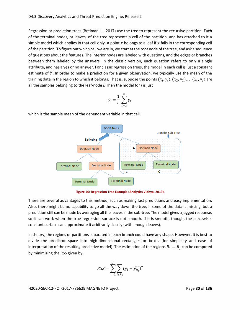
D4.3 Discovery Analytics and Threat Prediction Engine, Release 2
H2020-SEC-12-FCT-2017-786629 MAGNETO Project Page 80 of 136
Regression or prediction trees (Breiman L. , 2017) use the tree to represent the recursive partition. Each
of the terminal nodes, or leaves, of the tree represents a cell of the partition, and has attached to it a
simple model which applies in that cell only. A point 𝑥 belongs to a leaf if 𝑥 falls in the corresponding cell
of the partition. To figure out which cell we are in, we start at the root node of the tree, and ask a sequence
of questions about the features. The interior nodes are labeled with questions, and the edges or branches
between them labeled by the answers. In the classic version, each question refers to only a single
attribute, and has a yes or no answer. For classic regression trees, the model in each cell is just a constant
estimate of 𝑌. In order to make a prediction for a given observation, we typically use the mean of the
training data in the region to which it belongs. That is, suppose the points (𝑥𝑖, 𝑦𝑖), (𝑥2, 𝑦2), . . . (𝑥𝑐 , 𝑦𝑐) are
all the samples belonging to the leaf-node i. Then the model for i is just
�̂� =1
𝑐 ∑𝑦𝑖
𝑐
𝑖=1
which is the sample mean of the dependent variable in that cell.
Figure 40: Regression Tree Example (Analytics Vidhya, 2019).
There are several advantages to this method, such as making fast predictions and easy implementation.
Also, there might be no capability to go all the way down the tree, if some of the data is missing, but a
prediction still can be made by averaging all the leaves in the sub-tree. The model gives a jagged response,
so it can work when the true regression surface is not smooth. If it is smooth, though, the piecewise-
constant surface can approximate it arbitrarily closely (with enough leaves).
In theory, the regions or partitions separated in each branch could have any shape. However, it is best to
divide the predictor space into high-dimensional rectangles or boxes (for simplicity and ease of
interpretation of the resulting predictive model). The estimation of the regions 𝑅1… 𝑅𝐽 can be computed
by minimizing the RSS given by:
𝑅𝑆𝑆 =∑∑(𝑦𝑖 − 𝑦𝑅𝑗)̂ 2
𝑖𝜖𝑅𝑗
𝐽
𝑖=1

D4.3 Discovery Analytics and Threat Prediction Engine, Release 2
H2020-SEC-12-FCT-2017-786629 MAGNETO Project Page 81 of 136
where 𝑦𝑅�̂� is the mean response for the training observations within the 𝑗-th region.
It is computationally infeasible to consider every possible partition of the feature space into 𝐽 regions. So,
a top-down approach called recursive binary splitting is being applied. It is called top-down since it begins
at the top of the tree (all observations below to a single region) and then successively splits the predictor
space using minimization of RSS to estimate the branches as mentioned above. Each split is indicated via
two new branches further down on the tree.
This method, however, needs to know when to stop splitting as it works its way down the tree with the
training data. The most common stopping procedure is to use a minimum count on the number of training
instances assigned to each leaf node. If the count is less than some minimum threshold, then the split is
not accepted and the node is taken as a final leaf node. However, this procedure ends up with a large tree.
So, in order to achieve better performance and reduction of the size, pruning can be applied to the tree.
More specifically, cost complexity pruning generates a series of trees 𝑇0, … , 𝑇𝑚 where 𝑇0 is the initial tree
and 𝑇𝑚 is the root alone. At step 𝑖, the tree is created by removing a sub-tree from tree 𝑖 − 1 and replacing
it with a leaf node with value chosen as in the tree building algorithm.
3.4.4 Evaluation
For the evaluation of the performance of the above regression models, we have used the CDR data
provided by IGPR. The data have been preprocessed in order to keep the information of one subscriber
(IMEI, IMSI). Multiple models based on the above algorithms have been implemented in order to learn
the pattern of the call durations (in minutes). For the implementation process the scikit-learn package
(scikit-learn: machine learning in Python, 2019) and the neupy package (Nepy - Neural Networks in
Python, 2019) have been used, while the negative value of the median absolute error has been used for
the evaluation of the models. The results are depicted in Table 9 and in the boxplot of Figure 41, where
the median absolute error refers to call duration in minutes.
Table 9: Results of regression models.
Model Median
absolute
error
(min)
Linear Regression 6.03
RIDGE Regression 4.03
LASSO Regression 4.42
Regression Trees 5.89
Artificial Neural Networks (ANN) (4-5-2-1) 4.42

D4.3 Discovery Analytics and Threat Prediction Engine, Release 2
H2020-SEC-12-FCT-2017-786629 MAGNETO Project Page 82 of 136
General Regression Neural Networks (GRNN)
(𝝈 = 𝟎. 𝟎𝟗)
3.63
From the obtained results it becomes obvious that GRNN outperforms the rest of the models. It should
be noted, that the performance of the above models will be evaluated by using more datasets and
different numbers of hidden layers and neurons for artificial neural networks.
Figure 41: Evaluation results of the regression models for predicting call duration in CDR dataset.
3.5 Feature Extraction and Anomaly Detection with Scalable Machine-
learning Methods
3.5.1 General Overview of the Proposed Concept
The proposed approach for distributed feature extraction and machine learning adopts the scalable data
processing framework that is fitted into the Magneto Big Data Foundation Service (see Figure 42). In
general, the data can be provided to the system in any machine-readable format. However, here we
consider how the proposed approach can be used to analyse CDR (Call Data Record) files in order to train
discriminative models for anomaly detection applications.

D4.3 Discovery Analytics and Threat Prediction Engine, Release 2
H2020-SEC-12-FCT-2017-786629 MAGNETO Project Page 83 of 136
The raw data is sent via ingestion node to Apache Kafka, which makes the data available for the modules
responsible for further analysis (in this case Apache Spark and Elasticsearch). The data ingestion tools
come with Apache Kafka framework as Kafka Connect component.
Nonetheless, the key element responsible for data processing shown in Figure 42 is Apache Spark. This
framework provides an engine that processes big data workloads. Apache Spark uses the data abstraction
called resilient distributed dataset (RDD) to manage the data distributed in the cluster and to implement
fault-tolerance.
In Apache Spark framework, there are several key elements of the architecture that facilitate the
distributed computing, namely:
node (or host) - is a machine that belongs to computing cluster,
driver (an application) - is a module that contains the application code and communicates with
the cluster manager,
master node (a cluster manager) - is the element communicating with the driver and responsible
for allocating resources across applications,
worker node - a machine that can execute application code and holds an executor,
Figure 42: Feature extraction and anomaly detection – processing pipeline overview
3.5.2 Data Pre-processing and Visual Analysis
Various patterns emerging from data can be searched visually by means of the Elasticsearch database. In
Figure 43, there are CDR files that have been ingested and indexed in the database. The index name has
following format:
magneto-<telco operator>-<type>-<msisdn>

D4.3 Discovery Analytics and Threat Prediction Engine, Release 2
H2020-SEC-12-FCT-2017-786629 MAGNETO Project Page 84 of 136
where “telco operator” stands for the name of the operator the CDR has been provided, “type” indicates
type of the file (either billings or BTS logs), and “msisdn” indicates the subscriber number for whom the
CDR has been requested.
Figure 43: CDR ingested into Elasticsearch DB
This data can be analyzed using Kibana system. The example of CDRs presented on the timeline has been
shown in Figure 44.
Figure 44: CDR visualized on timeline
One of the requirements in the test scenario (WSPOL, 2019) presented by WSPOL, indicates that one of
the MAGNETO tasks could be to visualise “the most frequent contacts of the provided phone numbers”.
This can be easily checked by filters applied on the data. In the Figure 44, we search for “48089245242”
number and we get an extensive list of all calls established by that number.

D4.3 Discovery Analytics and Threat Prediction Engine, Release 2
H2020-SEC-12-FCT-2017-786629 MAGNETO Project Page 85 of 136
Figure 45: Graph of calls counts in a time interval
We further narrow down the list of results using visualisation capabilities of the Kibana tool. One of the
examples is presented in Figure 46.
Figure 46: The most frequent contacts of the 48089245242 phone number

D4.3 Discovery Analytics and Threat Prediction Engine, Release 2
H2020-SEC-12-FCT-2017-786629 MAGNETO Project Page 86 of 136
The CDR records contain also information about the geo-location of the BTS (base transceiver stations).
This allows us to render the most frequent base stations the subscribed joined. The results are shown
Figure 47.
Figure 47: The CDRs related to number 48542385426 shown on the map.
3.5.3 Feature Extraction
Usually, the single CDR record does not provided enough information to represent user behaviour.
Commonly, various clustering techniques are used to group the CDR by timestamp and/or caller ID. For
such groups additional statistics can be calculated that potentially allows for describing interesting
patterns. Therefore, the proposed feature extraction method aggregates the call records in the time
windows. For each time window, the records are grouped by the window number and the subscriber
number (the phone number which initialised the call). Finally, for each group several statistics are
calculated. Currently, these include the number of calls, total number of unique phone numbers
contacted, as well as average, min, and max lengths of call. The general overview of this process has been
shown in Figure 48.

D4.3 Discovery Analytics and Threat Prediction Engine, Release 2
H2020-SEC-12-FCT-2017-786629 MAGNETO Project Page 87 of 136
Figure 48: The overview of feature extraction method.
3.5.4 Distributed Machine Learning
There are various ML techniques that could be potentially used in the presented example. However, here
we focus on two classifiers which are efficient, scalable by design, and are implemented in Apache Spark
framework.
The Random Forest (RF) classifier adapts a modification of the bagging algorithm. The difference is in the
process of growing the trees. Commonly the N training samples (each with M input variables) are sampled
with replacements to produce B partitions. Each of the B partitions is used to train one of the trees. Each
tree is grown (trained) in a classical way by introducing nodes that split data. In case of the Random Forest
classifier, the splitting point is selected only for a randomly chosen variable (m out of M available). Finally,
the prediction score obtained with the B trained trees can be calculated using majority vote.
There already exists a scalable implementation of the Random Forest classifier in the MLlib Apache Spark
library. It uses the distributed computing environment, so that the computation can be parallelised. In
practice, the learning process for each decision tree can be performed in parallel. Keeping in mind that
each tree is trained only on the subset of data; it leads to effective schema that scales up to a large
datasets.
More precisely, when the Random Forest is trained in the Apache Spark environment, the algorithm
samples (with the replacement) the learning data and assigns it to the decision tree, which is trained on
that portion of the data. However, the data samples are not replicated explicitly, but instead it is
annotated with the additional records that keep information about probability that given instance belongs
to specific data partition used for training.
The training process is coordinated centrally (at so-called master node) using a queue of trees nodes.
Therefore, several threes are trained simultaneously. For each node in the queue the algorithm searches
for the best split. At this stage cluster resources are engaged (so called worker nodes). The algorithm
terminates when the maximum height of the decision tree is reached or whenever there is no data point
that is misclassified. The final output produced by the ensemble is the majority vote of results produced
by the decision trees.

D4.3 Discovery Analytics and Threat Prediction Engine, Release 2
H2020-SEC-12-FCT-2017-786629 MAGNETO Project Page 88 of 136
The Distributed Gradient-Boosted Trees classifier is another example of machine learning technique that
scales very well. In contrast to the Random Forest Classifier (where many trees can be trained
simultaneously), the Boosted Trees Classifier uses an additive learning approach. In each iteration a single
tree is trained and is added to the ensemble in order to fix errors (optimise the objective function)
introduced in previous iteration. The objective function measures the loss and the complexity of the trees
comprising the ensemble. In order to handle the arbitrary loss function, common implementations of the
GBT algorithms adapt the second order Taylor expansion.
3.5.5 Evaluation
In the research area of the supervised classification, there exist principles for classifiers evaluation. In
particular, we have data that state a true output and a prediction produced by the evaluated classifier.
Therefore, for each data sample (which is labelled) we can check the classifier output (prediction) with
the expected value (true output), and calculate following measures:
True Positive (TP) – true output is positive and prediction is also positive
True Negative (TN) – true output is negative and prediction is also negative
False Positive (FP) – true output is negative but prediction is positive
False Negative (FN) – true output is positive but prediction is negative
These are used to calculate commonly used metrics such as:
Accuracy = (TP+TN)/N
Precision = TP/(TP+FP)
Recall = TP/(TP+FN)
F-score = 2*(Precision*Recal)/(Precision+Recal)
For the evaluation we used the WSPOL CDR dataset. We trained two classifiers to recognize malicious
behaviours using the statistics explained in the previous section. Here we assumed that the malicious are
the call details records, which are related to the heads of the organized group presented in the WSPOL
scenario. The quantitative results have been presented in Table 10.
Table 10: Evaluation of Random Forest classifier on WSPOL CDR dataset.
Method Accuracy
[%]
Precision
[%]
Recall
[%]
F-score
RF, 10 trees, 1 hour time
window
96.74 96.85 96.53 0.9653
RF, 10 trees, 15 minutes time 95.16 95.1 95.15 0.9487
GBT, 1 hour time window 96.85 96.79 96.85 0.9681
GBT, 15 minutes time 94.92 94.83 94.92 0.9464

D4.3 Discovery Analytics and Threat Prediction Engine, Release 2
H2020-SEC-12-FCT-2017-786629 MAGNETO Project Page 89 of 136
We have compared above-described two classifiers that are implemented in the SparkML library (Apache
Spark, MLlib: Main Guide - Spark 2.4.4 Documentation, 2019), namely GBT (Gradient-boosted Tree) and
RF (Random Forest). The results are reported for two time windows of different length (1 hour and 15
minus respectively). We have used “random split” methodology (randomSplit - Documentation for
package ‘SparkR’ version 2.1.3, 2019) to divide the CDR dataset into training and testing parts.
3.6 Multi-camera Person Detection and Tracking Video security monitoring has always been an important mission for safety reason. In an entire
surveillance system, there are usually several cameras distributed sparsely to cover a wide range of public
areas (e.g., school, shopping mall or infrastructure). Tracking person through the CCTV network is
challenging due to different camera perspectives, illumination changes and pose variations. Several
algorithms for Multi-Target Multi-Camera tracking (MTMCT) have been proposed in offline method which
has delay in getting result. Addressing the need for real-time computation of people tracks through multi-
camera, MAGNETO proposes an online tracking solution. This includes (1) online real-time framework, (2)
extend a single camera multi object tracking (MOT) algorithm designed for multi-camera tracking and (3)
use spatial-temporal information to strengthen cross camera person recall performance. The proposed
solution is evaluated by experimenting in a real-world multi-camera dataset.
3.6.1 Overview of Existing Work
Intelligent video surveillance has been one of the most active research areas in computer vision (Wang X.
, 2013). Most of works have been done for single camera multi object tracking (MOT). Several existing
Multi-Target Multi-Camera Tracking (MTMCT) algorithms reported in literature are based on offline
method which requires to consider before and after frames to merge tracklets, and do post processing to
merge the trajectory. In the literature, hierarchical clustering (Z. Zhang, 2017) and correlation clustering
(Tomasi, 2018) are reported for merging the bounding box into tracklets from neighbor frames. In that
case, the tracking is hysteresis (delay in outputting final results) which cannot track the person in-time
and get the current exact location.
Addressing the need to generate real-time tracker without the apriori knowledge of person tracks, an
online real-time MTMCT algorithm has been developed, which aims to track a person cross camera
without overlap through a wide area. The framework performs a person detection based on Openpose (Z.
Cao, 2016), building on a multi-camera tracker extended by a single camera tracker MOTDT (L. Chen,
2018). The novelty of the proposed solution relies on adding a new tracking state. Due to the variation
among different perspective of different cameras, the appearance feature is not robust enough to
associate person cross camera. To address this issue, the spatial-temporal information is used to mitigate
the influence of different views. The main difference of the proposed framework is its online and real-
time performance comparing to other online tracker.
3.6.1.1 Person Re-Identification
The research on person re-identification has attracted attention from several researchers focused on the
development of reliable tracking algorithm. Person Re-ID has been regarded as a classification problem

D4.3 Discovery Analytics and Threat Prediction Engine, Release 2
H2020-SEC-12-FCT-2017-786629 MAGNETO Project Page 90 of 136
or verification problem. Classification problem uses ID or attributes as labels to train the network, while
the verification problem is aim to determine whether the two images belong to one person. The loss
function is design to make the distance of the positive pair as small as possible. Common methods are
contrastive loss (Varior, Haloi, & Wang, 2016), triplet loss (D. Cheng, 2016) and quadruplet loss (W. Chen,
2017). In order to improve the performance, lots of research focus on local feature instead of the global
feature of the whole person, such as slice (R. R. Varior, 2016), pose and skeleton alignment (L. Zheng,
2017). While matching local features help to improve in Person Re-ID, the challenge of pose variation
remain open due to the different view from camera.
3.6.1.2 Multi-Object Tracking
Multi-target tracking (MOT) aims to simultaneously locate and track multiple targets of interest in the
video, maintain the trajectory and record the ID. Compare to single object tracking, there are two more
challenges: the number of targets varies with time, maintain the ID of the targets. MOT algorithms can be
broadly classified into two categories namely (i) online and (ii) offline (W. Luo, 2014). The online tracking
only consider the information of previous and present frame and use current observations to extend
existing trajectories gradually. While offline tracking can use future information, which can link several
observations into trajectories but has a delay in the final result output.
3.6.1.3 Cross Camera Association
Compared to single camera tracking, multi-camera tracking need to associate the same ID through
different cameras without overlapping. For person association, person re-ID features (Tomasi, 2018) and
simple average color histogram (K. Yoon, 2019) are used. In addition to appearance feature, the spatial
and temporal information based on the position of cameras also can be considered (Chen, Huang, & Tan,
2014). Although some of multi-camera tracker have a good performance, they are offline framework,
which cannot get result in real-time for practical use. Addressing the influence of pose variation, triplet
loss and part-alignment (L. Zhao, 2017) are used to train the feature extraction network by learning to
align local parts of interest. In order to build a real-time online framework, the online tracker MOTDT (L.
Chen, 2018) is used to do single camera tracking. We extend it to be a multi-camera tracker. To enhance
the performance of multi-camera association by overcoming the current limitation of perspective
variation, the spatial-temporal matrix (G. Wang, 2018), which was used in Re-ID task, are implemented in
MTMC tracking task. The details are described in the next section.
3.6.2 Proposed Approach
In this online system, all cameras videos are processed together at the same time frame by frame in multi-
thread environment, without post-processing. The proposed algorithm for MTMC includes four stages. In
the first stage, person detection is obtained by Openpose (Z. Cao, 2016). Then, pose points extracted by
Openpose are transferred to bounding box coordinates. After refinement, the person feature of each
bounding box is extracted and set ID to each of them. In single camera, the tracklet is merged by
considering the appearance feature extracted by Re-ID network and motion feature extracted by Kalman
Filter. When the ID disappears in one camera, it will be placed into searching pool and may be reactivated
by one of the other cameras through its appearance features and spatialtemporal features. The spatial-
temporal probability metric is developed by a fast Histogram-Parzen (HP) method. The flow chart of the
whole process can be seen in Figure 49.
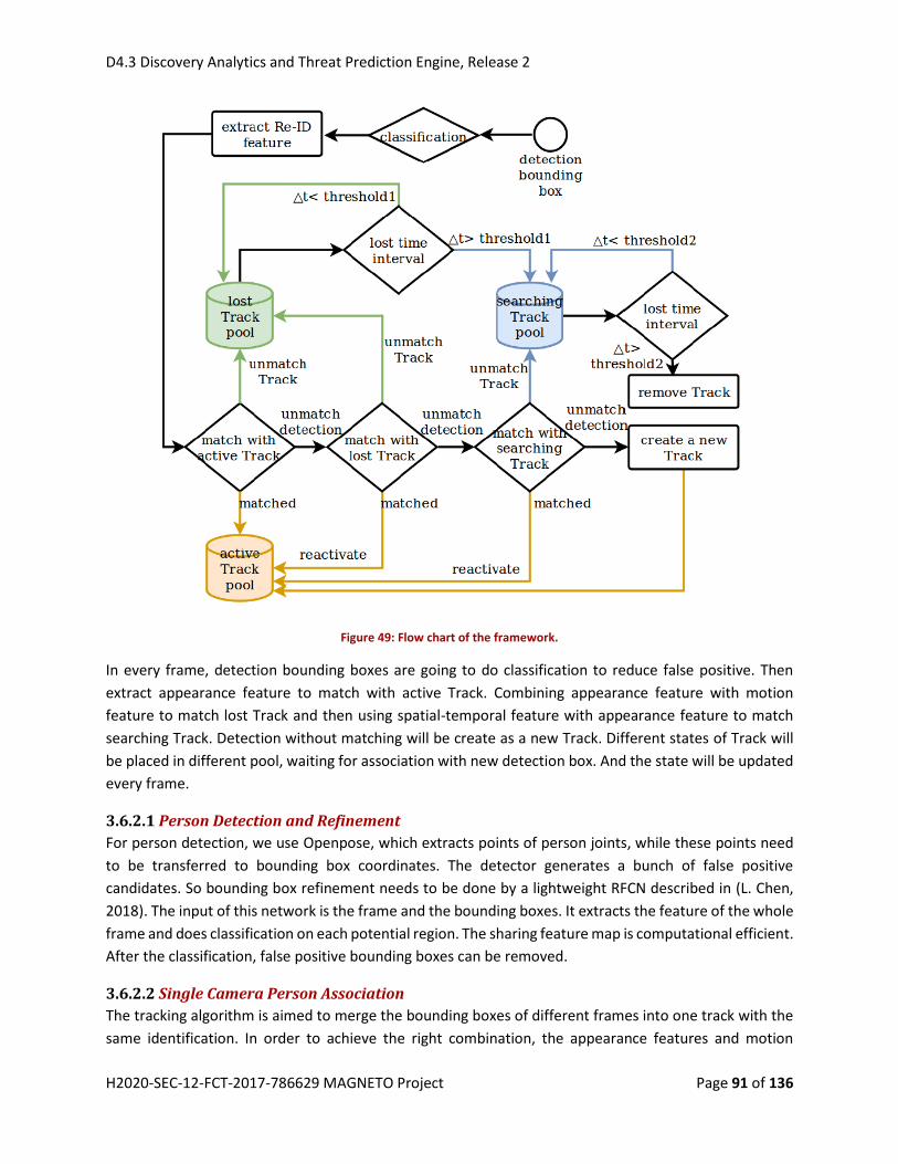
D4.3 Discovery Analytics and Threat Prediction Engine, Release 2
H2020-SEC-12-FCT-2017-786629 MAGNETO Project Page 91 of 136
Figure 49: Flow chart of the framework.
In every frame, detection bounding boxes are going to do classification to reduce false positive. Then
extract appearance feature to match with active Track. Combining appearance feature with motion
feature to match lost Track and then using spatial-temporal feature with appearance feature to match
searching Track. Detection without matching will be create as a new Track. Different states of Track will
be placed in different pool, waiting for association with new detection box. And the state will be updated
every frame.
3.6.2.1 Person Detection and Refinement
For person detection, we use Openpose, which extracts points of person joints, while these points need
to be transferred to bounding box coordinates. The detector generates a bunch of false positive
candidates. So bounding box refinement needs to be done by a lightweight RFCN described in (L. Chen,
2018). The input of this network is the frame and the bounding boxes. It extracts the feature of the whole
frame and does classification on each potential region. The sharing feature map is computational efficient.
After the classification, false positive bounding boxes can be removed.
3.6.2.2 Single Camera Person Association
The tracking algorithm is aimed to merge the bounding boxes of different frames into one track with the
same identification. In order to achieve the right combination, the appearance features and motion

D4.3 Discovery Analytics and Threat Prediction Engine, Release 2
H2020-SEC-12-FCT-2017-786629 MAGNETO Project Page 92 of 136
features are used. The appearance features are extracted by the part-align Re-ID network (Wang J. , 2018)
on each bounding box. The backbone of the network Hreid is GoogLeNet (C. Szegedy, 2014). It is connected
to K branches of fully-connected layers for part-alignment. The feature of candidate person I is f = Hreid(I).
The bounding boxes in the different frames will be merged into one track if the Euclidean distance dij,
between the two candidates Ii and Ij , is smallest among all the distances and within a threshold m. The
motion features are generated by a Kalman Filter, which predicts the position of a moving object. The
association will be removed if the distance of two bounding boxes exceeds the predicted area. When a
person is occluded by another person or obstacle, a Kalman filter can help to predict the trajectory of the
missing target. Moreover, when the person reappears, the lost track can be reactivated. When the track
is reactivated, the Kalman filter will be reinitialized, because the accuracy will decrease without update
over a long time.
3.6.2.3 Cross Camera Person Association
For multi-camera tracking, a person should be correctly associated with the previous Track. The
appearance feature, spatial and temporal feature is used to do the person association. The appearance
feature is extracted by person Re-ID network, and calculate the distance between the new target and the
features stored in the Track. A spatial-temporal probability metric (C. Szegedy, 2014) is used for helping
alleviate the problem of appearance ambiguity due to the perspective variation. The spatial-temporal
information can be learnt depends on the position of the camera. The time interval between different
cameras varies.
Figure 50 shows a track x of a person in camera i ending at time t0 and the system turning into searching
state. A candidate y in camera j at time t1 will match with Track x depends on the appearance feature and
time interval t0-t1 related to spatial information (camera transfer from i to j).
Figure 50: Camera transfer from cam I to cam j

D4.3 Discovery Analytics and Threat Prediction Engine, Release 2
H2020-SEC-12-FCT-2017-786629 MAGNETO Project Page 93 of 136
Figure 51: State transitions of a track
Figure 51 shows the state transitions of a track. Each Track has four states. At beginning, a track will be
active by create a new track. When the Track lost tracking and if the time interval smaller than the
threshold like t1, it will be reactive. If the time interval larger than the threshold like t2, it will change into
searching state. If the time period of searching state is larger than the threshold like t3, the Track will be
removed.
We summarized the histogram of time interval distribution of possible camera change and smoothed it
by the Parzen Window method. The probability of positive association pair is
k means the k-th bin of a histogram. ci and cj are the index of camera. 𝑛𝑐𝑖𝑐𝑖𝑗𝑘 represents the number of
person pairs disappearing from camera i and reappearing in camera j in k time intervals. y=1 when the
identity Ii and Ij is same. The histogram is smoothed by
K(.) is a Gaussian function kernel and 𝑍 = ∑ 𝑝(𝑦 = 1|𝑘, 𝑐𝑖, 𝑐𝑗)𝑘 is a normalized factor. Then the
appearance feature and spatial-temporal feature are integrate by Logistic Smoothing (LS) similarity
metric.
pjoint stand for 𝑝(𝑦 = 1|𝑥𝑖, 𝑥𝑗, 𝑘, 𝑐𝑖 , 𝑐𝑗), pst is 𝑝(𝑦 = 1|𝑘, 𝑐𝑖, 𝑐𝑗) and s is 𝑠(𝑥𝑖, 𝑥𝑗) which is the similarity score
of the appearance feature. f(.) is a logistic function:

D4.3 Discovery Analytics and Threat Prediction Engine, Release 2
H2020-SEC-12-FCT-2017-786629 MAGNETO Project Page 94 of 136
so that pjoint is robust enough for rare events, since the spatial-temporal probability if not reliable for every
situation.
Figure 52: Histogram of time interval (ID transfer from camera 2 to camera 1).
Figure 53: Camera topology of eight cameras.

D4.3 Discovery Analytics and Threat Prediction Engine, Release 2
H2020-SEC-12-FCT-2017-786629 MAGNETO Project Page 95 of 136
3.6.2.4 MTMC Tracker
Our tracker is an online tracker which runs in real-time without any post-processing. The single-camera
multi-object tracking algorithm is (L. Chen, 2018). We extend it to be suitable for multi-camera tracking.
Each person has his/her own track. Every track has information, such as track state, start tracking frame,
end tracking frame, which camera is the track belongs to, and 100 most recent appearance features of
the track. There are four different track states: active, lost, searching and removed, as shown in Figure 51.
Active means the person is being tracked in a single camera. Lost means the track is temporarily lost due
to occlusion by other person or obstacles. It will be reactivated soon if the time interval is within the
threshold. A track disappears in a camera will be marked as searching state. This kind of track will be put
into a searching pool. When a new person appears in a camera, it will be matched with the track in the
searching pool depends on the appearance feature and the spatial-temporal feature. A track disappears
longer than a threshold will be marked to be removed which will not be recalled by other cameras.
Figure 54 shows an experiment example with Person ID22 and ID23 in Camera2 at frame number 7299
(on the left), and in Camera1 at frame number 9312(on the right). This result shows the correct cross-
camera association.
Figure 54: Experiment example for correct cross camera association.
3.6.3 Experiments and Evaluation
3.6.3.1 Dataset Description
Experiments were run on DukeMTMC dataset (Tomasi, 2018), which contains 8 cameras with four
sequence: trainval, trainval-mini, test-easy and test-hard. The ground truth of testing set is unavailable,
so we use the ’trainval-mini sequence’ as testing set and the remaining of ’trainval sequence’ as training
set.
3.6.3.2 Experimental Setup
For appearance feature extraction, the network was trained based on DukeMTMC Re-ID dataset. The k in
part-align is 8. The network extracts 8 parts-align features inside the bounding box, and concatenates

D4.3 Discovery Analytics and Threat Prediction Engine, Release 2
H2020-SEC-12-FCT-2017-786629 MAGNETO Project Page 96 of 136
them together as a 512 dimension feature map. To learn spatial-temporal metric, the ground truth of
training set is used. For each ID, consider the first frame and the last frame in a certain camera. Then sort
the camera according to the frame number. Then calculate the time interval between different cameras,
and summarize the frequency in every 100 frames to get the histogram (shown in Figure 52 and Figure
53).
The experiment is executed with NVIDIA GeForce GTX 1060 6GB. The processing frame rate at testing
stage is 21fps with 8 cameras together. So it achieved real-time and online with high performance. Figure
54, Figure 55, and Figure 56 show samples from the evaluation results.
Figure 55: Multi-person detection on real CCTV footage.

D4.3 Discovery Analytics and Threat Prediction Engine, Release 2
H2020-SEC-12-FCT-2017-786629 MAGNETO Project Page 97 of 136
Figure 56: Multiple tracks detected across different CCTV cameras
3.6.3.3 Evaluation Protocol
In order to evaluate the performance, we follow the ID measures of performance in (Varior, Haloi, &
Wang, 2016). For ranking MTMC trackers, IDF1 is the principal measure which is the number of correctly
identified detection divided by the average number of computed and true detections. IDP and IDR are the
scores of true detections that are identified correctly.
3.6.3.4 Result and Discussion
Table 11 evaluates the multi-camera result with different configurations. The first two rows indicate the
detection bounding box that will influence the performance of tracking even after the refinement. The
reason is that the refinement network only performs classification without bounding box regression. And
the person Re-ID network relies on the coordinate to extract features. DPM generates a coarse bounding
box around a person with uncertain scale and ratio. The input of appearance feature extraction network
will meet problem such as: missing feet or hands, containing too many background and different aspect
ratio of the input. While Openpose generates 18 keypoints of the joints in a person. So, after transferring
the keypoints to four coordinates, the bounding box perfectly covers a person. So, the appearance
features are more robust to be matched.

D4.3 Discovery Analytics and Threat Prediction Engine, Release 2
H2020-SEC-12-FCT-2017-786629 MAGNETO Project Page 98 of 136
Table 11: Multi-camera result in different settings.
Detection Cross-camera
association
IDF1 IDP IDR
DPM Appearance
feature
45.41 47.43 43.56
Openpose Appearance
feature
47.34 48.95 45.84
Openpose Appearance + ST
feature
53.2 55.38 51.96
The comparison between the second row and the third row shows that the spatial temporal feature helps
to improve the performance of cross-camera matching. The second row only uses appearance feature to
do the identity association. The pose and perspective in different cameras are varied. For example, a
person in camera 4 is visible as a frontal view. When the person moves to camera 3, the view changes to
a side view. So, the appearance feature are changed that some of person may not be associated. The
spatial temporal matrix helps to mitigate the influence of pose variation.
Table 12 Multi-camera result comparison.
Method IDF1 IDP IDR
(Varior, Haloi, & Wang,
2016)
37.3 59.6 39.2
(Chen, Huang, & Tan,
2014)
50.1 58.3 43.9
Ours 53.2 55.38 51.96
The combination of appearance feature and spatial-temporal feature increases the match probability of
the right identity pair. The performance comparison with other models is shown in Table 12. Our models
outperform others in IDF1 and IDR.
The proposed multi-target multi-camera tracking algorithm enables real-time and online tracking of
pedestrians in CCTV footage. The results proved the detection bounding box will influence the
performance of appearance feature matching. And the spatial temporal information helps to mitigate the
adverse effect of pose variation between different cameras.

D4.3 Discovery Analytics and Threat Prediction Engine, Release 2
H2020-SEC-12-FCT-2017-786629 MAGNETO Project Page 99 of 136
3.6.3.5 Improvements to the person-fusion framework
One of the limitations of the MTMCT that was identified following the tool demonstration to LEA is the
inability of the solution to anchor specific person of interest (POI) to be used to retrieve and respective
appearance of the POI. This problem has been further exemplified with the demonstration of the DROP
component developed in WP3, where the LEAs expressed an interest to use the whole person as a query
example in retrieving the spatio-temporal appearance of people captured across various surveillance
cameras deployed across city. In this regard, the MTMCT component has been further developed to
include ‘unsupervised multi-camera person re-identification’ framework. The overall framework design of
the proposed framework is presented in Fehler! Verweisquelle konnte nicht gefunden werden.. The
support for media handler is extended to include international encoding standards such as MPEG-2 and
H.264 among others. The implementation of the person detection component relies on the use of Region
based Fully Connected Neural Network (RFCN), followed by the feature extraction of the detected person
with a set of deep-learning features. The deep-learning features extracted from the identified bounding
boxes are then subjected to the application of an unsupervised algorithm for clustering the people. The
processing of the deep-learning features are further exploited to ensure the LEAs can provide an anchor
image of a POI, to retrieve the appearance of the person across several surveillance cameras.
Figure 57 – Unsupervised multi-camera person reidentification (re-id)

D4.3 Discovery Analytics and Threat Prediction Engine, Release 2
H2020-SEC-12-FCT-2017-786629 MAGNETO Project Page 100 of 136
Figure 58 - Key idea for RFCN network design
The implementation of the person detection component uses the RFCN network pre-trained and
customized to detect the people from several types of background contexts such as urban, landscape, etc.
The novelty of the RFCN network relies in the consideration of two-stage object detection strategy namely
(i) region proposal and (ii) region classification. The scientific rationale behind the use of the two-stage
proposal is elaborated in (Dai, He, & Sun, 2016).Following the extraction of the regions (RoIs), the R-FCN
architecture is designed to classify the RoIs into object categories and background. In R-FCN, all learnable
weight layers are convolutional and are computed on the entire image. The last convolutional layer
produces a bank of 𝑘2position-sensitive score maps for each category, and thus has a 𝑘2(𝐶 + 1) - channel
output layer with 𝐶 object categories (+1 for background). The bank of 𝑘2 score maps correspond to a
𝑘 × 𝑘 spatial grid describing relative positions. For example, with 𝑘 × 𝑘 = 3 × 3, the 9 score maps
encode the cases of {top-left, top-center, top-right, ..., bottom-right} of an object category. R-FCN ends
with a position-sensitive RoI pooling layer. This layer aggregates the outputs of the last convolutional layer
and generates scores for each RoI. In comparison with the literature (He, Zhang, Ren, & Sun, 2014)
(Girshick, 2015), the position sensitive RoI layer in RFCN conducts selective pooling, and each of the 𝑘 × 𝑘
bin aggregates responses from only one score map out of the bank of 𝑘 × 𝑘 score maps. With end-to-end
training, this RoI layer shepherds the last convolutional layer to learn specialized position-sensitive score
maps. The architecture and the implementation of key ideas of RFCN network is presented in Fehler!
Verweisquelle konnte nicht gefunden werden..
Subsequent to the extraction of the people, the next steps is to extract deep-learning features from the
blobs that are identified as people. As noted earlier, the topic of person re-identification has been largely
applied to monitoring crowd without any intervention. Thus, for the purposes of MAGNETO project,
where the LEAs are only concerned tracking a specific individual, such as person of interest, it is vital to
adopt the solution to identify the anchor points, which are provided as input to the system. To address
such a need, the use of unsupervised clustering is carried out, to cluster the blobs extracted from the

D4.3 Discovery Analytics and Threat Prediction Engine, Release 2
H2020-SEC-12-FCT-2017-786629 MAGNETO Project Page 101 of 136
RFCN network. Subsequently, the features used is also able to provide the LEAs to identify and select a
specific person who is considered a POI for the identification across multiple cameras. The
implementation of the feature extraction has been carried out using two deep-learning network models
namely (i) RESNET-18 resulting in the deep-learning feature of length 1.x 512 and (ii) Alexnet deep learning
feature resulting in the feature length of 1x4096.
For the overall evaluation of the proposed unsupervised clustering framework, a set of videos across
London has been captured with actors playing the role of person of interest. A total of 5-clips has been
recorded. The map of the recorded footage collected in London is presented in Fehler! Verweisquelle
konnte nicht gefunden werden., along with some of the examples of MAGNETO actors passing through
the city in Fehler! Verweisquelle konnte nicht gefunden werden..
The experimental results of the component included a cluster size of 50 for each of the video footage, and
the aggregated result of the people detector was clustered using K-Means using both the RESNET-18 and
Alexnet deep-learning features. The results achieved 96% accuracy in each cluster for the 4-actors
embedded within the MAGNETO content capture. Subsequent analysis will be carried out for the
evaluation of the retrieval performance for each of the anchor as selected by the LEA.
Figure 59 - Map of data collection carried out within MAGNETO

D4.3 Discovery Analytics and Threat Prediction Engine, Release 2
H2020-SEC-12-FCT-2017-786629 MAGNETO Project Page 102 of 136
Figure 60 - Examples images of actors traversing the city
Figure 61 - Results of unsupervised clustering for multi-camera tracking
3.7 Language Models for Evidence Association The analysis of evidence and creating links between associated information obtained from heterogeneous
data sources is a crucial research activity. In the context of the MAGNETO, the processing of evidence
collected through witness reports among other external information data repository is represented as
linguistic resources. The problem of evidence association is treated as topic modelling as reported in the
literature, in which various groups of information are clustered and classified into a single topic model. As

D4.3 Discovery Analytics and Threat Prediction Engine, Release 2
H2020-SEC-12-FCT-2017-786629 MAGNETO Project Page 103 of 136
noted by Kuang et al (Kuang, Brantingham, & Bertozzi, 2017) in 2017, crimes often emerge out of a
complex mix of behaviors and situations. Therefore, the information that is required to represent and
summarize the category of the event into a single topic class presents a unique challenge. The expected
information loss from the category assignment impacts the ability of EU LEAs to not only understand the
causes of crime, but also how to develop optimal crime prevention strategies. Thus, the problem of
evidence association and crime category assignment is addressed using machine learning methods that
are applied on short narrative text descriptions accompanying crime records with the goal of discovering
ecologically more meaningful latent crime classes. The complexity of criminal activity modelling requires
the association of information into crime topics in reference to text-based topic modelling methods, which
can be further used to populate and instantiate the knowledge repository models. The representation of
criminal actions replicate broad distinctions between violent and property crime within MAGNETO, but
also reveal nuances linked to target characteristics, situational conditions and the tools and methods of
attack. The characteristics of the criminal types and behavior models are formalized as not discrete in
topic space. Rather, crime types are distributed across a range of crime topics. Similarly, individual crime
topics are distributed across a range of formal crime types. Key ecological groups include identity theft,
shoplifting, burglary and theft, car crimes and vandalism, criminal threats and confidence crimes, and
violent crimes. Though not a replacement for formal legal crime classifications, crime topics provide a
unique window into the heterogeneous causal processes underlying crime.
In the literature, topic models have been widely used to discover latent semantic structures within large
corpus of information. The topic structures in corpora have certain theoretical and practical value. In
addition to Latent Semantic Analysis (LSA) and Latent Dirichlet Allocation (LDA) for textual language
modelling, researchers have also proposed Correlated Topic Model (CTM) (Blei & Lafferty, Correlated
Topic Models, 2005). These algorithms have been used in different techniques and assumptions to analyze
a corpus. The three algorithms although complementary between each other, addresses topic modelling
separately. While LSA applies Singular Value Decomposition (SVD) to reduce dimensions of documents,
Probabilistic Latent Semantic Analysis (PLSA) is an extension of LSA from the perspective of probability.
LDA introduces Dirichlet prior for generating a document’s distribution over topics and gives a way to
model new documents. CTM models’ topic correlation between documents by replacing Dirichlet priors
with Logistic Normal priors. These algorithms have reported success in traditional tasks of large-corpus
analysis, which are then be applied to specific application on text classification and clustering (Cai, Mei,
Han, & Zhai, 2008), information retrieval (Chemudugunta, Smyth, & Steyvers, 2007), semantic analysis
(Lin & He, 2009).
The topic of text characterization in documents has been studied by the information retrieval and
statistical natural language processing for more than two decades. The key challenge that are commonly
addressed in the field of text analysis include classification, filtering and searching across a large collection
of documents. In recent years, the algorithms such as Probabilistic Latent Semantic Analysis (PLSA)
(Hofmann, 1999) and Latent Dirichlet Allocation (LDA) (Blei, Ng, & Jordan, Latent Dirichlet Allocation,
2003) have been identified as strong contenders for learning semantic representations for a large corpus.
Both techniques assume that each document has a multinomial distribution over topics and that each
topic is a mixture of distribution over words (Wang, Liu, Huang, & Feng, 2016). While these techniques

D4.3 Discovery Analytics and Threat Prediction Engine, Release 2
H2020-SEC-12-FCT-2017-786629 MAGNETO Project Page 104 of 136
have been successful in uncovering topics from general text documents, the distinctive characteristics of
tweets brings a set of new challenges and thus opportunities to develop novel solutions while analysis
tweets. The analysis of the results is presented by Wang et al. (Wang, Liu, Huang, & Feng, 2016), first, the
severe sparsity problem of tweet corpora (keeping in mind, the tweets retrieved from the platform are
selected based on an unknown ranking algorithm, which is influenced by the temporal characteristics of
the actual posts and the number of re-tweeters received) invalidates traditional topic modelling
techniques. Typically, LDA and PLSA both reveal the latent topics by identifying the word co-occurrence
patterns commonly found among the large corpus.
While the traditional NLP tools and systems have treated the words as atomic units - there is no notion of
similarity between words, as these are represented as indices in a vocabulary (Mikolov, Chen, Corrado, &
Dean, 2013). This choice has several good reasons - simplicity, robustness and the observation that simple
models trained on huge amounts of data outperform complex systems trained on less data. An example
is the popular N-gram model used for statistical language modeling - today, it is possible to train N-grams
on virtually all available data (trillions of words (Brants, Popat, Xu, Och, & Dean, 2007)). However, the
simple techniques are at their limits in many tasks. For example, the amount of relevant in-domain data
for automatic speech recognition is limited - the performance is usually dominated by the size of high-
quality transcribed speech data (often just millions of words). In machine translation, the existing corpora
for many languages contain only a few billions of words or less. Thus, there are situations where simple
scaling up of the basic techniques will not result in any significant progress, and a crucial need to develop
advanced techniques have been presented in (Mikolov, Sutskever, Chen, Corrado, & Dean, 2013) . With
progress of machine learning techniques in recent years, it has become possible to train more complex
models on much larger dataset, and they typically outperform the simple models. Probably the most
successful concept is to use distributed representations of words (Rumelhart & McClelland, 1986). For
example, neural network-based language models significantly outperform N-gram models (Bengio,
Ducharme, Vincent, & Janvin, 2003), (Schwenk, 2007), (Mikolov, Deoras, Kombrink, Burget, & Cernocký,
2011). In the rest of the subsection, a brief outline of three techniques namely Continuous Bag of Words
(CBOW), Continuous Skip-Gram and skip-gram model representation for textual feature extraction is
presented.
3.7.1.1 Continuous Bag of Words (CBOW) Model
In (Mikolov, Chen, Corrado, & Dean, 2013), the authors propose an architecture represents an extension
of the Neural Network Language Model (NNLM) like feedforward network, where the non-linear hidden
layer is removed and the projection layer is shared for all words (not just the projection matrix); thus, all
words get projected into the same position (their vectors are averaged). The authors have referred to the
architecture as a Bag-of-Words (BoW) model as the order of words in the history does not influence the
projection. Furthermore, the architecture also supports the use words from the future. The best
performance from the architecture has been extracted by building a log-linear classifier with four future
and four history words at the input, where the training criterion is to correctly classify the current (middle)
word. Training complexity is then
𝑄 = 𝑁 × 𝐷 + 𝐷 × 𝑙𝑜𝑔2(𝑉)
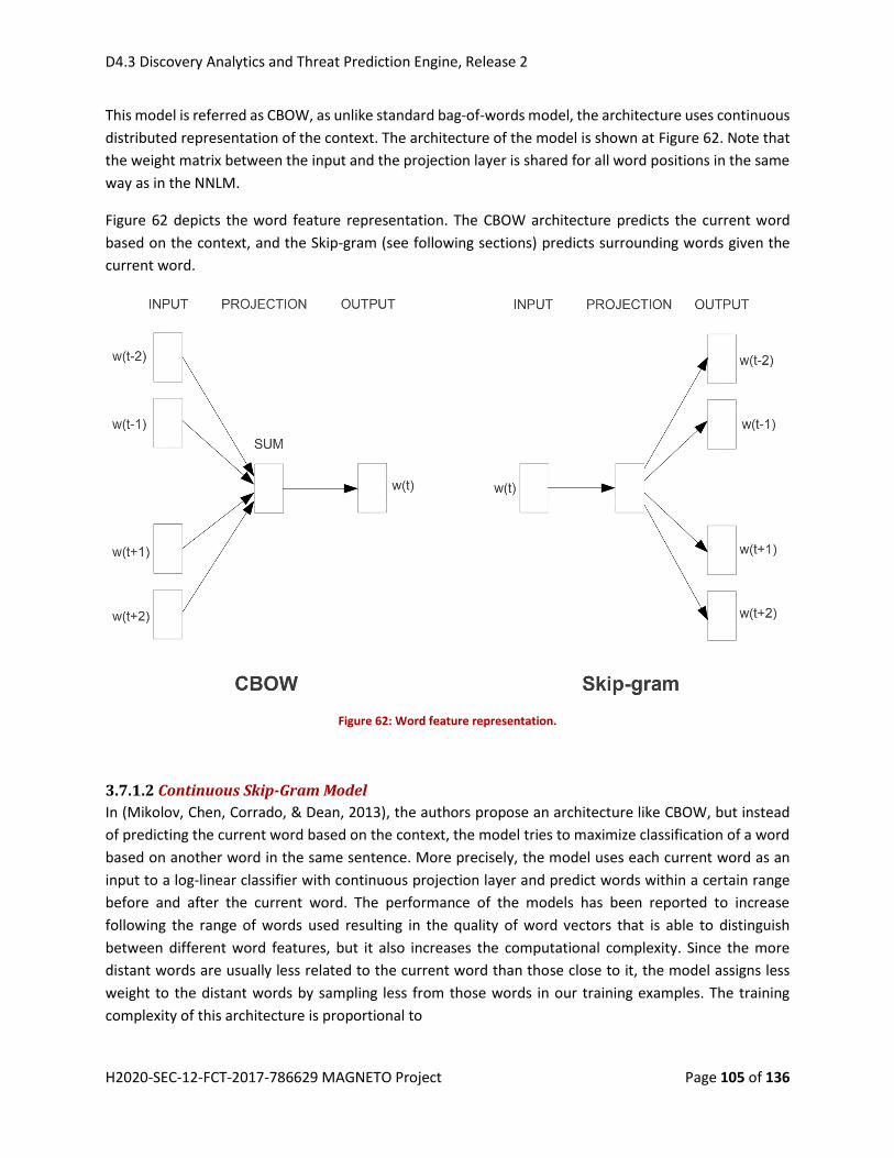
D4.3 Discovery Analytics and Threat Prediction Engine, Release 2
H2020-SEC-12-FCT-2017-786629 MAGNETO Project Page 105 of 136
This model is referred as CBOW, as unlike standard bag-of-words model, the architecture uses continuous
distributed representation of the context. The architecture of the model is shown at Figure 62. Note that
the weight matrix between the input and the projection layer is shared for all word positions in the same
way as in the NNLM.
Figure 62 depicts the word feature representation. The CBOW architecture predicts the current word
based on the context, and the Skip-gram (see following sections) predicts surrounding words given the
current word.
Figure 62: Word feature representation.
3.7.1.2 Continuous Skip-Gram Model
In (Mikolov, Chen, Corrado, & Dean, 2013), the authors propose an architecture like CBOW, but instead
of predicting the current word based on the context, the model tries to maximize classification of a word
based on another word in the same sentence. More precisely, the model uses each current word as an
input to a log-linear classifier with continuous projection layer and predict words within a certain range
before and after the current word. The performance of the models has been reported to increase
following the range of words used resulting in the quality of word vectors that is able to distinguish
between different word features, but it also increases the computational complexity. Since the more
distant words are usually less related to the current word than those close to it, the model assigns less
weight to the distant words by sampling less from those words in our training examples. The training
complexity of this architecture is proportional to

D4.3 Discovery Analytics and Threat Prediction Engine, Release 2
H2020-SEC-12-FCT-2017-786629 MAGNETO Project Page 106 of 136
𝑄 = 𝐶 × (𝐷 + 𝐷 × log2(𝑉))
where 𝐶 is the maximum distance of the words. Thus, if we choose C = 5, for each training word we will
select randomly a number 𝑅 in range < 1; 𝐶 >, and then use 𝑅 words from history and 𝑅 words from
the future of the current word as correct labels. This will require us to do 𝑅 × 2 word classifications, with
the current word as input, and each of the 𝑅 + 𝑅 words as output.
3.7.1.3 The Skip-gram Model
In (Mikolov, Sutskever, Chen, Corrado, & Dean, 2013), the authors proposed the architecture of a skip-
gram model. The training objective of the Skip-gram model is to find word representations that are useful
for predicting the surrounding words in a sentence or a document. More formally, given a sequence of
training words 𝑤1,𝑤2,𝑤3, . . . , 𝑤𝑇 the objective of the Skip-gram model is to maximize the average log
probability
1
𝑇∑ ∑ log𝑝(𝑤𝑡+𝑗|𝑤𝑡)
−𝑐≤𝑗≤𝑐,𝑗≠0
𝑇
𝑡=1
where 𝑐 is the size of the training context (which can be a function of the center word 𝑤𝑡). Larger 𝑐 results
in more training examples and thus can lead to a higher accuracy, at the expense of the training time. The
basic Skip-gram formulation defines 𝑝(𝑤𝑡 + 𝑗 |𝑤𝑡) using the softmax function:
𝑝(𝑊𝑂|𝑊𝐼) = exp (𝑣′𝑊𝑂
𝑇𝑣𝑊𝐼 )
exp (𝑣′𝑊𝑇𝑣𝑊𝐼 )
where 𝑣𝑤 and 𝑣𝑤′ are the “input” and “output” vector representations of 𝑤, and 𝑊 is the number of words
in the vocabulary. This formulation is impractical because the cost of computing 𝛻 log 𝑝(𝑤𝑂|𝑊𝐼 ) is
proportional to 𝑊, which is often large (105–107 terms). The language model implemented for the
evidence association extends from the skip-gram model namely word2vec representation.
3.7.2 Dataset Description
The News Category Dataset (Kaggle Inc, 2019) contains around 200k news headlines from the year 2012
to 2018 obtained from HuffPost. The model trained on this dataset could be used to identify tags for
untracked news articles or to identify the type of language used in different news articles. A total of 41
individual categories has been identified and labelled in the dataset. An example of an entry related to
CRIME category is presented in Table 13.
Table 13: An example of entry from News Category Dataset related to Crime
category: CRIME
headline: There Were 2 Mass Shootings In Texas Last Week, But Only 1 On TV

D4.3 Discovery Analytics and Threat Prediction Engine, Release 2
H2020-SEC-12-FCT-2017-786629 MAGNETO Project Page 107 of 136
authors: Melissa Jeltsen
link:
https://www.huffingtonpost.com/entry/texas-amanda-painter-mass-
shooting_us_5b081ab4e4b0802d69caad89
short_description: She left her husband. He killed their children. Just another day in America.
date:2018-05-26
3.7.3 Results
The implementation of the word2vec model (Řehůřek, 2019) was carried out on 3405 sentences, which
are formed by combining the headline and short-description from the News Category Dataset associated
only to CRIME category. The training of the said model was carried out with the following
hyperparameters.
size=100; represents the feature vector dimensionality
window=5; the sizes of the windows around which the context word has been selected
min_count=3; minimum number of word occurrence in the dataset to be qualified for training
workers=10, no. of threads used in the training process
iter=5000; no. of iterations used as stopping criteria.
The output of trained model for associating criminal entities within the dataset is presented in Table 14
Table 14: Example of evidence association based on the word embedding features
Killer
[('killers', 0.3419575095176697), ("killer's", 0.3245435655117035), ('sexual', 0.30444246530532837),
('above', 0.2807193100452423), ('killing', 0.2804318368434906), ("killer'", 0.2778010666370392),
('rahami', 0.27018681168556213), ('nurse', 0.26996350288391113), ('charges.', 0.26685670018196106),
('army', 0.2648443579673767)]
Shootings
[('shootings.', 0.40458589792251587), ('shooting', 0.3834560215473175), ('shooting,',
0.3324010968208313), ('store,', 0.31687989830970764), ('slayings', 0.3167177140712738), ('ohio,',
0.31160086393356323), ('palm', 0.29371175169944763), ('persons', 0.2776518166065216), ('california,',
0.2714591324329376), ('banks', 0.27117595076560974)]
Guns
[('nra', 0.36708223819732666), ('dallas', 0.3407415449619293), ('drives', 0.31851470470428467),
('gotten', 0.3066619038581848), ('committed', 0.30639949440956116), ('communities',
D4.3 Discovery Analytics and Threat Prediction Engine, Release 2
H2020-SEC-12-FCT-2017-786629 MAGNETO Project Page 108 of 136
0.3019908666610718), ('stories', 0.2954747676849365), ('been', 0.29515478014945984), ('depot',
0.28665655851364136), ('followed', 0.2841983139514923)]
Surgical
[('park.', 0.4009864926338196), ('carbon', 0.38064971566200256), ('mask', 0.3733969032764435),
('guide', 0.3728063404560089), ('crash:', 0.3495902419090271), ('donated', 0.34258803725242615),
('sailor', 0.34005722403526306), ('monoxide', 0.33888500928878784), ('self-inflicted',
0.33678948879241943), ('robbery', 0.32954633235931396)]
Firearms
[('forms', 0.3351077437400818), ('homicides', 0.3199557065963745), ('wore', 0.310121089220047),
('stephen', 0.30924659967422485), ('stories', 0.307538777589798), ('filled', 0.30232781171798706),
('growing', 0.3010709881782532), ('matter', 0.2967361807823181), ('whom', 0.2947126626968384),
('history.', 0.29131537675857544)]
Felony
[('prostitution', 0.4049314558506012), ('murder,', 0.4026116728782654), ('misdemeanor',
0.3604690432548523), ('assault.', 0.30662891268730164), ('abuse', 0.30584779381752014), ('rapes',
0.3022002577781677), ('sinnett', 0.2977193593978882), ('manslaughter', 0.2953537702560425), ('tests',
0.2948700189590454), ('misconduct', 0.29134541749954224)]
Welfare
[('bed', 0.36210504174232483), ('gifts', 0.3354347050189972), ('office', 0.33263295888900757),
('attorneys', 0.32393527030944824), ('non-life-threatening', 0.32125699520111084), ('corruption',
0.3191882371902466), ('laws', 0.31653618812561035), ('protection', 0.3123900294303894), ('services',
0.30628830194473267), ('test', 0.3060813546180725)]
The proposed language models also integrate the POS (Natural Language Toolkit - NLTK 3.4.5
documentation, 2019) tagger and WordNet synset models for annotating the extracted words to enhance
the quality of the evidence association framework.

D4.3 Discovery Analytics and Threat Prediction Engine, Release 2
H2020-SEC-12-FCT-2017-786629 MAGNETO Project Page 109 of 136
4. Threat Prediction Engine
4.1 Machine-learning Techniques to Infer Spatio-temporal Trends
4.1.1 Concept and Use-Cases
The primary use case for this concept is to obtain the crime probability density for an area of interest. In
addition to that, with information like a timestamp and crime category the crime probability density can
be obtained for:
A certain time of day
For each crime category
For a combination of crime categories
For all crimes
For a combination of the above
Once the probability density is found, one can ask how likely a crime in the current region and time interval
can occur. This allows to detect crime hot-spots in the chosen area and thus planning police patrols in the
area where the local hot-spots are detected. Figure 63 visualizes the basic workflow of the concept.
Figure 63: Workflow in estimating the probability density
Over time, the LEA’s are able to detect a certain trend, where crime hot-spots are heading. In addition to
that, when sufficient data has been collected over an amount of time intervals, the algorithm uses the
data from the past, to predict the probability densities for some time intervals in the near future. This
allows LEA’s to get an estimation, where the crime hot-spots may go.
4.1.2 Dataset
Since there is no real dataset provided, the dataset consists of synthetically generated data. It is assumed,
that in a specific area of interest, for example a city, crimes are recorded over a period of time and then
saved to a dataset along with their category, geolocation (longitude and latitude) and timestamp. For
further analysis, the dataset can be expanded by additional features.
4.1.3 Probability Density Estimation
Suppose we have a dataset of points on a map, where each point represents a crime. The data is recorded
in ascending adjacent time intervals of equal finite length 𝑡0, … , 𝑡𝑛, … 𝑡𝑁−1. The result is a point-cloud for
each time interval on a map within an area of interest 𝐴, where the crime incidents form several clusters,
like for example in Figure 64.

D4.3 Discovery Analytics and Threat Prediction Engine, Release 2
H2020-SEC-12-FCT-2017-786629 MAGNETO Project Page 110 of 136
Figure 64: Crime incidents at various locations in a defined area of interest
For each time interval 𝑡𝑛, the unknown function 𝑓𝑛(𝑥, 𝑦) represents the spatial probability density of the
point-cloud of crimes, which have occurred within 𝑡𝑛. The probability density, which we assume to be
square integrable, is approximated by a linear combination 𝑝(𝑥, 𝑦, 𝐶𝑛) of orthonormal3 basis functions
𝜙𝑚(𝑥, 𝑦) with respect to the 𝐿2 scalar product (𝑔, ℎ) = ∫ 𝑔(𝑥, 𝑦)ℎ(𝑥, 𝑦) 𝑑(𝑥, 𝑦)𝐴
:
𝑓𝑛(𝑥, 𝑦) ≈ 𝑝(𝑥, 𝑦, Cn) = ∑ 𝑐𝑛,𝑚
𝑀−1
𝑚=0
𝜙𝑚(𝑥, 𝑦)
The coefficient 𝑐𝑛,𝑚 controls the influence of the 𝑚-th basis function on the overall approximation of 𝑓𝑛.
The 𝑀 coefficients for the 𝑛-th time interval of the function approximation to be determined are
represented by the coefficient vector:
Cn = (𝑐𝑛,0, 𝑐𝑛,1, … , 𝑐𝑛,𝑀−1)
Neglecting the indices for the time interval 0, … , 𝑁 − 1, the probability density for one time interval can
be written as:
𝑓(𝑥, 𝑦) ≈ 𝑝(𝑥, 𝑦, 𝐶) = ∑ 𝑐𝑚𝜙𝑚(𝑥, 𝑦)
𝑀−1
𝑚=0
Then, given a family of 𝐿 data points with coordinates (𝑥𝑙 , 𝑦𝑙) for 𝑙 = 0,… , 𝐿 − 1, that represent the point
cloud, the 𝑚-th coefficient for the corresponding basis function can be approximated by the sum over the
results obtained by inserting all 𝐿 data points into the 𝑚-th basis function, divided by the number of data
points:
3 Orthonormal functions have the following characteristics:
𝜙𝑖 and 𝜙𝑗 are orthogonal, i.e. ∫ [𝜙𝑖(𝑥, 𝑦)][𝜙𝑗(𝑥, 𝑦)] 𝑑(𝑥, 𝑦) = 0 𝑓𝑜𝑟 𝑖 ≠ 𝑗𝐴 and
All 𝜙𝑖 are normalized, i.e. ∫ [𝜙𝑖(𝑥, 𝑦)]2𝑑(𝑥, 𝑦) = 1
𝐴

D4.3 Discovery Analytics and Threat Prediction Engine, Release 2
H2020-SEC-12-FCT-2017-786629 MAGNETO Project Page 111 of 136
𝑐𝑚 = (𝑓, 𝜙) ≈1
𝐿∑𝜙𝑚(𝑥𝑙, 𝑦𝑙)
𝐿−1
𝑙=0
For 𝐴 being of the form 𝐴 = [𝑎, 𝑏] × [𝑐, 𝑑], possible basis functions 𝜙𝑚(𝑥𝑙 , 𝑦𝑙) can be for example tensor
products of scaled:
Trigonometric polynomial or sine / cosine functions
Legendre polynomials
The probability density for time interval 𝑡𝑛 can be visualized as a “heat-map” that shows the crime
hotspots in the specified area 𝐴 within the time interval 𝑡𝑛. The contour lines of the heat-maps generated
from the point-clouds in Figure 64 are shown in Figure 65.
Figure 65: Heat-Maps for each time interval, generated from the corresponding point clouds in Figure 64
4.1.4 Probability Density Prediction
By approximating the function 𝑓𝑛(𝑥, 𝑦) by 𝑝(𝑥, 𝑦, 𝐶n), a set of parameters 𝐶𝑛 = (𝑐𝑛,0, 𝑐𝑛,1, … , 𝑐𝑛,𝑀−1) for
a single time interval 𝑛 is calculated. Calculating the coefficients over all 𝑁 time intervals, the coefficients
can be summarized in a coefficient matrix as follows:
𝑪𝟎 at interval 𝒕𝟎 𝑪𝟏 at interval 𝒕𝟏 … 𝑪𝑵−𝟏 at interval 𝒕𝑵−𝟏
𝒎 = 𝟎 𝑐0,0 𝑐1,0 … 𝑐𝑁−1,0
𝒎 = 𝟏 𝑐0,1 𝑐1,1 … 𝑐𝑁−1,1
𝒎 = 𝟐 𝑐0,2 𝑐1,2 … 𝑐𝑁−1,2
… … … … …
𝒎 = 𝑴− 𝟏 𝑐0,𝑀−1 𝑐1,𝑀−1 … 𝑐𝑁−1,𝑀−1
Each parameter 𝑚 has its own evolution over discrete time points within an interval 𝑇𝑝𝑎𝑠𝑡, so this trend,
for example like in Figure 66, can be used to extrapolate the coefficients onto a future time interval
𝑇𝑓𝑢𝑡𝑢𝑟𝑒.

D4.3 Discovery Analytics and Threat Prediction Engine, Release 2
H2020-SEC-12-FCT-2017-786629 MAGNETO Project Page 112 of 136
Figure 66: Evolution of coefficient cn,m, followed by the extrapolated coefficients (dotted line)
The extrapolation of the 𝑚-th coefficient is achieved by fitting a polynomial via a least square’s
approximation. The evaluation of this polynomial at a future point in time yields the 𝑚-th coefficient in
the basis expansion of the probability density at that time. Thus, coefficients for future time intervals with
𝑛 = 𝑁,𝑁 + 1,𝑁 + 2,… are obtained. The extrapolated coefficients are then used to establish linear
combinations of the basis functions 𝜙𝑚 which constitute estimates of the probability densities
corresponding to time intervals in the near future.
4.2 Machine learning techniques to detect abnormal activities
4.2.1 Approach
By accumulating the number of crimes, as described in 4.2.2, one can identify a possible trend and
seasonality in the observations. Assuming enough data, the evolution of the number of crimes, for
example in the next few months, can be forecasted out of the patterns, included in the past observations.
Moreover, extraordinary in- or decreases in (forecasted) crime-rates can be detected to give an alert to
the LEA’s, if desired. The general approach with the basic function blocks and their results are shown in
Figure 67.
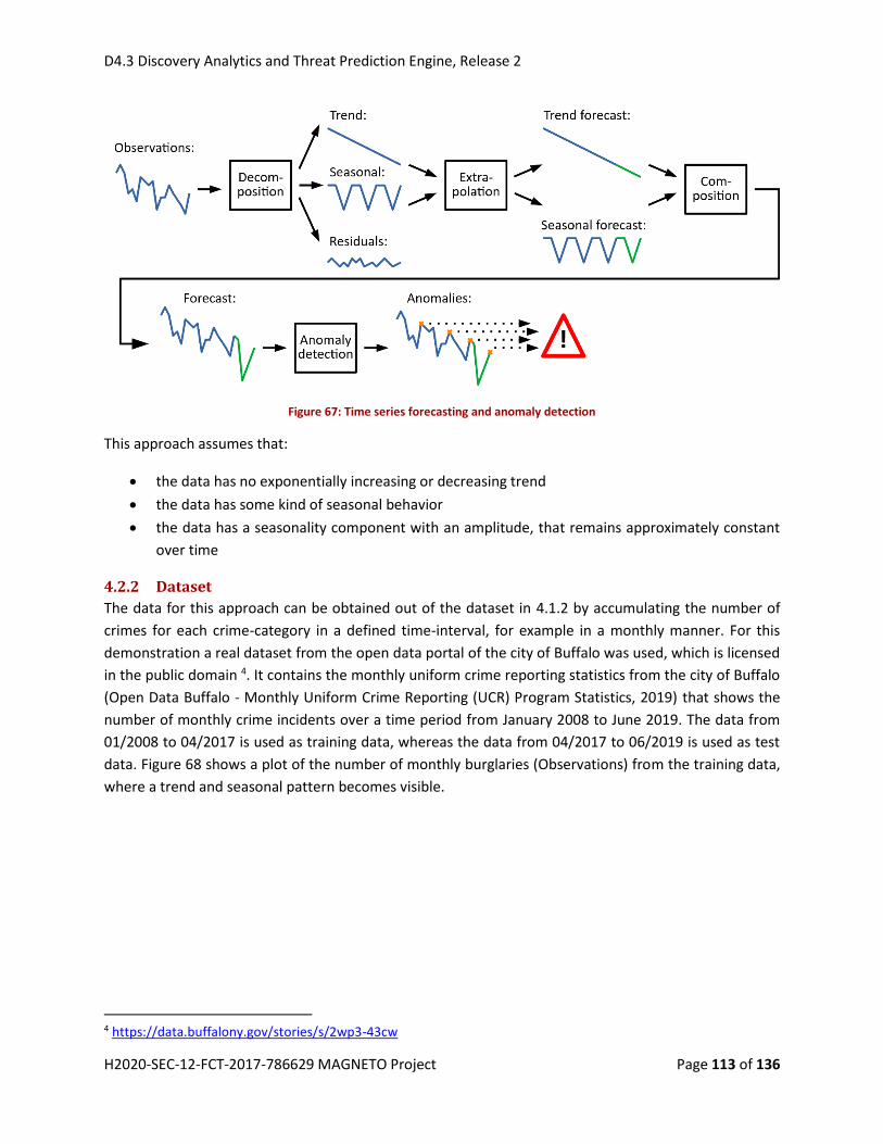
D4.3 Discovery Analytics and Threat Prediction Engine, Release 2
H2020-SEC-12-FCT-2017-786629 MAGNETO Project Page 113 of 136
Figure 67: Time series forecasting and anomaly detection
This approach assumes that:
the data has no exponentially increasing or decreasing trend
the data has some kind of seasonal behavior
the data has a seasonality component with an amplitude, that remains approximately constant
over time
4.2.2 Dataset
The data for this approach can be obtained out of the dataset in 4.1.2 by accumulating the number of
crimes for each crime-category in a defined time-interval, for example in a monthly manner. For this
demonstration a real dataset from the open data portal of the city of Buffalo was used, which is licensed
in the public domain 4. It contains the monthly uniform crime reporting statistics from the city of Buffalo
(Open Data Buffalo - Monthly Uniform Crime Reporting (UCR) Program Statistics, 2019) that shows the
number of monthly crime incidents over a time period from January 2008 to June 2019. The data from
01/2008 to 04/2017 is used as training data, whereas the data from 04/2017 to 06/2019 is used as test
data. Figure 68 shows a plot of the number of monthly burglaries (Observations) from the training data,
where a trend and seasonal pattern becomes visible.
4 https://data.buffalony.gov/stories/s/2wp3-43cw

D4.3 Discovery Analytics and Threat Prediction Engine, Release 2
H2020-SEC-12-FCT-2017-786629 MAGNETO Project Page 114 of 136
Figure 68: Number of monthly burglaries with trend from the beginning of 2008 to the end of 2017
4.2.3 Time series forecasting
Time series decomposition: A time series is an equally spaced set of observations, ordered by time, for
example monthly observations, as seen in Figure 68. An additive or multiplicative time series
decomposition (Hyndman & Athanasopoulos, 2018) assumes, that the underlying time series 𝑦𝑡 at the
period 𝑡 consists out of three components: A trend 𝑇𝑡, seasonality 𝑆𝑡 and the residuals 𝑅𝑡. The additive
model is given by
𝑦𝑡 = 𝑇𝑡 + 𝑆𝑡 + 𝑅𝑡 ,
whereas the multiplicative model is denoted by
𝑦𝑡 = 𝑇𝑡 𝑆𝑡 𝑅𝑡 .
A trend is a long- or short-term increase or decrease in the observations. The seasonal component is a
pattern in the time-series that repeats periodically after specific time intervals. Finally, the residual
component contains the “rest” or the “noise” of the time-series.
If the trend of the time series is exponentially increasing or the amplitude of the seasonal part is growing
over time, then a multiplicative model should be chosen, otherwise the additive model is more
appropriate. Using a logarithmic data transformation, the variation in the signal over time can be
stabilized, and the multiplicative model turns into an additive model:
𝑦𝑡 = 𝑇𝑡 𝑆𝑡 𝑅𝑡 → log(𝑦𝑡) = log(𝑇𝑡) + log(𝑆𝑡) + log(𝑅𝑡)
Assuming that in this use case the number of crimes is not exponentially increasing or decreasing and the
amplitude of the seasonal part remains constant over time, an additive model is used for time series
decomposition. For decomposing the time series into trend, seasonality and residuals a classical seasonal

D4.3 Discovery Analytics and Threat Prediction Engine, Release 2
H2020-SEC-12-FCT-2017-786629 MAGNETO Project Page 115 of 136
decomposition (Hyndman & Athanasopoulos, 2018) using moving averages is performed. The additive
decomposition has the following steps:
The trend �̂�𝑡 is obtained by a moving average filter. This can be realized via convolving the time-
series 𝑦𝑡 with a suitable filter-kernel (e.g. a low-pass filter that consists of a rectangular pulse with
an area of one), the window size of which depends on the frequency of the data in the time series.
Then, the time series is detrended by subtracting the trend from the observations:
�̂�𝑡 = 𝑦𝑡 − �̂�𝑡
A seasonal component results from the average of the detrended series for each time-period. For
monthly data, like in this case, the seasonal component for a certain month is the average of all
detrended values in the dataset from that month. For example, if one has a time series from
January 2008 to December 2010 and the detrended values for January are
�̂�𝑡=2008−01 = 19 ; �̂�𝑡=2009−01 = 15 ; �̂�𝑡=2010−01 = 21 ,
then the seasonal component for January is
�̂�𝑡=01∗ =
�̂�𝑡=2008−01 + �̂�𝑡=2009−01 + �̂�𝑡=2010−013
=19 + 15 + 21
3= 18,33
After that, all seasonal components are adjusted in a way, so they add to zero. One season is the
result of stringing together the individual seasonal components. Finally, repeating one season
periodically delivers the seasonal signal �̂�𝑡.
After subtracting the seasonal component from the detrended time series, the residuals �̂�𝑡
remain:
�̂�𝑡 = �̂�𝑡 − �̂�𝑡 = 𝑦𝑡 − �̂�𝑡 − �̂�𝑡
Figure 69 shows the observed number of burglaries from the dataset of 4.2.2, the trend 𝑇𝑡 as well as the
seasonality 𝑆𝑡 with a period of one year and the residuals 𝑅𝑡.

D4.3 Discovery Analytics and Threat Prediction Engine, Release 2
H2020-SEC-12-FCT-2017-786629 MAGNETO Project Page 116 of 136
Figure 69: Time-series decomposition of the Buffalo monthly UCR data
Alternatively a “Seasonal and Trend decomposition using Loess” (STL) algorithm could be used, which was
originally developed in 1990 by Cleveland et al (Cleveland, Cleveland, McRaw, & Terpenning, 1990) or
“RobustSTL” (Wen, et al., 2018), for robust long time series decomposition, which is more capable
handling abrupt trend changes shifts, and deals with seasonality shifts, fluctuations and noises.
Trend Extrapolation: Regarding the forecasting capabilities, by fitting a polynomial to �̂�𝑡 using the least
squares method, the Trend can be extrapolated beyond the range of the known data. The principle is the
same as for linear regression, which is used in 4.2.4, except the model, that is from a higher order, where
𝑑 is the degree of the polynomials:
𝑦𝑛 = 𝛽0 + 𝛽1𝑥𝑛 + 𝛽2𝑥𝑛2 +⋯+ 𝛽𝑑𝑥𝑛
𝑑 + 𝜀𝑛, 𝑛 = 1,2, … ,𝑁 .
However, initial experiments have shown, that interpolating within the known data range with splines and
subsequent extrapolation is more robust and flexible. Spline interpolation uses a piecewise polynomial to
interpolate the data between two data points (𝑥𝑘 , 𝑦𝑘) and (𝑥𝑘+1, 𝑦𝑘+1). A Spline 𝑆𝑃𝑘(𝑥) of degree 1
simply draws a line between two data points as shown in Figure 69 and has the following form:
𝑆𝑃𝑘(𝑥) =𝑦𝑘+1 − 𝑦𝑘
𝑥𝑘+1 − 𝑥𝑘(𝑥 − 𝑥𝑘) + 𝑦𝑘

D4.3 Discovery Analytics and Threat Prediction Engine, Release 2
H2020-SEC-12-FCT-2017-786629 MAGNETO Project Page 117 of 136
Figure 70: Spline interpolation of degree 1
The trend line of the last time step can be continued in order to extrapolate. For this purpose, a smoothing
factor 𝑠 is used, which controls the number of data points through which is interpolated or extrapolated
(The SciPy community, 2019). With smoothing, a number of 𝐷 data points can be used for smoothing the
trend-extrapolation. 𝐷 will be increased, until the following smoothing condition is satisfied:
∑(𝑤𝑗 (𝑦𝑗 − 𝑆𝑃𝑗(𝑥𝑗)))2
𝐽−1
𝑗=0
≤ 𝑠 ,
Where 𝑤𝑗 is the weight for the 𝑗-th interpolation interval, 𝑦𝑗 is the value of 𝑗-th data point at position 𝑥𝑗
and 𝑆𝑃𝑗(𝑥𝑗) the interpolated value at 𝑥𝑗. With 𝑠 = 0 the smoothing condition applies immediately, so the
interpolated line goes through every data point and the extrapolated line is the continued line with the
same slope as the line that goes through the last two data points. By increasing 𝑠, the slope of the Spline
interpolation is affected by more and more data points and the slope of the extrapolation depends on the
slope of a number of the last 𝐷 data points. This brings the slope of the extrapolation closer to the mean
slope of the trend regarding to the last data points, as shown in Figure 71. By default, 𝑠 is the number of
data points in the observations and 𝑤𝑗 = 1. Figure 71 shows an illustration of five data points (𝑥0, 𝑦0) to
(𝑥4, 𝑦4) through which is interpolated and then extrapolated with 𝑠 = 0, 𝑠 = 5 and 𝑠 = 20, where 𝑤𝑗 is
set to 𝑤𝑗 = 1.
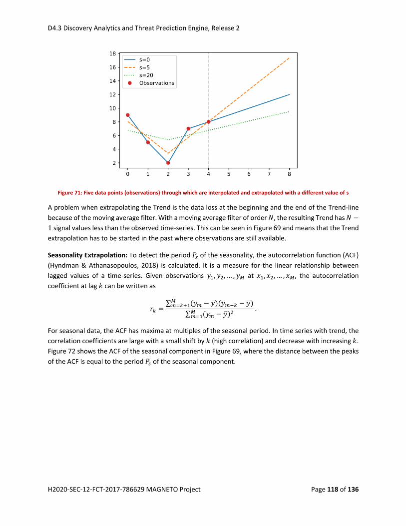
D4.3 Discovery Analytics and Threat Prediction Engine, Release 2
H2020-SEC-12-FCT-2017-786629 MAGNETO Project Page 118 of 136
Figure 71: Five data points (observations) through which are interpolated and extrapolated with a different value of s
A problem when extrapolating the Trend is the data loss at the beginning and the end of the Trend-line
because of the moving average filter. With a moving average filter of order 𝑁, the resulting Trend has 𝑁 −
1 signal values less than the observed time-series. This can be seen in Figure 69 and means that the Trend
extrapolation has to be started in the past where observations are still available.
Seasonality Extrapolation: To detect the period 𝑃𝑠 of the seasonality, the autocorrelation function (ACF)
(Hyndman & Athanasopoulos, 2018) is calculated. It is a measure for the linear relationship between
lagged values of a time-series. Given observations 𝑦1, 𝑦2, … , 𝑦𝑀 at 𝑥1, 𝑥2, … , 𝑥𝑀, the autocorrelation
coefficient at lag 𝑘 can be written as
𝑟𝑘 =∑ (𝑦𝑚 − �̅�)(𝑦𝑚−𝑘 − �̅�)𝑀𝑚=𝑘+1
∑ (𝑦𝑚 − �̅�)2𝑀
𝑚=1
.
For seasonal data, the ACF has maxima at multiples of the seasonal period. In time series with trend, the
correlation coefficients are large with a small shift by 𝑘 (high correlation) and decrease with increasing 𝑘.
Figure 72 shows the ACF of the seasonal component in Figure 69, where the distance between the peaks
of the ACF is equal to the period 𝑃𝑠 of the seasonal component.

D4.3 Discovery Analytics and Threat Prediction Engine, Release 2
H2020-SEC-12-FCT-2017-786629 MAGNETO Project Page 119 of 136
Figure 72: ACF of the seasonal component
As soon as 𝑃𝑠 is known, one period �̂�𝑡𝑝
from the seasonal part of the signal �̂�𝑡 can be extracted. To
extrapolate, �̂�𝑡𝑝
can be repeated periodically.
4.2.4 Anomaly detection
The goal of this part is to detect anomalies in the time series in form of sudden in- or decreases in signal
values with respect to the last 𝑁 time steps. An example for an anomaly is shown in Figure 73, where the
mean trend is decreasing and an incoming new observation is significantly outside a defined confidence
interval, which depends on the past 𝑁 observations.
Figure 73: Example for a new observation classified as an anomaly, based on the trend of a set of N=12 past observations within a 95% confidence interval

D4.3 Discovery Analytics and Threat Prediction Engine, Release 2
H2020-SEC-12-FCT-2017-786629 MAGNETO Project Page 120 of 136
With the proposed anomaly detection in combination with the forecasting capabilities in 4.2.1, a possibly
unexpected evolution of the observations can be automatically detected in order to give an alert, so this
will allow LEA’s to take appropriate measures if necessary.
Linear regression: To obtain a short-time trend (dashed line in Figure 73), a linear regression (Rencher &
Schaalje, 2008) is performed. The linear regression finds the trend-line, that best fits the last 𝑁
observations. The simple linear model for 𝑁 observations 𝑦1, 𝑦2, … , 𝑦𝑁 at 𝑥1, 𝑥2, … , 𝑥𝑁 is given by
𝑦𝑛 = 𝛽0 + 𝛽1𝑥𝑛 + 𝜀𝑛, 𝑛 = 1,2, … ,𝑁 .
Here, 𝛽0 and 𝛽1 are the model parameters and 𝜀𝑛 is the error term that holds the 𝑛-th residual. With the
estimated model parameters �̂�0 and �̂�1, the prediction is
�̂�𝑛 = �̂�0 + �̂�1𝑥𝑛 .
Then 𝜀𝑛 can be calculated by
𝜀𝑛 = 𝑦𝑛 − �̂�𝑛 .
Using the observations 𝑦1, 𝑦2, … , 𝑦𝑁 at 𝑥1, 𝑥2, … , 𝑥𝑁, the estimated model parameters �̂�0 and �̂�1 are
obtained by minimizing the residual sum of squares (𝑅𝑆𝑆). This procedure minimizes the error 𝜀𝑛2 between
the observed 𝑦𝑛 and the estimated �̂�𝑛:
𝑅𝑆𝑆 = ∑𝜀𝑛2
𝑁
𝑛=1
= ∑(𝑦𝑛 − �̂�𝑛)2
𝑁
𝑛=1
= ∑(𝑦𝑛 − (�̂�0 + �̂�1𝑥𝑛))2
𝑁
𝑛=1
→ 𝑚𝑖𝑛
To find �̂�0 and �̂�1 that minimize the 𝑅𝑆𝑆, the partial derivatives with respect to �̂�0 and �̂�1 are calculated,
which finally are set to zero:
𝜕𝑅𝑆𝑆
𝜕𝛽1= −2∑(𝑦𝑛 − (�̂�0 + �̂�1𝑥𝑛))𝑥𝑛 = 0
𝑁
𝑛=1
and
𝜕𝑅𝑆𝑆
𝜕𝛽0= −2∑(𝑦𝑛 − (�̂�0 + �̂�1𝑥𝑛)) = 0
𝑁
𝑛=1
,
which yields the regression coefficients
�̂�1 =∑ 𝑥𝑛𝑦𝑛 −𝑁�̅��̅�𝑁𝑛=1
∑ 𝑥𝑛2 −𝑁�̅�2𝑁
𝑛=1
and
�̂�0 = �̅� − �̂�1�̅� ,

D4.3 Discovery Analytics and Threat Prediction Engine, Release 2
H2020-SEC-12-FCT-2017-786629 MAGNETO Project Page 121 of 136
where �̅� is the mean of 𝑌, �̅� respectively:
�̅� =1
𝑁∑𝑦𝑛
𝑁
𝑛=1
.
Finally, the mean trend is extrapolated to �̂�𝑛 with 𝑛 = 1,2, … ,𝑁 + 1.
Variance: The variance 𝜎2 is an indicator, how far the 𝑁 past observations are spread over the y-axis and
is calculated by
𝜎2 =1
𝑁∑(𝑦𝑛 − �̅�)
2
𝑁
𝑛=1
,
Where the standard-deviation 𝜎 is the square-root of the variance.
Confidence interval: The confidence interval is the interval, in which most observations are falling.
Assuming a normal distribution, a 95% confidence interval of 2𝜎 says, that 95% of the observations are
within this interval. Figure 74 illustrates the 95% confidence interval, where the true mean �̅� is likely
between �̅� − 2𝜎 and �̅� + 2𝜎.
Figure 74: Confidence interval of 95% of a normal distribution
If �̂�1, �̂�2, … , �̂�𝑁+1 are the dependent variables of the extrapolated mean obtained from the observations
𝑦1, 𝑦2, … , 𝑦𝑁 and 𝑥1, 𝑥2, … , 𝑥𝑁+1 are the independent variables, the upper bound of the confidence
interval is calculated by
𝑢𝑛 = �̂�𝑛 + 2𝜎, 𝑛 = 1,2, … ,𝑁,𝑁 + 1 ,
and the lower bound of the 95% confidence interval by

D4.3 Discovery Analytics and Threat Prediction Engine, Release 2
H2020-SEC-12-FCT-2017-786629 MAGNETO Project Page 122 of 136
𝑙𝑛 = �̂�𝑛 − 2𝜎, 𝑛 = 1,2,… ,𝑁,𝑁 + 1 .
Anomaly detection: Finally, a new observation 𝑦𝑛=𝑁+1 is classified as an expected observation, if the
value 𝑦𝑛=𝑁+1 falls within the 𝑁 + 1-th confidence interval
𝑙𝑛=𝑁+1 ≤ 𝑦𝑛=𝑁+1 ≤ 𝑢𝑛=𝑁+1 ,
otherwise it is classified as an anomaly, when it lies outside of that interval. If such an anomaly has been
discovered, it is possible to give a hint to the user, if an extraordinary increase or decrease is detected.
Since extraordinary decreases, for example in the number of crimes, represent a positive development, it
is possible to ignore them.
4.2.5 Implementation
This approach was implemented in Python5 with NumPy6 for the basic computing and Matplotlib7 for
creating the graphs, where Pandas8 was used for loading and manipulating the data that is stored in a
CSV-file. The time series decomposition was realized with the Statsmodels9 module, where SciPy10 was
used for basic signal processing.
4.2.6 Evaluation
The result of the forecast and anomaly detection on the “Buffalo Monthly Uniform Crime Reporting”
dataset shows Figure 75, where ten extraordinary increases in the number of monthly crimes have been
detected. Extraordinary decreases were ignored. For calculating the linear regression and confidence
interval, a number of 𝑁 = 12 past observations have been used. The graph shows, that the predicted
number of crimes over 24 months is relatively close to the actual number of crimes from the test dataset.
5 https://www.python.org 6 https://numpy.org/ 7 https://matplotlib.org/ 8 https://pandas.pydata.org/ 9 https://pandas.pydata.org/ 10 https://www.scipy.org/

D4.3 Discovery Analytics and Threat Prediction Engine, Release 2
H2020-SEC-12-FCT-2017-786629 MAGNETO Project Page 123 of 136
Figure 75: Detected anomalies in the Buffalo Monthly Uniform Crime Reporting dataset with forecasted number of crimes compared to the number of crimes in the test data
The Root Mean Squared Error (𝑅𝑀𝑆𝐸) is an error-measure to compare the forecast of the model �̂�𝑛 with
the observed ground-truth value 𝑦𝑛 from the test dataset and is defined as
𝑅𝑀𝑆𝐸 = √1
𝑁𝑝∑(𝑦𝑛 − �̂�𝑛)
2
𝑁𝑝
𝑛=1
,
where 𝑁𝑝 is the total number of forecasted values. For a better interpretation, the RMSE can be
normalized by the mean �̅� of the values 𝑦𝑛 from the test data
𝑁𝑅𝑀𝑆𝐸 =𝑅𝑀𝑆𝐸
�̅� .
The 𝑅𝑀𝑆𝐸 / 𝑁𝑅𝑀𝑆𝐸 between the ground-truth and the forecast from 04/2017 – 06/2019 in Figure 75 is
𝑅𝑀𝑆𝐸 = 32,21
and
𝑁𝑅𝑀𝑆𝐸 = 0,1841 .
4.3 Complex Event Processing Events represent the most important resource of forensic knowledge because, thanks to its intrinsic
nature has many characteristics that are useful to model the MAGNETO forensic domain. Event (as
explained in D4.1) is a description of an incident or occurrence of some significance and may consist of a
number of smaller events and is therefore capable of sub-division.

D4.3 Discovery Analytics and Threat Prediction Engine, Release 2
H2020-SEC-12-FCT-2017-786629 MAGNETO Project Page 124 of 136
Complex event processing (CEP) is a novel technology with the purpose to identify complex events by
analyzing, filtering, and matching semantically low-level events. The main idea behind CEP systems lies in
identification of situations by examining the cause/effect relationships among simple events that carry no
specific information in stand-alone conditions. CEP techniques provide solid foundations on how to model
and evaluate logical structures of atomic event instances in order to detect (sequences or patterns of)
complex events. A basic event is atomic, indivisible and occurs at a point in time. Attributes of a basic or
atomic event are the parameters of the activity that caused the event. Atomic event instances can be
directly observed on an event stream while complex event instances are constituted from logic structures
of multiple atomic event instances, and thus, they cannot be directly observed. Instead, their presence is
deduced by processing the atomic event instances. Attributes of complex events are derived from the
attributes of the constituent basic events. Event constructors and event operators are used to express the
relationship among events and correlate events to form complex events. For example, the entry of an
identified person in a restricted area could be treated as an activity. Then the form of the event instance
could be composed by unique id of the person, time, and location (geographical coordinates).
Complex event processing means matching event instances against previously defined event patterns.
Event patterns are abstractions of event instances, and they are primarily characterized by the type and
potentiality. For example, the entry of an identified person in a restricted area could be treated as an
activity. Then the form of the event instance could be composed by unique id of the person, time, and
location (geographical coordinates). Events are related to each other though spatio-temporal relations
and complex events are composed of basic/ atomic events. Complex events are defined by connecting
basic/atomic events using temporal, spatial or logical relations.
A simple example is that of the unauthorized entry. When a person who does not possess a valid RFID
(Radio-frequency Identification) tag tries to enter a location just behind an authorized person it is called
as tailgating. This scenario can be captured through the CEP queries the wireless data for an event where
PIR (Processor Identification Register) is present but RFID is zero. Once such an event is identified, CEP
gets the image from the database corresponding to that event’s timestamp and gives the image to Face
Detection module. The Face detection algorithm counts the number of persons present and gives the
count back to CEP.
In MAGNETO systems, the basic/atomic events generated from heterogeneous sensors are collected,
aggregated using logical and spatiotemporal relations to form complex events which model the intrusion
patterns, so the need for multisensory data preprocessing is essential. The data pre-processing consists
of two main steps: (1) data integration and (2) generation of the set of instances and association rules.
For data integration step, the MAGNETO systems will fuse the heterogeneous data from the diverse data
sources after the initial pre-processing phase as described in D3.1. The goal of this fusion is to transform
lower-level data into higher-level quality information and to improve the certainty of situation
recognition. The fusion is realized by taking into consideration the semantics of the information. As
described in D4.1, event fusion tool in MAGNETO will use the Time and the Space concepts to represent
the moment and the place where the event took place and it relies on the use of bipartite graphs, more
specifically a subset of the conceptual graphs to represent semantic information and knowledge. Also,

D4.3 Discovery Analytics and Threat Prediction Engine, Release 2
H2020-SEC-12-FCT-2017-786629 MAGNETO Project Page 125 of 136
similarity functions are defined to compare the concept instances involved in the definition of an event,
such as Euclidean and Minkowski distance. Following the fusion of the initial data, MAGNETO system will
create the new instances and their attributes that will be used in the creation of the new semantic rules.
However, due to high velocity and the volume of these data, domain experts/LEAs cannot provide the
rules manually. Rule-based classifiers are the machine learning algorithms that can replace experts in
generating rule patterns and analyses those kinds of data. Such an algorithm is presented below.
4.3.1 Extracting Association Rules from CEP
In order to analyze the complex events, frequent itemset techniques are applied. Frequent itemset mining
leads to the discovery of associations and correlations among large datasets. Thus, if we consider the
itemset to be the set of events that consist a complex event, then such techniques, like the Apriori
algorithm, can be used to generate interesting association rules for the events under investigation. The
interestingness in the rules is expressed through rule support and confidence. These measures
respectively reflect the usefulness and the certainty of the discovered rules. A discovered rule may have
the following form:
Event 1 Event 2 [support 10%, confidence 60%]
In the above rule, the 10% support means that 10% of all the complex events contain Event 1 (E1) and
Event 2 (E2), while a confidence of 60% mean that 60% of the complex events that contain Event 1, also
contain Event 2. In mathematical terms, these measures can be expressed as follows:
𝑆𝑢𝑝𝑝𝑜𝑟𝑡(𝐸1 → 𝐸2) = 𝑃(𝐸1 ∪ 𝐸2)
𝐶𝑜𝑛𝑓𝑖𝑑𝑒𝑛𝑐𝑒(𝐸1 → 𝐸2) = 𝑃(𝐸2|𝐸1)
where
𝑃(𝐸2|𝐸1) = 𝑆𝑢𝑝𝑝𝑜𝑟𝑡(𝐸1 ∪ 𝐸2)
𝑆𝑢𝑝𝑝𝑜𝑟𝑡(𝐸1)=𝑠𝑢𝑝𝑝𝑜𝑟𝑡_𝑐𝑜𝑢𝑛𝑡(𝐸1 ∪ 𝐸2)
𝑠𝑢𝑝𝑝𝑜𝑟𝑡_𝑐𝑜𝑢𝑛𝑡(𝐸1)
Where 𝑠𝑢𝑝𝑝𝑜𝑟𝑡_𝑐𝑜𝑢𝑛𝑡(𝐸1 ∪ 𝐸2) is the number of complex events that contain events 𝐸1 ∪ 𝐸2, and
𝑠𝑢𝑝𝑝𝑜𝑟𝑡_𝑐𝑜𝑢𝑛𝑡(𝐸1) is the number of complex events containing 𝐸1.
Typically, association rules are considered interesting / strong, if they satisfy both a minimum support
threshold and a minimum confidence threshold. These thresholds should be a set by the LEA’s officers
who are domain experts. The generated rules can be later used for mining and extracting useful
information that will raise appropriate alarms if certain events are discovered.
As mentioned above, a powerful algorithm for discovering association rules is the Apriori algorithm
proposed by Agrawal and Srikant. Specifically, Apriori defines the frequent itemsets (i.e. events that occur
together) and extract the association rules using prior knowledge of frequent itemset properties. It
employs an iterative approach in which k-itemsets are used to explore (k+1) itemsets. First, the set of
frequent 1-itemsets is found by scanning the dataset to accumulate the count for each item, and collecting
those items that satisfy minimum support. The resulting set is denoted by L1. Next, L1 is used to find L2,

D4.3 Discovery Analytics and Threat Prediction Engine, Release 2
H2020-SEC-12-FCT-2017-786629 MAGNETO Project Page 126 of 136
the set of frequent 2-itemsets, which is used to find L3, and so on, until no more frequent k-itemsets can
be found. The finding of each Lk requires one full scan of the dataset. At each phase of transitioning from
Lk-1 to Lk, two steps are performed; a join step denoted as Ck in which joins Lk-1 with itself, and a prune step
which keeps only these items/events Lk that are frequent (i.e. satisfying a minimum support). It should be
noted that the search space at each phase is significantly reduced using the property of the Apriori which
states that “All nonempty subsets of a frequent itemset must also be frequent.”
After identifying the frequent itemsets/events from complex events in the dataset D, the rules are
generated from them using the equations described above for confidence and support. Specifically, the
process of generating the rules is:
For each frequent itemset/event l, generate all nonempty subsets of l.
For every nonempty subset s of l, output the rule “s (l-s)” if
𝑠𝑢𝑝𝑝𝑜𝑟𝑡_𝑐𝑜𝑢𝑛𝑡(𝑙)
𝑠𝑢𝑝𝑝𝑜𝑟𝑡_𝑐𝑜𝑢𝑛𝑡(𝑠)≥ min_conf
where min_conf is the minimum confidence threshold.
Because the rules are generated from frequent events, each one automatically satisfies the minimum
support, generating thus strong rules.
In order to illustrate how the algorithm works in MAGNETO, the following table consisting of events is
used. Specifically, the table describes 9 complex events each of which consists of several different
“simple” events (E1, …, E5). For instance, the first complex event CE_1 consists of the events E1, E2 and
E5. These complex events refer to more than one investigation cases that are handled by the LEAs and are
stored in the knowledge base of MAGNETO.
Table 15: List of events.
CE_ID List of events
CE_1 E1, E2, E5
CE_2 E2, E4
CE_3 E2, E3
CE_4 E1, E2, E4
CE_5 E1, E3
CE_6 E2, E3
CE_7 E1, E3
CE_8 E1, E2, E3, E5
CE_9 E1, E2, E3
Based on these events, the algorithm tries to find the k-itemsets. For the current example a minimum
absolute support of 2 has been used, which refers to a relative support of 2/9 =22%. Apriori finds the 1-
itemsets L1, the 2-itemsets L2 and the 3-itemsets L3, after which it terminates. This process is described in
Figure 76.

D4.3 Discovery Analytics and Threat Prediction Engine, Release 2
H2020-SEC-12-FCT-2017-786629 MAGNETO Project Page 127 of 136
Figure 76: Steps of the Apriori algorithm.
After identifying the frequent events, the rules can be easily derived. Assuming a complex event X = {E1,
E2, E5}, the association rules that can be generated from X contain all the nonempty subsets of X, i.e. {E1,
E2}, {E1, E5}, {E2, E5}, {E1}, {E2}, {E5}. The resulting association rules are:
i. {E1, E2} E5 with confidence = 50%
ii. {E1, E5} E2 with confidence = 100%
iii. {E2, E5} E1 with confidence = 100%
iv. {E1} {E2, E5} with confidence = 33%
v. {E2} {E1, E5} with confidence = 29%
vi. {E5} {E1, E2} with confidence = 100%
Finally, based on the confidence threshold set by the domain expert, only the strong rules will be
outputted.

D4.3 Discovery Analytics and Threat Prediction Engine, Release 2
H2020-SEC-12-FCT-2017-786629 MAGNETO Project Page 128 of 136
5. Conclusion
The toolbox for the processing of semantic information within the MAGNETO project, that had been
sketched in deliverable D4.2 has been further developed and expanded with the tools of the advanced
correlation engine. The tools have been designed to analyze and fuse information in order to help LEAs
aggregate information, detect correlations between the analyzed documents and infer new evidence from
the analysis of the knowledge.
The present deliverable D4.3 “Discovery Analytics and Threat Prediction Engine, Release 2” has presented
the methods and the design of the of MAGNETO’s advanced correlation engine. The implementation and
internal algorithms and functions of MAGNETO’s advanced correlation engine have been described. The
correlation engine uses a set of machine learning techniques to provide an overview to the large text and
data corpus by finding relations and detecting trends: Classification of datasets and clustering of natural
language texts, regression analysis, feature extraction and anomaly detection.
The semantic information processing and fusion tools that have been envisioned in deliverable D4.1 (ICCS,
IOSB, QMUL, SIV, TRT, 2019) have been developed and their architecture and functionality has been
described in detail. Two reasoning tools generate new knowledge by applying rules on the evidence stored
in the Common Representational Model (CRM):
The logical reasoning tool is based on the binary model of the evidence and its conclusions being
true or false.
The probabilistic reasoning tool is based on Markov Logic Network. A numerical confidence value
can be assigned both for the evidence and the rules, and the conclusions are also rated with a
confidence level.
In cooperation with the participating LEAs, rules have been implemented for several use cases: Diversion
Attacks, Examination of social relations, Fuel Crime - Decolourisation of Heating Oil, IED-Attacks,
Organized Crime.
The population of the CRM’s ontology with the inferred knowledge is illustrated and the implementation
of the ethical and legal requirements concerning explainability and court-proof evidence has been
achieved by annotating inferred relations with information about the rules used to create them.
The fusion tools generate knowledge by aggregation information that has been collected from various
sources. The fusion of a large number of location points to trajectories creates knowledge about the
movement of persons or vehicles. The received datasets of truck toll logs and Call Data Records (CDR)
have been investigated and used for evaluation. The person fusion’s objective is finding different person
instances in the knowledge graph that refer to the same person and fuse these instances. Several
techniques have been compared and tested that can be applied in order to improve the efficiency of the
tool For the purposes of MAGNETO, the early termination technique has been adopted for the Person
Fusion Tool.

D4.3 Discovery Analytics and Threat Prediction Engine, Release 2
H2020-SEC-12-FCT-2017-786629 MAGNETO Project Page 129 of 136
The Machine Learning Based Event Information Fusion will be able to classify events that are similar or
predict events using a cause-effect approach. The semantic information tools have been tested with some
exemplary datasets, giving an impression of what to expect in the application at the LEA premises.
The tools that build the correlation engine of MAGNETO have been introduced. The classification of
datasets has been based on the Decision Tree approach and has been applied to the financial dataset to
classify bank transactions to find suspicious transactions.
For clustering natural language text documents, three different algorithms have been tested and
compared on a small dataset. For the tested dataset, two of the algorithms (DBScan and KMeans++) have
outperformed over the other one (SIB). A human readable representation of the cluster content has been
proposed (tag crowd).
A tool for detecting outliers in a CDR-dataset has been developed that supports the integration of the
result into the CRM.
Model fitting techniques based on regression analysis have been presented to make predictions on the
future development of a system based on the history of observed parameters. Six regression methods
have been evaluated using the CDR data provided by IGPR.
The feature extraction and anomaly detection has been performed on Call Data Records using the
ElasticSearch-Kibana-Application and combining it with Apache Spark as a scalable data processing
framework that has been fitted into the Magneto Big Data Foundation Service.
The challenging task of tracking a person through the CCTV network has been addressed by the Multi-
Camera-Person-Detection tool providing solutions to the problem of person re-identification and cross-
camera association. An experimental setup has been established and the tests have shown that the multi-
target multi-camera tracking algorithm enables real-time and online tracking of pedestrians in CCTV
footage.
A method for the analysis of evidence has been presented that can create links between associated
information obtained from heterogeneous data sources. Different language models have been chosen
and compared with respect to the result achieved in an evaluation using a news test dataset.
The density-based approach of the Threat Prediction Engine enables the visualization and evaluation of
collected spatio-temporal crime-data and gives the ability to detect and predict spatio-temporal trends
and crime hot-spots. In addition to that, the proposed method of 4.2 give LEA’s the ability to infer and
predict the trend and seasonal behaviour of a certain crime category and make it possible to auto-detect
extraordinary in- or decreases in crime-rates. This allows preventive measures to be taken if necessary.
The test with a real dataset from the city of Buffalo has shown, that the monthly two-year forecast (in this
case) is relatively close to the real data from the test dataset. Furthermore, depending on the
configuration, the proposed method of section 4.2 is capable of reliably detecting exceptional increases
in crime-rates.

D4.3 Discovery Analytics and Threat Prediction Engine, Release 2
H2020-SEC-12-FCT-2017-786629 MAGNETO Project Page 130 of 136
Complex event processing (CEP) has been introduced to identify complex events by analyzing, filtering,
and matching semantically low-level events. It results in the identification of situations by examining the
cause/effect relationships among simple events that carry no specific information in stand-alone
conditions. It provides solid foundations on how to model and evaluate logical structures of atomic event
instances in order to detect (sequences or patterns of) complex events.

D4.3 Discovery Analytics and Threat Prediction Engine, Release 2
H2020-SEC-12-FCT-2017-786629 MAGNETO Project Page 131 of 136
6. Bibliography 68–95–99.7 rule - Wikipedia - Image. (2019, 09 23). Retrieved from
https://en.wikipedia.org/wiki/68%E2%80%9395%E2%80%9399.7_rule#/media/File:Empirical_rule_histogram.svg
A. Elmagarmid, P. I. (2007). Duplicate Record Detection: A Survey. IEEE Transactions on Knowledge and Data Engineering, Vol.19, No.1.
Analytics Vidhya. (2019, 09 23). What is a Decision Tree? How does it work? - | ClearPredictions.com. Retrieved from https://clearpredictions.com/Home/DecisionTree
Apache Spark, MLlib: Main Guide - Spark 2.4.4 Documentation. (2019, 09 23). Retrieved from https://spark.apache.org/docs/latest/ml-guide.html
Arlot, S., & Celisse, A. (2010). A survey of cross-validation procedures for model selection. Statistics Survey(Vol.4).
Bengio, Y., Ducharme, R., Vincent, P., & Janvin, C. (2003). A Neural Probabilistic Language Model. J. Mach. Learn. Res., 3, 1137--1155.
Bishop, C. (2011). Pattern Recognition and Machine Learning. Springer. Blei, D., & Lafferty, J. (2005). Correlated Topic Models. Proceedings of the 18th International Conference
on Neural Information Processing Systems. Vancouver, British Columbia, Canada. Blei, D., Ng, A., & Jordan, M. (2003). Latent Dirichlet Allocation. J. Mach. Learn. Res., 3, 993--1022. Brants, T., Popat, A., Xu, P., Och, F., & Dean, J. (2007). Large Language Models in Machine Translation.
Proceedings of the 2007 Joint Conference on Empirical Methods in Natural Language Processing and Computational Natural Language Learning ({EMNLP}-{C}o{NLL}). Prague, Czech Republic.
Breiman, L. (2017). Classification and Regression Trees. Chapman and Hall. Breiman, L., Friedman, J., Olshen, R., & Stone, C. (1984). Classification and regression trees. Monterey:
Brooks/Cole Publishing. C. Szegedy, W. L. (2014). Going deeper with convolutions. CoRR, vol. abs/1409.4842. Cai, D., Mei, Q., Han, J., & Zhai, C. (2008). Modeling Hidden Topics on Document Manifold. Proceedings
of the 17th ACM Conference on Information and Knowledge Management. Napa Valley, California, USA.
Chemudugunta, C., Smyth, P., & Steyvers, M. (2007). Modeling General and Specific Aspects of Documents with a Probabilistic Topic Model. In Advances in Neural Information Processing Systems 19 (pp. 241--248). MIT Press.
Chen, X., Huang, K., & Tan, T. (2014). Object tracking across non-overlapping views by learning inter-camera transfer models. Pattern Recognition, vol. 47(03), p. 1126-1137.
Chomboon, K., & al., e. (2015). An Empirical Study of Distance Metrics for k-Nearest Neighbor Algorithm. Proceedings of 3rd International Conference on Industrial Application Engineering. Japan.
Cleveland, R. B., Cleveland, W. S., McRaw, J. E., & Terpenning, I. (1990). STL. A Seasonal-Trend Decomposition Procedure Based on Loess. Journal of Official Statistics(6).
Computer Science Department Stanford. (2019, 09 19). Tuffy: A Scalable Markov Logic Inference Engine . Retrieved from Documentation: Learn more about Tuffy: http://i.stanford.edu/hazy/tuffy/doc/
D. Cheng, Y. G. (2016). Person reidentification by multi-channel parts-based cnn with improved triplet loss function. IEEE Conference on Computer Vision and Pattern Recognition (CVPR), 1335–1344.
Dai, J., He, K., & Sun, J. (2016). {R-FCN:} Object Detection via Region-based Fully Convolutional Networks. CoRR.
Doan, A., Niu, F., Ré, C., Shavlik, J., & Zhang, C. (2011, May 1). User Manual of Tuffy 0.3. Retrieved from http://i.stanford.edu/hazy/tuffy/doc/tuffy-manual.pdf
Draper, N., & H. Smith. (1998). Applied regression analysis. Wiley.

D4.3 Discovery Analytics and Threat Prediction Engine, Release 2
H2020-SEC-12-FCT-2017-786629 MAGNETO Project Page 132 of 136
EUROB, ITTI, VML, SIV, TRT, IOSB, ICCS, PAWA, CBRNE, QMUL, KUL, UPV. (2019). D2.3 Refined System Architecture and Representational Model.
G. Wang, J. L. (2018). Spatial-temporal person reidentification. CoRR, vol. abs/1812.03282. Girshick, R. (2015). Fast {R-CNN}. CoRR. Gorini M., C. V. (2013). EMERALD deliverable 'D2.3 - EMERALD System Functional Architecture'. Graphviz - Graph Visualization Software. (2019, 09 19). Retrieved from http://www.graphviz.org/ Haldar, R., & Mukhopadhyay, D. (2011). Levenshtein Distance Technique in Dictionary Lookup Methods:
An Improved Approach”. arXiv:1101.1232. He, K., Zhang, X., Ren, S., & Sun, J. (2014). Spatial Pyramid Pooling in Deep Convolutional Networks for
Visual Recognition. CoRR. Hernandez, M., & Stolfo, S. (1998, 01). Real-World Data Is Dirty: Data Cleansing and the Merge/Purge
Problem. Data Mining and Knowledge Discovery, vol. 2, no. 1, pp. 9-37. Hofmann, T. (1999). Probabilistic Latent Semantic Indexing. Proceedings of the 22Nd Annual
International ACM SIGIR Conference on Research and Development in Information Retrieval. Berkeley, California, USA.
Hyndman, R. J., & Athanasopoulos, G. (2018). Forecasting - Principles and Practice. Melbourne, Australia. ICCS, IOSB, QMUL, SIV, TRT. (2019). MAGNETO Deliverable D4.1: Semantic Reasoning and Information
Fusion Tools. ICCS, VML. (2019). Deliverable 6.1: Integrated Platform Release R0.5. Intuition of Gradient Descent for Machine Learning. (2019, 08 30). Retrieved from
https://medium.com/abdullah-al-imran/intuition-of-gradient-descent-for-machine-learning-49e1b6b89c8b
Java API for working with the SWRL rule and SQWRL query languages. (2019, 08 17). Retrieved from https://github.com/protegeproject/swrlapi
K. Hechenbichler, K. S. (2004). Weighted k-Nearest-Neighbor Techniques and Ordinal Classification. Retrieved from http://epub.ub.uni-muenchen.de/
K. Yoon, Y. S. (2019). Multiple hypothesis tracking algorithm for multi-target multi-camera tracking with disjoint views. CoRR, vol. abs/1901.08787.
Kaggle Inc. (2019, 09 23). News Category Dataset | Kaggle. Retrieved from https://www.kaggle.com/rmisra/news-category-dataset
Keen, B. (2019, 09 23). Generatedata.com: free, GNU-licensed, random custom data generator for testing software. Retrieved from https://www.generatedata.com/
Kenton, W. (2019, 09 23). Empirical Rule Definition (Inestopedia Academy). Retrieved from https://www.investopedia.com/terms/e/empirical-rule.asp
Khan, S. S., & Ahmad, A. (2013). Cluster center initialization algorithm for K-modes clustering. Expert Systems with Applications, 40, pp. 7444–7456,.
Kuang, D., Brantingham, P., & Bertozzi, A. (2017). Crime topic modeling. Crime Science, 6(1), 12. KUL, CBRNE. (2019). Ethical and Legal Guidelines for the use and development of MAGNETO Tools. L. Chen, H. A. (2018). Real-time multiple people tracking with deeply learned candidate selection and
person reidentification,” . CoRR, vol. abs/1809.04427. L. Zhao, X. L. (2017). Deeply-learned part-aligned representations for person re-identification. CoRR, vol.
abs/1707.07256. L. Zheng, Y. H. (2017). Pose invariant embedding for deep person re-identification. CoRR, vol.
abs/1701.07732. Li, H. (2019, 09 19). Smile - Statistical Machine Intelligence and Learning Engine. Retrieved from
https://haifengl.github.io/smile/data.html Lin, C., & He, Y. (2009). Joint Sentiment/Topic Model for Sentiment Analysis. Proceedings of the 18th
ACM Conference on Information and Knowledge Management. Hong Kong, China.

D4.3 Discovery Analytics and Threat Prediction Engine, Release 2
H2020-SEC-12-FCT-2017-786629 MAGNETO Project Page 133 of 136
Lloyd, J. W. (1987). Foundations of logic programming (second, extended edition). Springer series in symbolic computation. Springer-Verlag, New York, 1987.
M.J. O'Connor, R. S. (2008). The SWRLAPI: A Development Environment for Working with SWRL Rules. OWL: Experiences and Directions (OWLED), 4th International Workshop. Washington, D.C. , U.S.A.
Mikolov, T., Chen, K., Corrado, G., & Dean, J. (2013). Efficient Estimation of Word Representations in Vector Space. CoRR.
Mikolov, T., Deoras, A., Kombrink, S., Burget, L., & Cernocký, J. (2011). Empirical Evaluation and Combination of Advanced Language Modeling Techniques. INTERSPEECH.
Mikolov, T., Sutskever, I., Chen, K., Corrado, G., & Dean, J. (2013). Distributed Representations of Words and Phrases and their Compositionality. In Neural and Information Processing System (NIPS).
MINT, I. E. (2018). Deliverable 2.1: Uses Cases and Requirements. MAGNETO Project Consortium. Mitchell, T. (1997). Machine Learning (1st Edition ed.). McGraw-Hill. Montgomery, D., Peck, E., & Vining, G. (2012). Introduction to Linear Regression Analysis”. Wiley. Natural Language Toolkit - NLTK 3.4.5 documentation. (2019, 09 24). Retrieved from
https://www.nltk.org/ Nepy - Neural Networks in Python. (2019, 09 23). Retrieved from http://neupy.com/pages/home.html Open Data Buffalo - Monthly Uniform Crime Reporting (UCR) Program Statistics. (2019, 07 24). Retrieved
from https://data.buffalony.gov/Public-Safety/Monthly-Uniform-Crime-Reporting-UCR-Program-Statis/xxu9-yrhd
OWL API main repository. (2019, 08 17). Retrieved from https://github.com/owlcs/owlapi OWL API main repository. (2019, 08 17). Retrieved from https://github.com/owlcs/owlapi Pellet: An Open Source OWL DL reasoner for Java. (2019, 08 17). Retrieved from
https://github.com/stardog-union/pellet Philips, L. (1990, 12). Hanging on the Metaphone. Computer Language Magazine, vol. 7, no. 12, pp. 39-
44,. Retrieved from http://www.cuj.com/documents/s=8038/cuj0006philips/. Philips, L. (2000, 06). The Double Metaphone Search Algorithm. C/C++ Users J., vol. 18, no. 5. Porter, E. H., & Winkler, W. E. (1997). Advanced Record Linkage System. U.S. Bureau of the Census,
Research Report. Principal Component Analysis vs Ordinary Least Squares. (2019, 08 30). Retrieved from
https://cerebralmastication.com/2010/09/principal-component-analysis-pca-vs-ordinary-least-squares-ols-a-visual-explination/
QMUL, VML, ICCS, IOSB, UPV, PAWA, EUROB, SIV. (2019). Deliverable 3.2: Modular and Scalable Tools for Evidence Collection.
R. R. Varior, B. S. (2016). A siamese long short-term memory architecture for human re-identification,” . CoRR, vol. abs/1607.08381.
Rajaraman, A., & Ullman, J. (2011). In Data Mining: Mining of Massive Datasets” (pp. 1–17). randomSplit - Documentation for package ‘SparkR’ version 2.1.3. (2019, 09 23). Retrieved from
https://spark.apache.org/docs/2.1.3/api/R/randomSplit.html Regularization in Machine Learning. (2019, 08 30). Retrieved from
https://www.kdnuggets.com/2018/01/regularization-machine-learning.html Řehůřek, R. (2019, 09 23). gensim: Topic modelling for humans. Retrieved from
https://radimrehurek.com/gensim/ Rencher, A. C., & Schaalje, B. G. (2008). Linear Models in Statistics. John Wiley & Sons. Rumelhart, D., & McClelland, J. (1986). Parallel Distributed Processing: Explorations in the Microstructure
of Cognition, Vol. 1: Foundations. Cambridge, MA, USA: MIT Press. Saxena, A. (2019, 09 19). Implementing Decision Trees Using Smile. Retrieved from
https://dzone.com/articles/implementing-decision-tree-using-smile-scala

D4.3 Discovery Analytics and Threat Prediction Engine, Release 2
H2020-SEC-12-FCT-2017-786629 MAGNETO Project Page 134 of 136
Schwenk, H. (2007). Continuous Space Language Models. Comput. Speech Lang, 21(3), 492--518. scikit-learn: machine learning in Python. (2019, 09 23). Retrieved from https://scikit-learn.org/ Specht, D. (1991). A general regression neural network. IEEE Transactions on Neural Networks(vol. 2, no.
6). Sudhamathy, G., & Venkateswaran, C. J. (2019). R Programming: An Approach to Data Analytics. MJP
Publisher. Retrieved from https://books.google.de/books?id=1CebDwAAQBAJ SWRL: A Semantic Web Rule Language Combining OWL and RuleML. (2019, 08 17). Retrieved from
https://www.w3.org/Submission/SWRL/ Taft, R. (Feb 1970). Name Search Techniques. In Technical Report Special Report No. 1, New York State
Identification and Intelligence System. Albany, N.Y. Tariverdiyev, N. (2019, 09 18). Machine Learning Algorithms : Decision Trees. Retrieved from
https://mc.ai/machine-learning-algorithms-decision-trees/ The Open Group. (n.d.). ArchiMate®, 2.1 specification. Retrieved December 2013, from The Open Group:
http://pubs.opengroup.org/architecture/archimate2-doc/ The OWL API. (2019, 08 17). Retrieved from http://owlapi.sourceforge.net/ The SciPy community. (2019, 12 19). scipy.interpolate.UnivariateSpline. Retrieved from
https://docs.scipy.org/doc/scipy/reference/generated/scipy.interpolate.UnivariateSpline.html The Soundex Indexing System. (2019, 08 20). Retrieved from
https://www.archives.gov/research/census/soundex.html Tomasi, E. R. (2018). Features for multi-target multi-camera tracking and re-identification. CoRR, vol.
abs/1803.10859. Varior, R. R., Haloi, M., & Wang, G. (2016). Gated siamese convolutional neural network architecture for
human re-identification,”. CoRR, vol. abs/1607.08378. W. Chen, X. C. (2017). Beyond triplet loss: a deep quadruplet network for person re-identification. CoRR,
vol. abs/1704.01719. W. Luo, X. Z. (2014). Multiple object tracking: A review. CoRR, vol. abs/1409.7618. Wang, J. ( 2018). Spatial-temporal person reidentification,”. CoRR, vol. abs/1812.03282. Wang, X. (2013). Intelligent multi-camera video surveillance: A review. Pattern Recognition Letters, 3-19. Wang, Y., Liu, J., Huang, L., & Feng, X. (2016). Using Hashtag Graph-Based Topic Model to Connect
Semantically-Related Words Without Co-Occurrence in Microblogs. IEEE Transactions on Knowledge and Data Engineering, 28, 1-10.
Wen, Q., Gao, J., Song, X., Sun, L., Xu, H., & Zhu, S. (2018). RobustSTL: A Robust Seasonal-Trend Decomposition Algorithm for Long Time Series. Retrieved from https://arxiv.org/abs/1812.01767
Wikipedia - Regression Analysis. (2019, 30 08). Retrieved from https://en.wikipedia.org/wiki/Regression_analysis,
Wikipedia. (2019, 08 20). Retrieved from List of most common surnames in Europe: https://en.wikipedia.org/wiki/List_of_most_common_surnames_in_Europe
Winkler, W. (1990). String Comparator Metrics and Enhanced Decision Rules in the Fellegi-Sunter Model of Record Linkage. Retrieved from https://eric.ed.gov/?id=ED325505.
WSPOL. (2019, 05 27). MAGNETO Test Scenario – WP8 Field Demonstration. Retrieved from https://magnetogitlab.cn.ntua.gr/repository/library/blob/master/WP8-Field%20Demonstrations/TEST_SCENARIO-_WSPol-_v.1.docx
Z. Cao, T. S. (2016). Realtime multi-person 2d pose estimation using part affinity fields,” . CoRR, vol. abs/1611.08050.
Z. Zhang, J. W. (2017). Multi-target, multi-camera tracking by hierarchical clustering: Recent progress on dukemtmc project,. CoRR, vol. abs/1712.09531.

D4.3 Discovery Analytics and Threat Prediction Engine, Release 2
H2020-SEC-12-FCT-2017-786629 MAGNETO Project Page 135 of 136
A.1 Security Advisory Board Review – CBRNE

D4.3 Discovery Analytics and Threat Prediction Engine, Release 2
H2020-SEC-12-FCT-2017-786629 MAGNETO Project Page 136 of 136
A.2 Security Advisory Board Review – HfoeD