Magnetisation dynamics at Magnetisation dynamics at different timescales: different timescales:

dissipation and thermal dissipation and thermal processes.processes.

Numerical modelling methodology.Numerical modelling methodology.

O.Chubykalo-FesenkoO.Chubykalo-FesenkoInstituto de Ciencia de Instituto de Ciencia de

Materiales de Madrid, SpainMateriales de Madrid, Spain

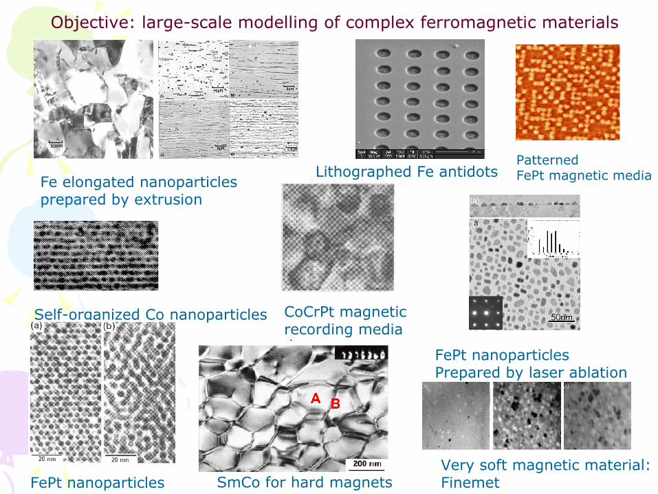
Fe elongated nanoparticles prepared by extrusion

Lithographed Fe antidots

Self-organized Co nanoparticles

FePt nanoparticlesPrepared by laser ablation

CoCrPt magneticrecording media

FePt nanoparticles

Objective: large-scale modelling of complex ferromagnetic materials

SmCo for hard magnetsVery soft magnetic material:Finemet

3.0µm

PatternedFePt magnetic media

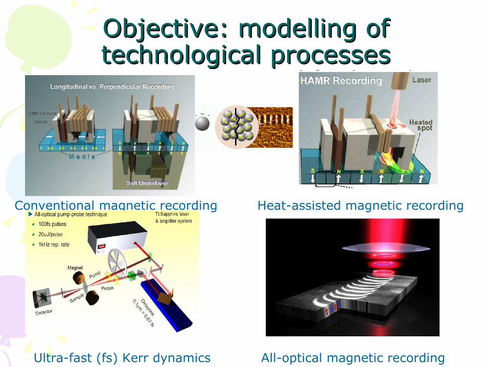
Objective: modelling of Objective: modelling of technological processestechnological processes

Conventional magnetic recording

Ultra-fast (fs) Kerr dynamics

Heat-assisted magnetic recording

All-optical magnetic recording

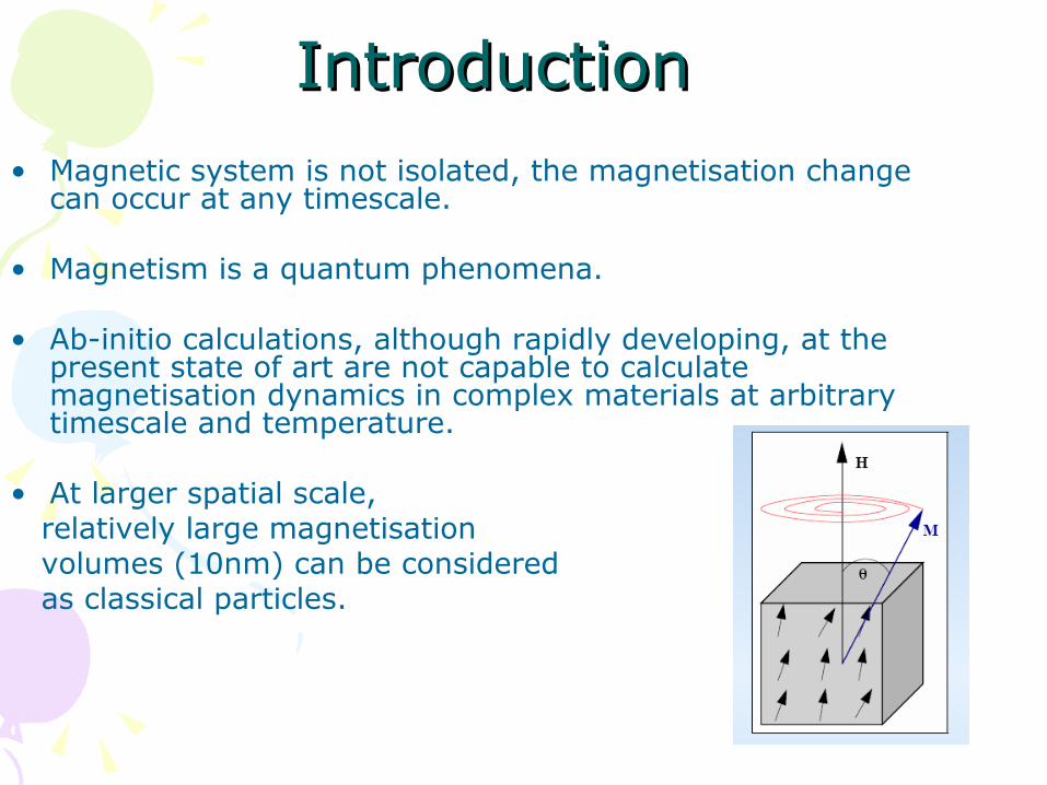
IntroductionIntroduction• Magnetic system is not isolated, the magnetisation change

can occur at any timescale.

• Magnetism is a quantum phenomena.

• Ab-initio calculations, although rapidly developing, at the present state of art are not capable to calculate magnetisation dynamics in complex materials at arbitrary timescale and temperature.

• At larger spatial scale, relatively large magnetisation volumes (10nm) can be considered as classical particles.

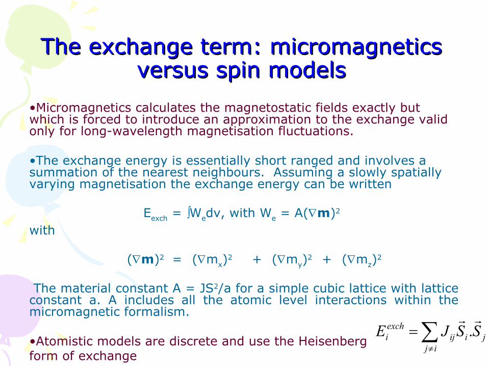
The exchange term: micromagnetics The exchange term: micromagnetics versus spin modelsversus spin models

•Micromagnetics calculates the magnetostatic fields exactly but which is forced to introduce an approximation to the exchange valid only for long-wavelength magnetisation fluctuations.

•The exchange energy is essentially short ranged and involves a summation of the nearest neighbours. Assuming a slowly spatially varying magnetisation the exchange energy can be written

Eexch = Wedv, with We = A(m)2 with 

(m)2 = (mx)2 + (my)2 + (mz)2

 The material constant A = JS2/a for a simple cubic lattice with lattice constant a. A includes all the atomic level interactions within the micromagnetic formalism.

•Atomistic models are discrete and use the Heisenberg form of exchange

jiij

ijexchi SSJE

.

Micromagnetic models of Micromagnetic models of nanostructured materialsnanostructured materials

Models need nanostructure and micromagnetic parameters from experiment

Natural Natural magnetisation magnetisation

dynamics:dynamics:100 pico- 100 100 pico- 100 nano-second nano-second

timescaletimescale

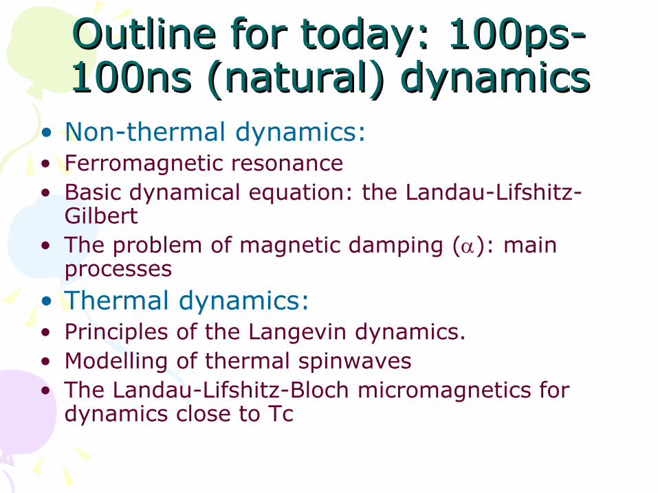
Outline for today: 100ps-Outline for today: 100ps-100ns (natural) dynamics100ns (natural) dynamics

• Non-thermal dynamics:• Ferromagnetic resonance• Basic dynamical equation: the Landau-Lifshitz-

Gilbert• The problem of magnetic damping (): main

processes• Thermal dynamics:• Principles of the Langevin dynamics.• Modelling of thermal spinwaves • The Landau-Lifshitz-Bloch micromagnetics for

dynamics close to Tc

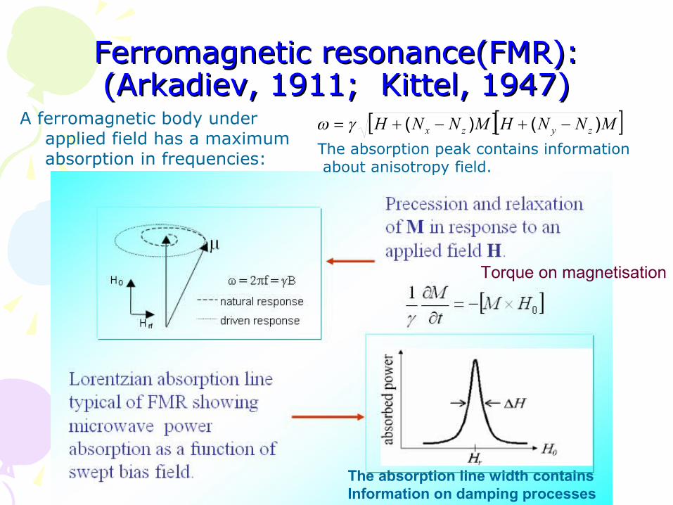
Ferromagnetic resonance(FMR):Ferromagnetic resonance(FMR):(Arkadiev, 1911; Kittel, 1947)(Arkadiev, 1911; Kittel, 1947)

MNNHMNNH zyzx )()(

Torque on magnetisation

The absorption line width contains Information on damping processes

A ferromagnetic body under applied field has a maximum absorption in frequencies:

The absorption peak contains information about anisotropy field.

Ferromagnetic resonanceFerromagnetic resonance• The experiment is normally

performed in almost saturated conditions.

• The absorption peak contains information about anisotropy field.

• The linewidth contains information about dissipation processes.

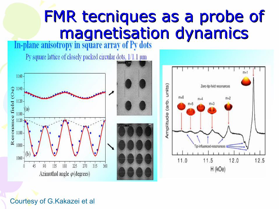
FMR tecniques as a probe of FMR tecniques as a probe of magnetisation dynamicsmagnetisation dynamics

Courtesy of G.Kakazei et al

The Landau-Lifshitz (LL) and the The Landau-Lifshitz (LL) and the Landau-Lifshitz-Gilbert (LLG) equations Landau-Lifshitz-Gilbert (LLG) equations

of motionof motion

HMMM

HMdtMd

s

LL

'

' 00

Landau-Lifshitz damping, 1935

dtMdM

MHM

dtMd

s

G

0

Gilbert damping, 1955

LL equation

Gilbert equation(physically more reasonablefor large damping)

How the Gilbert equation could be transformed into the LL equation

220

0 11 G

GLLG

G

,'

LLG equation

2

0

0 s

s

G

M

MMdtMd

dtMdMM

dtMdMM

MHMM

dtMdM

The LL eq. is equivalent to G equation

with substitutions

(for magnetization vector):

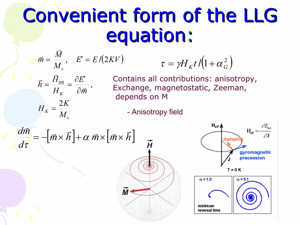
Convenient form of the LLG Convenient form of the LLG equationequation::

sK

K

s

MKH

mE

HHh

KVEEMMm

2

2

,

/,

int

- Anisotropy field

21 GK tH /

hmmhmdmd

Contains all contributions: anisotropy, Exchange, magnetostatic, Zeeman, depends on M

The Bloch-Bloembinger The Bloch-Bloembinger damping:damping:

YXYXYX

MT

HMdtMd

,,, 2

01

)( ZsZZ

MMT

HMdtMd

10

1

Transverse relaxation

Longitudinal relaxation

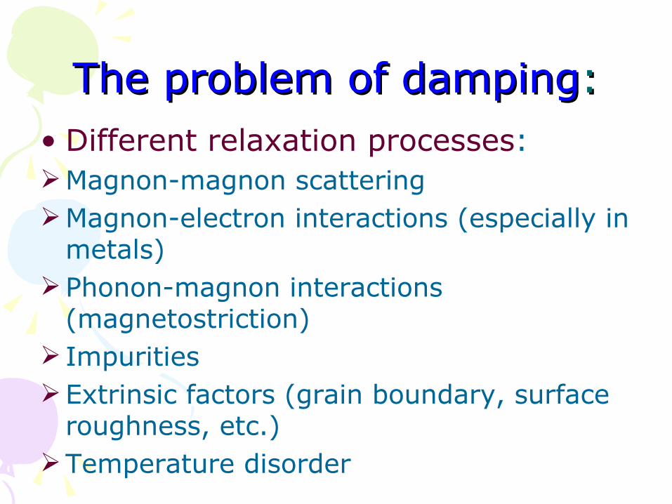
The problem of dampingThe problem of damping::• Different relaxation processes:Magnon-magnon scatteringMagnon-electron interactions (especially in

metals)Phonon-magnon interactions

(magnetostriction) Impurities Extrinsic factors (grain boundary, surface

roughness, etc.)Temperature disorder

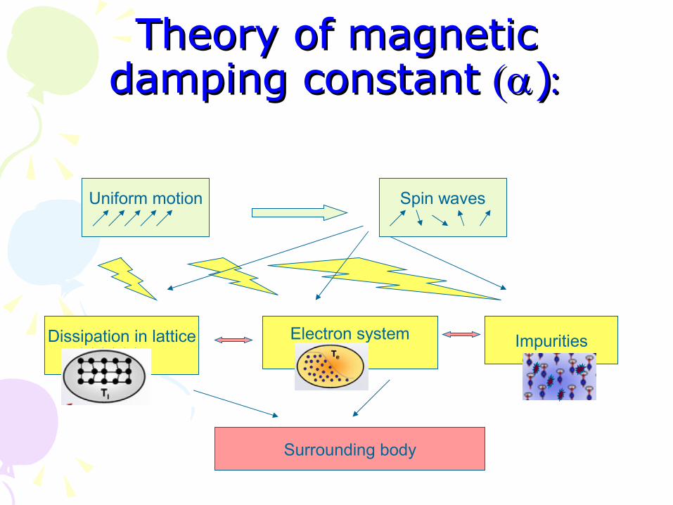
Theory of magnetic Theory of magnetic damping constant damping constant ))

Uniform motion Spin waves

Electron systemDissipation in lattice Impurities

Surrounding body

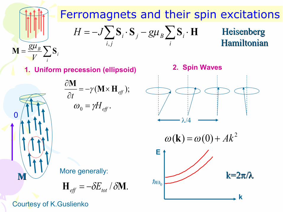
Ferromagnets and their spin excitations

1. Uniform precession (ellipsoid)

i

iBji

ji gJH HSSS ,

H0

);( efftHMM

H

eff

includes:1) Static applied field2) Demagnetization field3) Anisotropy field4) Exchange field

.0 effH

./ MH toteff E

More generally:

2. Spin Waves

2)0()( Ak k

E

k

MM k=2k=2//

HeisenbergHeisenberg HamiltonianHamiltonian

i

iB

Vg SM

Courtesy of K.Guslienko

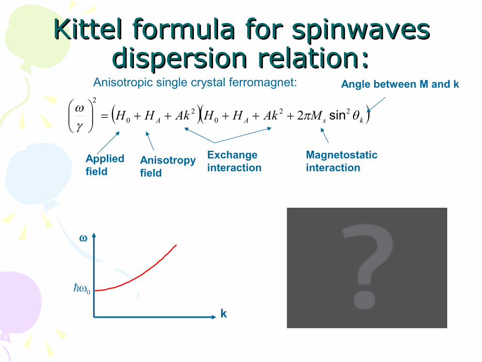
Kittel formula for spinwaves Kittel formula for spinwaves dispersion relation:dispersion relation:

ksAA MAkHHAkHH 22

02

0

2

2 sin

Appliedfield

Anisotropyfield

Exchangeinteraction

Magnetostaticinteraction

Anisotropic single crystal ferromagnet: Angle between M and k

k

Magnons and their Magnons and their interactions:interactions:

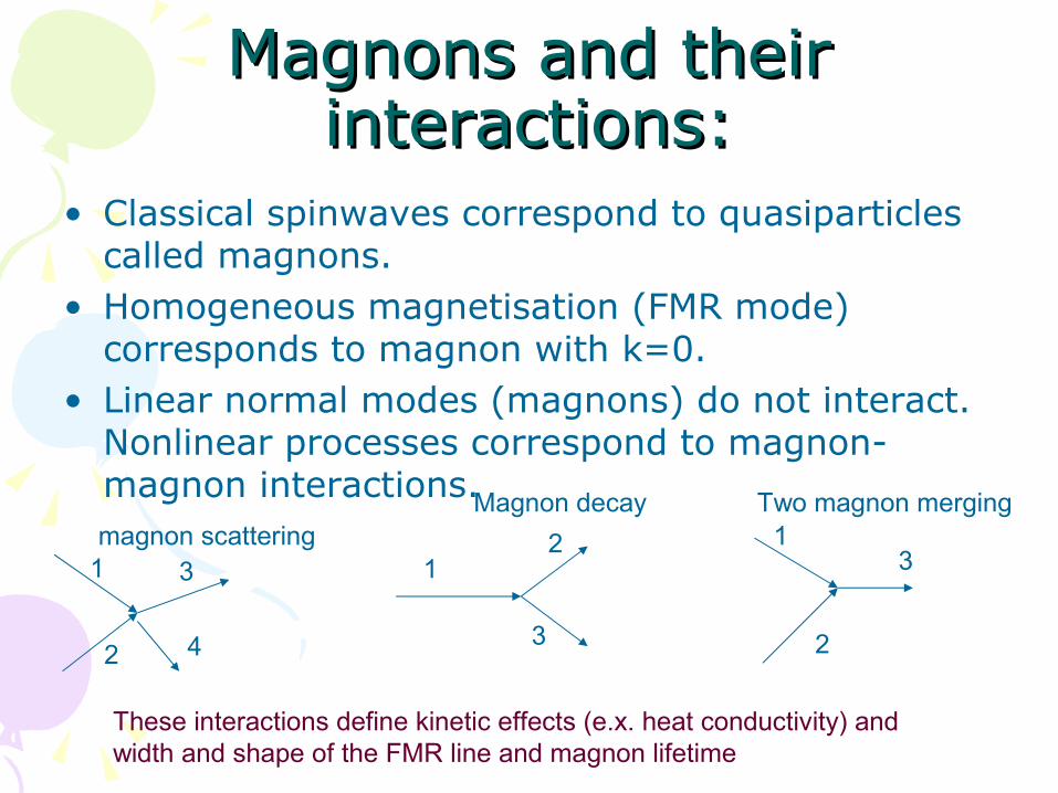
• Classical spinwaves correspond to quasiparticles called magnons.

• Homogeneous magnetisation (FMR mode) corresponds to magnon with k=0.

• Linear normal modes (magnons) do not interact. Nonlinear processes correspond to magnon-magnon interactions.

1

2

3

4

magnon scatteringMagnon decay

12

3

31

2

Two magnon merging

These interactions define kinetic effects (e.x. heat conductivity) andwidth and shape of the FMR line and magnon lifetime

Nonlinear phenomena: Suhl Nonlinear phenomena: Suhl instabilities.instabilities.

• For large excitation power - FMR saturation occurs

• If the density of magnons gets higher than critical value – the homogeneous oscillations become unstable

)()()( kkk 22 0

k=0k

-k

The occurrence of the instability depends on the system geometry and is governed by the applied field.

)()()( kkk 20

Second condition,more easy to meet

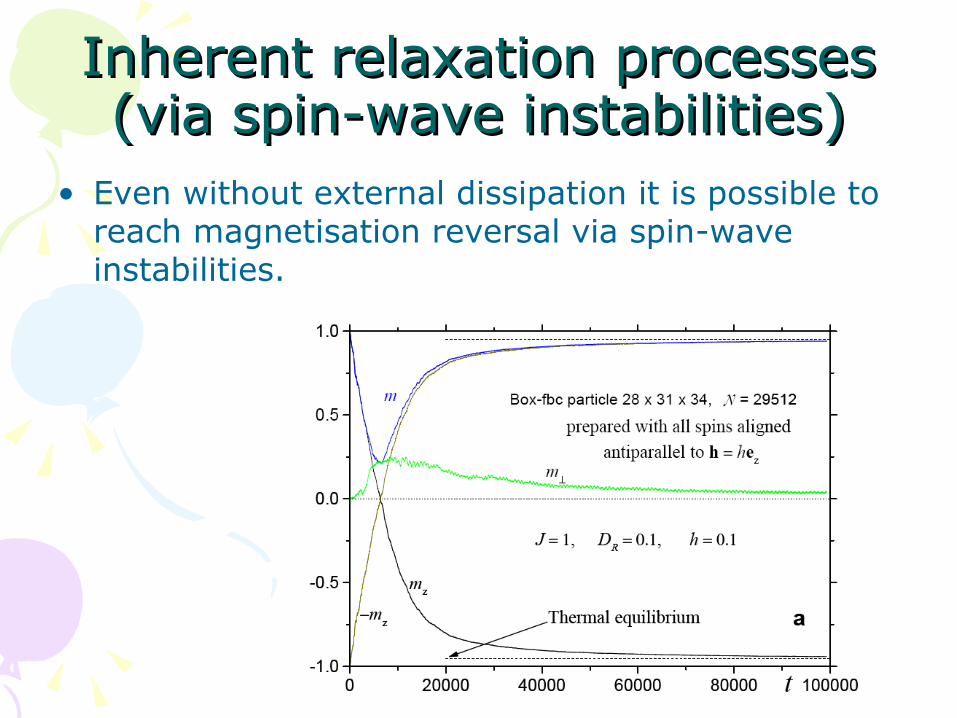
Inherent relaxation processesInherent relaxation processes(via spin-wave instabilities)(via spin-wave instabilities)

• Even without external dissipation it is possible to reach magnetisation reversal via spin-wave instabilities.

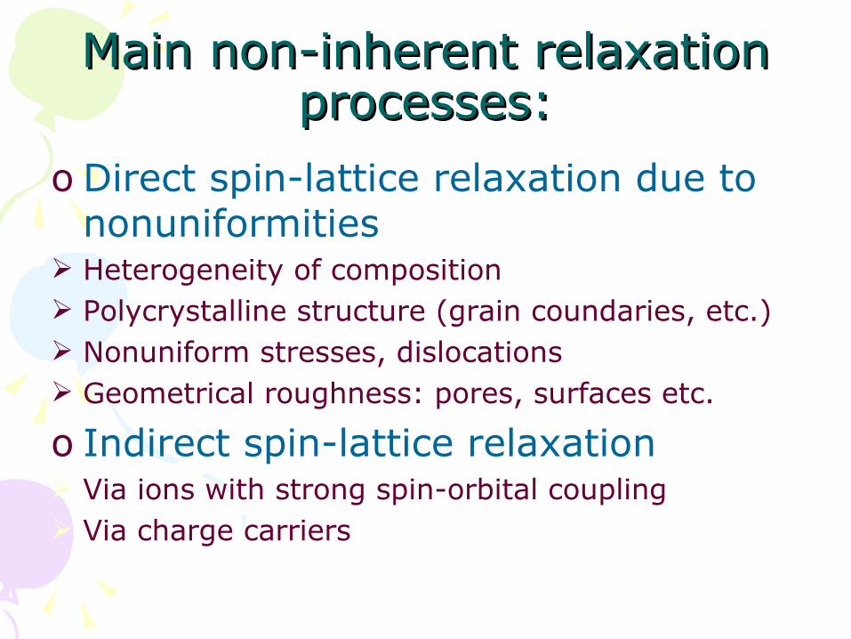
Main non-inherent relaxation Main non-inherent relaxation processes:processes:

o Direct spin-lattice relaxation due to nonuniformities

Heterogeneity of composition Polycrystalline structure (grain coundaries, etc.) Nonuniform stresses, dislocations Geometrical roughness: pores, surfaces etc.

o Indirect spin-lattice relaxation Via ions with strong spin-orbital coupling Via charge carriers

The problem of damping (The problem of damping ())• Although there exist theories trying to

evaluate the damping parameter basing on a particular mechanism, the comparison with experiment remains poor.

• Normally the Gilbert damping is a phenomenological parameter, taken from the experiment.

• The values from FMR and direct measurement of magnetisation switching (fast Kerr measurements) not always coincide.

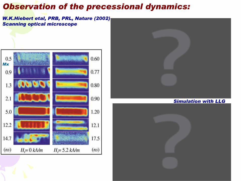
W.K.Hiebert etal, PRB, PRL, Nature (2002)Scanning optical microscope

Observation of the precessional dynamics:

Simulation with LLG

Mx

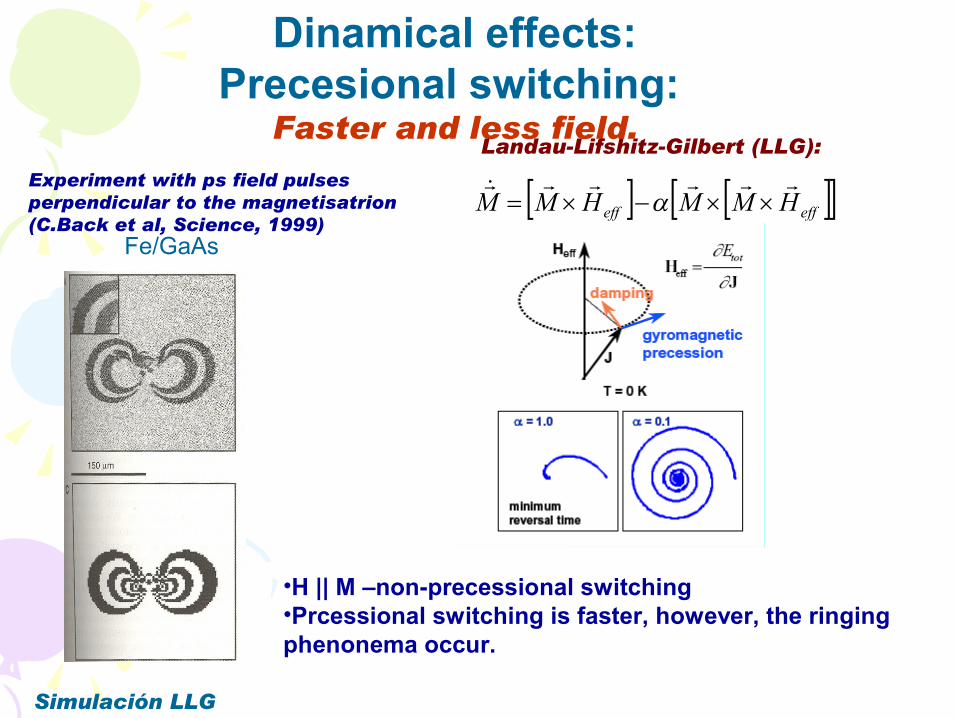
Dinamical effects:Precesional switching:

Faster and less field.

Experiment with ps field pulses perpendicular to the magnetisatrion(C.Back et al, Science, 1999)

Simulación LLG

Landau-Lifshitz-Gilbert (LLG):

effeff HMMHMM

•H || M –non-precessional switching•Prcessional switching is faster, however, the ringingphenonema occur.

Fe/GaAs

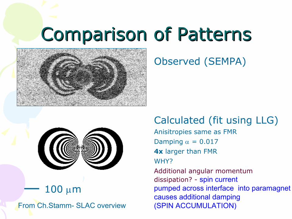
Comparison of Comparison of PatternsPatternsObserved (SEMPA)

Calculated (fit using LLG)Anisitropies same as FMR

Damping = 0.0174x larger than FMR

WHY?Additional angular momentumdissipation? - spin current pumped across interface into paramagnetcauses additional damping (SPIN ACCUMULATION)

100 m

From Ch.Stamm- SLAC overview

Thermal effectsThermal effects

Thermal fluctuations play very important Thermal fluctuations play very important role in magnetisation dynamics:role in magnetisation dynamics:

At the microscopic level:• At the equilibrium they are responsible for thermally

excited spinwaves.• Spinwaves are responsible for thermal magnetisation

reversal via the spinwave instabilities and energy transfer to main reversal mode.

At more macroscopic level•Thermal fluctuations are responsible for random walk in a complex energy landscape•Eventually energy barriers could be overcome with the help of thermal fluctuations leading to magnetisation decay.

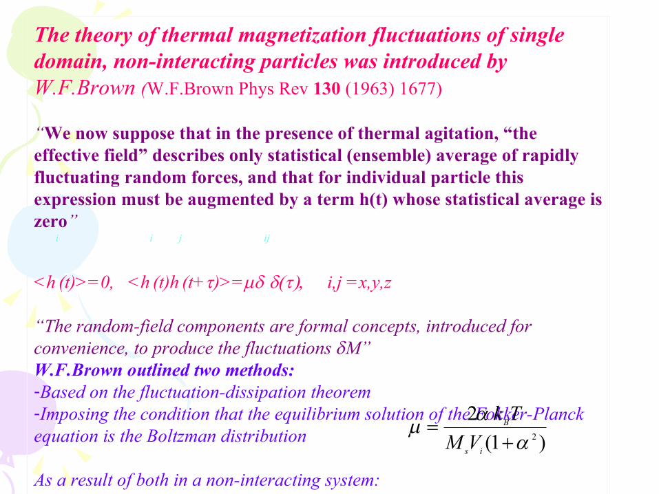
The theory of thermal magnetization fluctuations of single domain, non-interacting particles was introduced by W.F.Brown (W.F.Brown Phys Rev 130 (1963) 1677)

“We now suppose that in the presence of thermal agitation, “the effective field” describes only statistical (ensemble) average of rapidly fluctuating random forces, and that for individual particle this expression must be augmented by a term h(t) whose statistical average is zero”

<h

i

(t)>=0, <h

i

(t)h

j

(t+)>=

ij

i,j =x,y,z

“The random-field components are formal concepts, introduced for convenience, to produce the fluctuations M”W.F.Brown outlined two methods:-Based on the fluctuation-dissipation theorem-Imposing the condition that the equilibrium solution of the Fokker-Planck equation is the Boltzman distribution

As a result of both in a non-interacting system:

)1(2

2

is

B

VMTk

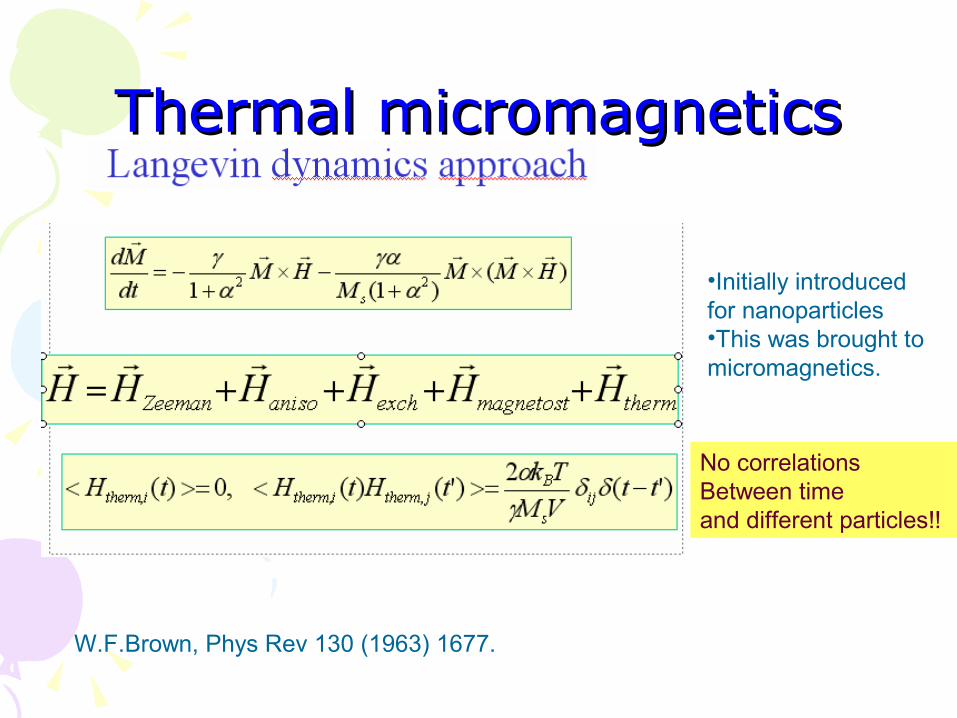
Thermal micromagneticsThermal micromagnetics

W.F.Brown, Phys Rev 130 (1963) 1677.

•Initially introducedfor nanoparticles•This was brought tomicromagnetics.

No correlationsBetween timeand different particles!!

Note on the damping and Note on the damping and thermal processes.thermal processes.

• In principle, the Gilbert (or other) form of damping is as a result of spin coupling with the oscillator thermal bath, in this sense, the thermal fluctuations are already included into the damping term.

• In some approximations, the undamped LL equation is coupled to a system of oscillators (phenomenological phonon bath) and the resulting LLG damping is derived.

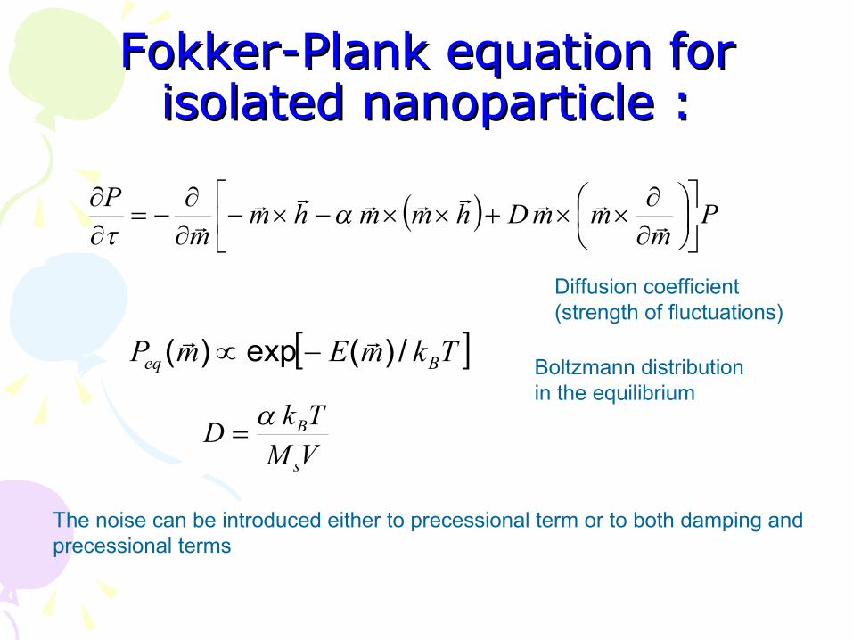
Fokker-Plank equation for Fokker-Plank equation for isolated nanoparticle :isolated nanoparticle :

Pm

mmDhmmhmm

P

TkmEmP Beq /)(exp)(

Diffusion coefficient(strength of fluctuations)

VMTkD

s

B

Boltzmann distributionin the equilibrium

The noise can be introduced either to precessional term or to both damping andprecessional terms

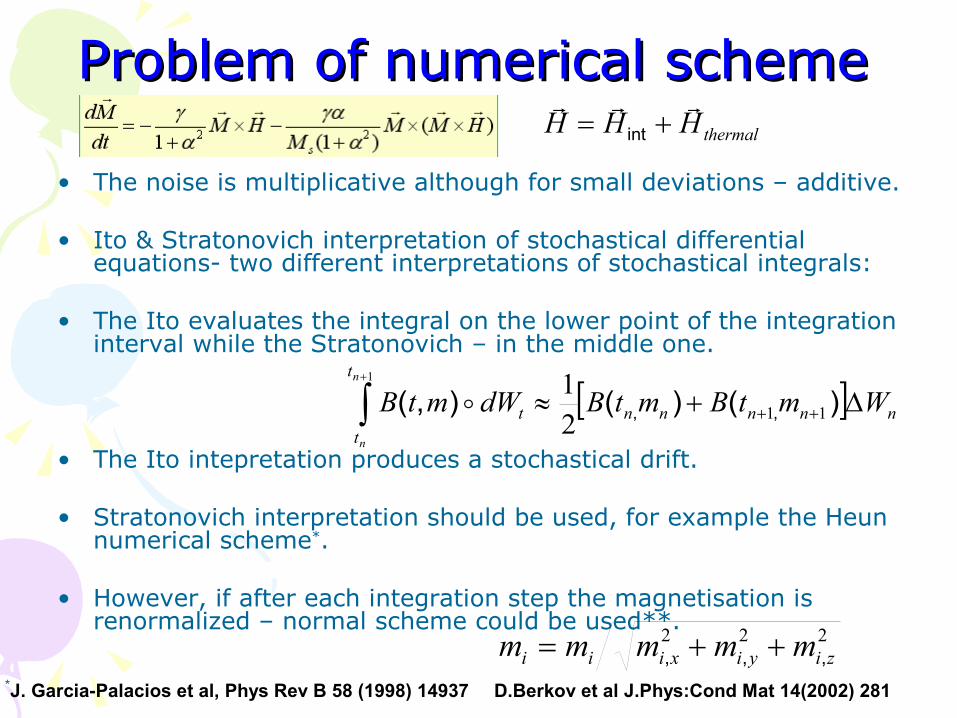
Problem of numerical schemeProblem of numerical scheme

• The noise is multiplicative although for small deviations – additive.

• Ito & Stratonovich interpretation of stochastical differential equations- two different interpretations of stochastical integrals:

• The Ito evaluates the integral on the lower point of the integration interval while the Stratonovich – in the middle one.

• The Ito intepretation produces a stochastical drift.

• Stratonovich interpretation should be used, for example the Heun numerical scheme*.

• However, if after each integration step the magnetisation is renormalized – normal scheme could be used**. 222

ziyixiii mmmmm ,,,

nnnnn

t

tt WmtBmtBdWmtB

n

n

)()(),( ,, 11

1

21

*J. Garcia-Palacios et al, Phys Rev B 58 (1998) 14937 **D.Berkov et al J.Phys:Cond Mat 14(2002) 281

thermalHHH

int

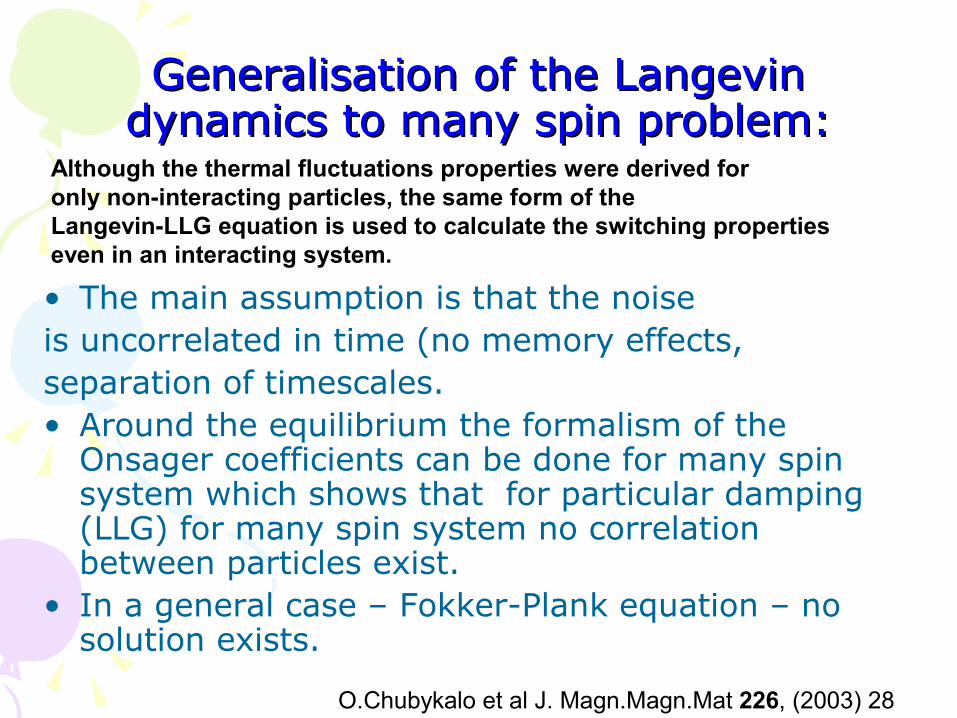
Generalisation of the Langevin Generalisation of the Langevin dynamics to many spin problem:dynamics to many spin problem:

• The main assumption is that the noiseis uncorrelated in time (no memory effects,separation of timescales.• Around the equilibrium the formalism of the

Onsager coefficients can be done for many spin system which shows that for particular damping (LLG) for many spin system no correlation between particles exist.

• In a general case – Fokker-Plank equation – no solution exists.

Although the thermal fluctuations properties were derived for only non-interacting particles, the same form of the Langevin-LLG equation is used to calculate the switching properties even in an interacting system.

O.Chubykalo et al J. Magn.Magn.Mat 226, (2003) 28

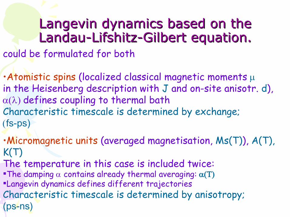
Langevin dynamics based on the Langevin dynamics based on the Landau-Lifshitz-Gilbert equation.Landau-Lifshitz-Gilbert equation.

could be formulated for both

•Atomistic spins (localized classical magnetic moments in the Heisenberg description with J and on-site anisotr. d), defines coupling to thermal bathCharacteristic timescale is determined by exchange;fs-ps)

•Micromagnetic units (averaged magnetisation, Ms(T)), A(T), K(T) The temperature in this case is included twice:The damping contains already thermal averaging: Langevin dynamics defines different trajectoriesCharacteristic timescale is determined by anisotropy; (ps-ns)

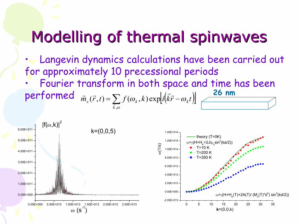
Modelling of thermal spinwavesModelling of thermal spinwaves• Langevin dynamics calculations have been carried outfor approximately 10 precessional periods• Fourier transform in both space and time has beenperformed 26 nm

0.00E+000 5.00E+012 1.00E+013 1.50E+013 2.00E+013 2.50E+013

0.00E+000

1.00E+011

2.00E+011

3.00E+011

4.00E+011

5.00E+011

6.00E+011 k=(0,0,5) |f(,k)|2

(s-1)

,

exp),(),(k

kkx trkikftrm

0 5 10 15 20 25 30 35-2.00E+013

0.00E+000

2.00E+013

4.00E+013

6.00E+013

8.00E+013

1.00E+014

1.20E+014

1.40E+014

=(H+HK(T)+2A(T)/ (Ms(T)*d2) sin2(kd/2))

(1

/s)

k=(0,0,k)

theory (T=0K)=(H+H

K+2J/

ssin2(ka/2))

T=10 K T=200 K T=350 K

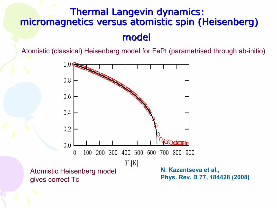
Thermal Langevin dynamics: Thermal Langevin dynamics: micromagnetics versus atomistic spin (Heisenberg) micromagnetics versus atomistic spin (Heisenberg)

modelmodel

Atomistic Heisenberg modelgives correct Tc

Atomistic (classical) Heisenberg model for FePt (parametrised through ab-initio)

N. Kazantseva et al., Phys. Rev. B 77, 184428 (2008)

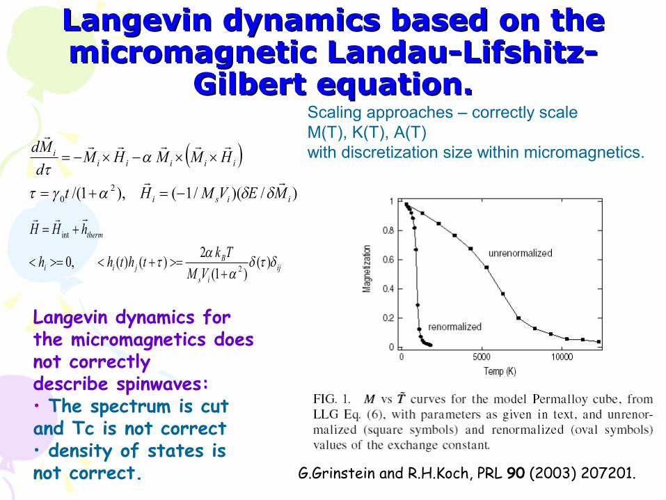
Langevin dynamics based on the Langevin dynamics based on the micromagnetic Landau-Lifshitz-micromagnetic Landau-Lifshitz-

Gilbert equation.Gilbert equation.

)/)(/1(),1/( 2

0 iisi

iiiiii

MEVMHt

HMMHMdMd

ijis

Bjii

therm

VMTkththh

hHH

)(

)1(2)()(,0 2

int

G.Grinstein and R.H.Koch, PRL 90 (2003) 207201.

Langevin dynamics for the micromagnetics does not correctlydescribe spinwaves:• The spectrum is cut and Tc is not correct• density of states is not correct.

Scaling approaches – correctly scale M(T), K(T), A(T) with discretization size within micromagnetics.

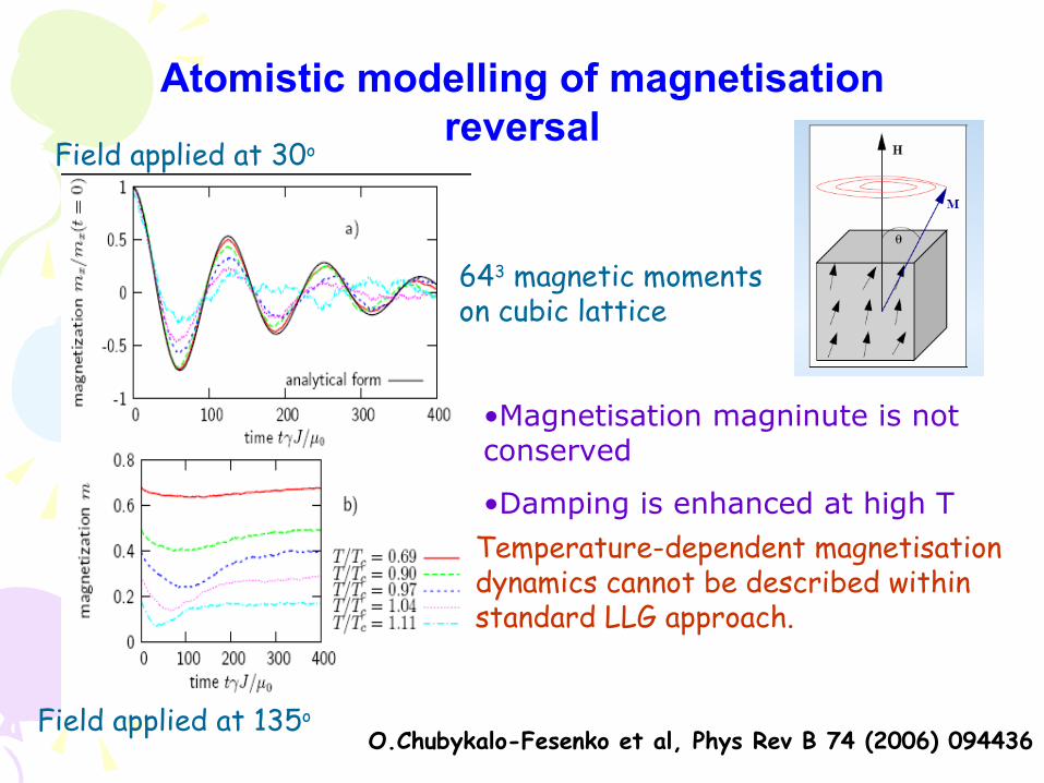
Atomistic modelling of magnetisation reversal

643 magnetic momentson cubic lattice

Field applied at 30o

Field applied at 135o

•Magnetisation magninute is not conserved

•Damping is enhanced at high T

Temperature-dependent magnetisationdynamics cannot be described withinstandard LLG approach.

O.Chubykalo-Fesenko et al, Phys Rev B 74 (2006) 094436

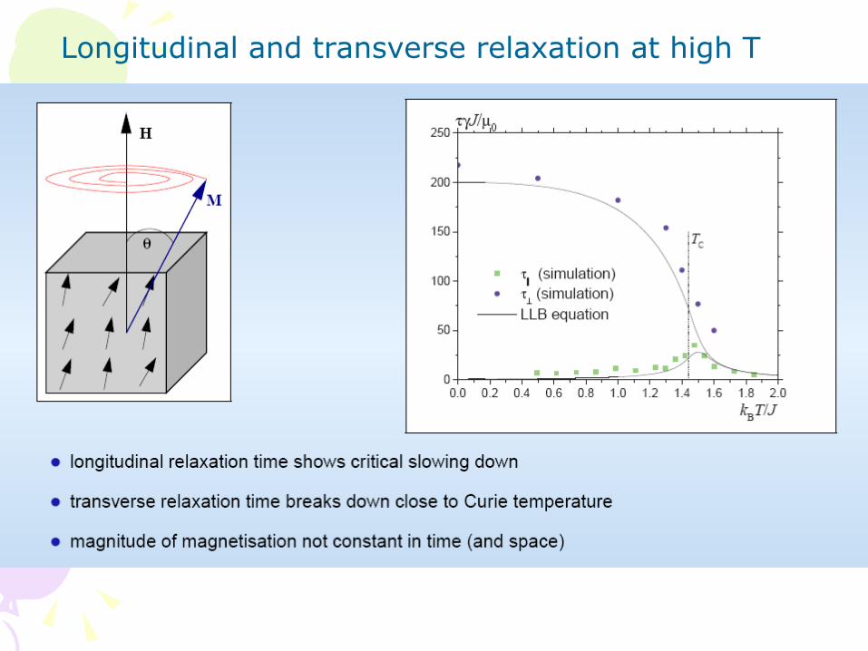
Longitudinal and transverse relaxation at high T

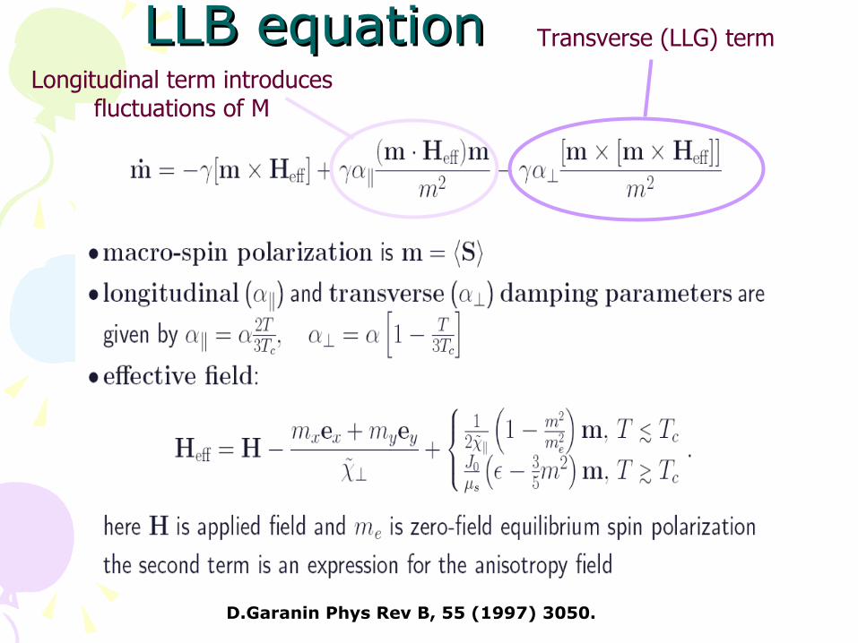
LLB equationLLB equation Transverse (LLG) term

Longitudinal term introduces fluctuations of M

D.Garanin Phys Rev B, 55 (1997) 3050.

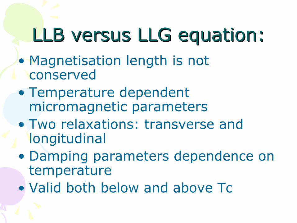
LLB versus LLG equation:LLB versus LLG equation:• Magnetisation length is not

conserved• Temperature dependent

micromagnetic parameters• Two relaxations: transverse and

longitudinal• Damping parameters dependence on

temperature• Valid both below and above Tc

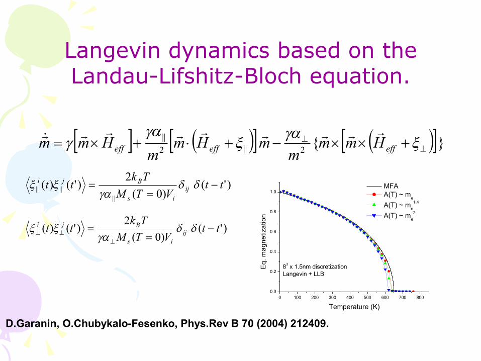
Langevin dynamics based on theLandau-Lifshitz-Bloch equation.

}{2||2||

effeffeff Hmm

mmHm

mHmm

)'()0(

2)'()(

|||||| tt

VTMTktt ij

is

Bji

)'()0(

2)'()( tt

VTMTktt ij

is

Bji

D.Garanin, O.Chubykalo-Fesenko, Phys.Rev B 70 (2004) 212409.

0 100 200 300 400 500 600 700 8000.0

0.2

0.4

0.6

0.8

1.0

83 x 1.5nm discretizationLangevin + LLB

Eq.

mag

netiz

atio

n

Temperature (K)

MFA A(T) ~ me

A(T) ~ me1.4

A(T) ~ me2

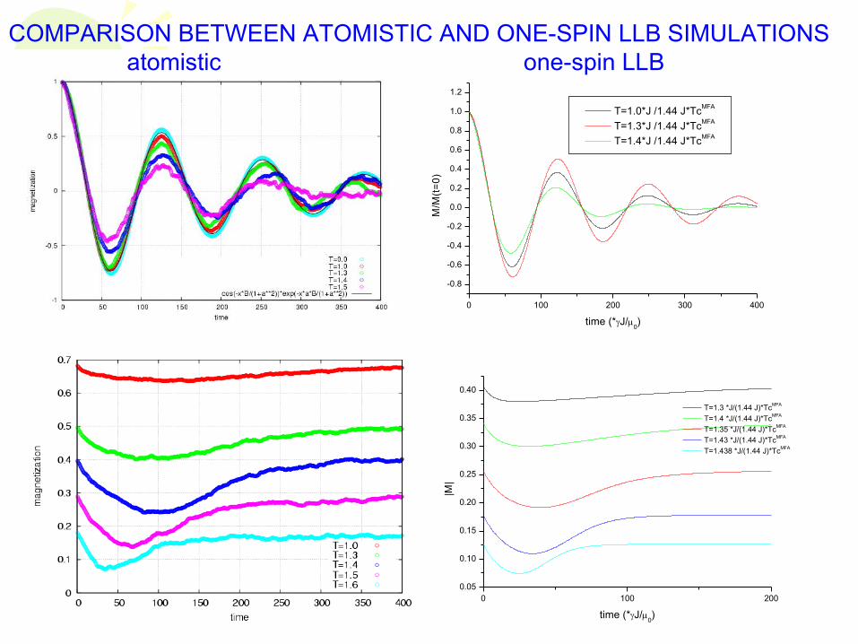
0 100 2000.05

0.10

0.15

0.20

0.25

0.30

0.35

0.40

|M|

time (*J/0)

T=1.3 *J/(1.44 J)*TcMFA

T=1.4 *J/(1.44 J)*TcMFA

T=1.35 *J/(1.44 J)*TcMFA

T=1.43 *J/(1.44 J)*TcMFA

T=1.438 *J/(1.44 J)*TcMFA

0 100 200 300 400

-0.8

-0.6

-0.4

-0.2

0.0

0.2

0.4

0.6

0.8

1.0

1.2

M/M

(t=0)

time (*J/0)

T=1.0*J /1.44 J*TcMFA

T=1.3*J /1.44 J*TcMFA

T=1.4*J /1.44 J*TcMFA

COMPARISON BETWEEN ATOMISTIC AND ONE-SPIN LLB SIMULATIONS atomistic one-spin LLB

Multscale approachMultscale approach

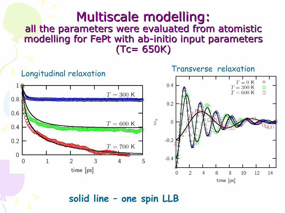
Multiscale modelling:Multiscale modelling:all the parameters were evaluated from atomistic all the parameters were evaluated from atomistic modelling for FePt with ab-initio input parameters modelling for FePt with ab-initio input parameters

(Tc= 650K)(Tc= 650K)

solid line – one spin LLB

Longitudinal relaxation Transverse relaxation

• The usual formalism for large-scale calculations of magnetic properties is Micromagnetics.

• Although different theories of magnetic damping parameters exist, due to a complexity of the problem, the damping parameter remains phenomenological.

• Thermal effects can be introduced, but the limitation of long-wavelength fluctuations means that the standard micromagnetics cannot reproduce phase transitions.

• The Landau-Lifshitz-Bloch equation is a valid micromagnetic formalism for high temperatures.

CONCLUSIONS