Chaotic Behaviour of the Magnetic Pendulum

Christopher J. Lang20557510

December 4, 2015

Abstract

Magnetic pendulums are a simple, real-world example of chaos. Many other studiesexamine the chaotic behaviour of magnetic pendulums; however, this report extendsthe discussion by considering the effects of differing levels of attraction and repulsionon this chaotic behaviour. This paper first rigorously derives the initial value problemthat approximately describes the motion of a magnetic pendulum, based on explicitassumptions made about the model. This paper then discusses the two-fold chaoticbehaviour of that motion.

Contents

1 Introduction . . . . . . . . . . . . . . . . . . . . . . . . . . . . . . . . . . . . . . 21.1 Terminology . . . . . . . . . . . . . . . . . . . . . . . . . . . . . . . . . . . . 21.2 Assumptions . . . . . . . . . . . . . . . . . . . . . . . . . . . . . . . . . . . . 21.3 Symbols . . . . . . . . . . . . . . . . . . . . . . . . . . . . . . . . . . . . . . 3

2 Equations . . . . . . . . . . . . . . . . . . . . . . . . . . . . . . . . . . . . . . . 4

3 Analysis . . . . . . . . . . . . . . . . . . . . . . . . . . . . . . . . . . . . . . . . 4

4 Numeric Solutions . . . . . . . . . . . . . . . . . . . . . . . . . . . . . . . . . . 8

5 Conclusions . . . . . . . . . . . . . . . . . . . . . . . . . . . . . . . . . . . . . . 10

6 Appendix: Figures . . . . . . . . . . . . . . . . . . . . . . . . . . . . . . . . . . 12

1

1 Introduction

The following subsections outline the terminology, assumptions, and symbols used in thereport.

1.1 Terminology

The following terms are used throughout this report:

1: Chaos is a difficult concept to define mathematically. Many chaos scientists and text-books cannot agree on a single definition of chaos [4]. In this report we use Lorenz’sdefinition:

Chaos: When the present determines the future, but the approximatepresent does not approximately determine the future [1].

In other words, chaos is the sensitivity of a system to initial conditions.

2: A magnetic pendulum is quite similar to the simple pendulum; however, there are afew alterations. In this paper, we use the following definition:

Magnetic Pendulum: A pendulum with a magnet acting as a bob, whichis attracted or repelled by magnets lying on a plane unreachable by thependulum .

1.2 Assumptions

The following assumptions are used in this model:

1: The observations are made in an inertial reference frame.

2: The pendulum is centred on the origin of the xy-plane of a Cartesian coordinate system,where height is measured upwards.

3: The pendulum is anchored such that the pendulum lies above the xy-plane, the planeupon which the other magnets are placed.

4: The length of the pendulum is constant.

5: The minimum height of the bob is much less than the length of the pendulum.

6: The magnets are point attractors.

7: The spacing of the magnets is much smaller than the length of the pendulum.

8: The pendulum does not travel far from the magnets.

9: The pendulum starts from rest.

2

10: The magnitude of the magnetic force between two point attractors is inversely pro-portional to the square of the distance between them. Furthermore, it points in thedirection of the relative position of the magnet with respect to the bob.

11: The drag force that acts on the pendulum bob is linearly proportional to its velocityand opposes motion.

1.3 Symbols

The following table outlines the various symbols used throughout the report. Note thata boldface symbol is a vector. Also, a dot above a symbol indicates taking the derivativewith respect to time. Furthermore, a symbol between { and } indicates a set, whose upperand lower bounds are represented by superscripts and upperscripts after the }, respectively.Finally, note that the table is in alphabetical order, with greek letters appearing alphabeti-cally after latin letters.

Symbol Description

bProportionality constant fordrag force.

F Net force on the pendulum.

FdDrag force on the pendulumbob.

FgForce of gravity on the pendu-lum bob.

{Fmi}ni=1

Magnetic force on the pendulumbob by each magnet.

gThe magnitude of the accelera-tion due to gravity.

hThe minimum height of the pen-dulum above the plane.

iIndex for the magnets on theplane.

k Unit vector for the z-axis.

{ki}ni=1Proportionality constant foreach magnetic force.

L The length of the pendulum.

m Mass of the pendulum bob.

nThe number of magnets on theplane.

P The ratio of b to m.

Symbol Description

Q The ratio of g to L.

r Position of the pendulum bob.

{Ri}ni=1 The ratio of each ki to m.

TTension force on the pendulumbob.

Txx-coordinate of the tensionforce.

Ty y-coordinate of the tension force.

Tz z-coordinate of the tension force.

xx-coordinate of the position ofthe pendulum bob.

x0x-coordinate of the initial posi-tion.

yy-coordinate of the position ofthe pendulum bob.

y0y-coordinate of the initial posi-tion.

zz-coordinate of the position ofthe pendulum bob.

θAzimuthal angle of the tensionforce.

φInclination angle of the tensionforce.

3

2 Equations

In this section we will derive and review some of the equations that will be used in de-riving the initial value problem.

As we are in an intertial reference frame (assumption 1), from Newton’s Second Law wehave: ∑

F = mr

As the forces that act on the pendulum bob are: Fg, Fd, T, and {Fmi}ni=1,

Fg + Fd + T +n∑

i=1

Fmi= mr (2.1)

From assumption 11 we have that Fd ∝ r. As the drag force opposes motion, let b ∈ R,b > 0, such that,

Fd = −br (2.2)

Let i ∈ N, i ≤ n. Also, let r′i := ri − r. As we are dealing with point attractors,assumption 6, we have that Fmi

∝ 1

‖r′i‖2 r′i, from assumption 10. Let ki ∈ R such that,

Fmi=

ki

‖r′i‖2 r′i

As r′i =r′i

‖r′i‖,

Fmi=

ki

‖r′i‖3 r′i (2.3)

3 Analysis

In this section we will derive the simplified initial value problem that approximately de-scribes the behaviour of the magnetic pendulum, given our assumptions.

From assumption 4 we have that L is constant. Let h be the minimum height of thependulum. As the pendulum is centred on the origin of the xy-plane of a Cartesian coordinatesystem, assumption 2, for a given r = (x, y, z) we have that the position of the bob, relativeto the anchor, is: (x, y, z − L− h). As the length of the pendulum is L,

x2 + y2 + (z − L− h)2 = L2

Solving for z,

z = L+ h±√L2 − x2 − y2

4

As the pendulum bob is close to the magnets, assumption 8, we must reject the plusoption in the above ±. Thus,

z = L+ h−√L2 − x2 − y2 (3.1)

From assumption 8 we have that the pendulum does not travel far from the magnets.Furthermore, from assumption 7 we have that the spacing of the magnets is much less thatlength of the pendulum. Thus, x and y are much smaller than L.

Expanding√L2 − x2 − y2 using the Maclaurin series,√

L2 − x2 − y2 =√L2 − 02 − 02 − x2

2√L2 − 02 − 02

− y2

2√L2 − 02 − 02

+ . . .

As x and y are small compared with L, we ignore the quadratic and higher degree terms,leaving: √

L2 − x2 − y2 ≈ L

Therefore,

z ≈ h (3.2)

Thus, z ≈ 0 and z ≈ 0, as z is approximately constant.

As Fg = −mgk, consider the z-component of (2.1), substituting (2.2) and (2.3),

−mg − bz + Tz +n∑

i=1

ki(√(xi − x)2 + (yi − y)2 + (zi − z)2

)3 (zi − z) = mz

From assumption 3 we have that the magnets all lie on the xy-plane. Thus, zi = 0,∀i ∈ N, i ≤ n. As z ≈ h, z ≈ 0, and z ≈ 0,

−mg + Tz − hn∑

i=1

ki(√(xi − x)2 + (yi − y)2 + h2

)3 = 0

Solving for Tz,

Tz = mg + h

n∑i=1

ki(√(xi − x)2 + (yi − y)2 + h2

)3As Tz = ‖T‖ cosφ, we get

‖T‖ cosφ = mg + hn∑

i=1

ki(√(xi − x)2 + (yi − y)2 + h2

)3 (3.3)

Solving (3.1) for L+ h− z, we get

5

L+ h− z =√L2 − x2 − y2 (3.4)

As cosφ = L+h−zL

, substituting (3.4),

cosφ =

√L2 − x2 − y2

L

Substituting into (3.3) and solving for ‖T‖,

‖T‖ =mgL√

L2 − x2 − y2+

hL√L2 − x2 − y2

n∑i=1

ki(√(xi − x)2 + (yi − y)2 + h2

)3 (3.5)

As Tx = −‖T‖ sinφ cos θ,

Tx = − sinφ cos θ

mgL√L2 − x2 − y2

+hL√

L2 − x2 − y2

n∑i=1

ki(√(xi − x)2 + (yi − y)2 + h2

)3

(3.6)

As cosφ =

√L2−x2−y2

L, it follows that sinφ =

√x2+y2

L, as sinφ ≥ 0, as 0 ≤ φ ≤ π.

Furthermore, cos θ = x√x2+y2

, so sinφ cos θ = xL

. Substituting into (3.6) and simplifying,

Tx = − mgx√L2 − x2 − y2

− hx√L2 − x2 − y2

n∑i=1

ki(√(xi − x)2 + (yi − y)2 + h2

)3As√L2 − x2 − y2 ≈ L,

Tx = −mgxL− hx

L

n∑i=1

ki(√(xi − x)2 + (yi − y)2 + h2

)3From assumption 5, h is small compared with L. As h and x are small compared with

L, we ignore any quadratic terms. Thus,

Tx = −mgLx (3.7)

Similarly, Ty = −‖T‖ sinφ sin θ. As sin θ = y√x2+y2

and sinφ =

√x2+y2

L, it follows that

sinφ sin θ = y√x2+y2

. Thus,

Tx = − mgy√L2 − x2 − y2

− hy√L2 − x2 − y2

n∑i=1

ki(√(xi − x)2 + (yi − y)2 + h2

)36

Using√L2 − x2 − y2 ≈ L and ignoring the quadratic terms,

Ty = −mgLy (3.8)

As z ≈ h, z ≈ 0, and z ≈ 0, we can ignore z. Substituting (2.2), (2.3), (3.7), and (3.8)into (2.1),

−bx− mg

Lx+

n∑i=1

ki(√(xi − x)2 + (yi − y)2 + h2

)3 (xi − x) = mx

−by − mg

Ly +

n∑i=1

ki(√(xi − x)2 + (yi − y)2 + h2

)3 (yi − y) = my

Dividing by m, as m 6= 0, and rearranging,

x+b

mx+

g

Lx+

1

m

n∑i=1

ki(√(xi − x)2 + (yi − y)2 + h2

)3 (x− xi) = 0

y +b

my +

g

Ly +

1

m

n∑i=1

ki(√(xi − x)2 + (yi − y)2 + h2

)3 (y − yi) = 0

Let P := bm

, Q := gL

, and Ri := kim

, ∀i ∈ N, i ≤ n. Then our system is:

x+ Px+Qx+n∑

i=1

Ri(√(xi − x)2 + (yi − y)2 + h2

)3 (x− xi) = 0

y + P y +Qy +n∑

i=1

Ri(√(xi − x)2 + (yi − y)2 + h2

)3 (y − yi) = 0

From assumption 9, any solution to this system must satisfy x(0) = 0 and y(0) = 0.Note that this assumption helps ensure that the system satisfies assumption 8 as it evolves.This is because assumption 9 makes sure the pendulum cannot start by going near the speedof light, for instance, which would certainly make the pendulum travel far away from themagnets. Moreover, any solution to this system must also satisfy x(0) = x0 and y(0) = y0,where x0, y0 ∈ R are small, in order for the system to satisfy assumption 8.

7

Summarizing, our initial value problem is:

x+ Px+Qx+n∑

i=1

Ri(√(xi − x)2 + (yi − y)2 + h2

)3 (x− xi) = 0 (3.9)

y + P y +Qy +n∑

i=1

Ri(√(xi − x)2 + (yi − y)2 + h2

)3 (y − yi) = 0 (3.10)

satisfying: x(0) = 0, y(0) = 0, x(0) = x0, and y(0) = y0.

4 Numeric Solutions

In this section we demonstrate the two-fold chaotic behaviour of the magnetic pendulumthrough graphs calculated using numeric methods.

Table 1 outlines the values of the various parameters of the system for figures 1 through7:

Figure P Q h n {Ri}ni=1 {xi}ni=1 {yi}ni=1

1 0.2 0.1 0.5 2 10, 10 1, -1 0, 0

2 0.2 0.1 0.5 2 20, 10 1, -1 0, 0

3 0.2 0.1 0.5 3 10, 10, 10√32

, −√32

, 0 12, 1

2, -1

4 0.2 0.1 0.5 3 10, 10, -10√32

, −√32

, 0 12, 1

2, -1

5 0.2 0.1 0.5 3 -10, -10, -10√32

, −√32

, 0 12, 1

2, -1

6 0.2 1.0 0.5 3 10, 10, 10√32

, −√32

, 0 12, 1

2, -1

7 2.0 1.0 0.5 3 10, 10, 10√32

, −√32

, 0 12, 1

2, -1

Table 1: Parameter values for chaotic plots

These values for the parameters were chosen to demonstrate the effects that: the numberof magnets, repulsion, differing levels of attraction, drag, and gravity can have on the chaoticbehaviour of the system.

The following figures represent the ending positions of the pendulum based on variousstarting points. Any given pixel represents the initial point and is assigned a colour depend-ing on where it tends towards or away from for high values of t.

8

In figure 1 there are two equally attracting magnets placed at (1, 0) and (−1, 0). It isevident from the figure that the system is quite chaotic when the initial point is far fromthe magnets; however, as the initial point approaches the magnets, this chaotic behaviourdisappears.

In figure 2 there are two attracting magnets placed at (1, 0) and (−1, 0). From table 1we see that the magnet at (1, 0) has twice the level of attraction compared to the magnet at(−1, 0). The figure clearly shows that, while there is still some chaos, the differing levels ofattraction has significantly reduced the chaotic behaviour of the system.

In figure 3 there are three equally attracting magnets placed at (√32, 12), (−

√32, 12), and

(0,−1). This scenario is the same as in 1, except that one magnet has been added. Addi-tionally, the magnets have been shifted to better demonstrate the symmetry of the chaos.When comparing with figure 1, the regions of low chaotic behaviour are smaller; however,once you leave these regions, the behaviour is immediately much more chaotic than the casewith two equally attracting magnets. This shows that increasing the number of magnets hasincreased the level of chaotic behaviour in the system.

Figure 4 is essentially the same scenario as in figure 3; however, the bottom magnet repelsthe pendulum bob. Observe, from table 1, that the magnitude of the repulsion is the sameas the attraction of the other two magnets. It is interesting to note that around the twoattracting magnets, we observe behaviour similar to that of the case of two equally attractingmagnets. Although, around the repelling magnet, we see much more chaotic behaviour thanfor the other magnets; however, not as much chaotic behaviour as in the case of the threeequally attracting magnets.

In figure 5 we essentially have the same scenario as in figure 3; except that the magnetsare now equally repelling the pendulum, not attracting it. Due to the nature of being repelledby all of the magnets, the meaning of the colours has changed for this figure. In this figure,a coloured point indicates from which magnet the final position of the magnet is furthest,instead of to which magnet it is closest. The white points in the middle indicate initial pointswhere the pendulum tends towards the origin for high values of t. It is interesting to observethat the three equally repelling magnets greatly reduce the chaotic behaviour of the system,as the plane is almost equally divided into three regions. Along with figure 4, these figuresdemonstrate that adding repulsion into the system reduces the amount of chaos significantly.

Figure 6 is the same system as figure 3, but the pendulum is being influenced by a strongergravity field. When comparing the two figures, it is clear that they are extremely similar.They only differ in that the regions of no chaos in figure 6 are slightly smaller than in figure3 and that there is more chaotic behaviour in figure 6 than in figure 3. This demonstratesthe little impact that gravity has on the chaotic behaviour of the system.

In figure 7 we have the same scenario as in figure 6, but the system is influenced bya stronger drag force. It is clear from the figure that the level of chaotic behaviour hasdecreased significantly. This indicates that the drag force has a large effect on the chaotic

9

behaviour of the system.

Table 2 outlines the values of the various parameters of the system for figures 8 and 9:

Figure x0 y0 P Q h n {Ri}ni=1 {xi}ni=1 {yi}ni=1

8 1.00 0.00 0.2 0.1 0.5 3 10, 10, 10√32

, −√32

, 0 12, 1

2, -1

9 1.00 0.05 0.2 0.1 0.5 3 10, 10, 10√32

, −√32

, 0 12, 1

2, -1

Table 2: Parameter values for pendulum paths

The only change in the parameters for these figures is the starting point of the pendulum.This is done to demonstrate that the path taken by the pendulum is chaotic even when ittends towards the same magnet.

Figure 8 has the pendulum starting at (1, 0), whereas figure 9 has the pendulum startinga small distance away, (1, 0.05). When comparing the two figures, it is interesting to notethat there are much smaller oscillations along the line y = x in figure 9 than in figure 8.This is despite a vertical translation of the starting point of only 0.05.

5 Conclusions

With an appropriate number of assumptions, we have derived the approximate systemof equations of motion for a magnetic pendulum. Furthermore, with the use of numericsolutions, we have demonstrated the chaotic behaviour of a magnetic pendulum, not only inthe end points of the system, but in the paths taken to these end points.

Our assumptions are made so that the motion of the pendulum is small enough that themotion of the pendulum is effectively confined to a plane elevated above the magnets. Thisassumption allows us to reduce the system of three equations to two simpler equations.

We then use numeric solutions to show the two-fold chaotic behaviour of the magneticpendulum. This is done by constructing plots showing the endpoints of various initial values,as well as plots that show the path taken to these endpoints.

These numeric solutions have demonstrated that the magnetic has a significant amountof chaotic behaviour, not only in its endpoints, but its paths to these endpoints as well.Furthermore, we have shown that: the number of magnets, drag force, differing levels ofattraction, and repulsion have a significant impact on the amount of chaotic behaviour ofthe system, whereas gravity has little impact.

Due to the form of the magnetic force, assumption 10, these results could be easily ap-plied to a charged pendulum bob that is influenced by charges lying on a plane. Additionally,

10

one could extend this research to consider attractors that are not point attractors and dipolemagnets. Furthermore, the assumption of the vertical motion being confined could be elimi-nated, as the system would still in terms of two coordinates, as it is confined by the length ofthe pendulum. However, additional assumptions may still be needed in order to the reducethe equations of motion to a simpler, more feasible system.

11

References

[1] Danforth, Christopher M. ”Chaos in an Atmosphere Hanging on a Wall.” FromMathematics of Planet Earth. http://mpe2013.org/2013/03/17/chaos-in-an-atmosphere-hanging-on-a-wall/

[2] Sunde, Liam L. ”The Magnetic Pendulum.” From Northwestern Physics.http://diablo.phys.northwestern.edu/ mvelasco/330-2/Liam NonLinear.pdf

[3] Tel, Tamas, & Gruiz, Marton. (2006). Chaotic Dynamics: An Introduction Based onClassical Mechanics. Cambridge University Press.

[4] Weisstein, Eric W. ”Chaos.” From MathWorld–A Wolfram Web Resource.http://mathworld.wolfram.com/Chaos.html

[5] Win, Ian J. ”The Chaotic Oscillating Magnetic Pendulum.” From Harvey Mudd College.https://www.math.hmc.edu/ dyong/math164/2006/win/presentation.pdf

6 Appendix: Figures

Figure 1: This figure shows the initial points where the pendulum tends towards (1, 0) (blue)or (−1, 0) (green) for high values of t.

12

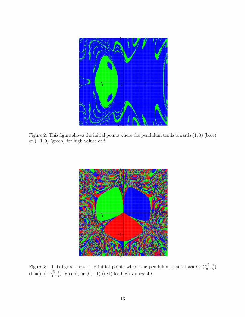
Figure 2: This figure shows the initial points where the pendulum tends towards (1, 0) (blue)or (−1, 0) (green) for high values of t.

Figure 3: This figure shows the initial points where the pendulum tends towards (√32, 12)

(blue), (−√32, 12) (green), or (0,−1) (red) for high values of t.

13

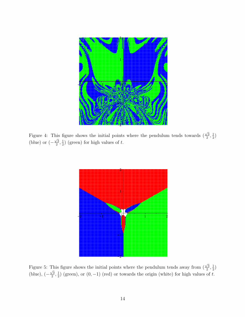
Figure 4: This figure shows the initial points where the pendulum tends towards (√32, 12)

(blue) or (−√32, 12) (green) for high values of t.

Figure 5: This figure shows the initial points where the pendulum tends away from (√32, 12)

(blue), (−√32, 12) (green), or (0,−1) (red) or towards the origin (white) for high values of t.

14

Figure 6: This figure shows the initial points where the pendulum tends towards (√32, 12)

(blue), (−√32, 12) (green), or (0,−1) (red) for high values of t.

Figure 7: This figure shows the initial points where the pendulum tends towards (√32, 12)

(blue), (−√32, 12) (green), or (0,−1) (red) for high values of t.

15

Figure 8: This figure shows the path taken by the pendulum when it starts at (1, 0).

Figure 9: This figure shows the path taken by the pendulum when it starts at (1, 0.05).

16