MAGNETIC NATURE OF INTRINSIC CARBON DEFECTS

Petri Lehtinen

Laboratory of PhysicsHelsinki University of Technology

Espoo, Finland

Dissertation for the degree of Doctor of Science in Technology to be presentedwith due permission of the Department of Engineering Physics and Mathemat-ics, Helsinki University of Technology for public examination and debate inAuditorium E at Helsinki University of Technology (Espoo, Finland) on the 4thof March, 2005, at 12 o’clock noon.

Dissertations of Laboratory of Physics, Helsinki University of TechnologyISSN 1455-1802

Dissertation 129 (2005):Petri Lehtinen: Magnetic Nature of Intrinsic Carbon DefectsISBN 951-22-7520-1 (print)ISBN 951-22-7521-X (electronic)

OTAMEDIA OYESPOO 2005

Abstract

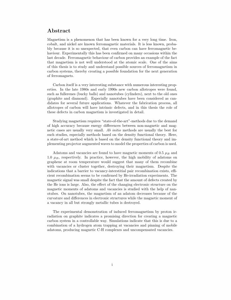
Magnetism is a phenomenon that has been known for a very long time. Iron,cobalt, and nickel are known ferromagnetic materials. It is less known, proba-bly because it is so unexpected, that even carbon can have ferromagnetic be-haviour. Experimentally this has been confirmed on many occasions within thelast decade. Ferromagnetic behaviour of carbon provides an example of the factthat magnetism is not well understood at the atomic scale. One of the aimsof this thesis is to study and understand possible sources of ferromagnetism incarbon systems, thereby creating a possible foundation for the next generationof ferromagnets.

Carbon itself is a very interesting substance with numerous interesting prop-erties. In the late 1980s and early 1990s new carbon allotropes were found,such as fullerenes (bucky balls) and nanotubes (cylinders), next to the old ones(graphite and diamond). Especially nanotubes have been considered as can-didates for several future applications. Whatever the fabrication process, allallotropes of carbon will have intrinsic defects, and in this thesis the role ofthese defects in carbon magnetism is investigated in detail.

Studying magnetism requires “state-of-the-art”-methods due to the demandof high accuracy because energy differences between non-magnetic and mag-netic cases are usually very small. Ab initio methods are usually the best forsuch studies, especially methods based on the density functional theory. Here,a state-of-art method which is based on the density functional theory and im-plementing projector augmented waves to model the properties of carbon is used.

Adatoms and vacancies are found to have magnetic moments of 0.5 µB and1.0 µB, respectively. In practice, however, the high mobility of adatoms ongraphene at room temperature would suggest that many of them recombinewith vacancies or cluster together, destroying their magnetism. Despite theindications that a barrier to vacancy-interstitial pair recombination exists, effi-cient recombination seems to be confirmed by He-irradiation experiments. Themagnetic signal was small despite the fact that the amount of defects created bythe He ions is large. Also, the effect of the changing electronic structure on themagnetic moments of adatoms and vacancies is studied with the help of nan-otubes. On nanotubes, the magnetism of an adatom decreases because of thecurvature and differences in electronic structures while the magnetic moment ofa vacancy in all but strongly metallic tubes is destroyed.

The experimental demonstration of induced ferromagnetism by proton ir-radiation on graphite indicates a promising direction for creating a magneticcarbon system in a controllable way. Simulations indicate that this is due to acombination of a hydrogen atom trapping at vacancies and pinning of mobileadatoms, producing magnetic C-H complexes and uncompensated vacancies.

i

Preface

This thesis has been prepared in the Laboratory of Physics in the CondensedComputational Matter and Complex Materials Group (Helsinki University ofTechonology, Finland) during the years 2001-2004.

I wish to thank Academy Prof. Risto Nieminen for the opportunity of work-ing in his group, advice, and ideas during this work. I also want to expressmy gratitude to my closest collaborators Dr. Adam Foster and Dr. YuchenMa for guidance. I would like to thank Prof. Kai Nordlund and Dr. ArkadyKrasheninnikov for the collaboration. Thanks also to the colleagues and thepersonnel in the laboratory. I acknowledge the computing resources providedby Center for Scientific Computing.

Finally, I would like to thank my parents and brother for support.

Espoo, October 2004

Petri Lehtinen

ii

Contents

1 Introduction 11.1 Carbon Atom and Hybridization . . . . . . . . . . . . . . . . . . 1

1.1.1 sp-Hybridization and Acetylene . . . . . . . . . . . . . . . 11.1.2 sp2-Hybridization and Graphite . . . . . . . . . . . . . . . 21.1.3 sp3-Hybridization and Diamond . . . . . . . . . . . . . . 41.1.4 Nanotubes . . . . . . . . . . . . . . . . . . . . . . . . . . 5

1.2 Intrinsic Magnetism in Carbon Systems . . . . . . . . . . . . . . 7

2 Introduction to Computational Methods 92.1 Density Functional Theory . . . . . . . . . . . . . . . . . . . . . 10

2.1.1 Basic Formalism . . . . . . . . . . . . . . . . . . . . . . . 102.1.2 Kohn–Sham Scheme . . . . . . . . . . . . . . . . . . . . . 122.1.3 Extension to Spin-Polarized Systems . . . . . . . . . . . . 132.1.4 Kohn–Sham Scheme in Spin-Polarized Systems . . . . . . 13

2.2 Approximations in DFT . . . . . . . . . . . . . . . . . . . . . . . 142.2.1 Approximation for Exchange-Correlation Functional . . . 142.2.2 Band Gap Problem . . . . . . . . . . . . . . . . . . . . . . 162.2.3 Plane Wave Basis Set and Supercell Approximation . . . 192.2.4 Pseudopotential Approximation . . . . . . . . . . . . . . . 202.2.5 Projector Augmented-Wave Method . . . . . . . . . . . . 20

2.3 VASP . . . . . . . . . . . . . . . . . . . . . . . . . . . . . . . . . 22

3 Magnetic Properties of Frenkel Pairsin Graphene 243.1 Introduction . . . . . . . . . . . . . . . . . . . . . . . . . . . . . . 243.2 Properties of Adatom on Graphene . . . . . . . . . . . . . . . . . 25

3.2.1 Equilibrium Position . . . . . . . . . . . . . . . . . . . . . 253.2.2 Migration of Adatom . . . . . . . . . . . . . . . . . . . . . 25

3.3 Clustering of Adatoms . . . . . . . . . . . . . . . . . . . . . . . . 263.4 Properties of Adatom on Nanotubes . . . . . . . . . . . . . . . . 28

3.4.1 Ground State Properties . . . . . . . . . . . . . . . . . . . 283.4.2 Migration of Adatom on Nanotubes . . . . . . . . . . . . 29

3.5 Vacancy in Graphene . . . . . . . . . . . . . . . . . . . . . . . . . 313.5.1 Migration of Vacancy in Graphene . . . . . . . . . . . . . 32

3.6 Vacancy in Nanotubes . . . . . . . . . . . . . . . . . . . . . . . . 33

4 Magnetism Stimulated by Non-Magnetic Impurities 36

5 Conclusions and Outlook 42

iii

A Spatial Correlations in Fluids 44

iv

List of Publications

This thesis consists of an overview and following publications:

I P. O. Lehtinen, A. S. Foster, A. Ayuela, A. V. Krasheninnikov, K. Nord-lund, and R. M. Nieminen, Magnetic Properties and diffusion of adatoms on agraphene sheet, Physical Review Letters 91, 017202 (2003).

II A. V. Krashennikov, K. Nordlund, P. O. Lehtinen, A. S. Foster, A. Ayuela,and R. M. Nieminen, Adsorption and migration of carbon adatoms on carbonnanotubes, Physical Review B 69, 073402 (2004).

III P. O. Lehtinen, A. S. Foster, A. Ayuela, T. T. Vehvilainen, and R. M.Nieminen, Structure and magnetic properties of adatoms on carbon nanotubes,Physical Review B 69, 155422 (2004).

IV Y. Ma, P. O. Lehtinen, A. S. Foster, and R. M. Nieminen, Magnetic proper-ties of vacancies in graphene and single-walled carbon nanotubes, New Journalof Physics 6, 68 (2004).

V P. O. Lehtinen, A. S. Foster, Y. Ma, A. V. Krasheninnikov, and R. M. Niem-inen, Irradiation-induced magnetism in graphite: a density-functional study,Physical Review Letters 93, 187202 (2004).

The author has had an active role in all the phases of the research reportedin this thesis. He has been involved in the planning of the calculations, ana-lyzing the results and representing the interpretation. The author has writtenthe main drafts for Publications I, III and V. The results calculated by theauthor provided a reference for the results presented in Publication II. In Pub-lication IV the author took part in calculating results of the graphene part andin interpreting the overall results.

v

Chapter 1

Introduction

1.1 Carbon Atom and Hybridization

Carbon is a group IV element in the Periodic Table of the Elements with thechemical symbol C, its atomic number is six, and atomic weight 12.01 g/mol[1]. Carbon has four valence electrons in the 2s2p2-configuration and two coreelectrons in the 1s-orbital. In order to form bonds, the atoms’ orbitals have toundergo a hybridization process, and carbon can have (acetylene) sp-, (graphite)sp2-, and (diamond) sp3-hybridizations while the other group four elements(Si,Ge, etc.) appear primarily in the sp3-hybridization.

1.1.1 sp-Hybridization and Acetylene

In gas welding, acetylene (C2H2) is one of the two main gases, oxygen (O2) isthe other. In acetylene, carbons undergo a simple sp-hybridization (see Figure1.1). A quantum mechanical description of the hybridization can be presented

Figure 1.1: sp-hybridization [2].

as a linear combination of atomic orbitals. In the sp-hybridization, sp-orbitalscan be presented as

|spa〉 = C1|2s〉 + C2|2px〉|spb〉 = C3|2s〉 + C4|2px〉,

(1.1)

where Ci:s are coefficients. These coefficents are determined from the require-ments, which the orbitals must satisfy, namely 〈spa|spb〉 = δab (orthogonalityand norm). Additionally, |2s〉 and |2px〉 can be presented in terms of |spi〉. Thenorm of |2s〉 and |2px〉 equals one. These conditions provide four equations for

1

the Ci:s, which are then ⎧⎪⎪⎪⎨⎪⎪⎪⎩C1C3 + C2C4 = 0C2

1 + C22 = 1

C22 + C2

3 = 1C2

3 + C24 = 1.

(1.2)

Solving Equation (1.2) the result is

|spa〉 =1√2

(|2s〉 + |2px〉)

|spb〉 =1√2

(|2s〉 − |2px〉) .(1.3)

The hybridized orbitals’ property is that they are larger in amplitude in onedirection and smaller in the other. The |spa〉 orbital is stronger or elongatedin the positive x-direction while weaker or shrunk in the negative x-direction.If the nearest neighbor is then in the positive x direction, the overlap betweensuitably hybridized orbitals increases, resulting in lower total energies (this isalso called as the σ bond). The remaining two electrons are perpendicular tothe hybrid orbital, and they interact with p-orbitals of the nearest neighbor,and form a weaker bond known as the π-bond [3] (see Figure 1.2).

Figure 1.2: Schematic presentation of acetylene [4].

1.1.2 sp2-Hybridization and Graphite

Pencils are probably the most commonly used application of graphite, which iscomposed of layered networks of hexagons. Layers are easily removed due toweak van der Waals bonds while the network is harder to break. Each carbonatom has three nearest neighbors in the plane, and the hybridization process,called sp2-hybridization, is thus different from the one in acetylene (see Figure1.3). In the sp2-hybridization, three out of four carbon’s valence electrons areinvolved in the mixing of orbitals, and the angle between the three orbitals is120. This means that the hybridized orbitals are in the directions (0,-1,0),(√

3/2,1/2,0), and (-√

3/2,1/2,0). The orbitals are then made as follows:⎧⎪⎪⎨⎪⎪⎩|sp2

a〉 = C1|2s〉 +√

1 − C21 |2py〉

|sp2b〉 = C2|2s〉 +

√1 − C2

2

[√3

2 |2px〉 + 12 |2py〉

]|sp2

c〉 = C3|2s〉 +√

1 − C23

[−

√3

2 |2px〉 + 12 |2py〉

].

(1.4)

From orthonormal requirements of |sp2a〉, |2s〉 and |2p〉, the constants (Ci) can

be solved with results: C1 = C2 = 1/√

3 and C3 = −1/√

3. A schematicpresentation of different bonds in graphene (one layer of graphite) is presentedin Figure 1.4

2

Figure 1.3: sp2-hybridization [2].

Figure 1.4: Schematic presentation of graphene [4].

3

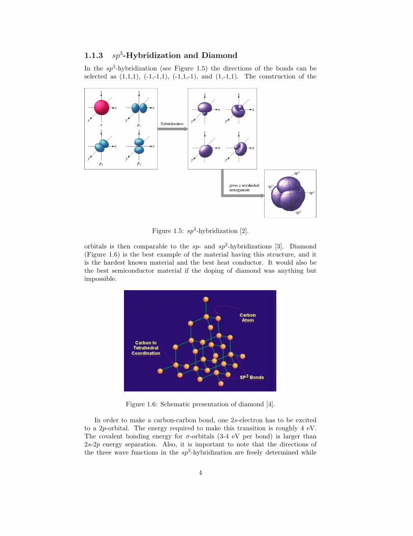
1.1.3 sp3-Hybridization and Diamond

In the sp3-hybridization (see Figure 1.5) the directions of the bonds can beselected as (1,1,1), (-1,-1,1), (-1,1,-1), and (1,-1,1). The construction of the

Figure 1.5: sp3-hybridization [2].

orbitals is then comparable to the sp- and sp2-hybridizations [3]. Diamond(Figure 1.6) is the best example of the material having this structure, and itis the hardest known material and the best heat conductor. It would also bethe best semiconductor material if the doping of diamond was anything butimpossible.

Figure 1.6: Schematic presentation of diamond [4].

In order to make a carbon-carbon bond, one 2s-electron has to be excitedto a 2p-orbital. The energy required to make this transition is roughly 4 eV.The covalent bonding energy for σ-orbitals (3-4 eV per bond) is larger than2s-2p energy separation. Also, it is important to note that the directions ofthe three wave functions in the sp3-hybridization are freely determined while

4

Figure 1.7: TEM images of multi-wall coaxial nanotubes with various inner andouter diameters, di and do, and numbers of cylindrical shells N: reported byIijima using TEM: (a) N=5 do=67 A,(b) N=2, do=55 A, and N=7, di = 23 A,do=65 A. [5]

the fourth direction is determined by the orthonormality conditions imposed onthe 2p-orbitals. This fact gives rise to possible sp2-hybridization of a planarpentagonal (or heptagonal) carbon ring, and sp2+η-hybridization (0 < η < 1),which is found in fullerenes. It is expected that the sp2+η hybridization has ahigher excitation energy than the symmetric sp2-hybridization because of theelectron-electron repulsion, which occurs in the hybridized orbital [3].

1.1.4 Nanotubes

Carbon nanotubes were discovered by Iijima in 1991 (see Figure 1.7 [5]). Theyare essentially single sheets of graphite (graphene) rolled into a cylinder. Ifthere are nanotubes inside each other, these are called multi-wall nanotubes.The diameter of a single-wall nanotube is less than few hundred angstromswhile the length scale is in the micrometer range.

The three most common methods to synthesize nanotubes are arc discharge,chemical vapour deposition (CVD), and laser ablation (vaporization). In thearc discharge method two graphite rods, which are a few millimeters apart,are connected to a power supply. Carbon atoms are vaporized into a plasmaand nanotubes are formed at the rod connected to the negative electrode where30 to 90% of the carbon consumed is converted to nanotubes. The single-walled nanotubes produced have diameters between 0.6-1.4 nm while multi-wallnanotubes’ inner tube have diameter in range 1-3 nm and outer tube’s diameteris approximately 10 nm. The tubes are short and they appear in random sizesand directions, which means that lot of purification is needed. With the arcdischarge method single- and multi-wall nanotubes are easily produced, andthey have few structural defects. In the CVD method, a substrate is placed inan oven, which is heated up to 600 C and carbon bearing gas such as methane isslowly added. As the gas decomposes, carbon atoms are free and recombine intonanotubes. Typical yield is between 20-100%. Tubes are long with diametersof 0.6-4 nm in single-wall and 10-240 nm in multi-wall nanotubes. The CVD

5

Figure 1.8: Chirality vector. The nanotubes having chirality vector marked witha green ball are metals in the sense of zone-folding. The rest are semiconductors.[7]

method is the best candidate for industrial purposes since the process is theeasiest to scale up and simple. Single-wall nanotube’s diameter can be controlledand resulting tubes are relatively pure. Most of the produced nanotubes are,however, multi-walled and riddled with defects. In the laser ablation method,graphite is heated with intense laser pulses. A pulsing lasergenerates carbongas, from which the nanotubes are formed with up to 70 % yields. Single-walltube bundles are long, 5-20 microns, and individual diameter varies between 1-2nanometers. The diameter control is good and there are few defects. Synthesisof multi-wall nanotubes with this method is not too attractive since it is tooexpensive [3, 6].

The electronic structure of a nanotube depends on how it is rolled, and isdesignated by a pair of letters (n,m), which is also called the chirality vector.The meaning of these letters can be explained with the help of Figure 1.8.The chirality vector starts at (0,0) and ends at (n,m). Then combining thestarting point and the end point we have a tube that we wanted. If the tubeis designated as (n,0), the tube is called a zigzag nanotube. If the tube is ofthe form (n,n), the tube is an armchair nanotube. The rest in between arecalled achiral nanotubes. The determination of whether a tube is a metallic orsemiconducting, is as follows: if n − m is divisible by 3, the tube is metallic;otherwise it is semiconducting. This can be understood in terms of zone foldingand analogy to graphite - the degenerate π and π∗ bands (the asterisk standsfor antibonding; usually not occupied, above the Fermi-level) in the graphiteBrillouin zone are folded into the Γ point in a nanotube [8, 9, 10, 11]. However,this type of description does not take into account the effect of curvature. Dueto the curvature of the nanotube, the π∗ and σ∗ orbitals hybridize, and thus asmall gap opens in zigzag nanotubes. This effect is the strongest in nanotubes,which have radius less than that of C60 [3].

6

1.2 Intrinsic Magnetism in Carbon Systems

Observations of magnetism in various carbon systems [12, 13, 14] have stimu-lated much experimental and theoretical research work (Ref. [15] and referencestherein) on the magnetic properties of all-carbon systems. The driving forcebehind these studies was not only to create technologically important, light,non-metallic magnets with a Curie point well above room temperature, but alsoto understand a fundamental problem: the origin of magnetism in a system,which traditionally has been thought to show diamagnetic behavior only.

The question, which immediately springs to ones mind is whether magnetismis an intrinsic property of carbon systems or is due to the presence of mag-netic impurities (e.g., Fe). The debate was initiated from the appearance ofthe two classic papers: in 2000 Kopelevich and coworkers published a paper[12] with an editor’s note of the controversial nature of the result. In thatwork, the authors identified ferromagnetic and superconducting-like magneti-zation hysteresis loops in highly oriented pyrolytic graphite samples below andabove room temperature. The conclusion was that magnetic impurities wereextremely unlikely. In 2001 Makarova and coworkers [13] reported a discoveryof strong magnetic signals in rhombohedral C60. Their intention was to searchfor superconductivity in polymerized C60; however, it appeared that their high-pressure, high-temperature polymerization process resulted in a magneticallyordered state. The material exhibited features typical of ferromagnets: sat-uration magnetization, large hysteresis and attachment to a magnet at roomtemperature. A careful analysis carried out in the original [13] and follow-upworks [14, 16, 17] showed that one can exclude magnetic impurities as the originof ferromagnetism.

If magnetism is indeed the intrinsic property of all-carbon systems, then themost important questions to be answered are as follows:

1. What is the atomic structure of the magnetic phase and what is the localbonding geometry, which gives rise to the net magnetic moment?

The presence of local magnetic moments can explain only the paramag-netic behavior but not ferromagnetism. Thus, the second question is:

2. How is the macroscopic ferromagnetic state formed and what is the mech-anism of the long-range order formation?

Because ferromagnetic signals have been detected in various carbon sys-tems such as graphite [12, 16], polymerized fullerenes [13], and carbonfoam [14], it is highly important to understand:

3. Is the mechanism of magnetic state formation common for all the carbonsystems or is it different for different allotropes?

Finally, if magnetism is not the intrinsic property of all-carbon systemsand it does not originate from magnetic impurities, then another questionarises:

4. Can magnetism result from impurity atoms, which are non-magnetic bythemselves, but due to unusual chemical environment, e.g., due to bondingto defects in graphitic network, give rise to local magnetic moments?

7

As for the first problem, a number of factors are nowadays thought to possi-bly give rise to the appearance of localized spins and the development of the mag-netic state in all-carbon systems: defects in the atomic network such as under-coordinated atoms [18, 19, 20, 21, 22, 23], itinerant ferromagnetism [24, 25] andnegatively-curved sp2-bonded nano-regions in the carbon structures [14, 26].Among these factors the defect-mediated mechanism appears to be the mostgeneral one because negatively-curved regions can hardly be found in graphite,and as for the second scenario, although itinerant mechanisms resulting fromstrong electron-elecron interactions and the effective dimensionality of the elec-tron system can give rise to magnetism, direct experimental evidence supportingsuch a mechanism is still lacking.

The defect-mediated mechanism has been addressed in a considerable num-ber of works [18, 19, 20, 21, 22, 23]. Although the details can be different fordifferent carbon systems (polymeric fullerenes, graphite, nanotubes), the com-mon feature is the presence of under-coordinated atoms, e.g., vacancies [21, 27],atoms on the edges of graphitic nano-fragments with dangling bonds either pas-sivated with hydrogen atoms [22, 23, 28] or free [20, 23]. Structural defects, ingeneral, give rise to localized electronic states, a local magnetic moment, flatbands associated with defects and thus to an increase in the density of statesat the Fermi level, and eventually to the development of magnetic ordering.However, even if this conjecture is correct, it is not clear at all whether suchdefects are actually present, or if their concentration is high enough to providethe magnetic moment observed in the experiments.

At the same time, it is well known that irradiation of carbon systems withenergetic electrons and ions should give rise to defects, and their number can becontrolled by choosing the right irradiation dose, particle energy and irradiationtemperature. Thus, if irradiation of the originally non-magnetic carbon samplesgave rise to magnetism, this could be strong evidence for the defect scenario.

Graphite samples were recently irradiated with 1.5 MeV He and 2.25 MeV Hions [29]. It was found that proton bombardment produced a strong magneticsignal, while bombardment with helium ions produced a signal, which was onlyslightly larger than background.

To explain the irradiation-induced magnetism and shed light on the role ofdefects in all-carbon magnetism, the atomic structure and magnetic moment ofvarious defects is studied in this thesis at the atomistic level within the frame-work of Density Functional Theory (DFT). The importance of the behavior ofvarious point defects–vacancies, interstitials and more complicated aggregations,both intrinsic, and those, which can appear in carbon nanotubes and graphiteunder irradiation to properties of material is addressed. Not only magnetic,but also structural and other characteristics of the defects are described, suchas formation energies and diffusivity. It is shown that under certain conditionsthe defects can indeed give rise to magnetism. Defects, which can appear underproton irradiation are considered, and the fact that even a small amount ofhydrogen in carbon samples might be very important for the formation of themagnetic state is demonstrated.

8

Chapter 2

Introduction toComputational Methods

Modern atomistic modeling techniques can be divided into three parts [30]:

1. Molecular mechanics uses classical physics and is computationally cheapsince it is very fast even with limited computer resources. It can be usedto calculate large systems like enzymes, which may have thousands ofmolecules. This means that the primary users are in the area of biologi-cal physics. Molecular mechanics does not calculate electronic properties,which prohibits bond breaking. Instead, molecular mechanics requires abinitio or experimental data on which the force fields it uses are parame-terized.

2. Semi-empirical methods use quantum physics but are computationally lessdemanding than ab initio methods. The idea is to use a relatively simplemolecular-orbital theory to define the potential surface of interest in sucha way that it can be adjusted to match ab initio calculations or exper-iment. The adjustments are usually made either by varying parametersthat arise naturally in the semiempirical calculations or by adding locallydefined correction functions to the semiempirical surface in order to “fixup” special regions of the potential surface such as barriers or minima [31].This means the usage is in the medium sized systems with hundreds oreven a few thousands of atoms. They too, however, rely on ab initio orexperimental data.

3. Ab initio or “the first principles” methods are also based on quantumphysics. They are mathematically very rigorous in the sense that they donot have empirical parameters. Ab initio methods are very useful for abroad range of systems. Computationally they are extremely expensiveand this limits the size of the system to little over 100 atoms. The usageis in systems requiring high accuracy, and flexible atomic environments.

In the following studies Ab initio techniques are used by applying densityfunctional theory (DFT) to find the ground state of the system. A brief outlineof DFT is given by following closely Ref. [32].

9

2.1 Density Functional Theory

2.1.1 Basic Formalism

The Hamiltonian of an interacting many-particle system is

H = T + V + W , (2.1)

which can be written in the second-quantized formalism as

H =∑α

∫d3r

[ψ†

α(r)(−

2

2m2 + v(r)

)ψα(r)

]

+12

∑αβ

∫d3r

∫d3r′ψ†

α(r)ψ†β(r′)w(r, r′)ψβ(r′)ψα(r).

(2.2)

In the nanometer scale, the dominant inter-particle interaction is the Coulombinteraction. The problem to solve, in general, is an eigenvalue problem, namely

H |Φ〉 = (T + V + W )|Φ〉 = E|Φ〉. (2.3)

Assuming that the situation to deal with is such that the ground state is non-degenerate, a member |Ψ〉 belonging to family of |Φ〉 provides the lowest eigen-value (|Φ〉 is a solution of the Schrodinger equation, |Ψ〉 is the one, which givesthe lowest energy), i.e. the ground state energy:

H |Ψ〉 = Egs|Ψ〉. (2.4)

The ground state density can then be calculated from

n(r) = 〈Ψ|∑α

ψ†α(r)ψα|Ψ〉

= N∑

α

∫d3x2, ...,

∫d3xN |Ψ(rα, x2, ..., xN )|2,

(2.5)

which is then a functional of v(r); the idea was first presented in [33]. Theparticle number (N) and the ground state density (n(r)) are related throughthe configurational distribution function, which also gives one of the sum rulesin the local density approximation (see appendix A).

The one to one correspondence between the density and the potential v(r) isproved by first recognizing that two potentials, V and V ′, always lead to differentground states |Ψ〉 and |Ψ′〉 if the potentials differ more than a constant, i.e.

V = V ′ + const. (2.6)

Eigenvalue equations for both potentials are

(T + V + W )|Ψ〉 = Egs|Ψ〉 (2.7)

and(T + V ′ + W )|Ψ′〉 = E′

gs|Ψ′〉. (2.8)

If |Ψ〉 and |Ψ′〉 are the same, the result is

(V − V ′)|Ψ〉 = (Egs − E′gs)|Ψ〉, (2.9)

10

which violates Equation (2.6). In the second phase of the proof, one must showthat |Ψ〉 = |Ψ′〉 implies n(r) = n′(r). Due to the Ritz principle

Egs = 〈Ψ|H |Ψ〉 < 〈Ψ′|H |Ψ′〉 (2.10)

and

〈Ψ′|H |Ψ′〉 = 〈Ψ′|H ′ + V − V ′|Ψ′〉 = E′gs +

∫d3r n′(r)[v(r) − v′(r)]. (2.11)

The combination of (2.10) and (2.11) gives

Egs < E′gs +

∫d3r n′(r)[v(r) − v′(r)]. (2.12)

By writing the corresponding argument for E′gs, using the assumption n(r) =

n′(r), and adding with Equation (2.12) the result will be

Egs + E′gs < Egs + E′

gs. (2.13)

The statements of the Hohenberg–Kohn theorem can then be formulated asfollowing:

• The ground state expectation value is a unique functional of the exactground state density

〈Ψ[n]|O|Ψ[n]〉 = O[n].

• Energy functional has variational character:

Ev0 [n] = 〈Ψ[n]|T + W + V0|Ψ[n]〉,

where V0 is the external potential of a specific system with ground statedensity n0(r) and ground state energy E0. By virtue of the Rayleigh–Ritzprinciple Ev0 [n] has the property

E0 < Ev0 [n], ifn = n0 (2.14)

andE0 = Ev0 [n0]. (2.15)

Hence, the ground state can be determined from

E0 = minnEv0 [n]. (2.16)

• T and W do not depend on the V0 of the particular system, and hence,the total energy functional may be written as

Ev0 [n] = FHK [n] +∫d3r n(r)v0(r), (2.17)

whereFHK = 〈Ψ[n]|T + W |Ψ[n]〉.

Thus, FHK is universal.

11

2.1.2 Kohn–Sham Scheme

The idea of creating something, which became to known as the Kohn–Shamequations [34] rose, according to Walter Kohn [35], from descriptional differencesbetween the so-called Thomas-Fermi theory and the Hartree equations. Thedifference between those two theories was in the treatment of the kinetic energyterm.

A system of N non-interacting particles described by the Hamiltonian

H = T + VS (2.18)

has a unique total energy functional

ES [n] = TS [n] +∫d3r vS(r)n(r), (2.19)

which has, according to the variational principle, the ground state density nS(r)corresponding to Equation (2.18). A central piece in establishing the Kohn–Sham scheme is that for any interacting system, there exists a local single-particle potential vS(r) such that the exact ground state density of the inter-acting system equals the ground state density of the non-interacting system,namely

n(r) = nS(r).

The ground state density has then a unique representation (non-degeneracyassumed)

n(r) =N∑

i=1

|ψ(r)|2 (2.20)

in terms of the lowest single-particle orbitals obtained from the Schrodingerequation (

− 2

2m2 + vS(r)

)ψi(r) = εiψi(r), ε1 ≤ ε2 ≤ .... (2.21)

Rewriting the total energy functional (2.17) into form

Ev0 [n] = TS [n] +∫d3r n(r)v0(r) +

12

∫d3r

∫d3r′ n(r)w(r, r′)n(r′) + EXC [n]

(2.22)the exchange-correlation functional EXC [n] is formally defined as

EXC [n] = FHK [n] − 12

∫d3r

∫d3r′ n(r)w(r, r′)n(r′) − TS [n]. (2.23)

The kinetic energy term in (2.22) has now changed from T [n] to TS[n], whichcan be written in terms of single-particle orbitals

TS[n] =N∑

i=1

∫d3r ψ∗(r)

(−

2

2m2

)ψ(r). (2.24)

Using the facts that Hohenberg–Kohn variational principle ((2.14),(2.15)) en-sures that Ev0 [n] is stationary for small variations δn around the minimum

12

density n0(r), single-particle orbitals satisfy Equation (2.21), and that the or-bitals are normalized, an expression for single particle potential, which generatesn0(r) via Equation (2.20) can be derived. The result is

vS,0(r) = v0(r) +∫d3r′ n0(r′)w(r, r′) + vXC([n0]; r), (2.25)

where

vXC([n0]; r) =δEXC [n]δn(r)

∣∣∣∣n0

. (2.26)

2.1.3 Extension to Spin-Polarized Systems

In spin-polarized systems, V in (2.1) needs to be extended in general to

V =∫d3r [v(r)n(r) − B(r) · m(r)], (2.27)

where the density operator is

n(r) =∑α

ψ†α(r)ψα = n+(r) + n−(r) (2.28)

and the magnetic moment density is

m(r) = −µ0

∑αβ

ψ†ασαβ(r)ψβ , (2.29)

where σαβ is a Pauli spin matrix and in particular

m(r) = −µ0(n+(r) + n−(r)). (2.30)

The difference of this formalism compared to the standard one is that insteadof trying to find only the ground state density, the objective is to find a fourvector (n(r),m(r)) for the non-degenerate ground state. The one-to-one cor-respondence between the ground state and the ground-state densities can beestablished through a similar argument as in (2.10) and (2.11). This fact isenough to establish the variational principle. According to Ref. [32] there isnot any proof that there is one-to-one correspondence between unique externalpotential (v(r),B(r)) and a given ground state. However, in the limit B → 0this formalism leads to a suitable description of systems having a spin-polarizedground state even without an external magnetic field (and in this case one-to-one correspondence between external potential and the state holds, although,the z-component of magnetic moment can have either positive or negative sign).

2.1.4 Kohn–Sham Scheme in Spin-Polarized Systems

For later purpose, and for notational simplicity, the external magnetic field B(r),and magnetization m(r) have only z-components

B(r) = (0, 0, B(r))

m(r) = (0, 0,m(r)).

13

The Kohn–Sham equation for the spin-polarized scheme consists of the followingequations:(−

2

2m2 + v(r) − αµ0B(r) +

∫d3r′ n0(r′)w(r, r′) + vXC([n+, n−]; r)

)ψ

(α)i (r)

= εiψ(α)i (r), ε(α)

i ≤ ε(α)2 ≤ ....

(2.31)

where α = + or− and

nα(r) =∞∑

i=1

γ(α)i |ψ(α)

i (r)|2, (2.32)

with γ(α)i satisfying the following relations

γ(α)i = 1 , ε(α)

i < µ(α)

γ(α)i ≤ 1 , ε(α)

i = µ(α)

γ(α)i = 0 , ε(α)

i > µ(α)

∞∑i=1

γ(α)i = Nα , N+ +N− = N.

(2.33)

The exchange-correlation potentials are defined as

v(α)XC([n+, n−]; r) =

δEXC [n]δnα(r)

∣∣∣∣n0

, (2.34)

and the functional EXC [n+, n−] is defined as

EXC [n] = FL[n+, n−] − 12

∫d3r

∫d3r′ n(r)w(r, r′)n(r′) − TL[n+, n−]. (2.35)

FL[n+, n−] is an extension of FHK to include degenerate states and constrainedsearch, whereas TL can be written as

TL[n] =N∑

i=1

γ(α)i

∫d3r ψ∗

α(r)(−

2

2m2

)ψα(r). (2.36)

2.2 Approximations in DFT

2.2.1 Approximation for Exchange-Correlation Functional

Local (Spin) Density Approximation

One problem of the density functional theory is that the exchange-correlationenergy functional defined in (2.35) is not known. EXC is composed of the kineticenergy part and the interaction part. With the help of Equation (2.2) a fewwords can be said of the interaction part, which is the one that usually is dividedinto the exchange and correlation parts. With the help of Wick’s theorem, anexpansion of the expectation value into direct and exchange parts can be made.

14

In the homogeneous electron gas model (rotational and translational symmetry,ion cores considered as neutralizing background) the direct part cancels alongwith the contributions from the background and electron-background interactionto the total energy. So the problem is to study the exchange term perturbatively.The exchange term (in terms of Feynman diagrams, see Figure 2.1(a)) in thefirst order produces the well-known result for the exchange energy

Figure 2.1: (a) Hartree-Fock energy diagrams. Because of the translational sym-metry and the uniform charge background, only the first diagram is nonzero fora uniform electron gas. (b) The first diagram gives the second order pertur-bation on the kinetic energy. Each cross represents a density vertex with themomentum of the external field. [36]

Ex

N= −e2 3

4π(3π2n

)1/3 12

[(1 + ξ)4/3 + (1 − ξ)4/3

], (2.37)

where ξ = (N+ − N−)/N [37]. The second order diagrams contributing tothe exchange-correlation energy can be found in Figure 2.2. Figure 2.2(a) iswell behaved (see for example Ref. [37]) while 2.2(b) is divergent. In higherorder terms, contribution from diagrams resembling Figure 2.2(b) are the fastestdiverging. In the high density limit, a summation of the fastest diverging termscan be done exactly [38, 39]. In the low-density limit, energy per particle canbe computed exactly [40, 41, 42], from which the correlation contribution canbe calculated. The remaining task is to find an expression for arbitrary densityand spin-polarization. One of the most noteworthy parameterizations can befound in Ref. [43] where the high-density limit of electron gas, scaling relationof spin-polarized ring approximation and Monte-Carlo results by Ceperley andAlder [44] are taken into account [32]. The method described above is knownas the local density approximation (LDA) or the local spin-polarized densityapproximation (LSDA). LDA has been highly successful because it fulfills theso-called sum rules of the exchange-correlation hole. Its deficiencies are thatit inadequately cancels the self-interaction contributions. The consequence isthat the local exchange-correlation potential does not exhibit correct asymptoticbehavior proportional to 1/r for localized systems (atoms, molecules etc.).

15

(a)(b)

Figure 2.2: Second order diagrams contributing to exchange-correlation energy.Fig. (a) is the second order exchange contribution and well behaving while Fig.(b) is the first order correlation diagram contributing to the correlation energy.

Generalized Gradient Approximation

In order to improve LDA/LSDA the simplest thing to do is to include gradientterms of the density into the functional. The functional built is known as thegradient expansion approximation (GEA). The difference between LDA andGEA is that instead of being free particles and holes in Figures 2.1 and 2.2,they are experiencing an external potential. This modifies the calculation ofthe correlation energy in the high density limit [36]. In later work, it wasrealized that GEA violates the sum rules of the exchange-correlation hole. Inorder to enforce the sum rules of the exchange hole, a real space cut-off wasintroduced [45]. A similar treatment had to be done also for the correlationenergy functional [46] since the exchange and correlation have to be treated in abalanced way. This leads to a scheme known as PW91 [47]. A useful formula invisualizing and thinking about the nonlocality, or in comparing one GGA withanother is

EGGAxc [n↑, n↓] ≈

∫d3r n

(− c

rs

)Fxc(rs, ξ, s), (2.38)

where c = (3/4π)(9π/4)1/3, and −c/rs = ex(rs, ξ = 0) is the exchange energyper electron of a spin-unpolarized uniform electron gas, and Fxc is an enhance-ment factor showing the effects of the correlation [48].

The problem with LDA/LSDA and GGA is that they are both designedfor non-homogeneous electron gases. Hence, the long-range interaction of non-overlapping systems is neglected. The reason for this is that the integrals in-volved in the evaluating the diagrams shown in sub-subsection 2.2.1 are doneeither in k-space (for Fourier transforms a box is needed) or in the real spacewith a regularization (potential of the form exp[−λr]/r). This means van derWaals interactions (long range dipole-dipole interaction) are neglected and thecalculation of distance between the layers of graphite can not be correctly done.Recently, a work has begun to overcome this problem (see for example Refs.[49] and [50]).

2.2.2 Band Gap Problem

The definition of the exact band gap ∆ is [32]

∆ = I −A (2.39)

16

where I is the ionization potential

I = E(N − 1) − E(N), (2.40)

where E(N) refers to the energy (functional) of N particle system, and A is theelectron affinity

A = E(N) − E(N + 1). (2.41)

The definition of the chemical potential µ is

δEv[n]δn(r)

= µ. (2.42)

If nN is the ground state density of N particle system then the ground stateenergy can be written as EN = Ev[nN ]. The exact chemical potential can thenbe written as

µ(N) =∂EN

∂N, (2.43)

and with the help of the fractional particle formalism [32]

µ(N) =

−I(Z) whenZ − 1 < N < Z;−A(Z) whenZ < N < Z + 1.

(2.44)

This means that the band gap can be written in the form

∆ = −µ(N − δ) − µ(N + δ)(2.42)=

δEv[n]δn(r)

∣∣∣∣N+δ

− δEv[n]δn(r)

∣∣∣∣N−δ

n=n0

(2.22)=

δTS [n]δn(r)

∣∣∣∣N+δ

− δTS [n]δn(r)

∣∣∣∣N−δ

n=n0

+

δExc[n]δn(r)

∣∣∣∣N+δ

− δExc[n]δn(r)

∣∣∣∣N−δ

n=n0

≡ ∆KS + ∆xc.

(2.45)

In order to recognize the terms in Equation (2.45) the fractional particle for-malism has to be used with the fact that the chemical potential can be writtenas in Equation (2.42). First the Kohn–Sham total energy functional for N + δparticles can be written as

Ω+0 (δ) =

N∑i=1

εi + δεN+1 − 12

∫d3r

∫d3r′ nδ(r)w(r, r′)nδ(r′)

+ EXC([nδ]) −∫d3r vXC([nδ

0]; r)nδ(r),

(2.46)

and a similar equation for the N − δ particles

Ω−0 (δ) =

N−1∑i=1

εi + (1 − δ)εN − 12

∫d3r

∫d3r′ n−δ(r)w(r, r′)n−δ(r′)

+ EXC([n−δ]) −∫d3r vXC([nδ

0]; r)n−δ(r).

(2.47)

17

Subtracting Ω0 from Equation (2.46), and from Ω0 Equation (2.47), the resultis

Ω+0 (δ) − Ω0 = δεN+1 + (EXC([nδ+

] − EXC [n]) (2.48)

andΩ0 − Ω−

0 (δ) = δεN + (EXC [n] − EXC [n−δ]) (2.49)

since the other terms explicitly depend on the density and a small density changearound the ground state density does not change them. Dividing then Equations(2.48) and (2.49) with δ, taking δ to zero and subtracting them from each otheran equation corresponding to Equation (2.45) is obtained. The final result willbe then

∆ = εN+1 − εN +∂EXC [nδ]

∂n

∣∣∣∣N+δ

− ∂EXC [nδ]∂n

∣∣∣∣N−δ

. (2.50)

If ∆xc (ie. a discontinuity of derivative of µ(N) at N = Z) is the reason forthe band gap problem, then changing the exchange-correlation functional doesnot improve the situation. The visible improvement is only a fluke since theunderlying reason behind the gap is still present.

A partial remedy to the question, which of the deltas is responsible for thegap was given by Godby, Schuter and Sham [51]. They calculated the exchange-correlation from equation [32]∫

d3y vXC(y)∫

dω

2πGs(r,y;ω)G(y, r;ω)

=∫d3y

∫d3y′

∫dω

2πGs(r,y;ω)Σxc(y,y′;ω)G(y′, r;ω),

(2.51)

where Σxc(y,y′, ω) is the irreducible self-energy, from which the local Hartreepotential has been substracted. Gs satisfies equation

(ω − hs)Gs = 1, (2.52)

where hs is the Kohn–Sham Hamiltonian. The full Green’s function can thenbe written by means of Dyson’s equation

G = Gs +GsΣG, (2.53)

where Σ is defined as

Σ = Σxc(y,y′;ω) − δ(r − r′)vXC(r). (2.54)

The connection to the particle density is

n(r) = −i∫dω

2πGs(r, r;ω) = i

∫dω

2πG(r, r;ω). (2.55)

Using the GW approximation for the self energy in (2.51), Godby, Schuter, andSham found an agreement between vXC in the local density approximation andvXC obtained in the fashion of Equations (2.51)-(2.55), as well as for the band-structures. The consequence is that the neglected discontinuity is the primarysource of error. For example, in the case of GaN the calculated band gaps (asin Ref. [52]) are between 1.76 eV and 3.0 eV in LDA calculations, and 1.45 eVin the GGA calculation compared to the experimental 3.41-3.65 eV.

18

2.2.3 Plane Wave Basis Set and Supercell Approximation

In electronic structure calculations, beside the exchange correlation energy, somethings have to be approximated or assumed. In the following, a brief outline ofthese technical issues is given.

In the preceding sections, it was shown how a many-particle problem canbe reduced to the effective single particle calculations. When looking at solids,the scale of the system is 1023 atoms. Even with non-interacting electrons,calculating their movement in that external potential would be a huge task.There are two challenges: a wave function must be calculated for each of thealmost infinite number of electrons in the system and since each electronic wavefunction extends over the entire solid the basis set required to expand eachwave function is almost infinite. With the help of the Bloch’s theorem the wavefunction can be divided into a cell-periodic part and wavelike part [53], namely

ψi(r) = exp[ik · r]fi(r), (2.56)

where the cell-periodic part of the wave function can be expanded using a basisset consisting of a discrete set of plane waves whose wave vectors are reciprocallattice vectors of the crystal

fi(r) =∑G

ci,G exp[iG · r]. (2.57)

The wave function can therefore written as

ψi(r) =∑G

ci,G exp[i(k + G) · r]. (2.58)

Electronic states are allowed only at a set of k points determined by theboundary conditions in the bulk. The infinite number of electrons in the solidare accounted by an infinite number of k points, and only a finite number ofelectronic states are occupied at each k point. Each electron in an occupiedstate contribute to the total energy and thus the number of needed k points isinfinite. Luckily, if the k points are close to each other the wave functions willbe almost identical. This means that the wave function at one k point presentsthe wave functions in the region of space. In order to calculate the electronicpotential and determine the total energy of the solid only finite amount of kpoints is required. Methods for approximating the electronic potential and totalenergy from filled electronic bands by calculating the electronic states at specialsets of k points in the Brillouin zone have been presented for example in Refs.[54]. In metals, a large amount of k points is needed while in insulators onlyfew to get good k point convergences.

When operating in k space, the terms with small kinetic energy 2/2m|k +

G|2 are usually more important (because of 1/k behavior of the Coulomb inter-action) than with a large kinetic energy. The plane-wave basis set can thereforebe truncated. In the process an error is made. When selecting a potential(pseudopotential, PAW, etc.) , it is necessary that with the selected cut-offenergy the total energies of the system are converged when compared to thelarger cut-off energies.

The Bloch’s theorem cannot be applied to a system with a defect. Calcula-tions with the plane-waves can only performed if a periodic supercell is used. A

19

supercell contains a defect with enough bulk around it to remove defect-defectinteractions between neighboring cells. This requires, of course, a set of testcalculations. The supercell is reproduced to fill the space to infinity [55].

2.2.4 Pseudopotential Approximation

The pseudopotential approximation makes use of the fact that the valence elec-trons are more important in determining the physical properties of a solid thanthe core electrons. In practise, this means that the Z/r behaviour of the coreelectrons is replaced by a weaker pseudopotential, which acts on a set of pseu-dowave functions rather than true valence wave functions (see Figure 2.3). Therapid oscillation of the valence wave functions in the region occupied by the coreelectrons due to the strong ionic potential maintain the orthogonality betweenthe core and valence wave functions required by the exclusion principle. Theconstruction of the pseudopotential is made so that its scattering properties orphase shifts for the pseudo wave functions are identical to the scattering prop-erties of the ion and the core electrons for the valence wave functions in such away that there are no radial nodes in the core region. In the core region, thetotal phase shift produced by the ion and the core electrons will be greater by πfor each node the valence functions had in the core region than the phase shiftproduced by the ion and the valence electrons. Outside the core region the twopotentials are identical, and the scattering from the two potentials is indistin-guishable. The phase shift produced by the ion core is different for each angularmomentum component of the valence wave function and so the scattering fromthe pseudopotential must be angular momentum dependent. The most generalform for a pseudopotential is then

VNL =∑lm

|lm〉Vl〈lm|, (2.59)

where |lm〉 are the spherical harmonics and Vl is the pseudopotential for angu-lar momentum l. This operator decomposes the electronic wave function intospherical harmonics and each of them is multiplied by pseudopotential Vl.

A pseudopotential that uses the same potential for all the angular momen-tum components of the wave function is called a local pseudopotential. In thiscase the pseudopotential is a function of the distance from the nucleus. It ispossible to produce arbitrary, predetermined phase shifts, but there are limitsto the amount that the phase shifts can be adjusted for the different angularmomentum states, while maintaining the smoothness and weakness of the pseu-dopotential. The shortcoming of this approach is the difficulty in expanding thewave functions using a reasonable number of plane-wave basis states [55].

2.2.5 Projector Augmented-Wave Method

A basic strategy of the augmented-methods is to divide space into regions,i.e. to make a partial-wave expansion near atom-centered sphere and envelopefunctions outside the spheres. The basic formalism in the Projector AugmentedWave-Method [56] is the following: A definition for a linear transformation is

τ = 1 +∑R

τR (2.60)

20

Figure 2.3: Schematic illustration of all-electron (solid lines) and pseudoelectron(dashed lines) potentials and wave functions. The radius at which all-electronand pseudoelectron values match is designated rc. [55]

where τR acts inside some augmentation region ΩR enclosing the atom. τRis defined for each augmentation region individually by specifying the targetfunctions |φi〉 for a set of initial functions |φi〉, which are orthogonal to the corestates and complete in ΩR, i.e. |φi〉 = 1+τR|φi〉. |φi〉 are called all-electron (AE)partial waves and |φi〉 pseudo (PS) partial wave functions. A natural choice forthe AE partial waves are solutions of the radial Schrodinger equation for theisolated atom, which are orthogonalized if necessary. A connection between PSand AE waves is that they are equal outside the augmentation region.

Considering an all-electron wave function (a full one-electron Kohn-Shamwave function), which can be presented as

|Ψ〉 = τ |Ψ〉 =∑

i

|φi〉ci, within ΩR, (2.61)

and a similar expression can be written for

|Ψ〉 =∑

i

|φi〉ci, within ΩR. (2.62)

The requirement that the transformation τ to be linear guarantees that the coef-ficients are linear functionals of the PS wave functionals. Hence, the coefficientsare scalar products

ci = 〈pi|Ψ〉, (2.63)

where the functions |pi〉 are called projector functions for each PS wave. Theprojector functions must fulfill the condition

∑i |pi〉〈φi| = 1 within ΩR. This

means that the one-center expansion∑

i |pi〉〈φi|Ψ〉 = |Ψ〉.In summary, Equations (2.61) and (2.63) define the linear transformation to

be used. The three quantities, which are determined from this transformationare:

21

• the AE partial waves |φi〉, obtained by radially integrating the Schrodingerequation of the atomic energy for a set of energies ε1i and orthogonalizationto the core states, i.e. the core state can be expressed as

|Ψc〉 = |Ψc〉 + |φc〉 − |φc〉 (2.64)

• PS partial wave |φi〉, which coincides with the corresponding AE partialwave outside some augmentation region for each AE partial wave

• one set of projector functions |pi〉 for each PS partial wave localized withinthe augmentation region, and obeys the relation 〈pi|φj〉 = δij .

The variational variable is |Ψ〉. The implementation of PAW-method into apseudopotential code can be done with relative ease (and it is done in Ref. [57]).One benefit of the PAW method is that it takes in a sense the core electronsinto account. The core region is well established. The approximation, which ismade in both pseudopotential and PAW calculations, is freezing the cores. Inthe search of energy minimum, modern computer algorithms can optimize theposition of ions using the Hellmann-Feynman forces [58, 59].

2.3 VASP

In this thesis the Vienna Ab Initio Simulation Package (VASP) is used asthe main work horse. VASP is a package for calculating ab-initio quantum-mechanical simulations using pseudo-potentials (PP) or the PAW-method withthe plane wave basis set. The execution time of parts of plane wave codes usuallyscales like N3 where N is the number of electrons in the system. In VASP theprefactors before the cubical term are negligible, leading to an efficient scalingwith respect to system size. This has been achieved by evaluating the non-local parts of the pseudo-potential in real space and by keeping the number oforthogonalisations at a minimum.

The implementation in VASP is based on the (finite temperature) LDA withthe free energy as a variational quantity and an exact evaluation of the instan-taneous electronic ground state at each MD step. VASP uses an efficient Pulay-Broyden charge density mixing. These techniques avoid all problems possiblyoccurring in the original Car–Parrinello method, which is based on the simulta-neous integration of electronic and ionic equations of motion. The interactionbetween ions and electrons by ultra-soft Vanderbildt pseudo-potentials (US-PP)or by the PAW-method. These pseudo-potentials and the PAW method allowfor a considerable reduction of the number of plane-waves per atom for transi-tion metals and first row elements. Generally, not more than 100 plane wavesper atom are required to describe the bulk properties of a solid. Forces and thefull stress tensor can be calculated easily, and used to relax atoms into theirinstantaneous ground state.

The combination of self-consistency cycle to calculate the electronic groundstate with efficient numerical methods has lead to an efficient scheme for evaluat-ing the self-consistent solution of the Kohn-Sham functional. The implementediterative matrix diagonalisation scheme is among the fastest available schemes.

The symmetry of an arbitrary configuration is automatically determined inVASP. The symmetry code is also used to set up the Monkhorst-Pack special

22

points allowing an efficient calculation of bulk materials and symmetric clus-ters. The integration of the band-structure energy over the Brillouin zone isperformed with smearing or tetrahedron methods [60, 61, 62].

23

Chapter 3

Magnetic Properties ofFrenkel Pairsin Graphene

3.1 Introduction

There are two main types of intrinsic defects: vacancies and interstitials, anddislocations. Vacancy means that one ion is missing and interstitial that thereis an extra ion in the crystal. These defects are usually the cause for the ob-served conductivity of ionic crystals, and they have a significant effect on theoptical properties (especially on the color). They are always present in thermalequilibrium, which makes them intrinsic in nature [53]. Dislocations are linedefects, and they do not have thermodynamic origin. Instead, dislocations arecaused by stresses affecting a sample during growth. Dislocations are essentialin explaining the observed strength (or lack of it) of real crystals and the ob-served growth rates [53]. Since recombination of proximate Frenkel partners isvery probable, in this section the properties of isolated adatoms and vacanciesin carbon systems are considered - specifically a graphene sheet and variousnanotubes.

Besides vacancies and interstitials, there are other types of simple defects,such as Stone-Wales defects (two heptagons and two pentagons), formed byrotating a carbon-carbon bond by 90 degrees [63]. The barrier for such defectformation is lower than that for Frenkel pairs, especially if an extra carbon atom,which works as a catalyst is nearby [64]. However, this defect is nonmagnetic,so it is not considered further.

The abundance of open space in nanotubes suggests that the interstitialatom can also be treated as an adatom adsorbed onto the nanotube surface [65,66]. This is particularly the case for isolated single-walled nanotubes (SWNT)and interstitials in the inner cores of the tubes. However, the nature of thevacancies and interstitials in graphite and multi-walled nanotubes (MWNT)is complicated by the presence of nearby layers. If graphite is considered asan example, it is clear that the properties of vacancies and interstitials maybe affected by the presence of the second layer. However, as discussed in theprevious section, any treatment of interlayer processes with DFT ignores thefact that the van der Waals interaction between layers is incorrectly represented.Hence, it is probably better, and still qualitatively correct, to consider only a

24

single graphene sheet as a good model of graphite.

3.2 Properties of Adatom on Graphene

3.2.1 Equilibrium Position

The first ab initio calculations concerning the properties of an adatom on asingle sheet of graphite (graphene) were performed by Mattila and coworkers[67] in the middle of 1990s. Using a 50-atom size sheet and LDA the authorsof that work concluded that the ground state of an adatom was in a bridge-likestructure.

The development of computing techniques and computers alongside the re-newed interest on the carbon materials made it tempting to recalculate theground state properties of the carbon atom on a sheet of graphite. Using GGAwith the full relaxation of the spin produced a whole set of results [68]: Theadatom is 1.87 A above the surface (2.0 A in Mattila’s studies), the distanceto the adatom’s nearest neighbors is 1.52 A and the distance between the near-est neighbors is 1.58 A. The adsorption energy was found to be 1.40 eV (3.30eV in Mattila’s studies and 1.2 eV in Heggie’s work [69], and 1.78 eV in Lee’swork [70]). A new property of the equilibrium position of adatom was thatthe ground state has a magnetic moment of 0.45 µB . The magnetism arisesfrom the interaction between the sp2- and unhybridized px-orbital, which trans-fers charge from the px-orbital to the dangling sp2-orbital (see Figure 3.1 [68]).The orbital-orbital interaction, which is the cause of the adatom’s magnetism,

Figure 3.1: (a) Spin density in e/A3 of plane normal to surface through centerof adatom when adatom is at equilibrium position. The adatom is at (0,0). (b)A Schematic diagram of bond orbitals at the equilibrium position in a planethrough the adatom and two surface carbons. Note that this schematic isa projection, and that the blue p-orbital is orthogonal to the adatom-surfacebonds.[68]

is caused by the breakdown of the symmetry of the sp2-hybridization. In thegraphene plane, the angle between each bond is 120. When three carbon atomsform a bridge structure, it is obvious that the angles differ from 120.

3.2.2 Migration of Adatom

The study of the migration path is crucial in determining the dynamics of thedefect. The migration energy path gives two important pieces of information:

25

The migration energy barrier tells how stable the defect is, i.e. how easilydefect’s properties can be measured, and the path provides information aboutwhat happens to the magnetism during the motion of the defect.

The calculated migration path of an adatom is almost a straight line (seeFigure 3.2). During the migration between the equilibrium positions, the mag-netic moment disappears because the adatom’s hybridization changes from sp2-to sp-like (only one bond attached to the surface) leaving one dangling bond,px-, and py-orbitals free. The p-orbitals then interact with themselves creat-ing π-orbitals, which interact then with the remaining sp-orbital. The result ismuch more delocalized density and the magnetism is destroyed. The migrationenergy barrier is 0.47 eV (Figure 3.3) (0.1 eV in Heggie’s work [69]). These factsmean that the adatom is highly mobile on the plane at room temperatures, andexperimental observation is difficult. The diffusion through the layers has anenergy barrier of 2.3 eV [71] making in-plane motion of an adatom favorable.

(a) (b)

Figure 3.2: Migration path of adatom on graphene from (a) top and (b) side.The starting point of the path is the equilibrium position and the end pointis another equilibrium position. They are both so-called bridge-like structures.The middle points of the path, where adatom has two bonds, is actually atransition point from magnetic to non-magnetic situation. The reason is thechange in the hybridisation of the adatom.

3.3 Clustering of Adatoms

Since it is known that adatoms are very mobile, an obvious question is whetherthey form clusters on the surface. The clusters have properties depending ontheir size, as will be shown. The smallest clusters, dimers and trimers, arestudied here.

The adsorption energy of a carbon atom above another carbon atom forming

26

0 2 4 6 8Position in the diffusion path

0

0.1

0.2

0.3

0.4

0.5

Ene

rgy

(eV

)

Spin polarizedSpin restricted

Figure 3.3: Migration energy barrier of adatom on graphene.[68]

the top of a bridge structure, as shown in Figure 3.4(a), is 8.7 eV. This systemis not magnetic since the the dangling sp2-bond of the bridge forms a bondwith the sp-orbital of the upper carbon ion. The px-orbital of the carbon ionat the bridge configuration interacts with the p-orbitals of the upper carbon ionbecoming π-orbital as in graphene. The reason why the sp-type dangling bonddoes not have a magnetic moment is as in the case of an adatom alone.

(a) (b)

Figure 3.4: Clustering of multiple adatoms. The equilibrium structure of twoadatoms (dimer) in Fig. 3.4(a) and three adatoms (trimer) in Fig. 3.4(b).

Making a similar calculation with a carbon trimer results in a linear C-C-Cequilibrium configuration parallel to the surface plane. Compared to the perfectgraphene sheet and three isolated carbon atoms this structure has 12.2 eV lowerenergy, demonstrating that adatoms will cluster on the surface. In contrast tothe dimer, the trimer is magnetic, but with a lower moment than the adatom(0.2 µB). Since C-C-C is composed of sp-bonds, the conclusion is that thedangling sp-bonds interact first with the p-orbitals preventing the formationof π-orbitals. In general, these results suggest that all clusters with an evennumber of atoms will be non-magnetic, and all odd will be magnetic - but themoment decays rapidly with the size of the cluster. However, any quantitativeconclusions would require an extensive study of cluster growth and include the

27

effects of interlayer interactions.

3.4 Properties of Adatom on Nanotubes

3.4.1 Ground State Properties

Because the structure and bonding in carbon nanotubes are very similar to thatof graphite, it is interesting to explore whether adatoms are also magnetic onnanotubes. The ground state of an adatom on nanotubes is in a bridge-like struc-ture as in graphite. There are slight differences in bridge-structures dependingon the position of the bridge and depending on a tube. Figures 3.5 and 3.6 showthe equilibrium positions of an adatom on zigzag and armchair nanotubes, re-spectively. The parallel position (the bridge is parallel to the translational axisof the tube) shown in Figures 3.5(a) and 3.6(a) is a metastable position, as canbe seen in the Table 3.1 [72], while perpendicular position (the Figures 3.5(b)and 3.6(b)) is the ground state position. The small zigzag nanotubes are semi-

(a) (b)

Figure 3.5: Equilibrium positions of adatom on (9,0) nanotube in (a) paralleland (b) perpendicular positions.

(a) (b)

Figure 3.6: Equilibrium positions of adatom on (5,5) nanotube in (a) paralleland (b) perpendicular positions.

conductors while the armchair nanotubes are always metals. This difference inthe electronic structure has an effect on the magnetic moment of an adatom.There are three factors to be considered when evaluating the magnetic moment

28

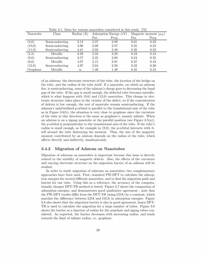
Table 3.1: Data for various nanotubes considered in this study. [72].Nanotube Class Radius (A) Adsorption Energy (eV) Magnetic moment (µB)

Par. Perp. Par. Perp(8,0) Semiconducting 3.13 2.37 2.89 0.01 0.23(10,0) Semiconducting 3.96 2.09 2.57 0.25 0.23(11,0) Semiconducting 4.41 2.03 2.49 0.20 0.22(5,5) Metallic 3.39 2.33 3.29 0.23 0.44(9,0) Semiconducting 3.57 2.35 2.80 0.24 0.35(6,6) Metallic 4.07 2.15 2.91 0.27 0.43(12,0) Semiconducting 4.97 2.04 2.50 0.32 0.36Graphene Metallic ∞ 1.40 1.40 0.45 0.45

of an adatom: the electronic structure of the tube, the location of the bridge onthe tube, and the radius of the tube itself. If a nanotube, on which an adatomlies, is semiconducting, some of the adatom’s charge goes to decreasing the bandgap of the tube. If the gap is small enough, the defected tube becomes metallic,which is what happens with (9,0) and (12,0) nanotubes. This change in elec-tronic structure takes place in the vicinity of the defect, so if the concentrationof defects is low enough, the rest of nanotube remain semiconducting. If theadatom’s unhybridized p-orbital is parallel to the translational axis of the tubeas in Figure 3.6(b), the situation is very close to graphene since the curvatureof the tube in this direction is the same as graphene’s, namely infinite. Whenan adatom is on a zigzag nanotube at the parallel position (see Figure 3.5(a)),the p-orbital is perpendicular to the translational axis of the tube. If the tube’sradius is small enough, as for example in (8,0), the p-orbital interacts with it-self around the tube destroying the moment. Thus, the size of the magneticmoment contributed by an adatom depends on the radius of the tube, whichaffects directly and indirectly, simultaneously.

3.4.2 Migration of Adatom on Nanotubes

Migration of adatoms on nanotubes is important because this issue is directlyrelated to the stability of magnetic defects. Also, the effects of the curvatureand varying electronic structure on the migration barrier of an adatom will bestudied.

In order to study migration of adatoms on nanotubes, two complementaryapproaches have been used. First, standard PW-DFT to calculate the adsorp-tion energies for several different nanotubes, and to find the migration path andbarrier for one tube. Using this as a reference, the accuracy of the computa-tionally cheaper DFT-TB method is tested. Figure 3.7 shows the comparison ofadsorption energies, and demonstrates good qualitative agreement - note thatthe PW-DFT results differ from the DFT-TB (using LDA) by a constant, whichmatches the difference between LDA and GGA in adsorption energies. Figure3.8 also shows that the migration barrier is also in good agreement, hence DFT-TB is used to calculate the migration for a large number of tubes. Figure 3.8shows the barrier as a function of radius for the armchair and zigzag tubes con-sidered. As expected, the barrier decreases with increasing radius, and tendstowards the limit of infinite radius, i.e. graphene.

29

Figure 3.7: Adsorption energies of carbon adatoms on zigzag (a) and armchair(b) single walled nanotubes as function of nanotube diameter. The arrowsvisualize the relationships between the corresponding TB and PW results. Thenumbers stand for the tube chirality indices. [73]

Figure 3.8: Energy barrier for adatom migration on the outer surface on nan-otubes as function of nanotube diameters. Here the graphene migration barrieris the same for the PW and TB calculations. [73]

30

3.5 Vacancy in Graphene

In order to remove a carbon ion from the carbon network, of which the grapheneis composed, 7.7 eV (calculated as in Ref. [74]) is needed in agreement withprevious DFT results of 7.6 eV [75] and 7.4 eV [76]. Atoms 1 and 2 (see Figure3.9) form a bond creating a pentagon. The distance between atoms 1 and 2is 2.02 A compared to the 1.42 A in graphene. Atom 3 is elevated from thesurface through the Jahn-Teller displacement of about 0.18 A (0.47 A and nomagnetism in Ref. [76]). The vacancy is magnetic with a magnetic moment of1.04 µB. The explanation is as follows: The removal of one carbon ion createsthree unsaturated sp2-orbitals in the neighboring carbon ions. The formationof the pentagon saturates two of them, which leaves one sp2-orbital free. Thisremaining dangling bond contributes the calculated magnetic moment as canbe seen in Figure 3.10.

Figure 3.9: (a) Atomic structure of vacancy in graphene plane. (b) The chargedensity of a vacancy in the graphene plane (e/A3). [77]

Figure 3.10: Spin density of vacancy in graphene plane (e/A3). [77]

31

3.5.1 Migration of Vacancy in Graphene

The calculated migration energy barrier of a vacancy is 1.41 eV (see Figure 3.12),which is in agreement with 1.7 eV in Ref. [78] and with previous studies [79, 80],but in disagreement with the experimental value of 3.1±0.2 [81]. Such a cleardisagreement between the experiments and theory suggests that experimentshave failed to measure the migration energy of a single vacancy, and instead themigration of divacancy is measured. Thus, it is clear that the interstitials movefaster than the vacancies in graphite. The inter-plane migration of a vacancy isa much more difficult with the experimental migration barrier of more than 5eV [81]. Thus, in-plane migration is favourable for both types of defects.

The migration path of a vacancy is shown in Figure 3.11 and the correspond-ing migration energy barrier in Figure 3.12. A bond rotation occurs betweenpoints 10-12 which costs 0.2 eV in agreement with calculations in Ref. [76].Points #3, #4, #6, #7 and #9 do not carry a net magnetic moment. The maindifference between points #4 and #5, and on the other hand points #8 and #9,is the bond length of the pentagon bond. In the non-magnetic cases it is 2.00A(#4) or 1.98 A(#9) while in the magnetic cases the length of the pentagonbond is 1.87 A(#5 and #8). The reason for this magnetic moment is in theformation process of a bond, which seems to start with spin-polarization of thesp2-orbital.

Figure 3.11: Migration path of vacancy in graphene.

0 1 2 3 4 5 6 7 8 9 10 11 12 13Point in Path

0

0.5

1

1.5

2

Ene

rgy

(eV

)

Figure 3.12: Migration energy barrier of vacancy in graphene.

32

Table 3.2: Properties of 5-ring armchair SWNTs with vacancies of differentconfigurations. [77]

Nanotube Configuration Efor (eV) Class Mag. (µB)(3, 3) Perp. 4.4 Semi. 0.0

Par. 5.2 Metal 1.0(4, 4) Perp. 5.3 Semi. 0.0

Par. 6.2 Metal 1.0(5, 5) Perp. 5.6 Metal 0.6

Par. 7.1 Semi. 0.0(6, 6) Perp. 5.9 Semi. 0.0

(Metal1) (0.41)Par. 7.3 Semi. 0.0

14-ring (6, 6) tube.

3.6 Vacancy in Nanotubes

The description of magnetic properties of a vacancy in nanotubes is much moredifficult task. The properties of a vacancy in a nanotube are due to an interplayof the following facts: first, nanotubes are cylinders, not flat planes. The ionsguarantee that a nanotube is a three dimensional object. The surroundingsof a vacancy may have more than one configuration, and all of them need tobe checked in order to find the ground state. Secondly, the size of the tubechanges when the chirality vector changes. This has an implication that aground state vacancy configuration may not be a general ground state for alltubes regardless of the chirality. Thirdly, in nanotubes the electronic structurevaries in perfect zigzag nanotubes between semiconducting and metallic, andthe perfect armchair nanotubes are always metallic. The electronic structurechanges easily when there are defects in the system. These facts mean a largeset of calculations, and the calculated results for different configurations (seeFigures 3.13(a) and 3.13(b) [77] ) are collected in Tables 3.2 and 3.3.

The configuration shown in Figure 3.13(c) has the following properties: Eachcarbon ion is sp2-hybridized. The carbon atom with a dangling bond has mag-netic moment of 1 µB and creates a metallic band. This metallic band is createdby the redistribution of the charge within the hexagonal carbon network of thenanotube. In this sense, the behavior is similar to the behavior of an adatomon a nanotube. However, the magnetic properties of a nanotube with a vacancydepend much more on the curvature of the tube than the properties of a nan-otube with an adatom because with a smaller tube the effect of removal of anatom is larger. If the Jahn-Teller effect seems to be of similar size in absolutescale, this means that the Jahn-Teller effect is much larger in smaller nanotubesin relative scale. The reason for larger Jahn-Teller effect in smaller tubes is thestress inherent in every nanotube, and in smaller nanotubes the stress is alwaysstronger than in larger nanotubes.

Figure 3.13(a) shows the ground state of the vacancies for (5,5) and (6,6)nanotubes. The (5,5) nanotube with a vacancy at the perpendicular configu-ration is magnetic because the Jahn-Teller distortion is large-enough to formthe bridge structure (although not sufficient to get 1 µB). The relaxations of

33

Table 3.3: Properties of 6-ring zigzag SWNTs with vacancies of different con-figurations. [77]

Nanotube Configuration Efor (eV) Class Mag. (µB)Perp. 4.6 Semi. 0.0

(5, 0)1 Par. 5.1 Semi. 0.02

3db 6.0 Semi. 0.02

(6, 0) Perp. 5.0 Metal 0.3Par. 5.8 Metal 0.9

(7, 0) Perp. 5.2 Semi. 0.0Par. 6.3 Metal 0.8

(8, 0) Perp. 5.3 Semi. 0.0Par. 6.5 Metal 0.8

(9, 0) Perp. 5.4 Semi. 0.0Par. 6.4 Metal 1.0Perp. 5.5 Semi. 0.0

(10, 0) Par. 6.7 Metal 0.93db 7.4 Metal 1.9

1 8-ring (5, 0) tube.2 Anti-ferromagnetic.

(a) (b) (c)

Figure 3.13: Ground state of vacancies in zigzag and armchair nanotubes. InFig. (a) are (5,5) (red) and (6,6) (opaque) armchair nanotubes and in Fig.(b) are (6,0) (opaque) and (9,0) (red) nanotubes. Although the nanotubes areshown inside each other they were calculated separately. In Fig. (c) calculatedproperties of tubes with a vacancy follow from the properties of this configura-tion.

34

the rest of the tube are small enough so that the overall electronic structureremains metallic. For the (6,6) nanotube, the Jahn-Teller effect is dependent onthe linear density of the vacancies along the tube. It is not large enough for amagnetic ground state if the density is less than 1 vacancy per 4 carbon rings.The smaller radii (3,3) and (4,4) armchair nanotubes demonstrate perfectly thebridge configuration, giving a magnetic moment of 1 µB in the parallel position.

The bridge configuration is also responsible for the magnetism and metallicelectronic structure of the parallel vacancy in larger zigzag-tubes such as (7,0),(8,0), (9,0) and (10,0) (see Fig. 3.13(b)). When the vacancy is in the perpen-dicular configuration, these tubes remain semiconductors, as the removal of theion increases the gap. The ideal (6,0) nanotube is metal, and no matter wherethe vacancy is located, it remains metallic and has a magnetic moment. (5,0)is a semiconductor due to an extensive damage on the networks caused by thevacancy on a small tube, preventing the formation of a metallic band.

The question as to what happens with an open ended nanotube was studiedin Ref. [23]. If the other end of a nanotube is capped with a fullerene, theauthors found that the edge atoms have a magnetic moment of 1.25 µB perdangling bond. If a nanotube has both edges open, the spins of the danglingbonds are antiferromagnetically ordered. If the dangling bonds at one edge aresaturated with hydrogen, the spins in the open edge contribute most to the totalmagnetic moment (1µB per atom). In the (8,0) nanotube the authors found asmall polarization of p-orbitals at carbons attached to the hydrogen atoms atthe edge. The magnetic state generated by vacancies, zigzag edges at nanotubeends, and defective fullerenes are very similar, and point very clearly to theflatband mechanism of magnetism already studied in Refs. [20, 82].

35

Chapter 4

Magnetism Stimulated byNon-Magnetic Impurities

In addition to creating intrinsic defects in carbon materials, ion irradiation mayalso lead to doping of the sample by the impinging ions. Specifically, the ir-radiation of graphite by protons has been shown experimentally to induce asignificant magnetic signal [29]. Since similar irradiation by helium ions pro-duces a much weaker signal, it cannot be simply explained by the generationof vacancies and adatoms. Hence, the properties of hydrogen and helium ingraphite via DFT-GGA simulations are considered, and whether they a playrole in the observed magnetism examined.

The adsorption energy of H on perfect graphene is 0.87 eV (0.71 eV inRef.[83], 0.76 eV in Ref. [84], 0.76 eV in Ref. [85] and 0.67 eV in Ref. [86]) andthe adsorption position is above another carbon ion. This configuration has nomagnetic moment unless the density of hydrogen on the surface is very high,i.e. approaching a few percent [85]. In any case, above a graphene sheet thehydrogen is quite mobile (barrier 1.30 eV for an isolated H on graphene, butreducing to 0.48 eV near other H atoms [84]) and does not form a dimer easilysince the barrier for recombination is 2.82 eV [84]. Hence, it is highly probablethat hydrogen migrates on the plane until it is pinned by another defect.

If the hydrogen encounters an empty vacancy, it saturates the dangling bond,and is pinned at a height of 1.25 A above the plane (Figure 4.1), with an adsorp-tion energy of 4.36 eV. This configuration is non-magnetic. This result contrastswith studies of the effect of a hydrogen on a vacancy-like defect in fullerenes [27],where a magnetic moment of 3.0 µB per C60-cage was observed. However, thelocal structure in the fullerenes is different, and the under-coordinated carbonscannot saturate bonds with each other due to the increased strain in the sys-tem. Hence, hydrogen saturates only one dangling bond and the local momentis provided by the other two sites. In the context of hydrogen migration througha layer, a similar configuration can be considered in graphene (see Figure 4.2),where hydrogen adsorbs directly into the vacancy, in-plane with the graphenesheet. The calculated migration path of a hydrogen through the graphite va-cancy is shown in Figure 4.3, and the migration barrier is 1.25 eV. In points #1,#2, #3, #4 and #5 a pentagon bond is formed, and the rest of the points are inthe process where hydrogen raises out of the plane. The saddle point (#0) is at

36

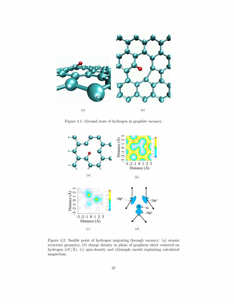
(a) (b)

Figure 4.1: Ground state of hydrogen in graphite vacancy.

(a)(b)

(c) (d)

Figure 4.2: Saddle point of hydrogen migrating through vacancy: (a) atomicstructure geometry, (b) charge density in plane of graphene sheet centered onhydrogen (eV/A), (c) spin-density and (d)simple model explaining calculatedmagnetism.

37

the graphite plane. This position of a hydrogen is magnetic. The reason is thatthe hydrogen forces the ions forming the base of pentagon to move away fromeach other (Fig. 4.2(a)). From the basis of Figure 4.2(b), which is the chargedensity of the vacancy site, it is certain that the pentagon bond is significantlyweakened. The resulting magnetic moment is 2.3 µB, and the spin-density (Fig.4.2(c)) shows that this is mainly due to two dangling bonds on the separatedcarbon. With the help of a simple model figure (Fig. 4.2(d)) the interpretationof the result is the following: The hydrogen’s 1s and one of the dangling bondsform a bond. The electron cloud around the hydrogen atom becomes thinnerand it attracts the electrons localized in the dangling bonds of the other nearestneighbor carbon atoms. Hence, the sp2-orbitals are directed toward the hydro-gen ion and do not bond with each other. These two dangling bonds contributea magnetic moment of 2 µB. Now the remaining magnetic moment comes fromthe 1s-sp2 bond. Since 1s is spherical, not all of its charge is committed to thebond; only half an electron is contributed to the bond making- but suppress-ing the magnetism of the sp2-bond a whole electron is required. Hence 1s-sp2

bond becomes magnetic and contributes a magnetic moment of 0.5 µB . Sincethe method used cannot describe the van der Waals interactions properly, it ispossible that in a multi-layered system this state becomes a deep metastableposition, but other configurations seem more likely.

0 1 2 3 4 5 6 7 8 9Point in Path

0

0.5

1

1.5

2

Ene

rgy

(eV

)

(a)

(b)

Figure 4.3: Migration (a) barrier and (b) path of hydrogen through graphitevacancy.

Two stable magnetic configurations involving hydrogen do exist in graphite.Firstly, if a hydrogen atom encounters a vacancy which has already been satu-rated by hydrogen, it will bond to the other side of the vacancy (see Fig. 4.4(a))with an adsorption energy of 3.2 eV, at a distance of 0.76 A below the plane -the original H moves to 0.89 A above the plane. This configuration has a mag-netic moment of 1.2 µB localized on the dangling sp2-bond (see Fig. 4.4(b)).Addition of a third hydrogen completes the decoration of the vacancy edges,saturates the remaining dangling bond, and thus destroys the magnetism of thevacancy. Adsorption energy to a system already occupied by two hydrogens is4.0 eV.

If a hydrogen atom is pinned by an interstitial as shown in Figure 4.6, the

38

(a) (b)

Figure 4.4: Vacancy surrounded by two hydrogens. Figure (a) is the geometryand Figure (b) is the spin-density. The units are in µB/A2.

(a) (b)

Figure 4.5: Equilibrium structure of graphene vacancy and three hydrogenatoms.

39

adsorption energy is 5.0 eV. The second layer is added to see whether a bridgebetween the layers would form because of the C-H complex. Obviously, thatis not the case. Instead, there is a deformation in the second layer and theC-H bond is tilted. The magnetic moment is 0.9 µB arising from the danglingsp3-orbital.

(a) (b)

Figure 4.6: (a) Ground state of hydrogen pinned by interstitial and (b) spin-density of CH group adsorbed between two layers of graphene.

Assuming that every hydrogen atom introduced by proton irradiation even-tually will saturate a carbon dangling bond, then an estimation of the measur-able magnetic signal can be made. Two hydrogen atoms at a vacancy result ina moment of 1.2 µB , and an adatom-hydrogen group provides a moment of 0.9µB from the C-H itself, and 1.0 µB from the uncompensated vacancy. Hence,we can consider each hydrogen as providing an average moment of 1.25 µB. Foran experimental dose of 3 µC (cf. Fig. 2 in Ref. [29]) of protons we get a signalof 0.2 µemu which is in an agreement with the experimental signal of 0.3 ± 0.2µemu, and with higher dose of 10 µC the predicted signal is 0.8 µemu in agree-ment with 1 µemu. Obviously, it is very difficult to specify exactly the ratio ofdifferent defects that would actually be present in the irradiated material, butthe agreement with the experimental magnetic signal strongly suggests that theH-vacancy complex plays a dominant role.

Irradiating graphite with helium produced quite different results [29] com-pared to the irradiation experiments with hydrogen, i.e. very small magneticsignal was observed. According to the calculations, helium has a ground-statewell above the graphene sheet, and the interaction between graphite and he-lium is very weak. When the helium is in the ground-state it does not affectthe magnetic signal created by the vacancy. If the helium is at the vacancy,then the magnetic signal is destroyed, but this situation is highly improbable.The conclusion is that helium creates initial defects, vacancies and interstitials,which migrate and some of them recombine, and some of them form interlayer

40

links resulting in magnetism close to zero.Demonstration of magnetic ordering of the H-vacancy complexes due to the

defect-defect interactions from the DFT calculations is difficult. For adsorbedhydrogen there are results, which indicate that the coupling on graphite is longranged, even up to 25 lattice constants [87].

Thus, hydrogen contributes to the development of the macroscopic magneticstate in several different ways. Firstly, some defect configurations formed byvacancies and H atoms are magnetic. Secondly, hydrogen prevents completerecombination of Frenkel pairs, which should increase the number of intrinsicdefects (without H). And finally, H atoms appear to favour the development ofthe long-range magnetic order.

41

Chapter 5

Conclusions and Outlook

In the Introduction, the most important problems of magnetism in carbon sys-tem are outlined. Theoretical findings, which shed light on two of the problemsare summarized, and a partial answer is considered to the third question con-cerning different allotropes. Specifically, the local bonding geometry, which givesrise to local magnetic moments and the role of non-magnetic impurity atomssuch as hydrogen, is addressed. The results presented in this thesis, along withthose obtained by other authors, provide strong evidence for defect-mediatedmechanism of magnetism in carbon systems, although contributions from othermechanisms cannot be excluded in some systems, e.g. carbon foams.

Adatoms and vacancies on a graphene sheet provide a localized magneticmoment - about 0.5 µB and 1.0 µB, respectively. In practice, however, thehigh mobility of adatoms on graphene at room temperature would suggest thatmany of them recombine with vacancies or cluster together, destroying theirmagnetism. Despite the indications that a barrier to vacancy-interstitial pairrecombination exists [88], efficient recombination seems to be confirmed by He-irradiation experiments [29]. It is very well known that a large amount of pointdefects were produced by He ions, yet the magnetic signal was small.

For nanotubes the situation is even more complicated than in graphite. Thesurface curvature provides an increase in the adatom migration barrier, andhence, should increase the probability of stable magnetic defects, but the de-pendence of nanotube electronic structure on chirality affects the picture. Onlyfor adatoms on armchair nanotubes is the defect picture similar to graphene,and both adatoms and vacancies on many other nanotubes are nonmagnetic.Some configurations provide a delocalized magnetic band, so, in principle, thesewould avoid issues of paramagnetism - but controlled production of nanotubeswith a specific chirality is currently not possible.

The demonstration of induced ferromagnetism by proton irradiation on graphite[29] indicates a promising direction for creating a magnetic carbon system ina controllable way. Simulations indicate that this is due to a combination ofhydrogen trapping at vacancies and pinning of mobile adatoms, producing mag-netic C-H complexes and uncompensated vacancies. Hydrogen contributes tothe development of the macroscopic magnetic state in several different ways. Inaddition to magnetic defect configurations formed by vacancies and H atoms,hydrogen prevents complete recombination of Frenkel pairs, which should in-crease the number of defects without H. Also, H atoms appear to favour the

42

development of long-range magnetic order.The role of defects and non-magnetic impurities can be studied in more de-

tail experimentally by irradiating the samples with energetic particles. To someextent, this has been already done previously [29]. However, systematic studieson irradiation of all-carbon systems with particles of different types and energiesshould give much more insight into the origin of magnetism. The irradiationtemperature is also very important. For example, if carbon interstitials andvacancies can indeed contribute to magnetism, irradiation with electrons or in-ert gas ions at low (liquid helium or nitrogen) temperature followed by in situmagnetic measurements should detect a magnetic signal from the samples. Bychanging the temperature and thus annealing defects in the system one can,in principle, correlate magnetism to specific defect types, as different defectsbecome mobile at different temperatures. Irradiation can also be used to in-troduce non-magnetic impurities like N or B atoms into the system, and aid inunderstanding the formation of the magnetic state.

43

Appendix A

Spatial Correlations inFluids

Configurational distribution function is defined as (as in Ref. [89])∫V

FN (r1, r2, ..., rN )d3r1d3r2...d

3rN = 1. (A.1)

After integration over r1 out and multiplying equaton (A.1) with N

F1(r1) = N

∫V

FN (r2, r3, ..., rN )d3r2d3r3...d

3rN = n(r1), (A.2)

which is the particle density an point r1. For homogenous systems F1 is aconstant which will be denoted as n. The two particle distribution function isnow defined as

F2 = N(N − 1)∫

V

FN (r3, r4, ..., rN )d3r3d3r4...d

3rN = n2g(r2 − r1) = n2g(r).

(A.3)The product g(r)d3r determines the probablity of finding an another particlearound the point r (or r2) when the other particle is in the origin (or at r1).For classical systems g(r) is unity, and this is the reason why it is convenient todefine

ν(r) = g(r) − 1. (A.4)The next step is to consider the fluctuations of the number of the particles

NA occupying a region VA. For this purpose one introduces a function

µ(r) =

1 when r inside VA

0 when r outside VA

(A.5)

and NA =∑

iNµi. The average value on NA is given by

NA =N∑

i=1

∫V

µ(ri)FN (r1, r2, ..., rN )d3N r

=N∫

V

µ(r1)d3r1FN (r1, r2, ..., rN )d3(N−1)r

=∫

V

µ(r1)F1(r1)d3r1 =∫

VA

F1(r)d3r =∫

VA

n(r)d3r,

(A.6)

44

where the last equality comes from the fact that the system is homogeneous.The next step is to calculate the mean deviation:

< N2A >=

N∑i=1

N∑j=1

∫V

µ(ri)µ(rj)FN (r1, r2, ..., rN )d3Nr

=NA +∑i=j

∫V

µ(ri)µ(rj)FN (r1, r2, ..., rN )d3Nr

=NA +N(N − 1)∫

V

µ(r1)µ(r2)d3r1d3r2FN (r1, r2, ..., rN )d3(N−2)r

=NA +∫

V

µ(r1)µ(r2)d3r1d3r2F2(r1, r2)

=NA +∫

VA

n(r1)n(r2)g(r1, r2)d3r1d3r2.

(A.7)

This means that

< N2A > −N2

A =∫

VA

d3rn(r)1 +∫

VA

d3r′n(r′)[g(r, r′) − 1]. (A.8)

If a derivative is taken with respect to the volume VA and V ′A of Equation (A.8),

and then divided with n(r) the result is

< n2 > −n2

n= n(r′)[g(r, r′) − 1] + δ(r − r′). (A.9)

45

Bibliography

[1] M. Winter, http://www.webelements.com/ (2001).

[2] W. F. Coleman, Hybrid Orbitals and the Localized Electron Model(http://www.wellesley.edu/Chemistry/chem120/hybrids.html, 2003).

[3] R. Saito, G. Dresselhaus, and M. Dresselhaus, Physical Properties of Car-bon Nanotubes (Imperial College Press, London, 1998).

[4] A Rigorous Introduction to Graphite (http://www.asbury.com/, AsburyCarbons).

[5] S. Iijima, Nature 354, 56 (1991).

[6] M. Daenen, Wondrous World of Carbon Nanotubes(http://www.pa.msu.edu/cmp/csc/nanotube.html, 2003).

[7] M. Dresselhaus, G. Dresselhaus, P. Eklund, and R. Saito, Carbon nanotubes(http://physicsweb.org/article/world/11/1/9, 1998).

[8] N. Hamada, S. I. Sawada, and A.Oshiyama, Phys. Rev. Lett. 68, 1579(1992).

[9] J. W. Mintmire, B. I. Dunlap, and C. T. White, Phys. Rev. Lett. 68, 631(1992).

[10] M. S. Dresselhaus, G. Dresselhaus, and R. Saito, Phys. Rev. B 45, 6234(1992).

[11] O. Gulseren, T. Yildirim, and S. Ciraci, Phys. Rev. B 65, 153405 (1992).

[12] Y. Kopelevich, P. Esquinazi, J. Torres, and S. Moehlecke, J. Low Temp.Phys. 119, 691 (2000).

[13] T. Makarova, B. Sundqvist, R. Hohne, P. Esquinazl, Y. Kopelevich, P.Scharff, V. Davydov, L. Kashevarova, and A. Rakhmanina, Nature 413,716 (2001).

[14] A. V. Rode, E. G. Gamaly, A. G. Christy, J. G. Fitz Gerald, S. T. Hyde,R. G. Elliman, B. Luther-Davies, A. I. Veinger, J. Androulakis, and J.Giapintzakis, Phys. Rev. B 70, 054407 (2004).

[15] T. L. Makarova, “Magnetism of carbon-based materials,” in Studies ofHigh-Temperature Superconductivity, A. Narlikar, ed., (Nova Science, Hunt-ington, New York, 2003), Vol. 45, Chap. 7, p. 107, and references therein.

46

[16] P. Esquinazi, A. Setzer, R. Hohne, C. Semmelhack, Y. Kopelevich, D.Spemann, T. Butz, B. Kohlstrunk, and M. Losche, Phys. Rev. B 66, 024429(2002).

[17] T. L. Makarova, J. Magnetism and Magnetic materials 272-276, E1263(2004).

[18] M. Fujita, K. Wakabayashi, K. Nakada, and K. Kusakabe, J. Phys. Soc.Jpn. 65, 1920 (1996).

[19] Y. Shibayama, H. Sato, T. Enoki, and M. Endo, Phys. Rev. Lett. 84, 1744(2000).

[20] K. Nakada, M. Fujita, G. Dresselhaus, and M. S. Dresselhaus, Phys. Rev.B 54, 17954 (1996).

[21] A. N. Andriotis, M. Menon, R. M. Sheetz, and L. Chernozatonskii, Phys.Rev. Lett. 90, 026801 (2003).

[22] K. Kusakabe and M. Maruyama, Phys. Rev. B 67, 092406 (2003).

[23] Y.-H. Kim, J. Choi, K. J. Chang, and D. Tomanek, Phys. Rev. B 68,125420 (2003).

[24] D. V. Khveshchenko, Phys. Rev. Lett. 87, 206401 (2001).

[25] D. V. Khveshchenko, Phys. Rev. Lett. 87, 246802 (2001).

[26] N. Park, M. Yoon, S. Berber, J. Ihm, E. Osawa, and D. Tomanek, Phys.Rev. Lett. 91, 237204 (2003).

[27] J. A. Chan, B. Montanari, J. D. Gale, S. M. Bennington, J. W. Taylor, andN. M. Harrison, Phys. Rev. B 70, 041403 (2004).

[28] S. Okada and A. Oshiyama, J. Phys. Soc. Jpn. 72, 1510 (2003).

[29] P. Esquinazi, D. Spearmann, R. Hohne, A. Setzer, and T. Butz, Phys. Rev.Lett. 91, 227201 (2003).

[30] H. Dorsett and A. White, Overview of Molecular Modelling and Ab ini-tio Molecular Orbital Methods Suitable for Use with Energetic Materials(DSTO Aeronautical and Maritime Research Laboratory, Salisbury, 2000).

[31] G. C. Schatz, Rev. Mod. Phys. 61, 669 (1989).

[32] R. M. Dreizler and E. K. U. Gross, Density Functional Theory (Springer-Verlag, Berlin, 1990).

[33] P. Hohenberg and W. Kohn, Phys. Rev. 136, B864 (1964).

[34] W. Kohn and L. J. Sham, Phys. Rev. 140, A1133 (1965).

[35] W. Kohn, Rev. Mod. Phys 71, 1253 (1999).

[36] S.-K. Ma and K. A. Bruckner, Phys. Rev. 165, 18 (1968).

[37] E. K. U. Gross, E. Runge, and O. Heinonen, Many-Particle Theory (AdamHilger, Bristol, 1991).

47

[38] M. Gell-Mann and K. A. Brueckner, Phys. Rev. 106, 364 (1957).

[39] U. von Barth and L. Hedin, J. Chem. Phys. C 5, 1629 (1972).

[40] E. P. Wigner, Phys. Rev. 46, 1002 (1934).

[41] E. P. Wigner, Trans. Farad. Soc. 34, 678 (1938).

[42] W. J. Carr, R. A. Coldwell-Horsfall, and A. E. Fein, Phys. Rev. 124, 747(1961).

[43] J. Perdew and A. Zunger, Phys. Rev. B 23, 5048 (1981).

[44] D. M. Ceperley and B. J. Alder, Phys. Rev. Lett. 45, 566 (1980).

[45] J. P. Perdew and Y. Wang, Phys. Rev. B 33, 8800 (1986).

[46] J. P. Perdew, K. Burke, and Y. Wang, Phys. Rev. B 54, 16533 (1996).

[47] J. P. Perdew, J. A. Chevary, S. H. Vosko, K. A. Jackson, M. R. Pederson,D. J. Singh, and C. Fiolhais, Phys. Rev. B 46, 6671 (1992).

[48] J. P. Perdew, in A Primer in the density functional theory, C. Fiolhais, F.Nogueira, and M. Marques, eds., (Springer, Berlin, New York, 2003).

[49] W. Kohn, Y. Meir, and D. E. Makarov, Phys. Rev. Lett. 80, 4153 (1998).

[50] H. Rydberg, M. Dion, N. Jacobson, E. Schroder, P. Hyldgaard, S. I. Simak,D. C. Langreth, and B. I. Lundqvist, Phys. Rev. Lett. 91, 126402 (2003).

[51] R. W. Godby, M. Schluter, and L. J. Sham, Phys. Rev. Lett. 56, 2145(1986).

[52] C. Stampfl and C. G. V. de Walle, Phys. Rev. B 59, 5521 (1999).

[53] N. W. Ashcroft and N. D. Mermin, Solid State Physics (Thomson Learning,Pacific Grove, Belmont, 1976).

[54] H. Monkhorst and J. Pack, Phys. Rev. B 13, 5188 (1976).

[55] M. C. Payne, M. P. Teter, D. C. Allan, T. A. Arias, and J. D. Joannopoulos,Rev. Mod. Phys. 64, 1045 (1992).

[56] P. E. Blochl, Phys. Rev. B 50, 17953 (1994).

[57] G. Kresse and D. Joubert, Phys. Rev. B 59, 1758 (1999).

[58] H. Hellmann, Einfuhrung in die Quantumchemie (Deuticke, Leipzig, 1937).

[59] R. P. Feynman, Phys. Rev. 56, 340 (1939).

[60] G. Kresse and J. Furthmuller, VASP the Guide(http://cms.mpi.univie.ac.at/VASP/, 2003).

[61] G.Kresse and J. Furthmuller, Comp. Mat. Sci. 6, 15 (1996).

[62] G.Kresse and J. Furthmuller, Phys. Rev. B 54, 11169 (1996).

[63] A. J. Stone and D. J. Wales, Chem.Phys.Lett. 128, 501 (1986).

48

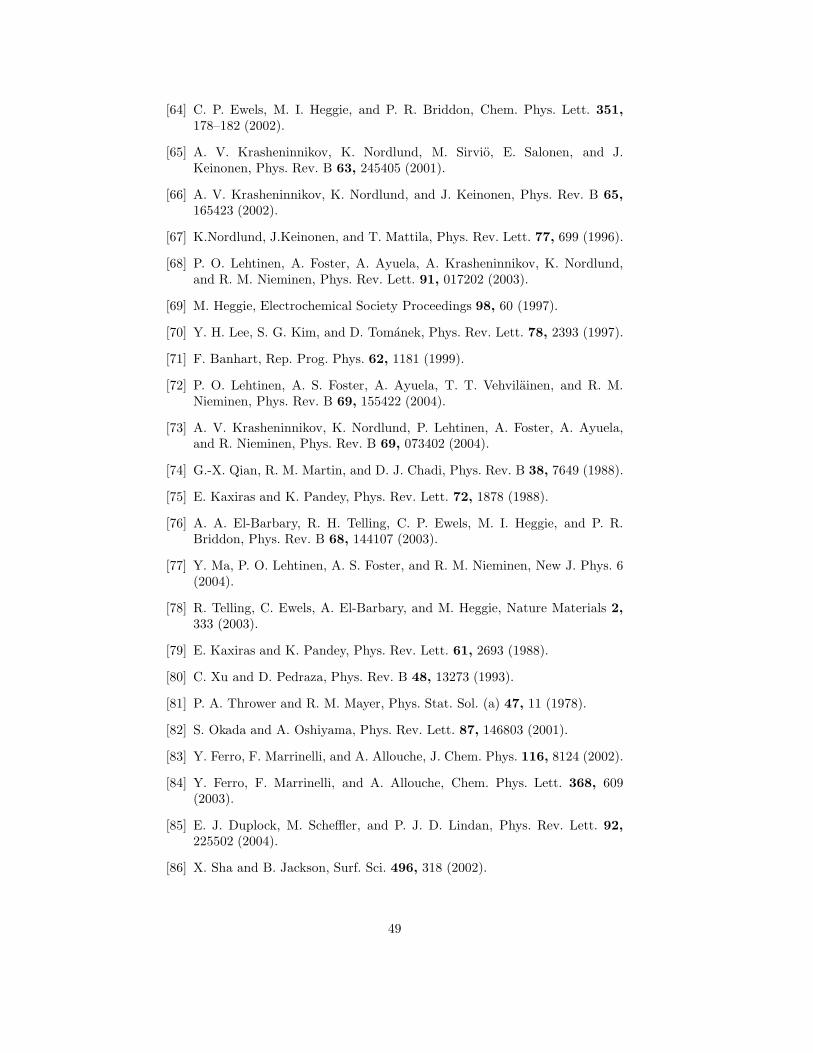
[64] C. P. Ewels, M. I. Heggie, and P. R. Briddon, Chem. Phys. Lett. 351,178–182 (2002).

[65] A. V. Krasheninnikov, K. Nordlund, M. Sirvio, E. Salonen, and J.Keinonen, Phys. Rev. B 63, 245405 (2001).

[66] A. V. Krasheninnikov, K. Nordlund, and J. Keinonen, Phys. Rev. B 65,165423 (2002).

[67] K.Nordlund, J.Keinonen, and T. Mattila, Phys. Rev. Lett. 77, 699 (1996).

[68] P. O. Lehtinen, A. Foster, A. Ayuela, A. Krasheninnikov, K. Nordlund,and R. M. Nieminen, Phys. Rev. Lett. 91, 017202 (2003).

[69] M. Heggie, Electrochemical Society Proceedings 98, 60 (1997).

[70] Y. H. Lee, S. G. Kim, and D. Tomanek, Phys. Rev. Lett. 78, 2393 (1997).

[71] F. Banhart, Rep. Prog. Phys. 62, 1181 (1999).

[72] P. O. Lehtinen, A. S. Foster, A. Ayuela, T. T. Vehvilainen, and R. M.Nieminen, Phys. Rev. B 69, 155422 (2004).

[73] A. V. Krasheninnikov, K. Nordlund, P. Lehtinen, A. Foster, A. Ayuela,and R. Nieminen, Phys. Rev. B 69, 073402 (2004).

[74] G.-X. Qian, R. M. Martin, and D. J. Chadi, Phys. Rev. B 38, 7649 (1988).

[75] E. Kaxiras and K. Pandey, Phys. Rev. Lett. 72, 1878 (1988).

[76] A. A. El-Barbary, R. H. Telling, C. P. Ewels, M. I. Heggie, and P. R.Briddon, Phys. Rev. B 68, 144107 (2003).

[77] Y. Ma, P. O. Lehtinen, A. S. Foster, and R. M. Nieminen, New J. Phys. 6(2004).

[78] R. Telling, C. Ewels, A. El-Barbary, and M. Heggie, Nature Materials 2,333 (2003).

[79] E. Kaxiras and K. Pandey, Phys. Rev. Lett. 61, 2693 (1988).

[80] C. Xu and D. Pedraza, Phys. Rev. B 48, 13273 (1993).

[81] P. A. Thrower and R. M. Mayer, Phys. Stat. Sol. (a) 47, 11 (1978).

[82] S. Okada and A. Oshiyama, Phys. Rev. Lett. 87, 146803 (2001).

[83] Y. Ferro, F. Marrinelli, and A. Allouche, J. Chem. Phys. 116, 8124 (2002).

[84] Y. Ferro, F. Marrinelli, and A. Allouche, Chem. Phys. Lett. 368, 609(2003).

[85] E. J. Duplock, M. Scheffler, and P. J. D. Lindan, Phys. Rev. Lett. 92,225502 (2004).

[86] X. Sha and B. Jackson, Surf. Sci. 496, 318 (2002).

49

[87] P. Ruffieux, O. Groning, P. Schwaller, L. Schlapbach, and P. Groning, Phys.Rev. Lett. 84, 4910 (2000).

[88] A. Hashimoto, K. Suenaga, A. Gloter, K. Urita, and S. Iijima, Nature 420,870 (2004).

[89] R. K. Pathria, Statistical Mechanics (Butterworth-Heinemann, Oxford,1996).

50