Magnetic Feedback Experiments on the m/n = 2/1 Tearing Mode inthe HBT-EP Tokamak

David Lawrence Nadle

Submitted in partial fulfillment of therequirements for the degree

of Doctor of Philosophyin the Graduate School of Arts and Sciences

COLUMBIA UNIVERSITY2000

© 1999David Lawrence Nadle

All Rights Reserved

ABSTRACTMagnetic Feedback Experiments on the m/n = 2/1 Tearing Mode in

the HBT-EP Tokamak

David Lawrence Nadle

This thesis reports the results of feedback experiments on the m/n = 2/1 tearing mode

in HBT-EP. The feedback algorithm is implemented in a digital-signal processing (DSP)

computer with an output sampling rate of 100 kHz. The algorithm produces control signals

by adjusting the gain and phase of a quadrature measurement of the 2/1 mode. Two high-

power amplifiers drive a two-phase set of saddle coils with small toroidal extent (12° per

phase) to produce a rotating resonant control perturbation. A normalized model of

nonlinear 2/1 mode behavior is described and used to compare simulated mode dynamics to

experimental data. A frequency-dependent stabilization of the mode amplitude is included in

the model and observed experimentally. Two magnetic and two optical quadrature mode

detection methods are compared. A novel technique using four poloidal Mirnov probes

located near the plasma surface is the best performer. The fields produced by the highly-

localized saddle coil set and the strength of its resonance with the 2/1 mode are determined

with a 2D numerical model. The phase instability, an exponential growth of a feedback

phase error away from negative feedback, is investigated and measured unstable periods

show excellent agreement with theoretical predictions. The feedback system can slowly

attenuate saturated 2/1 modes, but cannot prevent the growth of unsaturated modes. The

phase instability decreases phase accuracy as gain increases, limiting feedback performance.

i

Table of Contents

1 Introduction.................................................................................................................................11.1 Feedback Stabilization of the 2/1 Mode.............................................................................31.2 The HBT-EP Tokamak.........................................................................................................51.3 Feedback in HBT-EP ..........................................................................................................101.4 Major Results.........................................................................................................................11

2 The 2/1 Tearing Mode in HBT-EP.......................................................................................132.1 Tokamak Equilibrium..........................................................................................................132.2 MHD Stability.......................................................................................................................132.3 Plasma Resistivity and Magnetic Islands ...........................................................................142.4 Magnetic Island Growth Model .........................................................................................162.5 Island Rotation Model .........................................................................................................192.6 Normalized Magnetic Island Model ..................................................................................212.7 Estimating the Normalized Model Coefficients ..............................................................222.8 Simulating Dynamic 2/1 Mode Behavior .........................................................................262.9 Summary ................................................................................................................................27

3 Quadrature Detection Methods..............................................................................................283.1 Fourier-Analyzing Rogowski Coils ....................................................................................283.2 Shell-Mounted Probes .........................................................................................................323.3 X-ray Tomography...............................................................................................................393.4 Summary ................................................................................................................................43

4 Feedback Control Coils............................................................................................................444.1 Saddle-Flange Model............................................................................................................454.2 Saddle Perturbation Mode Spectrum ................................................................................474.3 Forces and Torques at the Rational Surface.....................................................................494.4 Feedback Model Conventions............................................................................................514.5 Summary ................................................................................................................................52

5 Phase Instability Measurements..............................................................................................545.1 Experimental Technique .....................................................................................................545.2 Observations .........................................................................................................................555.3 Phase-Flip Timescale ...........................................................................................................575.4 Results ....................................................................................................................................575.5 Summary ................................................................................................................................59

6 Feedback Experiments.............................................................................................................606.1 The Feedback Algorithm ....................................................................................................606.2 Feedback Simulation............................................................................................................606.3 Frequency-Domain Analysis...............................................................................................626.4 Observations .........................................................................................................................656.5 Summary ................................................................................................................................68

7 Conclusion .................................................................................................................................697.1 Summary of Results .............................................................................................................697.2 Discussion of Results...........................................................................................................707.3 Suggestions for Future Work..............................................................................................70

8 References ..................................................................................................................................72A DSP Hardware And Software .................................................................................................75

A.1 DSP Hardware ......................................................................................................................75

ii

A.2 SMP Feedback Algorithm...................................................................................................75A.3 DSP Isolation Network .......................................................................................................82A.4 Saddle Coil Power Amplifiers.............................................................................................85

Table of Figures

Figure 1-1. Plasma surface perturbation with m/n = 2/1 helicity.................................................3Figure 1-2. Eastern view of HBT-EP. ..............................................................................................6Figure 1-3. Toroidal cross section of the HBT-EP tokamak, detailing one toroidal field

(TF) coil, the ohmic heating (OH) coil set, the vertical field (VF) coil set,two conducting shells and positioners, the vacuum vessel, and parts of thesupport structure. ...........................................................................................................7

Figure 1-4. HBT-EP limiter................................................................................................................8Figure 1-5. Conducting shells in fully inserted and fully retracted positions. .............................8Figure 1-6. Top view of HBT-EP, detailing diagnostic, equilibrium coil, and 2/1 control

coil placement. ................................................................................................................9Figure 1-7. Schematic of tearing mode feedback system. ............................................................10Figure 2-1. Nested flux surfaces. .....................................................................................................13Figure 2-2. Magnetic island...............................................................................................................14Figure 2-3. Island growth rate vs. island size at different levels of feedback current. .............19Figure 2-4. Rise time model of growing m = 2 mode...................................................................23Figure 2-5. Island perturbation amplitude rise time vs. dimensionless model coefficient

g1. .....................................................................................................................................23Figure 2-6. Feedback/growth coefficient ratio vs. steady-state reduced b. The curve

maximum value is required to access any small b from a higher b on theright side of the hill. .....................................................................................................24

Figure 2-7. Rotation decay time vs. viscosity coefficient h1. The mode rotation decaysfrom Ω = 1.5 to Ω = 1.05. .........................................................................................25

Figure 2-8. Simulation of 2/1 mode response to a phase-flip discharge and comparisonto experiment. The phase flip occurs at 0.5 ms. The g3 = 0 trace is discussedin Section 5.2.1..............................................................................................................27

Figure 3-1. m = 2 Fourier-analyzing Rogowski coil. .....................................................................29Figure 3-2. Schematic diagram of one m = 2 Rogowski coil instrumentation circuit. .............30Figure 3-3. Rogowski feedback diagnostic detection of a growing m = 2 mode......................31Figure 3-4. Rogowski feedback diagnostic response to plasma and resonant magnetic

perturbation. The saddle coils are energized at 4 ms with ~250 A at 15 kHz(dashed trace). Diagnostic quadrature is lost between 4 and 4.4 ms. ...................32

Figure 3-5. View of shell-mounted probe (SMP) diagnostic installed in HBT-EP..................33Figure 3-6. Poloidal map of SMP fluctuations showing dominant m = 2 structure. ...............34Figure 3-7. Amplitude and phase evolution of m = 2 mode determined by SVD. ..................35Figure 3-8. Schematic diagram of one SMP feedback instrumentation circuit.........................36Figure 3-9. SMP feedback diagnostic response to a growing 2/1 mode. ..................................37Figure 3-10. SMP feedback diagnostic response to the same plasma and applied

perturbation as Figure 3-4...........................................................................................38Figure 3-11. SMP samples and amplitude and phase representations from a fifteen

channels SVD fit and the four channels SMP feedback diagnostic......................39

iii

Figure 3-12. Surface-tangential photodiode arrangement............................................................40Figure 3-13. Surface-tangential XRT diagnostic response to a growing 2/1 mode. ................41Figure 3-14. Unfiltered soft X-ray signal. .......................................................................................41Figure 3-15. Surface-normal photodiode arrangement. ...............................................................42Figure 3-16. Surface-normal XRT diagnostic response to a growing 2/1 mode. ....................42Figure 4-1. Top half of m = 2 saddle coil mounted over quartz insulator ring and

vacuum vessel flanges. .................................................................................................44Figure 4-2. Saddle coil set and stainless steel flange model with zero flange current. .............45Figure 4-3. Saddle coil set and stainless steel flange model with Iflange/Isaddle = 1.6...................46Figure 4-4. Br on q = 2 surface. Cosine and sine coil sets carry equal current..........................47Figure 4-5. Field fractions at the q = 2 surface of the first five n = ±1 modes by the

cosine coil set. Sine coil set fractions are similar, except B(2,-1) ~ 3.4%, dueto differences in orientation and toroidal spacing. ..................................................48

Figure 4-6. Field fraction of m = 2 components from cosine coil set. The 2/1 mode ishighlighted. The spectrum of the sine coil set is similar, with ~4% 2/1component and slightly different 2/n mode amplitudes. .......................................49

Figure 4-7. K×B forces on a helical current sheet at the zero phase, with equal current incosine and sine saddle coil sets...................................................................................50

Figure 4-8. Poloidal and toroidal torques (per ampere of saddle current) on a 4 kA/mhelical current sheet. Current is flowing only in the cosine coil set......................51

Figure 4-9. Cross-correlation of saddle-coil MHD pickup and mode diagnostics. Plotsshow correlation absolute value (normalized) vs. correlation phase in theband 5–25 kHz. ............................................................................................................52

Figure 5-1. Saddle coil currents, m = 2 signals, and phase difference signal of a phaseflip discharge. The perturbation phase flip (-180°) occurs just before 4.3 ms.The mode slows to re-lock with the regressed perturbation. The re-lockingperiod is within the shaded area.................................................................................55

Figure 5-2. Simulation of 2/1 mode response to a phase-flip discharge and comparisonto experiment. The phase flip occurs at 0.5 ms. Simulation g3 = 8,000. Thetrace with g3 = 0 shows the result of neglecting the effect of frequency-dependent inertial damping on mode amplitude. ....................................................56

Figure 5-3. Measured phase instability re-locking times vs. predicted time scales. ..................58Figure 6-1. Simulated 2/1 mode amplitude and frequency modification under ideal

feedback vs. constant feedback phase. The mode is initially at b = 1, Ω = 1at T = 0. G = 5. ............................................................................................................61

Figure 6-2. Simulated normalized amplitude and frequency values after feedback with10 µs latency, over a 1 ms period. The simulation demonstrates reducedcontrol over the feedback phase difference. G = 5. ...............................................62

Figure 6-3. Block diagram of the feedback loop transfer function. Frequencyconvolution of the output current and input field allow s-domain analysisof the feedback-produced force and torque.............................................................63

Figure 6-4. Frequency response of DSP feedback loop (δ = 0). As system frequencyincreases, mode attenuating force (ID) decreases, and mode acceleratingtorque (IQ) increases. ....................................................................................................64

Figure 6-5. Map of direct feedback current magnitude vs. frequency and feedback δ............65Figure 6-6. Tearing mode DSP feedback signals for an unsaturated mode. Feedback is

applied between 4.5 and 6.5 ms. ................................................................................66

iv

Figure 6-7 Tearing mode DSP feedback signals for a saturated mode. Feedback isapplied between 5 and 7 ms........................................................................................67

Figure 6-8. Variation of the feedback phase difference (∆Φ) and deviation of its meanfrom the programmed feedback phase difference (δ), vs. G . In this plotG ≡ <IA/B>. .................................................................................................................68

Figure 8-1. DSP output isolation circuit schematic diagram (G = 5). .......................................82Figure 8-2. DSP output isolator transfer functions. .....................................................................83Figure 8-3. DSP input isolation circuit schematic diagram (G = -1)..........................................83Figure 8-4. DSP input isolator transfer functions, including overvoltage protection

circuit..............................................................................................................................84Figure 8-5. DSP trigger isolation circuit schematic diagram........................................................84Figure 8-6. DSP input overvoltage protection circuit schematic diagram (G = 0.6)...............85

Table of Tables

Table 2-1. Measured and estimated experimental parameters used in simulations..................26Table 2-2. Estimated and theoretical values of model coefficients and values used in

simulations.....................................................................................................................26Table 4-1. Feedback phase convention...........................................................................................51Table 5-1. Phase instability measured model quantities and experimental results. ..................58

v

Acknowledgements

I have so many to thank for their support and assistance during my years at Columbia.

Thank you Eunjoo, for being the source of my joy. Thank you Dad, Maria Esperanza, and

Jeremy, for being such a loving and solid family. Thank you Mom, fifteen years free of this

Earth, for remaining with me in the form of tears. I dedicate this thesis to you.

Professors Michael Mauel and Jerry Navratil helm HBT-EP and navigate the fusion

research microcosm with awe-inspiring skill. Without their guidance I would have drowned.

Dean Robert Gross is a hero of mine, and that places me in good company. I am indebted

to him for his kindness and generosity.

Marlene Arbo and Lydia Argote hold the Applied Physics department together, and

while performing that miracle they have always made me feel loved and cared about

“upstairs.” I am grateful.

Nick Rivera is a man of extraordinary insight, intelligence, and wit. I wish I could eat

lunch with him every day for the rest of my life. Moe Cea is not a large man, but he leaves a

huge wake of laughter, warmth, and wisdom (and sometimes pump oil). I admire him

greatly. Estuardo Rodas never has a bad thing to say about anyone, even when they deserve

it. I have tried to follow his example with limited success. I value his friendship. Tom Ivers is

one of the most honorable and dedicated men I’ve ever known. Tom taught me everything I

know about working in a plasma physics lab.

The original HBT-EP gang, Ned Eisner, Andrea Garofalo, Raëd Kombargi, David

Maurer, Xiao Qingjun, and myself remain in close contact with each other. To make so

many friends in one place is a blessing. I think the original group influenced the present

culture of the lab, which chooses not closed ranks or rivalries but cooperates and embraces

strangers.

I’ve been fortunate to embrace several strangers as they entered Columbia. Ben Hall is a

genuine man and loyal friend. My thanks and best wishes to the present graduate students

and staff: Jimmy Andrello, Cory Cates, Hossein Dahi, Suparna Mukherjee, and Mikhail

Shilov. I hope that the works and creations I leave behind for you are a convenience and not

a curse.

1

1 Introduction“The energy produced by the atom is a very poor kind of thing. Anyone

who expects a source of power from the transformation of these atoms istalking moonshine.”—Lord Ernest Rutherford (Cerf and Navasky 1998).

Lord Rutherford is famous for inferring the nucleus of the gold atom, for predicting the

existence of the neutron and of “diplogen,” better known as deuterium (Wilson 1983), for

receiving the Nobel Prize in chemistry, and for making this prediction. Just a few years later

it would be known that nuclear fission is a terrific source of power. As the story goes, Leo

Szilard conceived the nuclear chain reaction after reading Rutherford’s quote in the London

Times (Lanouette 1992). Had Lord Rutherford added to his gaffe the paraleipsis, “not to

mention fusing them,” he would have been more on target. The development of nuclear

fusion power has been a slow and punctuated one.

Nuclear fusion inspired at least one Rutherford-like misstep when in 1942 Teller and

Konopinsky calculated that the fusion process was impossible (Gross 1984). They later

corrected their error, and by 1950 secret fusion energy research programs had been initiated

in the US, UK, and USSR. By 1958 it was mutually agreed that fusion energy production

would be very difficult, and the research was declassified. Despite the difficulties, fusion

research has progressed greatly in the last forty years, and most of the progress has been

made with one particular plasma confinement scheme, the tokamak.

The tokamak is a toroidal magnetic plasma confinement system. The plasma is confined

by a magnetic field to keep it from contacting the walls and material surfaces inside the

toroidal vacuum chamber where the discharge is formed. As long as such contact is

prevented, the plasma can be heated to the millions of degrees required for thermonuclear

fusion. A strong toroidal magnetic field forces the plasma ions and electrons into orbits

2

smaller than the minor radius of the chamber, but a poloidal magnetic field is necessary to

push against the fluid plasma pressure. In a tokamak the poloidal field is generated by the

plasma itself, as it carries a large toroidal current.

Fusion is moving closer to viability as a power source. The JET tokamak has reported

16.1 MW peak fusion power, with a fusion power to input power ratio Q > 0.6 (Gibson et al.

1998). If it ever was, talking about fusion power is no longer talking moonshine. Challenges

do remain, and chief among them is understanding and controlling the plasma behavior that

results in a major disruption, a rapid loss of the plasma’s confined thermal energy. The

precursor to disruptions in a tokamak is the m/n = 2/1 tearing mode instability. The tearing

instability takes its name from the action of the magnetic field lines inside the plasma. Field

lines near the mode-resonant surface in a resistive plasma tear and reconnect in different

topologies, creating threads of locally-closed flux surfaces called magnetic islands. The poloidal

mode number m and the toroidal mode number n describe a single helical mode of the

instability’s structure. The 2/1 mode is the lowest and largest mode of the instability.

Experimental studies on suppressing the 2/1 tearing mode using feedback magnetic fields

began in the 1970s, culminating in the late 1980s with a successful stabilization experiment in

the DITE tokamak (Morris et al. 1990).

This thesis presents the 2/1 feedback experiments in the HBT-EP tokamak. This

introductory chapter provides a summary of prior work in other tokamaks, an overview of

the HBT-EP tokamak and the focus of our feedback experiments, and a list of our major

results. The remaining chapters of this thesis present the theory, major experimental

equipment, and results of the feedback experiments in HBT-EP. The theory of 2/1 tearing

mode feedback is reviewed and discussed in Chapter 2. Chapter 3 contains a comparison of

the diagnostics used to obtain the best measurement of the m = 2 mode amplitude and

3

phase, for generating feedback signals. Chapter 4 presents the 2/1 control perturbation coil

set, with an analysis of its efficiency in producing resonant forces and torques. Investigations

of the feedback phase instability, the exponential growth of a small error in feedback phase

away from negative feedback, are discussed in Chapter 5. The feedback experiments and

results are in Chapter 6. Chapter 7 contains a summary and discussion of the results, and

suggestions for future work. Finally, Appendix A describes some of the hardware and

software used to perform the experiments.

1.1 Feedback Stabilization of the 2/1 ModeDisruptions in tokamaks are associated with the growth of the 2/1 tearing mode (Figure

1-1) and may result from destabilization of other helical plasma modes (Waddell et al. 1978)

or from island contact with a material surface (Sykes and Wesson 1980). Resistive MHD

instabilities like the 2/1 tearing mode grow on a longer time scale (milliseconds in HBT-EP)

than ideal MHD instabilities (microseconds). The slower growth rate of tearing modes

allows for some form of active stabilization to be employed to control them.

Figure 1-1. Plasma surface perturbation with m/n = 2/1 helicity.

Islands in a tokamak rotate due to diamagnetic forces and toroidal momentum imparted

to the plasma by external means, such as neutral beam heating. A rotating magnetic island

structure produces magnetic field oscillations at a multiple of its rotation frequency. The

4

island structure also perturbs the radiation profile of the plasma, so optical diagnostics may

be used to provide information about the tearing instability. The phase and amplitude of the

tearing mode are measured in real time to provide an input signal to a feedback loop.

An external magnetic perturbation, resonant with the mode being controlled by sharing

the same helicity (m/n ratio), can be used to apply stabilizing forces or torques or both.

Applying a constant perturbation will ultimately fail to stabilize the mode, because the mode

will flip its phase so that the perturbation becomes destabilizing (Monticello, White, and

Rosenbluth 1978). This is the phase instability. Feedback phase control is used to maintain a

stabilizing perturbation.

The predictions of tearing mode theory and the results of past experiments point to the

challenges facing tearing mode feedback, and form the basis for experiments in HBT-EP.

The primary challenges are technical: limitations in small-amplitude mode detection, mode

diagnostic error due to the applied control fields, limitations of loop gain and bandwidth,

and phase control inaccuracy. The physics challenges include the phase instability, the

influence of core thermal collapses on the instability drive, and the possible excitation of

modes other than the one under control.

Feedback experiments on the m = 2 mode in the ATC tokamak identified two problems:

coupling of the control perturbation into the feedback detector signal, and using external

magnetic diagnostics to detect a small-amplitude island. Distortion of the mode diagnostic

signals under feedback made the amplitude control data “difficult to evaluate” (Bol et al.

1975). When the mode was small and localized to its resonant surface, it had “no detectable

magnetic manifestation outside the plasma column.” The maximum loop gain in ATC was

“unsatisfactory” when using external magnetic probes to detect the mode. Loop gain is the

ratio of the rational-surface magnitude of the applied control perturbation to the rational-

5

surface magnitude of the magnetic island perturbation. A convenient definition of loop gain

for experimental work substitutes the control coil current for the control perturbation

amplitude. The experimental definition of loop gain has the symbol G in this thesis; it is not

to be confused with the Rutherford growth coefficient in Chapter 2.

The TO-1 tokamak demonstrated a feedback-phase dependent decrease or increase in

m = 2 mode amplitude. Amplitude reduction of 65% was accompanied by increases in

plasma electron density and temperature (Arsenin et al. 1978). Control perturbations were

produced with a single pair of windings, launching a standing wave in the plasma. With a

rotating 2/1 mode present the standing wave can be represented as two waves rotating in

opposite directions, one of which is resonant with the 2/1 mode. Like ATC, mode

diagnostic accuracy in TO-1 was limited by coupling of the control perturbation.

The successful application of feedback in the DITE tokamak produced a 70% reduction

in mode amplitude. Mode reduction was accompanied by an increase in plasma density and a

delay in the onset of major disruptions (Morris et al. 1990). Stabilization was limited by rapid

increases in the instability drive due to sawtooth-like collapses of the plasma core

temperature, and by limited amplifier power. A disruption-causing sawtooth triggered a rapid

increase in the width of the m = 2 island, beyond the maximum width that can be controlled

at maximum feedback loop gain.

The focus of feedback experiments in HBT-EP and their distinguishing characteristics

are discussed below, following an introduction to HBT-EP.

1.2 The HBT-EP TokamakHBT-EP (Figure 1-2) is an ohmically-heated tokamak, the plasma current being induced

by a primary transformer winding in the center of the torus. The hoop force of the plasma

current is opposed by a vertical magnetic field to stabilize the plasma major radius.

6

Figure 1-2. Eastern view of HBT-EP.

A toroidal cross section of HBT-EP detailing the equilibrium field coils is shown in

Figure 1-3. The toroidal field (TF) is generated by twenty coils and powered by a 40 mF

capacitor bank. The bank is typically charged to 6 kV and produces 0.35 T at R = 92 cm.

The ohmic heating (OH) system in HBT-EP differs from most other tokamaks. It was

designed to induce a fast rise in the plasma current, faster than the plasma resistive diffusion

or “soak through” time, so the current rises before the plasma temperature rises (Vijaya

Sankar et al. 1993). 20 kA of plasma current is generated by two high-voltage banks in the

first 100 µs, and an additional electrolytic bank extends the plasma current ramp for 3 ms.

The vertical field (VF), typically 4–5 mT, is programmed by adjusting capacitor bank

voltages to maintain the desired plasma major radius.

7

Figure 1-3. Toroidal cross section of the HBT-EP tokamak, detailing one toroidalfield (TF) coil, the ohmic heating (OH) coil set, the vertical field (VF) coil set, twoconducting shells and positioners, the vacuum vessel, and parts of the supportstructure.

Plasma minor radius is defined by two sets of stainless steel limiter blades on opposite

sides of the vessel, in the toroidal gap between conducting wall segments (Figure 1-4). They

are positioned to prevent the hot plasma from contacting the conducting wall surfaces.

8

Figure 1-4. HBT-EP limiter.

HBT-EP was constructed to investigate

active and passive stabilization of performance-

limiting MHD instabilities. Ideal MHD

instabilities, the fastest growing class, are

stabilized by eddy currents induced in a close-

fitting, segmented conducting wall. The wall

segments (or shells) are nickel-coated

aluminum, 1 cm thick. A unique capability of

HBT-EP is that each of the twenty shells can be manually positioned along an 8 cm range in

minor radius to vary the amount of passive wall stabilization (Figure 1-5). For the active

feedback stabilization experiments in this thesis the maximum amount of passive

stabilization was desired, and the shells were kept fully inserted.

Figure 1-6 presents a top view of HBT-EP, detailing the placement of the major

diagnostics and the 2/1 control coils. The control coils and some magnetic diagnostics are

mounted on quartz insulating sections for superior response. The control coils and some of

the important diagnostics for feedback experiments are covered in depth below. Other

major diagnostics provide information about the plasma discharge. The soft x-ray (SXR) fan

Figure 1-5. Conducting shells in fullyinserted and fully retracted positions.

9

array measures the plasma radiation profile. Thomson scattering uses the scattering of laser

light to measure plasma temperature. A microwave interferometer measures plasma density.

A spectrometer looks at the radiation from plasma impurities to measure plasma rotation. A

Mach probe measures ion flow.

m = 2

Figure 1-6. Top view of HBT-EP, detailing diagnostic, equilibrium coil, and 2/1control coil placement.

The plasma major radius R0 is derived by a polynomial fit to a function of the

measurements with a θcos Rogowski coil (see Section 3.1 for a discussion of Rogowski

coils), with corrections from measurements of the total plasma current and equilibrium field

10

coil currents. The fitting procedure in HBT-EP is described by Gates (1993). The

equilibrium density is derived from a microwave interferometer line measurement and the

estimated chord length, based on measured R0 and the limiter position. Rogowski coils are

attached to the saddle coil winding circuits to measure Isaddle. The minor radius rs of the

mode-resonant surface is estimated at 0.09 m. This estimate is in agreement with soft X-ray

and Mach probe measurements.

1.3 Feedback in HBT-EPThe HBT-EP feedback experiments employ a phase-shifting algorithm implemented in a

digital signal-processing (DSP) computer to produce control signals. A schematic of the

basic technique is shown in Figure 1-7. The aim is for the mode diagnostics to provide a

measurement of the 2/1 mode while rejecting pickup from the applied control field. The

algorithm produces a quadrature representation (see Chapter 3) of the 2/1 mode and

produces a phase-shifted output signal. The output signal is amplified and run through the

control windings, producing a resonant quadrature magnetic field, which when properly

phased, opposes the field produced by the 2/1 mode.

Figure 1-7. Schematic of tearing mode feedback system.

Two characteristics of the feedback system limit feedback performance in HBT-EP. The

noise rejection of the mode diagnostics is finite, and this limits the smallest mode amplitude

11

that can be accurately measured. The DSP computer has a finite operating speed, and the

time delay between an input sample and output response causes feedback phase error.

To achieve a better understanding of the use and limitations of magnetic feedback on the

2/1 tearing mode, the feedback experiments in HBT focus on the following questions.

• How does optical detection of mode phase and amplitude compare to magnetic

detection for feedback stabilization of the 2/1 tearing mode? The criteria for comparison

are those that affect the complexity of the feedback system: number of channels

required, measurement accuracy, noise level, and small-amplitude detection threshold.

• Do our observations of the phase instability match the growth rate predicted by theory?

• What constraints does the phase instability place on feedback in HBT-EP? DITE

reported the phase instability to be experimentally “weak,” but HBT-EP’s phase

instability time scale (100–300 µs) is faster than DITE’s (300–3,000 µs).

• Can HBT-EP’s m = 2 fluctuation amplitude be reduced with two-phase rotating

magnetic perturbations, applied with highly-localized modular saddle coils? The single-

phase external control windings in ATC covered 70 toroidal degrees. The single-phase

internal control windings in TO-1 covered 90 toroidal degrees. Each phase of the two-

phase internal control windings in DITE covered 40 toroidal degrees (Morris et al.

1989). In contrast, one phase of the two-phase external control windings in HBT-EP

covers just 12 toroidal degrees. Decreased coil area and proximity requirements are

favorable in fusion reactor designs containing neutron blankets and many access ports.

1.4 Major ResultsWe were successful in addressing the four questions outlined above. Major results are

listed below:

12

• Optical mode detection was found to be inferior to magnetic mode detection at similar

levels of system complexity.

• Our experimental observations of the phase instability time scale show excellent

agreement with theoretical predictions made with measured plasma characteristics.

• The phase instability limits feedback performance in HBT-EP by limiting the feedback

loop’s ability to maintain the programmed phase.

• Reduction of the 2/1 mode amplitude with feedback was modest. The highly-localized

control coil geometry reduces total available loop gain.

13

2 The 2/1 Tearing Mode in HBT-EPThe tearing mode is a form of the kink instability, which is driven by plasma current

flowing parallel to magnetic field lines. A kink or bend in a toroidal plasma current is

stabilizing, but the effect is minimized when the helical pitch of the magnetic field lines (the

ratio of toroidal circuits to poloidal circuits) is a rational number at a minor radius just

outside the plasma surface.

2.1 Tokamak EquilibriumThe condition for plasma equilibrium is that the total forces on

the plasma vanish everywhere. This condition is p∇=×BJ . The

implication of this condition is that a toroidal equilibrium requires

a toroidal current and poloidal current to balance the plasma

pressure. In the ideal axisymmetric MHD equilibrium the magnetic

field lines lie on nested toroidal flux surfaces of constant pressure (Figure 2-1).

2.2 MHD StabilityThe stability of a tokamak equilibrium may be examined using the energy principle, a

variational formulation of the normal modes of the linearized MHD equations (Bernstein et

al. 1958). The energy principle is embodied in a variational equation for the change in

potential energy of a perturbation of the plasma. If the change in potential energy

∫ ⋅−= dVW Fî21δ is negative for any perturbation with displacement ξξ and force F(ξξ), that

perturbation leads to a growing instability. The integral is expanded in powers of the inverse

toroidal aspect ratio ε ≡ a/R0, and the zero and first order terms are stabilizing. The second

order term describes the kink instability and may be written as

Figure 2-1. Nestedflux surfaces.

14

drrdr

dJ

m

nqBRW

br

∫

−+=

0

22

102

2 1 ξπδ φθB (2.1)

for the mode m/n, where ( )01 BîB ××∇= is the perturbed magnetic field and the limit of

integration rb is the radius of a perfectly conducting wall surrounding the plasma. If a

vacuum region exists between the plasma and the wall (plasma minor radius a < rb), ξξ may be

nonzero at the plasma surface and the second term can be destabilizing when the plasma

current gradient is large. The quantity q (a radial function of the helical pitch of the magnetic

field lines) is named the kink safety factor because when the plasma surface value qa > m/n

the second term is positive and the kink mode is stabilized. The ideal m/n mode is called an

external mode (for m > 1) because it grows when the rational q surface lies outside the

plasma.

2.3 Plasma Resistivity and Magnetic IslandsThe effects of plasma resistivity on plasma equilibrium are

negligible everywhere except inside a small layer surrounding a

mode-rational flux surface inside the plasma called the resistive layer

(Furth, Killeen, and Rosenbluth 1963), also called the boundary

layer or singular layer. Inside this layer plasma resistivity frees the

nested field lines of ideal MHD to tear and to reconnect with field lines on other surfaces.

When tearing is present, the intersections of field lines with a toroidal section of the plasma

trace out a pattern of locally closed flux surfaces called magnetic islands, separated from the

rest of the plasma by a multiply connected surface called the separatrix (Figure 2-2). The

magnetic center of an island is often called an O-point, and the points of connection of a

separatrix are known as X-points.

The width of the 2/1 magnetic island is given by

Figure 2-2. Magneticisland.

15

( )[ ]

sr

s

qB

rqW

′=

θ

ψ~4 (2.2)

where ψ~ is the perturbed helical flux ( ψ~1 ∇=B ) and q = m/n at the rational surface rs.

Outside the resistive layer, the flux surfaces obey the infinite-conductivity equation

(Furth, Killeen and Rosenbluth 1963; Furth, Rutherford, and Selberg 1973), which is given

in cylindrical coordinates as

0~~

12

=

+−

−

dr

dFH

dr

dF

F

g

dr

dH

dr

d ψψ(2.3)

where Bk ⋅=F , ( )2223 mrkrH += , and g is a rather involved function of B, k, m, r, and

the pressure gradient. At the rational surface F = 0, therefore (2.3) is solved in regions

0 < r < rs and r > rs and the solutions are matched at rs . The radial derivative of ψ~ is usually

discontinuous, and the relative size of the discontinuity is represented by

( )2

2~

~ Wr

Wr

s

s

W+

−

′=∆′ψψ

(2.4)

The equilibrium is unstable to tearing modes when ∆´ > 0. The growth of a tearing mode is

observed as an increase in the width of its associated islands. ∆´ is typically a monotonically

decreasing function of W.

When the island width is smaller than the width of the resistive layer, the tearing mode

grows fastest. It is slowed from the ideal mode growth rate by the time it takes for magnetic

field lines to tear and reconnect. When the island is wider than the resistive layer, nonlinear

eddy currents grow in response to the perturbed field. The nonlinear currents oppose the

perturbed mode current and further slow the growth rate of the tearing mode to the resistive

16

skin time ( ηµτ 02aR ≡ ), the timescale of the diffusion of magnetic field lines through the

resistive plasma (Rutherford 1973). The skin time in HBT-EP is ~30 ms.

A second nonlinear reduction in the tearing mode growth rate comes into effect when

the island width is comparable to the shear length (1/q´) at the rational surface (White 1986).

External forces and geometry dominate mode behavior in this regime, and it becomes

possible for the island to reach a size where the growth rate becomes zero. This is known as

the saturated island size, and ( ) 0=∆′ satW . The saturated island width in HBT-EP is

estimated at ~3 cm.

2.4 Magnetic Island Growth ModelThe growth rate of the tearing mode magnetic island in the Rutherford (nonlinear)

regime is primarily determined by ∆´ and skin time, as 0µη∆′=GdtdW . The model

described here is adapted from a derivation which includes neoclassical effects such as

bootstrap current and parallel viscosity (Smolyakov et al. 1995). Bootstrap current is

negligible in HBT-EP’s plasmas, and the model is not expected to fit HBT-EP’s mode

behavior precisely. The model includes the transient, frequency-dependent mode damping

required to explain HBT-EP’s results (Navratil et al. 1998). Measured or estimated values for

all the parameters used in the model are given in Section 2.7.

2.4.1 The Feedback Control Term

When a resonant magnetic perturbation produced with external windings interacts with

the tearing mode, the boundary conditions for the outer solution of ψ~ are modified, which

modifies ∆´. The effect of feedback on the island width can therefore be written as its

contribution to the total ∆´ (Monticello and White 1980). The feedback coil ∆´ used here is

17

specific for the 2/1 mode and makes use of the “tenuous plasma” approximation (Nave and

Wesson 1990), which assumes little plasma current outside the rational surface.

( )( ) ∆Φ=∆′ cos~ 2

0

b

sAcoil r

r

t

tI

ψµ

(2.5)

The feedback control current IA(t) is modeled as a single helical current at radius rb. A

current scaling factor relating the HBT-EP control winding geometry to an ideal helical

current is presented in Section 4.2. The feedback coil ∆´ is most stabilizing when the phase

difference (∆Φ) between the coil perturbation and the mode perturbed flux (ψ~ ) is 180º. The

estimated maximum value of ∆´coil in HBT-EP is on the order of ±0.01 m-1.

2.4.2 The Inertial Damping Term

The frequency dependent component of island stabilization in HBT-EP behaves

similarly to the predicted effect of ion inertia on island growth. On the island separatrix the

effect of plasma inertia must be added to Rutherford theory to compute island kinetic energy

(Edery et al. 1983). Plasma inertia affects island growth through an ion polarization current

whose contribution to ∆´ is proportional to W-3 (Wilson et al. 1996). The inertial damping

contribution to ∆´ in this model is proportional to the square of the difference between the

mode frequency and its natural rotation frequency (ω0). Other proportions are possible. In

HBT-EP the modes are observed to rotate at the electron diamagnetic drift frequency

( 20 aeBTee =∗ω ). This frequency is approximately 10 kHz in HBT-EP. The inertial

damping term is given by

( )3

20

22016

Wvqr

RG

As

ωω −

′

−=∆′ ΓΓ (2.6)

18

where the Alfvén velocity iA mnBv 000 µ= . The Alfvén velocity in HBT-EP is

approximately 2×106 m/s. Smolyakov (1995) gives GΓ ~ 1.06. The inertial damping term can

attain the same magnitude as the feedback control term with a few percent frequency

deviation from ω0.

2.4.3 The Island Width Equation

With the important terms (2.5) and (2.6) elaborated, we can now write the approximate

island width equation for HBT-EP plasmas.

( )Γ∆′+∆′+∆′= coilGdt

dW

0µη

(2.7)

Theoretical estimates of coefficient G can range from 0.43 (Fitzpatrick and Hender 1991) to

1.22 (Hegna 1998). This variation is small compared to uncertainties in estimating ∆´.

2.4.4 Feedback Attenuation of Island Width

With constant negative feedback on a saturated mode rotating at the natural frequency,

the Rutherford growth term and the inertial damping term are zero. Substituting (2.5) into

this reduced island width equation, with sr rmB ψ~~ ≈ and m = 2, gives

2~2

br

A

W rB

I

dt

dW

sat

η−≅ (2.8)

This is the fastest possible rate of island width reduction under ideal feedback. If increases in

the instability drive cause the island to grow faster than this rate ( 0>∆′+∆′ coil ), control of

the island width is lost. The initial attenuation rate using typical HBT-EP parameters is on

the order of 0.3 mm/ms.

19

Figure 2-3 plots island growth rate versus island size at different levels of feedback

control current. Neglecting inertial damping, (2.7) is solved for the minimum current (IC)

required to reduce the island size to zero.

( )0216

22

∆′

= s

s

sat

s

bsC r

r

W

r

rSII

π(2.9)

02 µπ θBrI ss ≡ is the toroidal plasma current enclosed by the q = 2 surface. qqrS s ′≡ is a

dimensionless magnetic shear coefficient. This model gives a value for HBT-EP of ~1.6 kA.

Available current is limited to less than 30 A. According to (2.9) direct island width

reduction in HBT-EP is limited to a small fraction of the saturated island width.

0.1 0.2 0.3 0.4 0.5 0.6 0.7 0.8 0.9 1-80

-60

-40

-20

0

20

40

60

80

dt (

m/s

)

W/Wsat

IA = IC

IA = IC/2

IA = 0

Figure 2-3. Island growth rate vs. island size at different levels of feedback current.

2.5 Island Rotation ModelThe balance of electromagnetic torques and viscous damping forces determines the

deviation of island rotation from its natural frequency. The angular acceleration of the island

is determined from these forces and the island moment of inertia. Two different models for

20

the island moment of inertia exist in the literature. Lazzaro and Nave (1988) treat the

moment of inertia as a constant fraction of the plasma moment, while Smolyakov et al.

(1995) treat it as a function of island width. The experimental range of island width in HBT-

EP is not large enough to distinguish between these two models.

Important electromagnetic contributions to island rotation include drag torque from

eddy currents in the conducting wall, and torque from the quadrature phase of the feedback

control perturbation. The electromagnetic terms in the mode frequency equation are

modeled in the same manner as in the island width equation, except that they use the

imaginary part or quadrature phase of the stability indices.

2.5.1 Wall Drag

Eddy currents flowing in the conducting wall in response to the mode-perturbed field

produce a torque opposing island rotation. For a continuous wall, the time scale for the

dissipation of the eddy currents is related to the skin time of the wall, mdw 20σδµτ ≅ ,

where the wall has thickness δ, radius d and conductivity σ (Fitzpatrick 1993). The wall time

in HBT-EP is on the order of 10 ms. Wall drag torque is very small when wωτ >> 1, as it is

for 10 kHz 2/1 modes in HBT-EP, so the drag term can be neglected in the island rotation

equation.

2.5.2 Feedback Quadrature Torque

The feedback quadrature ∆´ is similar to the direct term (2.5), except that the sine phase

is used.

( )( ) ∆Φ−=∆′ sin~ 2

0,

b

sAcoilq r

r

t

tI

ψµ

(2.10)

The feedback quadrature ∆´ is approximately ±0.01 m-1 in HBT-EP.

21

2.5.3 The Island Rotation Equation

The island rotation equation obtains from conservation of momentum ( Γ=ω&I ). In this

model the island moment of inertia I depends on the island width. This model also includes

a term which behaves like a viscous flow damping torque. The observed viscosity (µα) is

termed anomalous, because it is much larger than the classical value of the plasma viscosity

due to ion-ion collisions. The first term slows rotation of a growing island and increases

rotation of a suppressed island.

( ) ( ) ( ) ( )coilqAs

oi

a vR

WrqG

Wnm

G

t

W

Wt ,2

40

32

200216

61 ∆′′

−

+

∂∂−−=−

∂∂ τµµωωωω (2.11)

The wall drag is neglected. Coefficients Gµ ≈ 2.82 and Gτ ≈ 1.22.

The conservation of the toroidal momentum in the model of the rotating 2/1 island

indicates that decreasing mode amplitude ( 0<W& ) is accompanied by an increase in ω& when

0ωω > . This is distinct from the phase instability and cannot be avoided by perfect negative

feedback, because the quadrature feedback term does not contribute to ω& when π=∆Φ .

2.6 Normalized Magnetic Island ModelThe equations governing magnetic island evolution in HBT-EP can be expressed in a

better form for analyzing experimental data by normalizing the island width to its saturated

value and the island rotation frequency to its natural frequency. Island width and perturbed

flux are recast as expressions for a dimensionless .

~~satr BBb ≡ . Rotation frequency is

replaced with 0ωω≡Ω . Rutherford growth is modeled linear in island width, g1 at W = 0,

zero at W = Wsat. The island width equation (2.7) becomes

( ) ( )b

gb

tIgbbg

dt

db A2

321

1cos

)(1

−Ω−∆Φ+−= (2.12)

22

The Rutherford growth coefficient ( )

∆′=sat

s

M

s

W

rrGg

τ0

21 , where ηµτ 02

sM r≡ is the

magnetic diffusion time. The feedback coupling coefficient 32

2

64

=

sat

s

b

s

Ms W

r

r

r

SI

Gg

τπ

, and

the inertial damping coefficient 44

0

2

023

8

= Γ

sat

s

sA

s

M W

r

r

R

v

r

S

GGg

ωτ

.

The island rotation equation (2.11) becomes

( ) ( ) ∆Φ+

∂∂+−Ω−=

∂Ω∂

sin2

1121 tIbh

t

bh

bt A (2.13)

The viscous damping coefficient νµ τGh 61 = , where αν µρτ 20 satW≡ is the saturated island

viscous rotational relaxation time. The quadrature feedback coupling coefficient

=

s

sats

b

s

s

A

s r

W

R

r

r

r

r

v

I

SGh

4

0

2

02

2

2

2ω

π τ . Wall drag is neglected. The saturated island width,

natural rotation frequency, and equilibrium plasma parameters are held constant over the

time scale with which (2.12) and (2.13) are applied.

2.7 Estimating the Normalized Model CoefficientsEstimating the values of the normalized model coefficients is complicated by the fact

that some parameters are difficult to measure, and some coefficients are sensitive to the

fourth or fifth power of underlying plasma parameters. An experimental estimate for g1

obtains from measuring the rise time (from 10% to 90% of the saturated amplitude) of

naturally growing modes (Figure 2-4).

23

Figure 2-4. Rise time model of growing m = 2 mode.

The rise time in HBT-EP is usually 400–900 µs. The island growth coefficient g1 is less

sensitive to rise time in this range (Figure 2-5), and g1 ~ 1000 Hz.

Figure 2-5. Island perturbation amplitude rise time vs. dimensionless modelcoefficient g 1.

Estimating the magnitude of g2 experimentally is complicated by the effect of inertial

damping, but an upper limit is estimable by setting 0=dtdb in (2.13) and plotting the ratio

of coefficients for a given steady-state reduced value of b under ideal negative feedback

(Figure 2-6). Transients make it difficult to measure a steady-state reduction in b, but it is

24

observed that the mode is not completely suppressed. Therefore, a maximum helical control

current (IA) of approximately 24 A yields g2 < 6 C-1.

Figure 2-6. Feedback/growth coefficient ratio vs. steady-state reduced b. The curvemaximum value is required to access any small b from a higher b on the right side ofthe hill.

The viscosity coefficient h1 is estimated by observing the relaxation of mode rotation

after unlocking from a perturbation above the natural rotation frequency. Ivers et al. (1996)

reported a relaxation time τν in HBT-EP of 500 µs from a point 4 kHz above the natural

frequency, but relaxation within a rotation cycle ( 10 <ωτν ) has also been observed (Navratil

et al. 1998). The viscosity coefficient h1 is sensitive to relaxation time in this range (Figure

2-7). The estimated range for h1 is 5,000–20,000 Hz.

25

Figure 2-7. Rotation decay time vs. viscosity coefficient h1. The mode rotation decaysfrom ΩΩ = 1.5 to ΩΩ = 1.05.

The feedback quadrature coefficient h2 and the direct coefficient g2 have the same source

∆′, and some manipulation gives an estimate for the ratio

44

002

22

2

2

232

=

s

sats

s

MA

r

W

R

r

r

v

G

SG

g

h

ωττ (2.14)

The ratio is approximately 700 in HBT-EP.

The inertial damping coefficient g3 and hard-to-measure plasma parameters like viscosity

and magnetic shear are estimated by modeling island growth and matching to observed

mode amplitude. The mode suppression due to fast changes in mode rotation frequency

away from the natural frequency, which is attributed to inertial damping, is a transient effect.

In the tearing mode model this transience is produced by restoring torques dependent on

island width. This coupling of the island width and rotation equations makes it difficult to

isolate g3 experimentally. Simulations of island growth presented in the following section are

compared to data from a phase-instability test discharge like those discussed in Chapter 5.

Table 2-1 contains a list of the plasma parameters used to estimate the simulation

coefficients.

26

Table 2-1. Measured and estimated experimental parameters used in simulations.

∆´(0) ≈ 120 m-1 η ≈ 7.2×10-7 Ω-m Wsat. ≈ 2.5 cm 1/q’ ≈ 3 mm

G = 0.61 GΓ = 1.06 Gµ = 2.82 Gτ = 1.22

µα ≈ 6×10-9 kg/m-s B0 = 0.33 T Bθ ≈ 16 mT ρ0 ≈ 2×10-8 kg/m3

νA ≈ 2×106 m/s R0 ≈ 94 cm rb = 31 cm rs ≈ 9 cm

f0 = 8 kHz S ≈ 15 τM ≈ 14 ms Is ≈ 7.2 kA

Estimated and theoretical values for the normalized model coefficients are listed in Table

2-2 along with the values used in simulations. The discrepancy between theoretical and

simulation values of g3 is not unexpected, for reasons outlined above.

Table 2-2. Estimated and theoretical values of model coefficients and values used insimulations.

experiment model simulation experiment model simulationg1 ~1,000 ~3000 2,000 h1 5E3–20E3 1.4E12 µα 8,000g2 <6 ~0.3 1 h2 <3500 ~200 600g3 ~12 8,000

2.8 Simulating Dynamic 2/1 Mode BehaviorA comparison of data from a phase instability test discharge and a dynamic simulation of

the normalized model with coefficients from Table 2-2 show good agreement, especially

with mode frequency and phase (Figure 2-8). The simulation value of g3 (8,000) produces a

better fit to mode amplitude evolution than simulation with g3 = 0, and does not affect the

fit to mode rotation dynamics. Other simulations of phase instability and feedback dynamics

using the normalized model are presented in Chapters 5 and 6.

27

Figure 2-8. Simulation of 2/1 mode response to a phase-flip discharge andcomparison to experiment. The phase flip occurs at 0.5 ms. The g 3 = 0 trace isdiscussed in Section 5.2.1.

2.9 SummaryTearing modes are associated with the formation of magnetic islands at the mode

rational surface. The modes grow exponentially in time when small, then linearly in what is

confusingly called the nonlinear or Rutherford regime. With further growth, the island

eventually saturates, reaching its maximum width. Tearing mode growth and rotation models

are described, taking into account inertial damping of island width and viscous damping of

island rotation. A normalized version of the model is offered to facilitate its application to

experiments. Simulations using the normalized model show good agreement with observed

dynamics of the 2/1 mode in phase instability test discharges.

28

3 Quadrature Detection MethodsQuadrature is defined here as the relation between two periodic signals with similar time

signatures (preferably because they are of the same source) but separated in phase by exactly

90º. Quadrature signals can be combined like orthogonal vector quantities to obtain

amplitude and phase information. The cos 2θ and sin 2θ Rogowski coils described below

generate quadrature signals for the 2/1 mode, since cosine leads sine by 90º. Mirnov coils

can be configured to produce quadrature signals through proper placement and combination

of the point measurements of the tearing mode. Optical diagnostics can produce quadrature

information from different chordal views of the plasma.

Using a quadrature diagnostic for feedback requires that the desired source dominate the

diagnostic signals. Common-mode interference beyond an acceptable threshold can mask

the quadrature relation of the desired mode and introduce gross phase and amplitude errors

into the feedback loop. The condition is analogous to applying trigonometry to triangles that

may be anything but right.

This chapter presents three HBT-EP diagnostics and techniques used to produce from

them real time feedback signals proportional to the 2/1 mode amplitude and phase. Fourier-

analyzing Rogowski coils, the HBT-EP soft x-ray tomography diagnostic, and shell-mounted

Mirnov probes were investigated. The shell-mounted probe method was the best performer.

3.1 Fourier-Analyzing Rogowski CoilsRogowski coils are toroidal solenoids with one end of the winding passed back around

through the interior to meet the other end. The toroidal winding measures the alternating

magnetic field induced by alternating currents enclosed by the coil. The passed-back lead

cancels the interior magnetic flux induced by the winding current. The voltage across a

29

Rogowski coil is proportional to the time derivative of the enclosed current because it only

measures the poloidal field due to that current. A Rogowski coil is used to measure the total

plasma current in HBT-EP.

A Fourier-analyzing Rogowski coil (Figure 3-1) is made

by varying the winding density around the Rogowski torus

as a function of angle (e.g. cos mθ). The coil is then

sensitive to a particular cylindrical mode of plasma poloidal

magnetic field. Two such coils with winding densities like

cos 2θ and sin 2θ are mounted on one of the quartz

insulating hoops between vacuum chamber segments in

HBT-EP. They measure the m = 2 component of the

enclosed current relative to and symmetric about the center

of the circular Rogowski loop. In HBT-EP the plasma

magnetic center differs from the Rogowski center by ~3 cm horizontally (~12% of the

Rogowski radius), so the m = 2 Rogowski coils can pick up noise from other poloidal modes.

The m = 2 plasma mode may not be symmetric about its own center, due to variation with

major radius of the equilibrium toroidal field, but the mode should posses vertical symmetry

about the mid-plane. The mode eccentricity introduces a small error into the Rogowski

quadrature signal. To minimize the error from both effects, the points of maximum winding

density for the m = 2 Rogowski coils are positioned ±22.5° from the mid-plane instead of at

0° and +45°, taking advantage of the vertical symmetry.

3.1.1 Rogowski Processing Method

Both m = 2 Rogowski coils have similar electrical characteristics (Lrog and Rrog in Figure

3-2). The corner frequency of both is ~120 kHz, so there is little attenuation or phase shift

Ienclosed

Figure 3-1. m = 2 Fourier-analyzing Rogowski coil.

30

in the 5–25 kHz spectrum of interest. The Rogowski signals are inverted and amplified 100

times by Tektronix AM502 amplifiers, then sampled and stored for analysis by the HBT-EP

data acquisition system. The amplified signals are piped from one shielded rack to another

and buffered (10×) by LeCroy 8100 amplifiers before entering the DSP isolation network,

described in Section A.3. The signals are partially integrated by RC bandpass filters

(τ ≈ 220 µs) before being sampled by the DSP. The partial integration produces signals

proportional to B for use by feedback algorithms.

Figure 3-2. Schematic diagram of one m = 2 Rogowski coil instrumentation circuit.

3.1.2 Rogowski Feedback Diagnostic

Figure 3-3 shows the response of the Rogowski feedback diagnostic to a growing m = 2

tearing mode. The diagnostic signal amplitudes are small between 2.2 and 3 ms, and the

phase signal ( )θθθ 2cos2sintan 12

−= =m becomes noisy. At larger mode amplitudes, in the

absence of external perturbation, phase detection is good.

31

2 2.2 2.4 2.6 2.8 3 3.2 3.4 3.6 3.8 4

x 10-3

-0.5

0

0.5

ampl

itude

(a.

u.)

Rogowski feedback diagnostic: shot 19387

2 2.2 2.4 2.6 2.8 3 3.2 3.4 3.6 3.8 4

x 10-3

-2

0

2

phas

e (r

ad.)

t ime (s)

Figure 3-3. Rogowski feedback diagnostic detection of a growing m = 2 mode.

A loss of the quadrature relationship between the cos 2θ and sin 2θ Rogowski coils is

observed when the 2/1 saddle coils are energized (Figure 3-4). When quadrature is lost

amplitude and phase information is mixed, and the Rogowski coils become useless as a

phase detector. Because of the tendency of the Rogowski diagnostic to lose quadrature when

the saddle coils are energized, it was deemed unacceptable for feedback experiments.

32

3.5 4 4.5 5

x 10-3

-0.5

0

0.5

a.u.

)

Rogowski feedback diagnostic: shot 19805

3.5 4 4.5 5

x 10-3

-2

0

2

rad.

)

time (s)

Figure 3-4. Rogowski feedback diagnostic response to plasma and resonantmagnetic perturbation. The saddle coils are energized at 4 ms with ~250 A at 15 kHz(dashed trace). Diagnostic quadrature is lost between 4 and 4.4 ms.

3.2 Shell-Mounted ProbesThe shell-mounted probe (SMP) diagnostic is a group of Mirnov coil sets, mounted at

sixteen poloidal locations on a top-and-bottom pair of moveable aluminum shells (Figure

3-5). This advantageous placement shields the SMPs against pickup from externally applied

magnetic perturbations. All experiments in this thesis are performed with the shells at the

innermost position, placing the probes approximately 1 cm from the plasma edge.

33

Figure 3-5. View of shell-mounted probe (SMP) diagnostic installed in HBT-EP.

Two 18-turn, 8.6 mm diameter coils at each location measure the alternating poloidal

and radial magnetic fields on the plasma-facing side of the shell, and one identical coil at

each location measures the alternating poloidal field on the back face of the shell. The probe

signals are partially integrated with a RC low-pass filter, then amplified and sampled. The

signals can be contour-plotted against the probe poloidal locations to visualize mode

rotation (Figure 3-6). Signals from some or all of the fifteen plasma-facing coils with poloidal

orientation can be combined to extract the time evolution of different poloidal mode

numbers.

34

Figure 3-6. Poloidal map of SMP fluctuations showing dominant m = 2 structure.

3.2.1 Spectral Mode Decomposition

Given a helical mode propagating with instantaneous poloidal phase θt(t) , the signal yj

from a shell-mounted probe centered at poloidal location ϕj at time t can be written as a

Fourier series:

( ) ( )∑∞

=

−=0

cosm

jtmtj may ϕθθ (3.1)

We assume that inside the shell radius poloidal modes with m > 3 are negligible, and m = 2 is

the dominant component. The Fourier coefficients of the m = 2 mode at each time t can be

estimated by a least-squares fit to the SMP samples. Each SMP signal is filtered

independently (fc = 2 kHz) to remove DC and low frequency components. The fluctuating

35

signals are used to minimize χ2 by singular value decomposition for the following system of

fifteen equations and two unknowns.

jjj aay ϕθϕθ 2sin2sin2cos2cos~22 += (3.2)

The solution for θ2cos2a and θ2sin2a are used as quadrature signals to determine the

mode amplitude and poloidal phase (Figure 3-7).

5 5.1 5.2 5.3 5.4 5.5 5.6 5.7 5.8 5.9 6

x 10-3

-2

-1

0

1

2x 10

-3 m=2 quadrature signals vs. time: shot 19387

cos(

m=2

) an

d B

sin

(m=2

) (T

)

5 5.1 5.2 5.3 5.4 5.5 5.6 5.7 5.8 5.9 6

x 10-3

-2

0

2

time (s)

phas

e (r

ad.)

Figure 3-7. Amplitude and phase evolution of m = 2 mode determined by SVD.

3.2.2 Shell-Mounted Probe Processing Method

The shell-mounted probe signals are partially integrated by RC lowpass filters

(τ ≈ 220 µs) and amplified 50 times by LeCroy 8100 amplifiers before sampling (Figure 3-8).

SMP signals selected for feedback are teed at the digitizer input and routed to the DSP

isolation network. RC highpass filters (fc ≈ 1.6 kHz) at the DSP inputs filter DC offsets and

low frequency fluctuations.

36

Figure 3-8. Schematic diagram of one SMP feedback instrumentation circuit.

3.2.3 SMP Feedback Diagnostic

The DSP feedback computer lacks the channels and the speed to do an SVD fit to the

fifteen shell probes. Fortunately, a novel technique was developed to derive useful

quadrature m = 2 signals from just four SMPs (#’s 5, 7, 13, and 15) and with no matrices

larger than 2×2. The four SMP channels are combined by the DSP into two difference pairs.

Subtracting one channel from another reduces common mode noise. The m = 2 signal from

one difference pair is

( ) ( )[ ]ABAB ay ϕθϕθ 22cos22cos~2 −−−=− (3.3)

and the system of four channels is transformed by trigonometric identities and linear algebra

to

⋅

−−−−

=

−

−−

CD

AB

CDCD

ABAB

y

y

a

a~

~

2sin2sin2cos2cos

2sin2sin2cos2cos

2sin

2cos1

2

2

ϕϕϕϕϕϕϕϕ

θθ

(3.4)

The inverted matrix in (3.4) is calculated ahead of time. This SMP feedback diagnostic

can produce an m = 2 quadrature signal every 2 µs. The method assumes that errors

introduced by m 2 modes are small.

Figure 3-9 presents the SMP feedback diagnostic response the same growing 2/1 mode

as shown for the Rogowski diagnostic in Figure 3-3. The signal amplitude between 2.2 and

3 ms is larger in the SMP diagnostic relative to the Rogowski diagnostic. This contributes to

improved phase detection of the small-amplitude mode.

37

2 2.2 2.4 2.6 2.8 3 3.2 3.4 3.6 3.8 4

x 10-3

-0.1

-0.05

0

0.05

0.1SMP DSP feedback simulation: shot 19387

ampl

itude

(a.

u.)

2 2.2 2.4 2.6 2.8 3 3.2 3.4 3.6 3.8 4

x 10-3

-2

0

2

phas

e (r

ad.)

t ime (s)

Figure 3-9. SMP feedback diagnostic response to a growing 2/1 mode.

Figure 3-10 presents the SMP feedback diagnostic response to the same plasma and

external perturbation that caused the Rogowski diagnostic to lose quadrature (Figure 3-4).

The SMP diagnostic maintains quadrature and detects a rotating 2/1 mode during the period

of quadrature loss in the Rogowski diagnostic.

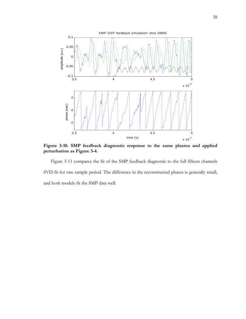
38

3.5 4 4.5 5

x 10-3

-0.1

-0.05

0

0.05

0.1SMP DSP feedback simulation: shot 19805

ampl

itude

(a.

u.)

3.5 4 4.5 5

x 10-3

-2

0

2

phas

e (r

ad.)

t ime (s)

Figure 3-10. SMP feedback diagnostic response to the same plasma and appliedperturbation as Figure 3-4.

Figure 3-11 compares the fit of the SMP feedback diagnostic to the full fifteen channels

SVD fit for one sample period. The difference in the reconstructed phases is generally small,

and both models fit the SMP data well.

39

-3 -2 -1 0 1 2 3-1

-0.8

-0.6

-0.4

-0.2

0

0.2

0.4

0.6

0.8

1x 10

-3

poloidal angle (rad.)

mode diagnostic reconstructions: shot 19387, t=0.0056

SMPsSVD fitSMP feedback

Figure 3-11. SMP samples and amplitude and phase representations from a fifteenchannels SVD fit and the four channels SMP feedback diagnostic.

3.3 X-ray TomographyHBT-EP’s soft X-ray tomography (XRT) diagnostic consists of thirty-two photodiodes

viewing a poloidal cross-section of the plasma from various horizontal, vertical, and diagonal

locations. The photodiodes respond to plasma emissivity fluctuations that correlate in phase

with poloidal magnetic field fluctuations (Xiao 1998), and are therefore potentially useful as

an m = 2 diagnostic. Two methods of combining XRT fluctuation signals to produce

quadrature m = 2 feedback signals at a level of system complexity similar to the magnetic

diagnostics were investigated. The methods attempt to isolate the fluctuations from the

q = 2 surface and suppress the bright core baseline signal and m = 1 oscillations.

40

3.3.1 Surface-Tangential XRT Feedback Diagnostic

The surface-tangential method employs

four XRT photodiodes arranged as shown

in Figure 3-12. Signals from the horizontal

pair and the diagonal pair are summed

separately to produce quadrature feedback

signals. The aim of the surface-tangential

method is to isolate emissivity fluctuations

at the q = 2 surface by avoiding viewing the

plasma core.

Viewing the rational surface tangentially and summing upper and lower views results in

signals that are smoother and more sinusoidal than alternative approaches, but even under

the best conditions the surface-tangential diagnostic is inferior to magnetic diagnostics. Even

at large signal amplitude the ST-XRT cannot produce the evenly propagating arctangent

signal characteristic of the SMP diagnostic and required for successful quadrature feedback

(Figure 3-13).

Figure 3-12. Surface-tangentialphotodiode arrangement.

41

2 2.2 2.4 2.6 2.8 3 3.2 3.4 3.6 3.8 4

x 10-3

-2

-1

0

1

2x 10

-3

ampl

itude

(a.

u.)

Surface-tangential XRT simulation: shot 19387

2 2.2 2.4 2.6 2.8 3 3.2 3.4 3.6 3.8 4

x 10-3

-2

0

2

phas

e (r

ad.)

t ime (s)

Figure 3-13. Surface-tangential XRT diagnostic response to a growing 2/1 mode.

There are probably many

reasons for the unreliability of the

ST-XRT, but the most important

one is that the moving average of

the soft x-ray signal can change at

the same rate or faster than the

fluctuations (Figure 3-14). Fourth-

order DSP 2.5 kHz high-pass filters

were simulated to remove low frequency baseline fluctuations, but baseline excursions in the

fluctuation frequency range pervade the signals and degrade performance.

0 0.001 0.002 0.003 0.004 0.005 0.006 0.007 0.008 0.009 0.010

0.005

0.01

0.015

0.02

0.025

0.03

0.035

0.04

lum

ines

cenc

e (a

.u.)

time (s)

Figure 3-14. Unfiltered soft X-ray signal.

42

3.3.2 Surface-Normal XRT Feedback Diagnostic

The aim of the surface-normal method

is to maximize the amplitude of the m = 2

signal by viewing one plasma diameter and

subtracting a 90º intersecting diameter to

reduce the common plasma core signal and

enhance the signal that varies like cos 2θ

(Figure 3-15). Unfortunately, the plasma

core is so much brighter than the layer

outside the rational surface that the error in

subtraction is often greater than the level of

the m = 2 fluctuations.

2 2.2 2.4 2.6 2.8 3 3.2 3.4 3.6 3.8 4

x 10-3

-2

-1

0

1

2x 10

-3

ampl

itude

(a.

u.)

Surface-normal XRT simulation: shot 19387

2 2.2 2.4 2.6 2.8 3 3.2 3.4 3.6 3.8 4

x 10-3

-2

0

2

phas

e (r

ad.)

t ime (s)

Figure 3-16. Surface-normal XRT diagnostic response to a growing 2/1 mode.

Figure 3-15. Surface-normal photodiodearrangement.

43

We believe both XRT methods have the potential to achieve better elimination of core

contributions and increased m = 2 sensitivity with the addition of more views and more

hardware. However, the SMP diagnostic performed much better with existing hardware, and

development of the XRT feedback diagnostics was discontinued.

3.4 SummaryFour feedback diagnostics were developed using magnetic and optical diagnostics in

HBT-EP. The Rogowski diagnostic had more phase error at low mode amplitudes than the

SMP diagnostic. The Rogowski diagnostic also loses quadrature when control perturbations

are applied, and the SMP diagnostic does not. The shell-mounted probes created the best

feedback signals. A technique for producing quadrature signals from four arbitrarily placed

probes is described and compared to the full fifteen-channel diagnostic. Of the two optical

methods investigated, the one utilizing views tangent to the 2/1 rational surface had the

better performance, but both were inferior to magnetic diagnostics.

44

4 Feedback Control CoilsThe m = 2, n = 1 control coils of HBT-

EP are constructed from nine turns of #1

stranded copper cable, wound on a template

to match the curvature of the vacuum

vessel. A pair of coils are strapped tightly

around the vacuum vessel directly over the

quartz insulator and stainless steel flanges at

the junction between two segments,

forming an m = 2 set (Figure 4-1). For the

feedback experiments described in this

thesis, a pair of saddle coil sets is driven

with the cosine phase of the perturbation

signal, and another pair of sets is driven

with the sine phase. The saddle coils are oriented so that the cosine and sine sets

approximate two helical windings, separated by 90º in toroidal (or electrical) angle.

The saddle coils induce eddy currents in the stainless steel flanges directly underneath

which, by Lenz’s law, tend to cancel the toroidal flux and reduce the m = 0 component of

the applied perturbation from the poloidal segments of the saddle coils. Locating the

toroidal segments of the saddle coils directly outside the quartz insulating rings allows fast

penetration of the applied fields.

Figure 4-1. Top half of m = 2 saddle coilmounted over quartz insulator ring andvacuum vessel flanges.

45

4.1 Saddle-Flange ModelThe saddle coil set and flanges are modeled in cylindrical geometry to determine the

flange currents that optimally cancel the toroidal flux. Each flange opposes the flux due to

the saddle coils and the opposite flange. The solution turns out to be approximately ±1.6 A

for each ampere in the nine-turn coils. The arrows in Figure 4-2 and Figure 4-3 show

zaBB ˆ⋅− inside the flange; the surface color scale refers to the value of Bz. Figure 4-3 shows

the cancellation of the m = 0 component of B by the flange eddy currents.

Figure 4-2. Saddle coil set and stainless steel flange model with zero flange current.

46

Figure 4-3. Saddle coil set and stainless steel flange model with Iflange/Isaddle = 1.6

The flange current to saddle current ratio is used to model the effect of the two phase

saddle coil set and flanges on the q = 2 surface, represented by a toroidal surface current.

The helical surface current function is

( )( )

+

+⋅Φ++=

20

2

00

4

ˆ2ˆ2cos

Rr

RrtK

s

s φθφθaa

K (4.1)

Its magnitude is determined by solving dSRS∫×=

30

4RK

Bπµ

for K0. For typical HBT-EP

parameters ( ( )aB~ = 5×10-4 T, rs = 0.09 m) K0 ≈ 4 kA/m.

The model of the toroidal q = 2 surface and saddle-flange sets is used to quantify the

K××B forces and torques on the rational surface and the Fourier mode spectrum of Br. The

magnetic field is determined by totaling ∫×=3

0

4 R

dNI RLB

πµ

of all saddle coils and flanges

on a uniformly spaced grid representing the rational surface (Figure 4-4). Eddy currents

47

induced in the vacuum vessel and conducting shells are neglected. The mode spectrum is

calculated from a two-dimensional FFT of the Br grid.

Figure 4-4. B r on q = 2 surface. Cosine and sine coil sets carry equal current.

4.2 Saddle Perturbation Mode SpectrumAnalysis of the mode spectrum of Br reveals that just two modes with 2=nm

contribute a significant fraction of the total field: m/n = 2/±1. The field fraction is defined

here as ( ) PPP mn−−1 , where P is the total power in all modes, and Pmn is the power in

mode m, n. Figure 4-5 shows little excitation of adjacent n = ±1 modes at the q = 2 surface.

48

1 2 3 4 50

0.5

1

1.5

2

2.5

3

3.5

4

4.5

m

n = +1n = -1

Figure 4-5. Field fractions at the q = 2 surface of the first five n = ±1 modes by thecosine coil set. Sine coil set fractions are similar, except B(2,-1) ~ 3.4%, due todifferences in orientation and toroidal spacing.

Due to the short toroidal extent of each saddle coil, the m = 2 spectrum is spread out in

n (Figure 4-6). The 2/1 mode represents approximately 4% of the total field. This fraction is

useful in scaling experimental saddle currents to the helical current sheets often encountered

in tearing mode theory.

49

-30 -20 -10 0 10 20 300

1

2

3

4

n

Figure 4-6. Field fraction of m = 2 components from cosine coil set. The 2/1 mode ishighlighted. The spectrum of the sine coil set is similar, with ~4% 2/1 componentand slightly different 2/n mode amplitudes.

The 4% field fraction for the 2/1 coil set determined above is an order of magnitude

smaller than the value expected from a crude estimate based on coil coverage area. One

phase of the nine-turn saddle coil set covers ~3.5% of the area of the torus, which has an

equivalent surface-area average field of ~30% of a single-turn full helical winding.

4.3 Forces and Torques at the Rational SurfaceThe radial and poloidal forces on the mode are in quadrature and vary with the phase

difference between the mode and the applied perturbation. The zero phase is defined here as

the phase when the mode toroidal current is aligned with the like toroidal saddle currents in

the cosine coil set. At the zero phase the outward radial force on the mode is at a maximum

(Figure 4-7).

50

Figure 4-7. K××B forces on a helical current sheet at the zero phase, with equal currentin cosine and sine saddle coil sets.

For a 4 kA/m current sheet, the maximum of the radial and poloidal forces is ~1×10-3

newtons per ampere of saddle current. The toroidal force is an order of magnitude smaller,

but because of HBT-EP’s low aspect ratio the toroidal and poloidal torques are comparable

(Figure 4-8). Strong damping of the poloidal rotation (Stix 1973) implies that mode rotation

is solely dependent on the toroidal torque. In this current sheet model the maximum toroidal

torque phase is shifted away from the expected value of +90º. A possible explanation for

this is that eddy currents flowing around the stainless steel flanges’ circumference create local

m = 0 radial magnetic fields that shift the phase of maximum toroidal torque. It is difficult to

observe this phase shift experimentally with HBT-EP’s present diagnostic set. If the phase

shift is present it would reduce the effectiveness of negative feedback and of open loop

attempts to increase mode amplitudes because the maximum toroidal torque phase is shifted

and the maximum radial force phase is not.

51

0 30 60 90 120 150 180 210 240 270 300 330 360

-1

-0.5

0

0.5

1

1.5x 10

-4

feedback phase (deg)

torq

ue p

er a

mpe

re (

N-m

/A)

poloidaltoroidal

Figure 4-8. Poloidal and toroidal torques (per ampere of saddle current) on a 4 kA/mhelical current sheet. Current is flowing only in the cosine coil set.

4.4 Feedback Model ConventionsThe conventions used in this model will be applied to analysis of the experimental results

in the next two chapters. The toroidal coordinate system is right handed. Positive poloidal

angle (θ) points up on the outboard side of the torus. Positive toroidal angle (φ) points

clockwise on a top view of the torus. The 2/1 mode propagates in the positive direction in

these two coordinates.

Table 4-1 displays the convention for

the feedback phase angle, defined as

modesaddle Φ−Φ≡∆Φ . The physical phase

differences between the mode diagnostic

signals and the saddle coil signal are measured using a method described by Morris et al.

(1990) of amplifying the saddle coil pickup of MHD activity during a plasma discharge (shot

16145) and cross-correlating with the mode diagnostic signal. By Lenz’s law this saddle coil

pickup is in the negative feedback phase and, preserving the convention,

Table 4-1. Feedback phase convention.

0º Positive feedback ( 0>W& ).90º Positive (advancing) torque ( 0>ω& ).180º Negative feedback ( 0<W& ).270º Negative (retarding) torque ( 0<ω& ).

52

.. physdiagmode Φ−+Φ=Φ π . The physical angle Φphys is m times the physical toroidal

separation between the saddle coil set zero and the mode diagnostic zero (56°). The

quadrature m = 2 fit of the fifteen SMP signals is adjusted by adding 26º to the diagnostic

phase, and the m = 2 Rogowski signal is adjusted by adding 71º to the diagnostic phase

(Figure 4-9).

Figure 4-9. Cross-correlation of saddle-coil MHD pickup and mode diagnostics.Plots show correlation absolute value (normalized) vs. correlation phase in the band5–25 kHz.

4.5 SummaryThe magnetic field perturbation generated at the surface of a toroidal 2/1 current sheet

by a two-phase set of two-quadrant saddle coils is modeled. The effects of ideal eddy

currents flowing in adjacent circular flanges are included and are shown to reduce the

unwanted local m = 0 components from the two-quadrant coil. The flange eddy currents

may alter the quadrature relationship between radial force and toroidal torque on the current

sheet, but this effect was not observed experimentally. Approximately 4% of the total

53

perturbation is resonant with the 2/1 mode, providing a useful fraction for scaling the saddle

current to an equivalent helical current. The conventions for the model and for analysis of

feedback experiments are defined in a right-handed toroidal coordinate system.

54

5 Phase Instability MeasurementsThe phase instability determines the bandwidth of a feedback system by requiring it to

respond to feedback phase changes faster than the phase instability growth rate to maintain

negative feedback. In this chapter the phase instability growth rate is measured by observing

the response of a saturated 2/1 tearing mode to a resonant magnetic perturbation in the

negative feedback phase. Theoretical predictions of the growth rate are calculated using

measured HBT-EP discharge parameters. The predictions are shown to be in good

agreement with the experimental measurements of the phase instability growth.

The amplitude of the mode is expected to decrease while the RMP is in the negative

feedback phase, but it is observed that the rate of decrease is greater than the rate predicted

by balancing Rutherford island growth against opposing Lorentz forces induced by the

saddle coils. As indicated in Section 2.4, an additional term dependent on the mode’s

deviation from its natural frequency can explain this enhanced attenuation.

5.1 Experimental TechniqueThe phase instability is observed in HBT-EP by applying a rotating RMP until the

magnetic island locks to the perturbation and rotates synchronously with it. The phase of the

perturbation is then rapidly advanced 180º in what is referred to as a “phase flip.” The

dynamics of the phase instability can be studied while the mode is re-locking to the RMP.

The phase instability time scale is estimated by noting the initial phase difference prior to

the phase flip, and measuring the elapsed re-locking time after the flip until the phase

difference returns to its initial value.

55

5.2 ObservationsExperimental signals from a phase flip discharge are shown in Figure 5-1. After the

phase flip, the mode initially slows and attenuates, then accelerates back to the perturbation

frequency and recovers most of its initial amplitude as it re-locks to the RMP. After the

phase flip, the mode is in the retarding torque phase and the mode frequency reduces

rapidly. The mode phase overshoots the RMP slightly before re-locking in the positive

feedback phase. The 2/1 frequency is not always reduced following a phase flip; it will

increase when the post-flip phase is associated with advancing torque.

Figure 5-1. Saddle coil currents, m = 2 signals, and phase difference signal of a phaseflip discharge. The perturbation phase flip (-180°°) occurs just before 4.3 ms. Themode slows to re-lock with the regressed perturbation. The re-locking period iswithin the shaded area.

56

5.2.1 Mode Suppression from Ion-Inertial Effects

The reduction in mode amplitude following a phase-flip cannot be explained solely by

the action of the applied perturbation in the negative feedback phase. Figure 5-1 shows the

mode suppression persisting after the mode has returned to the positive feedback phase. The

extra suppression accompanies shifts in mode frequency away from the natural frequency.

The dynamics of the phase instability are simulated using the normalized model of

Section 2.6. Figure 5-2 shows the evolution of b, ∆Φ, and Ω, during a phase flip discharge.

The inertial damping of the 2/1 mode amplitude is caused by the large frequency drop after

the phase-flip. The inertial damping is transient; after the mode re-locks to the perturbation

it regains the perturbed growth rate. Neglecting the inertial damping term in simulation (by

setting g3 = 0) yields results which deviate from observed mode amplitude behavior, while

retaining good agreement with observed frequency and phase evolution.

Figure 5-2. Simulation of 2/1 mode response to a phase-flip discharge andcomparison to experiment. The phase flip occurs at 0.5 ms. Simulation g 3 = 8,000.The trace with g 3 = 0 shows the result of neglecting the effect of frequency-dependent inertial damping on mode amplitude.

57

5.3 Phase-Flip TimescaleThe phase flip timescale τ2/1 can be estimated by neglecting viscosity, assuming a

constant-frequency perturbation at ω0, and rewriting the island rotation equation (2.13) as

( ) 21/2sin τ∆Φ=Φ∆ && . The normalized model gives ( ) 2/1

021/2

−= AIbh ωτ . A different

formulation of island rotation (Lazzaro and Nave 1988), which treats the island moment of

inertia as independent of island width, has a better form for using measurable plasma

parameters to estimate the phase instability timescale. In HBT-EP the mode amplitude does

not span a wide enough range to distinguish one model from the other. The simpler form is

bA

srBI

rRθ

ρτ ~2 0

01/2 ≈ (5.1)

where rb is the radius of a helical control coil carrying current IA. The 2/1 surface has minor

radius rs and major radius R0. The fluctuating magnetic field outside the rational surface is

proportional to ( )1+− mr , so the measured ( )rBθ~ of the 2/1 mode is scaled by ( ) 8.43 ≈ssmp rr

to give the value at the rational surface. The helical control current IA is estimated by

multiplying the measured saddle coil current by 4%, the 2/1 fraction of the perturbation

determined in Section 4.2.

5.4 ResultsTable 5-1 lists the measured model quantities averaged over a 500 µs period prior to the

phase flip, the calculated theoretical phase instability time scale (τ2/1), and the measured re-

locking time (tlock) for twelve discharges. The applied perturbation current spans a 4× range,

and the mode amplitude spans a 6× range, producing time scales and re-locking times

ranging approximately from 100–300 µs. Agreement is good within the examined range.

58

Table 5-1. Phase instability measured model quantities and experimental results.

Shot R0

(cm)ñ0

(10-8 kg/m3)IA

(A) θB~

(mT) τ2/1

(µs)tlock

(µs)% diff.

12976 93.5 2.01 24.2 4.7 89.5 120 -25%13479 93.2 2.17 20.6 5.3 301 317 -5%16451 94.3 2.12 10.0 2.7 191 215 -11%16453 93.7 2.11 5.5 1.6 336 334 1%18986 95.2 2.12 13.2 2.9 163 169 -4%19493 94.1 0.92 12.4 0.8 213 218 -2%19496 93.5 0.88 13.5 1.8 129 118 9%19499 93.8 0.90 13.4 2.0 125 152 -18%19513 93.6 0.88 13.3 2.1 120 184 -35%19514 94.1 0.93 13.3 1.9 132 160 -18%19516 93.9 0.90 13.1 2.1 122 124 -2%19519 94.0 0.91 12.0 2.2 125 90 39%

The predicted time scales and measured re-locking times are plotted in Figure 5-3.

Figure 5-3. Measured phase instability re-locking times vs. predicted time scales.

59

5.5 SummaryAn open-loop procedure for producing and measuring the phase instability with natural

tearing modes is presented. Simulations of mode dynamics during phase-flip discharges

show the importance of a frequency-dependent stabilizing term to explain mode amplitude

behavior. Measured quantities are used to predict the phase instability time scale for selected

discharges and the measured re-locking periods are found to be in good agreement with the

predicted time scales.

60

6 Feedback ExperimentsHBT-EP’s 2/1 feedback loop consists of a mode diagnostic, a digital signal processor,

high-power amplifiers, saddle-shaped control coils, and a collection of analog interface and

isolation electronics. The quadrature mode diagnostics are described in Chapter 3, the saddle

coils in Chapter 4. The DSP hardware, amplifiers, and interface electronics are covered in

Appendix A. In this chapter the feedback loop is analyzed in time and frequency domains to

illustrate how DSP latency affects the loop performance. Observations of feedback on

saturated and unsaturated modes are presented, and the effect of the phase instability on

feedback phase accuracy is quantified.

6.1 The Feedback AlgorithmThe algorithm used in the 2/1 feedback experiments is a vector phase-rotation matrix. It

utilizes the quadrature input poloidal field fluctuations to produce quadrature output control

currents rotated by δ and amplified by G.

ΦΦ

⋅

−⋅=

ΦΦ

−

−

1

1

sin~

cos~

cossin

sincos

sin

cos

n

n

n

n

B

BG

I

I

θ

θ

δδδδ

(6.1)

The implementation of (6.1) in DSP machine language using the four-channel SMP feedback

diagnostic is given in Section A.2.

6.2 Feedback SimulationThe normalized 2/1 model is used to simulate mode evolution over a 1 ms period with

an initially saturated (b = 1) mode rotating at the natural frequency (Ω = 1). Constant

feedback is simulated by holding the phase difference (∆Φ) fixed and varying the applied

control current with a gain proportional to b. Figure 6-1 plots the values of b and Ω after

61

1 ms of constant feedback for different feedback phases. Inertial damping due to increases

and decreases in Ω causes the reduction in b; reduction at perfect negative feedback (180º) is

close to zero.

Figure 6-1. Simulated 2/1 mode amplitude and frequency modification under idealfeedback vs. constant feedback phase. The mode is initially at b = 1, ΩΩ = 1 at T = 0.G = 5.

6.2.1 Latency Effects

The ideal feedback system simulated above has zero latency; it responds instantaneously

to a change in the input state. The real DSP feedback system has a finite clock frequency,

and can change its output state only every 10 µs. Latency effects are simulated by holding

the simulated perturbation phase and amplitude fixed over each sampling period, while the

mode equations are integrated with a Runge-Kutta method on a finer time increment. Phase

and amplitude errors accumulate between samples and reduce feedback effectiveness. The

values of b and Ω after 1 ms of feedback with nonzero latency are plotted in Figure 6-2. The

62

clockwise rotation of the curves from the ideal case is a product of the latency. The value of

∆Φ at T = 1 ms is shifted from the programmed ∆Φ.

Figure 6-2. Simulated normalized amplitude and frequency values after feedbackwith 10 µµs latency, over a 1 ms period. The simulation demonstrates reduced controlover the feedback phase difference. G = 5.

6.3 Frequency-Domain AnalysisThe feedback loop and algorithm are analyzed in the s-domain by using a phasor

representation of the island magnetic fluctuations ( tiBeB ω= ) as input to the feedback loop

transfer function. Because the digital algorithm contains no internal delays, the system may

be analyzed without employing discrete z-transforms. The DSP latency is modeled by a time

delay ( DsTe− ). Control signals proportional to the phase difference between the saddle

currents and the mode are calculated by taking the time product of the feedback current

phasor with the conjugate of the mode phasor. This involves a convolution integral in the

frequency domain

63

( ) ( ) ( ) ( ) ( ) ( )dppsBpIi

sBsItBtIeIBC

i −=∗⇒⋅= ∗∗∗∆Φ ∫π21

(6.2)

A block diagram of the feedback loop is shown in Figure 6-3. The shell probe signals are

modeled by shifting the mode phasor by the proper angle to represent the probe poloidal

positions, and taking the real part. Input and output coupling transfer functions are

simplified to exclude the poles of higher-bandwidth components like the DSP isolation

network. High bandwidth equipment is treated like a static gain. The DSP implementation of

the SMP diagnostic and feedback algorithm are performed in continuous time, with the

aforementioned delay representing the DSP latency. The output quadrature currents are

converted to a phasor and used to create frequency-domain functions of the feedback

control parameters ∆Φ= cosII D , ∆Φ= sinIIQ .

( )sB

shell probes RC integration DSP input coupling

−

−

−

−

1

2

3

4

2

2

2

2

Re

ϕ

ϕ

ϕ

ϕ

i

i

i

i

e

e

e

e

sNA11

1

+τsG

12

22

+ττ

s

Gs

−

−0101

1010

Common modesubtraction

2221

1211

qq

qq

quadraturecorrection

−δδδδ

cossin

sincos3G

feedback gain & phase shift

DsTe−

DSP latency

24

4

+τsG

output coupling

[ ]iG 15

saddle current

( )sI( )B

sBsI ∗∗)(

s-convolution

QD iII +

tearing mode model

( )( )IBh

IBg

,

, B&

ω&

Figure 6-3. Block diagram of the feedback loop transfer function. Frequencyconvolution of the output current and input field allow s-domain analysis of thefeedback-produced force and torque.

The ideal feedback loop in Figure 6-3 takes a simpler form through symmetry in the

transfer functions of the multiple input and output channels. The output saddle current

phasor can be represented by ( ) ( ) ( ) δiesBsHsI −= , where

( ) ( )( )( )112 124

2

+++=

−∏

τττ sss

esGsH

DsT

(6.3)

64

The s-domain function for the feedback-phase dependent currents with phasor input

( ) ( )ωisBsB −= is given by

( ) ( ) ( ) ( )[ ]∑ −=+≡ ∗−Π

kkkk

iQD psBpBpHe

B

GiIIsI Resδ (6.4)

with the residues evaluated at each pole pk of the bracketed expression.

Figure 6-4 plots the frequency response of I at a single value of feedback δ. For a mode

initially at 10 kHz, the forces (at this δ) tend to increase mode frequency to approximately

20 kHz. Rapid doubling of the mode frequency under feedback is observed regularly in

HBT-EP. At 20 kHz, the mode attenuating portion of the perturbation is cut to a third of its

initial value.

0 0.5 1 1.5 2 2.5

x 104

-800

-600

-400

-200

0

a.u.

)

Feedback loop frequency response

0 0.5 1 1.5 2 2.5

x 104

0

200

400

600

a.u.

)

system frequency (Hz)

Figure 6-4. Frequency response of DSP feedback loop (δδ = 0). As system frequencyincreases, mode attenuating force (ID) decreases, and mode accelerating torque (IQ)increases.

A contour map of the frequency response of ID over the range of feedback δ is shown in

Figure 6-5. The frequency-dependent shift of the contours is produced primarily by the loop

65

latency (10 µs). Although ID varies little over the range ω > ω0 when operating at δ ~ -90º,

IQ is strongly decelerating at that δ.

0.5 1 1.5 2 2.5

x 104

-180

-90

0

90

180

system frequency (Hz)

deg.

)direct feedback current ID frequency response (% of DC maximum)

-90

-90

-90

-90

-70.7

-70.7

-70.7

-70.7-70.7 -70.7

-50

-50

-50

-50

-50

-33

-33

-33

-33

-33

0

0

0

0

0

0 33

33

33

33

50

50

50 50

70.7

70.7 70.7

90 90

90

Figure 6-5. Map of direct feedback current magnitude vs. frequency and feedback δδ.

6.4 Observations

6.4.1 Unsaturated Modes

Figure 6-6 shows the m = 2 evolution and feedback response signal for an HBT-EP

discharge with an initially small, unsaturated mode. The saddle currents follow but do not

suppress mode growth. Mode frequency is doubled or halved in 100 µs just before 6 ms.

Such rapid changes in mode frequency increase feedback latency error by the larger and

more unpredictable component ∫T

dt0ω& in addition to the relatively constant T0ω for an

evenly rotating mode.

66

A/T

Figure 6-6. Tearing mode DSP feedback signals for an unsaturated mode. Feedbackis applied between 4.5 and 6.5 ms.

6.4.2 Saturated Modes

Feedback quadrature signals with a saturated mode are shown in Figure 6-7. Increases in

mode frequency correlate with ∆Φ shifts away from 180° towards the advancing torque

phase, and increasing mode amplitude. This relationship between the feedback signals

demonstrates direct attenuation of the mode. Mode attenuation is modest as expected with

the HBT-EP plasma and coil geometry.

67

A/T

Figure 6-7 Tearing mode DSP feedback signals for a saturated mode. Feedback isapplied between 5 and 7 ms.

6.4.3 Phase Instability and Feedback

The phase instability affects feedback by increasing the magnitude of phase and

frequency deviations as feedback gain increases. The feedback loop becomes less able to

maintain phase accuracy as gain increases. This effect was investigated by producing closed-

loop feedback discharges at a constant δ , but at different levels of gain. Mode amplitude was

nearly constant in these discharges. From (5.1), the phase instability time scale should be

inversely proportional to G1/2. The effect is quantified by measuring the deviation of the

average achieved feedback phase difference from the expected phase difference programmed

by selecting δ. The average mode frequency increases linearly with G1/2 and increases the

loop phase error due to DSP latency. The deviation of feedback phase is plotted against G1/2

in Figure 6-8.

68

Figure 6-8. Variation of the feedback phase difference (∆∆ΦΦ) and deviation of its mean

from the programmed feedback phase difference (δδ), vs. G . In this plotG ≡≡ <IA/B>.

6.5 SummaryFrequency-domain analysis of the feedback loop predicts a significant decrease in

available direct feedback current as mode frequency approaches 2ω0, due to DSP latency.

The feedback loop follows but does not prevent 2/1 growth. Modest attenuation is observed

with saturated modes as expected for the HBT-EP plasma and coil geometry. With rB~

nearly constant and I increasing with feedback gain, the phase deviation increases with gain

to further limit phase control. We believe this effect is a result of the phase instability.

69

7 Conclusion

7.1 Summary of ResultsFour mode detection diagnostic techniques were compared. We observe a loss of

quadrature in the m = 2 Rogowski coil mode diagnostic during feedback discharges. Two

optical mode detection techniques, at a similar level of system complexity to the magnetic

techniques, were investigated and yielded poor results. A diagnostic based on four Mirnov

probes mounted on a conducting shell 1 cm from the plasma edge was the most reliable of

the four techniques.

Numerical calculation of the magnetic fields produced by the two-phase 2/1 saddle coil

set show that approximately 4% of the total field produced is resonant with the 2/1 mode at

the rational surface. The field spectrum is spread out in toroidal mode number n due to the

small toroidal extent of the saddle coils. Calculated field fractions indicate very little

excitation of other n = 1 modes with this coil set.

Experimental observations of the phase instability time scale show excellent agreement

with theoretical predictions over a 6× range of mode amplitudes. Reduction in mode

amplitude following the phase flip continues past the mode’s re-locking to the positive

feedback phase. This continued amplitude reduction is modeled well by considering ion-

inertial damping due to frequency shifts away from the natural mode rotation frequency.

The HBT-EP 2/1 feedback system follows but cannot prevent the growth of

unsaturated modes. It can slowly reduce the amplitude of saturated modes. Amplifier

current, DSP latency, and coil geometry limit available loop gain. The 2/1 mode frequency is

observed to fluctuate more rapidly than the DSP feedback controller can follow. The phase

instability limits feedback performance by increasing the magnitude of these fluctuations

70

away from negative feedback, and therefore the fraction of time spent outside of the

negative feedback phase range, as feedback gain increases.

7.2 Discussion of ResultsThe feedback experiments in HBT-EP point out the importance of the phase instability

as a factor limiting feedback performance and the necessity of a frequency-dependent

stabilizing term to explain mode behavior. The phase instability time scale grows longer in

larger, denser tokamaks. ITER’s τ2/1 could be 1.5 ms.

Maximum amplifier current, the phase instability, and DSP latency all contribute to

reducing feedback mode attenuation, but coil geometry plays a large role. Saturated mode

attenuation can be dramatically increased, with the phase instability time scale also modestly

increased, by reducing the coil radius. An ITER feedback system with rb/rs = 1.2 and

Wsat/rs = 5% has a control current requirement close to that for HBT-EP, despite a 1,000×

difference in plasma current. Increasing coil toroidal coverage would also be helpful, but

improvements in mode attenuation are assumed to be linear with increasing coil coverage

area, but vary with the inverse square of coil radius.

7.3 Suggestions for Future WorkThe knowledge gained from analysis of the feedback system in this thesis should be

useful for designing the next system. DSP latency should be minimized by increasing the

sampling rate. Adding differential feedback could help the loop track fast changes in mode

frequency due to the phase instability.

The 2/1 tearing mode model described in Chapter 2 does a good job of simulating mode

rotation, but its accuracy in simulating mode amplitude behavior has room for improvement.

Future experiments should explore the frequency-dependent stabilization of island width

and address the issue of island moment of inertia.

71

Numerical models can be extended to determine the efficacy of a set of saddle coils as a

function of toroidal localization and radius. The shift in maximum toroidal torque phase in

the modeled saddle coil set might be observed experimentally with different diagnostic

techniques.

72

8 References

Cited ReferencesAnalog Devices, Inc. 1995. ADSP-21000 Family Applications Handbook. Vol. 1.

Arsenin, V. V. et al. 1978. Feedback stabilization of kink instability in the TO-1 tokamak. InProceedings of the Seventh International Conference on Plasma Physics and Controlled Nuclear FusionResearch. Vol 1. Vienna: International Atomic Energy Agency. 233–45.

Bernstein, I. B. et al. 1958. An energy principle for hydromagnetic stability problems.Proceedings of the Royal Society of London A 244: 17–40.

Bol, K. et al. 1975. Experiments on the Adiabatic Toroidal Compressor. In Proceedings of theFifth International Conference on Plasma Physics and Controlled Nuclear Fusion Research. Vol. 1.Vienna: International Atomic Energy Agency. 83–97.

Burr-Brown Corporation. 1994. Integrated Circuits Data Book, Linear Products.

Cerf, Christopher and Victor Navasky. 1998. The Experts Speak. Rev. ed. New York: Villard.

Edery, D., et al. 1983. Inertial and viscous effects in the nonlinear growth of the tearingmode. Physics of Fluids 26 (5): 1165–7.

Fitzpatrick, R. and T. C. Hender. 1991. The interaction of resonant magnetic perturbationswith rotating plasmas. Physics of Fluids B 3 (3): 644–72.

Fitzpatrick, R. 1993. Interaction of tearing modes with external structures in cylindricalgeometry. Nuclear Fusion 33 (7): 1049–1084.

Furth, H. P., J. Killeen, and M. N. Rosenbluth. 1963. Finite-resistivity instabilities of a sheetpinch. Physics of Fluids 6 (4): 459–84.

Furth, H. P., P. H. Rutherford, and H. Selberg. 1973. Tearing mode in the cylindricaltokamak. Physics of Fluids 16 (7): 1054–1063.

Gates, D. 1993. Passive stabilization of MHD instabilities at high βn in the HBT-EPtokamak. Ph.D. dissertation, Columbia University, New York.

Gibson, A. and the JET Team. 1998. Deuterium-tritium plasmas in the Joint EuropeanTorus (JET). Physics of Plasmas 5 (5): 1839–47.

Gross, Robert A. 1984. Fusion Energy. New York: John Wiley & Sons.

73

Hegna, C. C. 1998. The physics of neoclassical magnetohydrodynamic tearing modes. Physicsof Plasmas 5 (5): 1767–74.

Ivers, T. H. et al. 1996. Observation of wall stabilization and active control of low-nmagnetohydrodynamic instabilities in a tokamak. Physics of Plasmas 3 (5): 1926–34.

Lanouette, William, with Bela Silard. 1992. Genius in the Shadows. New York: CharlesScribner’s Sons.

Lazzaro, E., and M. F. F. Nave. 1988. Feedback control of rotating resistive modes. Physics ofFluids 31 (6): 1623–9.

Monticello, D. A., R. B. White, and M. N. Rosenbluth. 1978. Feedback stabilization ofmagnetic islands in tokamaks. In Proceedings of the Seventh International Conference on PlasmaPhysics and Controlled Nuclear Fusion Research. Vol. I. Vienna: International Atomic EnergyAgency: 605–14.

Monticello, D. A. and R. B. White. 1980. Nonlinear drift tearing modes. Physics of Fluids 23(2): 366–71.

Morris, A. W. et al. 1989. Feedback stabilization of disruption precursor oscillations. InProceedings of the Sixteenth European Conference on Controlled Fusion and Plasma Physics. Vol. 2.Switzerland: European Physical Society. 541–44.

Morris, A. W. et al. 1990. Feedback stabilization of disruption precursors in a tokamak.Physical Review Letters 64 (11): 1254–57.

Nave, M. F. F. and J. A. Wesson. 1990. Mode locking in tokamaks. Nuclear Fusion 30 (12):2575–83.

Navratil, G. A. et al. 1988. Active control of 2/1 magnetic islands in a tokamak. Physics ofPlasmas 5 (5): 1855–63.

Reass, W. A. et al. 1987. Design, construction, and electrical test results of a 4 channel, 52megawatt equilibrium amplifier system for ZT-P. (submitted at IEEE meeting, Monterey,California).

Rutherford, P. H. 1973. Nonlinear growth of the tearing mode. Physics of Fluids 16 (11):1903–8.

Smolyakov, A. I. et al. 1995. Rotating nonlinear magnetic islands in a tokamak plasma. Physicsof Plasmas 2 (5): 1581–98.

Stix, T. H. 1973. Decay of poloidal rotation in a tokamak plasma. Physics of Fluids 16 (8):1260–7.

Sykes, A. and J. A. Wesson. 1980. Major disruptions in tokamaks. Physical Review Letters 44(18): 1215–18.

74

Vijaya Sankar, M. K. et al. 1993. Initial high beta operation of the HBT-EP tokamak. Journalof Fusion Energy 12 (3): 303–310.

Waddell, B. V. et al. 1978. Mechanism for major disruptions in tokamaks. Physical ReviewLetters 41 (20): 1386–9.

White, R. B. 1986. Resistive reconnection. Reviews of Modern Physics 58 (1): 183–207.

Wilson, David. 1983. Rutherford. London: Hodder and Stoughton.

Wilson, H.R. et al. 1996. Threshold for neoclassical magnetic islands in a low collisionfrequency tokamak. Physics of Plasmas 3 (1): 248–65.

Xiao, Q. 1998. Effect of applied resonant magnetic perturbations on the measured MHDmode structure in a tokamak plasma. Ph.D. dissertation, Columbia University, New York.

General ReferencesBanks, Stephen P. 1986. Control Systems Engineering. London: Prentice-Hall International.

Freidberg, Jeffrey P. 1987. Ideal Magnetohydrodynamics. New York: Plenum Press.

Hayt, William H., Jr. 1989. Engineering Electromagnetics. 5th ed. New York: McGraw-Hill.

Jackson, John David. 1975. Classical Electrodynamics. 2d ed. New York: John Wiley & Sons.

Wesson, John. 1987. Tokamaks. The Oxford Engineering Science Series, no. 20. New York:Oxford University Press.

75

A DSP Hardware And SoftwareHBT-EP requires a collection of hardware, software, and interfacing equipment to

perform feedback experiments. The DSP hardware is controlled and programmed via a host

computer. The DSP analog interface is electrically isolated from the tokamak by a network

of optical isolation amplifiers. The saddle coils are powered by two high-power amplifiers.

These components of the feedback loop are described below.

A.1 DSP HardwareThe DSP hardware is manufactured by Bittware, Inc. The Snaggletooth-PCI DSP card

connects to the PCI bus of the host computer and contains two Analog Devices ADSP-

21062 Super Harvard Architecture (SHARC) processors. Harvard architecture computers

have separate data and program memory and can read one instruction, perform another, and

read or write a data word, all in the one clock cycle. The processors used in HBT-EP operate

on a 40 MHz clock with 32-bit memory and I/O busses. The Bitsi-DAQ I/O mezzanine

mounts on the DSP card, and provides eight channels of simultaneous 12-bit A/D

conversion at 500 kHz and four channels of 14-bit D/A conversion at 100 kHz.

A.2 SMP Feedback AlgorithmThe SMP feedback algorithm (6.1) is implemented in ADSP-21062 assembly language.

The two DSP processors are configured as master and slave. The master processor

implements the SMP feedback diagnostic and the slave processor performs the feedback

rotation and amplification.

A.2.1 Master Processor Code

The master processor code samples the four shell-mounted probe signals, converts the

samples to floating-point voltages, and produces quadrature signals by correcting for the

76

arbitrary locations of the probes, according to (3.4). The quadrature feedback signals are

placed in message registers and the slave processor is interrupted to indicate new data. This

code is interrupt driven off of the 2 µs A/D conversion clock.

// code for processor 1 (master)

.PRECISION=32;

#include <def21060.h>

// to ensure valid writes to the 82C54, address and data must be valid for// tAW - tSW + tDW + tWD = 0 - 0 + 140 + 25 ns = 165 ns = 7 cycles.// This macro does 15 NOP's#define timer_delay \

NOP; NOP; NOP; NOP; NOP; \NOP; NOP; NOP; NOP; NOP; \NOP; NOP; NOP; NOP; NOP; \NOP; NOP; NOP; NOP; NOP; \NOP; NOP; NOP; NOP; NOP

#define SHARCB 0x00100000#define VIRPT_VEC 0x00020014

// adc2volts macro takes R0 as adc sample and places floating point volts in F0// clobbers: R0, R1, R2, I0, M0;#define adc2volts \

I0 = a2v_data; \M0 = 1; \R1 = DM(I0, M0); \R0 = R0 XOR R1; \R0 = LSHIFT R0 BY -20; F1 = DM(I0, M0); \F0 = FLOAT R0; \F0 = F0 * F1; F2 = DM(I0, M0); \F0 = F0 - F2

.SEGMENT/DM bitsi;

.PORT bitsidaq[0x10];

.ENDSEG;

.SEGMENT/DM seg_dmda;

.VAR a2v_data[3] = 0x80000000, 2.442002442e-3, 5.0;

.VAR inv_matrix[4] = 0.4808, 0.4808, -0.2955, 0.2955;

.VAR vec[2];

.GLOBAL vec;

.VAR atest = 0;

.GLOBAL atest;

.ENDSEG;

.SEGMENT/PM seg_pmda;

.VAR smp[4];

.ENDSEG;

.SEGMENT/PM seg_rth;

// reserved 0x00NOP; NOP; NOP; NOP;

// reset vector 0x04

77

NOP;JUMP inita;RTI; RTI;

// reserved 0x08NOP; NOP; NOP; NOP;

// stack overflow 0x0CRTI; RTI; RTI; RTI;

// timer=0 0x10RTI; RTI; RTI; RTI;

// vector interrupt 0x14RTI; RTI; RTI; RTI;

// IRQ2 asserted 0x18JUMP irq2a;RTI; RTI; RTI;

.ENDSEG;

.SEGMENT/PM seg_code;

// initialization://

inita:// set proper wait states 1 WSR0 = 0x00529825;DM(WAIT) = R0;

R0 = 0x03000000; // ADC/DAC control wordDM(bitsidaq + 8) = R0; // write ADC/DAC ctrl registerR0 = 0x36000000; // counter 0, timer mode 3DM(bitsidaq + 7) = R0; // write 82C54 controltimer_delay;R0 = 0x14000000; // divide by 20 (500 kHz)DM(bitsidaq + 4) = R0; // write timer 0 counter LSBtimer_delay;R0 = 0x00000000; // MSB = 0DM(bitsidaq + 4) = R0; // write timer 0 counter MSBtimer_delay;R0 = 0xB6000000; // counter 2, timer mode 3DM(bitsidaq + 7) = R0; // write 82C54 controltimer_delay;R0 = 0x05000000; // divide by 5 (100 kHz)DM(bitsidaq + 6) = R0; // write timer 2 counter LSBtimer_delay;R0 = 0x00000000; // MSB = 0DM(bitsidaq + 6) = R0; // write timer 2 counter MSBtimer_delay;BIT SET MODE2 IRQ2E; // make IRQ2 edge-sensitiveBIT SET IMASK IRQ2I; // unmask IRQ2BIT SET MODE1 IRPTEN; // enable interruptsBIT CLR MODE1 CSEL;

ilp: IDLE; // hang outJUMP ilp;

/////////////////////////////////////////////////////////////////////////////////////////////////////// new routine for SMP diagnostic. no filtering, just floating point conversion andmatrix correction//// adc2volts macro clobbers R0-R2, I0, and M0 (8 instructions)//

irq2a:// sample, convert, and store SMP signalsI1 = bitsidaq;M1 = 1;I8 = smp;M8 = 1;M9 = 2;R0 = DM(I1, M1); // R0 = adc1adc2volts; // F0 = adc2volts(R0)PM(I8, M8) = F0; // smp[0] = F0

78

R0 = DM(I1, M1); // R0 = adc2adc2volts; // F0 = adc2volts(R0)PM(I8, M8) = F0; // smp[1] = F0R0 = DM(I1, M1); // R0 = adc3adc2volts; // F0 = adc2volts(R0)PM(I8, M8) = F0; // smp[2] = F0R0 = DM(I1, M1); // R0 = adc4adc2volts; // F0 = adc2volts(R0)PM(I8, -3) = F0; // smp[3] = F0, reset I8

// calculate y1 = smp[0] - smp[2] and y2 = smp[1] - smp[3]I2 = inv_matrix;F3 = PM(I8, M9); // F3 = smp[0]F0 = PM(I8, -1); // F0 = smp[2]F3 = F3 - F0; F4 = PM(I8, M9); // F3 = y1, F4 = smp[1]F0 = PM(I8, -3); // F0 = smp[3], reset I8F4 = F4 - F0, F1 = DM(I2, M1); // F4 = y2, F1 = a11F1 = F1 * F3, F0 = DM(I2, M1); // F1 = a11 * y1, F0 = a12F0 = F0 * F4; // F0 = a12 * y2F5 = F1 + F0, F1 = DM(I2, M1); // F5 = x1, F1 = a21F1 = F1 * F3, F0 = DM(I2, M1); // F1 = A21 * Y1, F0 = A22F0 = F0 * F4; // F0 = a22 * y2F6 = F1 + F0; // F6 = x2

// x1 = b cos(th) and x2 = b sin(th)

vwwait: R1 = DM(SHARCB + VIRPT); poll slave VIRPT reg. R2 = 0;COMP(R1, R2); wait for a zero BIT TST ASTAT AZ;IF NOT TF JUMP vwwait; DM(SHARCB + MSGR1) = F6; // write filtered channel 2DM(SHARCB + MSGR0) = F5; // write filtered ch. 1R0 = VIRPT_VEC;DM(SHARCB + VIRPT) = R0; // cause VIRPTI on SHARC BRTI;

.ENDSEG;

A.2.2 Slave Processor Code

The slave processor code accepts the quadrature 2/1 mode signals from the master

processor code, multiplies the 2×1 vector by the specified rotation matrix and gain. The gain

and rotation angle can be configured by writing to the appropriate DSP memory locations

using a utility which runs on the host computer. The output voltages are converted to a

binary format for D/A conversion every 2 µs, but the D/A output changes state every

10 µs. The cosine and sine functions called by the slave processor code are from

Analog Devices (1995).

// feedback code for processor 2 (slave)

.PRECISION=32;

#include <def21060.h>

#define PI 3.14159265359

79

#define l_reg L4

.SEGMENT/DM bitsi;

.PORT bitsidaq[0x10];

.ENDSEG;

.SEGMENT/DM seg_dmda;

.VAR v2d_data[2] = 5.0, 1638.3;

.VAR gs_matrix[4] = 0.0, 0.0, 0.0, 0.0;

.VAR deg2rad = 1.74532925e-2;

.VAR gain;

.VAR bugain;

.GLOBAL gain;

.VAR phase;

.VAR buphase;

.GLOBAL phase;

.VAR tau;

.VAR butau;

.GLOBAL tau;

.VAR tcnt;

.VAR tc;

.VAR tflg;

.ENDSEG;

.SEGMENT/PM seg_rth;

// reserved 0x00NOP; NOP; NOP; NOP;

// reset vector 0x04NOP;JUMP initb;RTI; RTI;

// reserved 0x08NOP; NOP; NOP; NOP;

// stack overflow 0x0CRTI; RTI; RTI; RTI;

// timer=0 0x10RTI; RTI; RTI; RTI;

// vector interrupt 0x14JUMP virb;RTI; RTI; RTI;

// IRQ2 asserted 0x18NOP;JUMP irq2b;RTI; RTI;

// IRQ1 0x1CRTI; RTI; RTI; RTI;

// IRQ0 0x20RTI; RTI; RTI; RTI;

// reserved 0x24NOP; NOP; NOP; NOP;

// DMA 0 0x28RTI; RTI; RTI; RTI;

// DMA 1 0x2CRTI; RTI; RTI; RTI;

// DMA 2 0x30RTI; RTI; RTI; RTI;

// DMA 3 0x34RTI; RTI; RTI; RTI;

// DMA 4 0x38RTI; RTI; RTI; RTI;

// DMA 5 0x3CRTI; RTI; RTI; RTI;

// DMA 6 (EPB 0) 0x40RTI; RTI; RTI; RTI;

.ENDSEG;

80

.SEGMENT/PM seg_code;

initb:// set proper wait states 1 WSR0 = 0x00529825;DM(WAIT) = R0;BIT SET MODE2 IRQ2E; make IRQ2 edge-sensitive R0 = 0;BIT SET IMASK IRQ2I|VIRPTI; unmask IRQ2 and VITRPTI

calc:BIT CLR MODE1 IRPTEN; disable interrupts F2 = DM(phase);DM(buphase) = F2;F1 = DM(deg2rad);F0 = F2 * F1;l_reg = 0;CALL cosine;F3 = DM(gain);DM(bugain) = F3;F0 = F0 * F3;DM(gs_matrix) = F0;DM(gs_matrix+3) = F0;F2 = DM(phase);F1 = DM(deg2rad);F0 = F2 * F1;l_reg = 0;CALL sine;F3 = DM(gain);F0 = F0 * F3;DM(gs_matrix+2) = F0;F0 = -F0;DM(gs_matrix+1) = F0;F2 = DM(tau);DM(butau) = F2;F1 = 0.25;F2 = F1*F2;R2 = TRUNC F2;DM(tcnt) = R2;DM(tc) = R2;R2 = 1;DM(tflg) = R2;BIT SET MODE1 IRPTEN; enable interrupts

ilp:R0 = 0;DM(VIRPT) = R0; // tell master we're readyIDLE; // hang out// if gain and phase have been overwritten with new values recalculate the matrixF0 = DM(phase);F1 = DM(buphase);COMP(F0, F1);BIT TST ASTAT AZ;IF NOT TF JUMP calc;F0 = DM(gain);F1 = DM(bugain);COMP(F0, F1);BIT TST ASTAT AZ;IF NOT TF JUMP calc;F0 = DM(tau);F1 = DM(butau);COMP(F0, F1);BIT TST ASTAT AZ;IF NOT TF JUMP calc;JUMP ilp;

// external trigger service routineirq2b:

R2 = DM(tcnt);DM(tc) = R2;R2 = 1;DM(tflg) = R2;

81

RTI;

// This interrupt routine (trriggered by a write to this VIRPT from SHARC A)// shifts the yn's received from MSGR0 and MSGR1 by the gain-shift matrix and// converts to DAC-ready integers.

virb:I1 = v2d_data;I2 = gs_matrix;I3 = bitsidaq+1;M0 = 1;M1 = -1;M9 = 4;M10 = -4;R5 = DM(tc); // F5 = switching decrement counterR6 = 0;COMP(R5, R6); // compare F5 with 0BIT TST ASTAT AZ;IF NOT TF JUMP vla; // if not zero continue as plannedR5 = DM(tcnt);DM(tc) = R5; // reset s.d.c. to tcountR5 = DM(tflg);R6 = 0;COMP(R5, R6); // compare flag with 0BIT TST ASTAT AZ;IF NOT TF JUMP vlb; // if not zero jump over set to 1R6 = 1;JUMP vlc;

vlb: R6 = 0;vlc: DM(tflg) = R6; // flag is toggledvla: R5 = DM(tflg); // continue:

R6 = 1;COMP(R5, R6); // flag == 1 ?BIT TST ASTAT AZ;IF NOT TF JUMP vld; // if not, jump over cos, sin sectionF5 = DM(MSGR0); // F5 = cos from SHARC AF6 = DM(MSGR1); // F6 = sin from SHARC AJUMP vle;

vld: F5 = 0; // flag = 0, zero outputsF6 = 0;

vle: F0 = DM(I2, M0); // F1 = a11F0 = F0 * F5, F2 = DM(I2, M0); // F1 = a11 * cos, F2 = a12F2 = F2 * F6, F1 = DM(I2, M0); // F2 = a12 * sin, F1 = a21F0 = F0 + F2, F4 = DM(I1, M0); // F0 = Ycos, F4 = 5.0F0 = F0 + F4, F2 = DM(I1, -1); // F0 = Ycos + 5.0, F2 = 1638.3F0 = F0 * F2; // F0 = 1638.3 * (Ycos + 5.0)F0 = -F0; // invert cos signal for LANL 2R0 = TRUNC F0, F2 = DM(I2, M0); // R0 = (int)F0, F2 = a22R0 = LSHIFT R0 BY 18; // R0 = R0 << 18F1 = F1 * F5, DM(I3, M1) = R0; // F1 = a21 * cos, write -Ycos to DAC2F0 = F2 * F6; // F0 = a22 * sinF0 = F0 + F1, F4 = DM(I1, M0); // F0 = Ysin, F4 = 5.0F0 = F0 + F4, F2 = DM(I1, -1); // F0 = Ysin + 5.0, F2 = 1638.3F0 = F0 * F2; // F0 = 1638.3 * (Ysin + 5.0)R0 = TRUNC F0; // R0 = (int)F0R0 = LSHIFT R0 BY 18; // R0 = R0 << 18DM(I3, M0) = R0; // write Ysin to DAC1R6 = DM(tc);R6 = R6 - 1;DM(tc) = R6; // decrement tcRTI;

.ENDSEG;

82

A.3 DSP Isolation NetworkTo protect the DSP hardware (And the host computer operator!) from potentially

dangerous transient currents produced at the tokamak or at the power amplifiers, the

feedback input and output signals are transported via a network of optical isolation

amplifiers. The analog isolation circuits are designed around the Burr-Brown ISO100

isolation amplifier IC with 60 kHz bandwidth and 750V isolation (Burr-Brown 1994, 5.15).

A.3.1 DSP Output Isolator

Figure 8-1. DSP output isolation circuit schematic diagram (G = 5).

The DSP output isolator connects the DSP analog outputs to the saddle coil power

amplifier inputs and provides 5× amplification. The DSP isolation network contains two

output isolator channels.

83

101

102

103

104

105

2

3

4

5

6DSP output isolator TF: channels 1 & 2

101

102

103

104

105

-200

-150

-100

-50

0

50

phas

e (d

eg.)

frequency (Hz)

channel 1channel 2

Figure 8-2. DSP output isolator transfer functions.

A.3.2 DSP Input Isolator

Figure 8-3. DSP input isolation circuit schematic diagram (G = -1).

The DSP input isolator connects HBT-EP diagnostics to the DSP analog inputs at unity

gain. The DSP isolation network contains four input isolator channels.

84

101

102

103

104

105

0.3

0.4

0.5

0.6

0.7DSP input isolator TF: channels 1 & 2

101

102

103

104

105

-315

-270

-225

-180

-135

phas

e (d

eg.)

frequency (Hz)

channel 1channel 2

Figure 8-4. DSP input isolator transfer functions, including overvoltage protectioncircuit.

A.3.3 DSP Trigger Isolator

The DSP trigger isolator transports TTL-level

tigger (or other binary) signals. Two trigger isolators

route DSP-generated trigger signals to the saddle

coil power amplifiers. A single trigger isolator

brings CAMAC trigger signals to the DSP external

trigger input. DSP programs use this external trigger

to synchronize execution with HBT-EP’s discharge

timing.

Figure 8-5. DSP trigger isolationcircuit schematic diagram.

85

A.3.4 DSP Over-voltage Protector

The DSP over-voltage protectors terminate the

isolated input signals from HBT-EP diagnostics.

The zener diodes shunt voltages greater than ±6 V.

The voltage divider is a legacy component which

supported the ±3 V input range of older A/D

conversion hardware.

A.4 Saddle Coil Power AmplifiersThe saddle coil power amplifiers were constructed by Los Alamos National Laboratory

and originally used for plasma position control on the ZT-P reverse-field pinch experiment

(Reass et al., 1987). The amplifiers can deliver ±600 A to the saddle coil pairs with a –3 dB

frequency of 30 kHz in pulsed operation. The pulse length is limited to approximately 4 ms.

Figure 8-6. DSP input overvoltageprotection circuit schematicdiagram (G = 0.6).