Maejo Int. J. Sci. Technol. 2009 3(03), 459-471 Maejo ... International Journal of Science and ......

Maejo Int. J. Sci. Technol. 2009, 3(03), 459-471

Maejo International Journal of Science and Technology

ISSN 1905-7873

Available online at www.mijst.mju.ac.th Full Paper

Time-frequency plane behavioural studies of harmonic and chirp functions with fractional Fourier transform (FRFT)

Renu Jain1, Rajiv Saxena2 and Rajshree Mishra3,*

1 School of Mathematics and Allied Sciences (SOMAAS), Jiwaji University, Gwalior (M.P.) India 2 Jaypee Institute of Engineering and Technology (JIET), Guna (M.P.) India 3 School of Mathematics and Allied Sciences (SOMAAS), Jiwaji University, Gwalior (M.P.) India * Corresponding author, e-mail: [email protected] Received: 8 June 2009 / Accepted: 29 November 2009 / Published: 9 December 2009 _________________________________________________________________________________

Abstract: The behaviour of harmonic and chirp functions was studied on the time-frequency plane with the help of fractional Fourier transform (FRFT). Studies were also carried out through simulation with different numbers of samples of the functions. Variations were observed in the maximum side-lobe level (MSLL), half main-lobe width (HMLW) and side-lobe fall-off rate (SLFOR) of the functions. The parameters of these functions were compared with a similar set of parameters of some of the popular window functions. It can thus be concluded that in the time-frequency plane, the chirp function provides better spectral parameters than those of Boxcar window function with some particular values of rotational angle. A similar type of inference can also be drawn for the harmonic function in the time-frequency plane. Of course the rotational angle might vary in this case and a comparative analysis was carried out with Fejer window and the cosine-tip window functions. This study may prove to be helpful in replacing these existing window functions in a variety of applications where a particular parameter or group of parameters of the harmonic and chirp functions are found superior.

Keywords: harmonic function, chirp function, fractional Fourier transform (FRFT), window function, spectral parameters, time-frequency plane ________________________________________________________________________________

Introduction

The Fourier transform (FT) is the most frequently and extensively used tool in signal processing and analysis [1]. Fractional Fourier transform, generally known as FRFT, is a generalisation of FT with an order parameter `a'. Mathematically, the ath order FRFT Fa is the ath power of ordinary FT operation F. The first order (a=1) FRFT is the ordinary FT and the zeroth order FRFT is the identity transformation.


460

FRFT has now become the most frequently and extensively used tool in the area of signal processing, analysis and optics. It also finds many applications in differential equations, optical beam propagation, quantum mechanics, statistical optics and optical signal processing [2-4]. In fact, in every area in which FT and frequency domain concepts are utilised, there exists a provision for the generalisation and improvisation by applying FRFT.

Fractionalisation of the transform started in 1929 by Wiener [5] by solving of the differential equations. Condon in 1937 [6] and Bargmann in 1961 [7] followed his work. Namias in 1980 and Mcbride and Kerr in 1987 did remarkable work in developing the transform, its algebra and calculus [8-9].

The definition of continuous-time FRFT given by Namias is validated to date. In 1993 Almeidia came out with the time-frequency representation of FRFT [10]. Almeidia, Zayed and Mustard contributed in developing the properties of FRFT [11-13]. On the other hand, Ozaktas and his team and many other researchers worked on computation of FRFT and on discrete version of FRFT [14-15]. Due to diversified applications of FRFT many researchers are continuously contributing in developing the transform, its discrete version and applications [3, 4, 16]. During the last 15 years an enormous amount of research publications have been noticed in this area and FRFT is now established as a very powerful tool for almost all scientific and engineering applications.

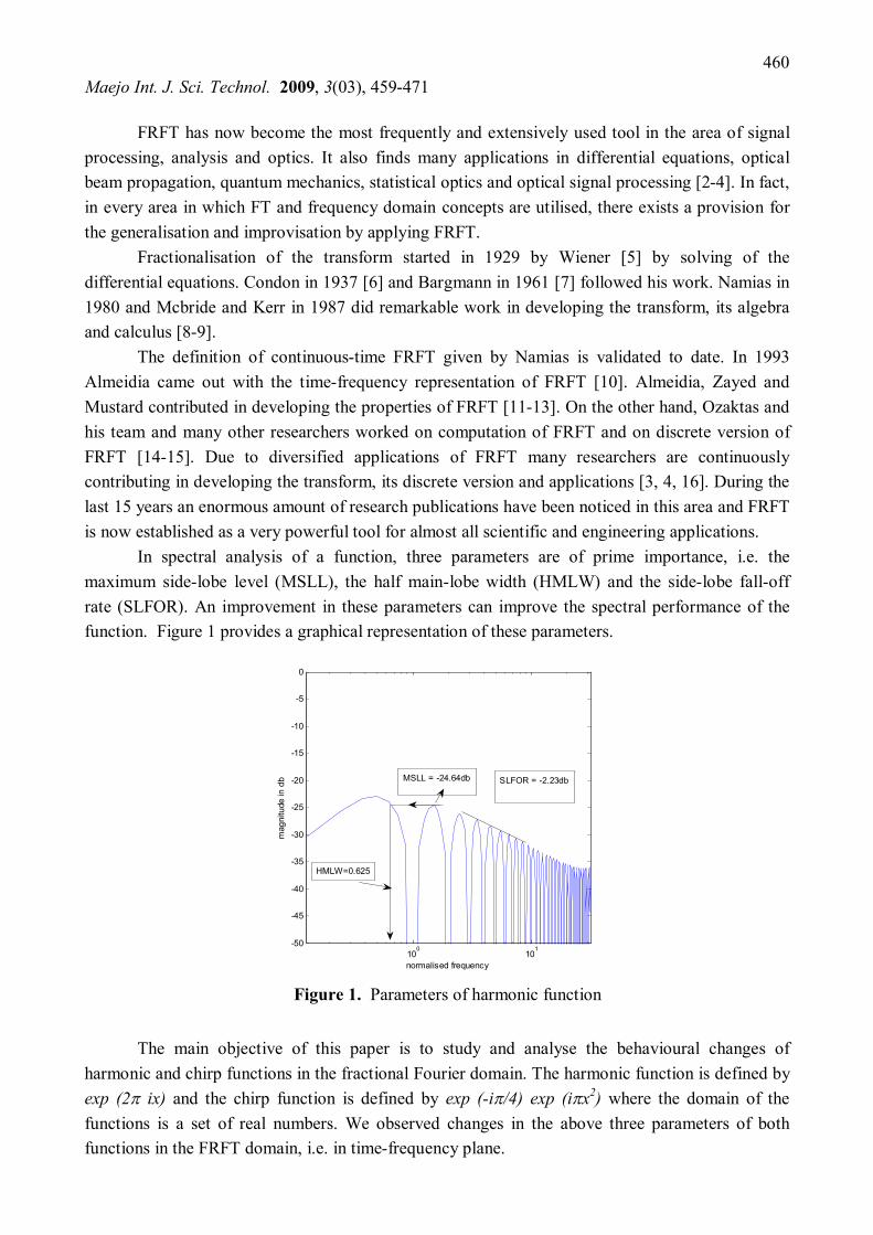
In spectral analysis of a function, three parameters are of prime importance, i.e. the maximum side-lobe level (MSLL), the half main-lobe width (HMLW) and the side-lobe fall-off rate (SLFOR). An improvement in these parameters can improve the spectral performance of the function. Figure 1 provides a graphical representation of these parameters.

100

101

-50

-45

-40

-35

-30

-25

-20

-15

-10

-5

0

normalised frequency

mag

nitu

de in

db MSLL = -24.64db SLFOR = -2.23db

HMLW=0.625

Figure 1. Parameters of harmonic function

The main objective of this paper is to study and analyse the behavioural changes of harmonic and chirp functions in the fractional Fourier domain. The harmonic function is defined by exp (2 ix) and the chirp function is defined by exp (-i/4) exp (ix2) where the domain of the functions is a set of real numbers. We observed changes in the above three parameters of both functions in the FRFT domain, i.e. in time-frequency plane.


461

Defining the Fractional Fourier Transform (FRFT)

The FRFT Fa of order a R is a linear integral operator that maps a given function f(x), x R on to fa ( ).

R by

dx f(x) )x ,(K)(F)(f aa

a

........ (1)

where ) ,( xKa is kernel of transform and defined as follows:

)}cot)x(sin

x(iexp{C)x ,(Ka

222 ........ (2)

with

sin

))//)sgn(sin(iexp(cotiC 241 ........ (3)

where 2 a .

Equation (2) is defined only for a 2 m, i.e. is not a multiple of .

) ,( xK a = m 2 or 4m a for )x( ........ (4)

and ) ,( xKa = 1)(m or 2 4m a for )x( ........ (5)

where m is an integer.

Since 2 a appears in equations only in the argument of trigonometric functions then

the definition is periodic in a (or ) . Thus we will often limit our attention to the interval ],(- or ],(a 22 and sometimes ).2 [0, or ),[a 40 When a is outside the interval

2||0 a we need simply replace a by it’s modulo 4 equivalent.

Different cases can be tabulated, as given in Table 1.

Table 1. Some important cases of FRFT [16]

Operation on signal

Value of parameter

a

Value of 2/ a

Kernel Fractional operator

FT operator 4m + 1 214 /)m( )xiexp( 2 F1 = F Parity operator 4m + 2 )m( 12 )x( F2 = P Identity operator 4m m2 )x( F4m = I Inverse Fourier Transform (IFT) operator

4m +3 234 /)m( )xiexp( 2 F3 = F-1


462

The discrete version of FRFT is known as discrete fractional Fourier transform (DFRFT) and evaluation of FRFT is done by using DFRFT computational techniques [15]. The DFRFT of a signal f(x) can be computed by following four steps: (i) Multiply the function by a chirp (a function whose frequency linearly increases with time), (ii) Take its Fourier transform with its argument scaled by cosec , (iii) Again multiply with a chirp, and (iv) Multiply with a complex constant.

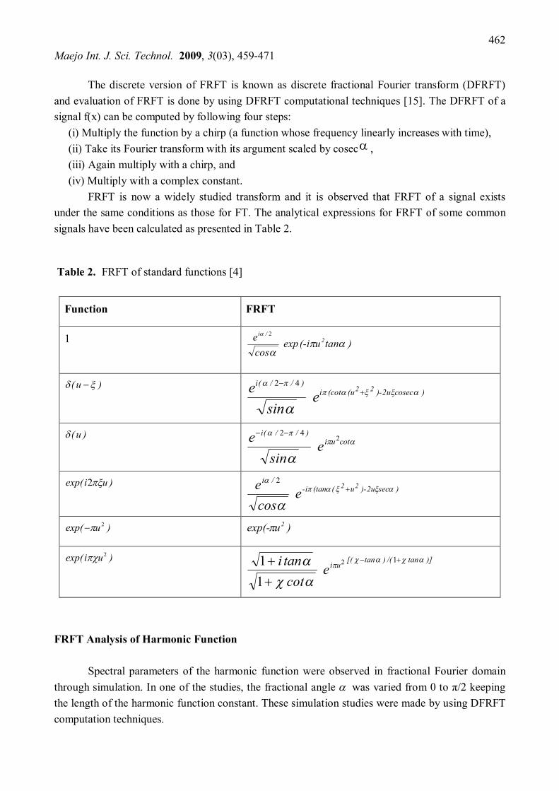
FRFT is now a widely studied transform and it is observed that FRFT of a signal exists under the same conditions as those for FT. The analytical expressions for FRFT of some common signals have been calculated as presented in Table 2.

Table 2. FRFT of standard functions [4]

Function FRFT

1 )tanu(-i exp cose 2

/i

2

)u( )cosec2u-)(u(coti

)//(i22

e sin

e

42

)u(

cotui

)//(i

e sin

e 242

)uiexp( 2 )sec2u-)u((tani-

/i22

e cose

2

)uexp( 2 )uexp(- 2

)uiexp( 2 )]tan/()tan[(uie

cottani

12

11

FRFT Analysis of Harmonic Function

Spectral parameters of the harmonic function were observed in fractional Fourier domain through simulation. In one of the studies, the fractional angle was varied from 0 to π/2 keeping the length of the harmonic function constant. These simulation studies were made by using DFRFT computation techniques.


463

mag

nitu

des

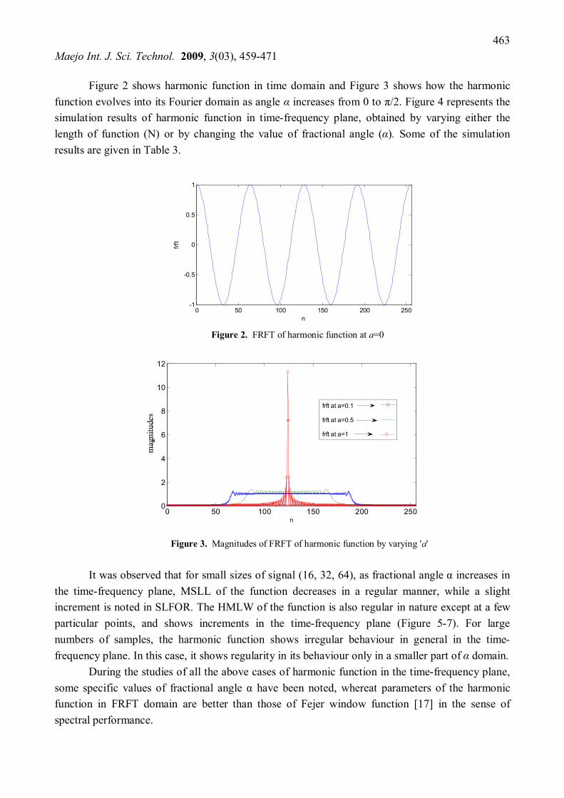
Figure 2 shows harmonic function in time domain and Figure 3 shows how the harmonic function evolves into its Fourier domain as angle α increases from 0 to π/2. Figure 4 represents the simulation results of harmonic function in time-frequency plane, obtained by varying either the length of function (N) or by changing the value of fractional angle (α). Some of the simulation results are given in Table 3.

0 50 100 150 200 250-1

-0.5

0

0.5

1

n

frft

frft of harmonic function at a=0

Figure 2. FRFT of harmonic function at a=0

0 50 100 150 200 2500

2

4

6

8

10

12

n

mag

nitu

des

frft at a=0.1

frft at a=0.5

frft at a=1

Figure 3. Magnitudes of FRFT of harmonic function by varying 'a'

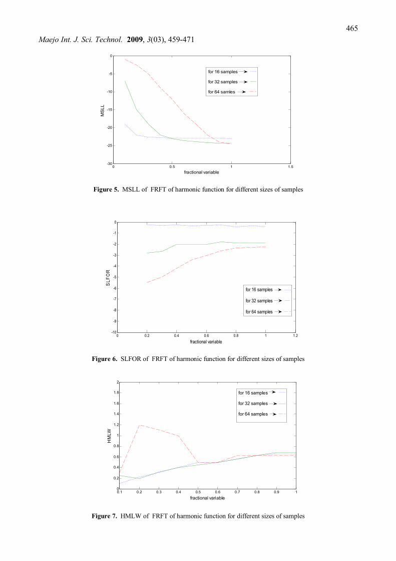
It was observed that for small sizes of signal (16, 32, 64), as fractional angle α increases in

the time-frequency plane, MSLL of the function decreases in a regular manner, while a slight increment is noted in SLFOR. The HMLW of the function is also regular in nature except at a few particular points, and shows increments in the time-frequency plane (Figure 5-7). For large numbers of samples, the harmonic function shows irregular behaviour in general in the time-frequency plane. In this case, it shows regularity in its behaviour only in a smaller part of α domain.

During the studies of all the above cases of harmonic function in the time-frequency plane, some specific values of fractional angle α have been noted, whereat parameters of the harmonic function in FRFT domain are better than those of Fejer window function [17] in the sense of spectral performance.


464

10 -1 10 0 -40

-20

0

m

FRFT of 16 point harmonic function

10 0 10 1 -40

-20

0

m


10 0 10 1 -40

-20

0

m


10 0 10 1 10 2 -40

-20

0

m


10 -1 10 0 10 1 -40

-20

0

m


FRFT at a=0.2

FRFT at a=0.4

FRFT at a=0.6

FRFT at a=0.8

FRFT at a=1

on x-axis - normalised frequency

on y-axis- magnitude of FRFT of harmonicfunction in db (decibel)

Figure 4. FRFT of harmonic function for different sizes of samples

Table 3. Parameters of FRFT of harmonic function

Fractional

angle ‘α’

Sample under

consideration

MSLL in db*

HMLW SLFOR in db*

3π/20 16 -22.68 0.1 -0.30 23π/50 16 -22.98 0.6563 -0.33

π/4 32 -23.16 0.45 -2.04 18π/50 32 -24 0.5625 -1.81 13π/50 64 -12 0.5 -3.42 7π/20 64 -19.2 0.625 -2.58

81π/200 128 -11.7 1.3 -4.5 9π/20 128 -17.32 0.75 -3.03 22π/50 256 -16.5 0.9 -4.2

* = decibel


465

0 0.5 1 1.5-30

-25

-20

-15

-10

-5

0

fractional variable

MS

LL

MSLL of frfts of harmonic function for different sizes of samples

for 16 samples

for 32 samples

for 64 samles

Figure 5. MSLL of FRFT of harmonic function for different sizes of samples

0 0.2 0.4 0.6 0.8 1 1.2-10

-9

-8

-7

-6

-5

-4

-3

-2

-1

0

fractional variable

SLF

OR

SLFOR of frfts of harmonic function for different sizes of samples

for 16 samples

for 32 samples

for 64 samples

Figure 6. SLFOR of FRFT of harmonic function for different sizes of samples

0.1 0.2 0.3 0.4 0.5 0.6 0.7 0.8 0.9 10

0.2

0.4

0.6

0.8

1

1.2

1.4

1.6

1.8

2

fractional variable

HM

LW

for 16 samples

for 32 samples

for 64 samples

Figure 7. HMLW of FRFT of harmonic function for different sizes of samples


466

mag

nitu

des

FRFT Analysis of Chirp Function

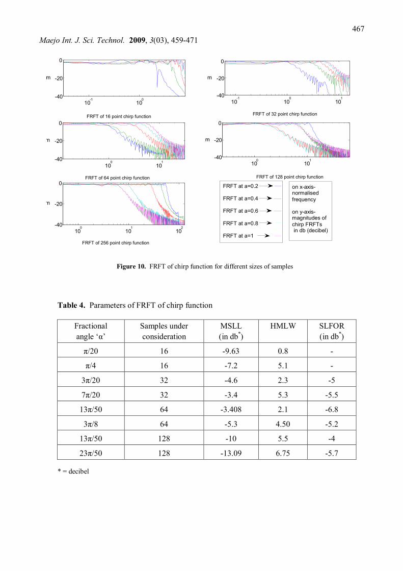
FRFT of the chirp function was obtained and studied through simulation. Figure 8 shows chirp function in time domain while Figure 9 shows how the function transforms from time domain to frequency domain. Figure 10 shows the simulation results. Table 4 represents some of the simulation results for FRFT of a chirp function.

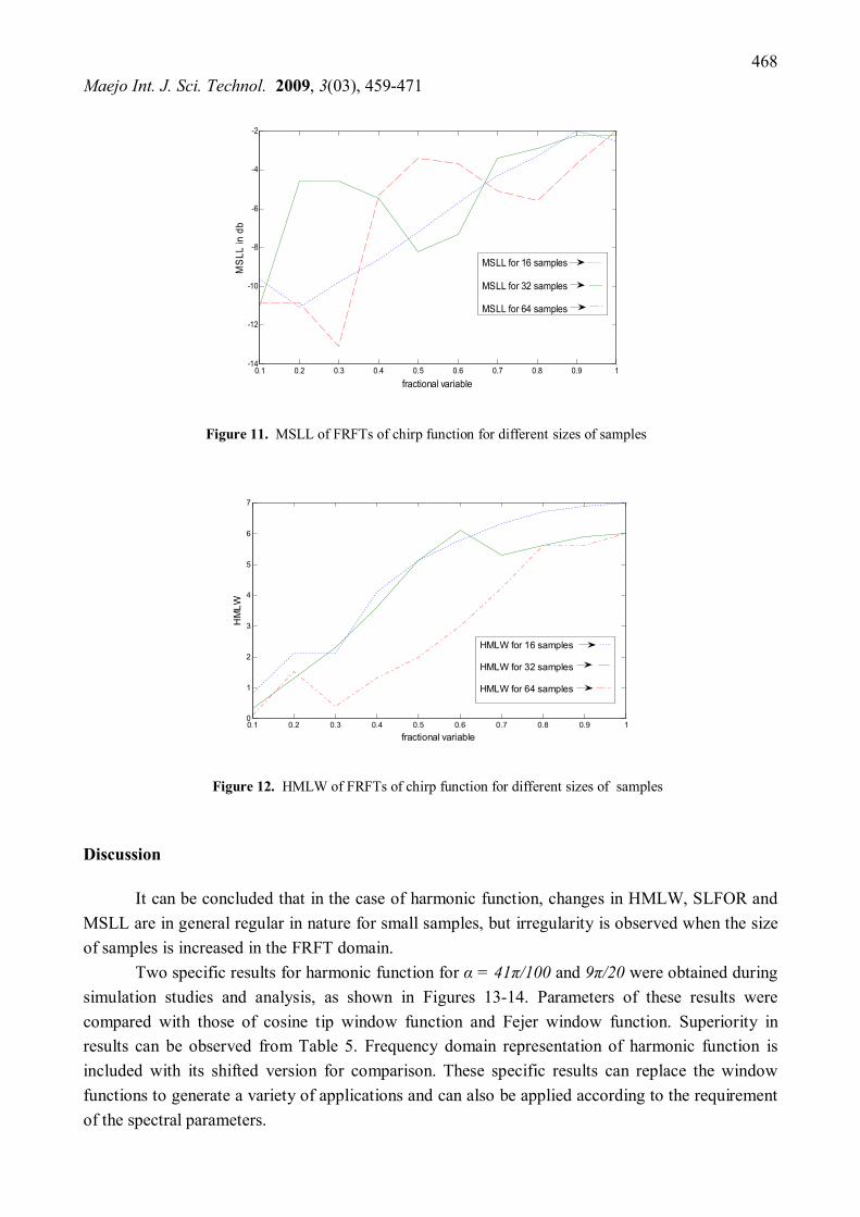
It was observed that in general the chirp function behaves in an irregular manner in time-frequency plane. Figure 10 indicates its nature in α domain for different sizes of samples and Figure 11 shows changes in MSLL of the function in fractional domain. Variation in MSLL increases in α domain when the number of samples is increased. In this case regular increments were noted only in a little part of α domain close to the angle α = π/2.

HMLW of the function in general increases regularly with slight irregular variation for small samples, as shown in Figure12, while SLFOR of the same function also shows variation in an irregular manner but varies between -3 to -6 db. Large numbers of samples produced two specific results as discussed later.

0 10 20 30 40 50 60-1

-0.8

-0.6

-0.4

-0.2

0

0.2

0.4

0.6

0.8

1

n

frft

Figure 8. FRFT of chirp function at a=0

0 50 100 150 200 250 0 0.5

1 1.5

2 2.5

3 3.5

n

gnitude

FRFT at a = 0.2 FRFT at a = 0.5 FRFT at a = 1

Figure 9. Magnitudes of FRFT of chirp function by varying 'a'


467

10 -1 10 0 -40

-20

0

m

FRFT of 16 point chirp function

10 -1 10 0 10 1 -40

-20

0

m


10 0 10 1 10 2 -40

-20

0


m

10 0 10 1 -40

-20

0

m


10 0 10 1 -40

-20

0

m


FRFT at a=0.2 FRFT at a=0.4 FRFT at a=0.6 FRFT at a=0.8 FRFT at a=1

on x-axis- normalised frequency on y-axis- magnitudes of chirp FRFTs in db (decibel)

Figure 10. FRFT of chirp function for different sizes of samples Table 4. Parameters of FRFT of chirp function

Fractional angle ‘α’

Samples under consideration

MSLL (in db*)

HMLW SLFOR (in db*)

π/20 16 -9.63 0.8 -

π/4 16 -7.2 5.1 -

3π/20 32 -4.6 2.3 -5

7π/20 32 -3.4 5.3 -5.5

13π/50 64 -3.408 2.1 -6.8

3π/8 64 -5.3 4.50 -5.2

13π/50 128 -10 5.5 -4

23π/50 128 -13.09 6.75 -5.7

* = decibel


468

0.1 0.2 0.3 0.4 0.5 0.6 0.7 0.8 0.9 1-14

-12

-10

-8

-6

-4

-2

fractional variable

MS

LL in

db

MSLL for 16 samples

MSLL for 32 samples

MSLL for 64 samples

Figure 11. MSLL of FRFTs of chirp function for different sizes of samples

0.1 0.2 0.3 0.4 0.5 0.6 0.7 0.8 0.9 10

1

2

3

4

5

6

7

fractional variable

HM

LW

HMLW for 16 samples

HMLW for 32 samples

HMLW for 64 samples

Figure 12. HMLW of FRFTs of chirp function for different sizes of samples

Discussion

It can be concluded that in the case of harmonic function, changes in HMLW, SLFOR and MSLL are in general regular in nature for small samples, but irregularity is observed when the size of samples is increased in the FRFT domain.

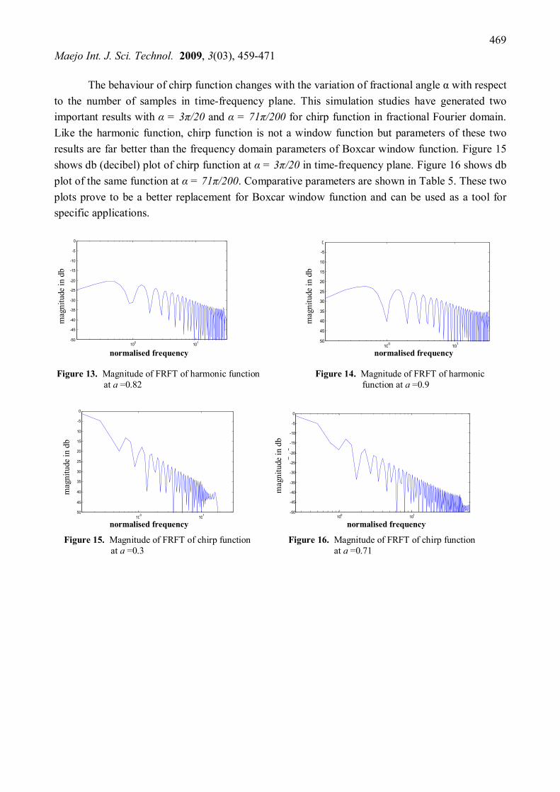
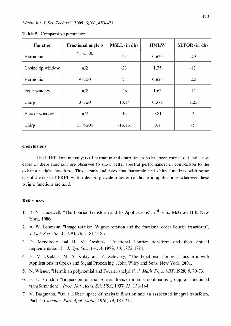
Two specific results for harmonic function for α = 41π/100 and 9π/20 were obtained during simulation studies and analysis, as shown in Figures 13-14. Parameters of these results were compared with those of cosine tip window function and Fejer window function. Superiority in results can be observed from Table 5. Frequency domain representation of harmonic function is included with its shifted version for comparison. These specific results can replace the window functions to generate a variety of applications and can also be applied according to the requirement of the spectral parameters.


469

mag

nitu

de in

db

mag

nitu

de in

db

mag

nitu

de in

db

mag

nitu

de in

db

The behaviour of chirp function changes with the variation of fractional angle α with respect to the number of samples in time-frequency plane. This simulation studies have generated two important results with α = 3π/20 and α = 71π/200 for chirp function in fractional Fourier domain. Like the harmonic function, chirp function is not a window function but parameters of these two results are far better than the frequency domain parameters of Boxcar window function. Figure 15 shows db (decibel) plot of chirp function at α = 3π/20 in time-frequency plane. Figure 16 shows db plot of the same function at α = 71π/200. Comparative parameters are shown in Table 5. These two plots prove to be a better replacement for Boxcar window function and can be used as a tool for specific applications.

10 0 10 1 -50 -45 -40 -35 -30 -25 -20 -15 -10 -5 0

normalised frequency

ma

tud

10 0 10 1 50 45 40 35 30 25 20 15 10 -5 0

normalised frequency normalised frequency Figure 13. Magnitude of FRFT of harmonic function Figure 14. Magnitude of FRFT of harmonic at a =0.82 function at a =0.9

10 0 10 1 50 45 40 35 30 25 20 15 10 -5 0

10 0 10 1 -50 -45 -40 -35 -30 -25 -20 -15 -10 -5 0

ma

tud

normalised frequency normalised frequency

Figure 15. Magnitude of FRFT of chirp function Figure 16. Magnitude of FRFT of chirp function at a =0.3 at a =0.71


470

Table 5. Comparative parameters

Function Fractional angle α MSLL (in db) HMLW SLFOR (in db)

Harmonic 41

-23 0.625 -2.3

Cosine tip window -23 1.35 -12

Harmonic 9 -24 0.625 -2.5

Fejer window -26 1.63 -12

Chirp 3 -13.14 0.375 -5.23

Boxcar window -13 0.81 -6

Chirp 71 -13.16 0.8 -5

Conclusions

The FRFT domain analysis of harmonic and chirp functions has been carried out and a few cases of these functions are observed to show better spectral performances in comparison to the existing weight functions. This clearly indicates that harmonic and chirp functions with some specific values of FRFT with order `a' provide a better candidate in applications wherever these weight functions are used.

References

1. R. N. Bracewell, "The Fourier Transform and Its Applications", 2nd Edn., McGraw Hill, New York, 1986.

2. A. W. Lohmann, "Image rotation, Wigner rotation and the fractional order Fourier transform", J. Opt. Soc. Am. A, 1993, 10, 2181-2186.

3. D. Mendlovic and H. M. Ozaktas, "Fractional Fourier transform and their optical implementation: I", J. Opt. Soc. Am., A, 1993, 10, 1875-1881.

4. H. M. Ozaktas, M. A. Kutay and Z. Zalevsky, "The Fractional Fourier Transform with Applications in Optics and Signal Processing", John Wiley and Sons, New York, 2001.

5. N. Wiener, "Hermitian polynomial and Fourier analysis", J. Math. Phys. MIT, 1929, 8, 70-73.

6. E. U. Condon "Immersion of the Fourier transform in a continuous group of functional transformations", Proc. Nat. Acad. Sci. USA, 1937, 23, 158-164.

7. V. Bargmann, "On a Hilbert space of analytic function and an associated integral transform, Part I", Commun. Pure Appl. Math., 1961, 14, 187-214.


471

8. V. Namias, "The fractional order Fourier transform and its application in quantum mechanics", J. Inst. Math. Applic., 1980, 25, 241-245.

9. A. C. McBride and F. H. Kerr "On Namias's fractional Fourier transform", IMA J. Appl. Math., 1987, 239, 159-175.

10. L. B. Almeida, "The fractional Fourier transform and time frequency representation", IEEE Trans. Signal Process., 1994, 42, 3084-3093.

11. L. B. Almeida, "Product and convolution theorem for the fractional Fourier transform", IEEE Signal Process. Lett., 1997, 4, 15-17.

12. A. I. Zayed, "A convolution and product theorem for the fractional Fourier transform", IEEE Signal Process. Lett., 1998, 5, 101-103.

13. D. Mustard, "Fractional convolution", J. Aust. Math. Soc. Ser. B, 1998, 40, 257-265.

14. H. M. Ozaktas, O. Arikan, M. A. Kutay and G. Bozdagi, "Digital computation of the fractional Fourier transform", IEEE Trans. Signal Process., 1996, 44, 2141-2150.

15. C. Candan, M. A. Kutay and H. M. Ozaktas, "The discrete fractional Fourier transform", IEEE Trans. Signal Process., 2000, 48, 1329-1337.

16. R. Saxena and K. Singh, "Fractional Fourier transform, a novel tool for signal processing", J. Indian Inst. Sci., 2005, 85, 11-26.

17. J. K. Gautam, A. Kumar and R. Saxena "Windows: A tool in signal processing" IETE Tech. Rev., 1995, 12, 217-226.

© 2009 by Maejo University, San Sai, Chiang Mai, 50290 Thailand. Reproduction is permitted for noncommercial purposes.

Maejo Int. J. Sci. Technol. 2009 3(03), 459-471 Maejo ... International Journal of Science and ......

Documents

Transcript of Maejo Int. J. Sci. Technol. 2009 3(03), 459-471 Maejo ... International Journal of Science and ......