Madrid easy

Practical representations of probability sets: aguided tour with applications

Sébastien Destercke

in collaboration with E. Miranda, I. Montes, M. Troffaes, D.Dubois, O. Strauss, C. Baudrit, P.H. Wuillemin.

CNRS researcher, Laboratoire Heudiasyc, Compiègne

Madrid Seminar

Prac Rep 1

Introduction Basics Practical Representations Applications

Plan

l Introduction

l Basics of imprecise probabilities

l A tour of practical representations

l Illustrative applications

Prac Rep 2


Where is Compiegne

Prac Rep 3


Heudiasyc and LABEX MS2T activities

Heudiasycl ' 140 members

l 6M budgetl 4 teams:

m Uncertainty and machinelearning

m Automatic and roboticm Artificial intelligencem Operational research and

networks

LABEX MS2Tl Topic: systems of systemsl 3 laboratories:

m Heudiasycm BMBI: Bio-mechanicm Roberval: mechanic

If interested in collaborations, letme know

Prac Rep 4


Talk in a nutshell

What is this talk about1. (very) Basics of imprecise probability

2. A review of practical representations

3. Some applications

What is this talk not aboutl Deep mathematics of imprecise probabilities (you can ask Nacho or

Quique)

l Imprecise parametric models

Prac Rep 5


Plan

l Introduction




Prac Rep 6


Imprecise probabilities

What?Representing uncertainty as a convex set P of probabilities rather than asingle one

Why?l precise probabilities inadequate to model lack of information;

l generalize set-uncertainty and probabilistic uncertainty;

l can model situations where probabilistic information is partial;

l allow axiomatically alternatives to possibly be incomparable

Prac Rep 7


Probabilities

Probability mass on finite space X = {x1, . . . ,xn} equivalent to a ndimensional vector

p := (p(x1), . . . ,p(xn))

Limited to the set PX of all probabilities

p(x)> 0,∑

x∈X

p(x)= 1 and

The set PX is the (n−1)-unit simplex.

Prac Rep 8


Point in unit simplex

p(x1)= 0.2, p(x2)= 0.5, p(x3)= 0.3

p(x3)

p(x1)

p(x2)

11

1

p(x2)

p(x3) p(x1)

∝ p(X1 )

∝p(x2

)

∝ p(x 3)

Prac Rep 9


Imprecise probability

Set P defined as a set of n constraints

E(fi)≤∑

x∈X

fi(x)p(x)≤ E(fi)

where fi :→R bounded functions

Example2p(x2)−p(x3)≥ 0

f (x1)= 0, f (x2)= 2, f (x3)=−1,E(f )= 0

Lower/upper probabilities

Bounds P(A),P(A) on event A equivalent to

P(A)≤ ∑x∈A

p(x)≤P(A)

Prac Rep 10


Set P example

2p(x2)−p(x3)≥ 0

p(x3)

p(x1)

p(x2)

11

1p(x2)

p(x3) p(x1)

Prac Rep 11


Credal set example

2p(x2)−p(x3)≥ 02p(x1)−p(x2)−p(x3)≥ 0

P

p(x3)

p(x1)

p(x2)

11

1p(x2)

p(x3) p(x1)

Prac Rep 12


Natural extension

From an initial set P defined by constraints, we can compute

l The lower expectation E(g) of any function g as

E(g)= infp∈P

E(g)

l The lower probability P(A) of any event A as

P(A)= infp∈P

P(A)

Prac Rep 13


Some usual problems

l Computing E(g)= infp∈P E(g) of new function g

l Updating P (θ|x)= L(x |θ)P (θ)

l Computing conditional E(f |A)l Simulating/sampling P

l Building joint over variables X1, . . . ,Xn

can be difficult to perform in general → practical representations reducecomputational cost

Prac Rep 14


What makes a representation "practical"

l A reasonable, algorithmically enumerable number of extreme points

reminderp ∈P extreme iff p =λp1 + (1−λ)p2 with λ ∈ (0,1) implies p1 = p2 = p.

We will denote E (P ) the set of extreme points of P

l n-monotone property of P

2-monotonicity (sub-modularity, convexity)

P(A∪B)+P(A∩B)≥P(A)+P(B) for any A,B ⊆X

∞-monotonicity

P(∪ni=1Ai)≥

∑A⊆{A1,...,An}

−1|A|+1P(∪Ai∈A Ai) for any A1, . . . ,An ⊆X and n > 0

Prac Rep 15


Extreme points: illustration

l p(x1)= 1,p(x2)= 0,p(x3)= 0l p(x1)= 0,p(x2)= 1,p(x3)= 0l p(x1)= 0.25,p(x2)= 0.25,p(x3)= 0.5

p(x2)

p(x3) p(x1)

Prac Rep 16


Extreme points: utility

l Computing E(g)→ minimal E on ext. points

l Updating → update extreme points, take convex hull

l Conditional E(f |A) → minimal E(f |A) on ext. points

l Simulating P → take convex mixtures of ext. points

l Joint over variables X1, . . . ,Xn → convex hull of joint extreme

Again, if number of extreme points is limited, or inner approximation (bysampling) acceptable.

Prac Rep 17


2-monotonicity

Computing E(g)Choquet integral

E(g)= infg+∫ supg

infgP({g ≥ t})dt

In finite spaces → sorting n values of g and compute P(A) for n events

Conditioning

P(A|B)= P(A∩B)P(A∩B)+P(Ac ∩B)

And P(A|B) remains 2-monotone (can be used to get E(f |A))

Prac Rep 18


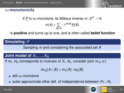
∞-monotonicity

If P is ∞-monotone, its Möbius inverse m : 2X →R

m(A)= ∑B⊆A

−1|A\B|P(B)

is positive and sums up to one, and is often called belief function

Simulating P

Sampling m and considering the associated set A

Joint model of X1, . . . ,XN

If m1,m2 corresponds to inverses of X1,X2, consider joint m12 s.t.

m12(A×B)=m1(A) ·m2(B)

l still ∞-monotone

l outer-approximate other def. of independence between P1, P2

Prac Rep 19


2-monotonicity and extreme points [3]

Generating extreme points if P 2-monotone:

1. Pick a permutation σ : [1,n]→ [1,n] of X

2. Consider sets Aσi = {xσ(1), . . . ,xσ(i)}

3. define Pσ({xσ(i)})=P(Aσi )−P(Aσ

i−1) for i = 1, . . . ,n (Aσ0 =;)

4. then Pσ ∈ E (P )

Some commentsl Maximal value of |E (P )| = n!

l We can have Pσ1 =Pσ2 with σ1 6=σ2 → |E (P )| often less than n!

Prac Rep 20


Example

l X = {x1,x2,x3}

l σ(1)= 2,σ(2)= 3,σ(3)= 1

l Aσ0 =;,Aσ

1 = {x2},Aσ2 = {x2,x3},Aσ

3 =X

l Pσ({xσ(1)})=Pσ({x2})=P({x2})−P(;)=P({x2})

l Pσ({xσ(2)})=Pσ({x3})=P({x2,x3})−P({x2})

l Pσ({xσ(3)})=Pσ({x1})=P(X )−P({x2,x3})= 1−P({x2,x3})

Prac Rep 21


Plan

l Introduction


l A tour of practical representationsm Basicsm Possibility distributionsm P-boxesm Probability intervalsm Elementary Comparative probabilities


Prac Rep 22

Introduction Basics Practical Representations ApplicationsBasics Possibility distributions P-boxes Probability intervals Elem. Compa.

Two very basic models

Probability

l P({xi })=P({xi })=P({xi })

l ∞-monotone, n constraints, |E | = 1

Vacuous model PX

Only support X of probability is known

l P(X )= 1

l ∞-monotone, 1 constraints, |E (P )| = n (Dirac distribution)

Easily extends to vacuous on set A (can be used in robust optimisation,decision under risk, interval-analysis)

Prac Rep 23


A concise graphProbaVacuous

Linear-vacuous Pari-mutuel

Possibilities

P-boxes

Prob. int

Compa.

∞-monotone

2-monotone

Model A

Model B

A special case of B

Prac Rep 24


Neighbourhood models

Build a neighbourhood around a given probability P0

Linear vacuous/ε-contaminationl P(A)= (1−ε)P0(A)+ (ε)PX (A)

l ∞-monotone, n+1 constraints, |E (P )| = n

l ε ∈ [0,1]: unreliability of information P0

Pari-Mutuel [16]l P(A)=max{(1+ε)P0(A)−ε,0}

l 2-monotone, n+1 constraints, |E (P )| =? (n?)

l ε ∈ [0,1]: unreliability of information P0

Other models exist, such as odds-ratio or distance-based (all q s.t. d(p,q)< δ)→ often not attractive for |E (P )|/monotonicity, but may have nice properties(odds/ratio: updating, square/log distances: convex continuous neighbourhood)

Prac Rep 25


Illustration

x2

x3 x1

pari-mutuellinear-vacuous

P0 = (0.5,0.3,0.2)

ε= 0.2

Prac Rep 26




Possibilities

P-boxes

Prob. int

Compa.

∞-monotone

2-monotone

Model A

Model B

A special case of B

Prac Rep 27


Possibility distributions [10]

DefinitionDistribution π :X → [0,1]

with π(x)= 1 for at least one x

P given by

P(A)= minx∈Ac

1−π(x),

which is a necessity measure

π

Characteristics of Pl Necessitates at most n values

l P is an ∞-monotone measure

Prac Rep 28


Possibility distributions

Alternative definitionProvide nested events

A1 ⊆ . . . ⊆An.

Give lower confidence bounds

P(Ai)=αi

with αi+1 ≥αi

Ai

αi

Extreme points [19]

l Maximum number is 2n−1

l Algorithm using nested structure of sets Ai

Prac Rep 29


A basic distribution: simple support

l Set E of most plausiblevalues

l Confidence degree α=P(E)

Extends to multiple sets E1, . . . ,Ep

→ Confidence degrees overnested sets [18]

pH value ∈ [4.5,5.5] with

α= 0.8 (∼ "quite probable")

π

3 4 4.5 5.5 6 70

0.20.40.60.81.0

Prac Rep 30


Partially specified probabilities [1] [8]

Triangular distribution M , [a,b]encompasses all probabilitieswith

l mode/reference value M

l support domain [a,b].

Getting back to pH

l M = 5

l [a,b]= [3,7]

1

pH

π

5 73

Prac Rep 31


Normalized likelihood as possibilities [9] [2]

π(θ)= L(θ|x)/maxθ∗∈ΘL(θ∗|x)

Binomial situation:

l θ = success probability

l x number of observedsuccesses

l x= 4 succ. out of 11

l x= 20 succ. out of 55

θ

1π

4/11

Prac Rep 32


Other examples

l Statistical inequalities (e.g., Chebyshev inequality) [8]

l Linguistic information (fuzzy sets) [5]

l Approaches based on nested models

Prac Rep 33




Possibilities

P-boxes

Prob. int

Compa.

∞-monotone

2-monotone

Model A

Model B

A special case of B

Prac Rep 34


P-boxes [6]

DefinitionWhen X ordered, bounds onevents of the kind:

Ai = {x1, . . . ,xi }

Each bounded by

F (xi)≤P(Ai)≤F (xi)

0.5

1.0

x1 x2 x3 x4 x5 x6 x7

Characteristics of Pl Necessitates at most 2n values

l P is an ∞-monotone measure

Prac Rep 35


In general

DefinitionA set of nested events

A1 ⊆ . . . ⊆An

Each bounded by

αi ≤P(Ai)≤βi

0.5

1.0

x1 x2 x3 x4 x5 x6 x7

Extreme points [15]l At most equal to Pell number Kn = 2Kn−1 +Kn−2

l Algorithm based on a tree structure construction

Prac Rep 36


P-box on reals [11]

A pair [F ,F ] of cumulativedistributions

Bounds over events [−∞,x ]

l Percentiles by experts;

l Kolmogorov-Smirnov bounds;

Can be extended to anypre-ordered space [6], [21] ⇒multivariate spaces!

Expert providing percentiles

0≤P([−∞,12])≤ 0.2

0.2≤P([−∞,24])≤ 0.4

0.6≤P([−∞,36])≤ 0.8

0.5

1.0

6 12 18 24 30 36 42E1

E2

E3

E4

E5

Prac Rep 37




Possibilities

P-boxes

Prob. int

Compa.

∞-monotone

2-monotone

Model A

Model B

A special case of B

Prac Rep 38


Probability intervals [4]

DefinitionElements {x1, . . . ,xn}.

Each bounded by

p(xi) ∈ [p(xi),p(xi)] x1 x2 x3 x4 x5 x6

Characteristics of Pl Necessitates at most 2n values

l P is an 2-monotone measure

Extreme points [4]l Specific algorithm to extract

l If n even, maximum number is(n+1

n/2

)n2

Prac Rep 39


Probability intervals: example

Linguistic assessmentl x is very probable

l x has a good chance

l x is very unlikely

l x probability is about α

⇒Numerical translation

l p(x)≥ 0.75

l 0.4≤ p(x)≤ 0.85

l p(x)≤ 0.25

l α−0.1≤ p(x)≤α+1

Prac Rep 40




Possibilities

P-boxes

Prob. int

Compa.

∞-monotone

2-monotone

Model A

Model B

A special case of B

Prac Rep 41


Comparative probabilities

definitionsComparative probabilities on X : assessments

P(A)≥P(B)

event A "at least as probable as" event B.

Some commentsl studied from the axiomatic point of view [13, 20]

l few studies on their numerical aspects [17]

l interesting for qualitative uncertainty modeling/representation,expert elicitation, . . .

Prac Rep 42


A specific case: elementary comparisons [14]

Elementary comparisonsComparative probability orderings of the states X = {x1, . . . ,xn} in theform of a subset L of {1, . . . ,n}× {1, . . . ,n}.

The set of probability measures compatible with this information is

P (L )= {p ∈PX |∀(i , j) ∈L ,p(xi)≥ p(xj)},

Prac Rep 43


Why focusing on this case?

Practical interestl multinomial models (e.g., imprecise prior for Dirichlet), modal value

elicitation

l direct extension to define imprecise belief functions

Easy to represent/manipulatel Through a graph G = (X ,L ) with states as nodes and relation L

for edges

l Example: given X = {x1, . . . ,x5},L = {(1,3),(1,4),(2,5),(4,5)}, itsassociated graph G is:

x1

x3 x4

x2

x5

Prac Rep 44


Some properties

Characteristics of P

l Necessitates at most n2 values

l No guarantee that P is a 2-monotone measure

Extreme points [14]l Algorithm identifying subsets of disconnected nodes

l maximal number is 2n−1

Prac Rep 45


A concise list (acc. to my knowledge)

Name Monot. Max. |const.| Max. |E (P )| Algo. to get E (P )Proba ∞ n 1 Yes

Vacuous ∞ 1 n Yes2-mon 2 2n n! Yes [3]∞-mon ∞ 2n n! NoLin-vac. ∞ n+1 n Yes

Pari-mutuel 2 n+1 ? (n) NoPossibility ∞ n 2n−1 Yes [19]

P-box (gen.) ∞ 2n Kn (Pell) Yes [15]Prob. int. 2 2n

(n+1n/2

)n2 Yes [4]

Elem. Compa. × n2 2n−1 Yes [14]

Prac Rep 46


A concise final graphProbaVacuous


Possibilities

P-boxes

Prob. int

Compa.

∞-monotone

2-monotone

Model A

Model B

A special case of B

Prac Rep 47


Some open questions

l study the numerical aspects of comparative probabilities withnumbers/general events.

l study the potential link between possibilities and elementarycomparative probabilities (share same number of extreme points,induce ordering between states).

l study restricted bounds/information over specific families of events,other than nested/elementary ones (e.g., events of at most k states).

l look at probability sets induced by bounding specific distances to p0,in particular L1,L2,L∞ norms.

Prac Rep 48


Plan

l Introduction



l Illustrative applicationsm Numerical Signal processing [7]m Camembert ripening [12]

Prac Rep 49

Introduction Basics Practical Representations ApplicationsNumerical filtering Camembert ripening

Signal processing: introduction

l Impulse response µ

filter

µ

l Filtering: convolving kernel µ and observed output f (x)

Prac Rep 50


Link with probability

l If µ positive and∫Rµ(x) dx = 1

l µ equivalent to probability densityl Convolution: compute mathematical expectation Eµ(f )l Numerical filtering: discretize (sampling) µ and f

f f

x0

µ

x0

µ

l µ> 0,∑

xi µ(xi)= 1

Prac Rep 51


Which bandwidth?

Rx

µ

∆???

→ use imprecise probabilistic models to model sets of bandwidth→ possiblities/p-boxes with sets centred around x

Prac Rep 52


Example on simulated signal

time (msec)

signa

l am

plitu

de maxitive upper enveloppe

maxitive lower enveloppe

cloudy upper enveloppe

cloudy lower enveloppe

original signal

Prac Rep 53


Application: pepper/salt noise removal

Original image Noisy image

Prac Rep 54


Results

Zoom on 2 parts

Résultats

CWMF ROAD Us

Prac Rep 55


Motivations

A complex system

The Camembert-type cheese ripening process

tj1 j14Cheese making Cheese ripening (∼ 13◦C, ∼ 95%hum) Warehouse (∼ 4◦C)

P (t = 14

|t = 0

)l Multi-scale modeling; from microbial activities to sensory propertiesl Dynamic probabilistic modell Knowledge is fragmented, heterogeneous and incompletel Difficulties to learn precise model parameters

Use of ε-contamination for a robustness analysis of the model

Prac Rep 56


Experiments

The network

T (t)

Km(t)

lo(t)

Km(t+1)

lo(t+1)

Time slice t Time slice t +1

Unrolled over 14 time steps (days)

T (1)

Km(1)

lo(1)

T (2)

Km(2)

lo(2)

Km(14)

lo(14)

tj1 j14Cheese making Cheese ripening (∼ 13◦C, ∼ 95%hum) Warehouse (∼ 4◦C)

...

Prac Rep 57


Propagation resultsForward propagation, ∀t ∈ �1,τ�,T (t)= 12oC (average ripening room temperature) :

Ext{Km(t)|{Km(1), lo(1),T (1), . . . ,T (τ)}}Ext{lo(t)|{Km(1), lo(1),T (1), . . . ,T (τ)}}

no physical constraints with added physical constraints

Prac Rep 58


Conclusions

Use of practical representationsl +: "Easy" robustness analysis of precise methods, or approximation

of imprecise ones

l +: allow experts to express imprecision or partial information

l +: often easier to explain/represent than general ones

l -: usually focus on specific events

l -: their form may not be conserved by information processing

Prac Rep 59


References I

[1] C. Baudrit and D. Dubois.Practical representations of incomplete probabilistic knowledge.Computational Statistics and Data Analysis, 51(1):86–108, 2006.

[2] M. Cattaneo.Likelihood-based statistical decisions.In Proc. 4th International Symposium on Imprecise Probabilities andTheir Applications, pages 107–116, 2005.

[3] A. Chateauneuf and J.-Y. Jaffray.Some characterizations of lower probabilities and other monotonecapacities through the use of Mobius inversion.Mathematical Social Sciences, 17(3):263–283, 1989.

Prac Rep 60


References II

[4] L. de Campos, J. Huete, and S. Moral.Probability intervals: a tool for uncertain reasoning.I. J. of Uncertainty, Fuzziness and Knowledge-Based Systems,2:167–196, 1994.

[5] G. de Cooman and P. Walley.A possibilistic hierarchical model for behaviour under uncertainty.Theory and Decision, 52:327–374, 2002.

[6] S. Destercke, D. Dubois, and E. Chojnacki.Unifying practical uncertainty representations: I generalizedp-boxes.Int. J. of Approximate Reasoning, 49:649–663, 2008.

Prac Rep 61


References III

[7] S. Destercke and O. Strauss.Filtering with clouds.Soft Computing, 16(5):821–831, 2012.

[8] D. Dubois, L. Foulloy, G. Mauris, and H. Prade.Probability-possibility transformations, triangular fuzzy sets, andprobabilistic inequalities.Reliable Computing, 10:273–297, 2004.

[9] D. Dubois, S. Moral, and H. Prade.A semantics for possibility theory based on likelihoods,.Journal of Mathematical Analysis and Applications, 205(2):359 –380, 1997.

Prac Rep 62


References IV

[10] D. Dubois and H. Prade.Practical methods for constructing possibility distributions.International Journal of Intelligent Systems, 31(3):215–239, 2016.

[11] S. Ferson, L. Ginzburg, V. Kreinovich, D. Myers, and K. Sentz.Constructing probability boxes and dempster-shafer structures.Technical report, Sandia National Laboratories, 2003.

[12] M. Hourbracq, C. Baudrit, P.-H. Wuillemin, and S. Destercke.Dynamic credal networks: introduction and use in robustnessanalysis.In Proceedings of the Eighth International Symposium on ImpreciseProbability: Theories and Applications, pages 159–169, 2013.

Prac Rep 63


References V

[13] B. O. Koopman.The axioms and algebra of intuitive probability.Annals of Mathematics, pages 269–292, 1940.

[14] E. Miranda and S. Destercke.Extreme points of the credal sets generated by comparativeprobabilities.Journal of Mathematical Psychology, 64:44–57, 2015.

[15] I. Montes and S. Destercke.On extreme points of p-boxes and belief functions.In Int. Conf. on Soft Methods in Probability and Statistics (SMPS),2016.

Prac Rep 64


References VI

[16] R. Pelessoni, P. Vicig, and M. Zaffalon.Inference and risk measurement with the pari-mutuel model.International journal of approximate reasoning, 51(9):1145–1158,2010.

[17] G. Regoli.Comparative probability orderings.Technical report, Society for Imprecise Probabilities: Theories andApplications, 1999.

[18] S. Sandri, D. Dubois, and H. Kalfsbeek.Elicitation, assessment and pooling of expert judgments usingpossibility theory.IEEE Trans. on Fuzzy Systems, 3(3):313–335, August 1995.

Prac Rep 65


References VII

[19] G. Schollmeyer.On the number and characterization of the extreme points of thecore of necessity measures on finite spaces.ISIPTA conference, 2016.

[20] P. Suppes, G. Wright, and P. Ayton.Qualitative theory of subjective probability.Subjective probability, pages 17–38, 1994.

[21] M. C. M. Troffaes and S. Destercke.Probability boxes on totally preordered spaces for multivariatemodelling.Int. J. Approx. Reasoning, 52(6):767–791, 2011.

Prac Rep 66

Madrid easy

Science

Transcript of Madrid easy