
Macroeconomics with Heterogeneity: A Practical Guide · F. Guvenen: Macroeconomics with...
73
Economic Quarterly—Volume 97, Number 3—Third Quarter 2011—Pages 255–326 Macroeconomics with Heterogeneity: A Practical Guide Fatih Guvenen What is the origin of inequality among men and is it authorized by natural law? —Academy of Dijon, 1754 (Theme for essay competition) T he quest for the origins of inequality has kept philosophers and sci- entists occupied for centuries. A central question of interest—also highlighted in Academy of Dijon’s solicitation for its essay competi- tion 1 —is whether inequality is determined solely through a natural process or through the interaction of innate differences with man-made institutions and policies. And, if it is the latter, what is the precise relationship between these origins and socioeconomic policies? While many interesting ideas and hypotheses have been put forward over time, the main impediment to progress came from the difficulty of scientifi- cally testing these hypotheses, which would allow researchers to refine ideas that were deemed promising and discard those that were not. Economists, who grapple with the same questions today, have three important advantages that can allow us to make progress. First, modern quantitative economics pro- vides a wide set of powerful tools, which allow researchers to build “laborato- ries” in which various hypotheses regarding the origins and consequences of For helpful discussions, the author thanks Dean Corbae, Cristina De Nardi, Per Krusell, Serdar Ozkan, and Tony Smith. Special thanks to Andreas Hornstein and Kartik Athreya for detailed comments on the draft. David Wiczer and Cloe Ortiz de Mendivil provided excellent research assistance. The views expressed herein are those of the author and not necessarily those of the Federal Reserve Bank of Chicago, the Federal Reserve Bank of Richmond, or the Federal Reserve System. Guvenen is affiliated with the University of Minnesota, the Federal Reserve Bank of Chicago, and NBER. E-mail: [email protected]. 1 The competition generated broad interest from scholars of the time, including Jean-Jacques Rousseau, who wrote his famous Discourse on the Origins of Inequality in response, but failed to win the top prize.
Transcript of Macroeconomics with Heterogeneity: A Practical Guide · F. Guvenen: Macroeconomics with...

Economic Quarterly—Volume 97, Number 3—Third Quarter 2011—Pages 255–326
Macroeconomics withHeterogeneity: A PracticalGuide
Fatih Guvenen
What is the origin of inequality among men and is it authorized bynatural law?
—Academy of Dijon, 1754 (Theme for essay competition)
T he quest for the origins of inequality has kept philosophers and sci-entists occupied for centuries. A central question of interest—alsohighlighted in Academy of Dijon’s solicitation for its essay competi-
tion1—is whether inequality is determined solely through a natural process orthrough the interaction of innate differences with man-made institutions andpolicies. And, if it is the latter, what is the precise relationship between theseorigins and socioeconomic policies?
While many interesting ideas and hypotheses have been put forward overtime, the main impediment to progress came from the difficulty of scientifi-cally testing these hypotheses, which would allow researchers to refine ideasthat were deemed promising and discard those that were not. Economists,who grapple with the same questions today, have three important advantagesthat can allow us to make progress. First, modern quantitative economics pro-vides a wide set of powerful tools, which allow researchers to build “laborato-ries” in which various hypotheses regarding the origins and consequences of
For helpful discussions, the author thanks Dean Corbae, Cristina De Nardi, Per Krusell, SerdarOzkan, and Tony Smith. Special thanks to Andreas Hornstein and Kartik Athreya for detailedcomments on the draft. David Wiczer and Cloe Ortiz de Mendivil provided excellent researchassistance. The views expressed herein are those of the author and not necessarily those ofthe Federal Reserve Bank of Chicago, the Federal Reserve Bank of Richmond, or the FederalReserve System. Guvenen is affiliated with the University of Minnesota, the Federal ReserveBank of Chicago, and NBER. E-mail: [email protected].
1 The competition generated broad interest from scholars of the time, including Jean-JacquesRousseau, who wrote his famous Discourse on the Origins of Inequality in response, but failedto win the top prize.
256 Federal Reserve Bank of Richmond Economic Quarterly
inequality can be studied. Second, the widespread availability of rich micro-data sources—from cross-sectional surveys to panel data sets from adminis-trative records that contain millions of observations—provides fresh input intothese laboratories. Third, thanks to Moore’s law, the cost of computation hasfallen radically in the past decades, making it feasible to numerically solve,simulate, and estimate complex models with rich heterogeneity on a typicaldesktop workstation available to most economists.
There are two broad sets of economic questions for which economistsmight want to model heterogeneity. First, and most obviously, these modelsallow us to study cross-sectional, or distributional, phenomena. The U.S. econ-omy today provides ample motivation for studying distributional issues, withthe top 1 percent of households owning almost half of all stocks and one-thirdof all net worth in the United States, and wage inequality having risen virtuallywithout interruption for the last 40 years. Not surprisingly, many questions ofcurrent policy debate are inherently about their distributional consequences.For example, heated disagreements about major budget issues—such as re-forming Medicare, Medicaid, and the Social Security system—often revolvearound the redistributional effects of such changes. Similarly, a crucial aspectof the current debate on taxation is about “who should pay what?” Answeringthese questions would begin with a sound understanding of the fundamentaldeterminants of different types of inequality.
A second set of questions for which heterogeneity could matter involvesaggregate phenomena. This second use of heterogeneous-agent models is lessobvious than the first, because various aggregation theorems as well as nu-merical results (e.g., Rıos-Rull [1996] and Krusell and Smith [1998]) haveestablished that certain types of heterogeneity do not change (many) implica-tions relative to a representative-agent model.2
To understand this result and its ramifications, in Section 1, I start by re-viewing some key theoretical results on aggregation (Rubinstein 1974;Constantinides 1982). Our interest in these theorems comes from a practi-cal concern: Basically, a subset of the conditions required by these theoremsare often satisfied in heterogeneous-agent models, making the aggregate impli-cations of such models closely mimic those from a representative-agent econ-omy. For example, an important theorem proved by Constantinides (1982)establishes the existence of a representative agent if markets are complete.3
This central role of complete markets turned the spotlight since the late 1980sonto its testable implications for perfect risk sharing (or “full insurance”). As
2 These aggregation results do not imply that all aspects of a representative-agent model willbe the same as those of the underlying individual problem. I discuss important examples to thecontrary in Section 6.
3 (Financial) markets are “complete” when agents have access to a sufficiently rich set ofassets that allows them to transfer their wealth/resources across any two dates and/or states of theworld.

F. Guvenen: Macroeconomics with Heterogeneity 257
I review in Section 2, these implications have been tested by an extensive lit-erature using data sets from all around the world—from developed countriessuch as the United States to village economies in India, Thailand, Uganda,and so on. While this literature delivered a clear statistical rejection, it alsorevealed a surprising amount of “partial” insurance, in the sense that individ-ual consumption growth (or, more generally, marginal utility growth) does notseem to respond to many seemingly large shocks, such as long spells of un-employment, strikes, and involuntary moves (Cochrane [1991] and Townsend[1994], among others).
This raises the more practical question of “how far are we from the com-plete markets benchmark?” To answer this question, researchers have recentlyturned to directly measuring the degree of partial insurance, defined for ourpurposes as the degree of consumption smoothing over and above what anindividual can achieve on her own via “self-insurance” in a permanent incomemodel (i.e., using a single risk-free asset for borrowing and saving). Althoughthis literature is quite new—and so a definitive answer is still not on hand—itis likely to remain an active area of research in the coming years.
The empirical rejection of the complete markets hypothesis launched anenormous literature on incomplete markets models starting in the early 1990s,which I discuss in Section 3. Starting with Imrohoroglu (1989), Huggett(1993), and Aiyagari (1994), this literature has been addressing issues froma very broad spectrum, covering diverse topics such as the equity premiumand other puzzles in finance; important life-cycle choices, such as education,marriage/divorce, housing purchases, fertility choice, etc.; aggregate and dis-tributional effects of a variety of policies ranging from capital and labor incometaxation to the overhaul of Social Security, reforming the health care system,among many others. An especially important set of applications concernstrends in wealth, consumption, and earnings inequality. These are discussedin Section 4.
A critical prerequisite for these analyses is the disentangling of “ex anteheterogeneity” from “risk/uncertainty” (also called ex post heterogeneity)—two sides of the same coin, with potentially very different implications forpolicy and welfare. But this is a challenging task, because inequality of-ten arises from a mixture of heterogeneity and idiosyncratic risk, makingthe two difficult to disentangle. It requires researchers to carefully combinecross-sectional information with sufficiently long time-series data for analy-sis. The state-of-the-art methods used in this field increasingly blend the setof tools developed and used by quantitative macroeconomists with those usedby structural econometricians. Despite the application of these sophisticatedtools, there remains significant uncertainty in the profession regarding themagnitudes of idiosyncratic risks as well as whether or not these risks haveincreased since the 1970s.

258 Federal Reserve Bank of Richmond Economic Quarterly
The Imrohoroglu-Huggett-Aiyagari framework sidestepped a difficult is-sue raised by the lack of aggregation—that aggregates, including prices, de-pend on the entire wealth distribution. This was accomplished by abstractingfrom aggregate shocks, which allowed them to focus on stationary equilibriain which prices (the interest rate and the average wage) were simply someconstants to be solved for in equilibrium. A far more challenging problemwith incomplete markets arises in the presence of aggregate shocks, in whichcase equilibrium prices become functions of the entire wealth distribution,which varies with the aggregate state. Individuals need to know these equi-librium functions so that they can forecast how prices will evolve in the futureas the aggregate state evolves in a stochastic manner. Because the wealthdistribution is an infinite-dimensional object, an exact solution is typically notfeasible. Krusell and Smith (1998) proposed a solution whereby one approx-imates the wealth distribution with a finite number of its moments (inspiredby the idea that a given probability distribution can be represented by itsmoment-generating function). In a remarkable finding, they showed that thefirst moment (the mean) of the wealth distribution was all individuals neededto track in this economy for predicting all future prices. This result—generallyknown as “approximate aggregation”—is a double-edged sword. On the onehand, it makes feasible the solution of a wide range of interesting models withincomplete markets and aggregate shocks. On the other hand, it suggests thatex post heterogeneity does not often generate aggregate implications muchdifferent from a representative-agent model. So, the hope that some aggre-gate phenomena that were puzzling in representative-agent models could beexplained in an incomplete markets framework is weakened with this result.While this is an important finding, there are many examples where hetero-geneity does affect aggregates in a significant way. I discuss a variety of suchexamples in Section 6.
Finally, I turn to computation and calibration. First, in Section 5, I discusssome details of the Krusell-Smith method. A number of potential pitfalls arediscussed and alternative checks of accuracy are studied. Second, an impor-tant practical issue that arises with calibrating/estimating large and complexquantitative models is the following. The objective function that we minimizeoften has lots of jaggedness, small jumps, and/or deep ridges because of a va-riety of reasons that have to do with approximations, interpolations, bindingconstraints, etc. Thus, local optimization methods are typically of little helpon their own, because they very often get stuck in some local minima. In Sec-tion 7, I describe a global optimization algorithm that is simple yet powerfuland is fully parallelizable without requiring any knowledge of MPI, OpenMP,and so on. It works on any number of computers that are connected to theInternet and have access to a synchronization service like DropBox. I pro-vide a discussion of ways to customize this algorithm with different optionsto experiment.

F. Guvenen: Macroeconomics with Heterogeneity 259
1. AGGREGATION
Even in a simple static model with no uncertainty we need a way to deal withconsumer heterogeneity. Adding dynamics and risk into this environmentmakes things more complex and requires a different set of conditions to beimposed. In this section, I will review some key theoretical results on variousforms of aggregation. I begin with a very simple framework and build up toa fully dynamic model with idiosyncratic (i.e., individual-specific) risk anddiscuss what types of aggregation results one can hope to get and under whatconditions.
Our interest in aggregation is not mainly for theoretical reasons. As weshall see, some of the conditions required for aggregation are satisfied (some-times inadvertently!) by commonly used heterogeneous-agent frameworks,making them behave very much like a representative-agent model. Althoughthis often makes the model easier to solve numerically, at the same time itcan make its implications “boring”—i.e., too similar to a representative-agentmodel. Thus, learning about the assumptions underlying the aggregation theo-rems can allow model builders to choose the features of their models carefullyso as to avoid such outcomes.
A Static Economy
Consider a finite setI (with cardinality I ) of consumers who differ in their pref-erences (over l types of goods) and wealth in a static environment. Considera particular good and let xi(p, wi) denote the demand function of consumeri for this good, given prices p ! Rl and wealth wi . Let (w1, w2, ..., wI ) bethe vector of wealth levels for all I consumers. “Aggregate demand” in thiseconomy can be written as
x (p, w1, w2, ..., wI ) =I!
i=1
xi(p, wi).
As seen here, the aggregate demand function x depends on the entirewealth distribution, which is a formidable object to deal with. The key questionthen is, when can we write x(p, w1, w2, ..., wn) " x(p,
"wi)? For the
wealth distribution to not matter, we need aggregate demand to not change forany redistribution of wealth that keeps aggregate wealth constant (
"dwi =
0). Taking the total derivative of x, and setting it to zero yields
!x#p,"
wi
$
!wi
= 0 #n!
i=1
!xi (p, wi)
!wi
dwi = 0
for all possible redistributions. This will only be true if
260 Federal Reserve Bank of Richmond Economic Quarterly
!xi (p, wi)
!wi
= !xj
#p, wj
$
!wj
$i, j ! I.
Thus, the key condition for aggregation is that individuals have the samemarginal propensity to consume (MPC) out of wealth (or linear Engel curves).In one of the earliest works on aggregation, Gorman (1961) formalized thisidea via restrictions on consumers’ indirect utility function, which delivers therequired linearity in Engel curves.
Theorem 1 (Gorman 1961) Consider an economy with N < % commodi-ties and a set I of consumers. Suppose that the preferences of each consumeri ! I can be represented by an indirect utility function4 of the form
vi (p, wi) = ai (p) + b (p) wi,
and that each household i ! I has a positive demand for each commod-ity, then these preferences can be aggregated and represented by those of arepresentative household, with indirect utility
v (p, w) = a (p) + b (p) w,
where a(p) = "i ai(p) and w = "
i wi is aggregate income.
As we shall see later, the importance of linear Engel curves (or constant MPCs)for aggregation is a key insight that carries over to much more general models,all the way up to the infinite-horizon incomplete markets model with aggregateshocks studied in Krusell and Smith (1998).
A Dynamic Economy (No Idiosyncratic Risk)
Rubinstein (1974) extends Gorman’s result to a dynamic economy where in-dividuals consume out of wealth (no income stream). Linear Engel curves areagain central in this context.
Consider a frictionless economy in which each individual solves an in-tertemporal consumption-savings/portfolio allocation problem. That is, everyperiod current wealth wt is apportioned between current consumption ct anda portfolio of a risk-free and a risky security with respective (gross) returnsR
ft and Rs
t .5 Let "t denote the portfolio share of the risk-free asset at time t ,and # denote the subjective time discount factor. Individuals solve
4 Denoting the consumer’s utility function over goods with U , the indirect utility function issimply vi (p, wi) " U(xi(p, wi))—that is, the maximum utility of a consumer who has wealth wiand faces price vector p.
5 We can easily allow for multiple risky securities at the expense of complicating the notation.

F. Guvenen: Macroeconomics with Heterogeneity 261
max{ct ,"t }
E
%T!
t=1
#tU (ct )
&
s.t. wt+1 = (wt & ct )'"tR
ft + (1 & "t ) Rs
t
(.
Furthermore, assume that the period utility function, U , belongs to thehyperbolic absolute risk aversion (HARA) class, which is defined as utilityfunctions that have linear risk tolerance: T (c) " &U(c)'/U(c)'' = $+% c and% < 1.6 This class encompasses three utility functions that are well-knownin economics: U(c) = (% & 1)&1($ + % c)1&%&1
(generalized power utility;standard constant relative risk aversion [CRRA] form when $ " 0); U(c) =&$ ( exp(&c/$) if % " 0 (exponential utility); and U(c) = 0.5($ & c)2
defined for values c < $ (quadratic utility).The following theorem gives six sets of conditions under which aggrega-
tion obtains.7
Theorem 2 (Rubenstein 1974) Consider the following homogeneityconditions:
1. All individuals have the same resources w0, and tastes # and U .2. All individuals have the same # and taste parameters % )= 0.3. All individuals have the same taste parameters % = 0.4. All individuals have the same resources w0 and taste parameters $ = 0
and % = 1.5. A complete market exists and all individuals have the same taste pa-
rameter % = 0.6. A complete market exists and all individuals have the same resources
w0 and taste #, $ = 0, and % = 1.Then, all equilibrium rates of return are determined in case (1) as if there
exist only composite individuals each with resources w0 and tastes # and U ;and equilibrium rates of return are determined in cases (2)–(6) as if thereexist only composite individuals each with the following economic character-istics: (i) resources: w0 = "
wi0/I ; (ii) tastes: & = '(& i)($i /
"$i ) (where
& " 1/# & 1) or # = "#i/I ; and (iv) preference parameters: $ = "
$i/I ,and % .
Several remarks are in order.
6 “Risk tolerance” is the reciprocal of the Arrow-Pratt measure of “absolute risk aversion,”which measures consumers’ willingness to bear a fixed amount of consumption risk. See, e.g.,Pratt (1964).
7 The language of Theorem 2 differs from Rubinstein’s original statement by assuming rationalexpectations and combines results with the extension to a multiperiod setting in his footnote 5.

262 Federal Reserve Bank of Richmond Economic Quarterly
Demand Aggregation
An important corollary to this theorem is that whenever a composite consumercan be constructed, in equilibrium, rates of return are insensitive to the distri-bution of resources among individuals. This is because the aggregate demandfunctions (for both consumption and assets) depend only on total wealth andnot on its distribution. Thus, we have “demand aggregation.”
Aggregation and Heterogeneity in Relative Risk Aversion
Notice that all six cases that give rise to demand aggregation in the theoremrequire individuals to have the same curvature parameter, % . To see why thisis important, note that (with HARA preferences) the optimal holdings of therisky asset are a linear function of the consumer’s wealth: (1 +(2wt/% , where(1 and (2 are some constants that depend on the properties of returns. It is easyto see that with identical slopes, (2
%, it does not matter who holds the wealth.
In other words, redistributing wealth between any two agents would causechanges in total demand for assets that will cancel out each other, becauseof linearity and same slopes. Notice also that while identical curvature is anecessary condition, it is not sufficient for demand aggregation: Each of thesix cases adds more conditions on top of this identical curvature requirement.8
A Dynamic Economy (With Idiosyncratic Risk)
While Rubinstein’s (1974) theorem delivers a strong aggregation result, itachieves this by abstracting from a key aspect of dynamic economies: un-certainty that evolves over time. Almost every interesting economy that wediscuss in the coming sections will feature some kind of idiosyncratic risk thatindividuals face (coming from labor income fluctuations, shocks to health,shocks to housing prices and asset returns, among others). Rubinstein’s(1974) theorem is silent about how the aggregate economy behaves under thesescenarios.
This is where Constantinides (1982) comes into play: He shows that ifmarkets are complete, under much weaker conditions (on preferences, beliefs,discount rates, etc.) one can replace heterogeneous consumers with a plannerwho maximizes a weighted sum of consumers’ utilities. In turn, the centralplanner can be replaced by a composite consumer who maximizes a utilityfunction of aggregate consumption.
To show this, consider a private ownership economy with production as inDebreu (1959), with m consumers, n firms, and l commodities. As in Debreu
8 Notice also that, because in some cases (such as [2]) heterogeneity in $ is allowed, indi-viduals will exhibit different relative risk aversions (if they have different wt ), for example in thegeneralized CRRA case, and still allow aggregation.
F. Guvenen: Macroeconomics with Heterogeneity 263
(1959), these commodities can be thought of as date-event labelled goods (andconcave utility functions, Ui , as being defined over these goods), allowing us tomap these results into an intertemporal economy with uncertainty. Consumer iis endowed with wealth (wi1, wi2, ..., wil) and shares of firms () i1, ) i2, ..., ) in)with ) ij * 0 and
"m ) ij = 1. Let the vectors Ci and Yj denote, respectively,
individual i’s consumption set and firm j ’s production set.An equilibrium is an (m+n+1)-tuple ((c+
i )mi=1, (y
+j )
nj=1, p
+) such that, asusual, consumers maximize utility, firms maximize their profits, and marketsclear. Under standard assumptions, an equilibrium exists and is Pareto optimal.
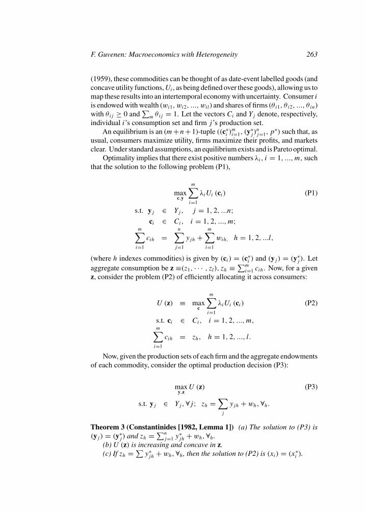
Optimality implies that there exist positive numbers *i , i = 1, ..., m, suchthat the solution to the following problem (P1),
maxc,y
m!
i=1
*iUi (ci) (P1)
s.t. yj ! Yj , j = 1, 2, ...n;ci ! Ci, i = 1, 2, ..., m;
m!
i=1
cih =n!
j=1
yjh +m!
i=1
wih, h = 1, 2, ...l,
(where h indexes commodities) is given by (ci) = (c+i ) and (yj ) = (y+
j ). Letaggregate consumption be z "(z1, · · · , zl), zh " "m
i=1 cih. Now, for a givenz, consider the problem (P2) of efficiently allocating it across consumers:
U (z) " maxc
m!
i=1
*iUi (ci) (P2)
s.t. ci ! Ci, i = 1, 2, ..., m,m!
i=1
cih = zh, h = 1, 2, ..., l.
Now, given the production sets of each firm and the aggregate endowmentsof each commodity, consider the optimal production decision (P3):
maxy,z
U (z) (P3)
s.t. yj ! Yj , $j ; zh =!
j
yjh + wh, $h.
Theorem 3 (Constantinides [1982, Lemma 1]) (a) The solution to (P3) is(yj ) = (y+
j ) and zh = "nj=1 y+
jh + wh, $h.(b) U (z) is increasing and concave in z.(c) If zh = "
y+jh + wh, $h, then the solution to (P2) is (xi) = (x+
i ).
264 Federal Reserve Bank of Richmond Economic Quarterly
(d) Given *i , i = 1, 2, · · · , m, then if the consumers are replaced byone composite consumer with utility U (z), with endowment equal to the sumof m consumers’ endowments and shares the sum of their shares, then the(1 + n + 1)-tuple (
"mi=1 c+
i , (y+j )
nj=1, p
+) is an equilibrium.
Constantinides versus Rubinstein
Constantinides allows for much more generality than Rubinstein by relax-ing two important restrictions. First, no conditions are imposed on the ho-mogeneity of preferences, which was a crucial element in every version ofRubinstein’s theorem. Second, Constantinides allows for both exogenousendowment as well as production at every date and state. In contrast, re-call that, in Rubinstein’s environment, individuals start life with a wealthstock and receive no further income or endowment during life. In exchange,Constantinides requires complete markets and does not get demand aggrega-tion. Notice that the existence of a composite consumer does not imply demandaggregation, for at least two reasons. First, composite demand depends on theweights in the planner’s problem and, thus, depends on the distribution of en-dowments. Second, the composite consumer is defined at equilibrium pricesand there is no presumption that its demand curve is identical to the aggregatedemand function.
Thus, the usefulness of Constantinides’s result hinges on (i) the degree towhich markets are complete, (ii) whether we want to allow for idiosyncraticrisk and heterogeneity in preferences (which are both restricted in Rubinstein’stheorem), and (iii) whether or not we need demand aggregation. Below I willaddress these issues in more detail. We will see that, interestingly, even whenmarkets are not complete, in certain cases, we will not only get close to a com-posite consumer representation, but we can also get quite close to the muchstronger result of demand aggregation! An important reason for this outcomeis that many heterogeneous-agent models assume identical preferences, whicheliminates an important source of heterogeneity, satisfying Rubinstein’s con-ditions for preferences. While these models do feature idiosyncratic risk, aswe shall see, when the planning horizon is long such shocks can often besmoothed effectively using even a simple risk-free asset. More on this in thecoming sections.
Completing Markets by Adding Financial Assets
It is useful to distinguish between “physical” assets—those in positive netsupply (e.g., equity shares, capital, housing, etc.)—and “financial” assets—those in zero net supply (bonds, insurance contracts, etc.). The latter are simplysome contracts written on a piece of paper that specify the conditions underwhich one agent transfers resources to another. In principle, it can be createdwith little cost. Now suppose that we live in a world with J physical assets and

F. Guvenen: Macroeconomics with Heterogeneity 265
that there are S(> J) states of the world. In this general setting, markets areincomplete. However, if consumers have homogenous tastes, endowments,and beliefs, then markets are (effectively) complete by simply adding enoughfinancial assets (in zero net supply). There is no loss of optimality and nothingwill change by this action, because in equilibrium identical agents will nottrade with each other. The bottom line is that the more “homogeneity” weare willing to assume among consumers, the less demanding the completemarkets assumption becomes. This point should be kept in mind as we willreturn to it later.
2. EMPIRICAL EVIDENCE ON INSURANCE
Dynamic economic models with heterogeneity typically feature individual-specific uncertainty that evolves over time—coming from fluctuations inlabor earnings, health status, portfolio returns, among others. Although thisstructure does not fit into Rubinstein’s environment, it is covered byConstantinides’s theorem, which requires complete markets. Thus, a keyempirical question is the extent to which complete markets can serve as auseful benchmark and a good approximation to the world we live in. As weshall see in this section, the answer turns out to be more nuanced than a simpleyes or no.
To explain the broad variety of evidence that has been brought to bear onthis question, this section is structured in the following way. First, I beginby discussing a large empirical literature that has tested a key prediction ofcomplete markets—that marginal utility growth is equated across individuals.This is often called “perfect” or “full” insurance, and it is soundly rejected inthe data. Next, I discuss an alternative benchmark, inspired by this rejection.This is the permanent income model, in which individuals have access toonly borrowing and saving—or “self-insurance.” In a way, this is the otherextreme end of the insurance spectrum. Finally, I discuss studies that takean intermediate view—“partial insurance”—and provide some evidence tosupport it. We now begin with the tests of full insurance.
Benchmark 1: Full Insurance
To develop the theoretical framework underlying the empirical analyses, startwith an economy populated by agents who derive utility from consumption ct
as well as some other good(s) dt : Ui#cit+1, d
it+1
$, where i indexes individuals.
These other goods can include leisure time (of husband and wife if the unit ofanalysis is a household), children, lagged consumption (as in habit formationmodels), and so on.
The key implication of perfect insurance can be derived by following twodistinct approaches. The first environment assumes a social planner who pools

266 Federal Reserve Bank of Richmond Economic Quarterly
all individuals’ resources and maximizes a social welfare function that assignsa positive weight to every individual. In the second environment, allocationsare determined in a competitive equilibrium of a frictionless economy whereindividuals are able to trade in a complete set of financial securities. Both ofthese frameworks make the following strong prediction for the growth rate ofindividuals’ marginal utilities:
#iU i
c
#cit+1, d
it+1
$
Uic
#cit , d
it
$ = +t+1
+t
, (1)
where Uc denotes the marginal utility of consumption and +t is the aggre-gate shock.9 Thus, this condition says that every individual’s marginal utilitymust grow in locksteps with the aggregate and, hence, with each other. Noindividual-specific term appears on the right-hand side, such as idiosyncraticincome shocks, unemployment, sickness, and so on. All these idiosyncraticevents are perfectly insured in this world. From here one can introduce anumber of additional assumptions for empirical tractability.
Complete Markets and Cross-Sectional Heterogeneity:A Digression
So far we have focused on what market completeness implies for the study ofaggregate phenomena in light of Constantinides’s theorem. However, com-plete markets also imposes restrictions on the evolution of the cross-sectionaldistribution, which can be seen in (1). For a given specification of U , (1)translates into restrictions on the evolutions of ct and dt (possibly a vector).Although it is possible to choose U to be sufficiently general and flexible(e.g., include preference shifters, assume non-separability) to generate richdynamics in cross-sectional distributions, this strategy would attribute all theaction to preferences, which are essentially unobservable. Even in that case,models that are not bound by (1)—and therefore have idiosyncratic shocks af-fect individual allocations—can generate a much richer set of cross-sectionaldistributions. Whether that extra richness is necessary for explaining salientfeatures of the data is another matter and is not always obvious (see, e.g.,Caselli and Ventura [2000], Badel and Huggett [2007], and Guvenen andKuruscu [2010]).10
9 Alternatively stated, +t is the Lagrange multiplier on the aggregate resource constraintat time t in the planner’s problem or the state price density in the competitive equilibriuminterpretation.
10 Caselli and Ventura (2000) show that a wide range of distributional dynamics and incomemobility patterns can arise in the Cass-Koopmans optimal savings model and in the Arrow-Romermodel of productivity spillovers. Badel and Huggett (2007) show that life-cycle inequality patterns(discussed later) that have been viewed as evidence of incomplete markets can in fact be generatedusing a complete markets model. Guvenen and Kuruscu (2010) show that a human capital modelwith heterogeneity in learning ability and skill-biased technical change generates rich nonmonotonic

F. Guvenen: Macroeconomics with Heterogeneity 267
Now I return back to the empirical tests of (1).In a pioneering article, Altug and Miller (1990) were the first to formally
test the implications of (1). They considered households as their unit of analy-sis and specified a rich Beckerian utility function that included husbands’ andwives’ leisure times as well as consumption (food expenditures), and adjustedfor demographics (children, age, etc.). Using data from the Panel Study ofIncome Dynamics (PSID), they could not reject full insurance. Hayashi,Altonji, and Kotlikoff (1996) revisited this topic a few years later and, usingthe same data set, they rejected perfect risk sharing.11 Given this rejectionin the whole population, they investigated if there might be better insurancewithin families, who presumably have closer ties with each other than thepopulation at large and could therefore provide insurance to the members inneed. They found that this hypothesis too was statistically rejected.12
In a similar vein, Guvenen (2007a) investigates how the extent of risksharing varies across different wealth groups, such as stockholders and non-stockholders. This question is motivated by the observation that stockholders(who made up less than 20 percent of the population for much of the 20thcentury) own about 80 percent of net worth and 90 percent of financial wealthin the U.S. economy, and therefore play a disproportionately large role in thedetermination of macroeconomic aggregates. On the one hand, these wealthyindividuals have access to a wide range of financial securities that can pre-sumably allow better risk insurance; on the other hand, they are exposed todifferent risks not faced by the less-wealthy nonstockholders. Using data fromthe PSID, he strongly rejects perfect risk sharing among stockholders, but, per-haps surprisingly, does not find evidence against it among nonstockholders.This finding suggests further focus on risk factors that primarily affect thewealthy, such as entrepreneurial income risk that is concentrated at the top ofthe wealth distribution.
A number of other articles impose further assumptions before testing forrisk sharing. A very common assumption is the separability between ct and dt
(for example, leisure), which leads to an equation that only involves consump-tion (Cochrane 1991, Nelson 1994, Attanasio and Davis 1996).13 Assumingpower utility in addition to separability, we can take the logs of both sides of
dynamics consistent with the U.S. data since the 1970s, despite featuring no idiosyncratic shocks(and thus has complete markets).
11 Data sets such as the PSID are known to go through regular revisions, which might beable to account for the discrepancy between the two articles’ results.
12 This finding has implications for the modeling of the household decision-making processas a unitary model as opposed to one in which there is bargaining between spouses.
13 Non-separability, for example between consumption and leisure, can be allowed for if theplanner is assumed to be able to transfer leisure freely across individuals. While transfers ofconsumption are easier to implement (through taxes and transfers), the transfer of leisure is harderto defend on empirical grounds.

268 Federal Reserve Bank of Richmond Economic Quarterly
equation (1) and then time-difference to obtain
,Ci,t = ,+t , (2)
where Ct " log(ct ) and ,Ct " Ct & Ct&1. Several articles have tested thisprediction by running a regression of the form
,Ci,t = ,+t +- 'Zit + .i,t , (3)
where the vector Zit contains factors that are idiosyncratic to individual/
household/group i. Perfect insurance implies that all the elements of thevector - are equal to zero.
Cochrane (1991), Mace (1991), and Nelson (1994) are the early studiesthat exploit this simple regression structure. Mace (1991) focuses on whetheror not consumption responds to idiosyncratic wage shocks, i.e., Zi
t = ,Wit .14
While Mace fails to reject full insurance, Nelson (1994) later points out severalissues with the treatment of data (and measurement error in particular) thataffect Mace’s results. Nelson shows that a more careful treatment of theseissues results in strong rejection.
Cochrane (1991) raises a different point. He argues that studies suchas Mace’s, that test risk sharing by examining the response of consumptiongrowth to income, may have low power if income changes are (at least partly)anticipated by individuals. He instead proposes to use idiosyncratic eventsthat are arguably harder to predict, such as plant closures, long strikes, longillnesses, and so on. Cochrane rejects full insurance for illness or involuntaryjob loss but not for long spells of unemployment, strikes, or involuntary moves.Notice that a crucial assumption in all of the work of this kind is that noneof these shocks can be correlated with unmeasured factors that determinemarginal utility growth.
Townsend (1994) tests for risk sharing in village economies of India andconcludes that, although the model is statistically rejected, full insurance pro-vides a surprisingly good benchmark. Specifically, he finds that individualconsumption co-moves with village-level consumption and is not influencedmuch by own income, sickness, and unemployment.
Attanasio and Davis (1996) observe that equation (2) must also hold formultiyear changes in consumption and when aggregated across groups ofindividuals.15 This implies, for example, that even if one group of individualsexperiences faster income growth relative to another group during a 10-yearperiod, their consumption growth must be the same. The substantial rise in theeducation premium in the United States (i.e., the wages of college graduates
14 Because individual wages are measured with (often substantial) error in microsurvey datasets, an ordinary least squares estimation of this regression would suffer from attenuation bias,which may lead to a failure to reject full insurance even when it is false. The articles discussedhere employ different approaches to deal with this issue (such as using an instrumental variablesregression or averaging across groups to average out measurement error).
15 Hayashi, Altonji, and Kotlikoff (1996) also use multiyear changes to test for risk sharing.
F. Guvenen: Macroeconomics with Heterogeneity 269
relative to high school graduates) throughout the 1980s provided a key test ofperfect risk sharing. Contrary to this hypothesis, Attanasio and Davis (1996)find that the consumption of college graduates grows much faster than that ofhigh school graduates during the same period, violating the premise of perfectrisk sharing.
Finally, Schulhofer-Wohl (2011) sheds new light on this question. Heargues that if more risk-tolerant individuals self-select into occupations withmore (aggregate) income risk, then the regressions in (3) used by Cochrane(1991), Nelson (1994), and others (which incorrectly assume away such cor-relation) will be biased toward rejecting perfect risk sharing. By using self-reported measures of risk attitudes from the Health and Retirement Survey,Schulhofer-Wohl establishes such a correlation. Then he develops a methodto deal with this bias and, applying the corrected regression, he finds thatconsumption growth responds very weakly to idiosyncratic shocks, implyingmuch larger risk sharing than can be found in these previous articles. He alsoshows that the coefficients estimated from this regression can be mapped intoa measure of “partial insurance.”
Taking Stock
As the preceding discussion makes clear, with few exceptions, all empiricalstudies agree that perfect insurance in the whole population is strongly rejectedin a statistical sense. However, this statistical rejection per se is not sufficientto conclude that complete markets is a poor benchmark for economic analysisfor two reasons. First, there seems to be a fair deal of insurance againstcertain types of shocks, as documented by Cochrane (1991) and Townsend(1994), and among certain groups of households, such as in some villagesin less developed countries (Townsend 1994), or among nonstockholders inthe United States (Guvenen 2007a). Second, the reviewed empirical evidencearguably documents statistical tests of an extreme benchmark (equation [1])that we should not expect to hold precisely—for every household, against everyshock. Thus, with a large enough sample, statistical rejection should not besurprising.16 What these tests do not do is tell us how “far” the economy is fromthe perfect insurance benchmark. In this sense, analyses such as in Townsend(1994)—that identify the types of shocks that are and are not insured—aresomewhat more informative than those in Altug and Miller (1990), Hayashi,Altonji, and Kotlikoff (1996), and Guvenen (2007a), which rely on modelmisspecification-type tests of risk sharing.
16 One view is that hypothesis tests without an explicit alternative (such as the ones dis-cussed here) often “degenerate into elaborate rituals designed to measure the sample size (Leamer1983, 39).”
270 Federal Reserve Bank of Richmond Economic Quarterly
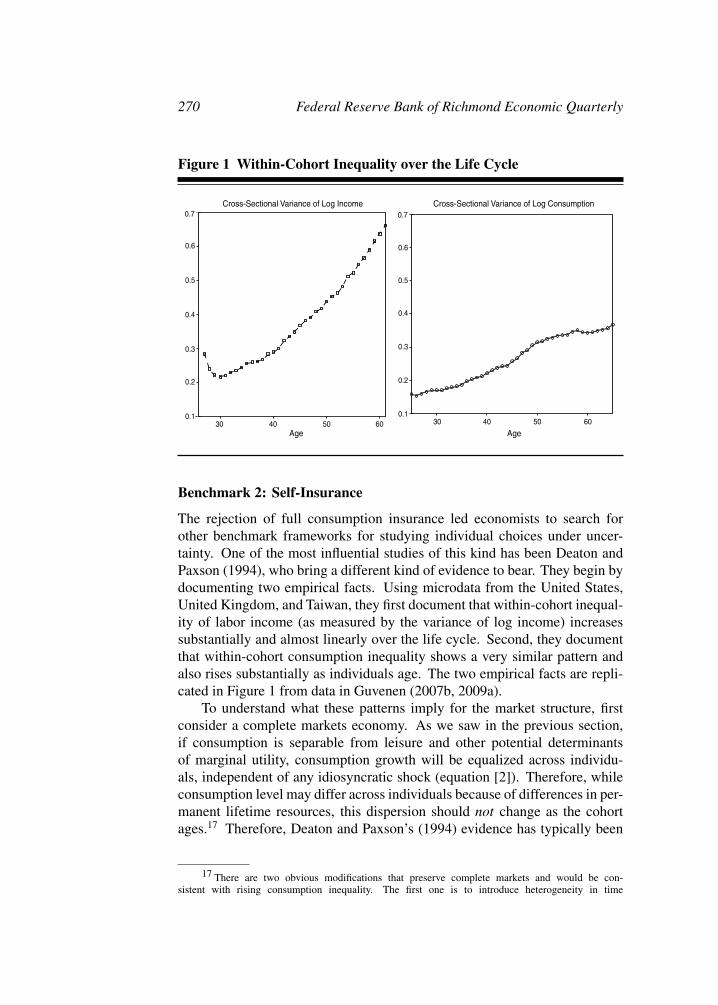
Figure 1 Within-Cohort Inequality over the Life Cycle
Cross-Sectional Variance of Log Income Cross-Sectional Variance of Log Consumption
Age Age30 40 50 60 30 40 50 60
0.1
0.2
0.3
0.4
0.5
0.6
0.7
0.1
0.2
0.3
0.4
0.5
0.6
0.7
Benchmark 2: Self-Insurance
The rejection of full consumption insurance led economists to search forother benchmark frameworks for studying individual choices under uncer-tainty. One of the most influential studies of this kind has been Deaton andPaxson (1994), who bring a different kind of evidence to bear. They begin bydocumenting two empirical facts. Using microdata from the United States,United Kingdom, and Taiwan, they first document that within-cohort inequal-ity of labor income (as measured by the variance of log income) increasessubstantially and almost linearly over the life cycle. Second, they documentthat within-cohort consumption inequality shows a very similar pattern andalso rises substantially as individuals age. The two empirical facts are repli-cated in Figure 1 from data in Guvenen (2007b, 2009a).
To understand what these patterns imply for the market structure, firstconsider a complete markets economy. As we saw in the previous section,if consumption is separable from leisure and other potential determinantsof marginal utility, consumption growth will be equalized across individu-als, independent of any idiosyncratic shock (equation [2]). Therefore, whileconsumption level may differ across individuals because of differences in per-manent lifetime resources, this dispersion should not change as the cohortages.17 Therefore, Deaton and Paxson’s (1994) evidence has typically been
17 There are two obvious modifications that preserve complete markets and would be con-sistent with rising consumption inequality. The first one is to introduce heterogeneity in time
F. Guvenen: Macroeconomics with Heterogeneity 271
interpreted as contradicting the complete markets framework. I now turn tothe details.
The Permanent Income Model
The canonical framework for self-insurance is provided by the permanent in-come life-cycle model, in which individuals only have access to a risk-freeasset for borrowing and saving. Therefore, as opposed to full insurance, thereis only “self-insurance” in this framework. Whereas the complete marketsframework represents the maximum amount of insurance, the permanent in-come model arguably provides the lower bound on insurance (to the extentthat we believe individuals have access to a savings technology, and borrowingis possible subject to some constraints).
It is instructive to develop this framework in some detail as the resultingequations will come in handy in the subsequent exposition. The frameworkhere closely follows Hall and Mishkin (1982) and Deaton and Paxson (1994).Start with an income process with permanent and transitory shocks:
yt = yPt + /t ,
yPt = yP
t&1 + 0t . (4)
Suppose that individuals discount the future at the rate of interest anddefine: # = 1/(1 + r). Preferences are of quadratic utility form:
max E0
)
&12
T!
t=1
#t
#c+ & ct
$2
*
s.t.T!
t=1
#t (yt & ct ) + A0 = 0, (5)
where c+ is the bliss level and A0 is the initial wealth level (which may bezero). This problem can be solved in closed form to obtain a consumptionfunction. First-differencing this consumption rule yields
,ct = 0t + % t/t , (6)
where % t " 1/'"T &t
1=0 #1(
is the annuitization factor.18 This term is closeto zero when the horizon is long and the interest rate is not too high, the
discounting. This is not very appealing because it “explains” by entirely relying on unobservablepreference heterogeneity. Second, one could question the assumption of separability: If leisure isnon-separable and wage inequality is rising over the life cycle—which it does—then consumptioninequality would also rise to keep marginal utility growth constant (even under complete markets).But this explanation also predicts that hours inequality should also rise over the life cycle, a pre-diction that does not seem to be borne out in the data—although see Badel and Huggett (2007)for an interesting dissenting take on this point.
18 Notice that the derivation of (6) requires two more pieces in addition to the Euler equation:It requires us to explicitly specify the budget constraint (5) as well as the stochastic process forincome (4).

272 Federal Reserve Bank of Richmond Economic Quarterly
well-understood implication being that the response of consumption to transi-tory shocks is very weak given their low annuitized value. More importantly:Consumption responds to permanent shocks one-for-one. Thus, consumptionchanges reflect permanent income changes.
For the sake of this discussion, assume that the horizon is long enough sothat % t , 0 and thus ,ct
-= 0t . If we further assume that covi
#cit&1, 0
it
$= 0
(where i indexes individuals and the covariance is taken cross-sectionally),we get
vari#cit
$ -= vari#cit&1
$+ var
#0t
$.
So the rise in consumption inequality from age t & 1 to t is a measureof the variance of the permanent shock between those two ages. Since, asseen in Figure 1, consumption inequality rises significantly and almost lin-early, this figure is consistent with permanent shocks to income that are fullyaccommodated as predicted by the permanent income model.
Deaton and Paxson’s Striking Conclusion
Based on this evidence, Deaton and Paxson (1994) argue that the permanentincome model is a better benchmark for studying individual allocations thanis complete markets. Storesletten, Telmer, and Yaron (2004a) go one step fur-ther and show that a calibrated life-cycle model with incomplete markets canbe quantitatively consistent with the rise in consumption inequality as longas income shocks are sufficiently persistent ($ ! 0.90). In his presidentialaddress to the American Economic Association, Robert Lucas (2003, 10) suc-cinctly summarized this view: “The fanning out over time of the earnings andconsumption distributions within a cohort that Deaton and Paxson [1994] doc-ument is striking evidence of a sizable, uninsurable random walk componentin earnings.” This conclusion was shared by the bulk of the profession in the1990s and 2000s, giving a strong impetus to the development of incompletemarkets models featuring large and persistent shocks that are uninsurable. Ireview many of these models in Sections 3 and 4. However, a number of recentarticles have revisited the original Deaton-Paxson finding and have reached adifferent conclusion.
Reassessing the Facts: An Opposite Conclusion
Four of these articles, by and large, follow the same methodology as describedand implemented by Deaton and Paxson (1994), but each uses a data setthat extends the original Consumer Expenditure Survey (CE) sample used bythese authors (that covered 1980–1990) and differ somewhat in their sampleselection strategy. Specifically, Primiceri and van Rens (2009, Figure 2) usedata from 1980–2000; Heathcote, Perri, andViolante (2010, Figure 14) use the1980–1998 sample; Guvenen and Smith (2009, Figure 11) use the 1980–1992

F. Guvenen: Macroeconomics with Heterogeneity 273
sample and augment it with the 1972–73 sample; and Kaplan (2010, Figure2) uses data from 1980–2003. Whereas Deaton and Paxson (1994, Figures 4and 8) and Storesletten, Telmer, and Yaron (2004a, Figure 1) document a risein consumption inequality of about 30 log points (between ages 25 and 65),these four articles find a much smaller rise of about 5–7 log points.
Taking Stock
Taken together, these re-analyses of CE data reveal that Deaton and Paxson’s(1994) earlier conclusion is not robust to small changes in the sample periodstudied. Although more work on this topic certainly seems warranted,19 theserecent studies raise substantial concerns on one of the key pieces of empiricalevidence on the extent of market incompleteness. A small rise in consumptioninequality is hard to reconcile with the combination of large permanent shocksand self-insurance. Hence, if this latter view is correct, either income shocksare not as permanent as we thought or there is insurance above and beyondself-insurance. Both of these possibilities are discussed next.
An Intermediate Case: Partial Insurance
A natural intermediate case to consider is an environment between the twoextremes of full insurance and self-insurance. That is, perhaps individualshave access to various sources of insurance (e.g., through charities, help fromfamily and relatives, etc.) in addition to borrowing and saving, but these formsof insurance still fall short of full insurance. If this is the case, is there a wayto properly measure the degree of this “partial insurance?”
To address this question, Blundell, Pistaferri, and Preston (2008) examinethe response of consumption to innovations in income. They start with equa-tion (6) derived by Hall and Mishkin (1982) that links consumption changeto income innovations, and modify it by introducing two parameters—) and2—to encompass a variety of different scenarios:
,ct = )0t + 2% t/t . (7)
Now, at one extreme is the self-insurance model (i.e., the permanent in-come model): ) = 2 = 1; at the other extreme is a model with full insurance:) = 2 = 0. Values of ) and 2 between zero and one can be interpreted asthe degree of partial insurance—the lower the value, the more insurance there
19 For example, as Attanasio, Battistin, and Ichimura (2007) show, the facts regarding therise in consumption inequality over time are sensitive to whether one uses the “recall survey” orthe “diary survey” in the CE data set. All the articles discussed in this section (on consumptioninequality over the life cycle, including Deaton and Paxson [1994]) use the recall survey data.It would be interesting to see if the diary survey alters the conclusions regarding consumptioninequality over the life cycle.

274 Federal Reserve Bank of Richmond Economic Quarterly
is. In their baseline analysis, Blundell, Pistaferri, and Preston (2008) estimate) , 2
3 and find that it does not vary significantly over the sample period.20
They interpret the estimate of ) to imply that about 13 of permanent shocks are
insured above and beyond what can be achieved through self-insurance.21
A couple of remarks are in order. First, the derivation of equation (6) thatforms the basis of the empirical analysis here requires quadratic preferences.Indeed, this was the maintained assumption in Hall and Mishkin (1982) andDeaton and Paxson (1994). Blundell, Pistaferri, and Preston (2008) showthat one can derive, as an approximation, an analogous equation (7) withCRRA utility and self-insurance, but now ) = 2 , 3 i,t , where 3 i,t is theratio of human wealth to total wealth. In other words, the coefficients )and 2 are both equal to one under self-insurance only if preferences are ofquadratic form; generalizing to CRRA predicts that even with self-insurancethe response to permanent shocks, given by 3 i,t , will be less than one-for-oneif non-human wealth is positive. Thus, accumulation of wealth because ofprecautionary savings or retirement can dampen the response of consumptionto permanent shocks and give the appearance of partial insurance. Blundell,Pistaferri, and Preston (2008) examine if younger individuals (who have lessnon-human wealth and thus have a higher 3 i,t than older individuals) have ahigher response coefficient to permanent shocks. They do find this to be thecase.
Insurance or Advance Information?
Primiceri and van Rens (2009) conduct an analysis similar to Blundell,Pistaferri, and Preston (2008) and also find a small response of consumptionto permanent income movements. However, they adopt a different interpre-tation for this finding—that income movements are largely “anticipated” bythe individuals as opposed to being genuine permanent “shocks.” As has beenobserved as far back as Hall and Mishkin (1982), this alternative interpretationillustrates a fundamental challenge with this kind of analysis: Advance infor-mation and partial insurance are difficult to disentangle by simply examiningthe response of consumption to income.
Insurance or Less Persistent Shocks?
Kaplan and Violante (2010) raise two more issues regarding the interpretationof ) . First, they ask, what if income shocks are persistent but not permanent?
20 They also find 2% t = 0.0533 (0.0435), indicating very small transmission of transitoryshocks to consumption. This is less surprising since it would also be implied by the permanentincome model.
21 The parameter 2 is of lesser interest given that transitory shocks are known to be smoothedquite well even in the permanent income model and the value of 2 one estimates depends on whatone assumes about % t —hence, the interest rates.
F. Guvenen: Macroeconomics with Heterogeneity 275
This is a relevant question because, as I discuss in the next section, nearlyall empirical studies that estimate the persistence coefficient (of an AR(1) orARMA(1,1)) find it to be 0.95 or lower—sometimes as low as 0.7. To explorethis issue, they simulate data from a life-cycle model with self-insurance only,in which income shocks follow an AR(1) process with a first-order autocorre-lation of 0.95. They show that when they estimate ) as in Blundell, Pistaferri,and Preston (2008), they find it to be close to the 2
3 figure reported by theseauthors.22 Second, they add a retirement period to the life-cycle model, whichhas the effect that now even a unit root shock is not permanent, given that itseffect does not translate one-for-one into the retirement period. Thus, indi-viduals have even more reason not to respond to permanent shocks, especiallywhen they are closer to retirement. Overall, their findings suggest that theresponse coefficient of consumption to income can be generated in a model ofpure self-insurance to the extent that income shocks are allowed to be slightlyless than permanent.23 One feature this model misses, however, is the age pro-file of response coefficients, which shows no clear trend in the data accordingto Blundell, Pistaferri, and Preston (2008), but is upward sloping in Kaplanand Violante’s (2010) model.
Taking Stock
Before the early 1990s, economists typically appealed to aggregation theoremsto justify the use of representative-agent models. Starting in the 1990s, thewidespread rejections of the full insurance hypothesis (necessary forConstantinides’s [1982] theorem), combined with the findings of Deatonand Paxson (1994), led economists to adopt versions of the permanent in-come model as a benchmark to study individual’s choices under uncertainty(Hubbard, Skinner, and Zeldes [1995], Carroll [1997], Carroll and Samwick[1997], Blundell and Preston [1998], Attanasio et al. [1999], and Gourinchasand Parker [2002], among many others). The permanent income model has twokey assumptions: a single risk-free asset for self-insurance and permanent—or very persistent—shocks, typically implying substantial idiosyncratic risk.The more recent evidence, discussed in this subsection, however, suggests thata more appropriate benchmark needs to incorporate either more opportunitiesfor partial insurance or idiosyncratic risk that is smaller than once assumed.
22 The reason is simple. Because the AR(1) shock decays exponentially, this shock loses 5percent of its value in one year, but 1 & 0.9510 , 40 percent in 10 years and 65 percent in 20years. Thus, the discounted lifetime value of such a shock is significantly lower than a permanentshock, which retains 100 percent of its value at all horizons.
23 Another situation in which ) < 1 with self-insurance alone is if permanent and transitoryshocks are not separately observable and there is estimation risk.

276 Federal Reserve Bank of Richmond Economic Quarterly
3. INCOMPLETE MARKETS IN GENERAL EQUILIBRIUM
This section and the next discuss incomplete markets models in general equi-librium without aggregate shocks. Bringing in a general equilibrium structureallows researchers to jointly analyze aggregate and distributional issues. Aswe shall see, the two are often intertwined, making such models very useful.The present section discusses the key ingredients that go into building a gen-eral equilibrium incomplete markets model (e.g., types of risks to consider,borrowing limits, modeling individuals versus households, among others).The next section presents three broad questions that these models have beenused to address: the cross-sectional distributions of consumption, earnings,and wealth. These are substantively important questions and constitute anentry point into broader literatures. I now begin with a description of the basicframework.
The Aiyagari (1994) Model
In one of the first quantitative models with heterogeneity, Imrohoroglu (1989)constructed a model with liquidity constraints and unemployment risk that var-ied over the business cycle. She assumed that interest rates were constant toavoid the difficulties with aggregate shocks, which were subsequently solvedby Krusell and Smith (1998). She used this framework to re-assess Lucas’s(1987) earlier calculation of the welfare cost of business cycles. She foundonly a slightly higher figure than Lucas, mainly because of her focus on un-employment risk, which typically has a short duration in the United States.24
Regardless of its empirical conclusions, this article represents an importantearly effort in this literature.
In what has become an important benchmark model, Aiyagari (1994)studies a version of the deterministic growth framework, with a Neoclassicalproduction function and a large number of infinitely lived consumers (dy-nasties). Consumers are ex ante identical, but there is ex post heterogeneitybecause of idiosyncratic shocks to labor productivity, which are not directlyinsurable (via insurance contracts). However, consumers can accumulate a(conditionally) risk-free asset for self-insurance. They can also borrow in thisasset, subject to a limit determined in various ways. At each point in time,consumers may differ in the history of productivities experienced, and hencein accumulated wealth.
24 There is a large literature on the costs of business cycles following Lucas’s original calcu-lation. I do not discuss these articles here for brevity. Lucas’s (2003) presidential address to theAmerican Economic Association is an extensive survey of this literature that also discusses howLucas’s views on this issue evolved since the original 1987 article.

F. Guvenen: Macroeconomics with Heterogeneity 277
More concretely, an individual solves the following problem:
max{ct }
E0
) %!
t=0
#tU (ct )
*
s.t. ct + at+1 = wlt + (1 + r) at ,
at * &Bmin, (8)
and lt follows a finite-state first-order Markov process.25
There are (at least) two ways to embed this problem in general equilib-rium. Aiyagari (1994) considers a production economy and views the singleasset as the capital in the firm, which obviously has a positive net supply. Inthis case, aggregate production is determined by the savings of individuals,and both r and the wage rate w, must be determined in general equilibrium.Huggett (1993) instead assumes that the single asset is a household bond inzero net supply. In this case, the aggregate amount of goods in the econ-omy is exogenous (exchange economy), and the only aggregate variable to bedetermined is r .
The borrowing limit Bmin can be set to the “natural” limit, which is definedas the loosest possible constraint consistent with certain repayment of debt:Bmin = wlmin/r . Note that if lmin is zero, this natural limit will be zero. Someauthors have used this feature to rule out borrowing (e.g., Carroll [1997] andGourinchas and Parker [2002]). Alternatively, it can be set to some ad hoclimit stricter than the natural one. More on this later.
The main substantive finding in Aiyagari (1994) is that with incompletemarkets, the aggregate capital stock is higher than it is with complete mar-kets, although the difference is not quantitatively very large. Consequently,the interest rate is lower (than the time preference rate), which is also truein Huggett’s (1993) exchange economy version. This latter finding initiallyled economists to conjecture that these models could help explain the equitypremium puzzle,26 which is also generated by a low interest rate. It turnsout that while this environment helps, it is neither necessary nor sufficient togenerate a low interest rate. I return to this issue later. Aiyagari (1994) alsoshows that the model generates the right ranking between different types ofinequality: Wealth is more dispersed than income, which is more dispersedthan consumption.
25 Prior to Aiyagari, the decision problem described here was studied in various formsby, among others, Bewley (undated), Schechtman and Escudero (1977), Flavin (1981), Hall andMishkin (1982), Clarida (1987, 1990), Carroll (1991), and Deaton (1991). With the exceptions ofBewley (undated) and Clarida (1987, 1990), however, most of these earlier articles did not considergeneral equilibrium, which is the main focus here.
26 The equity premium puzzle of Mehra and Prescott (1985) is the observation that, in thehistorical data, stocks yield a much higher return than bonds over long horizons, which has turnedout to be very difficult to explain by a wide range of economic models.
278 Federal Reserve Bank of Richmond Economic Quarterly
The frameworks analyzed by Huggett (1993) and Aiyagari (1994) containthe bare bones of a canonical general equilibrium incomplete markets model.As such, they abstract from many ingredients that would be essential today forconducting serious empirical/quantitative work, especially given that almosttwo decades have passed since their publication. In the next three subsections,I review three main directions the framework can be extended. First, thenature of idiosyncratic risk is often crucial for the implications generated bythe model. There is a fair bit of controversy about the precise nature andmagnitude of such risks, which I discuss in some detail. Second, and as Ialluded to above, the treatment of borrowing constraints is very reduced formhere. The recent literature has made significant progress in providing usefulmicrofoundations for a richer specification of borrowing limits. Third, theHuggett-Aiyagari model considers an economy populated by bachelor(ette)sas opposed to families—this distinction clearly can have a big impact oneconomic decisions, which is also discussed.
Nature of Idiosyncratic Income Risk27
The rejection of perfect insurance brought to the fore idiosyncratic shocks asimportant determinants of economic choices. However, after three decades ofempirical research (since Lillard and Willis [1978]), a consensus among re-searchers on the nature of labor income risk still remains elusive. In particular,the literature in the 1980s and 1990s produced two—quite opposite—viewson the subject. To provide context, consider this general specification for thewage process:
yit =
g (t, observables, ...)+ ,- .common systematic component
+/"i + 4 i t
0+ ,- .
profile heterogeneity
+/zit + /i
t
0+ ,- .
stochastic component(9)
zit = $zi
t&1 + 0it , (10)
where 0it and /i
t are zero mean innovations that are i.i.d. over time and acrossindividuals.
The early articles on income dynamics estimate versions of the processgiven in (9) from labor income data and find: 0.5 < $ < 0.7, and & 2
4 . 0(Lillard andWeiss 1979; Hause 1980). Thus, according to this first view, whichI shall call the “heterogeneous income profiles” (HIP) model, individuals aresubject to shocks with modest persistence, while facing life-cycle profiles that
27 The exposition here draws heavily on Guvenen (2009a).
F. Guvenen: Macroeconomics with Heterogeneity 279
are individual-specific (and hence vary significantly across the population). Aswe will see in the next section, one theoretical motivation for this specificationis the human capital model, which implies differences in income profiles if,for example, individuals differ in their ability level.
In an important article, MaCurdy (1982) casts doubt on these findings. Hetests the null hypothesis of & 2
4 = 0 and fails to reject it. He then proceeds byimposing & 2
4 " 0 before estimating the process in (9), and finds $ , 1 (see,also, Abowd and Card [1989], Topel [1990], Hubbard, Skinner, and Zeldes[1995], and Storesletten, Telmer, and Yaron [2004b]). Therefore, accordingto this alternative view, which I shall call the “restricted income profiles”(RIP) model, individuals are subject to extremely persistent—nearly randomwalk—shocks, while facing similar life-cycle income profiles.
MaCurdy’s (1982) Test
More recently, two articles have revived this debate. Baker (1997) andGuvenen (2009a) have shown that MaCurdy’s test has low power and there-fore the lack of rejection does not contain much information about whether ornot there is growth rate heterogeneity. MaCurdy’s test was generally regardedas the strongest evidence against the HIP specification, and it was repeated indifferent forms by several subsequent articles (Abowd and Card 1989; Topel1990; and Topel and Ward 1992), so it is useful to discuss in some detail.
To understand its logic, notice that, using the specification in (9) and (10),the nth autocovariance of income growth can be shown to be
cov#,yi
t ,,yit+n
$= & 2
4 & $n&11
1 & $
1 + $& 20
2, (11)
for n * 2. The idea of the test is that for sufficiently large n, the secondterm will vanish (because of exponential decay in $n&1), leaving behind apositive autocovariance equal to & 2
4 . Thus, if HIP is indeed important—& 24 is
positive—then higher order autocovariances must be positive.Guvenen (2009a) raises two points. First, he asks how large n must be for
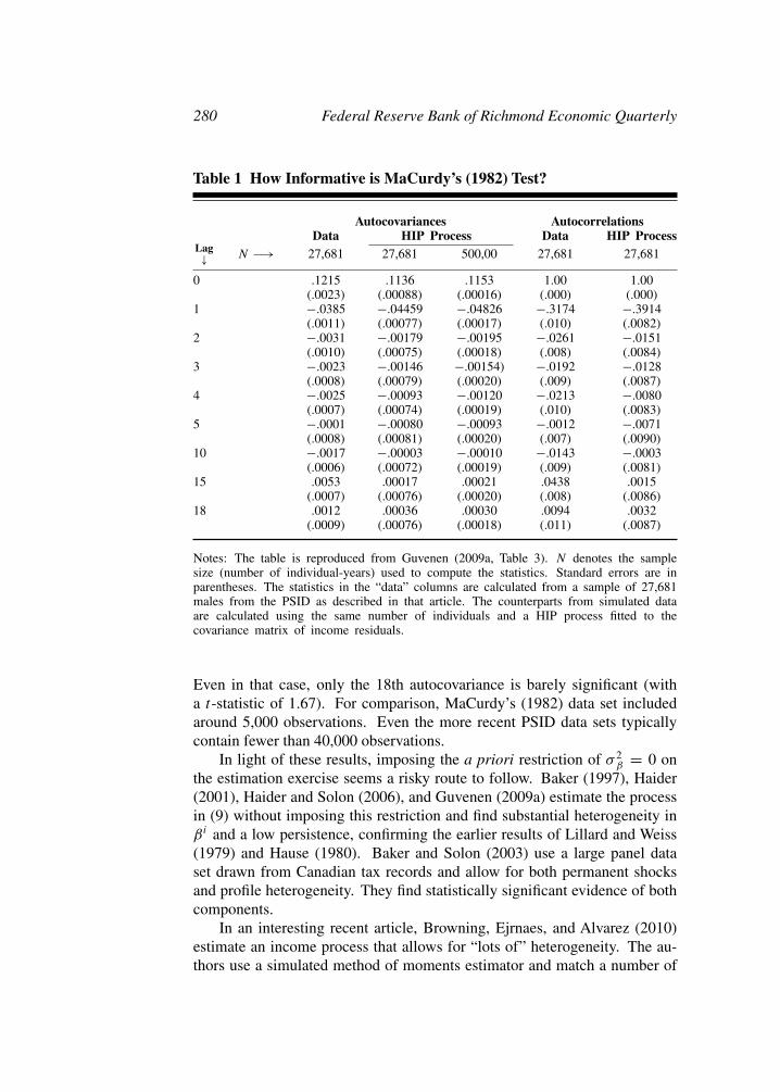
the second term to be negligible. He shows that for the value of persistence heestimates with the HIP process ($ -= 0.82), the autocovariances in (11) do noteven turn positive before the 13th lag (because the second term dominates),whereas MaCurdy only studies the first 5 lags. Second, he conducts a MonteCarlo analysis in which he simulates data using equation (9) with substantialheterogeneity in growth rates.28 The results of this analysis are reproducedhere in Table 1. MaCurdy’s test does not reject the false null hypothesis of& 24 = 0 for any sample size smaller than 500,000 observations (column 3)!
28 More concretely, the estimated value of & 24 used in his Monte Carlo analysis implies that
at age 55 more than 70 percent of wage inequality is because of profile heterogeneity.
280 Federal Reserve Bank of Richmond Economic Quarterly
Table 1 How Informative is MaCurdy’s (1982) Test?
Autocovariances AutocorrelationsData HIP Process Data HIP Process
Lag/ N &0 27,681 27,681 500,00 27,681 27,681
0 .1215 .1136 .1153 1.00 1.00(.0023) (.00088) (.00016) (.000) (.000)
1 &.0385 &.04459 &.04826 &.3174 &.3914(.0011) (.00077) (.00017) (.010) (.0082)
2 &.0031 &.00179 &.00195 &.0261 &.0151(.0010) (.00075) (.00018) (.008) (.0084)
3 &.0023 &.00146 &.00154) &.0192 &.0128(.0008) (.00079) (.00020) (.009) (.0087)
4 &.0025 &.00093 &.00120 &.0213 &.0080(.0007) (.00074) (.00019) (.010) (.0083)
5 &.0001 &.00080 &.00093 &.0012 &.0071(.0008) (.00081) (.00020) (.007) (.0090)
10 &.0017 &.00003 &.00010 &.0143 &.0003(.0006) (.00072) (.00019) (.009) (.0081)
15 .0053 .00017 .00021 .0438 .0015(.0007) (.00076) (.00020) (.008) (.0086)
18 .0012 .00036 .00030 .0094 .0032(.0009) (.00076) (.00018) (.011) (.0087)
Notes: The table is reproduced from Guvenen (2009a, Table 3). N denotes the samplesize (number of individual-years) used to compute the statistics. Standard errors are inparentheses. The statistics in the “data” columns are calculated from a sample of 27,681males from the PSID as described in that article. The counterparts from simulated dataare calculated using the same number of individuals and a HIP process fitted to thecovariance matrix of income residuals.
Even in that case, only the 18th autocovariance is barely significant (witha t-statistic of 1.67). For comparison, MaCurdy’s (1982) data set includedaround 5,000 observations. Even the more recent PSID data sets typicallycontain fewer than 40,000 observations.
In light of these results, imposing the a priori restriction of & 24 = 0 on
the estimation exercise seems a risky route to follow. Baker (1997), Haider(2001), Haider and Solon (2006), and Guvenen (2009a) estimate the processin (9) without imposing this restriction and find substantial heterogeneity in4 i and a low persistence, confirming the earlier results of Lillard and Weiss(1979) and Hause (1980). Baker and Solon (2003) use a large panel dataset drawn from Canadian tax records and allow for both permanent shocksand profile heterogeneity. They find statistically significant evidence of bothcomponents.
In an interesting recent article, Browning, Ejrnaes, and Alvarez (2010)estimate an income process that allows for “lots of” heterogeneity. The au-thors use a simulated method of moments estimator and match a number of

F. Guvenen: Macroeconomics with Heterogeneity 281
moments whose economic significance is more immediate than the covariancematrix of earnings residuals, which has typically been used as the basis of ageneralized method of moments estimation in the bulk of the extant literature.They uncover a lot of interesting heterogeneity, for example, in the innova-tion variance as well as in the persistence of AR(1) shocks. Moreover, they“find strong evidence against the hypothesis that any worker has a unit root.”Gustavsson and Osterholm (2010) use a long panel data set (1968–2005) fromadministrative wage records on Swedish individuals. They employ local-to-unity techniques on individual-specific time series and reject the unit rootassumption.
Inferring Risk versus Heterogeneity from Economic Choices
Finally, a number of recent articles examine the response of consumption toincome shocks to infer the nature of income risk. In an important article,Cunha, Heckman, and Navarro (2005) measure the fraction of individual-specific returns to education that are predictable by individuals by the timethey make their college decision versus the part that represents uncertainty.Assuming a complete markets structure, they find that slightly more than halfof the returns to education represent known heterogeneity from the perspectiveof individuals.
Guvenen and Smith (2009) study the joint dynamics of consumption andlabor income (using PSID data) in order to disentangle “known heterogeneity”from income risk (coming from shocks as well as from uncertainty regardingone’s own income growth rate). They conclude that a moderately persistentincome process ($ , 0.7–0.8) is consistent with the joint dynamics of incomeand consumption. Furthermore, they find that individuals have significantinformation about their own 4 i at the time they enter the labor market andhence face little uncertainty coming from this component. Overall, they con-clude that with income shocks of modest persistence and largely predictableincome growth rates, the income risk perceived by individuals is substan-tially smaller than what is typically assumed in calibrating incomplete marketsmodels (many of which borrow their parameter values from MaCurdy [1982],Abowd and Card [1989], and Meghir and Pistaferri [2004], among others).Along the same lines, Krueger and Perri (2009) use rich panel data on Italianhouseholds and conclude that the response of consumption to income suggestslow persistence for income shocks (or a high degree of partial insurance).29
Studying economic choices to disentangle risk from heterogeneity hasmany advantages. Perhaps most importantly, it allows researchers to bring a
29 A number of important articles have also studied the response of consumption to income,such as Blundell and Preston (1998) and Blundell, Pistaferri, and Preston (2008). These studies,however, assume the persistence of income shocks to be constant and instead focus on what canbe learned about the sizes of income shocks over time.

282 Federal Reserve Bank of Richmond Economic Quarterly
much broader set of data to bear on the question. For example, many dynamicchoices require individuals to carefully weigh the different future risks theyperceive against predictable changes before making a commitment. Decisionson home purchases, fertility, college attendance, retirement savings, and so onare all of this sort. At the same time, this line of research also faces importantchallenges: These analyses need to rely on a fully specified economic model,so the results can be sensitive to assumptions regarding the market structure,specification of preferences, and so on. Therefore, experimenting with differ-ent assumptions is essential before a definitive conclusion can be reached withthis approach. Overall, this represents a difficult but potentially very fruitfularea for future research.
Wealth, Health, and Other Shocks
One source of idiosyncratic risk that has received relatively little attentionuntil recently comes from shocks to wealth holdings, resulting for examplefrom fluctuations in housing prices and stock returns, among others. A largefraction of the fluctuations in housing prices are because of local or regionalfactors and are substantial (as the latest housing market crash showed onceagain). So these fluctuations can have profound effects on individuals’ eco-nomic choices. In one recent example, Krueger and Perri (2009) use paneldata on Italian households’ income, consumption, and wealth. They study theresponse of consumption to income and wealth shocks and find the latter tobe very important. Similarly, Mian and Sufi (2011) use individual-level datafrom 1997–2008 and show that housing price boom leads to significant equityextraction—about 25 cents for every dollar increase in prices—which in turnleads to higher leverage and personal default during this time. Their “con-servative” estimate is that home equity-based borrowing added $1.25 trillionin household debt and accounted for about 40 percent of new defaults from2006–2008.
Another source of idiosyncratic shocks is out-of-pocket medical expen-ditures (hospital bills, nursing home expenses, medications, etc.), which canpotentially have significant effects on household decisions. French and Jones(2004) estimate a stochastic process for health expenditures, modeled as anormal distribution adjusted to capture the risk of catastrophic health carecosts. Simulating this process, they show that 0.1 percent of households everyyear receive a health cost shock with a present value exceeding $125,000.Hubbard, Skinner, and Zeldes (1994, 1995) represent the earliest efforts to in-troduce such shocks into quantitative incomplete markets models. The 1995article shows that the interaction of such shocks with means-tested social in-surance programs is especially important to account for in order to understandthe very low savings rate of low-income individuals.
F. Guvenen: Macroeconomics with Heterogeneity 283
De Nardi, French, and Jones (2010) ask if the risk of large out-of-pocketmedical expenditures late in life can explain the savings behavior of the el-derly. They examine a new and rich data set called AHEAD, which is part ofthe Health and Retirement Survey conducted by the University of Michigan,which allows them to characterize medical expenditure risk for the elderly(even for those in their 90s) more precisely than previous studies, such asHubbard, Skinner, and Zeldes (1995) and Palumbo (1999).30 De Nardi,French, and Jones (2010) find out-of-pocket expenditures to rise dramaticallyat very old ages, which (in their estimated model) provides an explanationfor the lack of significant dissaving by the elderly. Ozkan (2010) shows thatthe life-cycle profile of medical costs (inclusive of the costs paid by privateand public insurers to providers) differs significantly between rich and poorhouseholds. In particular, on average, the medical expenses of the rich arehigher than those of the poor until mid-life, after which the expenses of thepoor exceed those of the rich—by 25 percent in absolute terms. Further, theexpenses of the poor have thick tails—lots of individuals with zero expensesand many with catastrophically high costs. He builds a model in which in-dividuals can invest in their health (i.e., preventive care), which affects thefuture distribution of health shocks and, consequently, the expected lifetime.High-income individuals do precisely this, which explains their higher spend-ing early on. Low-income individuals do the opposite, which ends up costingmore later in life. He concludes that a reform of the health care system thatencourages use of health care for low-income individuals has positive welfaregains, even when fully accounting for the increase in taxes required to pay forthem.
Endogenizing Credit Constraints
The basic Aiyagari model features a reduced-form specification for borrowingconstraints (8), and does not model the lenders’problem that gives rise to suchconstraints. As such, it is silent about potentially interesting variations inborrowing limits across individuals and states of the economy. A number ofrecent articles attempt to close this gap.
In one of the earliest studies of this kind, Athreya (2002) constructs ageneral equilibrium model of unsecured household borrowing to quantify thewelfare effects of the Bankruptcy Reform Act of 1999 in the United States. In
30 Palumbo’s estimates of medical expenditures are quite a bit smaller than those in De Nardi,French, and Jones (2010), which are largely responsible for the smaller effects he quantifies. DeNardi, French, and Jones (2010) argue that one reason for the discrepancy could be the fact thatPalumbo used data from the National Medical Care Expenditure Survey, which, unlike the AHEADdata set, does not contain direct measures of nursing home expenses. He did imputations from avariety of sources, which may be missing the large actual magnitude of such expenses found inthe AHEAD data set.

284 Federal Reserve Bank of Richmond Economic Quarterly
the pooling equilibrium of this model (which is what Athreya focuses on), thecompetitive lending sector charges a higher borrowing rate than the marketlending rate to break even (i.e., zero-profit condition), accounting for thefraction of households that will default. This framework allows him to studydifferent policies, such as changing the stringency of means testing as well aseliminating bankruptcy altogether.
In an important article, Chatterjee et al. (2007) build a model of personaldefault behavior and endogenous borrowing limits. The model features (i)several types of shocks—to earnings, preferences, and liabilities (e.g., hospi-tal and lawsuit bills, which precede a large fraction of defaults in the UnitedStates), (ii) a competitive banking sector, and (iii) post-bankruptcy legal treat-ment of defaulters that mimics the U.S. Chapter 7 bankruptcy code. The maincontribution of Chatterjee et al. (2007) is to show that a separating equi-librium exists in which banks offer a menu of debt contracts to householdswhose interest rates vary optimally with the level of borrowing to accountfor the changing default probability. Using a calibrated version of the model,they quantify the separate contributions of earnings, preferences, and liabilityshocks to debt and default. Chatterjee and Eyigungor (2011) introduce collat-eralized debt (i.e., mortgage debt) into this framework to examine the causesof the run-up in foreclosures and crash in housing prices after 2007.
Livshits, MacGee, and Tertilt (2007) study a model similar to Chatterjeeet al. (2007) in order to quantify the advantages to a “fresh start” bankruptcysystem (e.g., U.S. Chapter 7) against a European style system in which debtorscannot fully discharge their debt in bankruptcy. The key tradeoff is that dis-chargeable debts add insurance against bad shocks, helping to smooth acrossstates, but the inability to commit to future repayment increases interest ratesand limits the ability to smooth across time. Their model is quite similar toChatterjee et al. (2007), except that they model an explicit overlapping gener-ations structure. They calibrate the model to the age-specific bankruptcy rateand debt-to-earnings ratio. For their baseline parameterization, they find thatfresh-start bankruptcy is welfare improving, but that result is sensitive to theprocess for expenditure and income shocks, the shape of the earnings profile,and household size. Livshits, MacGee, and Tertilt (2010) build on this frame-work to evaluate several theories for the rise in personal bankruptcies since the1970s. Finally, Glover and Short (2010) use the model of personal bankruptcyto understand the incorporation of entrepreneurs. Incorporation protects theowners’ personal assets and their access to credit markets in case of default,but by increasing their likelihood of default, incorporation also implies a riskpremium is built into their borrowing rate.

F. Guvenen: Macroeconomics with Heterogeneity 285
From Bachelor(ette)s to Families
While the framework described above can shed light on some interesting dis-tributional issues (e.g., inequality in consumption, earnings, and wealth), it iscompletely silent on a crucial source of heterogeneity—the household struc-ture. In reality, individuals marry, divorce, have kids, and make their decisionsregarding consumption, savings, labor supply, and so on jointly with theseother life choices. For many economic and policy questions, the interactionbetween these domestic decisions and economic choices in an incompletemarkets world can have a first-order effect on the answers we get. Just togive a few examples, consider these facts: Men and women are well-known toexhibit different labor supply elasticities; the tax treatment of income variesdepending on whether an individual is single, married, and whether he/she haskids, etc.; the trends in the labor market participation rate in the United Statessince the 1960s have been markedly different for single and married women;the fractions of individuals who are married and divorced have changed sig-nificantly, again since the 1960s; and so on.
A burgeoning literature works to bring a richer household structure intomacroeconomics. For example, in an influential article, Greenwood,Seshadri, and Yorukoglu (2005) study the role of household technologies (thewidespread availability of washing machines, vacuum cleaners, refrigerators,etc.) in leading women into the labor market. Greenwood and Guner (2009)extend the analysis to study the marriage and divorce patterns since WorldWar II. Jones, Manuelli, and McGrattan (2003) explore the role of the closinggender wage gap for married women’s rising labor supply. Knowles (2007)argues that the working hours of men are too long when viewed through thelens of a unitary model of the household in which the average wage of femalesrises as in the data. He shows that introducing bargaining between spousesinto the model reconciles it with the data. Guner, Kaygusuz, and Ventura(2010) study the effects of potential reforms in the U.S. tax system in a modelof families with children and an extensive margin for female labor supply.Guvenen and Rendall (2011) study the insurance role of education for womenagainst divorce risk and the joint evolution of education trends with those inmarriage and divorce.
4. INEQUALITY IN CONSUMPTION, WEALTH,AND EARNINGS
A major use of heterogeneous-agent models is to study inequality or disper-sion in key economic outcomes, most notably in consumption, earnings, andwealth. The Aiyagari model—as well as its aggregate-shock augmented ver-sion, the Krusell-Smith model presented in the next section—takes earningsdispersion to be exogenous and makes predictions about inequality in con-sumption and wealth. The bulk of the incomplete markets literature follows
286 Federal Reserve Bank of Richmond Economic Quarterly
this lead in their analysis. Some studies introduce an endogenous labor supplychoice and instead specify the wage process to be exogenous, delivering earn-ings dispersion as an endogenous outcome (Pijoan-Mas [2006], Domeij andFloden [2006], Heathcote, Storesletten, and Violante [2008], among others).While this is a useful step forward, a lot of the dispersion in earnings beforeage 55 is because of wages and not hours, so the assumption of an exogenouswage process still leaves quite a bit to be understood. Other strands of theliterature attempt to close this gap by writing models that also generate wagedispersion as an endogenous outcome in the model—for example, because ofhuman capital accumulation (e.g., Guvenen and Kuruscu [2010, forthcoming],and Huggett, Ventura, and Yaron [2011]) or because of search frictions.31
Consumption Inequality
Two different dimensions of consumption inequality have received attentionin the literature. The first one concerns how much within-cohort consumptioninequality increases over the life cycle. The different views on this questionhave been summarized in Section 2.32 The second one concerns whether, andby how much, (overall) consumption inequality has risen in the United Statessince the 1970s, a question whose urgency was raised by the substantial risein wage inequality during the same time. In one of the earliest articles on thistopic, Cutler and Katz (1992) use data from the 1980s on U.S. householdsfrom the CE and find that the evolution of consumption inequality closelytracks the rise in wage inequality during the same time. This finding serves asa rejection of earlier claims in the literature (e.g., Jencks 1984) that the rise ofmeans-tested in-kind transfers starting in the 1970s had improved the materialwell-being of low-income households relative to what would be judged bytheir income statistics.
Interest in this question was reignited more recently by a thought-provokingarticle by Krueger and Perri (2006), who conclude from an analysis of CEdata that, from 1980–2003, within-group income inequality increased substan-tially more than within-group consumption inequality (in contrast, they find
31 The search literature is very large with many interesting models to cover. I do not discussthese models here because I cannot do justice to this extensive body of work in this limitedspace. For an excellent survey, see Rogerson, Shimer, and Wright (2005). Note, however, that asHornstein, Krusell, and Violante (2011) show, search models have trouble generating the magnitudesof wage dispersion we observe in the data.
32 Another recent article of interest is Aguiar and Hurst (2008), who examine the life-cyclemean and variance profiles of the subcomponents of consumption—housing, utility bills, clothing,food at home, food away from home, etc. They show rich patterns that vary across categories,whereby the variance rises monotonically for some categories, while being hump-shaped for others,and yet declining monotonically for some others. The same patterns are observed for the meanprofile. These disaggregated facts provide more food for thought to researchers.
F. Guvenen: Macroeconomics with Heterogeneity 287
that between-group income and consumption inequality tracked each other).33
They then propose an explanation based on the premise that the developmentof financial services in the U.S. economy has helped households smooth con-sumption fluctuations relative to income variation.
To investigate this story, they apply a model of endogenous debt constraintsas in Kehoe and Levine (1993). In this class of models, what is central isnot the ability of households to pay back their debt, but rather it is theirincentive or willingness to pay back. To give the right incentives, lenders canpunish a borrower that defaults, for example, by banning her from financialmarkets forever (autarky). However, if the individual borrows too much or ifautarky is not sufficiently costly, it may still make sense to default in certainstates of the world. Thus, given the parameters of the economic environment,lenders will compute the optimal state-contingent debt limit, which will ensurethat the borrower never defaults in equilibrium. Krueger and Perri (2006)notice that if income shocks are really volatile, then autarky is a really badoutcome, giving borrowers less incentive to default. Lenders who know this,in turn, are more willing to lend, which endogenously loosens the borrowingconstraints. This view of the last 30 years therefore holds that the rise in thevolatility of income shocks gave rise to the development of financial markets(more generous lending), which in turn led to a smaller rise in consumptioninequality.34
Heathcote, Storesletten, and Violante (2007) argue that the small rise inconsumption inequality can be explained simply if the rise in income shockshas been of a more transitory nature, since such shocks are easier to smooththrough self-insurance. Indeed, Blundell and Preston (1998) earlier madethe same observation and concluded that in the 1980s the rise in incomeshock variance was mostly permanent in nature (as evidenced by the observa-tion that income and consumption inequality grew together), whereas in the1990s it was mostly transitory given that the opposite was true. Heathcote,Storesletten, and Violante (2007) calibrate a fully specified model and showthat it can go a long way toward explaining the observed trends in consump-tion inequality. One point to keep in mind is that these articles take as giventhat the volatility of income shocks rose during this period, a conclusion thatis subject to uncertainty in light of the new evidence discussed above.
33 Attanasio, Battistin, and Ichimura (2007) question the use of the CE interview survey andargue that some expenditure items are poorly measured in the survey relative to another componentof CE, called the diary survey. They propose an optimal way of combining the two survey dataand find that consumption inequality, especially in the 1990s has increased more than what isrevealed by the interview survey alone.
34 Aguiar and Bils (2011) take a different approach and construct a measure of CE con-sumption by using data on income and (self-reported) savings rate by households. They argue thatconsumption inequality tracked income inequality closely in the past 30 years. Although this isstill preliminary work, the article raises some interesting challenges.
288 Federal Reserve Bank of Richmond Economic Quarterly
Before concluding, a word of caution about measurement. The appropri-ate price deflator for consumption may have trended differently for householdsin different parts of the income distribution (i.e., the “Walmart effect” at thelower end). To the extent that this effect is real, the measured trend in con-sumption inequality could be overstating the actual rise in the dispersion ofmaterial well-being. This issue still deserves a fuller exploration.
Wealth Inequality
The main question about wealth inequality is a cross-sectional one: Why dowe observe such enormous disparities in wealth, with a Gini coefficient ofabout 0.80 for net worth and a Gini exceeding 0.90 for financial wealth?
Economists have developed several models that can generate highlyskewed wealth distributions (see, for example, Huggett [1996], Krusell andSmith [1998], Quadrini [2000], Castaneda, Dıaz-Gimenez, and Rıos-Rull[2003], Guvenen [2006], and Cagetti and De Nardi [2006]). These modelstypically use one (or more) of three mechanisms to produce this inequality: (1)dispersion in luck in the form of large and persistent shocks to labor productiv-ity: the rich are luckier than the poor; (2) dispersion in patience or thriftiness:the rich save more than the poor; and (3) dispersion in rates of return: the richface higher asset returns than the poor. This subsection describes a baselinemodel and variations of it that incorporate various combinations of the threemain mechanisms that economists have used to generate substantial inequalityin general equilibrium models.35
Dispersion in Luck
Huggett (1996) asks how much progress can be made toward understandingwealth inequality using (i) a standard life-cycle model with (ii) Markovianidiosyncratic shocks, (iii) uncertain lifetimes, and (iv) a Social Security sys-tem. He finds that although the model can match the Gini coefficient forwealth in the United States, this comes from low-income households holdingtoo little wealth, rather than the extreme concentration of wealth at the topin the U.S. economy. Moreover, whereas in the U.S. data the dispersion ofwealth within each cohort is nearly as large as the dispersion across cohorts,the model understates the former significantly.
Castaneda, Dıaz-Gimenez, and Rıos-Rull (2003) study an enriched modelthat combines elements of Aiyagari (1994) and Huggett (1996). Specifically,the model (i) has a Social Security system, (ii) has perfectly altruistic bequests,
35 Some of the models discussed in this section contain aggregate shocks in addition toidiosyncratic ones. While aggregate shocks raise some technical issues that will be addressed inthe next section, they pose no problems for the exposition in this section.
F. Guvenen: Macroeconomics with Heterogeneity 289
(iii) allows for intergenerational correlation of earnings ability, (iv) has a pro-gressive labor and estate tax system as in the United States, and (v) allowsa labor supply decision. As for the stochastic process for earnings, they donot calibrate its properties based on microeconometric evidence on incomedynamics as is commonly done, but rather they choose its features (the 4 (4 transition matrix and four states of a Markov process) so that the modelmatches the cross-sectional distribution of earnings and wealth. To match theextreme concentration of wealth at the upper tail, this calibration procedureimplies that individuals must receive a large positive shock (about 1,060 timesthe median income level) with a small probability. This high income level isalso very fleeting—it lasts for about five years—which leads these high incomeindividuals to save substantially (for consumption smoothing) and results inhigh wealth inequality.
Dispersion in Patience
Laitner’s (1992, 2002) original insight was that wealth inequality could re-sult from a combination of: (1) random heterogeneity in lifetime incomesacross generations, and (2) altruistic bequests, which are constrained to benon-negative. Each newly born consumer in Laitner’s model receives a per-manent shock to his lifetime income and, unlike in the Aiyagari model, facesno further shocks to income during his lifetime. In essence, in Laitner’s modelonly households that earn higher than average lifetime income want to transfersome amount to their offspring, who are not likely to be as fortunate. Thisaltruistic motive makes these households effectively more thrifty (compared tothose that earn below average income) since they also care about future utility.Thus, even small differences in lifetime income can result in large differencesin savings rates—a fact empirically documented by Carroll (2000)—and hencein wealth accumulation.
The stochastic-beta model of Krusell and Smith (1998) is a variation onthis idea in a dynastic framework, where heterogeneity in thrift (i.e., in thetime-discount rate) is imposed exogenously.36 Being more parsimonious, thestochastic-beta model also allows for the introduction of aggregate shocks.Krusell and Smith show that even small differences in the time discount factorthat are sufficiently persistent are sufficient to generate the extreme skewnessof the U.S. wealth distribution. The intuition for this result will be discussedin a moment.
36 Notice that in this article I use # to denote the time discount factor and 4 was used todenote the income growth rate. I will continue with this convention, except when I specificallyrefer to the Krusell-Smith model, which has come to be known as a stochastic-beta model.

290 Federal Reserve Bank of Richmond Economic Quarterly
Dispersion in Rates of Return
Guvenen (2006) introduces return differentials into a standard stochastic grow-th model (i.e., in which consumers have identical, time-invariant discountfactors and idiosyncratic shocks do not exist). He allows all households totrade in a risk-free bond, but restricts one group of agents from accumulatingcapital. Quadrini (2000) and Cagetti and De Nardi (2006) study models ofinequality with entrepreneurs and workers, which can also generate skewedwealth distributions. The mechanisms have similar flavors: Agents who facehigher returns end up accumulating a substantial amount of wealth.
The basic mechanism in Guvenen (2006) can be described as follows.Nonstockholders have a precautionary demand for wealth (bonds), but theonly way they can save is if stockholders are willing to borrow. In con-trast, stockholders have access to capital accumulation, so they could smoothconsumption even if the bond market was completely shut down. Further-more, nonstockholders’ asset demand is even more inelastic because they areassumed to have a lower elasticity of intertemporal substitution (consistentwith empirical evidence) and therefore have a strong desire for consumptionsmoothing. Therefore, trading bonds for consumption smoothing is more im-portant for nonstockholders than it is for stockholders. As a result, stockhold-ers will only trade in the bond market if they can borrow at a low interest rate.This low interest rate in turn dampens nonstockholders’ demand for savingsfurther, and they end up with little wealth in equilibrium (and stockholders endup borrowing very little). Guvenen (2009b) shows that a calibrated version ofthis model easily generates the extremely skewed distribution of the relativewealth of stockholders to nonstockholders in the U.S. data.
Can We Tell Them Apart?
The determination of wealth inequality in the three models discussed so farcan be explained using variations of a diagram used by Aiyagari (1994). Theleft panel of Figure 2 shows how wealth inequality is determined in Laitner’smodel and, given their close relationship, in the Krusell-Smith model. Thetop solid curve originating from “&Bmin” plots the long-run asset demandschedule for the impatient agent; the bottom curve is for the patient agent. Awell-known feature of incomplete markets models is that the asset demandschedule is very flat for values of returns that are close to the time preferencerate, 0 (so # " 1/(1+0)). Thus, both types of individuals’ demand schedulesasymptote to their respective time preference rates (with 0patient < 0impatient).
37
If the equilibrium return (which must be lower than 0patient for an equilibriumto exist) is sufficiently close to 0patient, the high sensitivity of asset demands
37 See, for example, Aiyagari (1994) and references therein. This result also holds when assetreturns are stochastic (Chamberlain and Wilson 2000).
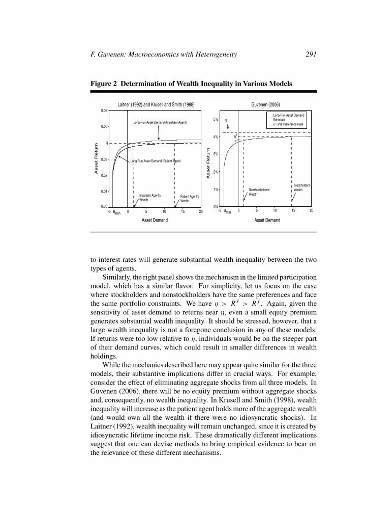
F. Guvenen: Macroeconomics with Heterogeneity 291
Figure 2 Determination of Wealth Inequality in Various Models
!
Asse
t R
etu
rn
Asse
t R
etu
rn
Asset Demand Asset Demand
Long-Run Asset Demand (Impatient Agent)
Long-Run Asset Demand (Patient Agent)
Impatient Agent'sWealth
Patient Agent'sWealth
Nonstockholders'Wealth
Stockholders'Wealth
Long-Run Asset Demand Schedule!: Time Preference Rate
Rs
Rf
-5 Bmin 0 5 10 15 20-5 Bmin 0 5 10 15 20
Laitner (1992) and Krusell and Smith (1998) Guvenen (2006)
0.00
0.01
0.02
0.03
R
0.05
0.06
0%
1%
2%
3%
4%
5%
to interest rates will generate substantial wealth inequality between the twotypes of agents.
Similarly, the right panel shows the mechanism in the limited participationmodel, which has a similar flavor. For simplicity, let us focus on the casewhere stockholders and nonstockholders have the same preferences and facethe same portfolio constraints. We have 0 > RS > Rf . Again, given thesensitivity of asset demand to returns near 0, even a small equity premiumgenerates substantial wealth inequality. It should be stressed, however, that alarge wealth inequality is not a foregone conclusion in any of these models.If returns were too low relative to 0, individuals would be on the steeper partof their demand curves, which could result in smaller differences in wealthholdings.
While the mechanics described here may appear quite similar for the threemodels, their substantive implications differ in crucial ways. For example,consider the effect of eliminating aggregate shocks from all three models. InGuvenen (2006), there will be no equity premium without aggregate shocksand, consequently, no wealth inequality. In Krusell and Smith (1998), wealthinequality will increase as the patient agent holds more of the aggregate wealth(and would own all the wealth if there were no idiosyncratic shocks). InLaitner (1992), wealth inequality will remain unchanged, since it is created byidiosyncratic lifetime income risk. These dramatically different implicationssuggest that one can devise methods to bring empirical evidence to bear onthe relevance of these different mechanisms.
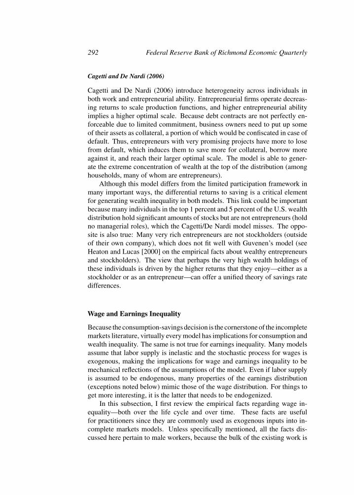
292 Federal Reserve Bank of Richmond Economic Quarterly
Cagetti and De Nardi (2006)
Cagetti and De Nardi (2006) introduce heterogeneity across individuals inboth work and entrepreneurial ability. Entrepreneurial firms operate decreas-ing returns to scale production functions, and higher entrepreneurial abilityimplies a higher optimal scale. Because debt contracts are not perfectly en-forceable due to limited commitment, business owners need to put up someof their assets as collateral, a portion of which would be confiscated in case ofdefault. Thus, entrepreneurs with very promising projects have more to losefrom default, which induces them to save more for collateral, borrow moreagainst it, and reach their larger optimal scale. The model is able to gener-ate the extreme concentration of wealth at the top of the distribution (amonghouseholds, many of whom are entrepreneurs).
Although this model differs from the limited participation framework inmany important ways, the differential returns to saving is a critical elementfor generating wealth inequality in both models. This link could be importantbecause many individuals in the top 1 percent and 5 percent of the U.S. wealthdistribution hold significant amounts of stocks but are not entrepreneurs (holdno managerial roles), which the Cagetti/De Nardi model misses. The oppo-site is also true: Many very rich entrepreneurs are not stockholders (outsideof their own company), which does not fit well with Guvenen’s model (seeHeaton and Lucas [2000] on the empirical facts about wealthy entrepreneursand stockholders). The view that perhaps the very high wealth holdings ofthese individuals is driven by the higher returns that they enjoy—either as astockholder or as an entrepreneur—can offer a unified theory of savings ratedifferences.
Wage and Earnings Inequality
Because the consumption-savings decision is the cornerstone of the incompletemarkets literature, virtually every model has implications for consumption andwealth inequality. The same is not true for earnings inequality. Many modelsassume that labor supply is inelastic and the stochastic process for wages isexogenous, making the implications for wage and earnings inequality to bemechanical reflections of the assumptions of the model. Even if labor supplyis assumed to be endogenous, many properties of the earnings distribution(exceptions noted below) mimic those of the wage distribution. For things toget more interesting, it is the latter that needs to be endogenized.
In this subsection, I first review the empirical facts regarding wage in-equality—both over the life cycle and over time. These facts are usefulfor practitioners since they are commonly used as exogenous inputs into in-complete markets models. Unless specifically mentioned, all the facts dis-cussed here pertain to male workers, because the bulk of the existing work is

F. Guvenen: Macroeconomics with Heterogeneity 293
available consistently for this group.38 Second, I discuss models that attemptto endogenize wages and explain the reported facts and trends.
Inequality Over the Life Cycle
The main facts about the evolution of (within-cohort) earnings inequality overthe life cycle were first documented by Deaton and Paxson (1994) and shownin the left panel of Figure 1. The same exercise has been repeated by numerousauthors using different data sets or time periods (among others, Storesletten,Telmer, and Yaron [2004a], Guvenen [2009a], Heathcote, Perri, and Violante[2010], and Kaplan [2010]). While the magnitudes differ somewhat, the basicfact that wage and earnings inequality rise substantially over the life cycle iswell-established.
One view is that this fact does not require an elaborate explanation, be-cause wages follow a very persistent, perhaps permanent, stochastic processas implied by the RIP model. Thus, the rising life-cycle inequality is simply areflection of the accumulation of such shocks, which drive up the variance oflog wages in a linear fashion (in the case of permanent shocks). I will continueto refer to this view as the RIP model because of its emphasis on persistent“shocks.”39
An alternative perspective, which has received attention more recently,emphasizes systematic factors—heterogeneity as opposed to random shocks.This view is essentially in the same spirit as the HIP model of the previous sec-tion. But it goes one step further by endogenizing the wage distribution basedon the human capital framework of Becker (1964) and Ben-Porath (1967),among others. In an influential article, Huggett, Ventura, and Yaron (2006)study the distributional implications of the standard Ben-Porath (1967) modelby asking about the types of heterogeneity that one needs to introduce to gen-erate patterns consistent with the U.S. data. They find that too much hetero-geneity in initial human capital levels results in the counterfactual implicationthat wage inequality should fall over the life cycle. In contrast, heterogene-ity in learning ability generates a rise in wage inequality consistent with thedata. A key implication of this finding is that the rise in wage inequality canbe generated without appealing to idiosyncratic shocks of any kind. Instead,it is the systematic fanning out of wage profiles, resulting from different in-vestment rates, that generates rising inequality over the life cycle. Guvenen,Kuruscu, and Ozkan (2009) and Huggett, Ventura, andYaron (2011) introduce
38 Some of the empirical trends discussed also apply to women, while others do not. SeeAutor, Katz, and Kearney (2008) for a comparative look at wage trends for males and femalesduring the period.
39 Of course, one can write deeper economic models that generate the observation that wagesfollow a random walk process, such as the learning model of Jovanovic (1979) in a search andmatching environment, or the optimal contracts in the limited commitment model of Harris andHolmstrom (1982).
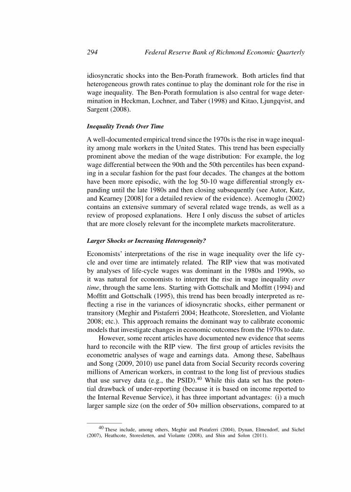
294 Federal Reserve Bank of Richmond Economic Quarterly
idiosyncratic shocks into the Ben-Porath framework. Both articles find thatheterogeneous growth rates continue to play the dominant role for the rise inwage inequality. The Ben-Porath formulation is also central for wage deter-mination in Heckman, Lochner, and Taber (1998) and Kitao, Ljungqvist, andSargent (2008).
Inequality Trends Over Time
A well-documented empirical trend since the 1970s is the rise in wage inequal-ity among male workers in the United States. This trend has been especiallyprominent above the median of the wage distribution: For example, the logwage differential between the 90th and the 50th percentiles has been expand-ing in a secular fashion for the past four decades. The changes at the bottomhave been more episodic, with the log 50-10 wage differential strongly ex-panding until the late 1980s and then closing subsequently (see Autor, Katz,and Kearney [2008] for a detailed review of the evidence). Acemoglu (2002)contains an extensive summary of several related wage trends, as well as areview of proposed explanations. Here I only discuss the subset of articlesthat are more closely relevant for the incomplete markets macroliterature.
Larger Shocks or Increasing Heterogeneity?
Economists’ interpretations of the rise in wage inequality over the life cy-cle and over time are intimately related. The RIP view that was motivatedby analyses of life-cycle wages was dominant in the 1980s and 1990s, soit was natural for economists to interpret the rise in wage inequality overtime, through the same lens. Starting with Gottschalk and Moffitt (1994) andMoffitt and Gottschalk (1995), this trend has been broadly interpreted as re-flecting a rise in the variances of idiosyncratic shocks, either permanent ortransitory (Meghir and Pistaferri 2004; Heathcote, Storesletten, and Violante2008; etc.). This approach remains the dominant way to calibrate economicmodels that investigate changes in economic outcomes from the 1970s to date.
However, some recent articles have documented new evidence that seemshard to reconcile with the RIP view. The first group of articles revisits theeconometric analyses of wage and earnings data. Among these, Sabelhausand Song (2009, 2010) use panel data from Social Security records coveringmillions of American workers, in contrast to the long list of previous studiesthat use survey data (e.g., the PSID).40 While this data set has the poten-tial drawback of under-reporting (because it is based on income reported tothe Internal Revenue Service), it has three important advantages: (i) a muchlarger sample size (on the order of 50+ million observations, compared to at
40 These include, among others, Meghir and Pistaferri (2004), Dynan, Elmendorf, and Sichel(2007), Heathcote, Storesletten, and Violante (2008), and Shin and Solon (2011).

F. Guvenen: Macroeconomics with Heterogeneity 295
most 50,000 in the PSID), (ii) no survey response error, and (iii) no attrition.Sabelhaus and Song find that the volatility of annual earnings growth in-creased during the 1970s, but that it declined monotonically during the 1980sand 1990s. Furthermore, applying the standard permanent-transitory decom-position as in Moffitt and Gottschalk (1995) and Meghir and Pistaferri (2004)reveals that permanent shock variances were stable and transitory shocks be-came smaller from 1980 into the 2000s. A separate study conducted by theCongressional Budget Office (2008), also using wage earnings from SocialSecurity records from 1980–2003, reached the same conclusion.41 Finally,Kopczuk, Saez, and Song (2010) document (also using Social Security data)that both long-run and short-run mobility have stayed remarkably stable fromthe 1960s into the 2000s. But this finding seems difficult to reconcile withMoffitt and Gottschalk (1995) and the subsequent literature that found perma-nent and transitory shock variances to have risen in different subperiods from1970 to the 2000s. If true, the latter would result in fluctuations in mobilitypatterns over these subperiods, which is not borne out in Kopczuk, Saez, andSong’s (2010) analysis.
Another piece of evidence from income data is offered by Haider (2001),who estimates a stochastic process for wages similar to the one in Moffittand Gottschalk (1995) and others, but with one key difference. He allowsfor individual-specific wage growth rates (HIP) and he also allows for thedispersion of growth rates to vary over time. The stochastic component isspecified as an ARMA(1,1). With this more flexible specification, he finds noevidence of a rise in the variance of income shocks after the 1970s, but insteadfinds a large increase in the dispersion of systematic wage growth rates.
A second strand of the literature studies the trends in labor market flowsin the United States. These articles do not find any evidence of rising jobinstability or churning, which one might expect to see in conjunction withlarger idiosyncratic shocks. In contrast, these studies document an across-the-board moderation in labor market flows. For example, Gottschalk andMoffitt (1999) focus on male workers between the ages of 20 and 62 andconclude their analysis as follows:
[W]e believe that a consistent picture is emerging on changes in jobstability and job security in the 1980s and 1990s. Job instability does
41 Sabelhaus-Song attribute the reason why some earlier studies found rising variances of wageshocks (e.g., Moffitt and Gottschalk 2008) to the inclusion of individuals with self-employmentincome and those who earn less than the Social Security minimum. Even though there are fewof these households, Sabelhaus and Song show that they make a big difference in the computedstatistics. Similarly, Shin and Solon (2011, 978–80) use PSID data and also do not find a trendin the volatility of wage earnings changes during the 1980s and 1990s. They argue that theincreasing volatility found in earlier studies, such as Dynan, Elmendorf, and Sichel (2007), seemsto be coming from the inclusion of some auxiliary types of income (from business, farming, etc.)whose treatment has been inconsistent in the PSID over the years.

296 Federal Reserve Bank of Richmond Economic Quarterly
not seem to have increased, and the consequences of separating from anemployer do not seem to have worsened.42
Shimer (2005, 2007) and Davis et al. (2010) extend this analysis to coverthe 2000s and use a variety of data sets to reach the same conclusion. Further,both articles show that expanding the sample of individuals to include womenand younger workers shows a declining trend in labor market flows and anincrease in job security.
Taking Stock
To summarize, the seeming consensus of the 1990s—that rising wage in-equality was driven by an increase in idiosyncratic shock variances—is beingchallenged by a variety of new evidence, some of which comes from data setsmany orders of magnitude larger than the surveys used in previous analyses.In addition, the evidence from labor market flows described above—while per-haps more indirect—raises questions about the sources of larger idiosyncraticshocks in a period where labor market transitions seem to have moderated.Although, it would be premature to conclude that the alternative view is thecorrect one—more evidence is needed to reach a definitive conclusion. Hav-ing said that, if this alternative view is true, and income shock variances havenot increased, this new “fact” would require economists to rethink a varietyof explanations put forward for various trends, which assumed a rise in shockvariances during this period.
5. HETEROGENEITY WITH AGGREGATE SHOCKS
Krusell and Smith (1998) add two elements to the basic Aiyagari framework.First, they introduce aggregate technology shocks. Second, they assume thatthe cumulative discount factor at time t (which was assumed to be #t be-fore), now follows the stochastic process #t = ##t&1, where # is a finite-stateMarkov chain. The stochastic evolution of the discount factors within a dy-nasty captures some elements of an explicit overlapping-generations structurewith altruism and less-than-perfect correlation in genes between parents andchildren, as in Laitner (1992). With this interpretation in mind, the evolutionof # is calibrated so that the average duration of any particular value of thediscount factor is equal to the lifetime of a generation. (Krusell and Smith[1997] study a version of this model where consumers are allowed to hold arisk-free bond in addition to capital.)
The specifics of the model are as follows. There are two types of shocks:(i) idiosyncratic employment status: (.e, .u) " (employed, unemployed);
42 They also say, “Almost all studies based on the various Current Population Surveys (CPS)supplements...show little change in the overall separation rates through the early 1990s.”

F. Guvenen: Macroeconomics with Heterogeneity 297
and (ii) aggregate productivity: (zg, zb) " (expansion, recession). Employ-ment status and aggregate productivity jointly evolve as a first-order Markovprocess. Assume that . is i.i.d. conditional on z, so the fraction of employedworkers (and hence l) only depends on z. Competitive markets imply
w (K, L, z) = (1 & ") z (K/L)&" , and r (K, L, z) = "z (K/L)"&1 . (12)
Finally, the entire wealth distribution, which I denote with5 is a state vari-able for this model, and let 5 = H(5, z; z ) denote its endogenous transitionfunction (or law of motion).
Krusell-Smith Algorithm
A key equilibrium object in this class of models is the law of motion, H . Inprinciple, computing this object is a formidable task since the distribution ofwealth is infinite-dimensional. Krusell and Smith (1997, 1998) show, however,that this class of models, when reasonably parameterized, exhibits “approxi-mate aggregation”: Loosely speaking, to predict future prices consumers needto forecast only a small set of statistics of the wealth distribution rather thanthe entire distribution itself. This result makes it possible to use numericalmethods to analyze this class of models. Another key feature of the Krusell-Smith algorithm is that it solves the model by simulating it. Specifically, thebasic version of the algorithm works as follows:
1. Approximate 5 with a finite number (I ) of moments. (H reduces to afunction mapping the I moments today into the I moments tomorrowdepending on z today.)
(a) We will start by selecting one moment—the mean—so I = 1.43
2. Select a family of functions for H . I will choose a log-linear functionfollowing Krusell and Smith.
V (k, .;5, z) = maxc,k
/U (c) + #E
/V#k, .; 5, z
$| z, .
00
c + k = w (K, L, z) ( l ( . + r (K, L, z) ( k, k * 0log K´ = a0 + a1 log K for z = zb
log K´ = b0 + b1 log K for z = zg
3. Make an (educated) initial guess about (a0, a1, b0, b1) =# yields initialguess for H0. Make also an initial guess for 50.
43 When we add more moments, we do not have to proceed as mean, variance, skewness,and so on. We can include, say, the wealth holdings of the top 10 percent of population, mean-to-median wealth ratio, etc.

298 Federal Reserve Bank of Richmond Economic Quarterly
4. Solve the consumer’s dynamic program. Using only the resulting de-cision rules, simulate
3kn,t
4N,T
n=1,t=1 for (N, T ) large.
5. Update H by estimating (where K = 1N
"Nn=1 kn):
log K´ = a0 + a1 log K for z = zb
log K´ = b0 + b1 log K for z = zg
6. Iterate on 4–5, until the R2 of this regression is “sufficiently high” andthe forecast variance is “small.”
(a) If accuracy remains insufficient, go back to step 1 and increase I .
Details
Educated Initial Guess
As with many numerical methods, a good initial guess is critical. More oftenthan not, the success or failure of a given algorithm will depend on the ini-tial guess. One idea (used by Krusell and Smith) is to first solve a standardrepresentative-agent real business cycle (RBC) model with the same param-eterization. Then estimate the coefficients (a0, a1, b0, b1) using capital seriessimulated from this model to obtain an initial guess for step 1 above.44 Moregenerally, a good initial guess can often be obtained by solving a simplifiedversion of the full model. Sometimes this simplification involves ignoringcertain constraints, sometimes by shutting down certain shocks, and so on.
Discretizing an AR(1) Process
Oftentimes, the exogenous driving force in incomplete markets models is as-sumed to be generated by anAR(1) process, which is discretized and convertedinto a Markov chain. One popular method for discretization is described inAiyagari (1993) and has been used extensively in the literature. However,an alternative method by Rouwenhorst (1995) (and which received far lessattention until recently) is far superior in the quality of the approximationthat it provides, especially when the process is very persistent, which is oftenthe case. Moreover, it is very easy to implement. Kopecky and Suen (2010)and Galindev and Lkhagvasuren (2010) provide comprehensive comparisonsof different discretization methods, which reveal the general superiority of
44 Can’t we update H without simulating? Yes, we can. Den Haan and Rendahl (2009)propose a method where they use the policy functions for capital holdings and integrate themover distribution +(k, .) of households across capital and employment status: K´ = Hj (K, z) =5
kj (k, .;5, z)d+(k, .). This works well when the decision rules are parameterized in a particularway. See den Haan and Rendahl (2009).
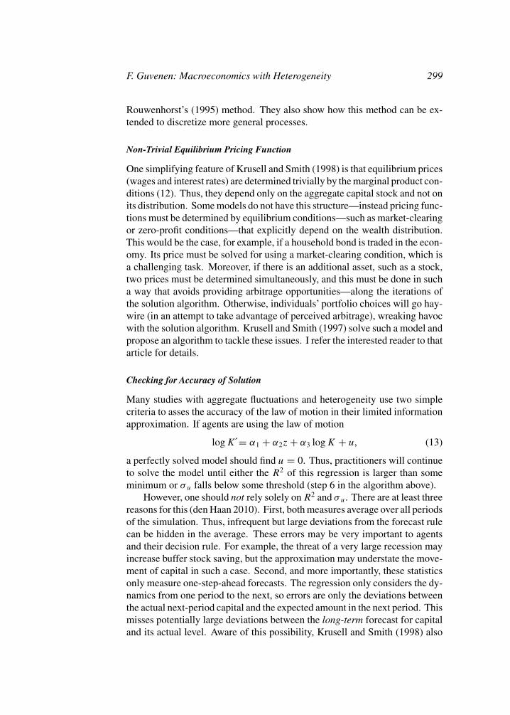
F. Guvenen: Macroeconomics with Heterogeneity 299
Rouwenhorst’s (1995) method. They also show how this method can be ex-tended to discretize more general processes.
Non-Trivial Equilibrium Pricing Function
One simplifying feature of Krusell and Smith (1998) is that equilibrium prices(wages and interest rates) are determined trivially by the marginal product con-ditions (12). Thus, they depend only on the aggregate capital stock and not onits distribution. Some models do not have this structure—instead pricing func-tions must be determined by equilibrium conditions—such as market-clearingor zero-profit conditions—that explicitly depend on the wealth distribution.This would be the case, for example, if a household bond is traded in the econ-omy. Its price must be solved for using a market-clearing condition, which isa challenging task. Moreover, if there is an additional asset, such as a stock,two prices must be determined simultaneously, and this must be done in sucha way that avoids providing arbitrage opportunities—along the iterations ofthe solution algorithm. Otherwise, individuals’ portfolio choices will go hay-wire (in an attempt to take advantage of perceived arbitrage), wreaking havocwith the solution algorithm. Krusell and Smith (1997) solve such a model andpropose an algorithm to tackle these issues. I refer the interested reader to thatarticle for details.
Checking for Accuracy of Solution
Many studies with aggregate fluctuations and heterogeneity use two simplecriteria to asses the accuracy of the law of motion in their limited informationapproximation. If agents are using the law of motion
log K´= "1 + "2z + "3 log K + u, (13)
a perfectly solved model should find u = 0. Thus, practitioners will continueto solve the model until either the R2 of this regression is larger than someminimum or & u falls below some threshold (step 6 in the algorithm above).
However, one should not rely solely on R2 and & u. There are at least threereasons for this (den Haan 2010). First, both measures average over all periodsof the simulation. Thus, infrequent but large deviations from the forecast rulecan be hidden in the average. These errors may be very important to agentsand their decision rule. For example, the threat of a very large recession mayincrease buffer stock saving, but the approximation may understate the move-ment of capital in such a case. Second, and more importantly, these statisticsonly measure one-step-ahead forecasts. The regression only considers the dy-namics from one period to the next, so errors are only the deviations betweenthe actual next-period capital and the expected amount in the next period. Thismisses potentially large deviations between the long-term forecast for capitaland its actual level. Aware of this possibility, Krusell and Smith (1998) also

300 Federal Reserve Bank of Richmond Economic Quarterly
check the R2 for forecasting prices 25 years ahead (100 model periods) andfind it to be extremely high as well! (They also check the maximum error inlong-term forecasts, which is very small.) Third, R2 is scaled by the left-handside of the regression. An alternative is to check the R2 of
log K´& log K = "1 + "2z + ("3 & 1) log K .
As a particularly dramatic demonstration, den Haan (2010) uses a savingsdecision rule that solves the Krusell and Smith (1998) model, simulates it forT periods, and estimates a law of motion in the form of equation (13). He thenmanipulates "1,"3 such that T &1" ut = 0 but the R2 falls from 0.9999 to0.999 and then 0.99. This has economically meaningful consequences: Thetime series standard deviation of the capital stock simulated from the perturbedversions of equation (13) falls to 70 percent and then 46 percent of the truefigure.
Finally, den Haan (2010) proposes a useful test that begins with the ap-proximated law of motion,
log K´= "1 + "2z + "3 log K + u, (14)
to generate a sequence of realizations of6Kt+1
7T
t=0and then compares these
to the sequence generated by aggregating from decision rules, the true law of
motion. Because6Kt+1
7T
t=0is obtained by repeatedly applying equation (14)
starting from K0, errors can accumulate. This is important because, in the truemodel, today’s choices depend on expectations about the future state, whichin turn depends on the future’s future expectations and so errors cascade. Tosystematically compare Kt to Kt , den Haan proposes an “essential accuracyplot.” For a sequence of shocks (not those originally used when estimating "to solve the model), generate a sequence of Kt and Kt . One can then comparemoments of the two simulated sequences. The “main focus” of the accuracytest is the errors calculated by ut =
888log Kt & log Kt
888, whose maximum shouldbe made close to zero.
Prices are More Sensitive than Quantities
The accuracy of the numerical solution becomes an even more critical issueif the main focus of analysis is (asset) prices rather than quantities. This isbecause prices are much more sensitive to approximation errors (see, e.g.,Christiano and Fisher [2000] and Judd and Guu [2001]). The results inChristiano and Fisher (2000) are especially striking. These authors comparea variety of different implementations of the “parameterized expectations”method and report the approximation errors resulting from each. For the stan-dard deviation of output, consumption, and investment (i.e., “quantities”), theapproximation errors range from less than 0.1 percent of the true value to 1
F. Guvenen: Macroeconomics with Heterogeneity 301
percent to 2 percent in some cases. For the stock and bond return and theequity premium, the errors regularly exceed 50 percent and are greater than100 percent in several cases. The bottom line is that the computation of assetprices requires extra care.
Pros and Cons
An important feature of the Krusell-Smith method is that it is a “local” solutionaround the stationary recursive equilibrium. In other words, this method relieson simulating a very long time series of data (e.g., capital series) and makingsure that after this path has converged to the ergodic set, the predictions ofagents are accurate for behavior inside that set. This has some advantagesand some disadvantages. One advantage is the efficiency gain compared tosolving a full recursive equilibrium, which enforces the equilibrium conditionsat every point of a somewhat arbitrary grid, regardless of whether or not a givenstate is ever visited in the stationary equilibrium.
One disadvantage is that if you take a larger deviation—say by setting K0
to a value well below the steady-state value—your “equilibrium functions”are likely to be inaccurate, and the behavior of the solution may differ sig-nificantly from the true solution. Why should we care about this? Supposeyou solve your model and then want to study a policy experiment where youeliminate taxes on savings. You would need to write a separate program fromthe “transition” between the two stationary equilibria. Instead, if you solvefor the full recursive equilibrium over a grid that contains both the initial andfinal steady states, you would not need to do this. However, solving for thefull equilibrium is often much harder and, therefore, is often overkill.
An Alternative to Krusell-Smith: Tracking History of Shocks
Some models have few exogenous state variables, but a large number of en-dogenous states. In such cases, using a formulation that keeps track of allthese state variables can make the numerical solution extremely costly or eveninfeasible. An alternative method begins with the straightforward observationthat all current endogenous state variables are nothing more than functionsof the infinite history of exogenous shocks. So, one could replace these en-dogenous states with the infinite history of exogenous states. Moreover, manymodels turn out to have “limited memory” in the sense that only the recenthistory of shocks matters in a quantitatively significant way, allowing us toonly track a truncated history of exogenous states. The first implementationof this idea I have been able to find is in Veracierto (1997), who studied amodel with plant-level investment irreversibilities, which give rise to S-s typepolicies. He showed that it is more practical to track a short history of the S-sthresholds instead of the current-period endogenous state variables.

302 Federal Reserve Bank of Richmond Economic Quarterly
As another example, consider an equilibrium model of the housing mar-ket where the only exogenous state is the interest rate, which evolves as aMarkov process. Depending on the precise model structure, the individualendogenous state variables can include the mortgage debt outstanding, thetime-to-maturity of the mortgage contract, etc., and the aggregate endogenousstate can include the entire distribution of agents over the individual states.This is potentially an enormously large state space! Arslan (2011) success-fully solves a model of this sort with realistic fixed-rate mortgage contracts,a life-cycle structure, and stochastic interest rates, using four lags of interestrates. Other recent examples that employ this basic approach include Chienand Lustig (2010), who solve an asset pricing model with aggregate and id-iosyncratic risk in which agents are subject to collateral constraints arisingfrom limited commitment, and Lorenzoni (2009), who solves a business cyclemodel with shocks to individuals’ expectations. In all these cases, tracking atruncated history turns out to provide computational advantages over choosingendogenous state variables that evolve in a Markovian fashion. One advantageof this approach is that it is often less costly to add an extra endogenous statevariable relative to the standard approach, because the same number of lagsmay still be sufficient. One drawback is that if the Markov process has manystates or the model has long memory, the method may not work as well.
6. WHEN DOES HETEROGENEITY MATTERFOR AGGREGATES?
As noted earlier, Krusell and Smith (1998) report that the time series behaviorof the aggregated incomplete markets model, by and large, looks very sim-ilar to the corresponding representative-agent model. A similar result wasreported in Rıos-Rull (1996). However, it is important to interpret these find-ings correctly and to not overgeneralize them. For example, even if a modelaggregates exactly, modeling heterogeneity can be very important for aggre-gate problems. This is because the problem solved by the representative agentcan look dramatically different from the problem solved by individuals (forexample, have very different preferences). Here, I discuss some importantproblems in macroeconomics where introducing heterogeneity yields conclu-sions quite different from a representative-agent model.
The Curse of Long Horizon
It is useful to start by discussing why incomplete markets do not matter in manymodels. Loosely speaking, this outcome follows from the fact that a long hori-zon makes individuals’ savings function approximately linear in wealth (i.e.,constant MPC out of wealth). As we saw in Section 1, the exact linearityof savings rule delivers exact demand aggregation in both Gorman (1961)

F. Guvenen: Macroeconomics with Heterogeneity 303
and Rubinstein’s (1974) theorems. As it turns out, even with idiosyncraticshocks, this near-linearity holds for wealth levels that are not immediately nearborrowing constraints. Thus, even though markets are incomplete, redistribut-ing wealth would matter little, and we have something that looks like demandaggregation!
Is there a way to get around this result? It is instructive to look at a con-crete example. Mankiw (1986) was one of the first articles in the literatureon the equity premium puzzle and one that gave prominence to the role ofheterogeneity. Mankiw (1986) shows that, in a two-period model with in-complete markets and idiosyncratic risk of the right form, one can generatean equity premium as large as desired. However, researchers who followedup on this promising lead (Telmer 1993, Heaton and Lucas 1996, and Kruselland Smith 1997) quickly came to a disappointing conclusion: Once agents inthese models are allowed to live for multiple periods, trading a single risk-freeasset yields sufficient consumption insurance, which in turn results in a tinyequity premium.
This result—that a sufficiently long horizon can dramatically weaken theeffects of incomplete markets—is quite general. In fact, Levine and Zame(2002) prove that if, in a single good economy with no aggregate shocks, (i)idiosyncratic income shocks follow a Markov process, (ii) marginal utility isconvex, and (iii) all agents have access to a single risk-free asset, then, asindividuals’ subjective time discount factor (#) approaches unity, incompletemarkets allocations (and utilities) converge to those from a complete marketseconomy with the same aggregate resources. Although Levine and Zame’sresult is theoretical for the limit of such economies (as # &0 1), it still soundsa cautionary note to researchers building incomplete markets models: Unlessshocks are extremely persistent and/or individuals are very impatient, thesemodels are unlikely to generate results much different from a representative-agent model.
Constantinides and Duffie (1996) show one way to get around the problemof a long horizon, which is also consistent with the message of Levine-Zame’stheorem. Essentially, they assume that individuals face permanent shocks,which eliminate the incentives to smooth such shocks. Therefore, they behaveas if they live in a static world and choose not to trade. Constantinides andDuffie also revive another feature of Mankiw’s (1986) model: Idiosyncraticshocks must have larger variance in recessions (i.e., countercyclical variances)to generate a large equity premium. With these two features, they show thatMankiw’s original insight can be made to work once again in an infinite horizonmodel. Storesletten, Telmer, and Yaron (2007) find that a calibrated modelalong the lines suggested by Constantinides and Duffie can generate about 1
4of the equity premium observed in the U.S. data.
The bottom line is that, loosely speaking, if incomplete markets matterin a model mainly through its effect on the consumption-saving decision, a
304 Federal Reserve Bank of Richmond Economic Quarterly
long horizon can significantly weaken the bite of incomplete markets. With along enough horizon, agents accumulate sufficient wealth and end up on thenearly linear portion of their savings function, delivering results not far froma complete markets model. This is also the upshot of Krusell and Smith’s(1998) analysis.
Examples Where Heterogeneity Does Matter
There are many examples in which heterogeneity does matter for aggregatephenomena. Here, I review some examples.
First, aggregating heterogeneous-agent models can give rise to preferencesfor the representative agent that may have nothing to do with the preferencesin the underlying model. A well-known example of such a transformation ispresent in the early works of Hansen (1985) and Rogerson (1988), who showthat in a model in which individuals have no intensive margin of labor sup-ply (i.e., zero Frisch labor supply elasticity), one can aggregate the model tofind that the representative agent has linear preferences in leisure (i.e., infiniteFrisch elasticity!). This conclusion challenges one of the early justificationsfor building models with microfoundations, which was to bring evidence frommicrodata to bear on the calibration of macroeconomic models. In an excel-lent survey article, Browning, Hansen, and Heckman (1999) issue an earlywarning, giving several examples where this approach is fraught with danger.
Building on the earlier insights of Hansen and Rogerson, Chang and Kim(2006) construct a model in which aggregate labor-supply elasticity dependson the reservation-wage distribution in the population. The economy is pop-ulated by households (husband and wife) that each supply labor only alongthe extensive margin: they either work full time or stay home. Workers arehit by idiosyncratic productivity shocks, causing them to move in and outof the labor market. The aggregate labor-supply elasticity of such an econ-omy is around one, greater than a typical microestimate and much greaterthan the Frisch elasticity one would measure at the intensive margin (whichis zero) in this model. The model thus provides a reconciliation between themicro- and macro-labor-supply elasticities. In a similar vein, Chang, Kim,and Schorfheide (2010) show that preference shifters that play an importantrole in discussions of aggregate policy are not invariant to policies if theyare generated from the aggregation of a heterogeneous-agent model. Such amodel also generates “wedges” at the aggregate level that do not translate intoany well-defined notion of preference shifters at the microlevel.45 Finally,Erosa, Fuster, and Kambourov (2009) build a life-cycle model of labor sup-ply, by combining and extending the ideas introduced in earlier articles, such
45 See Chari, Kehoe, and McGrattan (2007) for the definition of business-cycle wedges.

F. Guvenen: Macroeconomics with Heterogeneity 305
as Chang and Kim (2006) and Rogerson and Wallenius (2009). Their goalis to build a model with empirically plausible patterns of hours over the lifecycle and examine the response elasticities of labor supply to various policyexperiments.
In another context, Guvenen (2006) asks why macroeconomic modelsin the RBC tradition typically need to use a high elasticity of intertempo-ral substitution (EIS) to explain output and investment fluctuations, whereasEuler equation regressions (such as in Hall [1988] and Campbell and Mankiw[1990]) that use aggregate consumption data estimate a much smaller EIS(close to zero) to fit the data. He builds a model with two types of agentswho differ in their EIS. The model generates substantial wealth inequalityand much smaller consumption inequality, both in line with the U.S. data.Consequently, capital and investment fluctuations are mainly driven by therich (who hold almost all the wealth in the economy) and thus reflect the highEIS of this group. Consumption fluctuations, on the other hand, reflect anaverage that puts much more weight on the EIS of the poor, who contributesignificantly to aggregate consumption. Thus, a heterogeneous-agent modelis able to explain aggregate evidence that a single representative-agent modelhas trouble fitting.
In an asset pricing context, Constantinides and Duffie (1996), Chan andKogan (2002), and Guvenen (2011) show a similar result for risk aversion.Constantinides and Duffie (1996) show theoretically how the cross-sectionaldistribution of consumption in a heterogeneous-agent model gets translatedinto a higher risk aversion for the representative agent. Guvenen (2011) showsthat, in a calibrated model with limited stock market participation that matchesseveral asset pricing facts, the aggregate risk aversion is measured to be as highas 80, when the individuals’ risk aversion is only two. These results, as wellas the articles discussed above, confirm and amplify the concerns originallyhighlighted by Browning, Hansen, and Heckman (1999). The conclusion isthat researchers must be very careful when using microeconomic evidence tocalibrate representative-agent models.
7. COMPUTATION AND CALIBRATION
Because of their complexity, the overwhelming majority of models in thisliterature are solved on a computer using numerical methods.46 Thus, I nowturn to a discussion of computational issues that researchers often have toconfront when solving models with heterogeneity.
46 There are a few examples of analytical solutions and theoretical results established withheterogeneous-agent models. See, e.g., Constantinides and Duffie (1996), Heathcote, Storesletten,and Violante (2007), Rossi-Hansberg and Wright (2007), Wang (2009), and Guvenen and Kuruscu(forthcoming).
306 Federal Reserve Bank of Richmond Economic Quarterly
Calibration and Estimation: Avoid Local Search
Economists often need to minimize an objective function of multiple variablesthat has lots of kinks, jaggedness, and deep ridges. Consequently, the globalminimum is often surrounded by a large number of local minima. A typicalexample of such a problem arises when a researcher tries to calibrate severalstructural parameters of an economic model by matching some data moments.Algorithms based on local optimization methods (e.g., Newton-Raphson stylederivative-based methods or Nelder-Mead simplex style routines) very oftenget stuck in local minima because the objective surface is typically very rough(non-smooth).
It is useful to understand some of the sources of this roughness. For ex-ample, linear interpolation that is often used in approximating value functionsor decision rules generates an interpolated function that is non-differentiable(i.e., has kinks) at every knot point. Similarly, problems with (borrowing, port-folio, etc.) constraints can create significant kinks. Because researchers use afinite number of individuals to simulate data from the model (to compute mo-ments), a small change in the parameter value (during the minimization of theobjective) can move some individuals across the threshold—from being con-strained to unconstrained or vice versa—which can cause small jumps in theobjective value. And sometimes, the moments that the researcher decides tomatch would be inherently discontinuous in the underlying parameters (with afinite number of individuals), such as the median of a distribution (e.g., wealthholdings). Further compounding the problems, if the moments are not jointlysufficiently informative about the parameters to be calibrated, the objectivefunction would be flat in certain directions. As can be expected, trying tominimize a relatively flat function with lots of kinks, jaggedness, and evensmall jumps can be a very difficult task indeed.47
While the algorithm described here can be applied to the calibration ofany model, it is especially useful in models with heterogeneous agents—sincesuch models are time consuming to solve even once, an exhaustive search ofthe parameter space becomes prohibitively costly (which could be feasible insimpler models).
47 One simple, but sometimes overlooked, point is that when minimizing an objective functionof moments to calibrate a model, one should use the same “seeds” for the random elements ofthe model that are used to simulate the model in successive evaluations of the objective function.Otherwise, some of the change in objective value will be because of the inherent randomness indifferent draws of random variables. This can create significant problems with the minimizationprocedure.

F. Guvenen: Macroeconomics with Heterogeneity 307
A Simple Fully Parallelizable GlobalOptimization Algorithm
Here, I describe a global optimization algorithm that I regularly use for cal-ibrating models and I have found it to be very practical and powerful. It isrelatively straightforward to implement, yet allows full parallelization acrossany number of central processing unit (CPU) cores as well as across any num-ber of computers that are connected to the Internet. It requires no knowledgeof MPI, OpenMP, or related tools, and no knowledge of computer networkingother than using some commercially available synchronization tools (such asDropBox, SugarSync, etc.).
A broad outline of the algorithm is as follows. As with many global algo-rithms, this procedure combines a global stage with a local search stage thatis restarted at various locations in the parameter space. First, we would liketo search the parameter space as thoroughly as possible, but do so in as effi-cient a way as possible. Thoroughness is essential because we want to be surethat we found the true global minimum, so we are willing to sacrifice somespeed to ensure this. The algorithm proceeds by taking an initial starting point(chosen in a manner described momentarily) and conducting a local searchfrom that point on until the minimization routine converges as specified bysome tolerance. For local search, I typically rely on the Nelder-Mead’s down-hill simplex algorithm because it does not require derivative information (thatmay be inaccurate given the approximation errors in the model’s solution algo-rithm).48 The minimum function value as well as the parameter combinationthat attained that minimum are recorded in a file saved on the computer’s harddisk. The algorithm then picks the next “random” starting point and repeatsthe previous step of local minimization. The results are then added to theprevious file, which records all the local minima found up to that point.
Of course, the most obvious algorithm would be to keep doing a verylarge number of restarts of this sort and take the minimum of all the minimafound in the process. But this would be very time consuming and would not beparticularly efficient. Moreover, in many cases, the neighborhood of the globalminimum can feature many deep ridges and kinks nearby, which requires moreextensive searching near the global minimum, whereas the proposed approachwould devote more time to points far away from the true global minimum andto the points near it. Further, if the starting points are chosen literally randomly,this would also create potentially large efficiency losses, because these pointshave a non-negligible chance of falling near points previously tried. Becausethose areas have been previously searched, devoting more time is not optimal.
48 An alternative that can be much faster but requires a bit more tweaking for best perfor-mance is the trust region method of Zhang, Conn, and Scheinberg (2010) that builds on Powell’s(2009) BOBYQA algorithm.
308 Federal Reserve Bank of Richmond Economic Quarterly
A better approach is to use “quasi-random” numbers to generate the start-ing points. Quasi-random numbers (also called low-discrepancy sequences)are sequences of deterministic numbers that spread to any space in the maxi-mally separated way. They avoid the pitfall of random draws that may end upbeing too close to each other. Each draw in the sequence “knows” the locationof previous points drawn and attempts to fill the gaps as evenly as possible.49
Among a variety of sequences proposed in the literature, the Sobol’sequence isgenerally viewed to be superior in most practical applications, having a veryuniform filling of the space (i.e., maximally separated) even when a smallnumber of points is drawn, as well as a very fast algorithm that generates thesequence.50
Next, how do we use the accumulated information from previous restarts?As suggested by genetic algorithm heuristics, I combine information fromprevious best runs to adaptively direct the new restarts to areas that appearmore promising. This is explained further below. Now for the specifics of thealgorithm.
Algorithm 1 Let p be a J -dimensional parameter vector with generic elementpj , j = 1, ..., J.
• Step 0. Initialization:
– Determine bounds for each parameter, outside of which the objec-tive function should be set to a high value.
– Generate a sequence of Sobol’ numbers with a sequence length ofImax (the maximum anticipated number of restarts in the globalstage). Set the global iteration number i = 1.
• Step 1. Global Stage:
– Draw the ith (vector) value in the Sobol’ sequence: si .
– If i > 1, open and read from the text file “saved parameters.dat”the function values (and corresponding parameter vectors) of pre-viously found local minima. Denote the lowest function value foundas of iteration i&1 as f low
i&1 and the corresponding parameter vectoras plow
i&1.
– Generate a starting point for the local stage as follows:
49 Another common application of low-discrepancy sequences is in quasi-Monte Carlo inte-gration, where they have been found to improve time-to-accuracy by several orders of magnitude.
50 In a wide range of optimization problems, Kucherenko and Sytsko (2005) and Liberti andKucherenko (2005) find that Sobol’ sequences outperform Holton sequences, both in terms of com-putation time and probability of finding the global optimum. The Holton sequence is particularlyweak in high dimensional applications.

F. Guvenen: Macroeconomics with Heterogeneity 309
+ If i < Imin(< Imax), then use si as the initial guess: Si =si .Here, Imin is the threshold below which we use fully quasi-random starting points in the global stage.
+ If i * Imin, take the initial guess to be a convex combination ofsi and the parameter value that generated the best local minimaso far: Si = (1 & ) i)si + )plow
i&1. The parameter ) i ! [0, ) ]with ) < 1, and increases with i. For example, I found thata convex increasing function, such as ) i = min[) , (i/Imax)
2],works well in some applications. An alternative heuristic isgiven later.
+ As ) i is increased, local searches are restarted from a nar-rower part of the parameter space that yielded the lowest localminima before.
• Step 2: Local Stage:
– Using Si as a starting point, use the downhill simplex algorithm tosearch for a local minimum. (For the other vertices of the simplex,randomly draw starting points within the bounds of the parameterspace.)
– Stop when either (i) a certain tolerance has been achieved, (ii)function values do not improve more than a certain amount, or (iii)the maximum iteration number is reached.
– Open saved parameters.dat and record the local minimum found(function value and parameters).
• Step 3. Stopping Rule:
– Stop if the termination criterion described below is satisfied. If notgo to Step 1.
Termination Criterion
One useful heuristic criterion relies on a Bayesian procedure that estimates theprobability that the next local search will find a new local minimum based onthe rate at which new local minima have been located in past searches. Moreconcretely, if W different local minima have been found after K local searchesstarted from a set of uniformly distributed points, then the expectation of thenumber of local minima is
Wexp = W (K & 1) / (K & W & 2) ,
provided that K > W + 2. The searching procedure is terminated if Wexp <W +0.5. The idea is that, after a while of searching, if subsequent restarts keep
310 Federal Reserve Bank of Richmond Economic Quarterly
finding one of the same local minima found before, the chances of improve-ment in subsequent searches is not worth the additional time cost. Althoughthis is generally viewed as one of the most reliable heuristics, care must beapplied as with any heuristic.
Notice also that Wexp can be used to adaptively increase the value of ) i
in the global stage (Step 1 [3] above). The idea is that, as subsequent globalrestarts do not yield a new local minimum with a high enough probability,it is time to narrow the search and further explore areas of promising localminima. Because jaggedness and deep ridges cause local search methods tooften get stuck, we want to explore promising areas more thoroughly.
One can improve on this basic algorithm in various ways. I am going tomention a few that seem worth exploring.
Refinements: Clustering and Pre-Testing
First, suppose that in iteration k, the proposed starting point Sk ends up being“close” to one of the previous minima, say plow
n , for n < k. Then it is likelythat the search starting from Sk will end up converging to plow
n . But thenwe have wasted an entire cycle of local search without gaining anything. Toprevent this, one heuristic (called “clustering methods”) proceeds by defininga “region of attraction” (which is essentially a J -dimensional ball centered)around each one of the local minima found so far.51 Then the algorithm woulddiscard a proposed restarting point if it falls into the region attraction of anyprevious local minima. Because the local minimization stage is the mostcomputationally intensive step, this refinement of restarting the local searchonly once in a given region of attraction can result in significant computationalgains. Extensive surveys of clustering methods can be found in Rinnooy Kanand Timmer (1987a, 1987b).
Second, one can add a “pre-test” stage where N points from the Sobol’sequence are evaluated before any local search (i.e., in Step 0 above), and onlya subset of N+ < N points with lowest objective values are used as seeds inthe local search. The remaining points, as well as regions of attraction aroundthem are ignored as not promising. Notice that while this stage can improvespeed, it trades off reliability in the process.
Narrowing Down the Search Area
The file saved parameters.dat contains a lot of useful information gath-ered in each iteration to the global stage, which can be used more efficientlyas follows. As noted, the Nelder-Mead algorithm requires J + 1 candidate
51 While different formulas have been proposed for determining the optimal radius, theseformulas contain some undetermined coefficients, making the formulas less than useful in real lifeapplications.

F. Guvenen: Macroeconomics with Heterogeneity 311
points as inputs (the vertices of the J -dimensional simplex). One of thesepoints is given by Si , chosen as described above; the other vertices weredrawn randomly. But as we accumulate more information with every iterationon the global stage, if we keep finding local minima that seem to concentratein certain regions, it makes sense to narrow the range of values from whichwe pick the vertices. One way to do this is as follows: After a sufficientlylarge number of restarts have been completed, rank all the function valuesand take the lowest x percent of values (e.g., 10 percent or 20 percent). Thenfor each dimension, pick the minimum (pj
min) and maximum parameter value(pj
max) within this set of minima. Then, to generate vertices, take randomlysampled points between p
jmin and p
jmax in each dimension j . This allows
the simplex algorithm to search more intensively in a narrower area, whichcan improve results very quickly when there are ridges or jaggedness in theobjective function that make the algorithm get stuck.
Parallelizing the Algorithm
The algorithm can be parallelized in a relatively straightforward manner.52 Thebasic idea is to let each CPU core perform a separate local search in a differentpart of the parameter space, which is a time-consuming process. If we can domany such searches simultaneously, we can speed up the solution dramatically.One factor that makes parallelization simple is the fact that the CPU cores donot need to communicate with each other during the local search stage. Inbetween the local stages, each CPU core will contribute its findings (the lastlocal minimum it found along with the corresponding parameter vector) tothe collective wisdom recorded in saved parameters.dat and also get thelatest updated information about the best local minimum found so far fromthe same file. Thus, as long as all CPU cores have access to the same copy ofthe file saved parameters.dat, parallelization requires no more than a fewlines for housekeeping across CPUs. Here are some more specifics.
Suppose that we have a workstation with N CPU cores (for example,N = 4, 6, or 12). The first modification we need to make is to change theprogram to distinguish between the different “copies” of the code, running ondifferent CPU cores. This can be done by simply having the program ask theuser (only once, upon starting the code) to input an integer value, n, between1 and N , which uniquely identifies the “sequence number” of the particularinstance of the program running. Then open N terminal windows and launcha copy of the program in each window. Then for each one, enter a uniquesequence number n = 1, 2, ..., N .
52 I am assuming here that a compiled language, such as Fortran or C, is used to write theprogram. So multiple parallel copies of the same code can be run in different terminal windows.
312 Federal Reserve Bank of Richmond Economic Quarterly
Upon starting, each program will first simulate the same quasi-randomsequence regardless of n, but each run will pick a different element of thissequence as its own seed. For simplicity, suppose run n chooses the nthelement of the sequence as its seed and launches a local search from that point.After completion, each run will open the same file saved parameters.datand record the local minimum and parameter value it finds.53
Now suppose that all copies of the program complete their respective firstlocal searches, so there are N lines, each written by a different CPU core, inthe file saved parameters.dat. Then each run will start its second iterationand pick as its next seed the (N +n)th element of the quasi-random sequence.When the total number of iterations across all CPUs exceed some thresholdImin, then we would like to combine the quasi-random draw with the previousbest local minima as described in Step 1 (3) above. This is simple since allruns have access to the same copy of saved parameters.dat.54
Notice that this parallelization method is completely agnostic aboutwhether the CPU cores are on the same personal computer (PC) or dis-tributed across many PCs as long as all computers keep synchronized copies ofsaved parameters.dat. This can be achieved by using a synchronizationservice like DropBox. This feature easily allows one to harness the computa-tional power of many idle PCs distributed geographically with varying speedsand CPU cores.
8. FUTURE DIRECTIONS AND FURTHER READING
This article surveys the current state of the heterogeneous-agent models litera-ture and draws several conclusions. First, two key ingredients in such modelsare (i) the magnitudes and types of risk that the model builder feeds into themodel and (ii) the insurance opportunities allowed in the economy. In manycases, it is difficult, if not impossible, to measure each component separately.In other words, the assumptions a researcher makes regarding insurance op-portunities will typically affect the inference drawn about the magnitudes ofrisks and vice versa. Further complicating the problem is the measurement ofrisk: Individuals often have more information than the econometrician about
53 Because this opening and writing stage takes a fraction of a second, the likelihood thattwo or more programs access the file simultaneously and create a run-time error is negligible.
54 It is often useful for each run to keep track of the total number of local searches com-pleted by all CPUs—call this NLast . For example, sometimes the increase in ) i can be linkedto NLast . This number can be read as the total number of lines recorded up to that point insaved parameters.dat. Another use of this index is for determining which point in the sequenceto select as the next seed point. So as opposed to running n by selecting the (kN + n)th pointin the sequence where k is the number of local searches completed by run n, it could just pickthe (NLast + 1)th number in the sequence. This avoids leaving gaps in the sequence for seeds,in case some CPUs are much faster than others and hence finish many more local searches thanothers.

F. Guvenen: Macroeconomics with Heterogeneity 313
future changes in their lives. So, for example, a rise or fall in income that theeconometrician may view as a “shock” may in fact be partially or completelyanticipated by the individual. This suggests that equating income movementsobserved in the data with risk (as is often done in the literature) is likelyto overstate the true magnitude. This entanglement of “risk,” “anticipatedchanges,” and “insurance” presents a difficult challenge to researchers in thisarea. Although some recent progress has been made, more work remains.
A number of surveys contain very valuable material that are complemen-tary to this article. First, Heathcote, Storesletten, and Violante (2009) isa recent survey of quantitative macroeconomics with heterogeneous house-holds that is complementary to this article. Second, Browning, Hansen, andHeckman (1999) contains an extensive review of microeconomic models thatare often used as the foundations of heterogeneous-agent models. It high-lights several pitfalls in trying to calibrate macroeconomic models using mi-croevidence. Third, Meghir and Pistaferri (2011) provides a comprehensivetreatment of how earnings dynamics affect life-cycle consumption choice,which is closely related to the issues discussed in Section 3 of this survey.Finally, because heterogeneous-agent models use microeconomic survey datain increasingly sophisticated ways, a solid understanding of issues related tomeasurement error (which is pervasive in microdata) is essential. Failure to un-derstand such problems can wreak havoc with the empirical analysis. Bound,Brown, and Mathiowetz (2001) is an extensive and authoritative survey of thesubject.
The introduction of families into incomplete markets models representsan exciting area of current research. For many questions of empirical rele-vance, the interactions taking place within a household (implicit insurance,bargaining, etc.) can have first-order effects on how individuals respond toidiosyncratic changes. To give a few examples, Gallipoli and Turner (2011)document that the labor supply responses to disability shocks of single work-ers are larger and more persistent than those of married workers. They arguethat an important part of this difference has to do with the fact that couples areable to optimally change their time (and task) allocation within households inresponse to disability, an option not available to singles. This finding suggeststhat modeling households would be important for understanding the design ofdisability insurance policies. Similarly, Guner, Kaygusuz, and Ventura (2010)show that to quantify the effects of alternative tax reforms, it is important totake into account the joint nature of household labor supply. In fact, it is hardto imagine any distributional issue for which the household structure does notfigure in an important way.
Another promising area is the richer modeling of household finances in anera of ever-increasing sophistication in financial services. The Great Reces-sion, which was accompanied by a housing market crash and soaring personalbankruptcies, home foreclosures, and so on, has created a renewed sense of

314 Federal Reserve Bank of Richmond Economic Quarterly
urgency for understanding household balance sheets. Developments on twofronts—advances in theoretical modeling as discussed in Section 3, combinedwith richer data sources on credit histories and mortgages that are increasinglybecoming available to researchers—will make faster progress feasible in thisarea.
REFERENCES
Abowd, John M., and David E. Card. 1989. “On the Covariance Structure ofEarnings and Hours Changes.” Econometrica 57 (March): 411–45.
Acemoglu, Daron. 2002. “Technical Change, Inequality, and the LaborMarket.” Journal of Economic Literature 40 (March): 7–72.
Aguiar, Mark, and Erik Hurst. 2008. “Deconstructing LifecycleExpenditures.” Working Paper, University of Rochester.
Aguiar, Mark, and Mark Bils. 2011. “Has Consumption Inequality MirroredIncome Inequality?” Working Paper, University of Rochester.
Aiyagari, S. Rao. 1993. “Uninsured Idiosyncratic Risk and AggregateSaving.” Federal Reserve Bank of Minneapolis Working Paper 502.
Aiyagari, S. Rao. 1994. “Uninsured Idiosyncratic Risk and AggregateSaving.” The Quarterly Journal of Economics 109 (August): 659–84.
Altug, Sumru, and Robert A. Miller. 1990. “Household Choices inEquilibrium.” Econometrica 58 (May): 543–70.
Arslan, Yavuz. 2011. “Interest Rate Fluctuations and Equilibrium in theHousing Market.” Working Paper, Central Bank of the Republic ofTurkey.
Athreya, Kartik B. 2002. “Welfare Implications of the Bankruptcy ReformAct of 1999.” Journal of Monetary Economics 49 (November):1,567–95.
Attanasio, Orazio, and Steven J. Davis. 1996. “Relative Wage Movementsand the Distribution of Consumption.” Journal of Political Economy 104(December): 1,227–62.
Attanasio, Orazio, Erich Battistin, and Hidehiko Ichimura. 2007. “WhatReally Happened to Consumption Inequality in the United States?” InHard-to-Measure Goods and Services: Essays in Honour of ZviGriliches, edited by E. Berndt and C. Hulten. Chicago: University ofChicago Press.
F. Guvenen: Macroeconomics with Heterogeneity 315
Attanasio, Orazio P., James Banks, Costas Meghir, and Guglielmo Weber.1999. “Humps and Bumps in Lifetime Consumption.” Journal ofBusiness & Economic Statistics 17 (January): 22–35.
Autor, David H., Lawrence F. Katz, and Melissa S. Kearney. 2008. “Trendsin U.S. Wage Inequality: Revising the Revisionists.” The Review ofEconomics and Statistics 90 (2): 300–23.
Badel, Alejandro, and Mark Huggett. 2007. “Interpreting Life-CycleInequality Patterns as an Efficient Allocation: Mission Impossible?”Working Paper, Georgetown University.
Baker, Michael. 1997. “Growth-Rate Heterogeneity and the CovarianceStructure of Life-Cycle Earnings.” Journal of Labor Economics 15(April): 338–75.
Baker, Michael, and Gary Solon. 2003. “Earnings Dynamics and Inequalityamong Canadian Men, 1976–1992: Evidence from Longitudinal IncomeTax Records.” Journal of Labor Economics 21 (April): 267–88.
Becker, Gary S. 1964. Human Capital: A Theoretical and EmpiricalAnalysis, with Special Reference to Education. Chicago: University ofChicago Press.
Ben-Porath, Yoram. 1967. “The Production of Human Capital and the LifeCycle of Earnings.” Journal of Political Economy 75 (4): 352–65.
Bewley, Truman F. Undated. “Interest Bearing Money and the EquilibriumStock of Capital.” Working Paper.
Blundell, Richard, and Ian Preston. 1998. “Consumption Inequality AndIncome Uncertainty.” The Quarterly Journal of Economics 113 (May):603–40.
Blundell, Richard, Luigi Pistaferri, and Ian Preston. 2008. “ConsumptionInequality and Partial Insurance.” American Economic Review 98(December): 1,887–921.
Bound, John, Charles Brown, and Nancy Mathiowetz. 2001. “MeasurementError in Survey Data.” In Handbook of Econometrics, edited by J. J.Heckman and E. E. Leamer. Amsterdam: Elsevier; 3,705–843.
Browning, Martin, Lars Peter Hansen, and James J. Heckman. 1999. “MicroData and General Equilibrium Models.” In Handbook ofMacroeconomics, edited by J. B. Taylor and M. Woodford. Amsterdam:Elsevier; 543–633.
Browning, Martin, Mette Ejrnaes, and Javier Alvarez. 2010. “ModellingIncome Processes with Lots of Heterogeneity.” Review of EconomicStudies 77 (October): 1,353–81.
316 Federal Reserve Bank of Richmond Economic Quarterly
Cagetti, Marco, and Mariacristina De Nardi. 2006. “Entrepreneurship,Frictions, and Wealth.” Journal of Political Economy 114 (October):835–70.
Campbell, John Y., and N. Gregory Mankiw. 1990. “Consumption, Income,and Interest Rates: Reinterpreting the Time Series Evidence.” WorkingPaper 2924. Cambridge, Mass.: National Bureau of Economic Research(May).
Carroll, Christopher. 2000. “Why Do the Rich Save So Much?” In DoesAtlas Shrug? The Economic Consequences of Taxing the Rich, edited byJoel Slemrod. Boston: Harvard University Press, 466–84.
Carroll, Christopher D. 1991. “Buffer Stock Saving and the PermanentIncome Hypothesis.” Board of Governors of the Federal Reserve SystemWorking Paper Series/Economic Activity Section 114.
Carroll, Christopher D. 1997. “Buffer-Stock Saving and the LifeCycle/Permanent Income Hypothesis.” The Quarterly Journal ofEconomics 112 (February): 1–55.
Carroll, Christopher D., and Andrew A. Samwick. 1997. “The Nature ofPrecautionary Wealth.” Journal of Monetary Economics 40 (September):41–71.
Caselli, Francesco, and Jaume Ventura. 2000. “A Representative ConsumerTheory of Distribution.” American Economic Review 90 (September):909–26.
Castaneda, Ana, Javier Dıaz-Gimenez, and Jose-Vıctor Rıos-Rull. 2003.“Accounting for the U.S. Earnings and Wealth Inequality.” The Journalof Political Economy 111 (August): 818–57.
Chamberlain, Gary, and Charles A. Wilson. 2000. “Optimal IntertemporalConsumption Under Uncertainty.” Review of Economic Dynamics 3(July): 365–95.
Chan, Yeung Lewis, and Leonid Kogan. 2002. “Catching up with theJoneses: Heterogeneous Preferences and the Dynamics of Asset Prices.”Journal of Political Economy 110 (December): 1,255–85.
Chang, Yongsung, and Sun-Bin Kim. 2006. “From Individual to AggregateLabor Supply: A Quantitative Analysis based on a Heterogeneous-AgentMacroeconomy.” International Economic Review 47 (1): 1–27.
Chang, Yongsung, Sun-Bin Kim, and Frank Schorfheide. 2010. “LaborMarket Heterogeneity, Aggregation, and the Lucas Critique.” WorkingPaper 16401. Cambridge, Mass.: National Bureau of EconomicResearch.

F. Guvenen: Macroeconomics with Heterogeneity 317
Chari, V. V., Patrick J. Kehoe, and Ellen R. McGrattan. 2007. “BusinessCycle Accounting.” Econometrica 75 (3): 781–836.
Chatterjee, Satyajit, and Burcu Eyigungor. 2011. “A Quantitative Analysis ofthe U.S. Housing and Mortgage Markets and the Foreclosure Crisis.”Federal Reserve Bank of Philadelphia Working Paper 11-26 (July).
Chatterjee, Satyajit, Dean Corbae, Makoto Nakajima, and Jose-VıctorRıos-Rull. 2007. “A Quantitative Theory of Unsecured Consumer Creditwith Risk of Default.” Econometrica 75 (November): 1,525–89.
Chien, YiLi, and Hanno Lustig. 2010. “The Market Price of Aggregate Riskand the Wealth Distribution.” Review of Financial Studies 23 (April):1,596–650.
Christiano, Lawrence J., and Jonas D. M. Fisher. 2000. “Algorithms forSolving Dynamic Models with Occasionally Binding Constraints.”Journal of Economic Dynamics and Control 24 (July): 1,179–232.
Clarida, Richard H. 1987. “Consumption, Liquidity Constraints, and AssetAccumulation in the Presence of Random Income Fluctuations.”International Economic Review 28 (June): 339–51.
Clarida, Richard H. 1990. “International Lending and Borrowing in aStochastic, Stationary Equilibrium.” International Economic Review 31(August): 543–58.
Cochrane, John H. 1991. “A Simple Test of Consumption Insurance.”Journal of Political Economy 99 (October): 957–76.
Congressional Budget Office. 2008. “Recent Trends in the Variability ofIndividual Earnings and Family Income.” Washington, D.C.: CBO(June).
Constantinides, George M. 1982. “Intertemporal Asset Pricing withHeterogeneous Consumers and Without Demand Aggregation.” Journalof Business 55 (April): 253–67.
Constantinides, George M., and Darrell Duffie. 1996. “Asset Pricing withHeterogeneous Consumers.” Journal of Political Economy 104 (April):219–40.
Cunha, Flavio, James Heckman, and Salvador Navarro. 2005. “SeparatingUncertainty from Heterogeneity in Life Cycle Earnings.” OxfordEconomic Papers 57 (2): 191–261.
Cutler, David M., and Lawrence F. Katz. 1992. “Rising Inequality? Changesin the Distribution of Income and Consumption in the 1980’s.” AmericanEconomic Review 82 (May): 546–51.
318 Federal Reserve Bank of Richmond Economic Quarterly
Davis, Steven J., R. Jason Faberman, John Haltiwanger, Ron Jarmin, andJavier Miranda. 2010. “Business Volatility, Job Destruction, andUnemployment.” Working Paper 14300. Cambridge, Mass.: NationalBureau of Economic Research (September).
De Nardi, Mariacristina, Eric French, and John B. Jones. 2010. “Why Do theElderly Save? The Role of Medical Expenses.” Journal of PoliticalEconomy 118 (1): 39–75.
Deaton, Angus. 1991. “Saving and Liquidity Constraints.” Econometrica 59(September): 1,221–48.
Deaton, Angus, and Christina Paxson. 1994. “Intertemporal Choice andInequality.” Journal of Political Economy 102 (June): 437–67.
Debreu, Gerard. 1959. Theory of Value. New York: John Wiley and Sons.
den Haan, Wouter J. 2010. “Assessing the Accuracy of the Aggregate Law ofMotion in Models with Heterogeneous Agents.” Journal of EconomicDynamics and Control 34 (January): 79–99.
den Haan, Wouter J., and Pontus Rendahl. 2009. “Solving the IncompleteMarkets Model with Aggregate Uncertainty Using ExplicitAggregation.” Working Paper, University of Amsterdam.
Domeij, David, and Martin Floden. 2006. “The Labor-Supply Elasticity andBorrowing Constraints: Why Estimates are Biased.” Review ofEconomic Dynamics 9 (April): 242–62.
Dynan, Karen E., Douglas W. Elmendorf, and Daniel E. Sichel. 2007. “TheEvolution of Household Income Volatility.” Federal Reserve BoardWorking Paper 2007-61.
Erosa, Andres, Luisa Fuster, and Gueorgui Kambourov. 2009. “TheHeterogeneity and Dynamics of Individual Labor Supply over the LifeCycle: Facts and Theory.” Working Paper, University of Toronto.
Flavin, Marjorie A. 1981. “The Adjustment of Consumption to ChangingExpectations About Future Income.” Journal of Political Economy 89(October): 974–1,009.
French, Eric, and John Bailey Jones. 2004. “On the Distribution andDynamics of Health Care Costs.” Journal of Applied Econometrics 19(6): 705–21.
Galindev, Ragchaasuren, and Damba Lkhagvasuren. 2010. “Discretization ofHighly Persistent Correlated AR(1) Shocks.” Journal of EconomicDynamics and Control 34 (July): 1,260–76.
Gallipoli, Giovanni, and Laura Turner. 2011. “Household Responses toIndividual Shocks: Disability and Labour Supply.” Working Paper,University of British Columbia.

F. Guvenen: Macroeconomics with Heterogeneity 319
Glover, Andrew, and Jacob Short. 2010. “Bankruptcy, Incorporation, and theNature of Entrepreneurial Risk.” Working Paper, University of WesternOntario.
Gorman, William M. 1961. “On a Class of Preference Fields.”Metroeconomica 13 (June): 53–6.
Gottschalk, Peter, and Robert Moffitt. 1994. “The Growth of EarningsInstability in the U.S. Labor Market.” Brookings Papers on EconomicActivity 25 (2): 217–72.
Gottschalk, Peter, and Robert Moffitt. 1999. “Changes in Job Instability andInsecurity Using Monthly Survey Data.” Journal of Labor Economics 17(October): S91–126.
Gourinchas, Pierre-Olivier, and Jonathan A. Parker. 2002. “Consumptionover the Life Cycle.” Econometrica 70 (January): 47–89.
Greenwood, Jeremy, Ananth Seshadri, and Mehmet Yorukoglu. 2005.“Engines of Liberation.” Review of Economic Studies 72 (1): 109–33.
Greenwood, Jeremy, and Nezih Guner. 2009. “Marriage and Divorce sinceWorld War II: Analyzing the Role of Technological Progress on theFormation of Households.” In NBER Macroeconomics Annual, Vol. 23.Cambridge, Mass.: National Bureau of Economic Research, 231–76.
Guner, Nezih, Remzi Kaygusuz, and Gustavo Ventura. 2010. “Taxation andHousehold Labor Supply.” Working Paper, Arizona State University.
Gustavsson, Magnus, and Par Osterholm. 2010. “Does the Labor-IncomeProcess Contain a Unit Root? Evidence from Individual-Specific TimeSeries.” Working Paper, Uppsala University.
Guvenen, Fatih. 2006. “Reconciling Conflicting Evidence on the Elasticityof Intertemporal Substitution: A Macroeconomic Perspective.” Journalof Monetary Economics 53 (October): 1,451–72.
Guvenen, Fatih. 2007a. “Do Stockholders Share Risk More Effectively thanNonstockholders?” The Review of Economics and Statistics 89 (2):275–88.
Guvenen, Fatih. 2007b. “Learning Your Earning: Are Labor Income ShocksReally Very Persistent?” American Economic Review 97 (June):687–712.
Guvenen, Fatih. 2009a. “An Empirical Investigation of Labor IncomeProcesses.” Review of Economic Dynamics 12 (January): 58–79.
Guvenen, Fatih. 2009b. “A Parsimonious Macroeconomic Model for AssetPricing.” Econometrica 77 (November): 1,711–50.
Guvenen, Fatih. 2011. “Limited Stock Market Participation Versus ExternalHabit: An Intimate Link.” University of Minnesota Working Paper 450.
320 Federal Reserve Bank of Richmond Economic Quarterly
Guvenen, Fatih, and Anthony A. Smith. 2009. “Inferring Labor Income Riskfrom Economic Choices: An Indirect Inference Approach.” WorkingPaper, University of Minnesota.
Guvenen, Fatih, and Burhanettin Kuruscu. 2010. “A Quantitative Analysis ofthe Evolution of the U.S. Wage Distribution, 1970–2000.” In NBERMacroeconomics Annual 2009 24 (1): 227–76.
Guvenen, Fatih, and Burhanettin Kuruscu. Forthcoming. “Understanding theEvolution of the U.S. Wage Distribution: A Theoretical Analysis.”Journal of the European Economic Association.
Guvenen, Fatih, and Michelle Rendall. 2011. “Emancipation ThroughEducation.” Working Paper, University of Minnesota.
Guvenen, Fatih, Burhanettin Kuruscu, and Serdar Ozkan. 2009. “Taxation ofHuman Capital and Wage Inequality: A Cross-Country Analysis.”Working Paper 15526. Cambridge, Mass.: National Bureau of EconomicResearch (November).
Haider, Steven J. 2001. “Earnings Instability and Earnings Inequality ofMales in the United States: 1967–1991.” Journal of Labor Economics19 (October): 799–836.
Haider, Steven, and Gary Solon. 2006. “Life-Cycle Variation in theAssociation between Current and Lifetime Earnings.” AmericanEconomic Review 96 (September): 1,308–20.
Hall, Robert E. 1988. “Intertemporal Substitution in Consumption.” Journalof Political Economy 96 (April): 339–57.
Hall, Robert E., and Frederic S. Mishkin. 1982. “The Sensitivity ofConsumption to Transitory Income: Estimates from Panel Data onHouseholds.” Econometrica 50 (March): 461–81.
Hansen, Gary D. 1985. “Indivisible Labor and the Business Cycle.” Journalof Monetary Economics 16 (November): 309–27.
Harris, Milton, and Bengt Holmstrom. 1982. “A Theory of Wage Dynamics.”Review of Economic Studies 49 (July): 315–33.
Hause, John C. 1980. “The Fine Structure of Earnings and the On-the-JobTraining Hypothesis.” Econometrica 48 (May): 1,013–29.
Hayashi, Fumio, Joseph Altonji, and Laurence Kotlikoff. 1996.“Risk-Sharing between and within Families.” Econometrica 64 (March):261–94.
Heathcote, Jonathan, Fabrizio Perri, and Giovanni L. Violante. 2010.“Unequal We Stand: An Empirical Analysis of Economic Inequality inthe United States, 1967–2006.” Review of Economic Dynamics 13(January): 15–51.
F. Guvenen: Macroeconomics with Heterogeneity 321
Heathcote, Jonathan, Kjetil Storesletten, and Giovanni L. Violante. 2007.“Consumption and Labour Supply with Partial Insurance: An AnalyticalFramework.” CEPR Discussion Papers 6280 (May).
Heathcote, Jonathan, Kjetil Storesletten, and Giovanni L. Violante. 2008.“The Macroeconomic Implications of Rising Wage Inequality in theUnited States.” Working Paper 14052. Cambridge, Mass.: NationalBureau of Economic Research (June).
Heathcote, Jonathan, Kjetil Storesletten, and Giovanni L. Violante. 2009.“Quantitative Macroeconomics with Heterogeneous Households.”Annual Review of Economics 1 (1): 319–54.
Heaton, John, and Deborah J. Lucas. 1996. “Evaluating the Effects ofIncomplete Markets on Risk Sharing and Asset Pricing.” Journal ofPolitical Economy 104 (June): 443–87.
Heaton, John, and Deborah Lucas. 2000. “Portfolio Choice and Asset Prices:The Importance of Entrepreneurial Risk.” Journal of Finance 55 (June):1,163–98.
Heckman, James, Lance Lochner, and Christopher Taber. 1998. “ExplainingRising Wage Inequality: Explanations with a Dynamic GeneralEquilibrium Model of Labor Earnings with Heterogeneous Agents.”Review of Economic Dynamics 1 (January): 1–58.
Hornstein, Andreas, Per Krusell, and Giovanni L. Violante. 2011. “FrictionalWage Dispersion in Search Models: A Quantitative Assessment.”American Economic Review 101 (December): 2,873–98.
Hubbard, R. Glenn, Jonathan Skinner, and Stephen P. Zeldes. 1994. “TheImportance of Precautionary Motives in Explaining Individual andAggregate Saving.” Carnegie-Rochester Conference Series on PublicPolicy 40 (June): 59–125.
Hubbard, R. Glenn, Jonathan Skinner, and Stephen P. Zeldes. 1995.“Precautionary Saving and Social Insurance.” Journal of PoliticalEconomy 103 (April): 360–99.
Huggett, Mark. 1993. “The Risk-Free Rate in Heterogeneous-AgentIncomplete-Insurance Economies.” Journal of Economic Dynamics andControl 17: 953–69.
Huggett, Mark. 1996. “Wealth Distribution in Life-cycle Economies.”Journal of Monetary Economics 38 (December): 469–94.
Huggett, Mark, Gustavo Ventura, and Amir Yaron. 2006. “Human Capitaland Earnings Distribution Dynamics.” Journal of Monetary Economics53 (March): 265–90.

322 Federal Reserve Bank of Richmond Economic Quarterly
Huggett, Mark, Gustavo Ventura, and Amir Yaron. 2011. “Sources ofLifetime Inequality.” American Economic Review 101 (December):2,923–54.
Imrohoroglu, Ayse. 1989. “Cost of Business Cycles with Indivisibilities andLiquidity Constraints.” Journal of Political Economy 97 (December):1,364–83.
Jencks, Christopher. 1984. “The Hidden Prosperity of the 1970s.” PublicInterest 77: 37–61.
Jones, Larry E., Rodolfo E. Manuelli, and Ellen R. McGrattan. 2003. “Whyare Married Women Working So Much?” Federal Reserve Bank ofMinneapolis Staff Report 317 (June).
Jovanovic, Boyan. 1979. “Job Matching and the Theory of Turnover.”Journal of Political Economy 87 (October): 972–90.
Judd, Kenneth L., and Sy-Ming Guu. 2001. “Asymptotic Methods for AssetMarket Equilibrium Analysis.” Economic Theory 18 (1): 127–57.
Kaplan, Greg. 2010. “Inequality and the Life Cycle.” Working Paper,University of Pennsylvania.
Kaplan, Greg, and Giovanni L. Violante. 2010. “How Much ConsumptionInsurance Beyond Self-Insurance?” American Economic Journal:Macroeconomics 2 (October): 53–87.
Kehoe, Timothy J., and David K. Levine. 1993. “Debt-Constrained AssetMarkets.” Review of Economic Studies 60 (October): 865–88.
Kitao, Sagiri, Lars Ljungqvist, and Thomas J. Sargent. 2008. “A Life CycleModel of Trans-Atlantic Employment Experiences.” Working Paper,University of Southern California and New York University.
Knowles, John. 2007. “Why Are Married Men Working So Much? TheMacroeconomics of Bargaining Between Spouses.” Working Paper,University of Pennsylvania.
Kopczuk, Wojciech, Emmanuel Saez, and Jae Song. 2010. “EarningsInequality and Mobility in the United States: Evidence from SocialSecurity Data Since 1937.” Quarterly Journal of Economics 125(February): 91–128.
Kopecky, Karen A., and Richard M. H. Suen. 2010. “Finite StateMarkov-chain Approximations to Highly Persistent Processes.” Reviewof Economic Dynamics 13 (July): 701–14.
Krueger, Dirk, and Fabrizio Perri. 2006. “Does Income Inequality Lead toConsumption Inequality? Evidence and Theory.” Review of EconomicStudies 73 (1): 163–93.

F. Guvenen: Macroeconomics with Heterogeneity 323
Krueger, Dirk, and Fabrizio Perri. 2009. “How Do Households Respond toIncome Shocks?” Working Paper, University of Minnesota.
Krusell, Per, and Anthony A. Smith. 1997. “Income and WealthHeterogeneity, Portfolio Choice, and Equilibrium Asset Returns.”Macroeconomic Dynamics 1 (June): 387–422.
Krusell, Per, and Anthony A. Smith, Jr.. 1998. “Income and WealthHeterogeneity in the Macroeconomy.” Journal of Political Economy 106(October): 867–96.
Kucherenko, Sergei, and Yury Sytsko. 2005. “Application of DeterministicLow-Discrepancy Sequences in Global Optimization.” ComputationalOptimization and Applications 30: 297–318.
Laitner, John. 1992. “Random Earnings Differences, Lifetime LiquidityConstraints, and Altruistic Intergenerational Transfers.” Journal ofEconomic Theory 58 (December): 135–70.
Laitner, John. 2002. “Wealth Inequality and Altruistic Bequests.” AmericanEconomic Review 92 (May): 270–3.
Leamer, Edward E. 1983. “Let’s Take the Con Out of Econometrics.”American Economic Review 73 (March): 31–43.
Levine, David K., and William R. Zame. 2002. “Does MarketIncompleteness Matter?” Econometrica 70 (September): 1,805–39.
Liberti, Leo, and Sergei Kucherenko. 2005. “Comparison of Deterministicand Stochastic Approaches to Global Optimization.” InternationalTransactions in Operations Research 12: 263–85.
Lillard, Lee A., and Robert J. Willis. 1978. “Dynamic Aspects of EarningsMobility.” Econometrica 46 (September): 985–1,012.
Lillard, Lee A., and Yoram Weiss. 1979. “Components of Variation in PanelEarnings Data: American Scientists 1960–70.” Econometrica 47(March): 437–54.
Livshits, Igor, James MacGee, and Michele Tertilt. 2007. “ConsumerBankruptcy—A Fresh Start.” American Economic Review 97 (March):402–18.
Livshits, Igor, James MacGee, and Michele Tertilt. 2010. “Accounting forthe Rise in Consumer Bankruptcies.” American Economic Journal:Macroeconomics 2 (April): 165–93.
Lorenzoni, Guido. 2009. “A Theory of Demand Shocks.” AmericanEconomic Review 99 (December): 2,050–84.
Lucas, Jr., Robert E. 1987. Models of Business Cycles. New York: BasilBlackwell.
324 Federal Reserve Bank of Richmond Economic Quarterly
Lucas, Jr., Robert E. 2003. “Macroeconomic Priorities.” American EconomicReview 93 (March): 1–14.
Mace, Barbara J. 1991. “Full Insurance in the Presence of AggregateUncertainty.” Journal of Political Economy 99 (October): 928–56.
MaCurdy, Thomas E. 1982. “The Use of Time Series Processes to Model theError Structure of Earnings in a Longitudinal Data Analysis.” Journal ofEconometrics 18 (January) 83–114.
Mankiw, N. Gregory. 1986. “The Equity Premium and the Concentration ofAggregate Shocks.” Journal of Financial Economics 17 (September):211–9.
Meghir, Costas, and Luigi Pistaferri. 2004. “Income Variance Dynamics andHeterogeneity.” Econometrica 72 (1): 1–32.
Meghir, Costas, and Luigi Pistaferri. 2011. “Earnings, Consumption, andLife Cycle Choices.” In Handbook of Labor Economics, Vol 4B, editedby Orley Ashenfelter and David Card. Amsterdam: Elsevier, 773–854.
Mehra, Rajnish, and Edward C. Prescott. 1985. “The Equity Premium: APuzzle.” Journal of Monetary Economics 15 (March): 145–61.
Mian, Atif, and Amir Sufi. 2011. “House Prices, Home Equity-BasedBorrowing, and the U.S. Household Leverage Crisis.” AmericanEconomic Review 101 (August): 2,132–56.
Moffitt, Robert, and Peter Gottschalk. 1995. “Trends in the CovarianceStructure of Earnings in the United States: 1969–1987.” Institute forResearch on Poverty Discussion Papers 1001-93, University ofWisconsin Institute for Research and Poverty.
Moffitt, Robert, and Peter Gottschalk. 2008. “Trends in the TransitoryVariance of Male Earnings in the U.S., 1970–2004.” Working Paper,Johns Hopkins University.
Nelson, Julie A. 1994. “On Testing for Full Insurance Using ConsumerExpenditure Survey Data: Comment.” Journal of Political Economy 102(April): 384–94.
Ozkan, Serdar. 2010. “Income Differences and Health Care Expendituresover the Life Cycle.” Working Paper, University of Pennsylvania.
Palumbo, Michael G. 1999. “Uncertain Medical Expenses and PrecautionarySaving Near the End of the Life Cycle.” Review of Economic Studies 66(April): 395–421.
Pijoan-Mas, Josep. 2006. “Precautionary Savings or Working LongerHours?” Review of Economic Dynamics 9 (April): 326–52.

F. Guvenen: Macroeconomics with Heterogeneity 325
Powell, Michael J. D. 2009. “The BOBYQA Algorithm for BoundConstrained Optimization without Derivatives.” Numerical AnalysisPapers NA06, Department of Applied Mathematics and TheoreticalPhysics, Centre for Mathematical Sciences, Cambridge (August).
Pratt, John W. 1964. “Risk Aversion in the Small and in the Large.”Econometrica 32 (1/2): 122–36.
Primiceri, Giorgio E., and Thijs van Rens. 2009. “Heterogeneous Life-CycleProfiles, Income Risk and Consumption Inequality.” Journal ofMonetary Economics 56 (January): 20–39.
Quadrini, Vincenzo. 2000. “Entrepreneurship, Saving, and Social Mobility.”Review of Economic Dynamics 3 (January): 1–40.
Rinnooy Kan, Alexander, and G. T. Timmer. 1987a. “Stochastic GlobalOptimization Methods Part I: Clustering Methods.” MathematicalProgramming 39: 27–56.
Rinnooy Kan, Alexander, and G. T. Timmer. 1987b. “Stochastic GlobalOptimization Methods Part II: Multilevel Methods.” MathematicalProgramming 39: 57–78.
Rıos-Rull, Jose Victor. 1996. “Life-Cycle Economies and AggregateFluctuations.” Review of Economic Studies 63 (July): 465–89.
Rogerson, Richard. 1988. “Indivisible Labor, Lotteries and Equilibrium.”Journal of Monetary Economics 21 (January): 3–16.
Rogerson, Richard, and Johanna Wallenius. 2009. “Micro and MacroElasticities in a Life Cycle Model With Taxes.” Journal of EconomicTheory 144 (November): 2,277–92.
Rogerson, Richard, Robert Shimer, and Randall Wright. 2005.“Search-Theoretic Models of the Labor Market: A Survey.” Journal ofEconomic Literature 43 (December): 959–88.
Rossi-Hansberg, Esteban, and Mark L. J. Wright. 2007. “Establishment SizeDynamics in the Aggregate Economy.” American Economic Review 97(December): 1,639–66.
Rouwenhorst, K. Geert. 1995. “Asset Pricing Implications of EquilibriumBusiness Cycle Models.” In Frontiers of Business Cycle Research.Princeton, N.J.: Princeton University Press, 294–330.
Rubinstein, Mark. 1974. “An Aggregation Theorem for Securities Markets.”Journal of Financial Economics 1 (September): 225–44.
Sabelhaus, John, and Jae Song. 2009. “Earnings Volatility Across Groupsand Time.” National Tax Journal 62 (June): 347–64.
Sabelhaus, John, and Jae Song. 2010. “The Great Moderation in MicroLabor Earnings.” Journal of Monetary Economics 57 (May): 391–403.

326 Federal Reserve Bank of Richmond Economic Quarterly
Schechtman, Jack, and Vera L. S. Escudero. 1977. “Some Results on an‘Income Fluctuation Problem.”’ Journal of Economic Theory 16(December): 151–66.
Schulhofer-Wohl, Sam. 2011. “Heterogeneity and Tests of Risk Sharing.”Federal Reserve Bank of Minneapolis Staff Report 462 (September).
Shimer, Robert. 2005. “The Cyclicality of Hires, Separations, and Job-to-JobTransitions.” Federal Reserve Bank of St. Louis Review 87 (4): 493–507.
Shimer, Robert. 2007. “Reassessing the Ins and Outs of Unemployment.”Working Paper 13421. Cambridge, Mass.: National Bureau of EconomicResearch (September).
Shin, Donggyun, and Gary Solon. 2011. “Trends in Men’s EarningsVolatility: What Does the Panel Study of Income Dynamics Show?”Journal of Public Economics 95 (August): 973–82.
Storesletten, Kjetil, Christopher I. Telmer, and Amir Yaron. 2004a.“Consumption and Risk Sharing Over the Life Cycle.” Journal ofMonetary Economics 51 (April): 609–33.
Storesletten, Kjetil, Christopher I. Telmer, and Amir Yaron. 2004b. “CyclicalDynamics in Idiosyncratic Labor Market Risk.” Journal of PoliticalEconomy 112 (June): 695–717.
Storesletten, Kjetil, Christopher I. Telmer, and Amir Yaron. 2007. “AssetPricing with Idiosyncratic Risk and Overlapping Generations.” Reviewof Economic Dynamics 10 (October): 519–48.
Telmer, Christopher I. 1993. “Asset Pricing Puzzles and IncompleteMarkets.” Journal of Finance 48 (December): 1,803–32.
Topel, Robert H. 1990. “Specific Capital, Mobility, and Wages: Wages Risewith Job Seniority.” Working Paper 3294. Cambridge, Mass.: NationalBureau of Economic Research (March).
Topel, Robert H., and Michael P. Ward. 1992. “Job Mobility and the Careersof Young Men.” Quarterly Journal of Economics 107 (May): 439–79.
Townsend, Robert M. 1994. “Risk and Insurance in Village India.”Econometrica 62 (May): 539–91.
Veracierto, Marcelo. 1997. “Plant-Level Irreversible Investment andEquilibrium Business Cycles.” Federal Reserve Bank of MinneapolisDiscussion Paper 115 (March).
Wang, Neng. 2009. “Optimal Consumption and Asset Allocation withUnknown Income Growth.” Journal of Monetary Economics 56 (May):524–34.

F. Guvenen: Macroeconomics with Heterogeneity 327
Zhang, Hongchao, Andrew R. Conn, and Katya Scheinberg. 2010. “ADerivative-Free Algorithm for Least-Squares Minimization.” SIAMJournal on Optimization 20 (6): 3,555–76.