Macro-economic Impacts of Air Pollution Policies in the EU

Johannes Bollen1, Corjan Brink2, and Paul Veenendaal1

Version April 15, 2011

1 CPB Netherlands Bureau for Economic Policy analysis

2 PBL Netherlands Environmental Assessment Agency

Page | 1

April 15, 2011

Abstract

In this paper we analyse interactions between European air pollution policies and policies for climate

change making based on the computable general equilibrium model called WorldScan. WorldScan

incorporates both emissions of greenhouse gases (CO2, N2O and CH4) and emissions of air pollutants

(SO2, NOx, NH3 and PM2.5). WorldScan is extended with equations that enable the simulation of end-of-

pipe measures that remove pollutants without affecting the emission-producing activity itself. We simulate

air policies in the EU by introducing emission ceilings for air pollutants at the level of member states. The

simulations show that mitigation not only consists of implementing emission control technologies, but also

efficiency improvements, fuel switching and structural changes. Greenhouse gas emissions decrease,

making climate change policies less costly. The decrease in the price on emission of greenhouse gases

may be substantial, depending on the ambition level of the air pollution policy and the context of

international climate policies.

Keywords: air pollution, climate change, energy, co-benefits, interaction policies

Page | 2

April 15, 2011

1. Introduction

The economic literature has dealt with the interactions and synergies between mitigation of

greenhouse gas (GHG) emissions and reducing air pollution (Burtraw and Toman, 1997; Aunan et al.,

2006; Rive, 2010). These studies have in common that they only analyze part of the problem. These

studies lack complex interactions because they do not cover all type of gases relevant for air pollution and

climate change or they disregard pollution of small sources from freight and personal transport. This

paper aims to fill this gap in the literature and sketch the macro-economic impacts of air and climate

policies based on a model with complete coverage of the most relevant air pollutants and climate change

precursors. The focus will be on recent policy proposals related to air pollution and climate change in

Europe, taking into account the complex interactions between these issues.

In 2005, the European Commission launched the Thematic Strategy on Air Pollution (TSAP) (EC,

2005). The ultimate objective is to attain “levels of air quality that do not give rise to significant negative

impacts on, and risks to human health and the environment”. The TSAP establishes interim objectives for

air quality for the period up to 2020. One of the actions announced is a revision of the National Emission

Ceilings (NEC) Directive, which requires Member States to meet emission ceilings for the air pollutants

sulphur dioxide (SO2), nitrogen oxides (NOx), Volatile Organic Compounds (VOC) and ammonia (NH3) by

2010 and in later years. The revision of the NEC Directive aims to align the national ceilings with the 2020

TSAP objectives and in particular to introduce a ceiling for particulate matter (PM). The revision was

postponed to account for the outcome of the negotiations on the EU Climate Change and Energy

Package as well as the effects of the economic crisis. Adoption of an up-to-date clean air strategy is

envisaged no later than 2013 (EC, 2011).

The EU Climate Change and Energy Package was agreed by the European Parliament and Council in

December 2008 and became law in June 2009.3 The EU considers a 30% emission reduction, provided

3This package sets climate and energy targets for 2020, i.e. to reduce EU’s GHG emissions with at least 20% below

1990 levels, to attain a 20% share of its energy consumption from renewable resources, and a 20% reduction in

Page | 3

April 15, 2011

other major emitting countries in the developed and developing worlds commit to do their fair share under

a global climate agreement within the United Nations Framework Convention on Climate Change

(UNFCCC). Moreover, the EU’s Road Map for a Low-Carbon Economy also aims for a more restrictive

carbon constraint in the longer term (EC, 2011).

Generally, emissions of air pollutants such as SO2 and NOx and GHG are correlated as these

emissions are largely driven by the combustion of fossil energy (EEA, 2009). Emission reductions may

occur through structural changes in the economy.4 Whereas for carbon dioxide (CO2) this is the major

way to achieve emission reductions, emissions of other pollutants can also cost-effectively be abated

through so-called end-of-pipe (EOP) options, such as flue gas desulphurization techniques and dust

filters on stacks of power stations. These are emission control options removing pollutants largely without

affecting the emission-producing activity itself as they are an add-on to the production process. Air

pollution policies in Europe relied substantially on EOP abatement. Nevertheless, in the past energy

prices itself also changed and lead to structural changes, thereby lowering air pollution. But, given the

idea that abatement of air pollutants primarily relies on EOP while mitigating carbon dioxide mainly occurs

through structural changes, it is no surprise that the EU choose to first decide on the climate policies, and

then design the air policy plans. Amman et al. (2007) point at the connection between climate and air

policies.5

As the abatement potential of relatively cheap EOP abatement options already has been exploited in

the past decades, further emission reductions through EOP become more expensive. It may become

more efficient to aim for reductions of air pollution through structural changes, e.g. through a switch from

primary energy use compared with projected levels through improved energy efficiency. Plans for EU’s renewable

target still have to be elaborated at the national level.

4 We will use this term throughout this paper. They result from pricing carbon changing the fuel-mix to attain a

lower carbon intensity. Further, carbon prices increase energy prices, which in turn may lead to a reallocation of

resources towards sectors with a lower energy intensity, and within a sector or household to energy savings to

reduce on the energy use per unit of output or income earned.

5 Mainly this refers to (mitigating) emissions, although there are also interactions between these issues in the long

run. E.g., there are temperature changes from SOx (-) and CO2(+) and of VOC(-) to O3(+), see IPCC (2007).

Page | 4

April 15, 2011

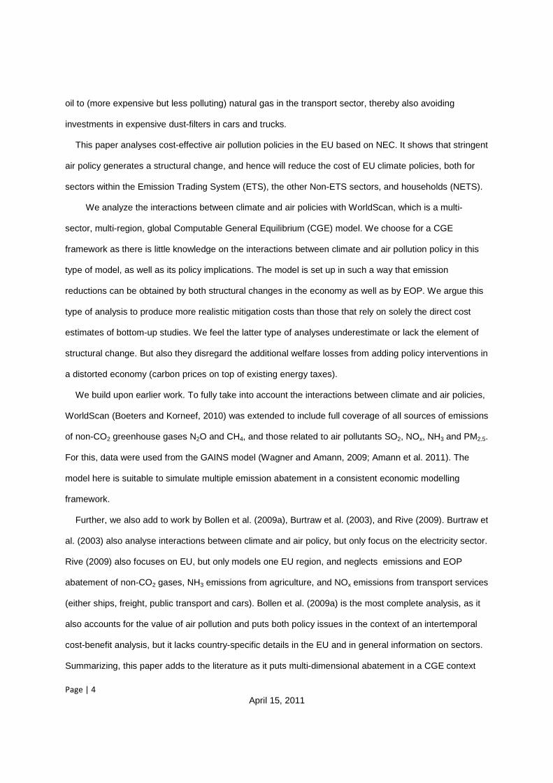
oil to (more expensive but less polluting) natural gas in the transport sector, thereby also avoiding

investments in expensive dust-filters in cars and trucks.

This paper analyses cost-effective air pollution policies in the EU based on NEC. It shows that stringent

air policy generates a structural change, and hence will reduce the cost of EU climate policies, both for

sectors within the Emission Trading System (ETS), the other Non-ETS sectors, and households (NETS).

We analyze the interactions between climate and air policies with WorldScan, which is a multi-

sector, multi-region, global Computable General Equilibrium (CGE) model. We choose for a CGE

framework as there is little knowledge on the interactions between climate and air pollution policy in this

type of model, as well as its policy implications. The model is set up in such a way that emission

reductions can be obtained by both structural changes in the economy as well as by EOP. We argue this

type of analysis to produce more realistic mitigation costs than those that rely on solely the direct cost

estimates of bottom-up studies. We feel the latter type of analyses underestimate or lack the element of

structural change. But also they disregard the additional welfare losses from adding policy interventions in

a distorted economy (carbon prices on top of existing energy taxes).

We build upon earlier work. To fully take into account the interactions between climate and air policies,

WorldScan (Boeters and Korneef, 2010) was extended to include full coverage of all sources of emissions

of non-CO2 greenhouse gases N2O and CH4, and those related to air pollutants SO2, NOx, NH3 and PM2.5.

For this, data were used from the GAINS model (Wagner and Amann, 2009; Amann et al. 2011). The

model here is suitable to simulate multiple emission abatement in a consistent economic modelling

framework.

Further, we also add to work by Bollen et al. (2009a), Burtraw et al. (2003), and Rive (2009). Burtraw et

al. (2003) also analyse interactions between climate and air policy, but only focus on the electricity sector.

Rive (2009) also focuses on EU, but only models one EU region, and neglects emissions and EOP

abatement of non-CO2 gases, NH3 emissions from agriculture, and NOx emissions from transport services

(either ships, freight, public transport and cars). Bollen et al. (2009a) is the most complete analysis, as it

also accounts for the value of air pollution and puts both policy issues in the context of an intertemporal

cost-benefit analysis, but it lacks country-specific details in the EU and in general information on sectors.

Summarizing, this paper adds to the literature as it puts multi-dimensional abatement in a CGE context

Page | 5

April 15, 2011

with sectoral/regional deepening that also allows to analyze actual policy plans in Europe related to both

air pollution and climate change.

Although with the type of model we use we cannot simulate precisely the changes of the productions

processes at the micro-level that could also be relevant for macro-emission abatement. We nevertheless

closely calibrate substance-and-time-specific emission coefficients and Marginal Abatement Cost curves

(MAC’s) of bottom-up studies such as the GAINS model (Amman et al., 2009). Applying these, we can

use our stylized production functions at the sectoral level (including EOP) to simulate the appropriate

price signal for structural changes in economies from combinations of air and climate policies.

Section 2 describes the renewed version WorldScan used for our analyses. This section particularly

focuses on the extensions of the model with respect to emissions of non-CO2 greenhouse gases and air

pollutants. Section 3 presents the policy cases considered. The results of the simulations are presented in

section 4. Finally, in section 5 the main findings are discussed.

2. WorldScan

The macro-economic consequences of specific climate or air policy scenarios are assessed using the

global applied general equilibrium model WorldScan, see Bollen et al. (2004), Lejour et al. (2006), Wobst

et al. (2007); Manders et al. (2008), Hayden et al. (2010), and Bollen et al. (2011). WorldScan data for

the base year 2004 are to a large extent taken from the GTAP-7 database (Badri et al. 2008), which

provides integrated data on bilateral trade flows and input-output accounts for 57 sectors and 113

countries and regions. Here we give only a brief sketch of the aggregation level with respect to regions,

sectors and the main characteristics of the bottom-up representation of the electricity sector. We conclude

with a description of the representation of bottom-up EOP mitigation technologies in the model, which

allows simulating cost-effective reduction of emissions of CO2 from non-energy sources and of CH4, and

N2O from both energy and process-related sources. This extension allows WorldScan to also simulate

what-flexibility with respect to the mitigation of Kyoto-gases. But EOP options are implemented for all air

pollutants, which is relevant for any TSAP.

Page | 6

April 15, 2011

The renewed version of the model enables to simulate the macro-economic impacts of climate and air

policies. In this respect, the main instruments are taxes on pollution and income transfers from acting on

IET, permit trading in ETS and NETS markets, CDM, subsidies to promote renewable energy, and

efficient prices of air pollution.

2.1 Overview

The aggregation of regions and sectors can be flexibly adjusted in WorldScan. We use a version with

23 regions and 18 sectors, listed in Tables 1. Regional disaggregation is relatively fine within Europe, but

coarse outside. The main reason is that the emission ceilings for air pollutants are region/country specific

because of differences in impact of air pollution on human health and ecosystems. Moreover, cost and

potential of control options may differ significantly between regions and/or countries.

Likewise, we focus on a set of sectors accurately representing the heterogeneous characteristics of

activities causing emissions of GHGs and air pollutants, whereas non-polluting sectors are captured in a

more aggregated manner. A distinction is made between sectors taking part in the EU emission trading

system (ETS, consisting of the electricity and the energy intensive sector) and sectors and household

activities which do not participate in the emission trading system (NETS).

Further, we distinguish five agricultural sectors, because of distinct characteristics with respect to

emissions and abatement of air pollutants and of non-CO2 GHGs and also to be able to appropriately

model the production of biofuels (ethanol and bio-diesel). 6,7

Coal , Oil, and Gas are the primary energy sectors.8,9 The Electricity sector is refined with a detailed

electricity technology specification developed by Boeters and Koornneef (2010). Renewable energy is not

6 Rice cultivation, livestock production and fertilizer use are linked the sector Other agricultural activities, which is

hence a major source of emissions of CH4, N2O and NH3.

7 Biodiesel is produced by the sector Vegetable and oils and fats, and ethanol by Sugar beet in Europe and Sugar

cane in Brazil, and Wheat and Corn in the USA.

8 The sector Oil delivers mainly to Petroleum Coal Products, which in turn delivers fuels for one of the two

transport sectors or for consumption of the final good Transport and communication.

Page | 7

April 15, 2011

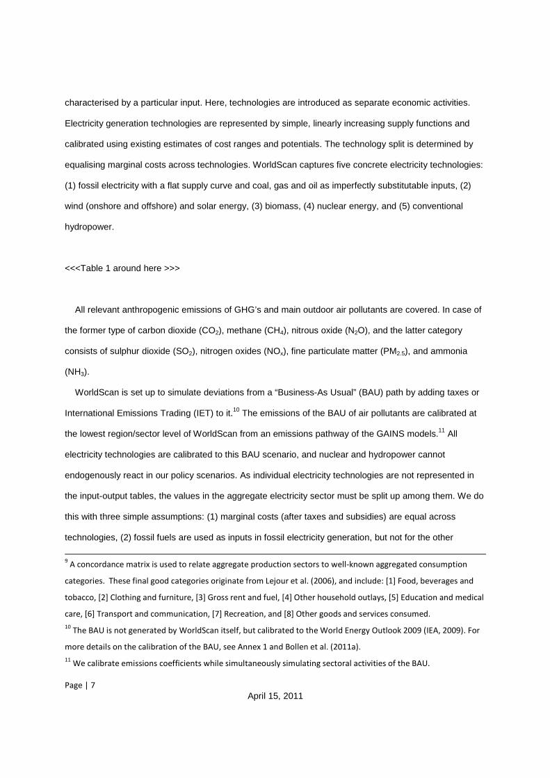
characterised by a particular input. Here, technologies are introduced as separate economic activities.

Electricity generation technologies are represented by simple, linearly increasing supply functions and

calibrated using existing estimates of cost ranges and potentials. The technology split is determined by

equalising marginal costs across technologies. WorldScan captures five concrete electricity technologies:

(1) fossil electricity with a flat supply curve and coal, gas and oil as imperfectly substitutable inputs, (2)

wind (onshore and offshore) and solar energy, (3) biomass, (4) nuclear energy, and (5) conventional

hydropower.

<<<Table 1 around here >>>

All relevant anthropogenic emissions of GHG’s and main outdoor air pollutants are covered. In case of

the former type of carbon dioxide (CO2), methane (CH4), nitrous oxide (N2O), and the latter category

consists of sulphur dioxide (SO2), nitrogen oxides (NOx), fine particulate matter (PM2.5), and ammonia

(NH3).

WorldScan is set up to simulate deviations from a “Business-As Usual” (BAU) path by adding taxes or

International Emissions Trading (IET) to it.10 The emissions of the BAU of air pollutants are calibrated at

the lowest region/sector level of WorldScan from an emissions pathway of the GAINS models.11 All

electricity technologies are calibrated to this BAU scenario, and nuclear and hydropower cannot

endogenously react in our policy scenarios. As individual electricity technologies are not represented in

the input-output tables, the values in the aggregate electricity sector must be split up among them. We do

this with three simple assumptions: (1) marginal costs (after taxes and subsidies) are equal across

technologies, (2) fossil fuels are used as inputs in fossil electricity generation, but not for the other

9 A concordance matrix is used to relate aggregate production sectors to well-known aggregated consumption

categories. These final good categories originate from Lejour et al. (2006), and include: [1] Food, beverages and

tobacco, [2] Clothing and furniture, [3] Gross rent and fuel, [4] Other household outlays, [5] Education and medical

care, [6] Transport and communication, [7] Recreation, and [8] Other goods and services consumed.

10 The BAU is not generated by WorldScan itself, but calibrated to the World Energy Outlook 2009 (IEA, 2009). For

more details on the calibration of the BAU, see Annex 1 and Bollen et al. (2011a).

11 We calibrate emissions coefficients while simultaneously simulating sectoral activities of the BAU.

Page | 8

April 15, 2011

electricity technologies, (3) all other inputs (capital, labour, intermediate goods and services) are used in

proportion to the aggregate shares (as in Boeters and Koornneef, 2010).

2.2 Modelling EOP mitigation technologies

Basic principles of emissions and emission abatement

CO2 emissions can be easily estimated in a CGE model because CO2 is emitted in fixed proportions

with the burning of fossil fuels. This is not true for emissions of other pollutants, e.g. SO2 and NOx. Part of

the emissions of these pollutants are not related to fossil fuel combustion, but caused by, e.g., agriculture

and waste-disposal. A distinction can be made between emissions that are directly related to a specific

input to production (e.g. fossil energy) and those inherent to the production process, independent of the

inputs. These so-called process emissions are related to the output level of a sector.

Generally, emission reductions can be achieved by more efficient use of inputs (e.g. fossil fuels),

substitution across different inputs (e.g. switch from coal to natural gas), investment in emission control

technologies, but also demand reduction and change in the structure of the economy. CGE models have

their strength when it comes to demand shifts and changes in the production structure. For CO2 mitigation

these are most relevant, but for other pollutants EOP is more relevant. The abatement potential and cost

of control options is included in bottom-up engineering models (Markandya, Halsnaes et al., 2001).

Alternative approaches to include emission control in CGE framework

The literature provides a number of approaches for including this kind of emission control in a CGE

model. The general concept is that actors can choose between paying for emissions and investing in

pollution control. Pollution control serves as a substitute to the pollutant emissions, which comes at a

cost. The approaches differ in the way the abatement costs are incorporated in the model. Hyman et al.

(2002) introduce emissions as an input to the production function. The elasticity of substitution between

the emissions and the conventional inputs is estimated to match a marginal abatement cost curve that is

derived from detailed bottom-up studies, e.g. Hyman et al (2002), and Reilly et al. (2002). Gerlagh et al.

(2002) and Dellink et al. (2004) introduce for each pollutant an abatement sector producing mitigation

Page | 9

April 15, 2011

technologies in a region. Emission reductions can be achieved by increasing the input of abatement

goods. The elasticity of substitution is estimated to fit the data on abatement cost of measures as

available from various data sources of technical pollution control measures. Rive (2010) includes

abatement in a CGE model by source-specific technology steps, each step representing groupings of

abatement technologies with similar marginal abatement costs. This offers a flexible treatment that can

incorporate activity- and pollution-specific marginal abatement cost curves of different shapes from

bottom-up studies.

Emissions and emission control in Worldscan

In addition to CO2, we added to WorldScan the major other GHGs (CH4 and N2O). Next, we also added

the most relevant air pollutants SO2, NOx, NH3 and PM2.5 (Amman et al., 2007). For these emissions, not

only fossil fuel combustion is relevant, but also the use of other inputs and the production process in

general. Therefore, we model emissions occurring at different stages of the production process.

Emissions from combustion of energy are calculated as a fixed proportion of the amount of fossil fuel

consumption. Emissions related to the use of chemical fertilizer in agricultural production are similarly

calculated, using the intermediary input from the chemical sector to the agricultural sector as a proxy for

the amount of fertilizer used, illustrated on the nesting of the production function in Figure 2.1. Emissions

that cannot directly be linked to a particular input into the production process are included in the model as

process emissions, i.e. linked to the sectoral output (the top nest of the production function).

<<< Figure 2.1 around here>>>

Reductions in input-related emissions can be achieved by reductions in the use of these inputs, e.g.

through a substitution away from these inputs or by reducing the level of production. Reductions in

process emissions can be achieved by reductions in the level of production. Moreover, as indicated

above, emissions can to a certain extent be reduced by investment in emission control. The possibility to

invest in emission control is introduced in Worldscan by abatement technologies for each type of

Page | 10

April 15, 2011

emissions (input-related and process) in each sector. We omit here indices for region-sector-activity-

substance, and the supply function then reads as:

( )( ) i ii

c a a a pβα γ δ− = ⋅ − − ⋅

∑ (1)

With c(a) the marginal cost of abatement as a function of a, the level of abatement as a percentage of

‘unabated emissions’, i.e. emissions as they would occur without emission control. ā is the maximum level

of abatement, α and β are parameters (both > 0) and γ is a constant that determines the initial level of the

marginal cost c(0). δi are input coefficients and pi prices of the inputs i, indicating the share of the various

inputs required to produce abatement in the cost. The parameters δi are fixed at the shares of the value

inputs of the Capital goods sector. If however, wages rise, then this may also increase the marginal costs

of abatement proportional to the labour share of production of the Capital Goods sector. This functional

form is used because it offers good flexibility to approximate empirical abatement cost curves.12 The total

cost curve is:

( ) ( )11

1 i ii

x x xC a e x p

ββ

α γ δβ

−− − −= ⋅ ⋅ − ⋅ ⋅

− ∑ (2)

with ē the level of emissions as they would occur without emission control. These unabated emissions

are calibrated to a BAU, derived by a bottom-up model (GAINS in this paper), and emission coefficients

are equal to the ratio between emissions of a specific activity and the simulated level of that particular

activity. However, in a policy scenario, we fix the emission coefficient, but not the activity, and therefore

the unabated emissions level ē may change. This feeds into equation 2, and therefore a fixed set of

abatement options may yield different levels of abatement depending whether ē changes compared to the

base year. The commodity and factor input xi in abatement is given by

( )11

1i ii

x x xCx e x

p

ββ

α γ δβ

−− − −∂= = ⋅ ⋅ − ⋅ ⋅ ∂ −

(3)

12

More details on an example of the calibration of MAC’s is given in Annex 2.

Page | 11

April 15, 2011

The optimal abatement level is chosen by equalising the marginal abatement cost and the price of IET

on ETS in case of the climate policy and the uniform air pollution price in case of a country-specific air

pollution target.

The functional form is flexible to approximate a large range of MAC curves. The values of the

parameters ā, α, β, γ and δi are estimated from derived set of MAC curves from GAINS, which is based

on the set of mitigation options of the ranges spanned by Maximum Feasible Target Reductions (MFTR)

in addition to those measures necessary to comply with the Current Legislation in 2020, see Amman et al.

(2010).

Using sector-specific abatement supply allows taking into account differences between sectors in the

possibilities and costs to reduce emissions. This seems to be of particular interest if environmental

policies are differentiating between sectors, such as is the case in the EU where climate policy sets

different targets for sectors within the system of emission trade (ETS) and other sectors. Moreover, as

emission reductions are expressed relative to ‘unabated’ emission levels, changes in emissions that

result from changes in production structure or output levels will proportionally lead to changes in the

abatement potential by emission control options.

Rive (2010) limited EOP abatement to a small number of discrete steps and disregarded sources of

emissions of e.g. the transport sector. By using equation 1 as our format for a MACC, we can deal with

many curves and a wider domain of abatement in sectors and countries without excessive computational

problems. Hence, we are in a better position to put real numbers to the economy-wide allocation of

resources between EOP and structural changes - i.e. to consider air pollution that covers all

anthropogenic emission sources, not just those of some major electric power stations. Nevertheless, we

realize that the equations above are an approximation, but we think we gain in realism of the analysis by

also mimicking the EOP costs of very expensive options (the MFTR potential and a little beyond that

range) and the possible extension (flexibility) and more air pollutants in the analysis (here we also add

non-CO2 gases and NH3).

Page | 12

April 15, 2011

3 Policy cases

Using WorldScan we assess the impacts of several policy variants up to the year 2020, in particular on

emissions and prices of emissions on ETS and NETS markets, on cost-effective air pollutant prices that

meet a pre-specified set of NEC’s, and on competitiveness and welfare. In this paper, welfare is the

Hicksian Equivalent Variation (HEV) to compensate for any losses of utility measured as % of National

Income. Any damage valuation of the environmental state or benefits from improved environmental

quality of policy interventions is not included in this indicator.

<<<Table 2 around here>>>

The air pollution policies are variants of the TSAP, which are presented for EU-27 in Table 2. We

choose three variants of Amman et al. (2007) in increasing order of stringency compared to the BAU:

European Commission (EC), European Parliament (EP), or Cost-Benefit Analysis (CBA).13 They serve to

achieve multiple goals of mitigating mortality from the chronic exposure to particulate matter and ozone,

and the more traditional environmental problems of acidification and eutrophication (see EC, 2011). The

targets are formulated in improvements of the year 2000. The last row of Table 2 refers to an emissions

index of Particulate Matter Surrogate (PMs).14 This indicator reflects the emissions of air pollutants SOx,

NOx, NH3 and PM2.5 relevant for the built-up of outdoor concentration of fine particulate matter. We

choose to present this single indicator, because it summarizes the emissions of air pollution and

determines about 80% of the value estimate of air pollution in Europe, see Holland et al (2007). Although

13

The variants EC, EP, and CBA are taken from Wagner et al. (2010), Amman et al. (2008), and Amman et al. (2005)

respectively. The CBA variant equalizes the difference of direct costs from GAINS and benefits of stringent air

policy at the margin, as reported in Holland et al. (2005). Upon request, we can provide these numbers, but is

beyond the scope of the analysis as presented in this paper.

14 PMS is weighted sum of air pollutants with weights 0.54, 0.88, 2.0, and 0.64 for SOx, NOx, PM2.5, and NH3

respectively. The weights are based on de Leeuw (2000).

Page | 13

April 15, 2011

we only present here the emission targets for EU27, it should be noted that country-and substance-

specific are below this aggregate index (more details in section 4.1).

Mortality from ozone is relevant for air pollution, but is a global externality and hence will be less

affected by EU mitigation plans.15 Table 2 also shows that acidification of ecosystems in Europe will

improve considerably when implementing EC, but be aware that around 55% reduction is already

foreseen in the existing reduction plans (Current Legislation Emissions scenario in Amman et al., 2004).

Other options than mitigation of emissions will be necessary to further lower the acidification in Europe.

Eutrophication is more than acidification driven by the deposition of nitrogen, and as NH3 mitigation is

relatively expensive than SO2 mitigation, the eutrophication improvements (% ecosystem area exceeded)

are lower.

Although we realize that in EU’s Climate and Energy package is already promoted to legislation, we

start with the analytical “clean” option of only air pollution variants based on EU-countries pursuing

multiple national ceilings for air pollutants without having to reduce any GHG’s. We show here the

impacts of the most stringent set of proposed NEC’s, i.e. CBA and the more relaxed variant of EP.

Further, the next three cases introduce the ambitious climate change related pledges made by

countries up to the Copenhagen Climate Change Conference in December 2009, i.e. the third

AMBITIOUS PLEDGES (without air policies) scenario, the fourth AMBITIOUS PLEDGES + CBA variant,

and the fifth policy case relaxes on the ambitions of the air policy: AMBITIOUS PLEDGES + EP.16

15

Although part of the TSAP, we disregard VOC emission reduction plans relevant for ozone formation, because it

hardly affects the analysis. Ozone formation is driven by global changes concentrations of tropospheric CO, from

emissions of CH4, CO2, and then at the regional at the stratosphere affected by emissions of NOx and VOC, see also

Bollen et al. (2009b).

16 Annex I countries ambitiously adopt relatively low caps on GHG-emissions and allow free permit trade amongst

each other. Further, in this scenario China and India impose relative targets for CO2 emission-intensities of 45%

and 25% below 2005 intensities. The EU imposes a 30% GHG emission target, and a 20% share of renewable

energy in final energy use.

Page | 14

April 15, 2011

Next, we analyze the less stringent climate policy of the EU solely implementing its’ Energy and

Climate Package with the renewable target (EU PLEDGE) and without this target (EU GHG).17 These

climate policies are combined with the two earlier air targets, but also extended with EC. Thus, eight

cases are designed: EU PLEDGE + CBA, EU PLEDGE + EP, EU PLEDGE + EC, and EU PLEDGE and

likewise without EU’s renewable target: EU GHG + CBA, EU GHG + EP, and EU GHG + EC, EU GHG.

The AMBITIOUS PLEDGES scenario assumes a completely different institutional setting of climate

policies of the EU PLEDGE, i.e. all Annex 1 countries establish an international IET system leading to a

single uniform carbon price throughout Annex 1. For analytical purposes, we introduce the EU25%

scenario that assumes EU’s GHG reduction to be equal to 25% (instead of 20% of EU PLEDGE).

4 Results

Section 4.1 will analyze marginal costs of abatement of stringent air policies (CBA) for different air

pollutants and welfare impacts for countries. Then, we will relax the stringency of the air targets, and

show how cost-effective structural changes in the economies of the EU-27 induced by air targets reduce

the GHG emissions, and how this compares with Europe’s GHG emission reductions of the EU PLEDGE

and AMBITIOUS PLEDGES. Next, in section 4.2 we will explicitly introduce climate policies, thus enabling

to analyze the interaction between air pollution and climate policies. We will show how prices in ETS and

NETS markets in Europe and welfare are affected through combinations of ambitious and less ambitious

targets for climate policy (30 and 20% targets for GHG and with or without a renewable target for final

energy) and air policy (based on CBA, or proposals by the European Parliament or the European

Commission). Finally, section 4.3 will bring together the results of all policy variants.

17

The EU PLEDGE excludes the use of CDM, but assumes permit trade with one uniform carbon price in ETS and

one in NETS markets in the EU. Again, the EU imposes a targeted 20% share of renewable energy in final energy

use.

Page | 15

April 15, 2011

4.1 Co-benefits of stringent air targets significant

This section presents the impacts in 2020 of imposing national ceilings in different EU countries based

on CBA. We illustrate here the extent to which air policies alone may provoke structural changes in

economies in the EU. We realize that the EU designed its Climate and Energy Package for 2020, but

nevertheless this case serves as a useful guidance for the results of the other cases presented in this

paper. Figure 2 presents the marginal costs of abatement of SO2, NOx, PM2.5, and NH3, and welfare

losses measured as % of national income.

<<<Figure 2 around here>>>

It can be seen that welfare losses will be the largest in the new Member States of the EU (Poland: 3%;

rest of EU-27: 2%). The main reason is that emissions per unit of GDP in these countries will be a factor

of four higher in these countries compared to average of the EU27.18 Hence, the relatively low marginal

costs of abatement (non-zero for al substances) necessary to meet the national ceilings will generate

large distortions in these economies. The next group of countries with more moderate welfare losses are

Italy (1%) and Spain (0.8%). The losses in these countries are mainly driven from the high marginal costs

of abatement compared to the other countries. Germany also has high marginal costs for SO2, but their

welfare losses are less than in Italy and Spain. In Germany the air policy mainly affects the electricity

sector, whereas in Italy and Spain more gasses are taxed and higher costs associated with transport

services. The latter factor will push the welfare losses because of interactions of the air policy with

existing oil taxes in the baseline. For comparison, the numerical importance of this argument is provided

by Klepper and Peterson (2006).

<<<Figure 3 around here>>>

18

For all countries we weight emissions of the different substances according to the Leeuw (2000) to represent

emissions relevant for mortality from the chronic exposure to PM2.5, and divide this aggregate emission index with

the BBP.

Page | 16

April 15, 2011

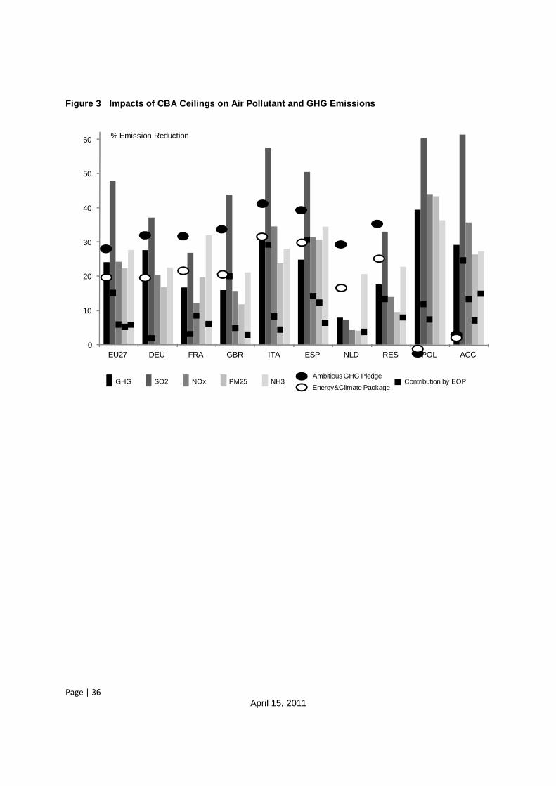
Figure 3 presents for all EU countries in WorldScan the changes in emissions of GHG’s and air

pollutants of the air policy to match the ceilings of the CBA variant. Further there are circles that represent

the emissions reductions implied by the targets of the EU Energy and Climate Package (20%) and

Ambitious Pledges (30%). The results are presented for the same countries as in Figure 2.

It can be seen that stringent air goals have a large indirect impact; it leads to reductions of the GHG

emissions. The air policy targets to reduce 20% of the emissions of NOx, PM2.5, and NH3, and 45% of

SO2, leads to a 25% GHG emission reduction alone! The reason why SO2 emissions reductions are much

larger than for the other substances is that they contribute more significantly to health than the other

substances. The emission reductions for NH3 are significant as well, because ammonia per kg contributes

more significantly to health damages than NOx, and hence EOP options in agriculture are effective as well

(de Leeuw, 2000; Holland et al., 2005). Stringent air policies generate a climate change co-benefit larger

than the climate targets of the Energy and Climate Package can achieve. For each substance it can be

seen that the share contribution of EOP to abatement is limited, keeping in mind that the maximum

feasible reduction is at most a factor of two higher than the simulated outcome. The SO2 emission

reductions are generated by 66% from restructuring of the economy. Rive (2010) comes with a 30-50%

estimate. The reason why we produce more structural changes is that we include more abatement

policies in our BAU, which implies that the low-hanging fruit is excluded in our policy simulations.19 Next

to that, the SO2 emissions reduction effort in this aper is about a factor three higher. Consequently, it may

not be a surprise that there are significant GHG emissions reductions as a co-benefit from these policies.

The co-benefits of efficient stringent air policies come from Germany, Poland and the other accession

countries, because air pollution abatement in these countries is cheaper. Actually, the co-benefit is larger

than the GHG emission reductions pledged by the EU. The other countries can be seen to do less GHG

abatement from their air policies (especially the Netherlands) because of the lack of economies of scale

related to abatement. Despite that EOP to total abatement is large in Eastern European countries, there

19

The SO2 emission level of NEC in Rive (2010) is comparable to the level of our BAU. Hence, the NEC10 calls for an

extra 15% SO2 emission reduction compared to NEC. In this paper, we follow CBA and EP that lead to a 40-50%

emission reduction.

Page | 17

April 15, 2011

seems to be enough inefficiencies in the economy to generate a substantial structural improvement

leading to the simulated co-benefit.

4.2 Also moderate air targets have impacts on climate change policies

The previous section argues that structural changes in the economy will unfold if only air pollution were

to take place (and no climate change policies). In this section we will abandon this assumption, and

analyze the impacts of air targets on climate change policies. Figure 4 presents the changes of emissions

in EU27 related to the GHG’s and air pollutants of various policy scenarios. These scenarios are the air

policies to meet the ceilings of the CBA and EP, and the combinations with climate policy: i.e.

AMBITIOUS PLEDGES with air targets (+EP, +CBA or no air targets). Further, there are circles that

represent the emissions reductions implied by the targets of the AMBITIOUS PLEDGES and EU

PLEDGE.

<<<Figure 4 around here>>>

The AMBITIOUS PLEDGES scenario yields a 15% GHG emission reduction, i.e. half of the necessary

emission reductions will likely be imported from international permit markets against approximately 10

€/tCO2 eq.). Hence, not surprisingly, CBA provokes a larger climate co-benefit (a 22% GHG emission

reduction) than EU’s contribution to the climate in AMBITIOUS PLEDGES scenario (18% GHG emission

reduction). Note also that EP approximates the GHG emission reduction of the AMBITIOUS PLEDGES

case. Adding climate to air policies magnifies GHG emission reductions of the air policy (compare + CBA

with CBA and AMBITIOUS PLEDGES + EP with EP). AMBITIOUS PLEDGES + CBA makes EU

indifferent whether to import or export permits. The internal marginal costs of CO2 abatement goes down

and comes close to the international permit price.

Finally, whereas stringent air targets have climate change co-benefits in the order of the GHG

reductions of the variants of EU PLEDGE and AMBITIOUS PLEDGES, the air quality co-benefits of

Page | 18

April 15, 2011

climate change policies increase only up to 50% of the benefits of the EP variant. In other words, the EU

policy making concentrates with climate change policy, that will only reduce half of the potential number

of premature deaths from air pollution policies of CBA, it is the other policy perspective of air pollution that

will lower the number premature deaths much more effectively, and generates a co-benefit as envisaged

by the climate pledges by the EU.

Next, Figure 5 presents the changes in primary energy use in EU27 from the more relaxed climate

policy resembled by the EU PLEDGE scenario, combined with air ceilings of either the CBA or EP variant.

Primary energy use is split up in oil, gas, coal and all other non-fossil energy carriers (nuclear, wind, sun,

and biomass).

<<<Figure 5 around here>>>

The figure reconfirms the main result of this paper that only achieving air targets without any climate

policy goals will substantially restructure the economy of the EU27. The cost-effective response is to

switch away from fossil fuels and save on energy by 10-15% of total primary energy use (EP and CBA

variant), i.e. fossil energy demand reductions exceed the expansion of the use of non-fossil energy

carriers. The structural changes of the CBA variant can be seen to be larger than those of the EU Pledge.

Also we can see that imposing air targets in line with CBA generates extra reductions in coal (from 5 to

8%) and oil (from 1.5 to 3%), which is driven by the stringency of SO2 target for ETS and NOx and PM2.5

targets for oil in transport sectors. The increase of non-fossil energy demand only applies when the

renewable target is explicitly applied. Otherwise, energy saving seems to be cheaper and dominates the

impacts on energy markets, also reconfirming the results of Boeters et al. (2010). Finally, it can be seen

that gas is affected more than oil in all variants, whereas oil relatively contributes more to pollution

(carbon intensity is approximately 1/3 higher, and for air pollutants this is often much higher). The reason

is that generally the current energy taxes on oil are higher, and hence additional taxation may have a

lower impact on end-user prices, thus lowering also its’ impact on demand.

Page | 19

April 15, 2011

<<<Figure 6 around here>>>

Figure 6 brings together the impacts on welfare and prices on ETS and NETS markets of air policies in

addition to the climate policies (AMBITIOUS PLEDGES and EU PLEDGE with and without renewable

target). The left panel of Figure 6 shows the impacts of air policies on welfare, whereas the right shows

them on the prices in €/ t CO2 eq. The stringency of the air targets are plotted on the x-axis of both

panels; i.e on the left side we start with no air policies (0%), then the EC variant (at around 60% of the

total CBA abatement effort), the EP variant (around 70%), and finally the CBA variant (100%).

We can see that constraining emissions of air pollutants of the EC variant in addition to climate policies

has little impact on welfare and carbon prices (only NETS will go down from 8 to 3 €/ t CO2 eq.). The

welfare losses will be 0.1% point lower without the renewable target. The reason is that this target is

binding, and comes at the expense of an additional subsidy on sustainable energy carriers (solar, wind,

and biomass) amounting up to 20-24% of the user price (either electricity or biofuels).20 The losses of the

AMBITIOUS PLEDGES and EU PLEDGE are approximately the same. On the on hand the carbon price

of the AMBITIOUS PLEDGES is lower than the EU PLEDGE, but on the other hand the terms of trade

gains reduce and the compliance costs (at fixed reductions) will increase as other countries also impose a

climate policy.

Only with more stringent air targets, we can see significant impacts. The welfare losses of the climate

policies (0.4-0.5%) are much increased when imposing an air target (another 0.2% point loss at the most

in the CBA variant). In those scenarios the air targets are binding, and even replace the carbon-induced

distortions. The ETS price will drop from 17 to 11 and 0 €/ t CO2 eq by moving from no air targets to EP

and CBA. ETS as a means of climate policy may become obsolete. This doesn’t mean that innovation in

sustainable energy comes to a halt - as the renewable subsidy will remain at least 20% of the end-user

price, but the distortion becomes different in nature (switching from CO2 to PM2.5 and NOx).21 The NETS

20

Boeters e al. (2010) also estimate the climate costs of the renewable target to be in the range of 0-30% of the

total welfare loss. This paper produces a slightly higher cost estimate than their benchmark case because of lower

shares of renewable energy in the BAU (10 versus 15%).

21 See also a detailed example of coal-fired powerplants in New Member States (excluding Poland) in Annex 1.

Page | 20

April 15, 2011

sectors price response is relatively large to air pollution policies. The main reason is that the transport

sector as part of NETS will be confronted with more binding targets than ETS sectors when also

confronted with air policies.

Summarizing, air targets will lower carbon prices substantially, and especially when air targets are

more binding than EP, then ETS markets may become obsolete. Welfare losses from air policies are

lower than those of climate change policies, especially if they are in addition to climate policies.

4.3 Discussion

Here we bring together the results of the main policy variants. Table 3 presents the impacts of the

various scenarios on welfare, emissions of PMS in the EU (resembling the aggregate representative air

pollutant in this region) and of the global CO2eq, and the ETS permit price.

<<<Table 3 around here >>>

From the climate policy perspective the EU PLEDGE is the benchmark. The next steps for the year

2020 in EU policy could involve extra climate policies or air policies, or a combination of both. In the case

of climate change policies there are two possibilities. Either there will be a 25% cut in GHG emissions in

the same institutional setting as the EU PLEDGE scenario. Or, secondly there will be a 30% cut in GHG

emissions as in the AMBITIOUS PLEDGES scenario. This scenario also assumes the most stringent

targets as pledged by the other Annex 1 countries with full free permit trading amongst these countries. It

can be seen from Table 3 that the impact on global GHG emissions in 2020 in any scenario is limited, and

hence additional climate initiatives does not generate substantial climate change improvements. The co-

benefits are changes in stylized indicator labelled PMS, with extra 2% cut if the EU moves from a 20 to

25% cut in GHG emissions. If however, the EU switches to free permit trading once the carbon coalition

expands, then the trade off occurs with extra global GHG emission reduction of 2.3%, while PMS

emissions increase with 2%point because where-flexibility enables to reduce less on carbon. The

magnitude of the impacts on emissions may be uncertain, but the trade-off is robust if where-flexibility

Page | 21

April 15, 2011

holds. The ETS carbon price drops in the AMBITIOUS PLEDGES scenario to 10 €/ tCO2, while welfare is

unaffected, because lower mitigation costs are offset with lower terms-of-trade gains.

Next, we can see that the EP scenario will reduce the ETS price with 40% and the emissions of PMS

with 10% at lower costs (only 0.05% of NI). Back of the envelope calculus shows that the benefits of

avoided air pollution damages is equal ... % of NI. The EP air pollution policy seems to be superior over

additional climate policies. The EP policy directly aims to bring significant improvements in air quality in

Europe directly affecting people’s health, whereas EU25% is almost as expensive but brings little gains.

This stylized fact also is confirmed by cost-benefit analysis on climate change and air pollution in Bollen

et al. (2009a), and Bollen et al. (2010).

The EU PLEDGE + CBA scenario is a further reduction of PMs emissions and an ambitious step in

environmental policy. At the same time, it can be argued that this step needs to be done as to come in

line with EU’s already 10 years old ambition of a fully clean air for all European citizens. The EU PLEDGE

+ CBA scenario entails a further reduction of the global GHG emissions (0.1% CO2 eq.) with non- binding

GHG targets on ETS markets (more coal reductions) and non-ETS sectors (more oil reductions in

transport) and a binding renewable energy target. Nevertheless, the renewable subsidy reduces with 10%

as more fossil energy reductions enable to reduce also on biomass because the target is formulated as a

20% share and it produces PM emissions. However, the CBA strategy lowers the ETS market price

considerably. Companies under ETS have to comply also with binding targets on SO2, NOx and PM2.5,

and hence new coal fired power stations become too expensive compared to the non-fossil alternatives.

The negotiations within the EU and UN-ECE on air pollution will start this year and finalized by 2014,

and some options for policy can be investigated with the model designed for this paper. With some

modifications the model can also be used to optimally allocate emission ceilings across EU countries that

maximize the health benefits of avoided premature mortality associated with the chronic exposure to

outdoor PM. Although we cannot fully address all the detailed impacts of bottom-models like GAINS, we

nevertheless can shed some light on the structural adjustments in energy markets and the EU-economy

from climate and air policy variants.

Recall from Table 3 that the ceilings based on CBA reduce 53% of number of Years Of Life Lost

(YOLL) in EU27 in the year 2000. The reduction of the number of YOLL in the CBA scenario (compared

Page | 22

April 15, 2011

to the EU PLEDGE scenario) is equal to .. mn YOLL in a period of 10 years. This improvement times the

very conservative estimate median value of YOLL (52000 € per YOLL) is equal 0.?% of NI, which is a

factor x higher than the compliance costs of 0.25% NI. The CBA in addition to the EU PLEDGE pays

back, and further reductions seem feasible. This is also confirmed by Bollen et al. (2009a). Additional

climate policy will be less effective than air policies, because the air pollution improvements are much

smaller almost nothing, and the climate impact (i.e. on global CO2 eq. emissions) is insignificantly

different from the air policy.

In this paper, we focussed on Europe, but employed the WorldScan model, which has global coverage.

The database developed for this paper also calibrates air pollution emission coefficients and EOP

abatement options for China and the US, and can also be used to investigate air pollution policies in a

these regions in a global international trade context. We would expect especially that air pollution policies

in China to impact fossil energy markets and prices, and hence may have an effect on other countries’

economies and environmental policies. This topic will certainly have to be addressed in future research.

Page | 23

April 15, 2011

References

Amann, A. Bertok, I., Cabala, R., Cofala, J., Heyes, C., Gyarfas, F., Klimont, Z., Schöpp, (2004), The

“Current Legislation” and the “Maximum Technically Feasible Reduction” cases for the CAFE baseline

emission projections, version November 10, 2004 (Version 2), CAFE Report Nr. 2, International Institute

for Applied Systems Analysis (IIASA), http://www.iiasa.ac.at/rains/CAFE_files/CAFE-MFR3.pdf.

Amann, A. Bertok, I., Cabala, R., Cofala, J., Heyes, C., Gyarfas, F., Klimont, Z., Schöpp, W., Wagner,

F. (2005), A further emission control scenario for the Clean Air For Europe (CAFE) Programme, version 2

October 2005, CAFE Scenario Analysis Report Nr. 7, International Institute for Applied Systems Analysis

(IIASA), http://www.iiasa.ac.at/rains/CAFE_files/CAFE-D28.pdf.

Amann, M., Bertok, I., Borken-Kleefeld, J., Cofala, J., Heyes, C., Hoeglund Isaksson, L., Klimont,

Z., Purohit, P., Rafaj, P., Schoepp, W., Toth, G., Wagner, F., and Winiwarter W. (2009). Potentials

and Costs for Greenhouse Gas Mitigation in Annex I Countries: Methodology. IIASA Interim Report IR-

09-043 [November 2009].

Amann,M., Bertok, I., Cofala, J., Heyes, C., Klimont, Z., Rafaj, P., Schöpp, W., Wagner, F. (2008),

National Emission Ceilings for 2020 based on the 2008 Climate & Energy Package, NEC Scenario

Analysis Report Nr. 6, IIASA, Vienna, Austria, http://www.iiasa.ac.at/rains/reports/NEC6-final110708.pdf.

Aunan, K., Fang, J., Hu, T., Seip, H., and Vennemo H. (2006), Climate Change and Air Quality—

Measures with Co-Benefits in China, in Environmental Science and Technology,Vol. 40 (16), 2006, pp

4822–4829, DOI: 10.1021/es062994k, Publication Date (Web): August 15, 2006.

Badri, N.G. and T.L. Walmsley (2008), Global trade, assistance, and production: The GTAP 7 data

base, Center for Global Trade Analysis, Purdue University.

Boeters, S., and Kornneef, J. (2010), Supply of renewable energy sources and the cost of EU climate

policy, CPB Discussion Paper 142, CPB Netherlands Bureau for Economic Policy Analysis.

Bollen J., van der Zwaan, B., and Hers, S. (2010), An Integrated Assessment of Climate Change, Air

Pollution, and Energy Security Policy, Energy Policy, Volume 38, Issue 8, Pages 4021-4030.

Bollen, J, van der Zwaan, B, Brink, C, and Eerens, H. (2009a), Local Air Pollution and Global Climate

Change: A Combined Cost-Benefit Analysis, Resource and Energy Economics, Volume 31, Issue 3,

August 2009, Pages 161-181.

Bollen, J., Guay, B., Jamet, S., and Corfee-Morlot, J. (2009b), Co-benefits of Climate Change

Mitigation Policies: Literature Review and New Results, OECD Economics Department Working Paper

No. 693, OECD, Paris.

Page | 24

April 15, 2011

Bollen, J., Koutstaal, P., Veenendaal, P. (2011a), CPB Study on Trade and Climate, April 2011,

European Commission, DG Trade, Brussels, Belgium, forthcoming.

Bollen, J., Brink, C., Koutstaal, P., Veenendaal, P., and Vollebergh, H. (2011b), CPB Policy Brief

05/2011, CPB Netherlands Bureau for Economic Policy Analysis, The Hague, forthcoming.

Bollen, J., M. Mulder and T. Manders, 2004, Four Futures for Energy Markets and Climate Change,

Special Publication 52, CPB Netherlands Bureau for Economic Policy Analysis, The Hague.

Bollen, J.C., 2004, A Trade View on Climate Change Policies, a Multi-Region Multi-Sector Approach”,

PhD thesis, University of Amsterdam, RIVM, Bilthoven.

Burtraw, D., Krupnick, A., Palmer, K., Paul, A., Toman M., and Bloyd, C., 2003, Ancillary Benefits of

Reduced Air Pollution in the US From Moderate Greenhouse Gas Mitigation Policies in the Electricity

Sector, Journal of Environmental Economics and Management 45: 650-673.

CEC (2005). Communication from the Commission to the Council and the European Parliament on a

Thematic Strategy on Air Pollution. SEC(2005) 1132, Commission of the European Communities,

Brussels.

Dellink, Hofkes et al. 2004

Dellink et al. (2004)

EC (2005), Communication from the Commission to the Council and the European Parliament,

Thematic Strategy on air pollution, SEC(2005) 1132 SEC(2005) 1133, COM(2005) 446 final, see also

http://eur-lex.europa.eu/LexUriServ/LexUriServ.do?uri=COM:2005:0446:FIN:EN:PDF.

EC (2011), Commission Staf Working Paper on the implementation of EU Air Quality Policy and

preparing for its comprehensive review, SEC(2011) 342.

EEA (2009), EMEP/EEA air pollutant emission inventory guidebook — 2009, Technical report No

9/2009, 19 Jun 2009, Europe Environment Agency, Copenhagen, Denmark .

Gerlagh et al. (2002)

Hayden, Veenendaal and Zarnić, 2010, Options for International Financing of Climate Change

Mitigation in Developing Countries, Directorate General Economic and Monetary Affairs, ECie.,

http://ec.europa.eu/economy_finance/publications/economic_paper/2010/pdf/ecp406_en.pdf.

Page | 25

April 15, 2011

Holland, M., A. Hunt, F. Hurley, S. Navrud, P. Watkiss, 2004, “Final Methodology Paper (Volume 1) for

the Clean Air for Europe Programme (CAFE)”, European Commission, DG Environment,

AEAT/ED51014/Methodology, Issue 4, Brussels, Belgium.

Holland, M., P. Watkiss, S. Pye, A. Oliveira, and D. Van Regemorter, 2005, “Cost-benefit analysis of

policy option scenarios for the Clean Air for Europe Programme (CAFE)”, European Commission, DG

Environment, AEAT/ED48763001/CBA-CAFE, ABC scenarios, Brussels, Belgium.

Hyman et al. (2002)

IEA (International Energy Agency), 2009, World Energy Outlook 2009, OECD/IEA.

IPCC (2007), Contribution of Working Group I to the Fourth Assessment Report of the

Intergovernmental Panel on Climate Change, 2007, Cambridge University Press, Cambridge, United

Kingdom and New York, NY, USA.

Lejour, A.M., Veenendaal, P., Verweij, G., and van Leeuwen, N., 2006, WorldScan: a Model for

International Economic Policy Analysis, CPB Document 111, The Hague.

Manders T., and Veenendaal, P., 2008, Border tax adjustments and the EU-ETS, A quantitative

assessment, CPB Discussion Paper 171, CPB Netherlands Bureau for Economic Policy Analysis.

Markandya, Halsnaes et al. 2001

OECD, 2009, The Economics of Climate Change Mitigation Policies and Options for Global Action

beyond 2012, Paris.

Reilly et al. 2002).

Rive 2010.

Wagner, F., Amann, M., Bertok, I, Cofala, J., Heyes, C., Klimont, Z., Rafaj,P., and Schöpp, W. (2010),

Baseline Emission Projections and Further Cost-effective Reductions of Air Pollution Impacts in Europe -

A 2010 Perspective, NEC Scenario Analysis Report Nr. 6, IIASA, Vienna, Austria,

http://www.iiasa.ac.at/rains/reports/ NEC7_Interim_report_20100827.pdf.

Wobst, P., N. Anger, P. Veenendaal, V. Alexeeva-Talebi, S. Boeters, N. van Leeuwen, T. Mennel, U.

Oberndorfer and H. Rojas-Romagoza (2007), Competitiveness effects of trading emissions and fostering

technologies to meet the EU Kyoto targets: A quantitative economic assessment, Industrial Policy and

Economic Reforms Papers No.4, DG ENTR.

Page | 26

April 15, 2011

Annex 1: Calibrating WEO 2009 as a Business-As-Usual Scenario

The effects of climate policy depend strongly on the underlying baseline. Our policy scenarios are

based on the baseline of the 2009 World Energy Outlook (WEO, IEA, 2009). With our

baseline we deviate from the WEO-baseline in one respect however. We removed the ETS-caps from the

WEO in order to establish a level playing field for our assessments of the mitigation pledges in an

international context.

The baseline calibration employs trends for population and GDP by region, energy use by region and

energy carrier, and world fossil fuel prices by energy carrier. Population is exogenous, but the other time

series are reproduced by adjusting the model parameters. GDP is targeted by total factor productivity

(differentiated by sector), energy quantities are targeted by energy efficiency, and fuel prices are targeted

by the amount of natural resources available as input to fossil fuel production. In policy variants, total

factor productivity, energy efficiency, and natural sources are fixed exogenously, and GDP, energy use,

and energy prices are endogenous variables.

According to our baseline, global population will continue to expand. Combined with worldwide

economic growth of 2.7% per year global demand for energy will be almost 30% higher in 2020 than in

2004. As described in WEO2009, the effects of the financial and economic crisis are included and have a

large impact on medium term economic growth rates. This expansion predominantly takes place in Non-

Annex I, thus partially reducing the gap in energy consumption per capita with the industrialized countries.

Table 2.1 gives some key overview characteristics of the baseline for the 2004-2020 period. The table

indicates that in the baseline energy- and GHG-intensities are declining worldwide and especially in Non-

Annex I. In principle our baseline follows the fossil fuel price projections of WEO2009 , e.g. the oil price

will reach 100 US$ per barrel in 2020. In Europe, the gas price is expected to lag behind the oil price.

Regional coal prices are expected to remain constant at their 2009 level.

Basically, the main difference between the WEO-baseline and our baseline is increased energy

consumption in the EU (due to the lifting of ETS-caps) and reduced energy consumption elsewhere (due

Page | 27

April 15, 2011

to somewhat higher fossil fuel prices). Table A.1 in the Annex provides the differences in characteristics

of both baselines.

<<Table A.1 around here >>>

PM

1. In Europe no extra renewable energy policies, but already moving 15% by 2020.

2. Air pollution policies in EU, USA, and China

3. We calibrate also the emission-coefficients to derive scenarios for emissions of SO2, NOx, PM2.5, CH4,

N2O, and NH3. Likewise, we also implement cost curves for these pollutants for each sector/region. See

Annex 1 for more details

4. Outside Europe

PM

Page | 28

April 15, 2011

Annex 1: How does EOP work in WorldScan; an example

Environmental policies are implemented in the model by introducing a price on emissions (Lejour et al.,

2006). This emission price makes polluting activities more expensive and will provide an incentive to

reduce these emissions. For emissions directly related to the use of a specific input, such as fossil fuels,

the emission price will in fact cause a rise in the user price of this input. Consequently, this will lead to a

fall in the demand for it and hence a reduction in emissions. For emissions related to sectoral output

levels, the emission price will cause a rise in the output price of the associated product. Consequently,

this will lead to a fall in demand for it and hence in a reduction in emissions. Moreover, if emission control

options are available, these will be implemented up to the level where the marginal cost of emission

control equals the emission price. The emission price can be introduced exogenously, but it is also

possible to set a restriction on emissions in the model. In this case the emission price is endogenously

determined in the model at the level needed to reduce emissions to the predetermined emission target.

For illustrative purposes, we will elaborate the effect of a restriction on emissions of greenhouse gases

and on SO2 emissions for a specific sector, viz. coal-fired power plants in the New Member States

(excluding Poland). Table A.2 presents some relevant results for this sector. In the baseline, 2020

emissions of greenhouse gases are 109 Mton. The EU PLEDGE scenario leads permit trade in ETS

markets leading to a price on GHG emissions of €17/ton CO2-eq, but likewise the renewable target leads

to a renewable price equal to 24% of the user price (not shown in Table A1, but important to keep in

mind) . This emission price is translated into a mark-up on the market price of fossil fuels of 71%, i.e. the

user price of coal for coal-fired power plants in Italy doubles. Also the price of oil and gas rises, so

electricity becomes more expensive and hence the demand for electricity in the New Member States

(excluding Poland) declines by 7%. Because CO2 emissions per energy unit are larger for coal than for oil

and gas, the demand for coal will fall more than proportional: 63% (16 Mtoe). As a result of the decline in

the use of coal, the associated GHG and emissions will decline by 65%. As a co-benefit of climate policy,

SO2 emissions will also be reduced.

Page | 29

April 15, 2011

Reductions in emissions of GHGs from coal-fired power plants in the new Member States (excluding

Poland) can also to some extent be achieved by end-of-pipe abatement. The abatement cost curve in

Figure A.1 shows that at a marginal cost of €31/ton CO2-eq. the N2O emissions from coal-fired power

plants can be reduced by 74%. N2O emissions in the climate policy case amount to 2.4 Mton CO2-eq., so

a reduction of 1.8 Mton can be achieved by implementing end-of-pipe control. So, the overall reduction of

GHG emissions from coal-fired power plants is 75%, which consists of a 74% reduction as a result of

reduced use of coal and an additional 1% reduction as a result of end-of-pipe abatement of SO2

emissions.

<<<Table A1 around here>>>

Policies for air quality improvements are implemented by introducing, in addition to the GHG emission

reduction target, a restriction on emissions of SO2 in the new Member States (excluding Poland). This will

result in an emission price for SO2 of €13/kg SO2. Coal being an important source of SO2 emissions, the

price on SO2 emissions causes the price of coal to increase with 44%. As a result, the demand for coal

will fall by another 11% (74-63%) and consequently also the associated emissions of SO2. As a co-benefit

of this air policy also emissions of GHGs will fall by the same percentage.

The SO2 emission price also induces investment in SO2 emission control. The abatement potential is

limited (about 30% of total SO2 emissions from coal-fired power plants) because to a large extent

emission control already is implemented in the baseline. The abatement cost curve in the right panel of

Figure A.1 indicates that at a marginal cost of €86/kg 19% of the SO2 emissions (i.e. the emissions that

remain after the fall in coal use) can be reduced by emission control.

The fall in GHG emissions makes it much easier to meet the GHG emission reduction target. An

emission price of €11/ton CO2-eq. now is sufficient to meet the ETS reduction target (NB since the ETS

target concerns not only power plants in the new Member States (excluding Poland), but emissions from

all ETS sectors in the EU, this price fall is not uniquely caused by the co-benefit of SO2 reduction in the

coal-fired power plants in the new Member States (excluding Poland); similar co-benefits occur in other

sectors and other countries). Since this price is below the initial marginal cost for end-of-pipe abatement

of N2O (see left panel of Figure 3.1), so no end-of-pipe abatement of GHG emissions will take place. Note

that with climate and air policies together, the coal-fired power plants will contribute more to the total ETS

Page | 30

April 15, 2011

reduction target (i.e. they will have to purchase less emission permits) than in the case with climate policy

only (28 vs. 38 CO2-eq.).

Page | 31

April 15, 2011

Annex 3: Mapping from GAINS to GTAP-VII

<<<here Table A.3>>>

Page | 32

April 15, 2011

a) Non-Annex I regions are denoted in italics b) ETS-sectors and inputs denoted in bold

Table 1 Overview of regions, sectors and technologies and production inputs in WorldScan

Regionsa) Sectorsb) Inputsb) Germany Cereals (Wheat and Cereal Grains NEC) Factors France Oilseeds Low-skilled labour United Kingdom Sugar Crops (Sugar Cane, Sugar Beet) High-skilled labour Italy Other Agriculture Capital Spain Minerals NEC Land Netherlands Oil Natural resources Other EU15 Coal Poland Petroleum Coal Products Primary energy carriers Rest of EU-27 Natural Gas (incl. gas distribution) Coal Norway Electricity Petroleum, coal products

Switzerland Energy Intensive (incl. Chemical Products) Natural gas

Russia Vegetable Oils and Fats Modern biomass Ukraine Consumer Food Products USA Other Consumer Goods Other intermediates

Canada Capital Goods and Durables Cereals (Wheat & Cereal Grains)

Japan Road and Rail Transport Oilseeds

Australia Other Transport (water and air) Sugar Crops (Sugar Cane&Beet)

New Zealand Other Services Other Agriculture Brazil Minerals NEC Middle East and North Africa Electricity Technologies Oil China (incl. Hong Kong)

Conventional fossil (without CCS) Coal

India Fossil with CCS Petroleum Coal Products Rest of the World Nuclear Natural Gas (incl. Distribution) Wind Electricity

Biomass Energy Intensive (incl.

Chemical Products) Substances Hydropower Vegetable Oils and Fats CO2 Consumer Food Products CH4 Conventional biofuel technologies Other Consumer Goods N2O Ethanol Capital Goods and Durables from sugar beet Road and Rail Transport SO2 from sugar cane Other Transport (water and air) NOx from wheat Other Services NH3 from corn Biodiesel PM2.5 Biodiesel Ethanol

Page | 33

April 15, 2011

Figure 1 Production structure with CO2, CH4 and N2O emissions

value-added energy

natural gas (…)CH4

value-added / energy

other inputs

intermediates

land

conventional inputs

output

CH4 N2O

otherintermediates

fertiliseraggregate

N2O fertiliser

(…)

CO2

Page | 34

April 15, 2011

Table 2 Ambition levels for TSAP strategies (% reductions compared to the year 2000)

EC EP CBA Life Years Lost from particulate matter 47 50 53 Acute mortality from ozone 10 16 24 Acidification - ecosystem forest area exceeded 74 79 79 Eutrophication - ecosystem area exceeded 43 46 53 PMS* 55 58 62

Source: Own calculations based on EC (….); PMS is weighted sum of air pollutants with weights equal to 0.54, 0.88, 2.0, and 0.64 for SOx, NOx, PM2.5, and NH3 respectively.

Page | 35

April 15, 2011

Figure 2 Impacts of CBA Ceilings on Emissions price and National Income

Note: SO2 price in / kg SO2

0

10

20

30

40

50

60

70

80

90

100

EU27 DEU FRA GBR ITA ESP NLD RES POL ACC

2000 US$/unit of mass

SO2 NOx PM25 NH3

-3

-2

-1

0

Changes HEV (as% Income)

Page | 36

April 15, 2011

Figure 3 Impacts of CBA Ceilings on Air Pollutant and GHG Emissions

0

10

20

30

40

50

60

EU27 DEU FRA GBR ITA ESP NLD RES POL ACC

% Emission Reduction

GHG SO2 NOx PM25 NH3Ambitious GHG Pledge

Contribution by EOPEnergy&Climate Package

Page | 37

April 15, 2011

Figure 4 Impacts of different Policy Scenarios on Air and GHG Emissions in EU-27

0

10

20

30

40

50

GHG SO2 NOx PM25 NH3 PMs

%

CBA EP Ambitious Pledge + CBA

Ambitious Pledge + EP

Contribution by EOP

Ambitious GHG Pledge

Energy&ClimatePackageAmbitious Pledge

Page | 38

April 15, 2011

Figure 5 Impacts of different Policy Scenarios on Primary Energy Demand in EU-27

- 20

- 15

- 10

- 5

0

5

10

EP CBA EU PLEDGE

CBA

EU PLEDGE EU PLEDGE

- REN CBA

EU PLEDGE

- REN

% of primary energy

coal oil gas other

Page | 39

April 15, 2011

Figure 6 Impacts of Climate & Air Policies on Welfare and Carbon prices in EU-27

Note: 0= no air policies, ≈60%=EC, ≈70% = EP, 100%=CBA

0

10

20

30

40

0 25 50 75 100

€ / t CO2

0

0,2

0,4

0,6

0,8

0 25 50 75 100

%

EU Pledge-REN EU Pledge Ambitious Pledges non-ETS ETS

Losses in Welfare Carbon Prices

Emission Reduction (% of total effort induced by CBA Ceilings)

Page | 40

April 15, 2011

Table 3 Summarizing Climate and Air Policies

PMS (%)

CO2 eq. (%)

Welfare (%)

ETS Price (€ / tCO2 eq.)

Climate Policy

EU Pledge -11 -0,9 -0,5 17

additional changes compared to EU Pledge

+ EU 25% -3 -0,3 -0,08 8

+ Ambitious Pledge 2 -2,3 0,02 -7

+ EC -5 0,0 -0,02 -3

+ EP -10 0,0 -0,05 -6

+ CBA -20 -0,1 -0,27 -17

Air Policy

CBA -29 -0,7 -0,6 -

Page | 41

April 15, 2011

a) Total of coal, refinery products, natural gas, biofuels, commercial biomass and renewable energy

b) GHG-intensity represents the ratio of GHG-emissions and energy consumption

Source: WorldScan

Table A.1 Overview characteristics of the BAU, average annual growth (%), 2004-2020

Population GDP volume

Energy con-sumption a)

GHG emissions

Energy intensity

GHG intensity b)

Annex I 0.3 1.8 0.0 0.1 -1.8 -0.0

EU-27 0.3 1.5 0.6 0.5 -1.0 -0.1

Non-Annex I 1.3 5.4 3.2 3.0 -2.2 -2.9

China (incl. Hong Kong) 0.7 8.2 4.4 3.3 -3.7 -1.1

India 1.3 7.1 4.6 3.2 -2.5 -1.4

World 1.1 2.7 1.6 -1.6 -1.1 -1.7

SO2 NOX PM25 NH3

emissions emissions emissions emissions

Annex I PM

EU-27

Non-Annex I

China (incl. Hong Kong)

India

World

Page | 42

April 15, 2011

Figure A2 Sectoral Contributions to Total Emissions in EU-27

0%

25%

50%

75%

100%GHG SO2 NOx NH3 PM25 PMS

Agriculture Energy Intensive Manufacturing Power

Transport Services Other Consumption

Page | 43

April 15, 2011

Table A.2 Effects of a restriction on emissions of CO2 eq. and SO2 for coal-fired power plants in New Member States (excluding Poland)

BAU EU PLEDGE EU PLEDGE+EP

Coal use (Mtoe) 26 10 (-43%) 7 (-52%) Emission price GHG (€/ton CO2-eq.) 17 11 SO2 (€/kg SO2) 0 13 Mark-up price coal related to price GHG 71% 47% related to price SO2 - 44% Emissions GHG (Mton) 109 38 28 SO2 (kton) 173 63 45 Change emissions GHG -71 (-65%) -82 (-75%) of which - end-of-pipe -2 -1 - structure effects -69 -81 Change emissions SO2 -109 (-63%) -128 (-74%) Of which - end-of-pipe 0 -1 - structure effects -109 -127

Page | 44

April 15, 2011

Figure A.1 Abatement cost curve CO2 and SO2 for coal-fired power plants in Italy

0

10

20

30

40

50

0,0 0,2 0,4 0,6 0,8Emission reduction (%)

Mar

gina

l cos

ts (

€/tC

O2-

eq.)

0

20

40

60

80

100

0,0 0,1 0,2 0,3 0,4Emission reduction (%)

Mar

gina

l cos

t (€/

kg S

O2)

Page | 45

April 15, 2011

Table A.3 Mapping of GAINS sectors to WorldScan sectors

Worldscan sectors GAINS sectors

Cereals, Oilseeds, Sugar crops, Other agriculture Agriculture: Ploughing, tilling, harvesting

Crops left on field

Other transport: agriculture and forestry

Domestic sector - other services, agriculture, forestry, fishing, and non-specified sub-sectors

Cereals Storage and handling: Agricultural products (crops)

Other agriculture Rice cultivation

Agriculture: grassland and soils / organic soils / Livestock / Other

Manure treatment and manure distributed on soils

Forestry

Waste: Agricultural waste burning

Use of mineral N-fertilizer

Minerals NEC Mining: Bauxite, copper, iron ore, zinc ore, manganese ore, other

Storage and handling: Iron ore

Coal, Oil, Natural gas, Petroleum, coal products Fuel combustion in furnaces used in the energy transformation sector

Oil, Natural gas Waste: Flaring in gas and oil industry

Natural gas, Petroleum, coal products Own use of energy sector and losses during production, transmission of final product

Oil Extraction of crude oil

Natural gas (incl. distribution) Extraction, proc. and distribution of gaseous fuels

Transportation of gas

Coal Mining: Brown coal, Hard coal

Storage and handling: Coal

Petroleum, coal products Crude oil & other products - input to Petroleum refineries

Ind. Process: Briquettes production

Conversion: Combustion in boilers

Electricity Power and district heating plants

Industrial power and CHP plants

Energy intensive sectors (incl chemical products), Consumer food product, Other consumer goods, Capital goods and durablesOther Industry

Ind. Process: Carbon black production / Open hearth furnace / Agglomeration plant - pellets / Small industrial and business facilities

Energy intensive sectors (incl chemical products) Iron and Steel IndustryChemical IndustryNon-Ferrous MetalsBuilding Materials IndustryPaper and Pulp IndustryN - fertilizer productionStorage and handling: N,P,K fertilizersWastewater from organic chemical (non-food) manufacturing industryNonenergy use of fuelsStorage and handling: Other industrial products (cement, bauxite, coke)Ind. Process: Production of Cement / Lime / Glass / Bricks / Basic oxygen furnace / Cast iron / Coke oven

Vegetable oils and fats, Consumer food products Food (incl. beverages and tobacco) manufacturing industry

Vegetable oils and fats Fat, edible and non-edible oil extraction

Consumer food products Meat produced

Other consumer goods Textile industryWood and wood products industry

Road and rail transport Road transport - Heavy duty vehicles / Light duty vehicles / Motorcycles / Motorcycles, mopeds and cars with 2-stroke enginesOther transport: rail / offroad / other off-road

Other Transport (water and air) Other transport: domestic air traffic - civil aviation / inland waterways / maritime activities

Other services Domestic sector - commercial and public services

Waste treatment and disposalWaste water treatment (domestic)Municipal solid wasteWaste: Open burning of residential wasteGasoline distributionConstruction activitiesOther transport: mobile sources in construction and industry

Consumption categoriesGross rent and fuel, Other goods and services consumed Domestic sector - residentialTransport and communication Road transport - Light duty vehicles: cars and small buses with 4-stroke engines