machines and máquinas
385
-
Upload
ingmecandres -
Category
Documents
-
view
203 -
download
10
description
the machines and machinery of XXI Century investigation investigación
Transcript of machines and máquinas


MACHINES AND MECHANISMSAPPLIED KINEMATIC ANALYSIS
Fourth Edition
David H. MyszkaUniversity of Dayton
Prentice Hall
Boston Columbus Indianapolis New York San Francisco Upper Saddle RiverAmsterdam Cape Town Dubai London Madrid Milan Munich Paris Montreal Toronto
Delhi Mexico City Sao Paulo Sydney Hong Kong Seoul Singapore Taipei Tokyo

Vice President & Editorial Director:Vernon R. Anthony
Acquisitions Editor: David PloskonkaEditorial Assistant: Nancy KestersonDirector of Marketing: David GesellMarketing Manager: Kara ClarkSenior Marketing Coordinator: Alicia
WozniakMarketing Assistant: Les RobertsSenior Managing Editor: JoEllen GohrAssociate Managing Editor: Alexandrina
Benedicto WolfProduction Editor: Maren L. Miller
Project Manager: Susan HannahsArt Director: Jayne ConteCover Designer: Suzanne Behnke Cover Image: FotoliaFull-Service Project Management:
Hema Latha, Integra Software Services, Pvt Ltd
Composition: Integra Software Services, Pvt Ltd
Text Printer/Bindery: Edwards BrothersCover Printer: Lehigh-Phoenix ColorText Font: 10/12, Minion
Credits and acknowledgments borrowed from other sources and reproduced, withpermission, in this textbook appear on the appropriate page within the text. Unless otherwisestated, all artwork has been provided by the author.
Copyright © 2012, 2005, 2002, 1999 Pearson Education, Inc., publishing as Prentice Hall,One Lake Street, Upper Saddle River, New Jersey, 07458. All rights reserved. Manufacturedin the United States of America. This publication is protected by Copyright, and permissionshould be obtained from the publisher prior to any prohibited reproduction, storage in aretrieval system, or transmission in any form or by any means, electronic, mechanical,photocopying, recording, or likewise. To obtain permission(s) to use material from thiswork, please submit a written request to Pearson Education, Inc., Permissions Department,One Lake Street, Upper Saddle River, New Jersey, 07458.
Many of the designations by manufacturers and seller to distinguish their products areclaimed as trademarks. Where those designations appear in this book, and the publisher wasaware of a trademark claim, the designations have been printed in initial caps or all caps.
Library of Congress Cataloging-in-Publication DataMyszka, David H.
Machines and mechanisms : applied kinematic analysis / David H. Myszka.—4th ed.p. cm.
Includes bibliographical references and index.ISBN-13: 978-0-13-215780-3ISBN-10: 0-13-215780-21. Machinery, Kinematics of. 2. Mechanical movements. I. Title.
TJ175.M97 2012621.8'11—dc22
2010032839
10 9 8 7 6 5 4 3 2 1
ISBN 10: 0-13-215780-2ISBN 13: 978-0-13-215780-3

The objective of this book is to provide the techniquesnecessary to study the motion of machines. A focus is placed onthe application of kinematic theories to real-world machinery.It is intended to bridge the gap between a theoretical study ofkinematics and the application to practical mechanisms.Students completing a course of study using this book shouldbe able to determine the motion characteristics of a machine.The topics presented in this book are critical in machine designprocess as such analyses should be performed on design con-cepts to optimize the motion of a machine arrangement.
This fourth edition incorporates much of the feedbackreceived from instructors and students who used the first threeeditions. Some enhancements include a section introducingspecial-purpose mechanisms; expanding the descriptions ofkinematic properties to more precisely define the property;clearly identifying vector quantities through standard boldfacenotation; including timing charts; presenting analyticalsynthesis methods; clarifying the tables describing cam fol-lower motion; and adding a standard table used for selection ofchain pitch. The end-of-chapter problems have been reviewed.In addition, many new problems have been included.
It is expected that students using this book will have agood background in technical drawing, college algebra, andtrigonometry. Concepts from elementary calculus arementioned, but a background in calculus is not required.Also, knowledge of vectors, mechanics, and computerapplication software, such as spreadsheets, will be useful.However, these concepts are also introduced in the book.
The approach of applying theoretical developments topractical problems is consistent with the philosophy ofengineering technology programs. This book is primarilyoriented toward mechanical- and manufacturing-relatedengineering technology programs. It can be used in eitherassociate or baccalaureate degree programs.
Following are some distinctive features of this book:
1. Pictures and sketches of machinery that containmechanisms are incorporated throughout the text.
2. The focus is on the application of kinematic theories tocommon and practical mechanisms.
3. Both graphical techniques and analytical methods areused in the analysis of mechanisms.
4. An examination copy of Working Model®, a commer-cially available dynamic software package (see Section 2.3on page 32 for ordering information), is extensively usedin this book. Tutorials and problems that utilize thissoftware are integrated into the book.
5. Suggestions for implementing the graphical techniqueson computer-aided design (CAD) systems are includedand illustrated throughout the book.
6. Every chapter concludes with at least one case study.Each case illustrates a mechanism that is used onindustrial equipment and challenges the student todiscuss the rationale behind the design and suggestimprovements.
7. Both static and dynamic mechanism force analysismethods are introduced.
8. Every major concept is followed by an exampleproblem to illustrate the application of the concept.
9. Every Example Problem begins with an introduction of a real machine that relies on the mechanism beinganalyzed.
10. Numerous end-of-chapter problems are consistentwith the application approach of the text. Everyconcept introduced in the chapter has at least oneassociated problem. Most of these problems includethe machine that relies on the mechanism beinganalyzed.
11. Where applicable, end-of-chapter problems areprovided that utilize the analytical methods and arebest suited for programmable devices (calculators,spreadsheets, math software, etc.).
Initially, I developed this textbook after teaching mech-anisms for several semesters and noticing that students didnot always see the practical applications of the material. Tothis end, I have grown quite fond of the case study problemsand begin each class with one. The students refer to this asthe “mechanism of the day.” I find this to be an excellentopportunity to focus attention on operating machinery.Additionally, it promotes dialogue and creates a learningcommunity in the classroom.
Finally, the purpose of any textbook is to guide thestudents through a learning experience in an effectivemanner. I sincerely hope that this book will fulfill this inten-tion. I welcome all suggestions and comments and can bereached at [email protected].
ACKNOWLEDGMENTS
I thank the reviewers of this text for their comments andsuggestions: Dave Brock, Kalamazoo Valley CommunityCollege; Laura Calswell, University of Cincinnati; CharlesDrake, Ferris State University; Lubambala Kabengela,University of North Carolina at Charlotte; Sung Kim,Piedmont Technical College; Michael J. Rider, OhioNorthern University; and Gerald Weisman, University ofVermont.
Dave Myszka
PREFACE
iii
CONTENTS
1 Introduction to Mechanisms andKinematics 1
Objectives 1
1.1 Introduction 1
1.2 Machines and Mechanisms 1
1.3 Kinematics 2
1.4 Mechanism Terminology 2
1.5 Kinematic Diagrams 4
1.6 Kinematic Inversion 8
1.7 Mobility 8
1.7.1 Gruebler’s Equation 8
1.7.2 Actuators and Drivers 12
1.8 Commonly Used Links and Joints 14
1.8.1 Eccentric Crank 14
1.8.2 Pin-in-a-Slot Joint 14
1.8.3 Screw Joint 15
1.9 Special Cases of the Mobility Equation 16
1.9.1 Coincident Joints 16
1.9.2 Exceptions to the Gruebler’sEquation 18
1.9.3 Idle Degrees of Freedom 18
1.10 The Four-Bar Mechanism 19
1.10.1 Grashof ’s Criterion 19
1.10.2 Double Crank 20
1.10.3 Crank-Rocker 20
1.10.4 Double Rocker 20
1.10.5 Change Point Mechanism 20
1.10.6 Triple Rocker 20
1.11 Slider-Crank Mechanism 22
1.12 Special Purpose Mechanisms 22
1.12.1 Straight-Line Mechanisms 22
1.12.2 Parallelogram Mechanisms 22
1.12.3 Quick-Return Mechanisms 23
1.12.4 Scotch Yoke Mechanism 23
1.13 Techniques of Mechanism Analysis 23
1.13.1 Traditional Drafting Techniques 24
1.13.2 CAD Systems 24
1.13.3 Analytical Techniques 24
1.13.4 Computer Methods 24
Problems 25
Case Studies 29
2 Building Computer Models ofMechanisms Using Working Model®
Software 31
Objectives 31
2.1 Introduction 31
2.2 Computer Simulation of Mechanisms 31
2.3 Obtaining Working Model Software 32
2.4 Using Working Model to Model a Four-BarMechanism 32
2.5 Using Working Model to Model a Slider-Crank Mechanism 37
Problems 41
Case Studies 42
3 Vectors 43
Objectives 43
3.1 Introduction 43
3.2 Scalars and Vectors 43
3.3 Graphical Vector Analysis 43
3.4 Drafting Techniques Required in GraphicalVector Analysis 44
3.5 CAD Knowledge Required in Graphical VectorAnalysis 44
3.6 Trigonometry Required in Analytical VectorAnalysis 44
3.6.1 Right Triangle 44
3.6.2 Oblique Triangle 46
3.7 Vector Manipulation 48
3.8 Graphical Vector Addition 48
3.9 Analytical Vector Addition : TriangleMethod 50
3.10 Components of a Vector 52
3.11 Analytical Vector Addition : ComponentMethod 53
3.12 Vector Subtraction 55
3.13 Graphical Vector Subtraction 55
3.14 Analytical Vector Subtraction : TriangleMethod 57
3.15 Analytical Vector Subtraction :Component Method 59
3.16 Vector Equations 60
(- 7)
(- 7)
(- 7)
(- 7)
(+ 7)
(+ 7)
(+ 7)
iv

Contents v
3.17 Application of Vector Equations 62
3.18 Graphical Determination of VectorMagnitudes 63
3.19 Analytical Determination of VectorMagnitudes 66
Problems 67
Case Studies 71
4 Position and DisplacementAnalysis 72
Objectives 72
4.1 Introduction 72
4.2 Position 72
4.2.1 Position of a Point 72
4.2.2 Angular Position of a Link 72
4.2.3 Position of a Mechanism 73
4.3 Displacement 73
4.3.1 Linear Displacement 73
4.3.2 Angular Displacement 73
4.4 Displacement Analysis 74
4.5 Displacement: Graphical Analysis 74
4.5.1 Displacement of a Single DrivingLink 74
4.5.2 Displacement of the Remaining SlaveLinks 75
4.6 Position: Analytical Analysis 79
4.6.1 Closed-Form Position Analysis Equationsfor an In-Line Slider-Crank 81
4.6.2 Closed-Form Position AnalysisEquations for an Offset Slider-Crank 84
4.6.3 Closed-Form Position Equations for aFour-Bar Linkage 87
4.6.4 Circuits of a Four-Bar Linkage 87
4.7 Limiting Positions: Graphical Analysis 87
4.8 Limiting Positions: Analytical Analysis 91
4.9 Transmission Angle 93
4.10 Complete Cycle: Graphical PositionAnalysis 94
4.11 Complete Cycle: Analytical PositionAnalysis 96
4.12 Displacement Diagrams 98
4.13 Coupler Curves 101
Problems 101
Case Studies 108
5 Mechanism Design 109
Objectives 109
5.1 Introduction 109
5.2 Time Ratio 109
5.3 Timing Charts 110
5.4 Design of Slider-Crank Mechanisms 113
5.4.1 In-Line Slider-Crank Mechanism 113
5.4.2 Offset Slider-Crank Mechanism 114
5.5 Design of Crank-Rocker Mechanisms 115
5.6 Design of Crank-Shaper Mechanisms 117
5.7 Mechanism to Move a Link Between TwoPositions 118
5.7.1 Two-Position Synthesis with a PivotingLink 118
5.7.2 Two-Position Synthesis of the Couplerof a Four-Bar Mechanism 118
5.8 Mechanism to Move a Link Between ThreePositions 119
5.9 Circuit and Branch Defects 119
Problems 120
Case Studies 121
6 Velocity Analysis 123
Objectives 123
6.1 Introduction 123
6.2 Linear Velocity 123
6.2.1 Linear Velocity of RectilinearPoints 123
6.2.2 Linear Velocity of a General Point 124
6.2.3 Velocity Profile for Linear Motion 124
6.3 Velocity of a Link 125
6.4 Relationship Between Linear and AngularVelocities 126
6.5 Relative Velocity 128
6.6 Graphical Velocity Analysis: Relative VelocityMethod 130
6.6.1 Points on Links Limited to PureRotation or RectilinearTranslation 130
6.6.2 General Points on a Floating Link 132
6.6.3 Coincident Points on DifferentLinks 135
6.7 Velocity Image 137
6.8 Analytical Velocity Analysis: Relative VelocityMethod 137
6.9 Algebraic Solutions for CommonMechanisms 142
6.9.1 Slider-Crank Mechanism 142
6.9.2 Four-Bar Mechanism 142
6.10 Instantaneous Center of Rotation 142

vi Contents
6.11 Locating Instant Centers 142
6.11.1 Primary Centers 143
6.11.2 Kennedy’s Theorem 144
6.11.3 Instant Center Diagram 144
6.12 Graphical Velocity Analysis: Instant CenterMethod 149
6.13 Analytical Velocity Analysis: Instant CenterMethod 152
6.14 Velocity Curves 155
6.14.1 Graphical Differentiation 157
6.14.2 Numerical Differentiation 159
Problems 161
Case Studies 168
7 Acceleration Analysis 170
Objectives 170
7.1 Introduction 170
7.2 Linear Acceleration 170
7.2.1 Linear Acceleration of RectilinearPoints 170
7.2.2 Constant Rectilinear Acceleration 171
7.2.3 Acceleration and the VelocityProfile 171
7.2.4 Linear Acceleration of a GeneralPoint 173
7.3 Acceleration of a Link 173
7.3.1 Angular Acceleration 173
7.3.2 Constant Angular Acceleration 173
7.4 Normal and Tangential Acceleration 174
7.4.1 Tangential Acceleration 174
7.4.2 Normal Acceleration 175
7.4.3 Total Acceleration 175
7.5 Relative Motion 177
7.5.1 Relative Acceleration 177
7.5.2 Components of RelativeAcceleration 179
7.6 Relative Acceleration Analysis: GraphicalMethod 181
7.7 Relative Acceleration Analysis: AnalyticalMethod 188
7.8 Algebraic Solutions for CommonMechanisms 190
7.8.1 Slider-Crank Mechanism 190
7.8.2 Four-Bar Mechanism 191
7.9 Acceleration of a General Point on a FloatingLink 191
7.10 Acceleration Image 196
7.11 Coriolis Acceleration 197
7.12 Equivalent Linkages 201
7.13 Acceleration Curves 202
7.13.1 Graphical Differentiation 202
7.13.2 Numerical Differentiation 204
Problems 206
Case Studies 213
8 Computer-Aided MechanismAnalysis 215
Objectives 215
8.1 Introduction 215
8.2 Spreadsheets 215
8.3 User-Written Computer Programs 221
8.3.1 Offset Slider-Crank Mechanism 221
8.3.2 Four-Bar Mechanism 221
Problems 222
Case Study 222
9 Cams: Design and KinematicAnalysis 223
Objectives 223
9.1 Introduction 223
9.2 Types of Cams 223
9.3 Types of Followers 224
9.3.1 Follower Motion 224
9.3.2 Follower Position 224
9.3.3 Follower Shape 225
9.4 Prescribed Follower Motion 225
9.5 Follower Motion Schemes 227
9.5.1 Constant Velocity 228
9.5.2 Constant Acceleration 228
9.5.3 Harmonic Motion 228
9.5.4 Cycloidal Motion 230
9.5.5 Combined Motion Schemes 236
9.6 Graphical Disk Cam Profile Design 237
9.6.1 In-Line Knife-Edge Follower 237
9.6.2 In-Line Roller Follower 238
9.6.3 Offset Roller Follower 239
9.6.4 Translating Flat-Faced Follower 240
9.6.5 Pivoted Roller Follower 241
9.7 Pressure Angle 242
9.8 Design Limitations 243
9.9 Analytical Disk Cam Profile Design 243
9.9.1 Knife-Edge Follower 244
9.9.2 In-Line Roller Follower 246
9.9.3 Offset Roller Follower 249
9.9.4 Translating Flat-Faced Follower 249
9.9.5 Pivoted Roller Follower 250

Contents vii
9.10 Cylindrical Cams 251
9.10.1 Graphical Cylindrical Cam ProfileDesign 251
9.10.2 Analytical Cylindrical Cam ProfileDesign 251
9.11 The Geneva Mechanism 252
Problems 254
Case Studies 258
10 Gears: Kinematic Analysis andSelection 260
Objectives 260
10.1 Introduction 260
10.2 Types of Gears 261
10.3 Spur Gear Terminology 262
10.4 Involute Tooth Profiles 264
10.5 Standard Gears 266
10.6 Relationships of Gears in Mesh 268
10.6.1 Center Distance 268
10.6.2 Contact Ratio 269
10.6.3 Interference 270
10.6.4 Undercutting 271
10.6.5 Backlash 272
10.6.6 Operating Pressure Angle 273
10.7 Spur Gear Kinematics 273
10.8 Spur Gear Selection 275
10.8.1 Diametral Pitch 276
10.8.2 Pressure Angle 276
10.8.3 Number of Teeth 276
10.9 Rack and Pinion Kinematics 281
10.10 Helical Gear Kinematics 282
10.11 Bevel Gear Kinematics 285
10.12 Worm Gear Kinematics 286
10.13 Gear Trains 288
10.14 Idler Gears 290
10.15 Planetary Gear Trains 290
10.15.1 Planetary Gear Analysis bySuperposition 291
10.15.2 Planetary Gear Analysis byEquation 293
Problems 295
Case Studies 299
11 Belt and Chain Drives 302
Objectives 302
11.1 Introduction 302
11.2 Belts 302
11.3 Belt Drive Geometry 304
11.4 Belt Drive Kinematics 305
11.5 Chains 308
11.5.1 Types of Chains 308
11.5.2 Chain Pitch 309
11.5.3 Multistrand Chains 309
11.5.4 Sprockets 310
11.6 Chain Drive Geometry 310
11.7 Chain Drive Kinematics 311
Problems 313
Case Studies 315
12 Screw Mechanisms 316
Objectives 316
12.1 Introduction 316
12.2 Thread Features 316
12.3 Thread Forms 316
12.3.1 Unified Threads 317
12.3.2 Metric Threads 317
12.3.3 Square Threads 317
12.3.4 ACME Threads 317
12.4 Ball Screws 317
12.5 Lead 317
12.6 Screw Kinematics 318
12.7 Screw Forces and Torques 322
12.8 Differential Screws 324
12.9 Auger Screws 325
Problems 325
Case Studies 328
13 Static Force Analysis 330
Objectives 330
13.1 Introduction 330
13.2 Forces 330
13.3 Moments and Torques 330
13.4 Laws of Motion 333
13.5 Free-Body Diagrams 333
13.5.1 Drawing a Free-Body Diagram 333
13.5.2 Characterizing Contact Forces 333
13.6 Static Equilibrium 335
13.7 Analysis of a Two-Force Member 335
13.8 Sliding Friction Force 341
Problems 343
Case Study 345
14 Dynamic Force Analysis 346
Objectives 346
14.1 Introduction 346

viii Contents
14.2 Mass and Weight 346
14.3 Center of Gravity 347
14.4 Mass Moment of Inertia 348
14.4.1 Mass Moment of Inertia of BasicShapes 348
14.4.2 Radius of Gyration 350
14.4.3 Parallel Axis Theorem 350
14.4.4 Composite Bodies 351
14.4.5 Mass Moment of Inertia—Experimental Determination 352
14.5 Inertial Force 352
14.6 Inertial Torque 357
Problems 363
Case Study 366
Answers to Selected Even-Numbered Problems 367
References 370
Index 371

of different drivers. This information sets guidelines for therequired movement of the wipers. Fundamental decisionsmust be made on whether a tandem or opposed wipe pat-tern better fits the vehicle. Other decisions include theamount of driver- and passenger-side wipe angles and thelocation of pivots. Figure 1.1 illustrates a design concept,incorporating an opposed wiper movement pattern.
Once the desired movement has been established, anassembly of components must be configured to move thewipers along that pattern. Subsequent tasks include analyz-ing other motion issues such as timing of the wipers andwhipping tendencies. For this wiper system, like mostmachines, understanding and analyzing the motion is neces-sary for proper operation. These types of movement andmotion analyses are the focus of this textbook.
Another major task in designing machinery is deter-mining the effect of the forces acting in the machine. Theseforces dictate the type of power source that is required tooperate the machine. The forces also dictate the requiredstrength of the components. For instance, the wiper systemmust withstand the friction created when the windshield iscoated with sap after the car has been parked under a tree.This type of force analysis is a major topic in the latterportion of this text.
1.2 MACHINES AND MECHANISMS
Machines are devices used to alter, transmit, and direct forcesto accomplish a specific objective. A chain saw is a familiarmachine that directs forces to the chain with the objective ofcutting wood. A mechanism is the mechanical portion of a
O B J E C T I V E S
Upon completion of this chapter, the student will be able to:
1. Explain the need for kinematic analysis ofmechanisms.
2. Define the basic components that comprise amechanism.
3. Draw a kinematic diagram from a view of a complexmachine.
4. Compute the number of degrees of freedom of amechanism.
5. Identify a four-bar mechanism and classify it accordingto its possible motion.
6. Identify a slider-crank mechanism.
C H A P T E R
O N E
INTRODUCTION TO MECHANISMS AND KINEMATICS
1.1 INTRODUCTION
Imagine being on a design and development team. The teamis responsible for the design of an automotive windshieldwiper system. The proposed vehicle is a sports model withan aerodynamic look and a sloped windshield. Of course, thepurpose of this wiper system is to clean water and debrisfrom the windshield, giving clear vision to the driver.Typically, this is accomplished by sweeping a pair of wipersacross the glass.
One of the first design tasks is determining appropriatemovements of the wipers. The movements must be suffi-cient to ensure that critical portions of the windshield arecleared. Exhaustive statistical studies reveal the view ranges
FIGURE 1.1 Proposed windshield wiper movements.
1
machine that has the function of transferring motion andforces from a power source to an output. It is the heart of amachine. For the chain saw, the mechanism takes power froma small engine and delivers it to the cutting edge of the chain.
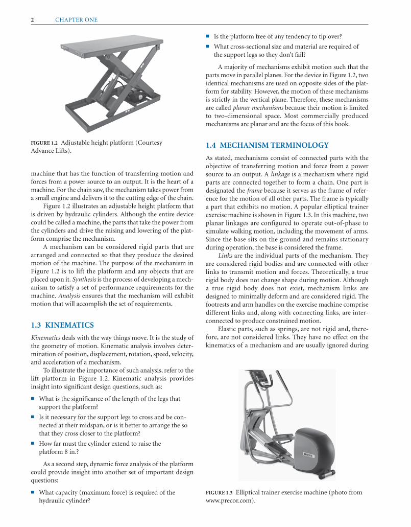
Figure 1.2 illustrates an adjustable height platform thatis driven by hydraulic cylinders. Although the entire devicecould be called a machine, the parts that take the power fromthe cylinders and drive the raising and lowering of the plat-form comprise the mechanism.
A mechanism can be considered rigid parts that arearranged and connected so that they produce the desiredmotion of the machine. The purpose of the mechanism inFigure 1.2 is to lift the platform and any objects that areplaced upon it. Synthesis is the process of developing a mech-anism to satisfy a set of performance requirements for themachine. Analysis ensures that the mechanism will exhibitmotion that will accomplish the set of requirements.
1.3 KINEMATICS
Kinematics deals with the way things move. It is the study ofthe geometry of motion. Kinematic analysis involves deter-mination of position, displacement, rotation, speed, velocity,and acceleration of a mechanism.
To illustrate the importance of such analysis, refer to thelift platform in Figure 1.2. Kinematic analysis providesinsight into significant design questions, such as:
� What is the significance of the length of the legs thatsupport the platform?
� Is it necessary for the support legs to cross and be con-nected at their midspan, or is it better to arrange the sothat they cross closer to the platform?
� How far must the cylinder extend to raise the platform 8 in.?
As a second step, dynamic force analysis of the platformcould provide insight into another set of important designquestions:
� What capacity (maximum force) is required of thehydraulic cylinder?
2 CHAPTER ONE
� Is the platform free of any tendency to tip over?
� What cross-sectional size and material are required ofthe support legs so they don’t fail?
A majority of mechanisms exhibit motion such that theparts move in parallel planes. For the device in Figure 1.2, twoidentical mechanisms are used on opposite sides of the plat-form for stability. However, the motion of these mechanismsis strictly in the vertical plane. Therefore, these mechanismsare called planar mechanisms because their motion is limitedto two-dimensional space. Most commercially producedmechanisms are planar and are the focus of this book.
1.4 MECHANISM TERMINOLOGY
As stated, mechanisms consist of connected parts with theobjective of transferring motion and force from a powersource to an output. A linkage is a mechanism where rigidparts are connected together to form a chain. One part isdesignated the frame because it serves as the frame of refer-ence for the motion of all other parts. The frame is typicallya part that exhibits no motion. A popular elliptical trainerexercise machine is shown in Figure 1.3. In this machine, twoplanar linkages are configured to operate out-of-phase tosimulate walking motion, including the movement of arms.Since the base sits on the ground and remains stationaryduring operation, the base is considered the frame.
Links are the individual parts of the mechanism. Theyare considered rigid bodies and are connected with otherlinks to transmit motion and forces. Theoretically, a truerigid body does not change shape during motion. Althougha true rigid body does not exist, mechanism links aredesigned to minimally deform and are considered rigid. Thefootrests and arm handles on the exercise machine comprisedifferent links and, along with connecting links, are inter-connected to produce constrained motion.
Elastic parts, such as springs, are not rigid and, there-fore, are not considered links. They have no effect on thekinematics of a mechanism and are usually ignored during
FIGURE 1.2 Adjustable height platform (Courtesy Advance Lifts).
FIGURE 1.3 Elliptical trainer exercise machine (photo fromwww.precor.com).

Introduction to Mechanisms and Kinematics 3
Link 1
Link 2
(a) Cam joint (b) Gear joint
Link 2
Link 1
(a) Pin (b) Sliding
Link 1Link 2
FIGURE 1.4 Primary joints: (a) Pin and (b) Sliding.
FIGURE 1.5 Higher-order joints: (a) Cam joint and (b) Gear joint.
kinematic analysis. They do supply forces and must beincluded during the dynamic force portion of analysis.
A joint is a movable connection between links and allowsrelative motion between the links. The two primary joints, alsocalled full joints, are the revolute and sliding joints. Therevolute joint is also called a pin or hinge joint. It allows purerotation between the two links that it connects. The slidingjoint is also called a piston or prismatic joint. It allows linearsliding between the links that it connects. Figure 1.4 illustratesthese two primary joints.
A cam joint is shown in Figure 1.5a. It allows for bothrotation and sliding between the two links that it connects.Because of the complex motion permitted, the cam connec-tion is called a higher-order joint, also called half joint. A gearconnection also allows rotation and sliding between twogears as their teeth mesh. This arrangement is shown inFigure 1.5b. The gear connection is also a higher-order joint.
A simple link is a rigid body that contains only twojoints, which connect it to other links. Figure 1.6a illustratesa simple link. A crank is a simple link that is able to complete
(a) Simple link (b) Complex link
FIGURE 1.6 Links: (a) Simple link and (b) Complex link.

4 CHAPTER ONE
FIGURE 1.7 Articulated robot (Courtesy of Motoman Inc.).
FIGURE 1.8 Two-armed synchro loader (Courtesy PickOmatic Systems,Ferguson Machine Co.).
a full rotation about a fixed center. A rocker is a simple linkthat oscillates through an angle, reversing its direction at cer-tain intervals.
A complex link is a rigid body that contains more thantwo joints. Figure 1.6b illustrates a complex link. A rockerarm is a complex link, containing three joints, that is pivotednear its center. A bellcrank is similar to a rocker arm, but isbent in the center. The complex link shown in Figure 1.6b isa bellcrank.
A point of interest is a point on a link where the motionis of special interest. The end of the windshield wiper, previ-ously discussed, would be considered a point of interest.Once kinematic analysis is performed, the displacement,velocity, and accelerations of that point are determined.
The last general component of a mechanism is theactuator. An actuator is the component that drives themechanism. Common actuators include motors (electricand hydraulic), engines, cylinders (hydraulic and pneu-matic), ball-screw motors, and solenoids. Manually oper-ated machines utilize human motion, such as turning acrank, as the actuator. Actuators will be discussed further inSection 1.7.
Linkages can be either open or closed chains. Each link ina closed-loop kinematic chain is connected to two or moreother links. The lift in Figure 1.2 and the elliptical trainer ofFigure 1.3 are closed-loop chains. An open-loop chain willhave at least one link that is connected to only one otherlink. Common open-loop linkages are robotic arms asshown in Figure 1.7 and other “reaching” machines such asbackhoes and cranes.
1.5 KINEMATIC DIAGRAMS
In analyzing the motion of a machine, it is often difficult tovisualize the movement of the components in a full assemblydrawing. Figure 1.8 shows a machine that is used to handle
parts on an assembly line. A motor produces rotational power,which drives a mechanism that moves the arms back and forthin a synchronous fashion. As can be seen in Figure 1.8, a picto-rial of the entire machine becomes complex, and it is difficultto focus on the motion of the mechanism under consideration.
(This item omitted from WebBook edition)

Introduction to Mechanisms and Kinematics 5
TABLE 1.1 Symbols Used in Kinematic Diagrams
Component Typical Form Kinematic Representation
Simple Link
Simple Link(with pointof interest)
Complex Link
Pin Joint
It is easier to represent the parts in skeleton form so thatonly the dimensions that influence the motion of themechanism are shown. These “stripped-down” sketches ofmechanisms are often referred to as kinematic diagrams. Thepurpose of these diagrams is similar to electrical circuitschematic or piping diagrams in that they represent vari-ables that affect the primary function of the mechanism.
Table 1.1 shows typical conventions used in creating kine-matic diagrams.
A kinematic diagram should be drawn to a scale pro-portional to the actual mechanism. For convenient refer-ence, the links are numbered, starting with the frame aslink number 1. To avoid confusion, the joints should belettered.
(continued)

FIGURE 1.9 Shear press for Example Problem 1.1.
6 CHAPTER ONE
EXAMPLE PROBLEM 1.1
Figure 1.9 shows a shear that is used to cut and trim electronic circuit board laminates. Draw a kinematic
diagram.
TABLE 1.1 (Continued)
Component Typical Form Kinematic Representation
Slider Joint
Cam Joint
Gear Joint
SOLUTION: 1. Identify the Frame
The first step in constructing a kinematic diagram is to decide the part that will be designated as the frame.
The motion of all other links will be determined relative to the frame. In some cases, its selection is obvious as
the frame is firmly attached to the ground.
In this problem, the large base that is bolted to the table is designated as the frame. The motion of all other
links is determined relative to the base. The base is numbered as link 1.
Link 1
Link 2

FIGURE 1.11 Vise grips for Example Problem 1.2.
FIGURE 1.10 Kinematic diagram for Example Problem 1.1.
Introduction to Mechanisms and Kinematics 7
A
B
C
D
X
43
1
2
2. Identify All Other Links
Careful observation reveals three other moving parts:
Link 2: Handle
Link 3: Cutting blade
Link 4: Bar that connects the cutter with the handle
3. Identify the Joints
Pin joints are used to connect link 1 to 2, link 2 to 3, and link 3 to 4. These joints are lettered A through C. In
addition, the cutter slides up and down, along the base. This sliding joint connects link 4 to 1, and is lettered D.
4. Identify Any Points of Interest
Finally, the motion of the end of the handle is desired. This is designated as point of interest X.
5. Draw the Kinematic Diagram
The kinematic diagram is given in Figure 1.10.
EXAMPLE PROBLEM 1.2
Figure 1.11 shows a pair of vise grips. Draw a kinematic diagram.
SOLUTION: 1. Identify the Frame
The first step is to decide the part that will be designated as the frame. In this problem, no parts are attached to
the ground. Therefore, the selection of the frame is rather arbitrary.
The top handle is designated as the frame. The motion of all other links is determined relative to the top
handle. The top handle is numbered as link 1.
2. Identify All Other Links
Careful observation reveals three other moving parts:
Link 2: Bottom handle
Link 3: Bottom jaw
Link 4: Bar that connects the top and bottom handle
3. Identify the Joints
Four pin joints are used to connect these different links (link 1 to 2, 2 to 3, 3 to 4, and 4 to 1). These joints are
lettered A through D.
4. Identify Any Points of Interest
The motion of the end of the bottom jaw is desired. This is designated as point of interest X. Finally, the motion
of the end of the lower handle is also desired. This is designated as point of interest Y.

8 CHAPTER ONE
(a) Single degree-of-freedom (M = 1) (b) Locked mechanism (M = 0) (c) Multi-degree-of-freedom (M = 2)
FIGURE 1.13 Mechanisms and structures with varying mobility.
5. Draw the Kinematic Diagram
The kinematic diagram is given in Figure 1.12.
1.6 KINEMATIC INVERSION
Absolute motion is measured with respect to a stationaryframe. Relative motion is measured for one point or linkwith respect to another link. As seen in the previous exam-ples, the first step in drawing a kinematic diagram isselecting a member to serve as the frame. In some cases,the selection of a frame is arbitrary, as in the vise gripsfrom Example Problem 1.2. As different links are chosen asa frame, the relative motion of the links is not altered, butthe absolute motion can be drastically different. Formachines without a stationary link, relative motion isoften the desired result of kinematic analysis.
In Example Problem 1.2, an important result of kine-matic analysis is the distance that the handle must be movedin order to open the jaw. This is a question of relative posi-tion of the links: the handle and jaw. Because the relativemotion of the links does not change with the selection of aframe, the choice of a frame link is often not important.Utilizing alternate links to serve as the fixed link is termedkinematic inversion.
1.7 MOBILITY
An important property in mechanism analysis is the number ofdegrees of freedom of the linkage. The degree of freedom is thenumber of independent inputs required to precisely positionall links of the mechanism with respect to the ground. It canalso be defined as the number of actuators needed to operatethe mechanism. A mechanism actuator could be manuallymoving one link to another position, connecting a motor to theshaft of one link, or pushing a piston of a hydraulic cylinder.
The number of degrees of freedom of a mechanism isalso called the mobility, and it is given the symbol . WhenM
the configuration of a mechanism is completely defined bypositioning one link, that system has one degree of freedom.Most commercially produced mechanisms have one degreeof freedom. In constrast, robotic arms can have three, ormore, degrees of freedom.
1.7.1 Gruebler’s Equation
Degrees of freedom for planar linkages joined with commonjoints can be calculated through Gruebler’s equation:
where:
jh total number of higher-order joints (cam or gear joints)
As mentioned, most linkages used in machines have onedegree of freedom. A single degree-of-freedom linkage isshown in Figure 1.13a.
Linkages with zero, or negative, degrees of freedom aretermed locked mechanisms. These mechanisms are unableto move and form a structure. A truss is a structure com-posed of simple links and connected with pin joints andzero degrees of freedom. A locked mechanism is shown inFigure 1.13b.
Linkages with multiple degrees of freedom need morethan one driver to precisely operate them. Commonmulti-degree-of-freedom mechanisms are open-loopkinematic chains used for reaching and positioning, suchas robotic arms and backhoes. In general, multi-degree-of-freedom linkages offer greater ability to precisely positiona link. A multi-degree-of-freedom mechanism is shown inFigure 1.13c.
=
jp = total number of primary joints (pins or sliding joints)
n = total number of links in the mechanism
M = degrees of freedom = 3(n - 1) - 2jp - jh
FIGURE 1.12 Kinematic diagram for Example Problem 1.2.
2
41
AD
Y
C B
X3

Introduction to Mechanisms and Kinematics 9
FIGURE 1.14 Toggle clamp for Example Problem 1.3.
EXAMPLE PROBLEM 1.3
Figure 1.14 shows a toggle clamp. Draw a kinematic diagram, using the clamping jaw and the handle as points of
interest. Also compute the degrees of freedom for the clamp.
SOLUTION: 1. Identify the Frame
The component that is bolted to the table is designated as the frame. The motion of all other links is determined
relative to this frame. The frame is numbered as link 1.
2. Identify All Other Links
Careful observation reveals three other moving parts:
Link 2: Handle
Link 3: Arm that serves as the clamping jaw
Link 4: Bar that connects the clamping arm and handle
3. Identify the Joints
Four pin joints are used to connect these different links (link 1 to 2, 2 to 3, 3 to 4, and 4 to 1). These joints are
lettered A through D.
4. Identify Any Points of Interest
The motion of the clamping jaw is desired. This is designated as point of interest X. Finally, the motion of the
end of the handle is also desired. This is designated as point of interest Y.
5. Draw the Kinematic Diagram
The kinematic diagram is detailed in Figure 1.15.
1
4
3
X
A
BC
D
Y
2
FIGURE 1.15 Kinematic diagram for Example Problem 1.3.
6. Calculate Mobility
Having four links and four pin joints,
n = 4, jp = 4 pins, jh = 0

10 CHAPTER ONE
1
2
4
3C
A
B D
X
FIGURE 1.17 Kinematic diagram for Example Problem 1.4.
FIGURE 1.16 Can crusher for Example Problem 1.4.
and
With one degree of freedom, the clamp mechanism is constrained. Moving only one link, the handle, precisely
positions all other links in the clamp.
M = 3(n - 1) - 2jp - j h = 3(4 - 1) - 2(4) - 0 = 1
EXAMPLE PROBLEM 1.4
Figure 1.16 shows a beverage can crusher used to reduce the size of cans for easier storage prior to recycling. Draw a
kinematic diagram, using the end of the handle as a point of interest. Also compute the degrees of freedom for
the device.
SOLUTION: 1. Identify the Frame
The back portion of the device serves as a base and can be attached to a wall. This component is designated
as the frame. The motion of all other links is determined relative to this frame. The frame is numbered as
link 1.
2. Identify All Other Links
Careful observation shows a planar mechanism with three other moving parts:
Link 2: Handle
Link 3: Block that serves as the crushing surface
Link 4: Bar that connects the crushing block and handle
3. Identify the Joints
Three pin joints are used to connect these different parts. One pin connects the handle to the base. This joint is
labeled as A. A second pin is used to connect link 4 to the handle. This joint is labeled B. The third pin connects
the crushing block and link 4. This joint is labeled C.
The crushing block slides vertically during operation; therefore, a sliding joint connects the crushing block
to the base. This joint is labeled D.
4. Identify Any Points of Interest
The motion of the handle end is desired. This is designated as point of interest X.
5. Draw the Kinematic Diagram
The kinematic diagram is given in Figure 1.17.

Introduction to Mechanisms and Kinematics 11
FIGURE 1.18 Shear press for Example Problem 1.5.
6. Calculate Mobility
It was determined that there are four links in this mechanism. There are also three pin joints and one slider joint.
Therefore,
and
With one degree of freedom, the can crusher mechanism is constrained. Moving only one link, the handle, precisely
positions all other links and crushes a beverage can placed under the crushing block.
M = 3(n - 1) - 2jp - j h = 3(4 - 1) - 2(4) - 0 = 1
n = 4, jp = (3 pins + 1 slider) = 4, jh = 0
EXAMPLE PROBLEM 1.5
Figure 1.18 shows another device that can be used to shear material. Draw a kinematic diagram, using the
end of the handle and the cutting edge as points of interest. Also, compute the degrees of freedom for the
shear press.
SOLUTION: 1. Identify the Frame
The base is bolted to a working surface and can be designated as the frame. The motion of all other links is de-
termined relative to this frame. The frame is numbered as link 1.
2. Identify All Other Links
Careful observation reveals two other moving parts:
Link 2: Gear/handle
Link 3: Cutting lever
3. Identify the Joints
Two pin joints are used to connect these different parts. One pin connects the cutting lever to the frame.
This joint is labeled as A. A second pin is used to connect the gear/handle to the cutting lever. This joint is
labeled B.
The gear/handle is also connected to the frame with a gear joint. This higher-order joint is
labeled C.
4. Identify Any Points of Interest
The motion of the handle end is desired and is designated as point of interest X. The motion of the cutting surface is
also desired and is designated as point of interest Y.
5. Draw the Kinematic Diagram
The kinematic diagram is given in Figure 1.19.

12 CHAPTER ONE
2
1
YA
CB
X
3
FIGURE 1.19 Kinematic diagram for Example Problem 1.5.
6. Calculate Mobility
To calculate the mobility, it was determined that there are three links in this mechanism. There are also two pin
joints and one gear joint. Therefore,
and
With one degree of freedom, the shear press mechanism is constrained. Moving only one link, the handle,
precisely positions all other links and brings the cutting edge onto the work piece.
M = 3(n - 1) - 2jp - jh = 3(3 - 1) - 2(2) - 1 = 1
n = 3 jp = (2 pins) = 2 jh = (1 gear connection) = 1
1.7.2 Actuators and Drivers
In order to operate a mechanism, an actuator, or driverdevice, is required to provide the input motion and energy.To precisely operate a mechanism, one driver is required foreach degree of freedom exhibited. Many different actuatorsare used in industrial and commercial machines and mecha-nisms. Some of the more common ones are given below:
Electric motors (AC) provide the least expensive wayto generate continuous rotary motion. However,they are limited to a few standard speeds that are afunction of the electric line frequency. In NorthAmerica the line frequency is 60 Hz, which corre-sponds to achievable speeds of 3600, 1800, 900, 720,and 600 rpm. Single-phase motors are used in resi-dential applications and are available from 1/50 to2 hp. Three-phase motors are more efficient, butmostly limited to industrial applications becausethey require three-phase power service. They areavailable from 1/4 to 500 hp.
Electric motors (DC) also produce continuous rotarymotion. The speed and direction of the motion canbe readily altered, but they require power from a gen-erator or a battery. DC motors can achieve extremelyhigh speeds––up to 30,000 rpm. These motors aremost often used in vehicles, cordless devices, or inapplications where multiple speeds and directionalcontrol are required, such as a sewing machine.
Engines also generate continuous rotary motion. Thespeed of an engine can be throttled within a rangeof approximately 1000 to 8000 rpm. They are apopular and highly portable driver for high-powerapplications. Because they rely on the combustionof fuel, engines are used to drive machines thatoperate outdoors.
Servomotors are motors that are coupled with a con-troller to produce a programmed motion or hold afixed position. The controller requires sensors on thelink being moved to provide feedback information onits position, velocity, and acceleration. These motorshave lower power capacity than nonservomotors andare significantly more expensive, but they can be usedfor machines demanding precisely guided motion,such as robots.
Air or hydraulic motors also produce continuousrotary motion and are similar to electric motors, buthave more limited applications. This is due to theneed for compressed air or a hydraulic source. Thesedrive devices are mostly used within machines, suchas construction equipment and aircraft, where high-pressure hydraulic fluid is available.
Hydraulic or pneumatic cylinders are common com-ponents used to drive a mechanism with a limitedlinear stroke. Figure 1.20a illustrates a hydrauliccylinder. Figure 1.20b shows the common kinematicrepresentation for the cylinder unit.
Introduction to Mechanisms and Kinematics 13
Pin jointLink A(cylinder)
Pin joint
Slidingjoint
Link B(piston/rod)
Cylinder
(a) (b)
RodPiston
FIGURE 1.21 Outrigger for Example Problem 1.6.
FIGURE 1.20 Hydraulic cylinder.
The cylinder unit contains a rod and piston assemblythat slides relative to a cylinder. For kinematic pur-poses, these are two links (piston/rod and cylinder),connected with a sliding joint. In addition, thecylinder and rod end usually have provisions for pinjoints.
Screw actuators also produce a limited linear stroke.These actuators consist of a motor, rotating a screw. Amating nut provides the linear motion. Screw actua-tors can be accurately controlled and can directlyreplace cylinders. However, they are considerably
more expensive than cylinders if air or hydraulicsources are available. Similar to cylinders, screw actu-ators also have provisions for pin joints at the twoends. Therefore, the kinematic diagram is identical toFigure 1.20b.
Manual, or hand-operated, mechanisms comprise a largenumber of machines, or hand tools. The motionsexpected from human “actuators” can be quite com-plex. However, if the expected motions are repetitive,caution should be taken against possible fatigue andstain injuries.
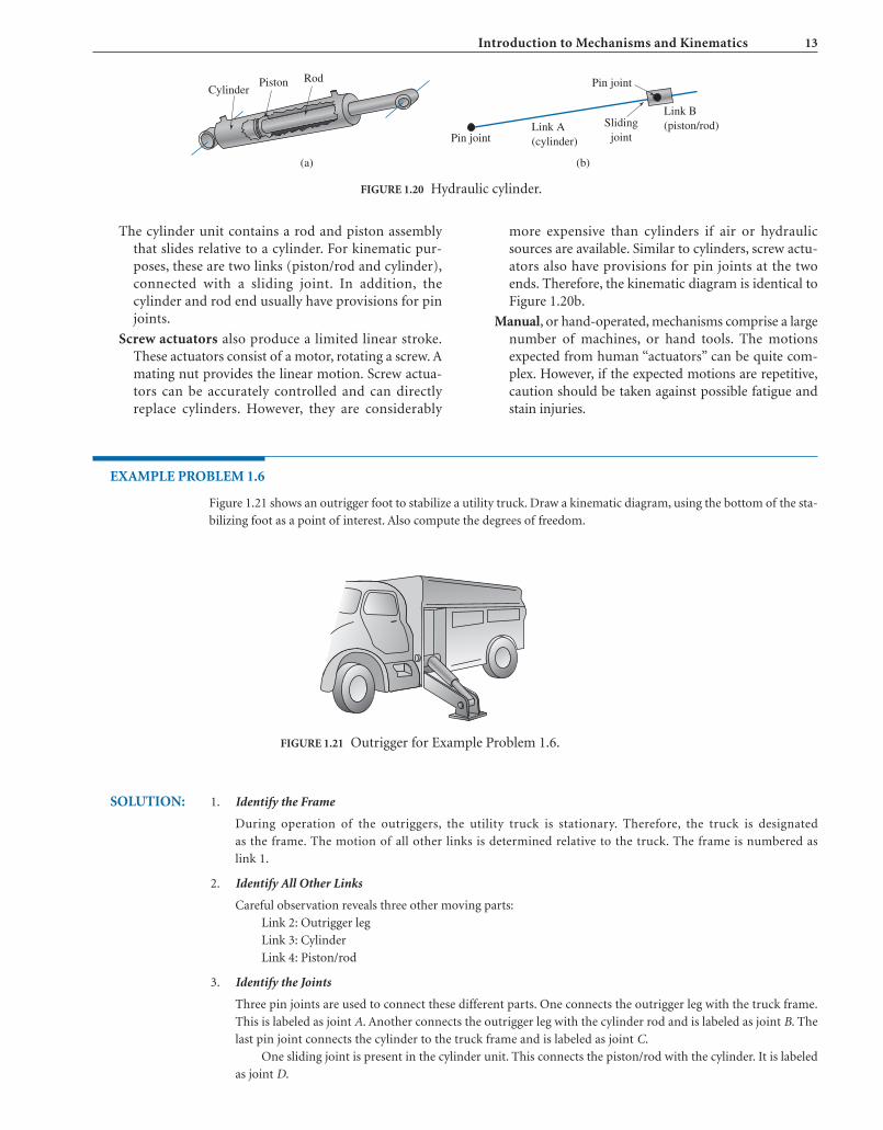
EXAMPLE PROBLEM 1.6
Figure 1.21 shows an outrigger foot to stabilize a utility truck. Draw a kinematic diagram, using the bottom of the sta-
bilizing foot as a point of interest. Also compute the degrees of freedom.
SOLUTION: 1. Identify the Frame
During operation of the outriggers, the utility truck is stationary. Therefore, the truck is designated
as the frame. The motion of all other links is determined relative to the truck. The frame is numbered as
link 1.
2. Identify All Other Links
Careful observation reveals three other moving parts:
Link 2: Outrigger leg
Link 3: Cylinder
Link 4: Piston/rod
3. Identify the Joints
Three pin joints are used to connect these different parts. One connects the outrigger leg with the truck frame.
This is labeled as joint A. Another connects the outrigger leg with the cylinder rod and is labeled as joint B. The
last pin joint connects the cylinder to the truck frame and is labeled as joint C.
One sliding joint is present in the cylinder unit. This connects the piston/rod with the cylinder. It is labeled
as joint D.

14 CHAPTER ONE
(b) Eccentric crank(a) Eccentric crankshaft
e
e
(c) Eccentric crank model
e
C
BD
X
A
2
4
31
FIGURE 1.22 Kinematic diagram for Example Problem 1.6.
FIGURE 1.23 Eccentric crank.
4. Identify Any Points of Interest
The stabilizer foot is part of link 2, and a point of interest located on the bottom of the foot is labeled as point of
interest X.
5. Draw the Kinematic Diagram
The resulting kinematic diagram is given in Figure 1.22.
6. Calculate Mobility
To calculate the mobility, it was determined that there are four links in this mechanism, as well as three pin joints
and one slider joint. Therefore,
and
With one degree of freedom, the outrigger mechanism is constrained. Moving only one link, the piston,
precisely positions all other links in the outrigger, placing the stabilizing foot on the ground.
M = 3(n - 1) - 2jp - jh = 3(4 - 1) - 2(4) - 0 = 1
n = 4, jp = (3 pins + 1 slider) = 4, jh = 0
1.8 COMMONLY USED LINKS AND JOINTS
1.8.1 Eccentric Crank
On many mechanisms, the required length of a crank is soshort that it is not feasible to fit suitably sized bearings at thetwo pin joints. A common solution is to design the link as aneccentric crankshaft, as shown in Figure 1.23a. This is thedesign used in most engines and compressors.
The pin, on the moving end of the link, is enlargedsuch that it contains the entire link. The outside circumfer-ence of the circular lobe on the crankshaft becomes themoving pin joint, as shown in Figure 1.23b. The location ofthe fixed bearing, or bearings, is offset from the eccentriclobe. This eccentricity of the crankshaft, , is the effectivelength of the crank. Figure 1.23c illustrates a kinematic
e
model of the eccentric crank. The advantage of the eccen-tric crank is the large surface area of the moving pin, whichreduces wear.
1.8.2 Pin-in-a-Slot Joint
A common connection between links is a pin-in-a-slotjoint, as shown in Figure 1.24a. This is a higher-order jointbecause it permits the two links to rotate and slide relativeto each other. To simplify the kinematic analysis, primaryjoints can be used to model this higher-order joint. Thepin-in-a-slot joint becomes a combination of a pin jointand a sliding joint, as in Figure 1.24b. Note that thisinvolves adding an extra link to the mechanism. In bothcases, the relative motion between the links is the same.However, using a kinematic model with primary jointsfacilitates the analysis.

Introduction to Mechanisms and Kinematics 15
(b) Pin-in-a-slot model(a) Actual pin-in-a-slot joint
(b) Screw modeled as a slider(a) Actual screw joint
FIGURE 1.26 Lift table for Example Problem 1.7.
FIGURE 1.24 Pin-in-a-slot joint.
FIGURE 1.25 Screw joint.
1.8.3 Screw Joint
A screw joint, as shown in Figure 1.25a, is another commonconnection between links. Screw mechanisms are discussedin detail in Chapter 12. To start with, a screw joint permitstwo relative, but dependent, motions between the links beingjoined. A specific rotation of one link will cause an associ-ated relative translation between the two links. For example,turning the screw one revolution may move the nut alongthe screw threads a distance of 0.1 in. Thus, only one inde-pendent motion is introduced.
A screw joint is typically modeled with a sliding joint, asshown in Figure 1.25b. It must be understood that out-of-plane rotation occurs. However, only the relative translationbetween the screw and nut is considered in planar kinematicanalysis.
An actuator, such as a hand crank, typically producesthe out-of-plane rotation. A certain amount of rotation willcause a corresponding relative translation between the linksbeing joined by the screw joint. This relative translation isused as the “driver” in subsequent kinematic analyses.
EXAMPLE PROBLEM 1.7
Figure 1.26 presents a lift table used to adjust the working height of different objects. Draw a kinematic diagram and
compute the degrees of freedom.
SOLUTION: 1. Identify the Frame
The bottom base plate rests on a fixed surface. Thus, the base plate will be designated as the frame. The bearing
at the bottom right of Figure 1.26 is bolted to the base plate. Likewise, the two bearings that support the screw on
the left are bolted to the base plate.
From the discussion in the previous section, the out-of-plane rotation of the screw will not be considered.
Only the relative translation of the nut will be included in the kinematic model. Therefore, the screw will also
be considered as part of the frame. The motion of all other links will be determined relative to this bottom base
plate, which will be numbered as link 1.

16 CHAPTER ONE
(b) Two rotating and one sliding link(a) Three rotating links
FIGURE 1.28 Three links connected at a common pin joint.
2 A
5
6
3 4
1
C D
E
B
FIGURE 1.27 Kinematic diagram for Example Problem 1.7.
2. Identify All Other Links
Careful observation reveals five other moving parts:
Link 2: Nut
Link 3: Support arm that ties the nut to the table
Link 4: Support arm that ties the fixed bearing to the slot in the table
Link 5: Table
Link 6: Extra link used to model the pin in slot joint with separate pin and slider joints
3. Identify the Joints
A sliding joint is used to model the motion between the screw and the nut. A pin joint, designated as point A,
connects the nut to the support arm identified as link 3. A pin joint, designated as point B, connects the two sup-
port arms––link 3 and link 4. Another pin joint, designated as point C, connects link 3 to link 6. A sliding joint
joins link 6 to the table, link 5. A pin, designated as point D, connects the table to the support arm, link 3. Lastly,
a pin joint, designated as point E, is used to connect the base to the support arm, link 4.
4. Draw the Kinematic Diagram
The kinematic diagram is given in Figure 1.27.
5. Calculate Mobility
To calculate the mobility, it was determined that there are six links in this mechanism. There are also five pin
joints and two slider joints. Therefore
and
With one degree of freedom, the lift table has constrained motion. Moving one link, the handle that rotates
the screw, will precisely position all other links in the device, raising or lowering the table.
M = 3(n - 1) - 2jp - j h = 3(6 - 1) - 2(7) - 0 = 15 - 14 = 1
n = 6 jp = (5 pins + 2 sliders) = 7 j h = 0
1.9 SPECIAL CASES OF THE MOBILITYEQUATION
Mobility is an extremely important property of a mecha-nism. Among other facets, it gives insight into the number ofactuators required to operate a mechanism. However, toobtain correct results, special care must be taken in using theGruebler’s equation. Some special conditions are presentednext.
1.9.1 Coincident Joints
Some mechanisms have three links that are all connected at acommon pin joint, as shown in Figure 1.28. This situationbrings some confusion to kinematic modeling. Physically,
one pin may be used to connect all three links. However, bydefinition, a pin joint connects two links.
For kinematic analysis, this configuration must be mathe-matically modeled as two separate joints. One joint will
Introduction to Mechanisms and Kinematics 17
FIGURE 1.29 Mechanical press for Example Problem 1.8.
connect the first and second links. The second joint will thenconnect the second and third links. Therefore, when three links
come together at a common pin, the joint must be modeled astwo pins. This scenario is illustrated in Example Problem 1.8.
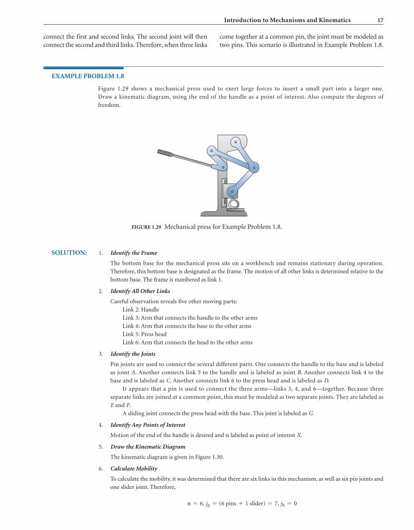
EXAMPLE PROBLEM 1.8
Figure 1.29 shows a mechanical press used to exert large forces to insert a small part into a larger one.
Draw a kinematic diagram, using the end of the handle as a point of interest. Also compute the degrees of
freedom.
SOLUTION: 1. Identify the Frame
The bottom base for the mechanical press sits on a workbench and remains stationary during operation.
Therefore, this bottom base is designated as the frame. The motion of all other links is determined relative to the
bottom base. The frame is numbered as link 1.
2. Identify All Other Links
Careful observation reveals five other moving parts:
Link 2: Handle
Link 3: Arm that connects the handle to the other arms
Link 4: Arm that connects the base to the other arms
Link 5: Press head
Link 6: Arm that connects the head to the other arms
3. Identify the Joints
Pin joints are used to connect the several different parts. One connects the handle to the base and is labeled
as joint A. Another connects link 3 to the handle and is labeled as joint B. Another connects link 4 to the
base and is labeled as C. Another connects link 6 to the press head and is labeled as D.
It appears that a pin is used to connect the three arms—links 3, 4, and 6—together. Because three
separate links are joined at a common point, this must be modeled as two separate joints. They are labeled as
E and F.
A sliding joint connects the press head with the base. This joint is labeled as G.
4. Identify Any Points of Interest
Motion of the end of the handle is desired and is labeled as point of interest X.
5. Draw the Kinematic Diagram
The kinematic diagram is given in Figure 1.30.
6. Calculate Mobility
To calculate the mobility, it was determined that there are six links in this mechanism, as well as six pin joints and
one slider joint. Therefore,
n = 6, jp = (6 pins + 1 slider) = 7, jh = 0

18 CHAPTER ONE
FIGURE 1.32 A cam with a roller follower.
C
E, F
XB
A
G
D
1
5 6
43
2
FIGURE 1.30 Kinematic diagram for Example Problem 1.8.
FIGURE 1.31 Mechanism that violates the Gruebler’s equation.
and
With one degree of freedom, the mechanical press mechanism is constrained. Moving only one link,
the handle, precisely positions all other links in the press, sliding the press head onto the work piece.
M = 3(n - 1) - 2jp - j h = 3(6 - 1) - 2(7) - 0 = 15 - 14 = 1
1.9.2 Exceptions to the Gruebler’sEquation
Another special mobility situation must be mentioned.Because the Gruebler’s equation does not account for linkgeometry, in rare instances it can lead to misleading results.One such instance is shown in Figure 1.31.
redundant, and because it is identical in length to the othertwo links attached to the frame, it does not alter the action ofthe linkage.
There are other examples of mechanisms that violatethe Gruebler’s equation because of unique geometry. Adesigner must be aware that the mobility equation can, attimes, lead to inconsistencies.
1.9.3 Idle Degrees of Freedom
In some mechanisms, links exhibit motion which does notinfluence the input and output relationship of the mecha-nism. These idle degrees of freedom present another situa-tion where Gruebler’s equation gives misleading results.An example is a cam with a roller follower as shown inFigure 1.32. Gruebler’s equation specifies two degrees offreedom (4 links, 3 pins, 1 higher-order joint). With anactuated cam rotation, the pivoted link oscillates while theroller follower rotates about its center. Yet, only the motionof the pivoted link serves as the output of the mechanism.
The roller rotation is an idle degree of freedom and notintended to affect the output motion of the mechanism.It is a design feature which reduces friction and wear on thesurface of the cam. While Gruebler’s equation specifies thata cam mechanism with a roller follower has a mobility oftwo, the designer is typically only interested in a singledegree of freedom. Several other mechanisms containsimilar idle degrees of freedom.
Notice that this linkage contains five links and six pinjoints. Using Gruebler’s equation, this linkage has zerodegrees of freedom. Of course, this suggests that the mecha-nism is locked. However, if all pivoted links were the samesize, and the distance between the joints on the frame andcoupler were identical, this mechanism would be capable ofmotion, with one degree of freedom. The center link is

Introduction to Mechanisms and Kinematics 19
X
(a) (b)
2
314
FIGURE 1.33 Rear-window wiper mechanism.
1.10 THE FOUR-BAR MECHANISM
The simplest and most common linkage is the four-barlinkage. It is a combination of four links, one being desig-nated as the frame and connected by four pin joints.
Because it is encountered so often, further exploration isin order.
The mechanism for an automotive rear-window wipersystem is shown in Figure 1.33a. The kinematic diagram isshown in Figure 1.33b. Notice that this is a four-bar mechanism
because it is comprised of four links connected by four pinjoints and one link is unable to move.
The mobility of a four-bar mechanism consists of thefollowing:
and
Because the four-bar mechanism has one degree offreedom, it is constrained or fully operated with one driver.The wiper system in Figure 1.33 is activated by a single DCelectric motor.
Of course, the link that is unable to move is referredto as the frame. Typically, the pivoted link that is con-nected to the driver or power source is called the inputlink. The other pivoted link that is attached to the frame isdesignated the output link or follower. The coupler orconnecting arm “couples” the motion of the input link tothe output link.
1.10.1 Grashof ’s Criterion
The following nomenclature is used to describe the length ofthe four links.
M = 3(n - 1) - 2jp - jh = 3(4 - 1) - 2(4) - 0 = 1
n = 4, jp = 4 pins, jh = 0 Grashof ’s theorem states that a four-bar mechanism has atleast one revolving link if:
Conversely, the three nonfixed links will merely rock if:
All four-bar mechanisms fall into one of the five categorieslisted in Table 1.2.
s + l 7 p + q
s + l … p + q
q = length of the other intermediate length links
p = length of one of the intermediate length links
l = length of the longest link
s = length of the shortest link
TABLE 1.2 Categories of Four-Bar Mechanisms
Case Criteria Shortest Link Category
1 s + l 6 p + q Frame Double crank
2 s + l 6 p + q Side Crank-rocker
3 s + l 6 p + q Coupler Double rocker
4 s + l = p + q Any Change point
5 s + l 7 p + q Any Triple rocker

20 CHAPTER ONE
(a) Double crank
(c) Double rocker
(d) Change point(e) Triple rocker
(b) Crank-rocker
FIGURE 1.34 Categories of four-bar mechanisms.
The different categories are illustrated in Figure 1.34and described in the following sections.
1.10.2 Double Crank
A double crank, or crank-crank, is shown in Figure 1.34a. Asspecified in the criteria of Case 1 of Table 1.2, it has the shortestlink of the four-bar mechanism configured as the frame. If oneof the pivoted links is rotated continuously, the other pivotedlink will also rotate continuously. Thus, the two pivoted links, 2and 4, are both able to rotate through a full revolution. Thedouble crank mechanism is also called a drag link mechanism.
1.10.3 Crank-Rocker
A crank-rocker is shown in Figure 1.34b. As specified in thecriteria of Case 2 of Table 1.2, it has the shortest link of thefour-bar mechanism configured adjacent to the frame. If thisshortest link is continuously rotated, the output link willoscillate between limits. Thus, the shortest link is called thecrank, and the output link is called the rocker. The wiper systemin Figure 1.33 is designed to be a crank-rocker. As the motorcontinuously rotates the input link, the output link oscillates,or “rocks.” The wiper arm and blade are firmly attached to theoutput link, oscillating the wiper across a windshield.
1.10.4 Double Rocker
The double rocker, or rocker-rocker, is shown in Figure1.34c. As specified in the criteria of Case 3 of Table 1.2, it
has the link opposite the shortest link of the four-bar mech-anism configured as the frame. In this configuration,neither link connected to the frame will be able to completea full revolution. Thus, both input and output links are con-strained to oscillate between limits, and are called rockers.However, the coupler is able to complete a full revolution.
1.10.5 Change Point Mechanism
A change point mechanism is shown in Figure 1.34d. Asspecified in the criteria of Case 4 of Table 1.2, the sum of twosides is the same as the sum of the other two. Having thisequality, the change point mechanism can be positionedsuch that all the links become collinear. The most familiartype of change point mechanism is a parallelogram linkage.The frame and coupler are the same length, and so are thetwo pivoting links. Thus, the four links will overlap eachother. In that collinear configuration, the motion becomesindeterminate. The motion may remain in a parallelogramarrangement, or cross into an antiparallelogram, or butter-fly, arrangement. For this reason, the change point is called asingularity configuration.
1.10.6 Triple Rocker
A triple rocker linkage is shown in Figure 1.34e. Exhibitingthe criteria in Case 5 of Table 1.2, the triple rocker has nolinks that are able to complete a full revolution. Thus, allthree moving links rock.
EXAMPLE PROBLEM 1.9
A nosewheel assembly for a small aircraft is shown in Figure 1.35. Classify the motion of this four-bar mechanism
based on the configuration of the links.

Introduction to Mechanisms and Kinematics 21
26"
30"
30"
32"15°
12"5"
FIGURE 1.35 Nosewheel assembly for Example Problem 1.9.
X
C
B
AD
3
2
1
4
FIGURE 1.36 Kinematic diagram for Example Problem 1.9.
SOLUTION: 1. Distinguish the Links Based on Length
In an analysis that focuses on the landing gear, the motion of the wheel assembly would be determined relative
to the body of the aircraft. Therefore, the aircraft body will be designated as the frame. Figure 1.36 shows the
kinematic diagram for the wheel assembly, numbering and labeling the links. The tip of the wheel was desig-
nated as point of interest X.
The lengths of the links are:
2. Compare to Criteria
The shortest link is a side, or adjacent to the frame. According to the criteria in Table 1.2, this mechanism can be ei-
ther a crank-rocker, change point, or a triple rocker. The criteria for the different categories of four-bar mechanisms
should be reviewed.
3. Check the Crank-Rocker (Case 2) Criteria
Is:
Because the criteria for a crank-rocker are valid, the nosewheel assembly is a crank-rocker mechanism.
44 6 56 : {yes}
(12 + 32) 6 (30 + 26)
s + l 6 p + q
s = 12 in.; l = 32 in.; p = 30 in.; q = 26 in.

22 CHAPTER ONE
A
B
(a) (b)
X
CD
1
2
3
4
FIGURE 1.37 Pump mechanism for a manual water pump: (a) Mechanism and (b) Kinematic diagram.
(a) (b)
FIGURE 1.38 Straight-line mechanisms
1.11 SLIDER-CRANK MECHANISM
Another mechanism that is commonly encountered is aslider-crank. This mechanism also consists of a combinationof four links, with one being designated as the frame. This
mechanism, however, is connected by three pin joints andone sliding joint.
A mechanism that drives a manual water pump isshown in Figure 1.37a. The corresponding kinematic dia-gram is given in Figure 1.37b.
The mobility of a slider-crank mechanism is repre-sented by the following:
and
Because the slider-crank mechanism has one degree offreedom, it is constrained or fully operated with one driver.The pump in Figure 1.37 is activated manually by pushingon the handle (link 3).
In general, the pivoted link connected to the frame iscalled the crank. This link is not always capable of complet-ing a full revolution. The link that translates is called theslider. This link is the piston/rod of the pump in Figure 1.37.
M = 3(n - 1) - 2jp - jh = 3(4 - 1) - 2(4) - 0 = 1.
n = 4, jp = (3 pins + 1 sliding) = 4, jh = 0
The coupler or connecting rod “couples” the motion of thecrank to the slider.
1.12 SPECIAL PURPOSE MECHANISMS
1.12.1 Straight-Line Mechanisms
Straight-line mechanisms cause a point to travel in a straightline without being guided by a flat surface. Historically, qual-ity prismatic joints that permit straight, smooth motionwithout backlash have been difficult to manufacture. Severalmechanisms have been conceived that create straight-line(or nearly straight-line) motion with revolute joints androtational actuation. Figure 1.38a shows a Watt linkage andFigure. 1.38b shows a Peaucellier-Lipkin linkage.
1.12.2 Parallelogram Mechanisms
Mechanisms are often comprised of links that form parallel-ograms to move an object without altering its pitch. Thesemechanisms create parallel motion for applications such as
balance scales, glider swings, and jalousie windows. Twotypes of parallelogram linkages are given in Figure 1.39awhich shows a scissor linkage and Figure1.39b which showsa drafting machine linkage.

Introduction to Mechanisms and Kinematics 23
(a) (b)
(a) (b)
FIGURE 1.39 Parallelogram mechanisms.
FIGURE 1.40 Quick-return mechanisms.
1.12.3 Quick-Return Mechanisms
Quick-return mechanisms exhibit a faster stroke in one direc-tion than the other when driven at constant speed with a rota-tional actuator. They are commonly used on machine tools
that require a slow cutting stroke and a fast return stroke. Thekinematic diagrams of two different quick-return mechanismsare given in Figure 1.40a which shows an offset slider-cranklinkage and Figure 1.40b which shows a crank-shaper linkage.
1.12.4 Scotch Yoke Mechanism
A scotch yoke mechanism is a common mechanism thatconverts rotational motion to linear sliding motion, or viceversa. As shown in Figure 1.41, a pin on a rotating link isengaged in the slot of a sliding yoke. With regards to the
input and output motion, the scotch yoke is similar to aslider-crank, but the linear sliding motion is pure sinusoidal.In comparison to the slider-crank, the scotch yoke has theadvantage of smaller size and fewer moving parts, but canexperience rapid wear in the slot.
1.13 TECHNIQUES OF MECHANISMANALYSIS
Most of the analysis of mechanisms involves geometry. Often,graphical methods are employed so that the motion of themechanism can be clearly visualized. Graphical solutions
involve drawing “scaled” lines at specific angles. One exampleis the drawing of a kinematic diagram. A graphical solutioninvolves preparing a drawing where all links are shown at aproportional scale to the actual mechanism. The orientation ofthe links must also be shown at the same angles as on the actualmechanism.
(a) Actual mechanism(a) Actual mechanism (b) Kinematic diagram
FIGURE 1.41 Scotch yoke mechanism.

24 CHAPTER ONE
This graphical approach has the merits of ease and solu-tion visualization. However, accuracy must be a serious con-cern to achieve results that are consistent with analyticaltechniques. For several decades, mechanism analysis was pri-marily completed using graphical approaches. Despite itspopularity, many scorned graphical techniques as beingimprecise. However, the development of computer-aideddesign (CAD) systems has allowed the graphical approach tobe applied with precision. This text attempts to illustrate themost common methods used in the practical analysis ofmechanisms. Each of these methods is briefly introduced inthe following sections.
1.13.1 Traditional Drafting Techniques
Over the past decades, all graphical analysis was performedusing traditional drawing techniques. Drafting equipmentwas used to draw the needed scaled lines at specific angles.The equipment used to perform these analyses includedtriangles, parallel straight edges, compasses, protractors,and engineering scales. As mentioned, this method wasoften criticized as being imprecise. However, with properattention to detail, accurate solutions can be obtained.
It was the rapid adoption of CAD software over the pastseveral years that limited the use of traditional graphicaltechniques. Even with the lack of industrial application,many believe that traditional drafting techniques can still beused by students to illustrate the concepts behind graphicalmechanism analysis. Of course, these concepts are identicalto those used in graphical analysis using a CAD system. Butby using traditional drawing techniques, the student canconcentrate on the kinematic theories and will not be“bogged down” with learning CAD commands.
1.13.2 CAD Systems
As mentioned, graphical analysis may be performed usingtraditional drawing procedures or a CAD system, as is com-monly practiced in industry. Any one of the numerous com-mercially available CAD systems can be used for mechanismanalysis. The most common two-dimensional CAD systemis AutoCAD. Although the commands differ between CADsystems, all have the capability to draw highly accurate linesat designated lengths and angles. This is exactly the capabil-ity required for graphical mechanism analysis. Besidesincreased accuracy, another benefit of CAD is that the linesdo not need to be scaled to fit on a piece of drawing paper.On the computer, lines are drawn on “virtual” paper that isof infinite size.
Additionally, the constraint-based sketching mode insolid modeling systems, such as Inventor, SolidWorks, andProEngineer, can be extremely useful for planar kinematicanalysis. Geometric constraints, such as length, perpendicu-larity, and parallelism, need to be enforced when performingkinematic analysis. These constraints are automatically exe-cuted in the solid modeler’s sketching mode.
This text does not attempt to thoroughly discuss thesystem-specific commands used to draw the lines, but
several of the example problems are solved using a CADsystem. The main goal of this text is to instill an understand-ing of the concepts of mechanism analysis. This goal can berealized regardless of the specific CAD system incorporated.Therefore, the student should not be overly concerned withthe CAD system used for accomplishing graphical analysis.For that matter, the student should not be concernedwhether manual or computer graphics are used to learnmechanism analysis.
1.13.3 Analytical Techniques
Analytical methods can also be used to achieve preciseresults. Advanced analytical techniques often involveintense mathematical functions, which are beyond thescope of this text and of routine mechanism analysis. Inaddition, the significance of the calculations is often diffi-cult to visualize.
The analytical techniques incorporated in this text couplethe theories of geometry, trigonometry, and graphical mecha-nism analysis. This approach will achieve accurate solutions,yet the graphical theories allow the solutions to be visualized.This approach does have the pitfall of laborious calculationsfor more complex mechanisms. Still, a significant portion ofthis text is dedicated to these analytical techniques.
1.13.4 Computer Methods
As more accurate analytical solutions are desired for severalpositions of a mechanism, the number of calculations canbecome unwieldy. In these situations, the use of computersolutions is appropriate. Computer solutions are also valu-able when several design iterations must be analyzed.
A computer approach to mechanism analysis can takeseveral forms:
� Spreadsheets are very popular for routine mechanismproblems. An important feature of the spreadsheet is thatas a cell containing input data is changed, all other resultsare updated. This allows design iterations to be completedwith ease. As problems become more complex, they can bedifficult to manage on a spreadsheet. Nonetheless, spread-sheets are used in problem solution throughout the text.
� Commercially available dynamic analysis programs, suchas Working Model, ADAMS (Automatic DynamicAnalysis of Mechanical Systems), or Dynamic Designer,are available. Dynamic models of systems can be createdfrom menus of general components. Limited versions ofdynamic analysis programs are solid modeling systems.Full software packages are available and best suitedwhen kinematic and dynamic analysis is a large compo-nent of the job. Chapter 2 is dedicated to dynamicanalysis programs.
� User-written computer programs in a high-level language,such as Matlab, Mathematica, VisualBasic, or , canbe created. The programming language selected musthave direct availability to trigonometric and inverse
C+ +

Introduction to Mechanisms and Kinematics 25
FIGURE P1.3 Problems 3 and 28.
FIGURE P1.1 Problems 1 and 26.
FIGURE P1.2 Problems 2 and 27.
FIGURE P1.4 Problems 4 and 29.
FIGURE P1.5 Problems 5 and 30.
FIGURE P1.6 Problems 6 and 31.
Frameattachment
Windowsupport
FIGURE P1.7 Problems 7 and 32.
trigonometric functions. Due to the time and effortrequired to write special programs, they are most effec-tive when a complex, yet not commonly encountered,problem needs to be solved. Some simple algorithms areprovided for elementary kinematic analysis in Chapter 8.
PROBLEMS
Problems in Sketching Kinematic Diagrams
1–1. A mechanism is used to open the door of a heat-treating furnace and is shown in Figure P1.1. Draw akinematic diagram of the mechanism. The end ofthe handle should be identified as a point of interest.
1–2. A pair of bolt cutters is shown in Figure P1.2. Drawa kinematic diagram of the mechanism, selectingthe lower handle as the frame. The end of the upperhandle and the cutting surface of the jaws should beidentified as points of interest.
1–7. A mechanism for a window is shown in Figure P1.7.Draw a kinematic diagram of the mechanism.
1–3. A folding chair that is commonly used in stadiums isshown in Figure P1.3. Draw a kinematic diagram ofthe folding mechanism.
1–4. A foot pump that can be used to fill bike tires, toys,and so forth is shown in Figure P1.4. Draw a kine-matic diagram of the pump mechanism. The footpad should be identified as a point of interest.
1–5. A pair of pliers is shown in Figure P1.5. Draw akinematic diagram of the mechanism.
1–6. Another configuration for a pair of pliers is shownin Figure P1.6. Draw a kinematic diagram of themechanism.
1–8. Another mechanism for a window is shown inFigure P1.8. Draw a kinematic diagram of themechanism.

26 CHAPTER ONE
Sill
Window
Microwaveoven carrier
Linear actuator
FIGURE P1.8 Problems 8 and 33.
FIGURE P1.9 Problems 9 and 34.
FIGURE P1.10 Problems 10 and 35.
FIGURE P1.11 Problems 11 and 36.
FIGURE P1.12 Problems 12 and 37.
FIGURE P1.13 Problems 13 and 38.
1–14. A sketch of a truck used to deliver supplies to passen-ger jets is shown in Figure P1.14. Draw a kinematicdiagram of the mechanism.
1–9. A toggle clamp used for holding a work piece whileit is being machined is shown in Figure P1.9. Draw akinematic diagram of the mechanism.
1–10. A child’s digging toy that is common at manymunicipal sandboxes is shown in Figure P1.10. Draw akinematic diagram of the mechanism.
1–11. A reciprocating saw, or saws all, is shown inFigure P1.11. Draw a kinematic diagram of themechanism that produces the reciprocatingmotion.
1–12. A small front loader is shown in Figure P1.12. Drawa kinematic diagram of the mechanism.
1–13. A sketch of a microwave oven carrier used to assistpeople in wheelchairs is shown in Figure P1.13.Draw a kinematic diagram of the mechanism.

Introduction to Mechanisms and Kinematics 27
FIGURE P1.14 Problems 14 and 39.
FIGURE P1.16 Problems 16 and 41.
FIGURE P1.15 Problems 15 and 40.
FIGURE P1.17 Problems 17 and 42.
FIGURE P1.18 Problems 18 and 43.
FIGURE P1.19 Problems 19 and 44.
FIGURE P1.20 Problems 20 and 45.
1–21. A sketch of a kitchen appliance carrier, used forundercounter storage, is shown in Figure P1.21.Draw a kinematic diagram of the mechanism.
1–15. A sketch of a device to move packages from an assem-bly bench to a conveyor is shown in Figure P1.15.Draw a kinematic diagram of the mechanism.
1–16. A sketch of a lift platform is shown in Figure P1.16.Draw a kinematic diagram of the mechanism.
1–17. A sketch of a lift platform is shown in Figure P1.17.Draw a kinematic diagram of the mechanism.
1–18. A sketch of a backhoe is shown in Figure P1.18.Draw a kinematic diagram of the mechanism.
1–19. A sketch of a front loader is shown in Figure P1.19.Draw a kinematic diagram of the mechanism.
1–20. A sketch of an adjustable-height platform usedto load and unload freight trucks is shown inFigure P1.20. Draw a kinematic diagram of themechanism.

28 CHAPTER ONE
FIGURE P1.24 Problems 24 and 49.
Testspecimen
FIGURE P1.22 Problems 22 and 47.
FIGURE P1.23 Problems 23 and 48. FIGURE P1.25 Problems 25 and 50.
1–23. A sketch of a device to close the top flaps of boxes isshown in Figure P1.23. Draw a kinematic diagramof the mechanism.
1–24. A sketch of a sewing machine is shown in Figure P1.24.Draw a kinematic diagram of the mechanism.
Counter
Microwaveoven
FIGURE P1.21 Problems 21 and 46.
1–22. An automotive power window mechanism is shownin Figure P1.22. Draw a kinematic diagram of themechanism.
1–25. A sketch of a wear test fixture is shown in Figure P1.25.Draw a kinematic diagram of the mechanism.

Introduction to Mechanisms and Kinematics 29
b
c
d
a
DC
B A
FIGURE P1.51 Problems 51 to 54.
FIGURE C1.1 (Courtesy Industrial Press, Inc.).
Problems in Calculating MobilitySpecify the number of links and the number of joints and calculatethe mobility for the mechanism shown in the figure.
1–26. Use Figure P1.11–27. Use Figure P1.21–28. Use Figure P1.31–29. Use Figure P1.41–30. Use Figure P1.51–31. Use Figure P1.61–32. Use Figure P1.71–33. Use Figure P1.81–34. Use Figure P1.91–35. Use Figure P1.101–36. Use Figure P1.111–37. Use Figure P1.121–38. Use Figure P1.131–39. Use Figure P1.141–40. Use Figure P1.151–41. Use Figure P1.161–42. Use Figure P1.171–43. Use Figure P1.181–44. Use Figure P1.191–45. Use Figure P1.201–46. Use Figure P1.211–47. Use Figure P1.221–48. Use Figure P1.231–49. Use Figure P1.241–50. Use Figure P1.25
Problems in Classifying Four-Bar
Mechanisms
1–51. A mechanism to spray water onto vehicles at anautomated car wash is shown in Figure P1.51.
1. As link A rotates clockwise 90°, what will happen toslide C?
2. What happens to the ball trapped in slide C when itis at this position?
3. As link A continues another 90° clockwise, whataction occurs?
4. What is the purpose of this device?5. Why are there chamfers at the entry of slide C?6. Why do you suppose there is a need for such a
device?
1–2. Figure C1.2 shows a mechanism that is typical in thetank of a water closet. Note that flapper C is hollowand filled with trapped air. Carefully examine theconfiguration of the components in the mechanism.Then answer the following leading questions to gaininsight into the operation of the mechanism.
1. As the handle A is rotated counterclockwise, what isthe motion of flapper C?
2. When flapper C is raised, what effect is seen?3. When flapper C is lifted, it tends to remain in an
upward position for a period of time. What causesthis tendency to keep the flapper lifted?
4. When will this tendency (to keep flapper C lifted)cease?
Classify the four-bar mechanism, based on its possi-ble motion, when the lengths of the links are
, , , and
1–52. For the water spray mechanism in Figure P1.51, clas-sify the four-bar mechanism, based on its possible
d = 4 in.c = 14 in.b = 1.5 in.a = 12 in.
motion, when the lengths of the links are ,, , and
1–53. For the water spray mechanism in Figure P1.51, clas-sify the four-bar mechanism, based on its possiblemotion, when the lengths of the links are ,
, , and
1–54. For the water spray mechanism in Figure P1.51, clas-sify the four-bar mechanism, based on its possiblemotion, when the lengths of the links are ,
, , and
CASE STUDIES
1–1. The mechanism shown in Figure C1.1 has beentaken from a feed device for an automated ball bear-ing assembly machine. An electric motor is attachedto link A as shown. Carefully examine the configura-tion of the components in the mechanism. Thenanswer the following leading questions to gaininsight into the operation of the mechanism.
d = 5 in.c = 12 in.b = 3 in.a = 12 in.
d = 4 in.c = 8 in.b = 3 in.a = 12 in.
d = 4 in.c = 12 in.b = 5 in.a = 12 in.

30 CHAPTER ONE
Watersupply
B2
B1
S R
C
FIGURE C1.3 (Courtesy Industrial Press, Inc.).
5. What effect will cause item D to move?6. As item D is moved in a counterclockwise direction,
what happens to item F?7. What does item F control?8. What is the overall operation of these mechanisms?9. Why is there a need for this mechanism and a need
to store water in this tank?
1–3. Figure C1.3 shows a mechanism that guides newlyformed steel rods to a device that rolls theminto reels. The rods are hot when formed, andwater is used to assist in the cooling process. Therods can be up to several thousand feet long andslide at rates up to 25 miles per hour throughchannel S.
Once the reel is full, the reel with the coiled rod is thenremoved. In order to obtain high efficiency, the rods followone another very closely. It is impossible to remove the reel
in a short time interval; therefore, it is desirable to use tworeels in alternation. This mechanism has been designed tofeed the rods to the reels.
Buckets B1 and B2 have holes in the bottom. The waterflow from the supply is greater than the amount that canescape from the holes. Carefully examine the configurationof the components in the mechanism, then answer the fol-lowing leading questions to gain insight into the operationof the mechanism.
1. In the shown configuration, what is happening tothe level of water in bucket B1?
2. In the shown configuration, what is happening tothe level of water in bucket B2?
3. What would happen to rocker arm C if bucket B2
were forced upward?4. What would happen to rocker arm R if bucket B2
were forced upward?5. What does rocker arm R control?6. What is the continual motion of this device?7. How does this device allow two separate reels to be
used for the situation described?8. Why do you suppose that water is used as the power
source for the operation of this mechanism?
F
C
AD
FIGURE C1.2 (Courtesy Industrial Press, Inc.).

2.2 COMPUTER SIMULATIONOF MECHANISMS
Along with Working Model®, other dynamic analysisprograms are available. These include ADAMS® (AutomaticDynamic Analysis of Mechanical Systems), DynamicDesigner®, LMS Virtual.Lab, and Analytix®. All these com-puter programs allow creation of a mechanism from menus,or icons, of general components. The general componentsinclude those presented in Chapter 1, such as simple links,complex links, pin joints, sliding joints, and gear joints. Themechanism is operated by selecting actuator components,such as motors or cylinders, from menus.
In machine design, one of the reasons for the widespreadadoption of solid modeling is that it sets the stage for manyancillary uses: Working drawings can be nearly automaticallycreated, renderings that closely resemble the real machine aregenerated, and prototypes can be readily fabricated. Manyproducts that work with the solid modeling software areavailable to analyze the structural integrity of machine com-ponents. Similarly, studying the motion and forces of movingmechanisms and assemblies is becoming almost an automaticside effect of solid modeling. Figure 2.1 illustrates a solidmodel design being analyzed with Dynamic Designer withinthe Autodesk Inventor® Environment.
Regardless of software, the general strategy for performingthe dynamic analysis can be summarized as follows:
1. Define a set of rigid bodies (sizes, weights, and inertialproperties). These could be constructed in the solidmodeling design package.
2. Place constraints on the rigid bodies (connecting therigid bodies with joints).
3. Specify the input motion (define the properties of thedriving motor, cylinder, etc.) or input forces.
4. Run the analysis.
5. Review the motion of the links and forces through themechanism.
Of course, the specific commands will vary among thedifferent packages. The following sections of this chapter willfocus on the details of mechanism analysis using WorkingModel 2D®. As with any software, knowledge is gained byexperimenting and performing other analyses beyond thetutorials. Thus, the student is encouraged to explore the soft-ware by “inventing” assorted virtual machines.
O B J E C T I V E S
Upon completion of this chapter, the student will be able to:
1. Understand the use of commercially available softwarefor mechanism analysis.
2. Use Working Model® to build kinematic models ofmechanisms.
3. Use Working Model® to animate the motion ofmechanisms.
4. Use Working Model® to determine the kinematic valuesof a mechanism.
C H A P T E R
T W O
BUILDING COMPUTER MODELSOF MECHANISMS USING WORKING MODEL® SOFTWARE
2.1 INTRODUCTION
The rapid development of computers and software hasaltered the manner in which many engineering tasks arecompleted. In the study of mechanisms, software packageshave been developed that allow a designer to constructvirtual models of a mechanism. These virtual models allowthe designer to fully simulate a machine. Simulation enablesengineers to create and test product prototypes on their owndesktop computers. Design flaws can be quickly isolated andeliminated, reducing prototyping expenses and speeding thecycle of product development.
Software packages can solve kinematic and dynamicequations, determine the motion, and force values of themechanism during operation. In addition to numericalanalysis, the software can animate the computer model ofthe mechanism, allowing visualization of the design inaction.
This chapter primarily serves as a tutorial for simulatingmachines and mechanisms using Working Model® simu-lation software. Although the kinematic values generatedduring the analysis may not be fully understood, the visual-ization of the mechanism can be extremely insightful. Thematerial presented in the next several chapters will allow thestudent to understand the numerical solutions of thedynamic software. Proficiency in this type of mechanism-analysis software, coupled with a solid understanding ofkinematic and dynamic analysis, will provide a strong basisfor machine design.
31

32 CHAPTER TWO
2.3 OBTAINING WORKING MODELSOFTWARE
Working Model 2D is created and distributed by DesignSimulation Technologies. Copies of the software can bepurchased, at substantial educational discounts, online athttp://www.workingmodel.com or http://www.design-simulation.com. A free demonstration version of WorkingModel 2D is also available for download. This demo ver-sion enables students to create fully functioning “virtualprototypes” of complex mechanical designs. However,some features are disabled, most notably the Save andPrint functions. Regardless, this version can provide anexcellent introduction to building computer models ofmechanisms. Design Simulation Technologies, Inc. can becontacted at 43311 Joy Road, #237, Canton, MI 48187,(714) 446–6935.
As Working Model 2D is updated, the menus and iconsmay appear slightly different from the tutorials in this text.However, using some intuition, the student will be able toadapt and successfully complete mechanism simulations.
2.4 USING WORKING MODEL TO MODEL A FOUR-BAR MECHANISM
As mentioned, Working Model is a popular, commerciallyavailable motion simulation package. It rapidly creates amodel on a desktop computer that represents a mechanicalsystem and performs dynamic analysis. This section usesWorking Model to build a model of a four-bar linkage andrun a simulation [Ref. 16]. It is intended to be a tutorial; thatis, it should be followed while actually using Working Model.The student is then encouraged to experiment with the soft-ware to perform other analyses.
Step 1: Open Working Model
1. Click on the Working Model program icon to start theprogram.
2. Create a new Working Model document by selecting“New” from the “File” menu.Working Model displays the user interface. Toolbars used tocreate links, joints, and mechanism actuators appear alongthe sides of the screen. Tape controls, which are used to runand view simulations, appear at the bottom of the screen.
3. Specify the units to be used in the simulation. Select“Numbers and Units” in the “View” menu. Change the“Unit System” to English (pounds).The units for linear measurements will be inches, angleswill be measured in degrees, and forces will be specified inpounds.
Step 2: Create the Links
This step creates the three moving links in a four-barmechanism. The background serves as the fixed, fourth link.
1. Construct the linkage by creating the three nonfixedlinks. Double-click on the rectangle tool on the toolbar.The tool is highlighted, indicating that it can be usedmultiple times.
2. Using the rectangle tool, sketch out three bodies asshown in Figure 2.2.Rectangles are drawn by positioning the mouse at the firstcorner, clicking once, then moving the mouse to thelocation of the opposite corner and clicking again.Rectangles are parametrically defined and their precisesizes will be specified later.
3. Open the “Properties” box and “Geometry” box in the“Window” menu.
FIGURE 2.1 Dynamic analysis of a solid model.

Building Computer Models of Mechanisms Using Working Model® Software 33
FIGURE 2.2 Three links sketched using the rectangle tool.
This displays information about the links and allowsediting of this information.
4. Use the “Properties” box to change the center of thehorizontal link to , , .The location of the rectangle should change upon dataentry.
5. Use the “Geometry” box to change the width of thehorizontal rectangle to 8.5 and the height to 0.5 in.The shape of the rectangle will change.
6. Likewise, use the “Properties” box and “Geometry” box tochange the long vertical link to be centered at ,
and have a width of 0.5 and a height of 3. Alsochange the short vertical link to be centered at ,
and have a width of 0.5 and a height of 1.5.Again, the shape and location of the rectangle shouldchange upon data entry.
7. Close both the “Properties” box and “Geometry” boxwindows.
8. The zoom icon (magnifying glass) can be used toproperly view the links.
Step 3: Place Points of Interest on the Links
This step teaches the usage of the “Object Snap” tool toplace points precisely. The “Object Snap” tool highlightscommonly used positions, like the center of a side, with an“X .” When a point is placed using “Object Snap,” thepoint’s position is automatically defined with parametricequations. These equations ensure that the point main-tains its relative location even after resizing or otheradjustments.
y = -3x = 5
y = -3x = -5
f = 0y = 0x = 0
1. Double-click on the point tool. The icon is a small circle.The point tool is highlighted, indicating that it can beused multiple times without needing to be reselected be-fore each new point is sketched.
2. Move the cursor over one of the links.Notice that an “X” appears around the pointer when it iscentered on a side, over a corner, or over the center of arectangle. This feature is called “Object Snap” and high-lights the commonly used parts of a link.
3. Place the cursor over the upper portion of one of thevertical links. When an “X ” appears around the pointer(Figure 2.3), click the mouse button.
4. Place additional points as shown in Figure 2.3.Make sure that each of these points is placed at a “snappoint” as evidenced by the “X” appearing at the pointer.
5. Select the pointer tool. The icon is an arrow pointed upand to the left.
6. Double-click on one of the points that were sketched insteps 3 or 4 to open the “Properties” window.
7. Notice that the points “snapped” to a distance of halfthe body width from the three edges. This will result ineffective link length of 8.0, 2.5, and 1.0 in.
Step 4: Connect the Points to Form Pin Joints
This step joins the points to create pin joints. A pin joint actsas a hinge between two bodies. The SmartEditor preventsjoints from breaking during a drag operation.
1. Select the anchor tool.
2. Click on the horizontal link to anchor the link down.

34 CHAPTER TWO
FIGURE 2.4 Select two points to join as a pin joint.
An anchor is used to tell the SmartEditor not to move thisbody during construction. After the pin joints have beencreated, the anchor will be deleted.
3. Select the pointer tool.
4. With the pointer tool selected, click and drag on thebackground to make a selection box that surrounds thetwo left points as shown in Figure 2.4. Release the
mouse button, and the two points should now be high-lighted (darkened).This method of selecting objects is called “box select.” Anyobject that is contained completely within the box whenthe mouse is released is highlighted.
5. Click on the “Join” button in the toolbar, merging thetwo points into a pin joint.
FIGURE 2.3 Point locations.

Building Computer Models of Mechanisms Using Working Model® Software 35
FIGURE 2.5 Adding the final pin joint and motor to the linkage.
The SmartEditor creates a pin joint between the two pointsselected, moving the unanchored link into place. The movedlink may no longer be vertical. This is fixed in a moment.
6. Perform steps 4 and 5 for the two right points to createanother pin joint.Once again, the horizontal link remains in this originalposition, and the SmartEditor moves the vertical link tocreate the pin joint.
7. Select the left vertical link by clicking on it with thepoint tool.Four black boxes appear around the link, indicating thatit has been selected. The boxes are called handles and canbe dragged to resize an object.
8. Using the coordinates bar at the bottom of the screen,enter a “0” in the (rotation) field.The coordinates fields at the bottom of the screen areuseful to obtain information on Working Model objects.These fields can also be used to edit object information.Changing the rotation to 0° adjusts the bar back to itsoriginal, vertical position.
9. If needed, complete steps 7 and 8 on the right vertical link.
10. Select the anchor used to keep the horizontal link in posi-tion during building, and press the delete key to remove it.The anchor is no longer needed and should be removed.
11. Select the “Pin Joint” tool and place a pin joint, usingthe snap point, at the lower end of the left, vertical linkas indicated in Figure 2.5. The “Pin Joint” tool appearsas two links joined by a circle.The “Pin Joint” tool is similar to the point tool used tocreate the last two pin joints. The pin tool automaticallycreates two points, attaches them to the bodies beneaththe cursor (or the body and the background, as in this
f
case), and creates a joint in one seamless step. This pinjoint joins the rectangle to the background.
12. Double-click on the pin joint to open the “Properties”window. Verify that the pin was placed half the bodywidth from the lower edge. This gives an effective linklength of 2.5 in.
Step 5: Add a Motor to the Linkage
This step adds the motor to one of the links, actuating thelinkage.
1. Click on the motor tool in the toolbox. This tool appearsas a circle, sitting on a base and with a point in its center.The motor tool becomes shaded, indicating that it has beenselected. The cursor should now look like a small motor.
2. Place the cursor over the “snap point” on the lower endof the right, vertical link. Click the mouse.A motor appears on the four-bar linkage, as shown inFigure 2.5. Similar to a pin joint, a motor has two attach-ment points. A motor automatically connects the top twobodies. If only one body were to lay beneath the motor, itwould join the body to the background. A motor wouldthen apply a torque between the two bodies to which it ispinned.
3. Double-click on the motor to open the “Properties” box.Verify that the pin was placed half the body width fromthe lower edge. This gives an effective link length of 1.0 in.
4. Specify the motor velocity to be 360 deg/s. This equatesto 60 rpm.
5. Click on “Run” in the toolbar.The four-bar linkage begins slowly cranking through itsrange of motion.
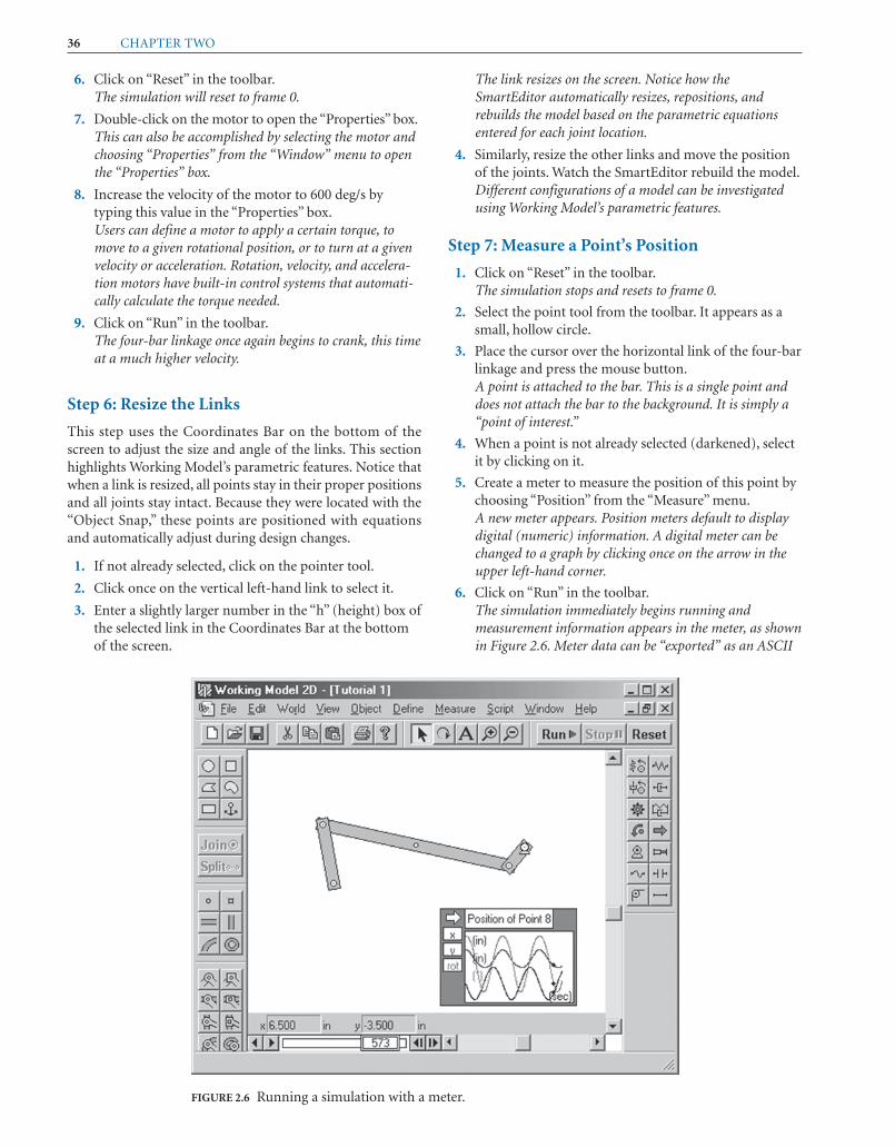
36 CHAPTER TWO
6. Click on “Reset” in the toolbar.The simulation will reset to frame 0.
7. Double-click on the motor to open the “Properties” box.This can also be accomplished by selecting the motor andchoosing “Properties” from the “Window” menu to openthe “Properties” box.
8. Increase the velocity of the motor to 600 deg/s bytyping this value in the “Properties” box.Users can define a motor to apply a certain torque, tomove to a given rotational position, or to turn at a givenvelocity or acceleration. Rotation, velocity, and accelera-tion motors have built-in control systems that automati-cally calculate the torque needed.
9. Click on “Run” in the toolbar.The four-bar linkage once again begins to crank, this timeat a much higher velocity.
Step 6: Resize the Links
This step uses the Coordinates Bar on the bottom of thescreen to adjust the size and angle of the links. This sectionhighlights Working Model’s parametric features. Notice thatwhen a link is resized, all points stay in their proper positionsand all joints stay intact. Because they were located with the“Object Snap,” these points are positioned with equationsand automatically adjust during design changes.
1. If not already selected, click on the pointer tool.
2. Click once on the vertical left-hand link to select it.
3. Enter a slightly larger number in the “h” (height) box ofthe selected link in the Coordinates Bar at the bottomof the screen.
The link resizes on the screen. Notice how theSmartEditor automatically resizes, repositions, andrebuilds the model based on the parametric equationsentered for each joint location.
4. Similarly, resize the other links and move the positionof the joints. Watch the SmartEditor rebuild the model.Different configurations of a model can be investigatedusing Working Model’s parametric features.
Step 7: Measure a Point’s Position
1. Click on “Reset” in the toolbar.The simulation stops and resets to frame 0.
2. Select the point tool from the toolbar. It appears as asmall, hollow circle.
3. Place the cursor over the horizontal link of the four-barlinkage and press the mouse button.A point is attached to the bar. This is a single point anddoes not attach the bar to the background. It is simply a“point of interest.”
4. When a point is not already selected (darkened), selectit by clicking on it.
5. Create a meter to measure the position of this point bychoosing “Position” from the “Measure” menu.A new meter appears. Position meters default to displaydigital (numeric) information. A digital meter can bechanged to a graph by clicking once on the arrow in theupper left-hand corner.
6. Click on “Run” in the toolbar.The simulation immediately begins running andmeasurement information appears in the meter, as shownin Figure 2.6. Meter data can be “exported” as an ASCII
FIGURE 2.6 Running a simulation with a meter.

Building Computer Models of Mechanisms Using Working Model® Software 37
FIGURE 2.7 Tracing the path of a point.
file, copied onto the clipboard, and pasted into aspreadsheet program for further analysis. In this case,the spreadsheet would receive four columns ofinformation: Time, X, Y, and Rotation. One row wouldappear for each integration time step calculated.
7. Modify the simulation and rerun it.Working Model’s seamless integration between theediting and running of the dynamics engine allows the user to quickly investigate many different simula-tion configurations. As an example, modify the mass of the horizontal bar using the “Properties” box,and rerun the simulation. The pin locations can bemodified and links resized; then the velocities and forces can be measured. This four-bar linkage can evenbe investigated in zero gravity by turning off gravity under the “World” menu.
Step 8: Trace the Path of a Point of Interest
This step creates a trace of the movement of a selected point.
1. Select all objects using the box select method describedearlier.All elements appear black.
2. Select the “Appearance” option in the “Window” menu.
3. In the “Appearance” window, turn off “Track Center ofMass,”“Track Connect,” and “Track Outline.”These features can be turned off by clicking over theappropriate check mark.
4. Click on the background to deselect all objects.
5. Select only the point of interest created in step 7.Only this point should appear black.
6. Select the “Appearance” option in the “Window” menu.
7. In the “Appearance” window, turn on “Track Connect.”Make sure only the one point is selected.This feature can be turned on by clicking over theappropriate check mark.
Run the simulation. The screen should look like Figure 2.7.
Step 9: Apply What has been Learned
This demonstration illustrates how to create and run simplesimulations in Working Model. The student is encouraged toexperiment with this simulation or to create an originalmechanism. Working Model has an incredible array offeatures that allows the creation of models to analyze themost complex mechanical devices.
2.5 USING WORKING MODEL TO MODEL A SLIDER-CRANKMECHANISM
This section serves as a tutorial to create a slider-crankmechanism. It should be followed while actually usingWorking Model. Again, the student is encouraged to experi-ment with the software to perform other analyses.
Step 1: Open Working Model as in Step 1 of the Previous Section
Step 2: Create the Links
This step creates the three moving links in the slider-crankmechanism. Again, the background serves as the fixed,fourth link.

38 CHAPTER TWO
FIGURE 2.8 Three links sketched using the rectangle tool.
1. Create a new Working Model document by selecting“New” from the “File” menu.
2. Specify the units to be used in the simulation. Select“Numbers and Units” in the “View” menu. Change the“Unit System” to SI (degrees).The units for linear measurement will be meters, angleswill be measured in degrees, and forces will be measuredin Newtons.
3. Construct the linkage by creating the three nonfixedlinks. Double-click on the rectangle tool in the toolbar.The tool is highlighted, indicating that it can be usedmultiple times.
4. Using the rectangle tool, sketch out three bodies asshown in Figure 2.8.Position the mouse at the first corner, click once, thenmove the mouse to the location of the opposite corner andclick again. Rectangles are parametrically defined andtheir precise sizes are specified later.
Step 3: Use the Slot Joint to Join the SlidingLink to the Background
1. Select the “keyed slot” joint icon. The icon appears as arectangle riding over a horizontal slot.
2. Move the cursor over the snap point at the center of therectangular sliding link. Click the mouse button. Thescreen should look like Figure 2.9.
3. Select the pointer tool.
4. Double-click on the slot.This opens the “Properties” window for the slot.
5. Change the angle to –45°.The incline of the slot changes.
Drag the other links until the screen appears similar toFigure 2.10.
Step 4: Connect the Other Links to Form Pin Joints
This step creates points and joins them to create pin joints. Apin joint acts as a hinge between two bodies.
1. Select the anchor tool.
2. Click on the vertical link to anchor the link down.An anchor tells the SmartEditor not to move this bodyduring construction. After the pin joints have beencreated, the anchor will be deleted.
3. Double-click on the point tool. The icon is a small circle.The point tool is highlighted, indicating that it can beused multiple times without needing to be reselectedbefore each new point is sketched.
4. Place the cursor over the upper portion of one of thevertical links. When an “X” appears around the pointer(Figure 2.11), click the mouse button.
5. Place additional points at the ends of the horizontallink, as shown in Figure 2.11.Make sure that each of these points is placed at a “snappoint” as evidenced by the “X” appearing at thepointer.
6. Place another point at the center of the sliding rectangle.This point is used to create a pin joint to the coupler.

Building Computer Models of Mechanisms Using Working Model® Software 39
FIGURE 2.9 Point and slot location.
FIGURE 2.10 Sliding joint.
7. Select the pointer tool.
8. With the pointer tool selected, click on one point thatwill be connected with a pin joint. Then, holding downthe shift key, click on the second point that will form apin joint. Notice that the two points should now behighlighted (darkened).
9. Click on the “Join” button in the toolbar, merging thetwo points into a pin joint.The SmartEditor creates a pin joint between the twoselected points, moving the unanchored link into place.The moved link may no longer be vertical. This will befixed in a moment.

40 CHAPTER TWO
FIGURE 2.12 Adding the pin joints and motor to the linkage.
FIGURE 2.11 Placing points on the other links.
10. Perform steps 8 and 9 for the other two points that willcreate another pin joint. The screen will appear similarto Figure 2.12.
Once again, the vertical link remains in this originalposition, and the SmartEditor moves the vertical link tocreate the pin joint.
11. Click on the vertical link.Four black boxes appear around the link, indicating thatit has been selected.
12. Select the “Move to front” option in the “Object” menu.This places the vertical link in front of the connectinglink, making the anchor visible.

Building Computer Models of Mechanisms Using Working Model® Software 41
13. Select the anchor, which is used to keep the vertical linkin position during building, and press the delete key toremove it.The anchor is no longer needed and should beremoved.
Step 5: Add a Motor to the Linkage
This step adds the motor to one of the links to drive the linkage.
1. Click on the motor tool in the toolbox. This toolappears as a circle, sitting on a base with a point in itscenter.The motor tool becomes shaded, indicating that it hasbeen selected. The cursor should now look like a smallmotor.
2. Place the cursor over the “snap point” on the verticallink. Click the mouse.A motor appears on the slider-crank linkage, asshown in Figure 2.12. Similar to a pin joint, a motorhas two attachment points. A motor automaticallyconnects the top two bodies. If only one body were to lay beneath the motor, the motor would join the body to the background. The motor then applies a torque between the two bodies to which it is pinned.
3. Click on “Run” in the toolbar.The slider-crank linkage begins slowly cranking throughits range of motion.
4. Click on “Reset” in the toolbar.The simulation resets to frame 0.
5. Double-click on the motor to open the “Properties”box.This can also be accomplished by selecting the motor andchoosing “Properties” from the “Window” menu to openthe “Properties” box.
6. Increase the velocity of the motor to –300 deg/s bytyping this value in the “Properties” box.Users can define a motor to apply a certain torque, tomove to a given rotational position, or to turn at a givenvelocity or acceleration. Rotation, velocity, andacceleration motors have built-in control systems thatautomatically calculate the torque needed. In this demo,we use the velocity motor.
7. Click on “Run” in the toolbar.The slider-crank linkage once again begins cranking, thistime at a much higher velocity.
Step 6: Apply What Has Been Learned
The student is encouraged to experiment with this simula-tion or to create an original mechanism. Working Modelhas an incredible array of features that allows for thecreation of a model to analyze most complex mechanicaldevices.
PROBLEMS
Use Working Model software to generate a model of a four-bar mechanism. Use the following values:
2–1. ; ; ;;
2–2. ; ; coupler =95mm ; ;
2–3. ; ; ;;
Use the Working Model software to generate a model of aslider-crank mechanism. Use the following values:
2–4. ; ; ;
2–5. ; ; coupler = 350 mm;
2–6. ; ; coupler =350 mm;
2–7. Figure P2.7 shows a mechanism that operates the land-ing gear in a small airplane. Use the Working Modelsoftware to generate a model of this linkage. The motoroperates clockwise at a constant rate of 20 rpm.
crank speed = 200 rad/scrank = 95mmoffset = 50 mm
crank speed = 200 rad/scrank = 95 mmoffset = 0mm
crank speed = 200 rad/scoupler = 4.5 in.crank = 1.45 in.offset = 0 in.
crank speed = 25 rpmfollower = 0.75 ftcoupler = 2.1 ftcrank = 0.5 ftframe = 2 ft
crank speed = 30rad/sfollower = 24mmcrank = 12 mmframe = 100mm
crank speed = 200 rad/sfollower = 3.5 in.coupler = 10 in.crank = 1 in.frame = 9 in.
26"
30"
30"
32"15°
12"
5"
FIGURE P2.7 Problem 7.
2–8. Figure P2.8 shows a mechanism that operates acoin-operated child’s amusement ride. Use theWorking Model software to generate a model of this
4" 10"
6"
27"
30"
FIGURE P2.8 Problem 8.

42 CHAPTER TWO
X
2.0 m
2.1 m.25 m
.9 m
.5 m
.6 m55°
20°
FIGURE P2.9 Problem 9.
.2 m
.2 m
.37 m
35°
.6 m
.3 m
.32 m
.65 m
.4 m.1 m.1 m
FIGURE P2.10 Problem 10.
1'
5.3'
4.5'
3.6'
6.8'
4.5'
3.5'
5.3'
3'
5.5'
FIGURE P2.11 Problem 11.
linkage. The motor operates counterclockwise at aconstant rate of 60 rpm.
2–9. Figure P2.9 shows a transfer mechanism that liftscrates from one conveyor to another. Use theWorking Model software to generate a model of thislinkage. The motor operates counterclockwise at aconstant rate of 20 rpm.
this linkage. The cylinder extends at a constant rate of1 fpm.
2–12. Figure P2.12 shows a mechanism that applies labelsto packages. Use the Working Model software togenerate a model of this linkage. The motor oper-ates counterclockwise at a constant rate of 300 rpm.
3.25"
XInk pad
Stamp
Box
8"
60°
11.25"
9.38"
6.75"
6.0"
4.32"
FIGURE P2.12 Problem 12.
G
F
Work-piece
E
C B
D
A
FIGURE C2.1 Mechanism for Case Study 2.1.
CASE STUDY
2–1. The mechanism shown in Figure C2.1 is a top viewof a fixture in a machining operation. Carefullyexamine the configuration of the components in themechanism. Then answer the following leadingquestions to gain insight into the operation of themechanism.
1. As the handle A is turned, moving the threadedrod B to the left, describe the motion of grip C.
2. As the handle A is turned, moving the threadedrod B to the left, describe the motion of grip D.
3. What is the purpose of this mechanism?4. What action would cause link D to move upward?5. What is the purpose of spring G?6. Discuss the reason for the odd shape to links E and F.7. What would you call such a device?8. Describe the rationale behind using a rounded end
for the threaded rod B.
2–10. Figure P2.10 shows another transfer mechanismthat pushes crates from one conveyor to another.Use the Working Model software to generate amodel of this linkage. The motor operates clockwiseat a constant rate of 40 rpm.
2–11. Figure P2.11 shows yet another transfer mechanismthat lowers crates from one conveyor to another. Usethe Working Model software to generate a model of

amount of donuts in the box, the amount is a scalarquantity. The following are some more examples of scalarquantities: a board is 8 ft long, a class meets for 50 min, orthe temperature is 78°F—length, time, and temperature areall scalar quantities.
In contrast, a vector is not fully defined by stating only amagnitude. Indicating the direction of the quantity is alsorequired. Stating that a golf ball traveled 200 yards does notfully describe its path. Neglecting to express the direction oftravel hides the fact that the ball has landed in a lake. Thus,the direction must be included to fully describe such a quan-tity. Examples of properly stated vectors include “the crate isbeing pulled to the right with 5 lb” or “the train is traveling ata speed of 50 mph in a northerly direction.” Displacement,force, and velocity are vector quantities.
Vectors are distinguished from scalar quantitiesthrough the use of boldface type (v). The common nota-tion used to graphically represent a vector is a linesegment having an arrowhead placed at one end. With agraphical approach to analysis, the length of the linesegment is drawn proportional to the magnitude of thequantity that the vector describes. The direction is definedby the arrowhead and the incline of the line with respect tosome reference axis. The direction is always measured atits root, not at its head. Figure 3.1 shows a fully definedvelocity vector.
O B J E C T I V E S
Upon completion of this chapter, the student will be able to:
1. Differentiate between a scalar quantity and a vector.
2. Apply the appropriate trigonometry principles toa right triangle.
3. Apply the appropriate trigonometry principles toa general triangle.
4. Determine the resultant of two vectors, using bothgraphical and analytical methods.
5. Resolve vector quantities into components in thehorizontal and vertical directions.
6. Subtract two vectors, using both graphical andanalytical methods.
7. Manipulate vector equations.
8. Utilize a vector equation to determine the magnitude of two vectors.
C H A P T E R
T H R E E
VECTORS
3.1 INTRODUCTION
Mechanism analysis involves manipulating vector quantities.Displacement, velocity, acceleration, and force are theprimary performance characteristics of a mechanism, andare all vectors. Prior to working with mechanisms, athorough introduction to vectors and vector manipulation isin order. In this chapter, both graphical and analyticalsolution techniques are presented. Students who havecompleted a mechanics course may omit this chapter or useit as a reference to review vector manipulation.
3.2 SCALARS AND VECTORS
In the analysis of mechanisms, two types of quantities needto be distinguished. A scalar is a quantity that is sufficientlydefined by simply stating a magnitude. For example, bysaying “a dozen donuts,” one describes the quantity ofdonuts in a box. Because the number “12” fully defines the
43
0
30
10 20
mph
Scale:
301 units1
2
1 unit
FIGURE 3.1 A 45 mph velocity vector.
3.3 GRAPHICAL VECTOR ANALYSIS
Much of the work involved in the study of mechanisms andanalysis of vectors involves geometry. Often, graphicalmethods are employed in such analyses because the motionof a mechanism can be clearly visualized. For more complexmechanisms, analytical calculations involving vectors alsobecome laborious.

44 CHAPTER THREE
A
Bc
a
b
C
FIGURE 3.2 The right triangle.
A graphical approach to analysis involves drawingscaled lines at specific angles. To achieve results that areconsistent with analytical techniques, accuracy must be amajor objective. For several decades, accuracy in mecha-nism analyses was obtained with attention to precision andproper drafting equipment. Even though they were popular,many scorned graphical techniques as being imprecise.However, the development of computer-aided design(CAD) with its accurate geometric constructions hasallowed graphical techniques to be applied with precision.
3.4 DRAFTING TECHNIQUES REQUIRED IN GRAPHICAL VECTOR ANALYSIS
The methods of graphical mechanism and vector analysisare identical, whether using drafting equipment or a CADpackage. Although it may be an outdated mode in industrialanalyses, drafting can be successfully employed to learn andunderstand the techniques.
For those using drafting equipment, fine lines and cir-cular arcs are required to produce accurate results. Preciselinework is needed to accurately determine intersectionpoints. Thus, care must be taken in maintaining sharp draw-ing equipment.
Accurate measurement is as important as line quality.The length of the lines must be drawn to a precise scale, andlinear measurements should be made as accurately as possi-ble. Therefore, using a proper engineering scale with inchesdivided into 50 parts is desired. Angular measurements mustbe equally precise.
Lastly, a wise choice of a drawing scale is also a veryimportant factor. Typically, the larger the construction, themore accurate the measured results are. Drawing precisionto 0.05 in. produces less error when the line is 10 in. long asopposed to 1 in. Limits in size do exist in that very largeconstructions require special equipment. However, anattempt should be made to create constructions as large aspossible.
A drawing textbook should be consulted for the detailsof general drafting techniques and geometric constructions.
3.5 CAD KNOWLEDGE REQUIRED INGRAPHICAL VECTOR ANALYSIS
As stated, the methods of graphical mechanism and vectoranalysis are identical, whether using drafting equipment or aCAD package. CAD allows for greater precision. Fortunately,only a limited level of proficiency on a CAD system isrequired to properly complete graphical vector analysis.Therefore, utilization of a CAD system is preferred andshould not require a large investment on a “learning curve.”
As mentioned, the graphical approach of vector analysisinvolves drawing lines at precise lengths and specific angles.The following list outlines the CAD abilities required forvector analysis. The user should be able to
� Draw lines at a specified length and angle;
� Insert lines, perpendicular to existing lines;
� Extend existing lines to the intersection of another line;
� Trim lines at the intersection of another line;
� Draw arcs, centered at a specified point, with a specifiedradius;
� Locate the intersection of two arcs;
� Measure the length of existing lines;
� Measure the included angle between two lines.
Of course, proficiency beyond these items facilitates moreefficient analysis. However, familiarity with CAD commandsthat accomplish these actions is sufficient to accuratelycomplete vector analysis.
3.6 TRIGONOMETRY REQUIREDIN ANALYTICAL VECTOR ANALYSIS
In the analytical analysis of vectors, knowledge of basictrigonometry concepts is required. Trigonometry is thestudy of the properties of triangles. The first type of triangleexamined is the right triangle.
3.6.1 Right Triangle
In performing vector analysis, the use of the basic trigonomet-ric functions is vitally important. The basic trigonometricfunctions apply only to right triangles. Figure 3.2 illustrates aright triangle with sides denoted as , and and interiorangles as , and . Note that angle is a 90° right angle.Therefore, the triangle is called a right triangle.
The basic trigonometric relationships are defined as:
(3.1)
(3.2)
(3.3)
These definitions can also be applied to angle :
tan ∠ B =ba
cos ∠ B =ac
sin ∠ B =bc
B
tangent∠ A = tan∠ A =side opposite
side adjacent=
a
b
cosine∠ A = cos∠ A =side adjacent
hypotenuse=
bc
sine∠ A = sin∠ A =side opposite
hypotenuse=
ac
CCA, Bca, b

Vectors 45
CA
B
35
96"
FIGURE 3.3 Front loader for Example Problem 3.1.
The Pythagorean theorem gives the relationship of thethree sides of a right triangle. For the triangle shown inFigure 3.2, it is defined as
(3.4)a2 + b2 = c2
Finally, the sum of all angles in a triangle is 180°.Knowing that angle is 90°, the sum of the other two anglesmust be
(3.5)∠A + ∠B = 90°
C
EXAMPLE PROBLEM 3.1
Figure 3.3 shows a front loader with cylinder BC in a vertical position. Use trigonometry to determine the required
length of the cylinder to orient arm AB in the configuration shown.
EXAMPLE PROBLEM 3.2
Figure 3.4 shows a tow truck with an 8-ft boom, which is inclined at a 25° angle. Use trigonometry to determine
the horizontal distance that the boom extends from the truck.
SOLUTION: 1. Determine the Horizontal Projection of the Boom
The horizontal projection of the boom can be determined from equation (3.2):
horizontal projection = (8 ft)cos 25° = 7.25 ft
cos 25° =horizontal projection
(8 ft)
SOLUTION: 1. Determine Length BC
Focus on the triangle formed by points , and Figure 3.3. The triangle side BC can be found using
equation (3.1).
solving:
2. Determine Length AC
Although not required, notice that the distance between and can similarly be determined using
equation (3.2). Thus
solving:
AC = (96 in.) cos 35° = 78.64 in.
cos 35° =AC
(96 in.)
cos ∠ A =adjacent side
hypotenuse
CA
BC = (96 in.) sin 35° = 55.06 in.
sin 35° =BC
(96 in.)
sin ∠ A =opposite side
hypotenuse
C inA, B

46 CHAPTER THREE
Overhang
8'
25
11'
6'
FIGURE 3.4 Tow truck for Example Problem 3.2.
A
BCa
b
c
FIGURE 3.5 The oblique triangle.
2. Determine Horizontal Projection of Truck and Boom
The horizontal distance from the front end of the truck to the end of the boom is
3. Determine the Overhang
Because the overall length of the truck is 11 ft, the horizontal distance that the boom extends from the
truck is
13.25 ft - 11 ft = 2.25 ft
6 ft + 7.25 ft = 13.25 ft
3.6.2 Oblique Triangle
In the previous discussion, the analysis was restricted toright triangles. An approach to general, or oblique, trianglesis also important in the study of mechanisms. Figure 3.5shows a general triangle. Again, , and denote the lengthof the sides and , , and represent the interiorangles.
For this general case, the basic trigonometric functionsdescribed in the previous section are not applicable. To ana-lyze the general triangle, the law of sines and the law ofcosines have been developed.
The law of sines can be stated as
(3.6)
The law of cosines can be stated as:
(3.7)
In addition, the sum of all interior angles in a generaltriangle must total 180°. Stated in terms of Figure 3.4 theequation would be
(3.8)∠ A + ∠ B + ∠ C = 180°
c2 = a2 + b2 - 2ab cos∠C
a
sin∠A=
b
sin ∠B=
c
sin ∠C
∠C∠B∠Aca, b
Problems involving the solution of a general triangle fallinto one of four cases:
Case 1: Given one side and two angles and .
To solve a problem of this nature, equation (3.8) can beused to find the third angle:
The law of sines can be rewritten to find the remainingsides.
Case 2: Given two sides and and the angle opposite toone of the sides .
To solve a Case 2 problem, the law of sines can be usedto find the second angle. Equation (3.6) is rewritten as
Equation (3.8) can be used to find the third angle:
The law of cosines can be used to find the third side.Equation (3.7) is rewritten as:
c = 3{a2 + b2 - 2ab cos ∠C}
∠C = 180° - ∠A - ∠B
∠B = sin -1e a bab sin ∠A f
(∠A)b)(a
c = ae sin ∠C
sin ∠Af
b = ae sin ∠B
sin ∠Af
∠C = 180° - ∠A - ∠B
∠B)(∠A(a)
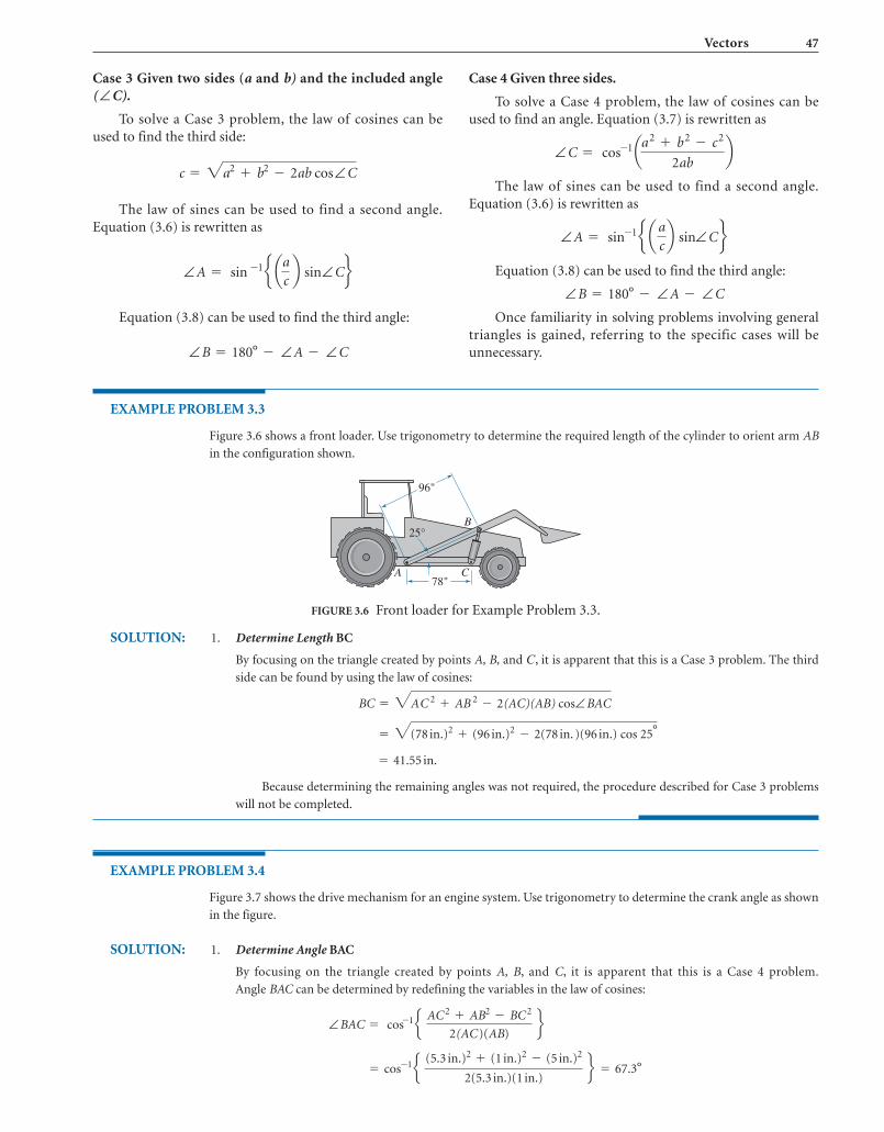
Vectors 47
A C
B
96"
25°
78"
FIGURE 3.6 Front loader for Example Problem 3.3.
Case 3 Given two sides and and the included angle.
To solve a Case 3 problem, the law of cosines can beused to find the third side:
The law of sines can be used to find a second angle.Equation (3.6) is rewritten as
Equation (3.8) can be used to find the third angle:
∠B = 180° - ∠A - ∠C
∠A = sin -1e aacb sin ∠Cf
c = 2a2 + b2 - 2ab cos ∠C
(∠C)b)(a Case 4 Given three sides.
To solve a Case 4 problem, the law of cosines can beused to find an angle. Equation (3.7) is rewritten as
The law of sines can be used to find a second angle.Equation (3.6) is rewritten as
Equation (3.8) can be used to find the third angle:
Once familiarity in solving problems involving generaltriangles is gained, referring to the specific cases will beunnecessary.
∠B = 180° - ∠A - ∠C
∠A = sin-1e aacb sin ∠C f
∠C = cos -1 aa2 + b2 - c2
2abb
EXAMPLE PROBLEM 3.3
Figure 3.6 shows a front loader. Use trigonometry to determine the required length of the cylinder to orient arm AB
in the configuration shown.
EXAMPLE PROBLEM 3.4
Figure 3.7 shows the drive mechanism for an engine system. Use trigonometry to determine the crank angle as shown
in the figure.
SOLUTION: 1. Determine Angle BAC
By focusing on the triangle created by points , and , it is apparent that this is a Case 4 problem.
Angle BAC can be determined by redefining the variables in the law of cosines:
= cos-1e (5.3 in.)2 + (1 in.)2 - (5 in.)2
2(5.3 in.)(1 in.)f = 67.3°
∠BAC = cos-1e AC 2 + AB2 - BC 2
2(AC)(AB)f
CA, B
SOLUTION: 1. Determine Length BC
By focusing on the triangle created by points A, B, and , it is apparent that this is a Case 3 problem. The third
side can be found by using the law of cosines:
Because determining the remaining angles was not required, the procedure described for Case 3 problems
will not be completed.
= 41.55 in.
= 3(78 in.)2 + (96 in.)2 - 2(78 in. )(96 in.) cos 25°
BC = 3AC 2 + AB 2 - 2(AC)(AB) cos∠BAC
C

48 CHAPTER THREE
A
B
C
5.3"
5"
Crankangle
1"
FIGURE 3.7 Engine linkage for Example Problem 3.4.
2. Determine the Crank Angle
Angle BAC is defined between side AC (the vertical side) and leg AB. Because the crank angle is defined from a
horizontal axis, the crank angle can be determined by the following:
3. Determine the Other Interior Angles
Although not required in this problem, angle ACB can be determined by
Finally, angle ABC can be found by
∠ABC = 180° - 67.3° - 10.6° = 102.1°
= sin-1e a 1 in.
5 in.b sin 67.3°f = 10.6°
∠ACB = sin-1e aAB
BCb sin∠BAC f
Crank angle = 90° - 67.3° = 22.7°
3.7 VECTOR MANIPULATION
Throughout the analysis of mechanisms, vector quantities(e.g., displacement or velocity) must be manipulated in dif-ferent ways. In a similar manner to scalar quantities, vectorscan be added and subtracted. However, unlike scalar quanti-ties, these are not simply algebraic operations. Because it isalso required to define a vector, direction must be accountedfor during mathematical operations. Vector addition andsubtraction are explored separately in the following sections.
Adding vectors is equivalent to determining the com-bined, or net, effect of two quantities as they act together.For example, in playing a round of golf, the first shot off thetee travels 200 yards but veers off to the right. A second shotthen travels 120 yards but to the left of the hole. A third shotof 70 yards places the golfer on the green. As this golferlooks on the score sheet, she notices that the hole is labeled as 310 yards; however, her ball traveled 390 yards
yards).As repeatedly stated, the direction of a vector is just as
important as the magnitude. During vector addition,does not always equal 2; it depends on the direction of theindividual vectors.
1 + 1
(200 + 120 + 70
3.8 GRAPHICAL VECTOR ADDITION
Graphical addition is an operation that determines the neteffect of vectors. A graphical approach to vector additioninvolves drawing the vectors to scale and at the properorientation. These vectors are then relocated, maintainingthe scale and orientation. The tail of the first vector isdesignated as the origin (point . The second vector isrelocated so that its tail is placed on the tip of the firstvector. The process then is repeated for all remainingvectors. This technique is known as the tip-to-tail methodof vector addition. This name is derived from viewing acompleted vector polygon. The tip of one vector runs intothe tail of the next.
The combined effect is the vector that extends fromthe tail of the first vector in the series to the tip of thelast vector in the series. Mathematically, an equationcan be written that represents the combined effect ofvectors:
R = A +7 B +7 C +7 D +7 . . .
O)
(+ 7)

Vectors 49
FIGURE 3.8 Vectors for Example Problem 3.5.
Vector R is a common notation used to represent the resultantof a series of vectors. A resultant is a term used to describe thecombined effect of vectors. Also note that the symbol isused to identify vector addition and to differentiate it fromalgebraic addition [Ref. 5].
It should be noted that vectors follow the commutativelaw of addition; that is, the order in which the vectors areadded does not alter the result. Thus,
+>The process of combining vectors can be completed graphi-cally, using either manual drawing techniques or CAD soft-ware. Whatever method is used, the underlying concepts areidentical. The following example problems illustrate thisconcept.
1B +> A +> C2 = . . .
R = 1A +> B +> C2 = 1C +> B +> A2 =
EXAMPLE PROBLEM 3.5
Graphically determine the combined effect of velocity vectors A and B, as shown in Figure 3.8.
SOLUTION: 1. Construct Vector Diagrams
To determine the resultant, the vectors must be relocated so that the tail of B is located at the tip of A. To verify
the commutative law, the vectors were redrawn so that the tail of A is placed at the tip of B. The resultant is
the vector drawn from the tail of the first vector, the origin, to the tip of the second vector. Both vector diagrams
are shown in Figure 3.9.
2. Measure the Resultant
The length vector R is measured as 66 in./s. The direction is also required to fully define vector R. The angle
from the horizontal to vector R is measured as 57°. Therefore, the proper manner of presenting the solution is
as follows:
R = 66 in./s 57°
FIGURE 3.9 The combined effect of vectors A and B for Example Problem 3.5.
0
30° 60°
25
in./s
Scale:
50
A = 59 in./s B = 30 in./s
Q

50 CHAPTER THREE
A = 200 lbB = 226 lb C = 176 lb
D = 300 lb
15° 45° 20°
0 100
lb
Scale:
200
FIGURE 3.10 Vectors for Example Problem 3.6.
SOLUTION: 1. Construct Vector Diagrams
To determine the resultant, the vectors must be relocated so that the tail of B is located at the tip of A. Then the
tail of C is placed on the tip of B. Finally, the tail of D is placed on the tip of C. Again, the ordering of vectors is
not important, and any combination could be used. As an illustration, another arbitrary combination is used in
this example. The resultant is the vector drawn from the tail of the first vector, at the origin, to the tip of the
fourth vector. The vector diagrams are shown in Figure 3.11.
2. Measure the Resultant
The length vector R is measured as 521 lb. The direction is also required to fully define the vector R. The angle
from the horizontal to vector R is measured as 68°. Therefore, the proper manner of presenting the solution is as
follows:
R = 521 in./s 68°
3.9 ANALYTICAL VECTOR ADDITION : TRIANGLE METHOD
Two analytical methods can be used to determine the neteffect of vectors. The first method is best suited when the resultant of only two vectors is required. As with the
(+ 7)graphical method, the two vectors to be combined areplaced tip-to-tail. The resultant is found by connectingthe tail of the first vector to the tip of the second vector.Thus, the resultant forms the third side of a triangle. Ingeneral, this is an oblique triangle, and the laws des-cribed in Section 3.6.2 can be applied. The length of thethird side and a reference angle must be determined
FIGURE 3.11 The combined effect of vectors A, B, C, and D for Example Problem 3.6.
EXAMPLE PROBLEM 3.6
Graphically determine the combined effect of force vectors A, B, C, and D, as shown in Figure 3.10.
Q

Vectors 51
A = 46 ft/s2
B = 23 ft/s2
20°75°
FIGURE 3.12 Vectors for Example Problem 3.7.
R
B
R = A +> B
A
75°
20°β
θ
FIGURE 3.13 Combined effect of vectors A and B forExample Problem 3.7.
EXAMPLE PROBLEM 3.7
Analytically determine the resultant of two acceleration vectors as shown in Figure 3.12.
SOLUTION: 1. Sketch a Rough Vector Diagram
The vectors are placed tip-to-tail as shown in Figure 3.13. Note that only a rough sketch is required because the
resultant is analytically determined.
2. Determine an Internal Angle
The angle between A and the horizontal is 20°. By examining Figure 3.13, the angle between vectors
A and B is:
Therefore, the problem of determining the resultant of two vectors is actually a general triangle situation as
described in Section 3.6.2 (Case 3).
3. Determine Resultant Magnitude
By following the procedure outlined for a Case 3 problem, the law of cosines is used to find the magnitude of the
resultant:
4. Determine Magnitude Direction
The law of sines can be used to find the angle between vectors A and R:
5. Fully Specify Resultant
The angle from the horizontal is . The resultant can be properly written as:
or
R = 53.19 ft./s2 134.5°
R = 53.19 ft. /s2 45.5°
20° + 25.5° = 45.5°
= sin-1e (23 ft/s2)
(53.19 ft/s2) sin 95°f = 25.5°
b = sin-1e aB
Rb sin u f
= 3(46 ft/s2)2 + (23 ft/s2)2 - 2(46 ft/s2)(23 ft/s2){cos9°} = 53.19 ft/s2
R = 2A2 + B 2 - 2ABcosu
u = 20° + 75° = 95°
through the laws of sines and cosines to fully definethe resultant vector. This method can be illustratedthrough an example problem. To clearly distinguish
quantities, vectors are shown in boldface type (D) whilethe magnitude of the vector is shown as non-bold, italictype .(D)
a
Q

52 CHAPTER THREE
3.10 COMPONENTS OF A VECTOR
The second method for analytically determining theresultant of vectors is best suited for problems where morethan two vectors are to be combined. This method involvesresolving vectors into perpendicular components.
Resolution of a vector is the reverse of combiningvectors. A single vector can be broken into two separatevectors, along convenient directions. The two vector com-ponents have the same effect as the original vector.
In most applications, it is desirable to concentrate on aset of vectors directed vertically and horizontally; therefore,a typical problem involves determining the horizontal andvertical components of a vector. This problem can be solvedby using the tip-to-tail approach, but in reverse. To explainthe method, a general vector, A, is shown in Figure 3.14.
important. Therefore, it is irrelevant whether the horizontalor vertical vector is drawn first. Figure 3.14c illustrates thecomponents of a general vector in the opposite order.
Notice that the magnitude of the components can befound from determining the sides of the triangles shown inFigure 3.14. These triangles are always right triangles, andthe methods described in Section 3.3 can be used. Thedirections of the components are taken from sketching thevectors as in Figure 3.14b or 3.14c. Standard notation con-sists of defining horizontal vectors directed toward the rightas positive. All vertical vectors directed upward are alsodefined as positive. In this fashion, the direction of thecomponents can be determined from the algebraic sign asso-ciated with the component.
An alternative method to determine the rectangularcomponents of a vector is to identify the vector’s angle withthe positive -axis of a conventional Cartesian coordinatesystem. This angle is designated as . The magnitude of thetwo components can be computed from the basic trigono-metric relations as
(3.9)
(3.10)
The importance of this method lies in the fact that thedirections of the components are evident from the sign thatresults from the trigonometric function. That is, a vectorthat points into the second quadrant of a conventionalCartesian coordinate system has an angle, , between 90°and 180°. The cosine of such an angle results in a negativevalue, and the sine results in a positive value. Equations (3.9)and (3.10) imply that the horizontal component is negative(i.e., toward the left in a conventional coordinate system)and the vertical component is positive (i.e., upward in aconventional system).
ux
Av = A sin ux
Ah = A cos ux
u
x
A
A
Ah
Ah
AvAv
A
(a) (b) (c)
FIGURE 3.14 Components of a vector.
EXAMPLE PROBLEM 3.8
A force, F, of 3.5 kN is shown in Figure 3.15. Using the analytical triangle method, determine the horizontal and
vertical components of this force.
F = 3.5 kN
35°
FIGURE 3.15 Force vector for Example Problem 3.8.
F = 3.5 kN
Fh
Fv
35°
FIGURE 3.16 Force components for Example Problem 3.8.
Two vectors can be drawn tip-to-tail along the hori-zontal and vertical that have the net effect of the original. Thetail of the horizontal vector is placed at the tail of the original,and the tip of the vertical vector is placed at the tip of theoriginal vector. This vector resolution into a horizontalcomponent, , and the vertical component, , is shown inFigure 3.14b. Recall that the order of vector addition is not
AvAh
SOLUTION: 1. Sketch the Vector Components
The horizontal vector (component) is drawn from the tail of vector F. A vertical vector (component) is
drawn from the horizontal vector to the tip of the original force vector. These two components are shown in
Figure 3.16.

Vectors 53
2. Use Triangle Method
Working with the right triangle, an expression for both components can be written using trigonometric func-
tions:
Both these expressions can be solved in terms of the magnitude of the desired components:
3. Use x-axis, Angle Method
An alternative solution is obtained by using equations (3.9) and (3.10). The angle from the positive -axis to
the vector F is 215°. The components are computed as follows:
= 2.0 kNTFv = F sin ux = (3.5 kN) sin 215° = -2.0 kN
= 2.87kN;Fh = F cos ux = (3.5 kN) cos 215° = -2.87 kN
xux
= -2.00 kN
Fv = (3.5kN) sin 35° = 2.00 kNT= -2.87 kN
Fh = (3.5kN) cos 35° = 2.87kN;
cos 35° =adjacent side
hypotenuse=
Fh
3.5 kN
sin 35° =opposite side
hypotenuse=
Fv
3.5 kN
3.11 ANALYTICAL VECTORADDITION :COMPONENT METHOD
The components of a series of vectors can be used to deter-mine the net effect of the vectors. As mentioned, this methodis best suited when more than two vectors need to be com-bined. This method involves resolving each individual vectorinto horizontal and vertical components. It is standard touse the algebraic sign convention for the components asdescribed previously.
All horizontal components may then be added into asingle vector component. This component represents the nethorizontal effect of the series of vectors. It is worth notingthat the component magnitudes can be simply addedtogether because they all lay in the same direction. Thesecomponents are treated as scalar quantities. A positive ornegative sign is used to denote the sense of the component.This concept can be summarized in the following equation:
(3.11)Rh = Ah + Bh + Ch + Dh + Á
(+ 7)Similarly, all vertical components may be added
together into a single vector component. This componentrepresents the net vertical effect of the series of vectors:
(3.12)
The two net components may then be added vectorallyinto a resultant. Trigonometric relationships can be used toproduce the following equations:
(3.13)
(3.14)
This resultant is the combined effect of the entire series ofvectors. This procedure can be conducted most efficientlywhen the computations are arranged in a table, as demon-strated in the following example problem.
ux = tan-1 a Rv
Rhb
R = 3Rh2 + Rv
2
Rv = Av + Bv + Cv + Dv + Á
EXAMPLE PROBLEM 3.9
Three forces act on a hook as shown in Figure 3.17. Using the analytical component method, determine the net effect
of these forces.
SOLUTION: 1. Use x-axis, Angle Method to Determine Resultant Components
The horizontal and vertical components of each force are determined by trigonometry and shown in
Figure 3.18. Also shown are the vectors rearranged in a tip-to-tail fashion. The components are organized in
Table 3.1.

54 CHAPTER THREE
C = 50 lbBv
Bh Ch
B
A
CR
Cv
A = 30 lb
B = 20 lb
60°45°
FIGURE 3.18 Components of vectors in Example Problem 3.9.
Rh = 19.14 lb
Rv = 57.44 lbR
θx
FIGURE 3.19 Resultant vector for Example Problem 3.9.
TABLE 3.1 Vector Components for Example Problem 3.9.
VectorReference
Angle ux
h component (lb)Fh = F cos ux
v component (lb)Fv = F sin ux
A 0° Ah = (30)cos 0° = + 30 lb Av = (30)sin 0° = 0
B 45° Bh = (20)cos 45° = +14.14 lb Bv = (20)sin 45° = +14.14 lb
C 120° Ch = (50)cos 120° = -25 lb Cv = (50)sin 120° = +43.30 lb
Rh = 19.14 Rv = 57.44
Notice in Figure 3.18 that adding the magnitudes of the horizontal components is tracking the total
“distance” navigated by the vectors in the horizontal direction. The same holds true for adding the magni-
tudes of the vertical components. This is the logic behind the component method of combining vectors. For
this problem, adding the individual horizontal and vertical components gives the components of the resul-
tant as follows:
and
2. Combine the Resultant Components
The resultant is the vector sum of two perpendicular vectors, as shown in Figure 3.19.
Rv = 57.44 lb.
Rh = 19.14 lb.
C = 50 lbB = 20 lb
A = 30 lb
60° 45°
FIGURE 3.17 Forces for Example Problem 3.9.
The magnitude of the resultant can be found from equation (2.13):
= 3(19.14 lb)2 + (57.44 lb)2 = 60.54 lb
R = 3Rh2 + Rv
2

Vectors 55
The angle of the resultant can be found:
Thus the resultant of the three forces can be formally stated as
R = 60.54 lb. 71.6°
ux = tan-1 aRv
Rhb = tan-1 a 57.44 lb
19.14 lbb = 71.6°
3.12 VECTOR SUBTRACTION
In certain cases, the difference between vector quantitiesis desired. In these situations, the vectors need to be sub-tracted. The symbol denotes vector subtraction,which differentiates it from algebraic subtraction [Ref. 5].Subtracting vectors is accomplished in a manner similarto adding them. In effect, subtraction adds the negative,or opposite, of the vector to be subtracted. The negativeof a vector is equal in magnitude, but opposite in direc-tion. Figure 3.20 illustrates a vector A and its negative,
A.-7
-7
(- 7)
A −>A
FIGURE 3.20 Negative vector.
Whether a graphical or analytical method is used, avector diagram should be drawn to understand the pro-cedure. Consider a general problem where vector B must besubtracted from A, as shown in Figure 3.21a.
This subtraction can be accomplished by first drawingthe negative of vector B, . This is shown in Figure3.21b. Then, vector can be added to vector A, as shownin Figure 3.21c. This subtraction can be stated mathe-matically as
Notice that this expression is identical to the subtraction ofscalar quantities through basic algebraic methods. Also, theoutcome of the vector subtraction has been designated J.The notation R is typically reserved to represent the result ofvector addition.
Figure 3.21d shows that the same vector subtractionresult by placing the vector B onto vector A, but opposite tothe tip-to-tail orientation. This method is usually preferred,after some confidence has been established, because it elimi-nates the need to redraw a negative vector. Generally stated,vectors are added in a tip-to-tail format whereas they aresubtracted in a tip-to-tip format. This concept is furtherexplored as the individual solution methods are reviewed inthe following example problems.
3.13 GRAPHICAL VECTOR SUBTRACTION
As discussed, vector subtraction closely parallels vectoraddition. To graphically subtract vectors, they are relocatedto scale to form a tip-to-tip vector diagram. The vector to besubtracted must be treated in the manner discussed inSection 3.12.
Again, the process of subtracting vectors can be completedgraphically, using either manual drawing techniques or CADsoftware. Whatever method is used, the underlying conceptsare identical. The specifics of the process are shown in thefollowing examples.
(-7)
J = A -7 B = A +7 (-7B)
-7B-7B
A B B
J
A
0
(a) (b) (c) (d)
−>B −>B
J
A
0
FIGURE 3.21 Vector subtraction.
EXAMPLE PROBLEM 3.10
Graphically determine the result of subtracting the velocity vector B from , as shown in
Figure 3.22.
A, J = A -7 B
A = 32 in./s
B = 56 in./s
0 20
in./s
Scale:
4066°
9°
FIGURE 3.22 Vectors for Example Problem 3.10.
Q

56 CHAPTER THREE
FIGURE 3.23 for Example Problem 3.10.J = A - 7 B
A = 200 lb
B = 226 lb
D = 300 lb
C = 176 lb
0 100
lb
Scale:
200
65°
60°15°
FIGURE 3.24 Vectors for Example Problem 3.11.
EXAMPLE PROBLEM 3.11
Graphically determine the result, , of the force vectors as shown in Figure 3.24.J = A -7 B -7 C +7 D
SOLUTION: 1. Construct the Vector Diagram
To determine the result, the vectors are located in the tip-to-tail form, but vector B points toward vector A. Again,
this occurs because B is being subtracted (opposite to addition). The vector diagram is shown in Figure 3.23.
2. Measure the Result
The resultant extends from the tail of A, the origin, to the tail of B. The length vector J is measured as
56.8 in./s.
The direction is also required to fully define the vector J. The angle from the horizontal to vector J is
measured as 99°. Therefore, the proper manner of presenting the solution is as follows:
or
J = 56.8 in./s 99°
J = 56.8 in./s 81°Q
a

Vectors 57
SOLUTION: 1. Construct the Vector Diagram
To determine the result, , the vectors must be relocated tip-to-tail or tip-to-tip,
depending on whether they are added or subtracted. Vector B must be drawn pointing toward vector A because Bis being subtracted. A similar approach is taken with vector C. The tail of vector D is then placed on the tail of
C because D is to be added to the series of previously assembled vectors. The completed vector diagram is shown
in Figure 3.25.
J = A -7 B -7 C +7 D
FIGURE 3.25 Result for Example Problem 3.11.
From viewing the vector polygon in Figure 3.25, it appears that vectors B and C were placed in backward,
which occurs with vector subtraction.
2. Measure the Result
The length of vector J is measured as 365 lb. The angle from the horizontal to vector J is measured as 81°.
Therefore, the proper manner of presenting the solution is as follows:
J = 365 lb 81°
3.14 ANALYTICAL VECTORSUBTRACTION : TRIANGLEMETHOD
As in analytically adding vectors, the triangle method isbest suited for manipulation of only two vectors. A vectordiagram should be sketched using the logic as described in
(-7 )the previous section. Then the triangle laws can be used todetermine the result of vector subtraction. This generalmethod is illustrated through the following exampleproblem.
Q

58 CHAPTER THREE
EXAMPLE PROBLEM 3.12
Analytically determine the result of the vectors shown in Figure 3.26.J = A -7 B
15°A = 15 ft/s2 B = 10 ft/s2
FIGURE 3.26 Vectors for Example Problem 3.12.
βθ 0
J
J = A −> B
B
A 15°15°
FIGURE 3.27 The result for Example Problem 3.12.
2. Determine an Internal Angle
Because the angle between A and the horizontal is 15°, the angle between A and the vertical is 75°. Notice that the
angle between the vertical and A is the same as the angle labeled ; thus, .
The problem of determining the result of is actually a general triangle situation as described in
Section 3.6.2 (Case 3).
3. Determine the Magnitude of the Result
Following the procedure outlined for a Case 3 problem, the law of cosines is used to find the magnitude of the
resultant:
4. Determine the Direction of the Result
The law of sines can be used to find the angle between vectors A and J:
5. Fully Specify the Result
From examining Figure 3.27, the angle that J makes with the horizontal is . The solution
can be properly written as
J = 15.73 ft/s2 22.9°
37.9° - 15° = 22.9°
= sin -1e 10 ft /s2
15.73 ft /s2 sin 75 f = 37.9°
b = sin -1e aB
Jb sin u f
= 3(15 ft/s2)2 + (10 ft/s2)2 - 2(15 ft/s2) (10 ft/s2) cos 75° = 15.73 ft/s2
J = 2A2 + B2 - 2AB cos u
A -7 B
u = 75°u
SOLUTION: 1. Sketch a Rough Vector Diagram
The vectors are placed into a vector polygon, as shown in Figure 3.27. Again, vector B is placed pointing toward
vector A because it is to be subtracted. Also note that only a rough sketch is required because the resultant is
analytically determined.
b

Vectors 59
3.15 ANALYTICAL VECTORSUBTRACTION :COMPONENT METHOD
The component method can be best used to analyticallydetermine the result of the subtraction of a series of vectors.This is done in the same manner as vector addition.Consider the general problem of vector subtraction definedby the following equation:
The horizontal and vertical components of each vector canbe determined (as in Section 3.10). Also, a sign conventionto denote the sense of the component is required. The con-vention that was used in Section 3.10 designated compo-nents that point either to the right or upward with a positivealgebraic sign.
J = A +7 B -7 C +7 D +7 Á
(-7)Because they are scalar quantities, the individual
components can be algebraically combined by addition orsubtraction. For the general problem stated here, the hori-zontal and vertical components of the result can be writtenas follows:
Notice the components of C are subtracted from all theother components. This is consistent with the desired vectorsubtraction. Using equations (3.13) and (3.14), the tworesult components may then be combined vectorally into aresultant. This resultant is the result of the vector manipu-lation of the entire series of vectors. Again, the procedurecan be conducted most efficiently when the computationsare arranged in a table.
Jv = Av + Bv - Cv + Dv + ÁJh = Ah + Bh - Ch + Dh + Á
EXAMPLE PROBLEM 3.13
Analytically determine the result for the velocity vectors shown in Figure 3.28.J = A -7 B +7 C +7 D
A = 6 ft/sB = 12 ft/s
C = 8 ft/s
D = 10 ft/s30°
15°
45°
30°
FIGURE 3.28 Forces for Example Problem 3.13.
SOLUTION: 1. Sketch a Rough Vector Diagram
The horizontal and vertical components of each velocity are determined by trigonometry using equations (3.9)
and (3.10) and shown in Figure 3.29. Also shown are the vectors rearranged in a series: tip-to-tail for addition
and tail-to-tip for subtraction.
O
AvA B
J
Bh
BvCh
Cv
CD
Dh
Dv
Ah
FIGURE 3.29 Result for Example Problem 3.13.
TABLE 3.2 Component Values for Example Problem 3.13.
VectorReference
Angle ux
h component (ft/s)Vh = V cos ux
v component (ft /s)Vv = V sin ux
A 300° +3.00 -5.19
B 195° -11.59 -3.11
C 45° +5.66 +5.66
D 330° +8.66 -5.00
2. Use x-axis, Angle Method to Determine Components
The values of the component are listed in Table 3.2.

60 CHAPTER THREE
3. Determine the Components of the Solution
Algebraic manipulation of the individual horizontal and vertical components gives the components of the
resultant:
4. Combine the Components of the Solution
The magnitude and direction of the resultant may be determined by vectorally adding the components
(Figure 3.30).
= (-5.19) - (-3.11) + (+5.66) + (-5.00) = -1.42 ft /s
Jv = Av - Bv + Cv + Dv
= (+3.0) - (-11.59) + (+5.66) + (+8.66) = + 28.91 ft/s
Jh = Ah - Bh + Ch + Dh
Jh
θx
JvJ
FIGURE 3.30 Resultant vector for Example Problem 3.13.
3.16 VECTOR EQUATIONS
As already shown in Section 3.8, vector operations canbe expressed in equation form. The expression for sub-tracting two vectors, , is actually a vectorequation. Vector equations can be manipulated in a man-ner similar to algebraic equations. The terms can betransposed by changing their signs. For example, theequation
A +7 B -7 C = D
J = A -7 B
can be rearranged as:
The significance of vector equations has been seen withvector addition and subtraction operations. In vectoraddition, vectors are placed tip-to-tail, and the resultant is avector that extends from the origin of the first vector to theend of the final vector. Figure 3.31a illustrates the vectordiagram for the following:
R = A +7 B +7 C
A +7 B = C +7 D
C
B
A
A +> B +> C = R B +> C = R −> A A +> C = −> B +> R
O
(a)
R
C
C
BB
A
O
(b) (c)
RR
A
O
FIGURE 3.31 Vector equations.
The magnitude of the solution can be determined from equation (3.13):
The angle of the solution can be found from the tangent function:
Thus, the solution can be formally stated as
J = 28.94 ft/s 2.8°
ux = tan -1aJv
Jhb = tan-1a-1.42 ft /s
28.91 ft /sb = -2.8°
= 3(28.91 ft /s)2 + (-1.42 ft/s)2 = 28.94 ft /s
J = 3Jh2 + J v
2
R

Vectors 61
EXAMPLE PROBLEM 3.14
Write a vector equation for the arrangement of vectors shown in Figure 3.32.
The upper path states: A +7B +7 C +7 D
The lower path states: E +7 F
The equation can be rewritten as
The vector diagram shown in Figure 3.31b illustrates thisform of the equation. Notice that because vector A issubtracted from R, vector A must point toward R. Recall thatthis is the opposite of the tip-to-tail method becausesubtraction is the opposite of addition.
Notice that as the diagram forms a closed polygon, themagnitude and directions for all vectors are maintained.
B +7 C = R -7 A
This verifies that vector equations can be manipulatedwithout altering their meaning. The equation can be rewrittenonce again as (Figure 3.31c):
As illustrated in Figure 3.31, a vector equation can berewritten into several different forms. Although the vectorpolygons created by the equations have different shapes, theindividual vectors remain unaltered. By using this principle, avector equation can be written to describe a vector diagram.
-7 B +7 R = A +7 C
C
FE
B
A
O1
O2
D
P1
FIGURE 3.32 Vector diagram for Example Problem 3.14.
SOLUTION: 1. Write an Equation to Follow the Two Paths from to
Use point as the origin for the vector equation and follow the paths to point :P1O1
P1O1
The upper path states: C +7 D
The lower path states: -7 B -7 A +7 E -7 F
Thus, the equation can be written as follows:
Notice that these are two forms of the same equation.
O2P1 = C +7 D = -7 A -7 B +7 E +7 F
Because they start at a common point and end at a common point, both paths must be vectorally equal.
Thus, the following equation can be written as:
2. Write an Equation to Follow the Two Paths from to
Another equation can be written by using point as the origin and following the paths to
point :P1
O2
P1O2
O1P1 = A +7 B +7 C +7 D = E +7 F

62 CHAPTER THREE
EXAMPLE PROBLEM 3.15
Write a vector equation for the arrangement of vectors shown in Figure 3.33. Then rewrite the equation to eliminate
the negative terms and draw the associated vector diagram.
D
O
E
B
A
C
F
P
FIGURE 3.33 Vector diagram for Example Problem 3.15.
The upper path states: A -7 B +7 C -7 D
The lower path states: -7 E +7 F
D
E
B
A
C
F
P
O
FIGURE 3.34 Rearranged diagram for Example Problem 3.15.
3.17 APPLICATION OF VECTOREQUATIONS
Each vector in an equation represents two quantities: amagnitude and a direction. Therefore, a vector equationactually represents two constraints: The combination ofthe vector magnitudes and the directions must be equi-valent. Therefore, a vector equation can be used to solve for
two unknowns. In the addition and subtraction problemspreviously discussed, the magnitude and direction of theresultant were determined.
A common situation in mechanism analysis involvesdetermining the magnitude of two vectors when the direc-tion of all vectors is known. Like the addition of vectors, thisproblem also involves two unknowns. Therefore, one vectorequation is sufficient to complete the analysis.
SOLUTION: 1. Write an Equation to Follow the Two Paths from to
Use point as the origin for the vector equation and follow the paths to the point :P1O1
P1O1
Thus, the following equation can be written as
2. Rewrite the Equation
To eliminate the negative terms, vectors B, D, and E all must be transposed to their respective opposite sides of
the equation. This yields the following equation:
Note that the order of addition is not significant. Rearranging the vectors into a new diagram is shown in
Figure 3.34.
Familiarity with vector equations should be gained, as they are used extensively in mechanism analysis.
For example, determining the acceleration of even simple mechanisms involves vector equations with six or more
vectors.
A +7 C +7 E = B +7 D +7 F
O1P1 = A -7 B +7 C -7 D = -7 E +7 F

Vectors 63
EXAMPLE PROBLEM 3.16
A vector equation can be written as
The directions for vectors A, B, C, D, and E are known, and the magnitudes of vectors B, C, and D are also known
(Figure 3.35). Graphically determine the magnitudes of vectors A and E.
A +7 B +7 C = D +7 E
B = 100 in./s2
E30°
60° 0
Scale:
50
in./s2
100
A C = 124 in./s2
D = 150 in./s2
FIGURE 3.35 Vectors for Example Problem 3.16.
3.18 GRAPHICAL DETERMINATION OFVECTOR MAGNITUDES
For problems where the magnitude of two vectors in anequation must be determined, the equation should berearranged so that one unknown vector is the last term oneach side of the equation. To illustrate this point, considerthe case where the magnitudes of vectors A and B are to befound. The vector equation consists of the following:
and should be rearranged as
Notice that both vectors with unknown magnitudes, A andB, are the last terms on both sides of the equation.
C +7 B = D +7 E +7 A
A +7 B +7 C = D +7 E
To graphically solve this problem, the known vectorson each side of the equation are placed tip-to-tail (or tip-to-tip if the vectors are subtracted) starting from a com-mon origin. Of course, both sides of the equation must endat the same point. Therefore, lines at the proper directionshould be inserted into the vector polygon. The inter-section of these two lines represents the equality of thegoverning equation and solves the problem. The lines canbe measured and scaled to determine the magnitudes of theunknown vectors. The sense of the unknown vector is alsodiscovered.
This process of determining vector magnitudes can becompleted graphically, using either manual drawingtechniques or CAD software. Whatever method is used, theunderlying strategy is identical. The solution strategy can beexplained through example problems.
SOLUTION: 1. Rewrite Vector Equations
First, the equation is rewritten so that the unknown magnitudes appear as the last term on each side of the
equation:
2. Place All Fully Known Vectors into the Diagram
Using point as the common origin, vectors B and C can be drawn tip-to-tail. Because it is on the other side of
the equation, vector D should be drawn from the origin (Figure 3.36a).
O
B +7 C +7 A = D +7 E
C
D
(a)
B O
C
Direction of A
Directionof E
D
(b)
B O
FIGURE 3.36 Vector diagrams for Example Problem 3.16.

64 CHAPTER THREE
3. Place Directional Lines for Unknown Vectors
Obviously, vectors A and E close the gap between the end of vectors C and D. A line that represents the direction
of vector A can be placed at the tip of C. This is dictated by the left side of the vector equation. Likewise, a line
that represents the direction of vector E can be placed at the tip of D (Figure 3.36b).
4. Trim Unknown Vectors at the Intersection and Measure
The point of intersection of the two lines defines both the magnitude and sense of vectors A and E.
A complete vector polygon can be drawn as prescribed by a vector equation (Figure 3.36c).
The following results are obtained by measuring vectors A and E:
E = 306 in./s2c
A = 160 in./s2:
EXAMPLE PROBLEM 3.17
A vector equation can be written as follows:
The directions for vectors A, B, C, D, E, and F are known, and the magnitudes of vectors B, C, E, and F are also known,
as shown in Figure 3.37. Graphically solve for the magnitudes of vectors A and D.
A +7 B -7 C +7 D = E +7 F
D
B = 130 in./s2E = 200 in./s2
F = 100 in./s2
C = 60 in./s2
30°45°60°
60°A0
Scale:
50
in./s2
100
FIGURE 3.37 Vectors for Example Problem 3.17.
(c)
FIGURE 3.36 Continued

Vectors 65
B
F
C
E
(a)O
B
F
D
C
E
A
(b)O
FIGURE 3.38 Vector diagrams for Example Problem 3.17.
4. Trim the Unknown Vectors at the Intersection and Measure
The point of intersection of the two lines defines both the magnitude and sense of vectors A and D. The sense of Dis chosen in a direction that is consistent with its being subtracted from the right side of the equation. The complete
vector polygon can be drawn as prescribed by the vector equation (Figure 3.38c).
The following results are obtained by measuring vectors A and D:
D = 68 in./s2 60°
A = 30 in./s2T
SOLUTION: 1. Rewrite the Vector Equation
The equation is first rewritten so that the unknown magnitudes appear as the last term on each side of the
equation:
2. Place All Fully Known Vectors into the Diagram
Using point as the common origin, vectors B and C can be drawn tip-to-tip (because C is being subtracted).
Because they are on the other side of the equation, vectors E and F are placed tip-to-tail starting at the origin
(Figure 3.38a).
O
B -7 C +7 A = E +7 F -7 D
3. Place Directional Lines for the Unknown Vectors
As in Example Problem 3.16, vectors A and D must close the gap between the end of vectors C and D. A line that
represents the direction of vector A can be placed at the tip of C. This is dictated by the left side of the vector
equation. Likewise, a line that represents the direction of vector D can be placed at the tip of F (Figure 3.38b).
(c)
a

66 CHAPTER THREE
3.19 ANALYTICAL DETERMINATION OFVECTOR MAGNITUDES
An analytical method can also be used to determine themagnitude of two vectors in an equation. In these cases,the horizontal and vertical components of all vectorsshould be determined as in Section 3.10. Components ofthe vectors with unknown magnitudes can be written interms of the unknown quantity. As in the previous com-ponent methods, an algebraic sign convention must befollowed while computing components. Therefore, atthis point, a sense must be arbitrarily assumed for theunknown vectors.
The horizontal components of the vectors must adhere tothe original vector equation. Likewise, the vertical componentsmust adhere to the vector equation. Thus, two algebraic equa-tions are formed and two unknown magnitudes must bedetermined. Solving the two equations simultaneously yieldsthe desired results. When either of the magnitudes determinedhas a negative sign, the result indicates that the assumed senseof the vector was incorrect. Therefore, the magnitude deter-mined and the opposite sense fully define the unknown vector.
This method is illustrated in the example problem below.
EXAMPLE PROBLEM 3.18
A vector equation can be written as follows:
The directions for vectors A, B, C, D, E, and F are known, and the magnitudes of vectors B, C, E, and F are also known,
as shown in Figure 3.39. Analytically solve for the magnitudes of vectors A and D.
A +7 B -7 C +7 D = E +7 F
D
B = 130 in./s2E = 200 in./s2
F = 100 in./s2C = 60 in./s2
30°45°60°
60°A
FIGURE 3.39 Vectors for Example Problem 3.18.
SOLUTION: 1. Use x-axis, Angle Method to Determine Vector Components
The horizontal and vertical components of each force are determined by trigonometry. For the unknown
vectors, the sense is assumed and the components are found in terms of the unknown quantities. For this
example, assume vector A points upward and vector D points down and to the right. The components are given
in Table 3.3.
TABLE 3.3 Vector Components for Example Problem 3.18.
VectorReference
Angle ux
h component (in./s2)ah = a cos ux
v component (in./s2)av = a sin ux
A 90° 0 +A
B 60° +65.0 +112.6
C 135° -42.4 +42.4
D 300° + .500D - .866D
E 30° +173.2 +100
F 180° -100 0
2. Use the Vector Equations to Solve for Unknown Magnitudes
The components can be used to generate algebraic equations that are derived from the original vector
equation:
horizontal components:
(0) + (+65.0) - (-42.4) + (+0.500 D) = (+173.2) + (-100.0)
Ah + Bh - Ch + Dh = Eh + Fh
A +7 B -7 C +7 D = E +7 F

Vectors 67
PROBLEMS
Although manual drafting techniques are instructive forproblems that require graphical solution, use of a CADsystem is highly recommended.
Working with Triangles
3–1. Analytically determine the angle in Figure P3.1.u
A
18"5"
θ
FIGURE P3.1 Problems 1 and 2.
X
R
6"60
θ
FIGURE P3.3 Problems 3 and 4.
(a) (b)
(c)
4"
6"
R
R
30
5'
8 m
5 m
θθ
θ
R
FIGURE P3.5 Problem 5.
s
β
y
xs
FIGURE P3.6 Problems 6 to 9.
3–6. Determine the angle, , and the length, , of thetwo identical support links in Figure P3.6 when
and .y = 275mmx = 150mm
sb
vertical components:
In this case, the horizontal component equation can be solved independently for . In general, both
equations are coupled and need to be solved simultaneously. In this example, the horizontal component equa-
tion can be solved to obtain the following:
Substitute this value of into the vertical component equation to obtain:
3. Fully Specify the Solved Vectors
Because both values are negative, the original directions assumed for the unknown vectors were incorrect.
Therefore, the corrected results are
pD = 68.4 in./s2 60°
A = 29.4 in./s2
A = -29.4 in./s2
D
D = -68.4 in./s2
D
(+A) + (+112.6) - (42.4) + (-0.866D) = (+100.0) + (0)
Av + Bv - Cv + Dv = Ev + Fv
3–2. Analytically determine the length of side Figure P3.1.
3–3. Analytically determine the length of side Figure P3.3.
3–4. Calculate the angle and the hypotenuse Figure P3.3.
3–5. Calculate the angle and the hypotenuse for alltriangles in Figure P3.5.
Ru
R inu
X in
A in
3–7. Determine the distance, , and the length, , of thetwo identical support links in Figure P3.6 when
and .y = 16 inb = 35°
sx
a

68 CHAPTER THREE
3–17. For the farm conveyor shown in Figure P3.16, deter-mine the angle when a vertical height of 8 m isrequired at the end of the conveyor and ,
, and .
3–18. Determine the vertical height of the basket in Figure P3.18 when ., ., .,
., , and .f = 10fte = 6ftd = 60 inc = 30 inb = 36 ina = 24 in
L = 13md = 10 mx = 8m
b
b
c
f
e
d
a
FIGURE P3.18 Problems 18 and 19.
βx
s
d
s
FIGURE P3.10 Problems 10 and 11.
3–13. For the ramp shown in Figure P3.12, determine theangle with the ground, . The trailer height is 1.5 mand the ramp is 4 m long.
3–14. The length of the ladder shown in Figure P3.14 is 12ft and the angle with the ground, , is 70°.Determine the vertical distance on the wall wherethe ladder is resting.
b
b
h
β
FIGURE P3.12 Problems 12 and 13.
3–8. For the folding shelf in Figure P3.6, with and ., determine the distances and .
3–9. A roof that has an 8-on-12 pitch slopes upward 8vertical in. for every 12 in. of horizontal distance.Determine the angle with the horizontal of such a roof.
3–10. For the swing-out window in Figure P3.10, deter-mine the length, , of the two identical support linkswhen , , and .b = 35°d = 500 mmx = 850 mm
s
yxs = 10 inb = 35°
3–11. For the swing-out window in Figure P3.10, deter-mine the angle when ., ., and
.
3–12. If the height, , of the trailer shown in Figure P3.12is 52 in., determine the length of ramp needed tomaintain an angle, , of 30°.b
h
s = 7 ind = 16 inx = 24 inb
L
β
FIGURE P3.14 Problems 14 and 15.
3–15. For the ladder shown in Figure P3.14, determine theangle with the ground. The ladder is 7 m long andrests on the ground 2 m from the wall.
3–16. For the farm conveyor shown in Figure P3.16, deter-mine the required length of the support rod. Theangle is and the distances are and
. Also determine the vertical height of theend of the conveyor when .L = 25 ftd = 16ft
x = 20ftb = 28°
x
β
d
L
FIGURE P3.16 Problems 16 and 17.

Vectors 69
0
30°
B = 15
A = 10
5
Scale:
10
FIGURE P3.20 Problems 20, 26, 32, 33, 38, 39.
0
30°45°
B = 3A = 4
1
Scale:
2
FIGURE P3.21 Problems 21, 27, 34, 35, 40, 41.
0
20°
B = 150A = 150
50
Scale:
10070°
FIGURE P3.22 Problems 22, 28, 36, 37, 42, 43.
3–23. For the vectors shown in Figure P3.23, graphicallydetermine the resultant, .R = A +7 B +7 C
030°
B = 15A = 12.5
5
Scale:
10
60°
C = 7.5
45°
FIGURE P3.23 Problems 23, 29, 44, 45, 52, 53.
020°
C = 100
A = 50
B = 75Scale:
50
70°D = 40
40°
FIGURE P3.24 Problems 24, 30, 46, 47, 54, 55.
0
40°
B = 60
A = 40
C = 30
Scale:
30
30°
D = 50
50°
E = 20
FIGURE P3.25 Problems 25, 31, 48, 49, 56, 57.
3–19. For the lift described in Problem 3–18, determinethe vertical height of the basket when the hydrauliccylinder is shortened to 50 in.
Graphical Vector Addition
3–20. For the vectors shown in Figure P3.20, graphicallydetermine the resultant, .R = A +7 B
3–21. For the vectors shown in Figure P3.21, graphicallydetermine the resultant, .R = A +7 B
3–22. For the vectors shown in Figure P3.22, graphicallydetermine the resultant, .R = A +7 B
3–24. For the vectors shown in Figure P3.24, graphicallydetermine the resultant, .R = A +7 B +7 C +7 D
3–25. For the vectors shown in Figure P3.25, graphicallydetermine the resultant,
sD +7 ER = A +7 B+7 C+7
Analytical Vector Addition
3–26. For the vectors shown in Figure P3.20, analyticallydetermine the resultant, .
3–27. For the vectors shown in Figure P3.21, analyticallydetermine the resultant, .
3–28. For the vectors shown in Figure P3.22, analyticallydetermine the resultant, .
3–29. For the vectors shown in Figure P3.23, analyticallydetermine the resultant, .
3–30. For the vectors shown in Figure P3.24, analyticallydetermine the resultant, .
3–31. For the vectors shown in Figure P3.25, analyticallydetermine the resultant,
.
Graphical Vector Subtraction
3–32. For the vectors shown in Figure P3.20, graphicallydetermine the vector, .
3–33. For the vectors shown in Figure P3.20, graphicallydetermine the vector, .
3–34. For the vectors shown in Figure P3.21, graphicallydetermine the vector, .
3–35. For the vectors shown in Figure P3.21, graphicallydetermine the vector, .
3–36. For the vectors shown in Figure P3.22, graphicallydetermine the vector, .
3–37. For the vectors shown in Figure P3.22, graphicallydetermine the vector, .K = B -7 A
J = A-7 B
K = B-7A
J = A -7 B
K = B -7 A
J = A -7 B
C +7 D +7 ER = A +7 B +7
R = A +7 B +7 C +7 D
R = A +7 B +7 C
R = A +7 B
R = A +7 B
R = A +7 B

70 CHAPTER THREE
0
45°
B = 20A = 10
E
C
Scale:
105
30°
D = 15
60°
FIGURE P3.58 Problems 58 and 61.
0
70°
B = 100
A = 125
C = 50
D
Scale:
50
30° 60°
E = 7545°
F30°
FIGURE P3.59 Problems 59 and 62.
Analytical Vector Subtraction
3–38. For the vectors shown in Figure P3.20, analyticallydetermine the vector, .
3–39. For the vectors shown in Figure P3.20, analyticallydetermine the vector, .
3–40. For the vectors shown in Figure P3.21, analyticallydetermine the vector, .
3–41. For the vectors shown in Figure P3.21, analyticallydetermine the vector, .
3–42. For the vectors shown in Figure P3.22, analyticallydetermine the vector, .
3–43. For the vectors shown in Figure P3.22, analyticallydetermine the vector, .
General Vector Equations (Graphical)
3–44. For the vectors shown in Figure P3.23, graphicallydetermine the vector, .
3–45. For the vectors shown in Figure P3.23, graphicallydetermine the vector, .
3–46. For the vectors shown in Figure P3.24, graphicallydetermine the vector, .
3–47. For the vectors shown in Figure P3.24, graphicallydetermine the vector, .
3–48. For the vectors shown in Figure P3.25, graphically det-ermine the vector, .
3–49. For the vectors shown in Figure P3.25, graphically det-ermine the vector, .
3–50. Using the vector diagram in Figure P3.50:
a. Generate an equation that describes the vectordiagram.
b. Rewrite the equations to eliminate the negativeterms.
c. Roughly scale the vectors and rearrange themaccording to the equation generated in part b.
K = B -7 D +7 A -7 C +7 E
J = C +7 A -7 B +7 D-7 E
K = B-7 D+7A-7C
J = C +7 A -7 B +7 D
K = B -7 A -7 C
J = C +7 A -7 B
K = B -7 A
J = A -7 B
K = B -7 A
J = A -7 B
K = B -7 A
J = A -7 B
B
EC
D
A
FIGURE P3.50 Problem 50.
3–51. Using the vector diagram in Figure P3.51:
a. Generate an equation that describes the vectordiagram.
b. Rewrite the equations to eliminate the negativeterms.
c. Roughly scale the vectors and rearrange themaccording to the equation generated in part b.
3–52. For the vectors shown in Figure P3.23, analyticallydetermine the vector, .J = C +7 A -7 B
B E C
D
A
FIGURE P3.51 Problem 51.
3–53. For the vectors shown in Figure P3.23, analyticallydetermine the vector, .
3–54. For the vectors shown in Figure P3.24, analyticallydetermine the vector, .
3–55. For the vectors shown in Figure P3.24, analyticallydetermine the vector, .
3–56. For the vectors shown in Figure P3.25, analytically det-ermine the vector, .
3–57. For the vectors shown in Figure P3.25, analytically det-ermine the vector, .
Solving for Vector Magnitudes (Graphical)
3–58. A vector equation can be written as. The directions of all
vectors and magnitudes of A, B, and D are shown inFigure P3.58. Graphically (using either manualdrawing techniques or CAD) determine the magni-tudes of vectors C and E.
A +7B -7C = D -7E
K = B-7 D +7 A -7 C +7 E
J = C +7 A -7 B +7 D -7 E
K = B -7 D +7 A -7 C
J = C + 7 A -7 B +7 D
K = B -7 A -7 C
3–59. A vector equation can be written as . The directions of all vectors and magni-
tudes of A, B, C, and E are shown in Figure P3.59.Graphically (using either manual drawing techniquesor CAD) determine the magnitudes of vectors D and F.
D = E + FA +7 B + C-7

Vectors 71
3–60. A vector equation can be written as. The directions of all vec-
tors and magnitudes of A, D, E, and F are shown inFigure P3.60. Graphically (using either manualdrawing techniques or CAD) determine the magni-tudes of vectors B and C.
A +7 B + C -7 D+7E7. In what direction must the force applied to plate
by spring act?8. List other machines, other than an adding machine,
that could use this device.9. What is the function of pin ?
3–2. An automatic machine that forms steel wireoccasionally jams when the raw material is over-sized. To prevent serious damage to the machine, itwas necessary for the operator to cut off powerimmediately when the machine became jammed.However, the operator is unable to maintain a closewatch over the machine to prevent damage.Therefore, the following mechanism has beensuggested to solve the problem.
3. Figure C3.2 shows that gear drives a matinggear (not shown) that operates the wire-formingmachine. Driveshaft carries collar , which iskeyed to it. Gear has a slip fit onto shaft . Twopins, and , attach links and , respectively,to gear . An additional pin on gear is used tohold the end of spring . Carefully examine theconfiguration of the components in the mecha-nism. Then, answer the following leading ques-tions to gain insight into the operation of themechanism.
1. As driveshaft turns clockwise, what is the motionof collar ?B
A
HCC
DFEGAC
BA
C
D
CA
GH
F
DA
C
B
E
FIGURE C3.2 (Courtesy, Industrial Press)
0
30°A = 60
D = 60
Scale:
30
60°
E = 45
30°F = 30
45°
45°
B
C
FIGURE P3.60 Problems 60 and 63.
2
D
A
A
A
DC
B BC C
11
2
FIGURE C3.1 (Courtesy, Industrial Press)
Solving for Vector Magnitudes (Analytical)
3–61. Analytically determine vectors C and E fromProblem 3–58.
3–62. Analytically determine vectors D and F fromProblem 3–59.
3–63. Analytically determine vectors B and C fromProblem 3–60.
CASE STUDIES
3–1. Figure C3.1 shows two of many keys from an addingmachine that was popular several years ago. Endviews are also shown to illustrate the configuration atkeys 1 and 2. Carefully examine the configuration ofthe components in the mechanism. Then, answer thefollowing leading questions to gain insight into theoperation of the mechanism.
1. As key 2 is pressed, what happens to rocker plate ?2. What is the purpose of spring ?3. What is the purpose of spring ?4. As button 2 is pressed, what happens to button 1?5. What is the purpose of this device?6. Because force is a vector, its direction is important.
In what direction must the force applied to button 1by the spring act?B
BC
A
2. If gear is not fixed to collar , how can the clock-wise motion from the shaft rotate the gear?
3. What happens to the motion of gear if link isforced upward?
4. What action would cause link to move upward?5. What resistance would link have to move upward?6. What is the purpose of this device?7. What would you call such a device?8. How does this device aid the automatic wire-forming
machine described here?9. This device must be occasionally “reset.” Why and
how will that be accomplished?10. Because force is a vector, its direction is important.
In what direction must the forces applied by thespring act?
11. List other machines, other than the wire-formingone, that could use this device.
H
DD
DC
BC

72
C H A P T E R
F O U R
POSITION AND DISPLACEMENT ANALYSIS
Another investigation might be to understand the pathof the different components during the clamping process.Proper clearances with other machine components must beensured. Position analysis is commonly repeated at severalintervals of mechanism movement to determine the locationof all links at various phases of the operation cycle. The focusof this chapter is on these types of position and displace-ment analyses.
4.2 POSITION
Position refers to the location of an object. The followingsections will address the position of points and links.
4.2.1 Position of a Point
The position of a point on a mechanism is the spatial locationof that point. It can be defined with a position vector, R, froma reference origin to the location of the point. Figure 4.2illustrates a position vector, , defining the planar positionof point . As with all vectors, the planar position of a pointcan be specified with a distance from the origin (vectormagnitude) and angle from a reference axis (orientation).
An alternative practice used to identify the position of apoint is with rectangular components of the position vectorin a reference coordinate system. Notice that the positionof point in Figure 4.2 can be defined with its and components, and , respectively.
4.2.2 Angular Position of a Link
The angular position of a link is also an important quantity.An angular position, , is defined as the angle a line betweenu
RyPRx
P
yxP
PRP
O B J E C T I V E S
Upon completion of this chapter, the student will be able to:
1. Define position and displacement of a point.
2. Graphically and analytically determine the position ofall links in a mechanism as the driver links aredisplaced.
3. Graphically and analytically determine the limitingpositions of a mechanism.
4. Graphically and analytically determine the position of all links for an entire cycle of mechanism motion.
5. Plot a displacement diagram for various points on amechanism as a function of the motion of other pointson the mechanism.
4.1 INTRODUCTION
For many mechanisms, the sole purpose of analysis is todetermine the location of all links as the driving link(s) of themechanism is moved into another position. Consider amachining clamp, as shown in Figure 4.1. If such a clamp isintegrated into a machine, it is essential to understand themotion of the various links. One investigation might be todetermine the motion of the handle that is required to closethe jaw. This is a repeated motion that will be required frommachine operators. Access, the effort required to operate, andother “human factors” criteria must be considered in usingthe clamp. Position analysis often involves repositioning thelinks of a mechanism between two alternate arrangements.
FIGURE 4.1 Machining clamp. (Courtesy of Carr Lane Mfg.)

Position and Displacement Analysis 73
P
P'
RPΔ
RP
P'
P
y
x
θ
θ
RP'
FIGURE 4.3 Displacement vector for point .P
two points on that link forms with a reference axis.Referring to Figure 4.2, line MN lies on link 4. The angularposition of link 4 is defined by , which is the anglebetween the -axis and line MN. For consistency, angularposition is defined as positive if the angle is measured coun-terclockwise from the reference axis and negative if it ismeasured clockwise.
4.2.3 Position of a Mechanism
The primary purpose in analyzing a mechanism is to studyits motion. Motion occurs when the position of the links andthe reference points that comprise the mechanism arechanged. As the position of the links is altered, the mecha-nism is forced into a different configuration, and motionproceeds.
Recall from Chapter 1 that an important property ofa mechanism is the mobility or degrees of freedom. Forlinkages with one degree of freedom, the position of onelink or point can precisely determine the position of allother links or points. Likewise, for linkages with two degreesof freedom, the position of two links can precisely deter-mine the position of all other links.
Therefore, the position of all points and links in amechanism is not arbitrary and independent. The inde-pendent parameters are the positions of certain “driver”links or “driver” points. The primary goal of positionanalysis is to determine the resulting positions of thepoints on a mechanism as a function of the position ofthese “driver” links or points.
4.3 DISPLACEMENT
Displacement is the end product of motion. It is a vector thatrepresents the distance between the starting and endingpositions of a point or link. There are two types of displace-ments that will be considered: linear and angular.
4.3.1 Linear Displacement
Linear displacement, , is the straight line distance betweenthe starting and ending position of a point during a timeinterval under consideration. Figure 4.3 illustrates a point on a mechanism that is displaced to position Pœ.
P
¢R
xu4
The linear displacement of point is denoted as and is calculated as the vectoral difference between the initialposition and the final position. Given in equation form:
(4.1)
Notice that linear displacement is not the distancetraveled by the point during motion.
The magnitude of the displacement vector is thedistance between the initial and final position during aninterval. This magnitude will be in linear units (inches, feet,millimeters, etc.). The direction can be identified by an anglefrom a reference axis to the line that connects the two posi-tions. The sense of the vector is from the initial position andpointing toward the final position.
4.3.2 Angular Displacement
Angular displacement, , is the angular distance betweentwo configurations of a rotating link. It is the differencebetween the starting and ending angular positions of a link,as shown in Figure 4.4. While possessing a magnitudeand direction (clockwise or counterclockwise), angular dis-placement is not technically a vector since it does not adhereto commutative and associative laws of vector addition.
The angular displacement of a link, say link 3, isdenoted as and determined with equation (4.2).
(4.2)
The magnitude of the angular displacement is the anglebetween the initial and final configuration of a link duringan interval. This magnitude will be in rotational units (e.g.,degrees, radians, and revolutions), and denoting eitherclockwise or counterclockwise specifies the direction.
¢u3 = u3œ - u3
¢u3
¢u
¢RP = RP œ - 7 RP
¢RPP
RyP
RxP
RP
y
x
P
N
4
M
P
4θ
θ
FIGURE 4.2 Position vector for point .P
3'
B'
B
A
3
3'3Δθ
θ
θ3
FIGURE 4.4 Angular displacement.

74 CHAPTER FOUR
B′
B
A
1
15°
C3 = ?
Δθ
Δθ
4 = ?
4
3
2
FIGURE 4.5 Typical position analysis.
FIGURE 4.6 Two geometric inversions of a four-bar mechanism.
4.4 DISPLACEMENT ANALYSIS
A common kinematic investigation is locating the positionof all links in a mechanism as the driver link(s) is displaced.As stated in Section 4.2, the degrees of freedom of a mecha-nism determine the number of independent driver links. Forthe most common mechanisms, those with one degree offreedom, displacement analysis consists of determining theposition of all links as one link is displaced. The positions ofall links are called the configuration of the mechanism.
Figure 4.5 illustrates this investigation. The mechanismshown has four links, as numbered. Recall that the fixed link,or frame, must always be included as a link. The mechanismalso has four revolute, or pin, joints.
From equation (1.1), the degrees of freedom can becalculated as follows:
With one degree of freedom, moving one link precisely posi-tions all other links in the mechanism. Therefore, a typicaldisplacement analysis problem involves determining theposition of links 3 and 4 in Figure 4.5 as link 2 moves toa specified displacement. In this example, the drivingdisplacement is angular, clockwise.¢u2 = 15°
M = 3(4 - 1) - 2(4) = 1
disassembling the mechanism or traveling through deadpoints. Thus, when conducting a displacement analysis,inspecting the original configuration of the mechanism isnecessary to determine the geometric inversion of interest.
4.5 DISPLACEMENT: GRAPHICAL ANALYSIS
4.5.1 Displacement of a Single Driving Link
In placing a mechanism in a new configuration, it is neces-sary to relocate the links in their respective new positions.Simple links that rotate about fixed centers can be relocatedby drawing arcs, centered at the fixed pivot, through themoving pivot, at the specified angular displacement. This wasillustrated in Figure 4.5 as link 2 was rotated 15° clockwise.
In some analyses, complex links that are attached to theframe also must be rotated. This can be done using severalmethods. In most cases, the simplest method begins byrelocating only one line of the link. The other geometry thatdescribes the link can then be reconstructed, based on theposition of the line that has already been relocated.
Figure 4.7 illustrates the process of rotating a complexlink. In Figure 4.7a, line AB of the link is displaced to itsdesired position, clockwise. Notice that therelocated position of point is designated as .BœB
¢u2 = 80°
Nearly all linkages exhibit alternate configurations for agiven position of the driver link(s). Two configurations forthe same crank position of a four-bar mechanism are shownin Figure 4.6. These alternate configurations are calledgeometric inversions. It is a rare instance when a linkage canmove from one geometric inversion to a second without
80°
B
C
A
B'
rBC
rAB
rBC
rAC
rAC2
B
C
A
C' B'
2 2
(b)(a)
FIGURE 4.7 Rotating a complex link.

Position and Displacement Analysis 75
1Constrainedpath of point A
Constrainedpath of point C
Constrainedpath of point EE
FB
C
DA
rAB
rCD
rEF
3
4
56
2
FIGURE 4.8 Constrained paths of points on a link pinned to the frame.
4
D
Constrainedpath of point C
C
3
1
2
ArAB
rCD15°B
B′Constrainedpath of point B
FIGURE 4.9 Constructing the constrained path of .C
The next step is to determine the position of therelocated point , which is designated as . Because thecomplex link is rigid and does not change shape duringmovement, the lengths of lines AC and BC do not change.Therefore, point can be located by measuring the lengthsof AC and BC and striking arcs from points and , respec-tively (Figure 4.7b).
A second approach can be employed on a CAD system.The lines that comprise the link can be duplicated androtated to yield the relocated link. All CAD systems have acommand that can easily rotate and copy geometric entities.This command can be used to rotate all lines of a link abouta designated point, a specified angular displacement. It isconvenient to display the rotated link in another color andplace it on a different layer.
4.5.2 Displacement of the Remaining Slave Links
Once a driver link is repositioned, the position of all otherlinks must be determined. To accomplish this, the possiblepaths of all links that are connected to the frame should beconstructed. For links that are pinned to the frame, all pointson the link can only rotate relative to the frame. Thus, thepossible paths of those points are circular arcs, centered atthe pin connecting the link to the frame.
Figure 4.8 illustrates a kinematic diagram of a mecha-nism. Links 2, 4, and 6 are all pinned to the frame. Becausepoints , and are located on links 2, 4, and 6, respec-tively, their constrained paths can be readily constructed.The constrained path of point is a circular arc, centered atpoint , which is the pin that connects link 2 to the frame.The constrained paths of and can be determined in asimilar manner.
The constrained path of a point on a link that isconnected to the frame with a slider joint can also be easilydetermined. All points on this link move in a straight line,parallel to the direction of the sliding surface.
After the constrained paths of all links joined to theframe are constructed, the positions of the connecting linkscan be determined. This is a logical process that stems fromthe fact that all links are rigid. Rigidity means that the linksdo not change length or shape during motion.
In Figure 4.5, the positions of links 3 and 4 are desired aslink 2 rotates 15° clockwise. Using the procedures described
ECA
B
EB,C
BœAC œ
C œCin Section 4.5.1, Figure 4.9 shows link 2 relocated to itsdisplaced location, which defines the position of point .The constrained path of point has also been constructedand shown in Figure 4.9.
Because of its rigidity, the length of link 3 does notchange during motion. Although link 2 has been reposi-tioned, the length between points and does notchange. To summarize the facts of this displacement analy-sis, the following is known:
1. Point has been moved to
2. Point must always lay on its constrained path (lengthfrom and
3. The length between and must stay constant (C�must be a length from .
From these facts, the new position of link 3 can beconstructed. The length of line BC should be measured.Because point has been moved to , an arc of length isconstructed with its center at . By sweeping this arc, thefeasible path of point has been determined. However,point must also lay on its constrained path, as shown inFigure 4.9. Therefore, point must be located at theintersection of the two arcs. This process is illustrated inFigure 4.10. Note that the two arcs will also intersect at asecond point. This second point of intersection is a consider-able distance from and represents a second geometricinversion for this linkage. The linkage must be disassembledand reassembled to achieve this alternate configuration, sothat intersection can be ignored.
It is possible that the two arcs do not intersect at all.Cases where the constrained path and feasible path do notintersect indicate that length of the individual linksprevents the driver link from achieving the specifieddisplacement.
C
C œC
C œBœ
rBCBœB
Bœ)rBC
CB
D)rCD
C
BœB
(rBC)CB
CBœ

76 CHAPTER FOUR
4
Constrainedpath of point C
Intersection representsprecise location of C′
Feasible path of C′
C
DA
3
1
2 15°B
B′
rBC
rAB
rCD
Second intersection representsanother geometricinversion
1
D
C
B
E
A90°
3
2
4
5
6
3.2''
.8''
5.3''
4.9''
10.1''
3.3''
3''
FIGURE 4.11 Kinematic diagram for Example Problem 4.1.
FIGURE 4.10 Locating the position of .C œ
Once has been located, the position of links 3 and 4can be drawn. Thus, the configuration of the mechanism asthe driver link was repositioned has been determined
This section presents the logic behind graphical posi-tion analysis—that is, locating a displaced point as theintersection of the constrained and feasible paths. Thislogic is merely repeated as the mechanisms become morecomplex. The actual solution can be completed using
C œ manual drawing techniques (using a protractor andcompass) or can be completed on a CAD system (using arotate and copy command). The logic is identical; however,the CAD solution is not susceptible to the limitations ofdrafting accuracy. Regardless of the method used, theunderlying concepts of graphical position analysis can befurther illustrated and expanded through the followingexample problems.
EXAMPLE PROBLEM 4.1
Figure 4.11 shows a kinematic diagram of a mechanism that is driven by moving link 2. Graphically reposition the
links of the mechanism as link 2 is displaced 30° counterclockwise. Determine the resulting angular displacement of
link 4 and the linear displacement of point .
SOLUTION: 1. Calculate Mobility
To verify that the mechanism is uniquely positioned by moving one link, its mobility can be calculated. Six links
are labeled. Notice that three of these links are connected at point . Recall from Chapter 1 that this arrangement
must be counted as two pin joints. Therefore, a total of six pin joints are tallied. One sliding joint connects links
1 and 6. No gear or cam joints exist:
and
With one degree of freedom, moving one link uniquely positions all other links of the mechanism.
M = 3(n - 1) - 2jp - jh = 3(6 - 1) - 2(7) - 0 = 15- 14= 1
n = 6 jp = (6 pins + 1 sliding) = 7 jh = 0
C
E

Position and Displacement Analysis 77
(a)
(b)
C
B
rBC rCE
B′
C′E
E′
Feasiblepath ofC′
1
D
C
BB′
30°
E
Constrained pathof point C
Possible pathof point D
4.0"
Constrained pathof point E
A
3
2
4 5 6
rAB
rCD
(c)
FIGURE 4.12 Displacement constructions for Example Problem 4.1.
2. Reposition the Driving Link
Link 2 is graphically rotated 30° counterclockwise, locating the position of point This is shown in
Figure 4.12a
Bœ.
3. Determine the Paths of All Links Directly Connected to the Frame
To reposition the mechanism, the constrained paths of all the points on links that are connected to the frame
, and are drawn. This is also shown in Figure 4.12a.
4. Determine the Precise Position of Point
Being rigid, the shape of link 3 cannot change, and the distance between points and remains
constant. Because point has been moved to , an arc can be drawn of length , centered at . This arcBœrBCBœB
(rBC)CB
C œE)(B,C

78 CHAPTER FOUR
1.5″
2.3″1.6″
1.2″
FIGURE 4.13 Cutting snips for Example Problem 4.2.
EXAMPLE PROBLEM 4.2
Compound-lever snips, as shown in Figure 4.13, are often used in place of regular tinner snips when large cutting
forces are required. Using the top handle as the frame, graphically reposition the components of the snips when the
jaw is opened 15°. Determine the resulting displacement of the lower handle.
represents the feasible path of point . The intersection of this arc with the constrained path of yields the
position of . This is shown in Figure 4.12b.
5. Determine the Precise Position of Point
This same logic can be used to locate the position of point . The shape of link 5 cannot change, and the dis-
tance between points and remains constant. Because point has been moved to , an arc can be
drawn of length , centered at . This arc represents the feasible path of point . The intersection of this arc
with the constrained path of yields the position of (Figure 4.12b).
6. Measure the Displacement of Link 4 and Point
Finally, with the position of and determined, links 3 through 6 can be drawn. This is shown in
Figure 4.12c. The displacement of link 4 is the angular distance between the new and original position and
measured as
The displacement of point is the linear distance between the new and original position of point .
The distance between and is measured and adjusted for the drawing scale.
¢RE = .9544 in.;E œE
EE
¢u4 = 26�, counterclockwise
E œC œE œ
E œE
E œC œrCE
C œC(rCE)EC
E œE œ
C œCC œ
SOLUTION: 1. Draw the Kinematic Diagram and Calculate Mobility
The kinematic diagram for the snips is given in Figure 4.14a. The top handle has been designated as the frame,
and points of interest were identified at the tip of the upper cutting jaw and at the end of the bottom handle
. Notice that this is the familiar four-bar mechanism, with one degree of freedom. Moving one link, namely
the jaw, uniquely positions all other links of the mechanism.
2. Reposition the Driving Link
To reposition the mechanism, the top cutting jaw, link 2, is rotated 15° counterclockwise. This movement corre-
sponds to an open position. The point of interest, , also needs to be rotated with link 2.
3. Determine the Precise Position of Point
Because this is a four-bar mechanism, the position of point is the intersection of its constrained path and
feasible path. Figure 4.14b shows the constructions necessary to determine the position of .
4. Determine the Precise Position of Point
Finally, the location of point of interest must be determined. Link 4 is rigid and its shape is not altered. Because
the side has been located, point can be readily found.
Similar to the procedure described in Figure 4.7b, the length of side DY does not change. Therefore, the
path of point can be constructed from point . Also, the length of side CY will not change. However, point
has been relocated to . Another feasible path for can be constructed from . The intersection of these two
paths gives the final location of . This construction is shown in Figure 4.14c.Y œC œY œC œ
CDY
Y œC œD
Y
Y œC œ
C œC œ
X
(Y)
(X)
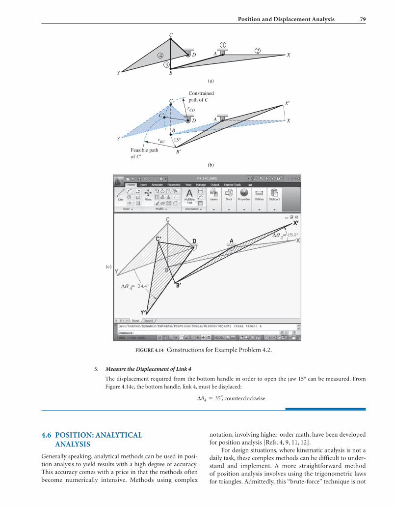
Position and Displacement Analysis 79
D
Y
(a)
C
A
B
X4
3
12
D
Y
(b)
C
A
Constrainedpath of C
Feasible pathof C′
B
B′
15°
C′X
X′
rBC
rCD
(c)
FIGURE 4.14 Constructions for Example Problem 4.2.
5. Measure the Displacement of Link 4
The displacement required from the bottom handle in order to open the jaw 15° can be measured. From
Figure 4.14c, the bottom handle, link 4, must be displaced:
¢u4 = 35°, counterclockwise
4.6 POSITION: ANALYTICAL ANALYSIS
Generally speaking, analytical methods can be used in posi-tion analysis to yield results with a high degree of accuracy.This accuracy comes with a price in that the methods oftenbecome numerically intensive. Methods using complex
notation, involving higher-order math, have been developedfor position analysis [Refs. 4, 9, 11, 12].
For design situations, where kinematic analysis is not adaily task, these complex methods can be difficult to under-stand and implement. A more straightforward methodof position analysis involves using the trigonometric lawsfor triangles. Admittedly, this “brute-force” technique is not

80 CHAPTER FOUR
30°
40Dimensions are in millimeters
50
FIGURE 4.15 Toggle clamp for Example Problem 4.3.
EXAMPLE PROBLEM 4.3
Figure 4.15 shows a toggle clamp used to securely hold parts. Analytically determine the displacement of the clamp
surface as the handle rotates downward, 15°.
efficient for those involved in kinematic research. However,for the typical design engineer, the simplicity far outweighsall inefficiencies. Thus, this triangle method of positionanalysis will be used in this text.
In general, this method involves inserting reference lineswithin a mechanism and analyzing the triangles. Laws of gen-eral and right triangles are then used to determine the lengthsof the triangle sides and the magnitude of the interior angles.As details about the geometry of the triangles are determined,this information is assembled to analyze the entire mechanism.
A substantial benefit of analytical analysis is the abilityto alter dimensions and quickly recalculate a solution.During the design stages, many machine configurations anddimensions are evaluated. Graphical analysis must be com-pletely repeated for each evaluation. Analytical methods,specifically when implemented with spreadsheets or othercomputer-based tools, can update solutions quickly.
The analytical method of position analysis can best beseen through the following examples.
SOLUTION: 1. Draw a Kinematic Diagram
The kinematic diagram is given in Figure 4.16a. The end of the handle was labeled as point of interest .X
A
B
(a)
(b)
X
C
A
B
40
30°
50
C
3
4
1
2
(c)
A
B′40 15°50
C
FIGURE 4.16 Mechanism for Example Problem 4.3.

Position and Displacement Analysis 81
γ
θ2 θ3
L2L3
L4
FIGURE 4.17 In-line slider-crank mechanism.
2. Analyze the Geometry in the Original Configuration
For this slider-crank mechanism, a triangle is naturally formed between pin joints , , and . This triangle is
shown in Figure 4.16b.
Prior to observing the mechanism in a displaced configuration, all properties of the original configuration
must be determined. The internal angle at joint , , can be determined from the law of sines,
equation (3.6):
The interior angle at joint , , can be found because the sum of all interior angles in any triangle
must total 180°:
The length side AC represents the original position of the slider and can be determined from the law of
cosines, equation (3.7):
3. Analyze the Geometry in the Displaced Configuration
The displaced configuration is shown in Figure 4.16c when the handle is rotated downward 15°. Note that this
displacement yields an interior angle at joint , , of 15°. The law of sines can be used to find the interior
angle at joint , :
Again, the interior angle at joint , , can be found because the sum of all interior angles in any
triangle must total 180°:
The length side represents the displaced position of the slider. As before, it can be determined from the
law of cosines:
4. Calculate the Desired Displacement
The displacement of point during this motion can be found as the difference of the triangle sides and AC:
¢RC = AC œ - AC = 86.14 - 74.52 = 11.62 mm ;ACœC
= 86.14 mm
= 3(50 mm)2 + (40 mm)2 - 2(50 mm)(40 mm)cos(146.12 �) = 86.14 mm
AC œ = 3ABœ2 + B œCœ2 - 2(ABœ) (BœCœ) cos∠ABœC œ
AC œ
∠AB œC œ = 180° - (15° + 18.88°) = 146.12°
∠AB œC œB œ
∠BœC œA = sin-1 c a ABœ
B œC œ b sin∠C œABœ d = sin-1 c a 50 mm
40 mmb sin 15°d = 18.88°
∠B œC œAC œ∠C œABœA
= 74.52 mm
= 3(50 mm)2 + (40 mm)2 - 2(50 mm)(40 mm){cos 111.32°}
AC = 3AB2 + BC2 - 2(AB ) (BC )cos∠ABC
∠ABC = 180° - (30° + 38.68°) = 111.32°
∠ABCB
∠BCA = sin-1 c a AB
BCb sin∠B AC d = sin-1 c a 50 mm
40 mmb sin 30°d = 38.68°
sin∠BAC
(BC)=
sin∠BCA
(AB)
∠BCAC
CBA
4.6.1 Closed-Form Position AnalysisEquations for an In-Line Slider-Crank
The clamp mechanism in Example Problem 4.3 is a slider-crank linkage. Specifically, it is termed an in-line slider-crankmechanism because the constrained path of the pin joint onthe slider extends through the center of the crank rotation.Figure 4.17 illustrates the basic configuration of an in-lineslider-crank linkage.

82 CHAPTER FOUR
EXAMPLE PROBLEM 4.4
Figure 4.18 shows a concept for a hand pump used for increasing oil pressure in a hydraulic line. Analytically
determine the displacement of the piston as the handle rotates 15° counterclockwise.
5''
4''
1''
10°
FIGURE 4.18 Toggle clamp for Example Problem 4.4.
(4.4)
(4.5)
These equations can be used to determine the position ofthe links in any configuration of an in-line slider-crankmechanism.
L4 = 3L22 + L3
2 - 2(L2) (L3)cos g
g = 180° - (u2 + u3)Because this is a common mechanism, the results fromthe previous problem can be generalized [Ref. 12]. A typicalanalysis involves locating the position of the links, giventheir lengths and and the crank angle .Specifically, the position of the slider and the interiorjoint angles and must be determined.
The equations used in Example Problem 4.3 aresummarized in terms of , , and :
(4.3)u3 = sin-1 c L2
L3 sin u2 du2L3L2
u)(u3
(L4)(u2)L3)(L2
SOLUTION: 1. Draw a Kinematic Diagram
The kinematic diagram is given in Figure 4.19a. The end of the handle was labeled as point of interest .X
E
DF
A AF
B B′
E′C′
D′
LC
A
(a) (b) (c)
2
B
C C4
3
10°10°
80°Offset 65°
25°LC′
FIGURE 4.19 Mechanism diagrams for Example Problem 4.4.
2. Analyze the Geometry in the Original Configuration
In contrast to the previous problem, this mechanism is an offset slider-crank mechanism. For this type of mech-
anism, it is convenient to focus on two right triangles. These triangles are shown in Figure 4.19b. Notice that the
10° angle and its 80° complement are shown.

Position and Displacement Analysis 83
Prior to observing the mechanism in a displaced configuration, all properties of the original configuration
must be determined. Focusing on the lower right triangle, the sides AD and BD can be determined from the fol-
lowing trigonometric functions:
By focusing on the top triangle, the length of side CE can be found as the sum of the offset distance and the
length of side AD from the lower triangle:
Use the Pythagorean theorem, equation (3.4), to determine side BE:
The original position of the piston, point , can be determined by summing BD and BE:
Although not required in this problem, the angle that defines the orientation of link 3 is often desired. The
angle can be determined with the inverse cosine function:
3. Analyze the Geometry in the Displaced Configuration
The displaced configuration is shown in Figure 4.19c with the handle rotated downward 15°. Note that this dis-
placement yields an angle at joint of 25°, and its complement, 65°, is also shown. Focusing on the lower right
triangle, the sides and can be determined from the following trigonometric functions:
Focusing on the top triangle, the length of side can be found as the sum of the offset distance (AF) and
the length of side from the lower triangle:
Side can then be determined:
The displaced position of the piston can be determined by summing and :
4. Calculate the Resulting Displacement
The displacement of the piston, point , during this motion can be found by subtracting the length
from :
¢RC = 8.46 - 7.05 = 1.41 in. T
LC
LCœC
L œC = B œD œ + B œE œ = 4.53 + 2.52 = 7.05 in.
B œE œB œD œ
B œE œ = 3(B œC œ )2 - (CœEœ )2 = 3(4 in.)2 - (3.11 in.)2 = 2.52 in.
B œE œ
= 1.0 + 2.11 = 3.11 in.
C œE œ = AF + AD œ
AD œC œE œ
B œD œ = (ABœ) sin∠B œAD œ = (5 in.) {sin 65°} = 4.53 in.
AD œ = (AB œ)cos∠B œAD œ = (5 in.) {cos 65° } = 2.11 in.
B œD œAD œA
∠BCE = cos-1aCE
BCb = cos-1 a 1.87 in.
4 in.b = 62.13°
∠BCE
LC = BD + BE = 4.92 + 3.54 = 8.46 in.
C
= 3(4)2 - (1.87)2 = 3.54 in.
BE = 3BC2 - CE 2
CE = offset + AD = 1.0 + 0.87 = 1.87 in.
BD = (AB) sin∠BAD = (5 in.) {sin 80°} = 4.92 in.
sin∠BAD =BD
AB
AD = (AB)cos∠BAD = (5 in.) {cos 80°} = 0.87 in.
cos∠BAD =AD
AB

84 CHAPTER FOUR
4.6.2 Closed-Form Position AnalysisEquations for an Offset Slider-Crank
The mechanism in Example Problem 4.4 is an offset slider-crank mechanism because the constrained path of the pinjoint on the slider does not extend through the center of thecrank rotation. Figure 4.20 illustrates the basic configurationof an offset slider-crank linkage.
A typical analysis involves locating the position of the links,given the lengths , , and and a crank angle .Specifically, the position of the slider and the interiorjoint angles and must be determined.
The generalized equations are given as
(4.6)
(4.7)
(4.8)
These equations can be used to determine the positionof the links in any mechanism configuration. Recall, how-ever, that these equations are only applicable to an offsetslider-crank mechanism. The equations also apply when theoffset distance is in the opposite direction as shown inFigure 4.20. For these cases, L1 in equation (4.6) should besubstituted as a negative value.
g = 180� - (u2 + u3)
L4 = L2 cos u2 + L3 cos u3
u3 = sin-1 c L1 + L2 sin u2
L3d
u)(u3
(L4)(u2)L3)L2(L1
EXAMPLE PROBLEM 4.5
Figure 4.21 shows a toggle clamp used for securing a workpiece during a machining operation. Analytically determine
the angle that the handle must be displaced in order to lift the clamp arm 30° clockwise.
γ2θ
θ3
L2
L1
L3
L4
FIGURE 4.20 Offset slider-crank mechanism.
Clamp arm
25 mm
15 mm
12 mm
90°
20 mmHandle
FIGURE 4.21 Clamp for Example Problem 4.5.
SOLUTION: 1. Draw a Kinematic Diagram
The kinematic diagram for the clamp is given in Figure 4.22a. The end of the handle was labeled as point of
interest . The clamp nose was identified as point of interest .
2. Analyze the Geometry in the Original Configuration
This mechanism is the common four-bar linkage. In order to more closely analyze the geometry, Figure 4.22b
focuses on the kinematic chain ABCD. A diagonal is created by connecting and , forming two triangles.
Prior to observing the mechanism in a displaced configuration, all properties of the original configuration
must be determined. Notice that the lower triangle, ABD, is a right triangle. The length of BD can be found using
the Pythagorean theorem introduced in equation (3.4).
The internal angles, and , can be determined from the following basic trigonometric
functions:
∠BDA = cos-1 a 25 mm
27.73 mmb = 25.6°
∠ABD = sin-1 a 25 mm
27.73 mmb = 64.4°
∠BDA∠ABD
BD = 3(AB)2 + (AD) 2 = 3(12)2 + (25)2 = 27.73 mm
DB
YX
Because this is also a common mechanism, the resultsfrom the previous problem can be generalized [Ref. 12].

Position and Displacement Analysis 85
B
B
C
C
D
D
A
A
Y
X
25
20
1215
3
4
4
A
B
(a) Kinematic diagram
(b) Original configuration
2
B′
B′
C′
DA25
20
12
60°
90°
90°
90°96.1°
6.1°
15
(d) Interior angel at B
A
13.3°
133.3°
120°
60°
(c) Displaced configuration
FIGURE 4.22 Mechanism for Example Problem 4.5.
Focusing on the top triangle, the internal angle can be found from the law of cosines, introduced in
equation (3.7):
The internal angle can be determined from the law of sines:
= sin-1 c a 15 mm
27.73 mmb sin 103.9°d = 31.7°
∠CBD = sin-1 c a CD
BDb sin ∠BCD d
∠CBD
= cos-1 a (20 mm)2 + (15 mm)2 - (27.73 mm)2
2(20 mm) (15 mm)b = 103.9°
∠BCD = cos-1 aBC2 + CD2 - BD2
2(BC) (CD)b
∠BCD

86 CHAPTER FOUR
The interior angle at can be found because the sum of all interior angles in any triangle must total
180°. Thus
The total mechanism angles at joint (between links 2 and 3) and at joint (between links 1 and 4) can be
determined.
At joint B:
At joint D:
3. Analyze the Geometry in the Displaced Configuration
The displaced configuration is shown in Figure 4.22c with the clamp nose, link 2, rotated clockwise 30°. Notice
that this leaves the interior angle at joint , , as 60°. Also, the lower triangle is no longer a right triangle.
The length of diagonal can be found by using the lower triangle, , and the law of cosines:
The internal angle can also be determined from the law of cosines:
The total of the interior angles of any triangle must be 180°. Therefore, angle can be readily
determined:
Focusing on the top triangle, the internal angle can be found from the law of cosines:
The internal angle can be determined from the law of sines:
The final interior angle, , of the upper triangle can be found by the following:
The total mechanism angles at joint (between links 2 and 3) and at joint (between links 1 and 4) can be
determined by the following:
At joint B’:
At joint D:
∠C œDA = ∠B œDC œ + ∠B œDA = 63.1° + 28.7°= 91.8°
∠AB œC œ = ∠AB œD + ∠C œB œD = 91.3° + 42.0° = 133.3°
DB
∠B œDC œ = 180° - (∠C œB œD + ∠B œC œD) = 180° - (42.0° + 74.9°) = 63.1°
∠B œDC œ
= sin-1 c a 15 mm
21.66 mmb sin 74.9� d = 42.0�
∠C œB œD = sin-1 c a C œD
B œDb sin∠B œC œD d
∠C œB œD
= cos-1 c (20 mm)2 + (15 mm)2 - (21.66 mm)2
2(20 mm)(15 mm)d = 74.9�
∠B œC œD = cos-1 c (B œC œ)2 + (C œD)2 - (B œD)2
2(B œC œ)(C œD)d
∠B œC œD
= 180° - (60° + 91.3°) = 28.7°
∠B œDA = 180° - (∠DAB œ + ∠AB œD)
∠B œDA
= cos-1 c (12)2 + (21.66)2 - (25)2
2(12) (21.66)d = 91.3°
∠ABœD = cos-1 (AB)2 + (BœD)2 - (AD)2
2(AB œ) (B œD)
∠ABœD
B œD = 3(12 mm)2 + (25 mm)2 - 2(12 mm)(25 mm) cos 60° = 21.66 mm
¢ABDB œD
∠DABœA
∠CDA = ∠BDC + ∠BDA = 44.4° + 25.6° = 70.0°
∠ABC = ∠ABD + ∠CBD = 64.4° + 31.7° = 96.1°
DB
∠BDC = 180° - 1103.9° + 31.7°2 = 44.4°
∠BDC

Position and Displacement Analysis 87
A
B
C
D
L1
L3
L2L43
2
θθ θ4
γ
FIGURE 4.23 The four-bar mechanism.
4.6.3 Closed-Form Position Equations for a Four-Bar Linkage
The four-bar mechanism is another very common linkage.Figure 4.23 illustrates a general four-bar linkage.
disassembled. The mechanism shown in Figure 4.23operates in the first circuit (Figure 4.24a).
Circuit 1
(a)
Circuit 2
(b)
FIGURE 4.24 Circuits of a four-bar mechanism.
The specific equations used in Example Problem 4.5 canbe generalized [Ref. 12]. A typical analysis involves determi-ning the interior joint angles , , and for known links
, , , and at a certain crank angle . Specifically,the interior joint angles , , and must be determined.
(4.9)
(4.10)
(4.11)
(4.12)
These equations can be used to determine the positionof the links in any mechanism configuration. The equationsare applicable to any four-bar mechanism assembled asshown in Figure 4.23.
4.6.4 Circuits of a Four-Bar Linkage
For four-bar mechanisms classified as crank-rockers (asdescribed in Section 1.10), there are two regions of possiblemotion corresponding with the two geometric inversions.These regions are termed assembly circuits. A mechanism isunable to move between assembly circuits without being
u4 = 2 tan -1 c L2 sin u2 - L3 sin g
L2 cos u2 + L4 - L1 - L3 cos gd
u3 = 2 tan -1 c -L2 sin u2 + L4 sin g
L1 + L3 - L2 cos u2 - L4 cos gd
g = cos-1 c (L3)2 + (L4)2 - (BD)2
2(L3) (L4)d
BD = 3L12 + L2
2 - 2(L1) (L2)cos(u2)
g)u4(u3
(u2)L4)L3L2(L1
g)u4(u3
By physically disconnecting joint , the links can bereoriented and reassembled into the configuration shown inFigure 4.24b. As this mechanism is operated, it exhibitsmotion in the second circuit. Although the motion of themechanism appears to be different, depending on the circuitof operation, the relative motion between the links does notchange. However, the circuit in which the mechanism isassembled must be specified to understand the absolutemotion and operation of the mechanism.
For four-bar mechanisms operating in the secondcircuit, equation (4.11) must be slightly altered as follows:
(4.13)
(4.14)
4.7 LIMITING POSITIONS: GRAPHICALANALYSIS
The configuration of a mechanism that places one of thefollower links in an extreme location is called a limitingposition. Many machines have linkages that continuallyoscillate between two limiting positions. Figure 4.25 illustratesthe limiting positions of an offset slider-crank mechanism.
u4 = 2 tan -1 c L2 sin u2 + L3 sin g
L2 cos u2 + L4 - L1 - L3 cos gd
u3 = 2 tan -1 c -L2 sin u2 - L4 sin g
L1 + L3 - L2 cos u2 - L4 cos gd
C
4. Calculate the Resulting Displacement
The angular displacement of the handle, link 3, can be determined by focusing on joint , as shown in
Figure 4.22d. For the original configuration, the angle of link 3 above the horizontal is expressed as
For the displaced configuration, the angle of link 3 above the horizontal is expressed as
Finally, the angular displacement of link 3 is determined by
¢u3 = 13.3° - 6.1° = 7.2°, counterclockwise
∠AB œC œ - 120° = 133.3° - 120.0° = 13.3°
∠ABC - 90° = 96.1° - 90.0° = 6.1°
B

88 CHAPTER FOUR
The displacement of the follower link from one limitingposition to the other defines the stroke of the follower. Fortranslating links, as shown in Figure 4.25a, the stroke is a linearmeasurement. For links that exhibit pure rotation, the stroke isan angular quantity, and is also called throw, as shown inFigure 4.25b. The configuration of links that place a follower ina limiting position is associated with the crank and couplerbecoming collinear. Figure 4.25 illustrates the limiting configu-rations for a slider-crank and a four-bar linkage. An imbalanceangle is defined as the angle between the coupler configura-tion at the two limiting positions. The imbalance angle influ-ences the timing of the inward and outward stroke and will beextensively utilized in Chapter 5. The position of a driver, oractuated link, that places a follower link in an extreme, or lim-iting, position is often desired. In addition, the motion of alinkage is commonly referenced from the actuator positionthat places the follower in a limiting position.
The logic used on solving such a problem is similar tothe position analysis just discussed. The following examplesillustrate this analysis.
b
EXAMPLE PROBLEM 4.6
The mechanism shown in Figure 4.26 is the driving linkage for a reciprocating saber saw. Determine the configura-
tions of the mechanism that places the saw blade in its limiting positions.
1.0"
1.75"
.5"
FIGURE 4.26 Saber saw mechanism for Example Problem 4.6.
SOLUTION: 1. Draw a Kinematic Diagram
The kinematic diagram for the reciprocating saw mechanism is given in Figure 4.27a. Notice that this is a slider-
crank mechanism as defined in Chapter 1. The slider-crank has one degree of freedom.
2. Construct the Extended Limiting Position
The saw blade, link 4, reaches its extreme downward position as links 2 and 3 move into a collinear alignment.
This configuration provides the maximum distance between points and . To determine this maximum
distance, the lengths of links 2 and 3 must be combined. Adding these lengths,
Once the combined length of lines 2 and 3 is determined, an arc should be constructed of this length,
centered at point . As shown in Figure 4.29b, the intersection of this arc and the possible path of point A
L2 + L3 = 0.5 in. + 1.75 in. = 2.25 in.
CA
(a) Slider-crank
Stroke, |ΔRC|max
B'
A B''
C' C C''
B
β
(b) Four-bar
B'
Aβ
D Throw, (θ4)max
B''
C' C
C''B
FIGURE 4.25 Limiting positions.

Position and Displacement Analysis 89
A
B
C
(b)(a)
2
4
31
A
B
C
L3– L2
C′
C″
2
4
31
L2+
L1
L3
L1L2
L3
(c)
FIGURE 4.27 Extreme positions for Example Problem 4.6.
This retracted limiting position can be determined using a technique similar to determining the extended
position. Recall that the distance between and in Figure 4.27b represents the combined length of links 2 and
3. Similarly, the distance between points and represents the difference between links 3 and 2.
Using the distance, the position of point at its extreme upward position, denoted as , can be
determined (Figure 4.27b). Finally, links 2 and 3 can be drawn and the position of point is located.
4. Measure the Stroke of the Follower Link
As shown in Figure 4.27c, the stroke of the saw blade can be measured as the extreme displacement of point .
Scaling this from the kinematic diagram yields the following result:
ƒ ¢RC ƒ max = 1.27 in.
C
BœœC œœCL3 - L2
C œœA
CœA
determines the limiting extended position of C, denoted C. Links 2 and 3 can be drawn, and point can be
determined. This is shown in Figure 4.29c.
3. Construct the Retracted Limiting Position
Next, the configuration that places the saw blade, link 4, in its extreme upper position must be determined. In
this configuration, links 2 and 3 are again collinear but overlapped. This provides the minimum distance
between points and . Thus, this minimum distance is the difference between the lengths of links 3 and 2.
Subtracting the link lengths gives
L3 - L2 = 1.75 in. - 0.5 in. = 1.25 in.
CA
Bœ

90 CHAPTER FOUR
A
D
B
L2 + L3
L2
L4
L3
L3 – L2
C
(b)(a)
2
4
3
1A
D
B
C
C
C
(c)
FIGURE 4.29 Extreme positions for Example Problem 4.7.
Motor
Water inlet
Nozzle
2.0"
2.0"
2.0"
1.0" .75"
FIGURE 4.28 Water nozzle linkage for Example Problem 4.7.
SOLUTION: 1. Draw the Kinematic Diagram
The kinematic diagram for the water nozzle linkage is given in Figure 4.29. Notice that this is a four-bar
mechanism with one degree of freedom.
2. Construct the Extended Limiting Position
The analysis in this example is very similar to Example Problem 4.6. The nozzle, link 4, reaches its extreme
downward position as links 2 and 3 become collinear. This configuration provides the maximum distance
between points and . To determine this maximum distance, the lengths of links 2 and 3 must be combined.
Adding these lengths gives
L2 + L3 = 0.75 in. + 2.00 in. = 2.75 in.
CA
EXAMPLE PROBLEM 4.7
Figure 4.28 illustrates a linkage that operates a water nozzle at an automatic car wash. Determine the limiting
positions of the mechanism that places the nozzle in its extreme positions.

Position and Displacement Analysis 91
Once the combined length of lines 2 and 3 is determined, an arc should be constructed of this length,
centered at point A. As shown in Figure. 4.28b, the intersection of this arc and the possible path of point C
determines the extreme downward position of C, denoted . Links 2 and 3 can be drawn, and point can be
determined. This is shown in Figure 4.29c.
3. Construct the Retracted Limiting Position
Next, the configuration that places the nozzle, link 4, in its extreme upper position must be determined.
Similar to the slider-crank discussed in Example Problem 4.6, the retracted configuration occurs when
links 2 and 3 are collinear but overlapped. This produces the minimum distance between points A and C.
Thus, this minimum distance is the difference between the lengths of links 3 and 2. Subtracting the link
lengths gives
This minimum distance can be constructed similar to the technique for the maximum distance. Recall that
the distance between A and in Figure 4.29c represents the combined length of links 2 and 3. Similarly, the
distance between points A and represents the difference between links 3 and 2.
Using the distance, the position of point at its extreme upward position, denoted as , can be
determined. This is shown in Figure 4.29b. Finally, links 2 and 3 can be drawn and the position of point is
located.
4. Measure the Stroke of the Follower Link
As shown in Figure 4.29c, the stroke of the nozzle can be measured as the extreme angular displacement of link
4. Measuring this from the graphical layout yields the following:
ƒ ¢u4 ƒ max = 47.0°
BœœC œœCL3 - L2
C œœC œ
L3 - L2 = 2.00 in. - .75 in. = 1.25 in.
BœC œ
4.8 LIMITING POSITIONS: ANALYTICALANALYSIS
Analytical determination of the limiting positions for amechanism is a combination of two concepts presentedearlier in this chapter:
I. The logic of configuring the mechanism into a limitingconfiguration. This was incorporated in the graphicalmethod for determining the limiting positions, aspresented in Section 4.7.
II. The method of breaking a mechanism into convenienttriangles and using the laws of trigonometry to deter-mine all mechanism angles and lengths, as presented inSection 4.6.
Combining these two concepts to determine theposition of all links in a mechanism at a limiting position isillustrated through Example Problem 4.8.
EXAMPLE PROBLEM 4.8
Figure 4.30 shows a conveyor transfer mechanism. Its function is to feed packages to a shipping station at specific in-
tervals. Analytically determine the extreme positions of the lifting conveyor segment.
SOLUTION: 1. Draw the Kinematic Diagram
The kinematic diagram for the mechanism is given in Figure 4.31a. The end of the conveyor segment is labeled
as point of interest .
2. Analyze the Geometry at the Extended Limiting Position
This mechanism is another four-bar linkage. As seen in Example Problem 4.7, the follower of a four-bar is in the
extended limiting position when links 2 and 3 become collinear. Figure 4.31b illustrates this mechanism with the
follower in its upper position. Notice that the links form a general triangle, . Also note that the length of
is 20 in. .(16 + 4)AC œ¢AC œD
X

92 CHAPTER FOUR
X
A
2
B
CD4
3
1
A
18
16
20
(b)(a)
B'
C'
8
4
D
A
18
(c)
B'
C''8
4
D
16
12
FIGURE 4.31 Mechanism for Example Problem 4.8.
18'' 16''
4 ''
8'' 10''
FIGURE 4.30 Conveyor feed for Example Problem 4.8.
This upper-limiting position is fully defined by determination of the internal angles. The internal angle at
joint , , can be found using the law of cosines:
The law of sines can be used to find either of the remaining internal angles. However, the law of sines may
present some confusion with angles between 90° and 180° because
When the inverse sine function is used on a calculator, an angle is between 0° and 90°. However, the desired
result may be an angle between 90° and 180°. To minimize this confusion, it is recommended to draw the trian-
gles to an approximate scale and verify numerical results. Also, it is best to use the law of sines with angles that
are obviously in the range of 0° to 90°.
Using that approach, the internal angle at joint , , is determined using the law of sines because it
is obviously smaller than 90°.
The internal angle at joint , , can be determined:
= 180° - (23.6° + 64.1°) = 92.3°
∠ADC œ = 180° - (∠C œAD + ∠ADC œ)
∠ADCœD
= sin-1 c a18 in.
8 in.b sin 23.6° d = 64.1°
∠ACœD = sin-1 c aAD
DCœb sin∠CœAD d
∠AC œDC œ
sin u = sin(180° - u)
= cos-1 c (18 in.)2 + (20 in.)2 - (8 in.)2
2(18 in.) (20 in.)d = 23.6°
∠C œAD = cos-1 cAD 2 + AC œ - C œD 2
2(AD) (AC œ)d
∠CœADA

Position and Displacement Analysis 93
3. Analyze the Geometry at the Retracted Limiting Position
Figure 4.31c illustrates this mechanism with the follower in its lower position. Again, the links form a general tri-
angle, . Notice that the length of AC'' is 12 in. (16 – 4).
To fully define this configuration, the internal angles are determined through a procedure identical to the
one just described.
For the internal angle at joint , :
The internal angle at is in the range of 0° to 90°. Therefore, for the internal angle at joint , :
Finally, the internal angle at joint , , can be determined by the following:
4. Measure the Stroke of the Follower Link
To summarize, the conveyor segment (internal angle at joint cycles between 92.3° and 32.1°, as
measured upward from the vertical:
and the stroke is
ƒ ¢u4 ƒ max = 92.3° - 32.1° = 60.2°
32.1° 6 u4 6 92.3°
D, ∠ADC)
= 180° - (20.7° + 32.1°) = 127.2°
∠AC œœD = 180° - (∠C œœAD + ∠ADC œœ)
D∠AC œœC œœ
= sin-1 ca12 in.
8 in.b sin 20.7°d = 32.1°
∠ADC œœ = sin-1 c aAC œ
DC œb sin∠C œœADd∠ADCœœDD
= cos-1 c (18 in.)2 + (12 in.)2 - (8 in.)2
2(18 in.) (12 in.)d = 20.7°
∠C œœAD = cos-1 cAD 2 + AC œ2 - C œœD 2
2(AD ) (ACœœ)d
∠C œœADA
¢AC œD
4.9 TRANSMISSION ANGLE
The mechanical advantage of a mechanism is the ratio of theoutput force (or torque) divided by the input force (ortorque). In a linkage, the transmission angle quantifies theforce transmission through a linkage and directly affects themechanical efficiency. Clearly, the definitions of trans-mission angle depend on the choice of driving link. Thetransmission angle for slider-crank and four-bar mecha-nisms driven by the crank is shown in Figure 4.32. In theselinkages, the mechanical advantage is proportional to thesine of the angle . As the linkage moves, the transmissionangle, along with all other joint angles, and the mechanicaladvantage constantly change. Often, the extreme trans-mission angle values are desired.
In the slider-crank, the transmission angle is measuredbetween the coupler and a line normal to the slidingdirection. The values for the minimum and maximumtransmission angles can be determined by geometricallyconstructing the configurations as shown in Figure 4.32a.Alternatively, the minimum and maximum transmissionangles for a slider-crank can be calculated from
g
g
(4.15)
(4.16)
In the four-bar, the transmission angle is measuredbetween the output link and the coupler. As with the slider-crank, the values for the minimum and maximum trans-mission angles can be determined by geometricallyconstructing the configurations as shown in Figure 4.32b.Alternatively, the minimum and maximum transmissionangles can be calculated from
(4.17)
(4.18)
The transmission angle is one measure of the qualityof force transmission in the mechanism. Ordinarily, the
g max = cos -1 c L32 + L4
2 - 1L1 + L2222L3 L4
d
g min = cos -1 c L32 + L4
2 - 1L1 - L2222 L3 L4
d
g max = cos -1 cL1 - L2
L3d
g min = cos -1 cL1 + L2
L3d
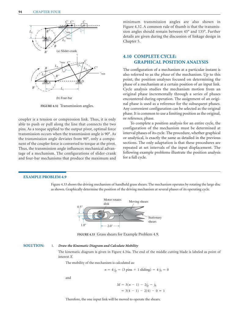
94 CHAPTER FOUR
coupler is a tension or compression link. Thus, it is onlyable to push or pull along the line that connects the twopins. As a torque applied to the output pivot, optimal forcetransmission occurs when the transmission angle is 90°. Asthe transmission angle deviates from 90°, only a compo-nent of the coupler force is converted to torque at the pivot.Thus, the transmission angle influences mechanical advan-tage of a mechanism. The configurations of slider-crankand four-bar mechanisms that produce the maximum and
minimum transmission angles are also shown inFigure 4.32. A common rule of thumb is that the transmis-sion angles should remain between 45° and 135°. Furtherdetails are given during the discussion of linkage design inChapter 5.
4.10 COMPLETE CYCLE:GRAPHICAL POSITION ANALYSIS
The configuration of a mechanism at a particular instant isalso referred to as the phase of the mechanism. Up to thispoint, the position analyses focused on determining thephase of a mechanism at a certain position of an input link.Cycle analysis studies the mechanism motion from anoriginal phase incrementally through a series of phasesencountered during operation. The assignment of an origi-nal phase is used as a reference for the subsequent phases.Any convenient configuration can be selected as the originalphase. It is common to use a limiting position as the original,or reference, phase.
To complete a position analysis for an entire cycle, theconfiguration of the mechanism must be determined atinterval phases of its cycle. The procedure, whether graphicalor analytical, is exactly the same as detailed in the previoussections. The only adaptation is that these procedures arerepeated at set intervals of the input displacement. Thefollowing example problems illustrate the position analysisfor a full cycle.
(a) Slider-crank
γmax
γ
γmin
γmax
γmin γ
B'
A
L1
L2 L3
L3 L4
L2
L1
B''
C' C'' C
B
(b) Four-bar
B'
A D
B''
C' C
C''B
FIGURE 4.32 Transmission angles.
EXAMPLE PROBLEM 4.9
Figure 4.33 shows the driving mechanism of handheld grass shears. The mechanism operates by rotating the large disc
as shown. Graphically determine the position of the driving mechanism at several phases of its operating cycle.
Motor rotatesdisk
Moving shears
Stationaryshears
2.0"
0.5"
1.0"
FIGURE 4.33 Grass shears for Example Problem 4.9.
SOLUTION: 1. Draw the Kinematic Diagram and Calculate Mobility
The kinematic diagram is given in Figure 4.34a. The end of the middle cutting blade is labeled as point of
interest .
The mobility of the mechanism is calculated as:
and
Therefore, the one input link will be moved to operate the shears.
= 3(4 - 1) - 2(4) - 0 = 1
M = 3(n - 1) - 2jp - jh
n = 4 jp = (3 pins + 1 sliding) = 4 jh = 0
X

Position and Displacement Analysis 95
(a)
(b)
2. Designate the Reference Phase
To assign a reference phase, only the position of the input link must be specified. Arbitrarily select the configu-
ration when the drive disk, link 2, is in a vertical position, with joint directly below joint .
3. Construct Interval Phases
Drawing the mechanism in several phases of its cycle is identical to the previous position analysis, but repetitive.
While drawing the different phases using graphical methods, the kinematic diagram can become cluttered very
AB
FIGURE 4.34 Mechanism phases for Example Problem 4.9.

96 CHAPTER FOUR
quickly. It is highly recommended that different colors or fonts be used to represent each phase of the cycle. When
using CAD, it is also beneficial to place each phase on a different layer, which can be rapidly displayed or hidden.
For this problem, the driving link, link 2, is positioned at 45° intervals throughout its cycle. Therefore, eight
phases of the mechanism are constructed. The phases are designated as phase 1 through 8. The eight positions of
points and are shown in Figure 4.34b. Notice that the points are identified by using a subscript from 1 to 8,
matching the corresponding phase. In practice, even smaller increments are used depending on the details of the
mechanism motion that is required.
4. Construct the Limiting Positions
The phases associated with the limiting positions should also be determined. The shear blade reaches its
upwardmost position when link 4 rotates to the greatest angle possible. This occurs when link 4 is tangent to
the circle that represents the possible positions of point . The point of tangency is denoted as , and the
corresponding position of the blade is denoted as . This is shown in Figure 4.34c.
Similarly, the lowest position of the blade occurs when link 4 dips to its lowest angle. Again, this occurs
when link 4 is tangent to the circle that represents the possible paths of . The points related to this lowest
configuration are denoted in Figure 4.34c as and .
The maximum displacement of link 4 can be measured from the kinematic construction:
ƒ ¢u4 ƒ max = 29.0°
X œœBœœB
X œBœB
XB
(c)
4.11 COMPLETE CYCLE:ANALYTICAL POSITION ANALYSIS
To generate the configuration of a mechanism throughout acycle, analytical analysis can be repeated to obtain variousphases. This can be an extremely repetitious process and
the use of computer programs as discussed in Chapter 8 iscommon.
Equations, generated from triangles defined in part bythe mechanism links, can be summarized as in equations(4.1) through (4.12). These equations can be solved for vari-ous values of the driver position. Computer spreadsheets asdiscussed in Chapter 8 are ideal for such analyses.
FIGURE 4.34 Continued

Position and Displacement Analysis 97
EXAMPLE PROBLEM 4.10
Figure 4.35 shows a mechanism that is designed to push parts from one conveyor to another. During the transfer,
the parts must be rotated as shown. Analytically determine the position of the pusher rod at several phases of its
motion.
30
30
70
FIGURE 4.35 Conveyor feed for Example Problem 4.10.
L4
3θ
θ2
βA
B
L3 L2L1
C
FIGURE 4.36 Kinematic diagram for Example Problem 4.10.
SOLUTION: 1. Draw the Kinematic Diagram
The kinematic diagram for this mechanism is shown in Figure 4.36. Notice that it is an offset slider-crank
mechanism having one degree of freedom.
2. Designate the Original Phase
Arbitrarily, the original phase is selected to be when the crank is horizontal, placing joint directly left of
joint .
3. Construct the Interval Phases
Recall that equations (4.6), (4.7), and (4.8) describe the position of an offset slider-crank mechanism. These can
be used in a full-cycle analysis. The equations were used in conjunction with a spreadsheet, yielding the results
shown in Figure 4.37. If you are not familiar with using spreadsheets, refer to Chapter 8.
4. Identify the Limiting Positions
Focusing on the position of link 4, the slider oscillation can be approximated as
and the maximum displacement as
This is only an approximation because, at 15° increments, the limiting position cannot be precisely detected. When
exact information on the limiting position is required, the techniques discussed in Section 4.8 can be used.
Confusion may arise when observing the value of the angle at the crank angle, , of 360°. The value should be
identical to the initial value at the 0° crank angle. Note that the values differ by 360°. One is measuring the inner angle,
and the other is measuring the outer angle. This illustrates the need to verify the information obtained from the equa-
tions with the physical mechanism.
u2b
ƒ ¢R4 ƒ max = (L4)max - (L4)min � 93.25 - 26.51 = 66.74 mm
26.51 mm 6 L4 6 93.25 mm
A
B

98 CHAPTER FOUR
4.12 DISPLACEMENT DIAGRAMS
Once a full-cycle position analysis is completed, it is insight-ful to plot the displacement of one point correspondingto the displacement of another point. It is most common toplot the displacement of a point on the follower relative tothe displacement of a point on the driver.
Typically, the displacement of the driver is plotted onthe horizontal. In the case of a crank, the driver displace-ment consists of one revolution. The corresponding dis-placement of the follower is plotted along the vertical. Thedisplacement plotted on the vertical axis may be linear orangular depending on the motion obtained from the specificmechanism.
FIGURE 4.37 Positions of pusher rod for Example Problem 4.10.
EXAMPLE PROBLEM 4.11
Figure 4.38 shows the driving mechanism of a reciprocating compressor. Plot a displacement diagram of the piston
displacement relative to the crankshaft rotation.
SOLUTION: 1. Draw the Kinematic Diagram
After close examination, the compressor mechanism is identified as a slider-crank. Recall that this mechanism
has one degree of freedom and can be operated by rotating the crank. The kinematic diagram with the appropri-
ate dimensions is shown in Figure 4.39.

Position and Displacement Analysis 99
Intakegas
Exhaustgas
Cylinder
Cylinder head
Connecting rod
Piston
Crankshaft
Valve plate
.75''
2.0''
FIGURE 4.38 Compressor for Example Problem 4.11.
2A
B
2
Δ
θ
RC
C
3
1
4
2.0
.75
FIGURE 4.39 Kinematic diagram for Example Problem 4.11.
2. Designate the Reference Phase
As shown in Figure 4.39, the reference phase is arbitrarily selected as the crank is vertical, placing joint
directly above joint . The position of the piston (point will be measured from this reference
position.
3. Construct the Interval Phases
The actual displacements can be determined either analytically or graphically, using the methods
presented in the previous sections. For this slider-crank mechanism, the displacements were obtained
analytically using equations (4.3) through (4.5). Using a spreadsheet, the results were obtained as
shown in Figure 4.40. The crank displacement is in degrees and the piston displacement is in
inches.
4. Identify the Limiting Positions
Focusing on the position of the piston, the oscillation can be approximated as
As stated in the previous problem, this is only an approximation because, at 30° increments, the limiting
position will not be precisely detected. However, for the in-line slider-crank mechanism, inspecting the
geometry reveals that the limiting positions occur at crank angles of 0° and 180°. Therefore, the stroke is
exactly 1.50 in.
5. Plot the Displacement Diagram
The values calculated in the spreadsheet and tabulated in Figure 4.40 were plotted in Figure 4.41 to form a
displacement diagram.
ƒ ¢Rc ƒ max � 1.50 in.
(¢RC)(u2)
CAB

100 CHAPTER FOUR
FIGURE 4.41 Displacement diagram for Example Problem 4.11.
FIGURE 4.40 Position of displacement for Example Problem 4.11.
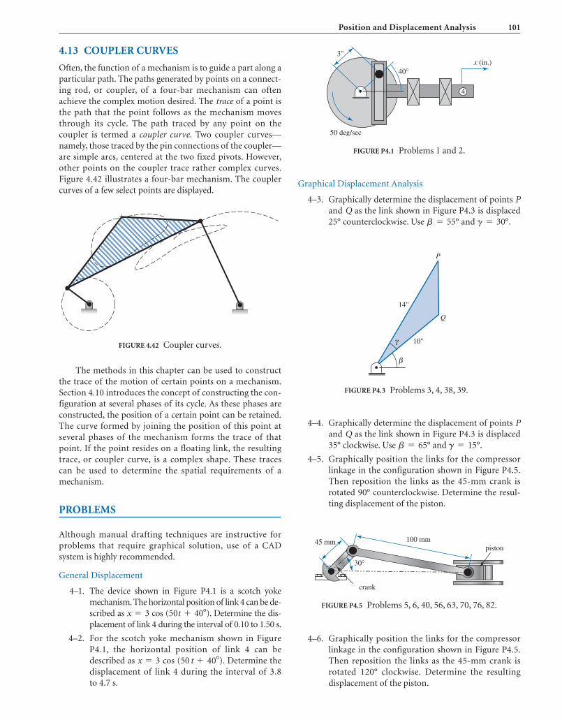
Position and Displacement Analysis 101
4.13 COUPLER CURVES
Often, the function of a mechanism is to guide a part along aparticular path. The paths generated by points on a connect-ing rod, or coupler, of a four-bar mechanism can oftenachieve the complex motion desired. The trace of a point isthe path that the point follows as the mechanism movesthrough its cycle. The path traced by any point on thecoupler is termed a coupler curve. Two coupler curves—namely, those traced by the pin connections of the coupler—are simple arcs, centered at the two fixed pivots. However,other points on the coupler trace rather complex curves.Figure 4.42 illustrates a four-bar mechanism. The couplercurves of a few select points are displayed.
The methods in this chapter can be used to constructthe trace of the motion of certain points on a mechanism.Section 4.10 introduces the concept of constructing the con-figuration at several phases of its cycle. As these phases areconstructed, the position of a certain point can be retained.The curve formed by joining the position of this point atseveral phases of the mechanism forms the trace of thatpoint. If the point resides on a floating link, the resultingtrace, or coupler curve, is a complex shape. These tracescan be used to determine the spatial requirements of amechanism.
PROBLEMS
Although manual drafting techniques are instructive forproblems that require graphical solution, use of a CADsystem is highly recommended.
General Displacement
4–1. The device shown in Figure P4.1 is a scotch yokemechanism. The horizontal position of link 4 can be de-scribed as cos ( ). Determine the dis-placement of link 4 during the interval of 0.10 to 1.50 s.
4–2. For the scotch yoke mechanism shown in FigureP4.1, the horizontal position of link 4 can bedescribed as cos ( ). Determine thedisplacement of link 4 during the interval of 3.8to 4.7 s.
50 t + 40°x = 3
50t + 40°x = 3
FIGURE 4.42 Coupler curves.
Graphical Displacement Analysis
4–3. Graphically determine the displacement of points and as the link shown in Figure P4.3 is displaced25° counterclockwise. Use and .g = 30°b = 55°
QP
4
x (in.)40°
3"
50 deg/sec
FIGURE P4.1 Problems 1 and 2.
P
Q
14"
10"
β
γ
FIGURE P4.3 Problems 3, 4, 38, 39.
4–4. Graphically determine the displacement of points and as the link shown in Figure P4.3 is displaced35° clockwise. Use and .
4–5. Graphically position the links for the compressorlinkage in the configuration shown in Figure P4.5.Then reposition the links as the 45-mm crank isrotated 90° counterclockwise. Determine the resul-ting displacement of the piston.
g = 15°b = 65°Q
P
45 mm
30°
crank
100 mmpiston
FIGURE P4.5 Problems 5, 6, 40, 56, 63, 70, 76, 82.
4–6. Graphically position the links for the compressorlinkage in the configuration shown in Figure P4.5.Then reposition the links as the 45-mm crank isrotated 120° clockwise. Determine the resultingdisplacement of the piston.

102 CHAPTER FOUR
4–7. Graphically position the links for the shearing mech-anism in the configuration shown in Figure P4.7.Then reposition the links as the 0.75-in. crank isrotated 100° clockwise. Determine the resulting dis-placement of the blade.
.75''
.5''
crank
50°
4''
blade
FIGURE P4.7 Problems 7, 8, 41, 57, 64, 71, 77, 83.
Handle
Stamp6''
6''
50°
4''
30°8''
FIGURE P4.9 Problems 9, 10, 42.
9''8''
15''
18''
10°
FIGURE P4.11 Problems 11, 12, 43.
4–11. Graphically position the links for the furnace doorin the configuration shown in Figure P4.11.Then reposition the links as the handle, which isoriginally set at 10°, is rotated counterclockwise to40°. Determine the resulting displacement of thedoor.
4–8. Graphically position the links for the shearingmechanism in the configuration shown in FigureP4.7. Then reposition the links as the blade is low-ered 0.2 in. Determine the resulting angular dis-placement of the crank.
4–9. Graphically position the links for the embossingmechanism in the configuration shown inFigure P4.9. Then reposition the links as the handleis rotated 15° clockwise. Determine the resultingdisplacement of the stamp and the linear dis-placement of the handle end.
4–10. Graphically position the links for the embossingmechanism in the configuration shown in FigureP4.9. Then reposition the links as the handle isrotated 10° counterclockwise. Determine theresulting displacement of the stamp and the lineardisplacement of the handle end.
4–12. Graphically position the links for the furnace doorin the configuration shown in Figure P4.11. Thenreposition the links as the door is raised 3 in.Determine the angular displacement of the handlerequired to raise the door 3 in.
4–13. A rock-crushing mechanism is given inFigure P4.13. Graphically position the links for theconfiguration shown. Then reposition the links asthe crank is rotated 30° clockwise. Determine theresulting angular displacement of the crushing ram.
360 mm
Crushing ram
180 mm
Crank
420 mm
60 mm75°
FIGURE P4.13 Problems 13, 14, 44, 58, 65, 72, 78, 84.
4–14. A rock-crushing mechanism is given in FigureP4.13. Graphically position the links for the con-figuration shown. Then reposition the links asthe crank is rotated 150° counterclockwise. Deter-mine the resulting angular displacement of thecrushing ram.
4–15. Graphically position the links for the rear-wipermechanism shown in Figure P4.15. Then repositionthe links as the 2-in. crank is rotated 50° clockwise.Determine the resulting angular displacement of thewiper arm and the linear displacement at the end ofthe wiper blade.

Position and Displacement Analysis 103
4–16. Graphically position the links for the rear-wipermechanism shown in Figure P4.15. Then repositionthe links as the 2-in. crank is rotated 110° clockwise.Determine the resulting angular displacement of thewiper arm and the linear displacement at the end ofthe wiper blade.
4–17. Graphically position the links for the vise gripsshown in Figure P4.17. Then reposition the links asthe top jaw is opened 40° from the orientationshown, while the lower jaw remains stationary.Determine the resulting angular displacement of thetop handle.
Wiper blade
8''
8''16''
13''
Wiper arm
70°50°
3.5''
14''
Crank
2''
FIGURE P4.15 Problems 15, 16, 45, 59, 66, 73, 79, 85.
4.2 cm
3.2 cm
7.0 cm
10.6 cm
20°
FIGURE P4.17 Problems 17, 18, 19, 46.
4–18. Graphically position the links for the vise gripsshown in Figure P4.17. Then reposition the links asthe top jaw is opened 20° from the orientationshown, while the lower jaw remains stationary.Determine the resulting angular displacement of thetop handle.
4–19. When the thumbscrew in the vise grips shown inFigure P4.17 is rotated, the effective pivot point ofthe 7.0-cm link is moved. During this motion, thespring prevents the jaws from moving. Graphicallyposition the links as the effective pivot point ismoved 2 cm to the right. Then reposition the linksas the top jaw is opened 40° from the new orienta-tion, while the lower jaw remains stationary.Determine the resulting angular displacement of thetop handle.
4–20. Graphically position the links for the small aircraftnosewheel actuation mechanism shown in FigureP4.20. Then reposition the links as the 12-in. crankis rotated 60° clockwise from the orientation shown.Determine the resulting angular displacement of thewheel assembly.
30''26''
30''
32''
5''12''
15°
FIGURE P4.20 Problems 20, 21, 47, 60, 67, 74, 80, 86.
4–21. Graphically position the links for the small aircraftnosewheel actuation mechanism shown in FigureP4.20. Then reposition the links as the 12-in. crankis rotated 110° clockwise from the orientationshown. Determine the resulting angular displace-ment of the wheel assembly.
4–22. Graphically position the links for the foot-operatedair pump shown in Figure P4.22. Then reposition thelinks as the foot pedal is rotated 25° counterclockwisefrom the orientation shown. Determine the resultinglinear displacement of point and the amount thatthe air cylinder retracts. Also, with the diameter of thecylinder at 25 mm, determine the volume of air dis-placed by this motion.
X
300 mm
300 mm
200 mm
50 mm40°
225 mm
X
FIGURE P4.22 Problems 22, 23, 48.
4–23. Graphically position the links for the foot-operatedair pump shown in Figure P4.22. Then repositionthe links as the air cylinder retracts to 175 mm.Determine the resulting angular displacement of thefoot pedal and the linear displacement of point .
4–24. Graphically position the links for the microwaveoven lift, which assists people in wheelchairs, asshown in Figure P4.24. Then reposition the links asthe linear actuator is retracted to a length of 400 mm.
X

104 CHAPTER FOUR
Determine the resulting angular displacement ofthe front support link and the linear displacementof any point on the oven carrier.
4–28. Graphically position the links for the lift platformshown in Figure P4.28. Determine the length of thehydraulic cylinder. Then reposition the links as theplatform is raised to 40 in. Determine the amountthat the hydraulic cylinder must extend to accom-plish this movement.
Microwaveoven carrier
200 mm
200 mm 100 mm
250 mm
533 mm
Linear actuator
500 mmTYP.
Supportlinks
FIGURE P4.24 Problems 24, 25, 49.
3 m3 m
1.5 m
2 m
1.5 m
FIGURE P4.26 Problems 26, 27, 50.
4–25. Graphically position the links for the microwaveoven lift, which assists people in wheelchairs, asshown in Figure P4.24. Then reposition the links asthe front support link is raised 45° from the orienta-tion shown. Determine the distance that the linearactuator needs to retract.
4–26. Graphically position the links for the box truck,used to load supplies onto airplanes, as shown inFigure P4.26. Then reposition the links as the lowersliding pin moves 0.5 m toward the cab. Determinethe resulting linear displacement of any point on thecargo box.
4–27. Graphically position the links for the box truck,used to load supplies onto airplanes, as shown inFigure P4.26. Then reposition the links as the lowersliding pin moves 0.75 m away from the cab.Determine the resulting linear displacement of anypoint on the cargo box.
36"
36"
36"
24"
12"
24"
12"
Platform
Hydrauliccylinder
FIGURE P4.28 Problems 28, 29, 51.
4–29. Graphically position the links for the lift platformshown in Figure P4.28. Determine the length of thehydraulic cylinder. Then reposition the links as theplatform is lowered to 30 in. Determine the amountthat the hydraulic cylinder must contract to accom-plish this movement.
4–30. The mechanism shown in Figure P4.30 is used toadvance the film in movie-quality projectors.Graphically position the links for the configurationshown. Then reposition the links as the crank isrotated 90° clockwise. Determine the resulting dis-placement of the advancing claw.
28 mm
Advancingclaw
Film
45 mm
25 mm
18 mm
Crank60°
48 mm
Slide pin
FIGURE P4.30 Problems 30, 31, 52, 61, 68.
4–31. The mechanism shown in Figure P4.30 is used toadvance the film in movie-quality projectors.Graphically position the links for the configurationshown. Then reposition the links as the crank isrotated 130° clockwise. Determine the resulting dis-placement of the advancing claw.
4–32. Graphically position the links in the automotivefront suspension mechanism shown in Figure P4.32.

Position and Displacement Analysis 105
Then reposition the links as the upper control armis rotated 20° clockwise. Determine the resultingdisplacement of the bottom of the tire. Also deter-mine the change of length of the spring.
Upper control arm
Spring
8"
14" 10"
4"
28"
16"3"
90°
4"
14"
FIGURE P4.32 Problems 32, 33, 53.
4–33. Graphically position the links in the automotivefront suspension mechanism shown in Figure P4.32.Then reposition the links as the upper control armis rotated 10° counterclockwise. Determine theresulting displacement of the bottom of the tire.Also determine the change of length of the spring.
250 mm
320 mm
60 mm
230 mm230 mm
180 mm
Crank
25°
250 mm
Crushingram
180 mm
250 mm
FIGURE P4.34 Problems 34, 35, 54, 62, 69, 75, 81, 87.
4–35. Graphically position the links for the rock-crushingmechanism as shown in Figure P4.34. Then reposi-tion the links as the crank is rotated 75° clockwise.Determine the resulting angular displacement of thecrushing ram.
4–36. Graphically position the links for the dump truckshown in Figure P4.36. Then reposition the links asthe cylinder is shortened 0.15 m. Determine the
.85 m
.65 m1.4 m
1.4 m .42 m
.30 m
.30 m
.35 m
FIGURE P4.36 Problems 36, 37, 55.
4–34. Graphically position the links for the rock-crushingmechanism shown in Figure P4.34. Then repositionthe links as the crank is rotated 120° clockwise.Determine the resulting angular displacement of thecrushing ram.

106 CHAPTER FOUR
resulting angular displacement of any point onthe bed.
4–37. Graphically position the links for the dump truckshown in Figure P4.36. Then reposition the links asthe cylinder is lengthened 0.2 m. Determine theresulting angular displacement of any point onthe bed.
Analytical Displacement Analysis
4–38. Analytically determine the displacement of points and , as the link shown in Figure P4.3 is displaced30° counterclockwise. Use and .
4–39. Analytically determine the displacement of points and , as the link shown in Figure P4.3 is displaced40° clockwise. Use and .
4–40. Analytically determine the linear displacement ofthe piston in the compressor linkage shown inFigure P4.5 as the 45-mm crank is rotated from itscurrent position 90° counterclockwise.
4–41. Analytically determine the linear displacement ofthe blade in the shearing mechanism shown inFigure P4.7 as the 0.75-in. crank is rotated from itscurrent position 50° counterclockwise.
4–42. Analytically determine the linear displacement ofthe stamp in the mechanism shown in Figure P4.9as the handle is rotated from its current position 20°clockwise.
4–43. Analytically determine the linear displacementof the furnace door in the mechanism shown inFigure P4.11 as the 26-in. handle is rotated 25°counterclockwise from its current position.
4–44. Analytically determine the angular displacement ofthe ram in the rock-crushing mechanism shown inFigure P4.13 as the 60-mm crank is rotated from itscurrent position 40° clockwise.
4–45. Analytically determine the angular displacement ofthe wiper arm in the rear-wiper mechanism shownin Figure P4.15 as the 2-in. crank is rotated from itscurrent position 100° clockwise.
4–46. Analytically determine the angular displacementof the top handle in the vise grips shown inFigure P4.17 as the top jaw is opened 25° from itscurrent position, while the lower jaw remainsstationary.
4–47. Analytically determine the angular displacement ofthe wheel assembly in the nosewheel actuationmechanism shown in Figure P4.20 as the 12-in.crank is rotated from its current position 60° coun-terclockwise.
4–48. Analytically determine the distance that the aircylinder in the foot pump shown in Figure P4.22retracts when the foot pedal is rotated 20° counter-clockwise from its current position. Also, with thediameter of the cylinder at 25 mm, determine thevolume of air displaced during this motion.
g = 15°b = 65°Q
P
g = 30°b = 55°Q
P
4–49. Analytically determine the angular displacement ofthe front support link of the microwave lift shownin Figure P4.24 as the linear actuator is retracted to alength of 425 mm.
4–50. Analytically determine the vertical distance that thebox truck in Figure P4.26 lowers if the bottom pinsare separated from 2.0 m to 1.5 m.
4–51. Analytically determine the extension required fromthe hydraulic cylinder to raise the platform shownin Figure P4.28 to a height of 45 in.
4–52. Analytically determine the displacement of the clawin the film-advancing mechanism shown in FigureP4.30 as the crank is rotated 100° clockwise.
4–53. Analytically determine the displacement of the bot-tom of the tire in the automotive suspension mech-anism shown in Figure P4.32 as the upper controlarm is rotated 15° clockwise.
4–54. Analytically determine the angular displacement of thecrushing ram in the rock-crushing mechanism shownin Figure P4.34 as the crank is rotated 95° clockwise.
4–55. Analytically determine the angular displacement ofthe dump truck bed shown in Figure P4.36 as thecylinder is shortened 0.1 m.
Limiting Positions—Graphical
4–56. Graphically position the links for the compressormechanism shown in Figure P4.5 into the configu-rations that place the piston in its limiting positions.Determine the maximum linear displacement(stroke) of the piston.
4–57. Graphically position the links for the shearingmechanism shown in Figure P4.7 into the configu-rations that place the blade in its limiting positions.Determine the maximum linear displacement(stroke) of the blade.
4–58. Graphically position the links for the rock-crushingmechanism shown in Figure P4.13 into the configu-rations that place the ram in its limiting positions.Determine the maximum angular displacement(throw) of the ram.
4–59. Graphically position the links for the windshieldwiper mechanism shown in Figure P4.15 into theconfigurations that place the wiper in its limitingpositions. Determine the maximum angular dis-placement (throw) of the wiper.
4–60. Graphically position the links for the wheel actuatormechanism shown in Figure P4.20 into the con-figurations that place the wheel assembly in itslimiting positions. Determine the maximum angulardisplacement (throw) of the wheel assembly.
4–61. Graphically position the links for the film-advancingmechanism shown in Figure P4.30 into the con-figurations that place the slide pin in its limitingpositions. Determine the maximum linear displace-ment (stroke) of the slide pin.

Position and Displacement Analysis 107
4–62. Graphically position the links for the rock-crushingmechanism shown in Figure P4.34 into the configu-rations that place the ram in its limiting positions.Determine the maximum angular displacement(throw) of the crushing ram.
Limiting Positions—Analytical
4–63. Analytically calculate the maximum linear dis-placement (stroke) of the piston for the compressormechanism shown in Figure P4.5.
4–64. Analytically calculate the maximum linear dis-placement (stroke) of the blade for the shearingmechanism shown in Figure P4.7.
4–65. Analytically calculate the maximum angulardisplacement (throw) of the ram for the rock-crushing mechanism shown in Figure P4.13.
4–66. Analytically calculate the maximum angulardisplacement (throw) of the wiper for the wind-shield wiper mechanism shown in Figure P4.15.
4–67. Analytically calculate the maximum angulardisplacement (throw) of the wheel assembly for thewheel actuator mechanism shown in Figure P4.20.
4–68. Analytically calculate the maximum linear displace-ment (stroke) of the slide pin for the film-advancingmechanism shown in Figure P4.30.
4–69. Analytically calculate the maximum angular dis-placement (throw) of the ram for the rock-crushingmechanism shown in Figure P4.34.
Displacement Diagrams—Graphical
4–70. For the compressor mechanism shown in FigureP4.5, graphically create a displacement diagram forthe position of the piston as the crank rotates a fullrevolution clockwise.
4–71. For the shearing mechanism shown in Figure P4.7,graphically create a displacement diagram for theposition of the blade as the crank rotates a full revo-lution clockwise.
4–72. For the rock-crushing mechanism shown in FigureP4.13, graphically create a displacement diagram ofthe angular position of the ram as the crank rotatesa full revolution clockwise.
4–73. For the windshield wiper mechanism shown in FigureP4.15, graphically create a displacement diagram ofthe angular position of the wiper as the crank rotates afull revolution clockwise.
4–74. For the wheel actuator mechanism shown in FigureP4.20, graphically create a displacement diagram ofthe angular position of the wheel assembly as thecrank rotates a full revolution clockwise.
4–75. For the rock-crushing mechanism shown in FigureP4.34, graphically create a displacement diagram ofthe angular position of the ram as the crank rotatesa full revolution clockwise.
Displacement Diagrams—Analytical
4–76. For the compressor mechanism shown in FigureP4.5, analytically create a displacement diagram forthe position of the piston as the crank rotates a fullrevolution counterclockwise.
4–77. For the shearing mechanism shown in Figure P4.7,analytically create a displacement diagram for theposition of the blade as the crank rotates a full revo-lution counterclockwise.
4–78. For the rock-crushing mechanism shown in FigureP4.13, analytically create a displacement diagram ofthe angular position of the ram as the crank rotatesa full revolution counterclockwise.
4–79. For the windshield wiper mechanism shown inFigure P4.15, analytically create a displacement dia-gram of the angular position of the wiper as thecrank rotates a full revolution counterclockwise.
4–80. For the wheel actuator mechanism shown inFigure P4.20, analytically create a displacementdiagram of the angular position of the wheelassembly as the crank rotates a full revolutioncounterclockwise.
4–81. For the rock-crushing mechanism shown in FigureP4.34, analytically create a displacement diagram ofthe angular position of the ram as the crank rotatesa full revolution counterclockwise.
Displacement Problems Using Working Model
4–82. For the compressor mechanism shown in FigureP4.5, use the Working Model software to create asimulation and plot a displacement diagram for theposition of the piston as the crank rotates a full rev-olution counterclockwise.
4–83. For the shearing mechanism shown in Figure P4.7,use the Working Model software to create a simu-lation and plot a displacement diagram for theposition of the blade as the crank rotates a fullrevolution counterclockwise.
4–84. For the rock-crushing mechanism shown in FigureP4.13, use the Working Model software to create asimulation and plot a displacement diagram of theangular position of the ram as the crank rotates afull revolution counterclockwise.
4–85. For the windshield wiper mechanism shown inFigure P4.15, use the Working Model software tocreate a simulation and plot a displacement diagramof the angular position of the wiper as the crankrotates a full revolution counterclockwise.
4–86. For the wheel actuator mechanism shown in FigureP4.20, use the Working Model software to create asimulation and plot a displacement diagram of theangular position of the wheel assembly as the crankrotates a full revolution counterclockwise.
4–87. For the rock-crushing mechanism shown in FigureP4.34, use the Working Model software to create a
108 CHAPTER FOUR
simulation and plot a displacement diagram of theangular position of the ram as the crank rotates afull revolution counterclockwise.
CASE STUDIES
4–1. Figure C4.1 shows a mechanism that was designedto impart motion on a machine slide. Carefullyexamine the configuration of the components in themechanism, then answer the following leadingquestions to gain insight into the operation.
following leading questions to gain insight into theoperation.
1. The small, round-head screw blanks are fed into athreading machine through tracks and . How dothe screws get from bowl to track ?
2. Although not clearly shown, track is of a parallelfinger design. Why is a parallel finger arrangementused to carry the screws?
3. As a second mechanism intermittently raises link ,what is the motion of track ?
4. What is the purpose of link ?5. As a second mechanism intermittently raises link ,
what is the motion of the screws?6. What determines the lowest position that link can
travel? Notice that the tips of track do not contactthe bottom of bowl .
7. As screws are congested in the outlet track , whathappens to finger as link is forced lower?
8. As screws are congested in the outlet track , whathappens to the tips of track ?
9. What is the purpose of this device? Discuss itsspecial features.
10. What type of mechanism could be operating link ?
4–3. Figure C4.3 depicts a production transfer machinethat moves clutch housings from one station toanother. Platform supports the housings duringthe transfer. Carefully examine the configuration ofthe components in the mechanism, then answer thefollowing leading questions to gain insight into theoperation.
A
D
BC
DFC
AB
D
DEB
D
BBA
CB
PD
C
F
K U
J
FIGURE C4.1 (Courtesy, Industrial Press)
1. As wheel is rotated clockwise, and slide J remainsstationary, what is the continual motion of pin ?
2. What is the continual motion of pin ?3. What is the continual motion of pin ?4. What effect does turning the handwheel have on
slide ?5. What effect does turning the handwheel have on
the motion of the mechanism? Be sure to commenton all characteristics of the motion.
6. What is the purpose of this device?7. Draw a kinematic diagram and calculate the
mobility of the mechanism.
4–2. Figure C4.2 presents an interesting materialshandling system for advancing small parts onto afeed track. Carefully examine the configuration ofthe components in the mechanism, then answer the
FJ
FKP
DC
CF
A B
E
D
FIGURE C4.2 (Courtesy, Industrial Press)
A
RC
K
F
G
L
B
FIGURE C4.3 (Courtesy, Industrial Press)
1. To what type of motion is bar restricted?2. What motion does link encounter as air cylinder
is shortened?3. What is the motion of point as air cylinder is
shortened?4. Why does joint need to ride in slot ?5. What is the purpose of this mechanism?6. What effect does turning the threaded rod end
have, thus lengthening the cylinder rod?7. Draw a kinematic sketch of this mechanism.8. Compute the mobility of this mechanism.
R
GF
LK
LCB

analysis methods described in the previous chapter. Often,this involves an iterate-and-analyze methodology, which canbe an inefficient process, especially for inexperienced design-ers. However, this iteration process does have merit,especially in problems where synthesis procedures have notor cannot be developed. However, several methods fordimensional synthesis have been developed and can be quitehelpful. This chapter serves as an introduction to thesemethods. Because analytical techniques can become quitecomplex, the focus is on graphical techniques. As statedthroughout the text, employing graphical techniques on aCAD system produces accurate results.
5.2 TIME RATIO
Many mechanisms that produce reciprocating motion aredesigned to produce symmetrical motion. That is, themotion characteristics of the outward stroke are identical tothose of the inward stroke. These mechanisms often accom-plish work in both directions. An engine mechanism andwindshield wiper linkages are examples of these kine-matically balanced mechanisms.
However, other machine design applications require adifference in the average speed of the forward and returnstrokes. These machines typically work only on the forwardstroke. The return stroke needs to be as fast as possible, somaximum time is available for the working stroke. Cuttingmachines and package-moving devices are examples of thesequick-return mechanisms.
A measure of the quick return action of a mechanism isthe time ratio, Q, which is defined as follows:
(5.1)
An imbalance angle, β, is a property that relates thegeometry of a specific linkage to the timing of the stroke.This angle can be related to the time ratio, Q :
(5.2)
Equation 5.2 can be rewritten to solve the imbalanceangle as follows:
(5.3)b = 180°(Q - 1)
(Q + 1)
Q =180° + b180° - b
Q =Time of slower stroke
Time of quicker strokeÚ 1
O B J E C T I V E S
Upon completion of this chapter, the student will be able to:
1. Describe mechanism synthesis.
2. Design an in-line slider-crank mechanism.
3. Knowing the desired mechanism time ratio, determinean appropriate imbalance angle.
4. Use timing charts to synchronize motion and estimatepeak velocity and acceleration magnitudes.
5. Using graphical methods, design offset slider-crank,crank-rocker, and crank-shaper mechanisms.
6. Using graphical methods, design a single-pivoted linkto move between two prescribed positions.
7. Using graphical methods, design a four-bar mechanismin which the coupler link moves between twoprescribed positions.
8. Using graphical methods, design a four-bar mechanismwhere the coupler link moves between three prescribedpositions.
C H A P T E R
F I V E
MECHANISM DESIGN
5.1 INTRODUCTION
Up to this point in the text, an emphasis was placed on theanalysis of existing mechanisms. The previous chapterexplored methods to determine the displacement of amechanism whose link lengths are given. Compared to thisanalysis, the design of a mechanism presents the oppositetask: That is, given a desired motion, a mechanism form anddimensions must be determined. Synthesis is the term givento describe the process of designing a mechanism thatproduces a desired output motion for a given input motion.The selection of a particular mechanism capable of achiev-ing the desired motion is termed type synthesis. A designershould attempt to use the simplest mechanism capable ofperforming the desired task. For this reason, slider-crankand four-bar mechanisms are the most widely used. Thischapter focuses on these two mechanisms.
After selecting a mechanism type, appropriate linklengths must be determined in a process called dimensionalsynthesis. This chapter focuses on dimensional synthesis. Todesign a mechanism, intuition can be used along with
109

110 CHAPTER FIVE
Thus, in the dimensional synthesis of a mechanism, thedesired time ratio is converted to a necessary geometricconstraint through the imbalance angle β.
The total cycle time for the mechanism is:
(5.4)strokestroke¢tcycle = Time of slower + Time of quicker
For mechanisms that are driven with a constant speedrotational actuator, the required crank speed, ωcrank, isrelated to the cycle time as follows:
(5.5)vcrank = (¢tcycle)-1
EXAMPLE PROBLEM 5.1
A quick-return mechanism is to be designed, where the outward stroke must consume 1.2 s and the return
stroke 0.8 s. Determine the time ratio, imbalance angle, cycle time, and speed at which the mechanism should be
driven.
SOLUTION: 1. Calculate the Time Ratio and Imbalance Angle
The time ratio can be determined from equation (5.1):
The resulting imbalance angle can be determined from equation (5.3):
2. Calculate Cycle Time for the Mechanism
The total time for the forward and return stroke is as follows:
3. Calculate the Required Speed of the Crank
Because one cycle of machine operation involves both the forward and return strokes the time for the crank to
complete one revolution is also 2.0 s. The required crank speed, ωcrank, is determined as
In Chapter 6, the concept of angular speed will be formally presented.
= 30 rev/min
=1
2 s/rev= 0.5 rev/s a 60 s
1 minb
vcrank = A¢t cycle B -1
¢tcycle = 1.2 + 0.8 = 2.0 s/rev
b = 180°(1.5 - 1)
(1.5 + 1)= 36°
Q = a1.2 s
0.8 sb = 1.5
5.3 TIMING CHARTS
Timing charts are often used in the mechanism designprocess to assist in the synchronization of motion betweenmechanisms. For example, a pair of mechanisms may beused to transfer packages from one conveyor to another. Onemechanism could lift a package from the lower conveyor andthe other mechanism would push the package onto theupper conveyor while the first remains stationary. Bothmechanisms would then return to the start position and setanother cycle. A timing chart is used to graphically displaythis information. Additionally, timing charts can be used toestimate the magnitudes of the velocity and acceleration ofthe follower links. The velocity of a link is the time rate atwhich its position is changing. Acceleration is the time rate
at which its velocity is changing and is directly related to theforces required to operate the mechanism. Chapter 6provides comprehensive coverage of linkage velocity analysisand Chapter 7 focuses on linkage acceleration. Both velocityand acceleration are vector quantities, but only theirmagnitudes, v and a, are used in timing charts.
Timing charts that are used to synchronize the motion ofmultiple mechanisms typically assume constant acceleration.While the actual acceleration values produced in the mecha-nism can be considerably different (as will be presented inChapter 7), the constant acceleration assumption producespolynomial equations for the velocity and position as afunction of time. The timing chart involves plotting the mag-nitude of the output velocity versus time. Assuming constant

Mechanism Design 111
15
10
5
0
Lift
Stationary Return
ΔR = −8.0''
ΔR = 8.0''
PushStationary
Return
ΔR = −6.0''
ΔR = 6.0''
Mag
nitu
de o
f L
ift V
eloc
ity (
in./s
)M
agni
tude
of
Push
Vel
ocity
(in
./s)
−5
−10
−15
−20
15
10
5
0
−5
−10
−15
0.00 0.50 1.00 1.50 2.00
Time (s)
(a)
2.50 3.00 3.50
0.00 0.50 1.00 1.50 2.00
Time (s)
(b)
2.50 3.00 3.50
FIGURE 5.1 Timing charts.
acceleration, the velocity-time graph appears as straight lines.The displacement is related to the maximum velocity, acceler-ation, and time through the following equations.
(5.6)
(5.7)
For the package-moving scenario previously described,the lift mechanism is desired to raise 8.0 in. in 1.5 s, remainstationary for 1.0 s, and return in 1.0 s. The push mechanismshould remain stationary for 1.5 s, push 6.0 in. in 1.0 s, andreturn in 1.0 s. The timing charts for both mechanisms areshown in Figure 5.1. The figures illustrate that as one mech-anism is lifting (velocity appears as a triangle), the otherremains stationary (no velocity). Also, while the secondmechanism is pushing, the first remains stationary. Thus,synchronization is verified. Further, the maximum speedand acceleration are related to the displacement and the timefor the motion by rewriting Equations (5.6) and (5.7),respectively. For the lifting mechanism,
¢R =1
4a (¢t)2
¢R =1
2vpeak¢t
In similar computations, the peak velocity of the returnstroke is , and the acceleration is .For the pushing mechanism, the peak velocity of the pushstroke 12.00 in./s, and the acceleration is 24.00 in./s2. For thepushing mechanism, the peak velocity of the return stroke
, and the acceleration is .It is noted that because the velocity is the time rate of
change of the position, principles of calculus dictate thatthe displacement of the mechanism is the area underthe v-t chart. This is seen in Equation (5.6) and the dis-placement is the area of the velocity triangle, which is1/2(vpeakΔt). The displacement for each motion is labeledin Figure 5.1. While it must be emphasized that thevelocity and acceleration are estimates, they can be usefulin the early design stage as seen in the following exampleproblem.
-24.00 in./s2-12.00 in./s
-32.00 in./s2-16.00 in./s
a = 4¢R
¢t2 = 4(8.0 in.)
(1.5 s)2 = 14.22 in./s2
Lift stroke: vpeak = 2¢R
¢t= 2
(8.0 in.)
(1.5 s)= 10.67 in./s

112 CHAPTER FIVE
20
Return10
0
Vel
ocity
(in
./s)
−10
−20
−30
30
40
20
Vel
ocity
(in
./s)
10
00.00 0.20 0.40
Time (s)
(a) Conveyor time chart
(b) Press mechanism time chart
0.60 0.80 1.00
0.00 0.20 0.40 0.60 0.80 1.00
StationaryMove
Press
ΔR = 8.0''
ΔR = 6.0''
ΔR = −6.0''
FIGURE 5.2 Timing charts for Example Problem 5.2.
EXAMPLE PROBLEM 5.2
A sleeve bearing insertion process requires a conveyor to index 8.0 in. in 0.4 s and dwell while a bearing is pressed into
a housing on the conveyor. The bearing must travel 4.0 in. to meet the housing, then be pressed 2.0 in. into the hous-
ing. The entire press stroke should take 0.6 s, and return in 0.4 s while the conveyor is indexing.
a. Determine the time ratio, cycle time, and motor speed of the press mechanism.
b. Sketch the synchronized timing charts.
c. Estimate the peak velocity and acceleration of the housing on the conveyor.
d. Estimate the peak velocity and acceleration of the bearing press movement.
e. Estimate the peak velocity and acceleration of the bearing press return.
f. Optimize the motion so the maximum acceleration of any part is less than 1g (1g = 386.4 in./s2).
SOLUTION: 1. Calculate the Time Ratio, Cycle Time, and Crank Speed
The time ratio can be determined from equation (5.1):
The total time for the forward and return stroke is as follows:
Because one cycle of machine operation involves both the forward and return stroke, the time for the crank
to complete one revolution is 1.0 s. The required crank speed is determined as
2. Sketch the Timing Charts
The timing charts are constructed and shown in Figure 5.2.
= 60.0 rev/min
=1
1.0 s/rev= 1.0 rev/s a 60 s
1 minb
vcrank = A¢tcycle B -1
¢tcycle = 0.6 + 0.4 s/rev
Q = a0.6 s
0.4 sb = 1.5

Mechanism Design 113
3. Calculate Motion Parameters of the Housing on the Conveyor
The estimated velocity and acceleration magnitudes for the housing on the conveyor is
4. Calculate Motion Parameters of the Bearing Press Return Stroke
The estimated velocity and acceleration magnitudes for the bearing press return stroke is
5. Calculate Motion Parameters of the Bearing Press Working Stroke
The estimated velocity and acceleration magnitudes for the bearing press working stroke is
6. Optimize Motion
The largest acceleration magnitude is the housing on the conveyor at 200 in/s2 = 200/386.4 = 0.517g. The motion
can be optimized and production can be increased by substituting a = 386.4 in./s2 (1g) into equation (5.7) and
solving for a reduced conveyor movement time.
Maintaining the time ratio, the reduced bearing press stroke can be determined by rewriting equation (5.1).
The increased crank speed can be determined from equation 5.5
Since production rate is related to line speed, the production is increased 39 percent by using time charts and opti-
mizing the motion while keeping within acceptable acceleration limits.
= 1.389 rev/sa 60 s
1 minb = 83.3 rev/min
=1
0.720 s/rev
vcrank = (0.288 + 0.432s)-1
¢t2 = Q ¢t1 = 1.5 (0.288 s) = 0.432s
¢t1 = A4¢Ra
= A4(8.0 in.)
(386.4 in./s2)= 0.288 s
a = 4¢R
¢t 22 = 4
(6.0 in.)
(0.6 s)2 = 66.67 in./s2
vpeak = 2¢R
¢t2= 2
(6.0 in.)
(0.6 s)= 20.00 in./s
a = 4¢R
¢t12 = 4
(-6.0 in.)
(0.4 s)2 = -150.00 in./s2
vpeak = 2¢R
¢t1= 2
(-6.0 in.)
(0.4 s)= -30.00 in./s
a = 4¢R
¢t12 = 4
(8.0 in.)
(0.4 s)2 = 200.00 in./s2
vpeak = 2¢R
¢t1= 2
(8.0 in.)
(0.4 s)= 40.00 in./s
5.4 DESIGN OF SLIDER-CRANKMECHANISMS
Many applications require a machine with reciprocating,linear sliding motion of a component. Engines and com-pressors require a piston to move through a precise dis-tance, called the stroke, as a crank continuously rotates.Other applications such as sewing machines and powerhacksaws require a similar, linear, reciprocating motion. Aform of the slider-crank mechanism is used in virtually allthese applications.
5.4.1 In-Line Slider-Crank Mechanism
An in-line slider-crank mechanism has the crank pivotcoincident with the axis of the sliding motion of the pistonpin. An in-line slider-crank mechanism is illustrated inFigure 5.3. The stroke, |ΔR4|max, is defined as the lineardistance that the sliding link exhibits between the extremepositions. Because the motion of the crank (L2) and con-necting arm (L3) is symmetric about the sliding axis, thecrank angle required to execute a forward stroke is the sameas that for the return stroke. For this reason, the in-line

114 CHAPTER FIVE
L1
L1/L2=0
2.5
2
Max
imum
nor
mal
ized
slid
er a
ccel
erat
ion
(a4/
(ω22 L
2)
0.20.5 1.0
1.5
1
0.5
00 1 2
Coupler ratio (L3/L2)
3 4 5 6 7 8 9
L2 L3
1
23
4
FIGURE 5.4 Maximum slider acceleration for slider-crank mechanisms.
slider-crank mechanism produces balanced motion.Assuming that the crank is driven with a constant velocitysource, as an electric motor, the time consumed during a for-ward stroke is equivalent to the time for the return stroke.
The design of an in-line slider-crank mechanisminvolves determining the appropriate length of the two links,L2 and L3, to achieve the desired stroke, |ΔR4|max. As can beseen from Figure 5.3, the stroke of the in-line slider-crankmechanism is twice the length of the crank. That is, the dis-tance between B1 and B2 is the same as the distance betweenC1 and C2. Therefore, the length of crank, L2, for an in-lineslider-crank can be determined as follows:
(5.8)
The length of the connecting arm, L3, does not affect thestroke of an in-line slider-crank mechanism. However, ashorter connecting arm yields greater acceleration values.Figure 5.4 illustrates the effect of the connecting arm length
L2 = ƒ ¢ R4 ƒ max
2
C2C1
L2L3
L 3 − L 2
L 3 + L 2
2L 2
B1 B2
C
A
B
1
23 4
⎪ΔR4⎪max
FIGURE 5.3 In-line slider-crank mechanism.
and offset distance (if any) on the maximum acceleration ofthe sliding link. These data clearly show that the connectingarm length should be made as large as possible. (Note thatfor an in-line slider-crank, the offset value, L1, is zero.) As ageneral rule of thumb, the connecting arm should be at leastthree times greater than the length of the crank. A detailedanalysis, as presented in Chapter 7, should be completed todetermine the precise accelerations of the links and resultinginertial loads.
5.4.2 Offset Slider-Crank Mechanism
The mechanism illustrated in Figure 5.5a is an offset slider-crank mechanism. With an offset slider-crank mechanism,an offset distance is introduced. This offset distance, L1, isthe distance between the crank pivot and the sliding axis.With the presence of an offset, the motion of the crank andconnecting arm is no longer symmetric about the slidingaxis. Therefore, the crank angle required to execute the for-ward stroke is different from the crank angle required for thereturn stroke. An offset slider-crank mechanism provides aquick return when a slower working stroke is needed.
In Figure 5.5a, it should be noted that A, C1, and C2 arenot collinear. Thus, the stroke of an offset slider-crankmechanism is always greater than twice the crank length. Asthe offset distance increases, the stroke also becomes larger.By inspecting Figure 5.5a, the feasible range for the offsetdistance can be written as:
(5.9)
Locating the limiting positions of the sliding link isshown in Figure 5.5a and was discussed in Chapter 4. Thedesign of a slider-crank mechanism involves determiningan appropriate offset distance, L1, and the two links lengths, L2
and L3, to achieve the desired stroke, |ΔR4|max, and imbalance
L1 6 L3 - L2

Mechanism Design 115
Crank pivot ALine N
Line M
(a)
(b)
(c)
B1
B2
L2
C1
2L2
L3 + L2
L3 − L2
L3 + L2
C1
C
L1
L1
L2
B
L3
C2
A
2L2
D
ΔR4 max
C2C
L3 − L2
L3
L1
A
β
β
β
θN
B
ΔR4 max
ΔR4 max
θM
FIGURE 5.5 Offset slider-crank mechanism.
angle, β. The graphical procedure to synthesize a slider-crankmechanism is as follows:
1. Locate the axis of the pin joint on the sliding link. Thisjoint is labeled as point C in Figure 5.5a.
2. Draw the extreme positions of the sliding link,separated by the stroke, |ΔR4|max.
3. At one of the extreme positions, construct any line Mthrough the sliding link pin joint, inclined at an angleθM. This point is labeled C1 in Figure 5.5b.
4. At the other extreme position, draw a line N throughthe sliding link pin joint, labeled C2 in Figure 5.5b,inclined at an angle β from line M. Note that
.
5. The intersection of lines M and N defines the pivotpoint for the crank, point A. The offset distance, L1, canbe scaled from the construction (Figure 5.5b).
6. From the construction of the limiting positions, it isobserved that the length between C1 and D is 2L2. Notethat this arc, C2D, is centered at point A. Because bothlines are radii of the same arc, the radius AC2 is equal to
uN = uM - b
the lengths . Rearranging this relationshipgives
Substituting and rearranging, the length of the crank,L2, for this offset slider-crank mechanism can be deter-mined as
(5.10)
7. From the construction of the limiting positions, it isalso observed that
Rearranging, the length of the coupler, L3, for this offsetslider-crank mechanism is
(5.11)
The complete mechanism is shown in Figure 5.5c. Thedesign procedure, implemented with a CAD system,achieves accurate results.
Note that any line M can be drawn though point C1 atan arbitrary inclination angle, θM. Therefore, an infinitenumber of suitable mechanisms can be designed. In general,the mechanisms that produce the longest connecting armhave lower accelerations, and subsequently lower inertialforces. Figure 5.4 can be used to determine the ramificationsof using a short connecting arm. As a general rule of thumb,the connecting arm should be at least three times greaterthan the length of the crank. A detailed acceleration analysis,as presented in Chapter 7, should be completed to determinethe inherent inertial loads.
Analytical methods can be incorporated by viewing thetriangle in Figure 5.5b to generate expressions for the linklengths L1, L2, and L3, as a function of the stroke |ΔR4|max,the imbalance angle β, and the inclination of the arbitraryline M, θM.
(5.12)
(5.13)
(5.14)
5.5 DESIGN OF CRANK-ROCKERMECHANISMS
A crank-rocker mechanism has also been discussed onseveral occasions. It is common for many applications whererepeated oscillations are required. Figure 5.6a illustrates thegeometry of a crank-rocker. Comparable to the stroke of aslider-crank mechanism, the crank-rocker mechanismexhibits a throw angle, (Δθ4)max (Figure 5.6a). This throwangle is defined as the angle between the extreme positionsof the rocker link.
L3 = ƒ ¢R4 ƒ max c sin (uM) + sin(uM - b)
2sin(b)d
L2 = ƒ ¢R4 ƒ max c sin (uM) - sin (uM - b)
2sin (b)d
L1 = ƒ ¢R4 ƒ max c sin (uM) sin(uM - b)
sin (b)d
L3 = AC1 + L2
AC1 = L3 - L2
L2 =1
2 (AC2 - AC1)
C1D = AC2 - AC1
AC1 + C1D

116 CHAPTER FIVE
(a)
(b)
(c)
B1
B2L2
C1
C1 C2
L4
L4
2L2
2L2
L3 + L2
L3 + L2
L3 − L2
L3
L1L2BA
(Δθ4)max
θMθN
Line N
Line M
Crank pivot A
(Δθ4)max
(Δθ4)max
C2L4
C
D
D
C
L3 − L2
L3
L1
A
β
β
B
FIGURE 5.6 Crank-rocker mechanism.
Similar to the offset slider-crank mechanism, a crank-rocker can be used as a quick-return mechanism. The timeratio defined in equations (5.1) and (5.2) equally applies to acrank-rocker. The imbalance angle, β, of a crank-rockermechanism is also shown in Figure 5.6a.
The limiting positions of a crank-rocker are shown inFigure 5.6a and were discussed extensively in Chapter 4.Note that the radial length between the two extremepositions is twice the crank length. This notion becomesimportant when designing a crank-rocker mechanism.
The design of a crank-rocker mechanism involvesdetermining appropriate lengths of all four links to achievethe desired throw angle, (Δθ4)max, and imbalance angle, β.The graphical procedure to synthesize a crank-rocker mech-anism is as follows:
1. Locate the pivot of the rocker link, point D in Figure 5.6b.
2. Choose any feasible rocker length, L4. This length istypically constrained by the spatial allowance for themechanism.
3. Draw the two positions of the rocker, separated by thethrow angle, (Δθ4)max.
4. At one of the extreme positions, construct any line Mthrough the end of the rocker link, inclined at an angleθM. This point is labeled C2 in Figure 5.6b.
5. At the other extreme position, draw a line N throughthe end of the rocker link, which is inclined at angle βfrom line M. Note that .
6. The intersection of lines M and N defines the pivotpoint for the crank, point A. The length between thetwo pivots, L1, can be scaled from the construction(Figure 5.6c). For cases where a balanced timing isrequired ( ), lines M and N are collinear. Thus, apivot point for the crank, point A, can be selectedanywhere along lines M and N.
7. From the construction of the limiting positions, it isobserved that the length between C1 and E is 2L2. Notethat this arc, C2E, is centered at point A. Becauseboth lines are radii of the same arc, the radius AC2 isequal to the lengths . Rearranging thisrelationship gives
Substituting and rearranging, the length of the crank, L2,for this crank-rocker mechanism can be determined as
(5.15)
8. From the construction of the limiting positions, it isalso observed that
Rearranging, the length of the coupler, L3, for thiscrank-rocker mechanism is
(5.16)
The completed mechanism is shown in Figure 5.6c. Instep 4, line M is drawn through point C1, at an arbitraryinclination angle, θM. Therefore, an infinite number of suit-able mechanisms can be designed to achieve the desiredthrow angle and time ratio As with slider-crank mechanisms,four-bar mechanisms that include a longer coupler will havelower accelerations and subsequently lower inertial forces.
An additional measure of the “quality” of a four-barmechanism is the transmission angle, γ. This is the anglebetween the coupler and the rocker, as illustrated in
L3 = AC1 + L2
AC1 = L3 - L2
L2 =1
2 (AC2 - AC1)
C1E = AC2 - AC1
AC1 + C1E
Q = 1
uN = uM - b

Mechanism Design 117
(a)
(b)
ΔRE max
D2D1
L3
D1D2L3
L2
B1 B2
L1
C
B
A
L4 E1 E2ED
L1
B1
C
β/2
β/2
β/2β/2
β
β/2
β/2β/2
B2
A
Line P
ΔRE max
FIGURE 5.7 Crank-shaper mechanism.
Figure 5.6c. A common function of a four-bar linkage is totransform rotary into oscillating motion. Frequently, in suchapplications, a large force must be transmitted. In thesesituations, the transmission angle becomes of extremeimportance. When the transmission angle becomes small,large forces are required to drive the rocker arm. For bestresults, the transmission angle should be as close to 90° aspossible during the entire rotation of the crank. This willreduce bending in the links and produce the most favorableforce-transmission conditions. The extreme values of thetransmission angle occur when the crank lies along the lineof the frame. A common rule of thumb is that a four-barlinkage should not be used when the transmission angle isoutside the limits of 45° and 135°. Force analysis, aspresented in Chapters 13 and 14, can be used to determinethe effect of the actual transmission angle encountered.
In some instances, the length of one of the links must bea specific dimension. Most commonly, a target length of theframe (L1) is specified. However, only the rocker length (L4)is directly specified in the procedure just outlined. Since thefour-bar mechanism was designed to attain specific angularresults, the length of all the links can be appropriately scaledto achieve the desired link dimension and maintain thedesign objective. All CAD systems have the ability to scalethe constructed geometry of Figure 5.6b.
Analytical methods can be incorporated by analyzingthe triangles in Figure 5.6b to generate expressions for thelink lengths L2, L3, and L4, as a function of the throw(Δθ4)max, the frame length (L1), the imbalance angle β, andthe inclination of the arbitrary line M, θM.
(5.17)
Where:
k = sin2b + 4sin2 A(¢u4)max /2 B sin2(uM + b)
L4 =L1sin b
2kThe graphical procedure to synthesize the crank-shapermechanism is as follows:
1. Construct a line whose length is equal to the desiredstroke, |ΔRE|max. The endpoints are labeled at each D1
and D2 as shown in Figure 5.7a.
2. Construct an inclined line from D1 and another fromD2 at an angle β/2 as shown in Figure 5.7a.
3. The intersection of the two inclined lines locates therocker pivot, point A in Figure 5.7a. The line betweenpoints A and D1 or between A and D2 represents therocker and will be designated L3.
4. Draw a line perpendicular to line D1D2 through A. Thisline is labeled P in Figure 5.7a.
5. The crank pivot, point C, can be placed anywhere alongline P. The distance between points A and C representsthe frame and will be designated L1.
6. Draw a line perpendicular to line AD1, through point C.The intersection will be designated B1 as shown inFigure 5.5a. Line B1C represents the crank and will bedesignated L2. Similarly, draw a line perpendicular toline AD2, through point C. The intersection will bedesignated B2.
7. The length of L4, as shown in Figure 5.7b, can be madean appropriate value to fit the application. As withother slider-crank mechanisms, longer lengths willreduce maximum accelerations.
(5.18)
(5.19)
5.6 DESIGN OF CRANK-SHAPERMECHANISMS
A crank-shaper mechanism that is capable of higher time ra-tios is shown in Figure 5.7. It is named for its use in metalshaper machines, where a slow cutting stroke is followed by arapid return stroke when no work is being performed. Thedesign of an crank-shaper mechanism involves determiningthe appropriate length of the three primary links—L1, L2,and L3—to achieve the desired stroke, |ΔRE |max.
L2 = L3 -2L4sin A(¢u4)max/2 B sin uM
sinb
L3 =L4 sin A(¢u4)max/2B
sin bCsin uM + sin(uM + b) D
sin A(¢u4)max/2 + uM) B- 4sin b sin A(¢u4)max /2 B sin(uM + b)

118 CHAPTER FIVE
(a)
Link pivot
A2
A1
B1
B2
(b)
A2
A1
C
C
B1
B2
Δθ
(c)
A2
A1
B1
B2
FIGURE 5.8 Two-position synthesis with a pivoting link.
Note that the crank pivot, point C, can be placed alongline P. Therefore, an infinite number of suitable mechanismscan be designed. A longer L1 will dictate a longer crank, L2,which will exhibit less force at joint B, but higher slidingspeeds. It is common to compromise and select point C nearthe middle of line P.
Analytical methods can be incorporated by viewingthe triangle in Figure 5.7a to generate expressions for thelink lengths L2 and L3, as a function of the stroke |ΔRE|max,the imbalance angle β, and the frame length L1 selected.As stated, L4 should be made as long as the applicationallows.
(5.20)
(5.21)
5.7 MECHANISM TO MOVE A LINKBETWEEN TWO POSITIONS
In material handling machines, it is common to have a linkthat moves from one general position to another. When twopositions of a link are specified, this class of design problemsis called two-position synthesis. This task can be accom-plished by either rotating a link about a single pivot point orby using the coupler of a four-bar mechanism.
5.7.1 Two-Position Synthesis with aPivoting Link
Figure 5.8a illustrates two points, A and B, that reside on acommon link and move from A1B1 to A2B2. A single link canbe designed to produce this displacement. The problemreduces to determining the pivot point for this link and theangle that the link must be rotated to achieve the desireddisplacement.
The graphical procedure to design a pivoting link fortwo-position synthesis is as follows:
1. Construct two lines that connect A1A2 and B1B2,respectively.
2. Construct a perpendicular bisector of A1A2.
3. Construct a perpendicular bisector of B1B2.
4. The intersection of these two perpendicular bisectorsis the required location for the link pivot and shownas point C in Figure 5.8b. The center of rotationbetween two task positions is termed the displacementpole. Point C is the displacement pole of position1 and 2.
5. The angle between the pivot point C, A1, and A2 is therequired angle that the link must be rotated to producethe desired displacement. This angle is labeled Δθ inFigure 5.8c. A crank-rocker linkage can be subsequentlydesigned to achieve this rotational motion, if it isdesired to drive the mechanism with a continuallyrotating crank.
L2 = L1 sin (b/2)
L3 =ƒ ¢RE ƒ max
2sin (b/2)
5.7.2 Two-Position Synthesis of theCoupler of a Four-Bar Mechanism
In an identical problem to the one presented in the preced-ing section, Figure 5.9a illustrates two points, A and B, thatmust sit on a link and move from A1B1 to A2B2. Some appli-cations may make a single pivoted link unfeasible, such aswhen the pivot point of the single link is inaccessible. Inthese cases, the coupler of a four-bar linkage can be designedto produce the required displacement. Appropriate lengthsmust be determined for all four links and the location ofpivot points so that the coupler achieves the desireddisplacement.
The graphical procedure to design a four-bar mechanismfor two-position synthesis is as follows:
1. Construct two lines that connect A1A2 and B1B2,respectively.
2. Construct a perpendicular bisector of A1A2.
3. Construct a perpendicular bisector of B1B2.
4. The pivot points of the input and output links can beplaced anywhere on the perpendicular bisector. Thesepivot points are shown as C and D in Figure 5.9b.
5. The length of the two pivoting links are determined byscaling lengths A1C and B1D (Figure 5.9c).
The completed linkage is shown in Figure 5.9c. Becausethe pivot points C and D can be placed anywhere along theperpendicular bisectors, an infinite number of mechanisms

Mechanism Design 119
(a)
A2
A1
B1B2
(b)
A2
A1
B1
C
D
B2
(c)
A2
A1
B1
CD
B2
FIGURE 5.9 Two-position synthesis with a coupler link.
can be designed to accomplish the desired displacement.Note that longer pivoting links rotate at a smaller angle tomove the coupler between the two desired positions. Thisproduces larger transmission angles and reduces the forcerequired to drive the linkage. The CAD system producesaccurate results.
5.8 MECHANISM TO MOVE A LINKBETWEEN THREE POSITIONS
In some material handling machines, it is desired to havea link move between three positions. When three positionsof a link are specified, this class of design problem iscalled three-position synthesis. For three-point synthesis, itgenerally is not possible to use a single pivoting link.This task is accomplished with the coupler of a four-barmechanism.
Figure 5.10a illustrates two points, A and B, that must siton a link and move from A1B1 to A2B2 to A3B3. Appropriatelengths must be determined for all four links and the loca-tion of pivot points so that the coupler achieves this desireddisplacement.
The graphical procedure to design a four-bar mecha-nism for three-point synthesis is as follows:
1. Construct four lines connecting A1 to A2, B1 to B2, A2
to A3, and B2 to B3.
2. Construct a perpendicular bisector of A1A2, a perpen-dicular bisector of B1B2, a perpendicular bisector ofA2A3, and a perpendicular bisector of B2B3.
3. The intersection of the perpendicular bisector ofA1A2 and the perpendicular bisector of A2A3
locates one pivot point. This is shown as point C inFigure 5.10b.
4. The intersection of the perpendicular bisector of B1B2
and the perpendicular bisector of B2B3 locates theother pivot point. This is shown as point D inFigure 5.10b.
5. The length of the two pivoting links is determined by scaling lengths A1C and B1D, as shown in Figure 5.7c.
The completed linkage is shown in Figure 5.10c.Again, the CAD system produces accurate results.
5.9 CIRCUIT AND BRANCH DEFECTS
As introduced in Chapter 4, an assembly circuit is all possi-ble configurations of the mechanism links that can be real-ized without disconnecting the joints. Figure 4.24 illustratestwo assembly circuits for the four-bar mechanism. As theprocedure in Sections 5.5 and 5.6 is followed, it is possiblethat the one position will sit on a different assembly circuitas the other position(s). This is called a circuit defect, and isa fatal flaw in a linkage design. Once a four-bar mechanismhas been synthesized, a position analysis should be per-formed to verify that the target positions can be reachedfrom the original linkage configuration without discon-necting the joints.
(a)
(c)
Location ofone pivot, D
C D
Location ofone pivot, C
A2
B3
B2A3
A1
B1
(b)
A2
B3
B3
B2
A3
A3
A1
B1
B1
A2
B2A1
FIGURE 5.10 Three-position synthesis with a coupler link.

120 CHAPTER FIVE
A branch defect occurs if the mechanism reaches a toggleconfiguration between target positions. Unlike a circuit defect,a branch defect is dependent on the selection of driving link. Ina toggle configuration, the mechanism becomes locked and thedriving link is unable to actuate. The branch defect may not bea fatal flaw in the design, as an alternate link can be actuated todrive the mechanism between target positions.
PROBLEMS
Time Ratio CalculationsIn Problems 5–1 through 5–3, a quick-return mechanism is to bedesigned where the outward stroke consumes t1 and the returnstroke t2. Determine the time ratio, imbalance angle, and speed atwhich the mechanism should be driven.
5–1.
5–2.
5–3.
For Problems 5–4 through 5–6, a quick-return mechanism drives atω rpm and has an imbalance angle of β. Determine the time ratioand the time to complete the outward and return strokes.
5–4.
5–5.
5–6.
Timing Charts
5-7. A reciprocating saw needs to move the bladedownward 0.75 in. in 0.10 s and return in 0.08 s.Determine the time ratio and crank speed. Also,sketch the timing chart and estimate the peakvelocity and acceleration of the motion.
5-8. A punch press needs to move a stamp downward1.5 in. in 0.60 s and return in 0.35 s. Determine thetime ratio and crank speed. Also, sketch the timingchart and estimate the peak velocity and accele-ration of the motion.
5-9. A process requires a conveyor to index packages6.0 in. in 0.6 s and dwell while a stamp is appliedto the package. The stamp head must travel 8.0 in.to meet the package. The entire stamp strokeshould take 0.8 s. Determine the time ratio andcrank speed of the mechanism. Also, sketch thesynchronized timing charts and estimate the peakvelocity and acceleration of the different motionelements.
5-10. A process requires a conveyor to index cans 2.0 in.in 0.12 s and dwell while a cover is pressed onto acan. The cap head must travel 3.0 in. to approachthe can. The entire cover pressing stroke should take0.25 s. Determine the time ratio and crank speed ofthe mechanism. Also, sketch the synchronizedtiming charts and estimate the peak velocity andacceleration of the different motion elements.
v = 500 rpm; b = 20°.
v = 75 rpm ; b = 37°.
v = 180 rpm; b = 25°.
t1 = 0.041s ; t2 = 0.027 s.
t1 = 0.35s; t2 = 0.20 s.
t1 = 1.1 s; t2 = 0.8 s.
Design of Slider-Crank MechanismsFor Problems 5–11 through 5–18, design a slider-crank mechanismwith a time ratio of Q, stroke of and time per cycle of t. Useeither the graphical or analytical method. Specify the link lengths L2,L3, offset distance L1 (if any), and the crank speed.
5–11.
5–12.
5–13.
5–14.
5–15.
5–16.
5–17.
5–18.
Design of Crank-Rocker MechanismsFor Problems 5–19 through 5–28, design a crank-rocker mechanismwith a time ratio of Q, throw angle of (Δθ4)max, and time per cycleof t. Use either the graphical or analytical method. Specify the linklengths L1, L2, L3, L4, and the crank speed.
5–19.
5–20.
5–21.
5–22.
5–23.
5–24.
5–25.
5–26.
5–27.
5–28.
Design of Crank-Shaper MechanismsFor Problems 5–29 through 5–32, design a crank-shaper mechanismwith a time ratio of Q, stroke of and time per cycle of t. Useeither the graphical or analytical method. Specify the link lengths L1,L2, L3, L4, and the crank speed.
5–29.
5–30.
5–31.
5–32.
Two-Position Synthesis, Single PivotFor Problems 5–33 through 5–36, a link containing points A and Bmust assume the positions listed in the table for each problem.Graphically determine the location of a fixed pivot for a single pivot-ing link that permits the motion listed. Also determine the degreethat the link must be rotated to move from position 1 to position 2.
5–33.
Q = 1.80; |¢RE|max = 1.2 in.; t = 0.25 s.
Q = 2.00;|¢RE| max = 0.375 in.; t = 0.014 s.
Q = 1.75; |¢RE|max = 46 mm; t = 3.4 s.
Q = 1.50; |¢RE|max = 2.75 in.; t = 0.6 s.
ƒ ¢RE ƒ max
L1 = 100.0 mm.Q = 1.08; (¢u4)max = 105°; t = 1.50s;
Q = 1.22; (¢u4)max = 88°; t = 0.75s; L1 = 8.0 in.
Q = 1.10; (¢u4)max = 115°; t = 0.2s; L1 = 6.5 in.
Q = 1.18; (¢u4)max = 72°; t = 0.08s; L1 = 8.0 in.
Q = 1.20; (¢u4)max = 96°; t = 0.3 s.
Q = 1.36; (¢u4)max = 45°; t = 1.2 s.
Q = 1.24; (¢u4)max = 85°; t = 1.8 s.
Q = 1.15; (¢u4)max = 55°; t = 0.45s.
Q = 1; (¢u4)max = 100°; t = 3.5s.
Q = 1; (¢u4)max = 78°; t = 1.2s.
Q = 1.10; |¢R4|max = 0.625 in.; t = 0.033s.
Q = 1.20; |¢R4|max = 0.375 in.; t = 0.025s.
Q = 1.15; |¢R4|max = 1.2 in.; t = 0.014s.
Q = 1.37; |¢R4|max = 46mm; t = 3.4s.
Q = 1.25; |¢R4|max = 2.75 in.; t = 0.6s.
Q = 1; |¢R4|max = 0.9 mm; t = 0.4 s.
Q = 1; |¢R4|max = 8 mm; t = 0.08s.
Q = 1; |¢R4|max = 2 in.; t = 1.2s.
ƒ ¢R4 ƒ max
Coordinates: Ax (in.) Ay (in.) Bx (in.) By (in.)
Position 1 0.0000 9.0000 5.0000 9.0000Position 2 6.3600 6.3600 9.9005 2.8295
Mechanism Design 121
5–35.
rotated to move the coupler from position 1 to position 2, then fromposition 2 to position 3.
5–41.
5–44.
Coordinates: Ax (in.) Ay (in.) Bx (in.) By (in.)
Position 1 2.2800 5.3400 6.8474 7.3744Position 2 9.7400 8.5000 12.5042 4.336
Coordinates: Ax (mm) Ay (mm) Bx (mm) By (mm)
Position 1 -53.000 41.000 75.205 19.469Position 2 -36.000 40.000 87.770 -8.112
Coordinates: Ax (mm) Ay (mm) Bx (mm) By (mm)
Position 1 25.507 47.312 83.000 11.000Position 2 97.000 30.000 150.676 71.748
Coordinates: Ax (in.) Ay (in.) Bx (in.) By (in.)
Position 1 -0.3536 4.8501 4.4000 3.3000Position 2 -3.1000 3.2000 1.5562 5.0220
Coordinates: Ax (in.) Ay (in.) Bx (in.) By (in.)
Position 1 0.9000 4.5000 9.0380 7.7150Position 2 -1.0000 5.6000 5.5727 11.3760
Coordinates: Ax (mm) Ay (mm) Bx (mm) By (mm)
Position 1 -40.000 -60.000 28.936 -30.456Position 2 -65.350 -26.352 8.000 -42.000
5–34.
5–36.
Two-Position Synthesis, Two PivotsIn Problems 5–37 through 5–40, a link containing points A and B isto assume the positions listed in the table for each problem.Graphically find the location of two fixed pivots and the lengths of allfour links of a mechanism with a coupler that will exhibit the motionlisted. Also, determine the amount that the pivot links must berotated to move the coupler from position 1 to position 2.
5–37.
5–38.
5–39.
5–40.
Coordinates: Ax (mm) Ay (mm) Bx (mm) By (mm)
Position 1 -37.261 -2.041 -18.000 1.000Position 2 -18.000 -3.000 0.858 -7.963
Three-Position SynthesisFor Problems 5–41 through 5–44, a link containing points A and Bmust assume the three positions listed in the table for each problem.Graphically find the location of two fixed pivots and the lengths of allfour links of a mechanism with a coupler that will exhibit the motionlisted. Also, determine the amount that the pivot links must be
Coordinates: Ax (in.) Ay (in.) Bx (in.) By (in.)
Position 1 -1.0000 -0.9000 5.2862 -1.7980Position 2 -2.7000 -1.3000 3.6428 -0.9980Position 3 -4.4000 -2.0000 1.7719 -0.5068
Coordinates: Ax (in.) Ay (in.) Bx (in.) By (in.)
Position 1 -5.5000 -0.1000 7.9836 5.2331Position 2 -2.4000 0.5000 12.0831 1.1992Position 3 -0.6000 1.6000 13.6483 -1.0902
Coordinates: Ax (mm) Ay (mm) Bx (mm) By (mm)
Position 1 0.000 40.000 54.774 44.980Position 2 21.000 51.000 72.204 30.920Position 3 39.000 49.000 82.143 14.887
Coordinates: Ax (mm) Ay (mm) Bx (mm) By (mm)
Position 1 43.000 -76.000 149.890 -50.027Position 2 3.000 -52.000 111.127 -72.211Position 3 -12.000 -33.000 91.840 -69.294
5–42.
5–43.
CASE STUDIES
5–1. Figure C5.1 shows a mechanism that drives a slidingblock, I. Block I, in turn, moves the blade of a powerhacksaw. Carefully examine the configuration of thecomponents in the mechanism. Then, answer thefollowing questions to gain insight into the opera-tion of the mechanism.
IDH
AC
E
F
G
B
FIGURE C5.1 (Courtesy, Industrial Press.)
1. As shaft A rotates 90° cw, what is the motion of lobeB, which is attached to shaft A?
2. As shaft A rotates 90° cw, what is the motion of item C?

122 CHAPTER FIVE
A
C
E
D
B
FIGURE C5.2 (Courtesy, Industrial Press.)
3. Is a slot necessary at roller E?4. As shaft A rotates 90° cw, what is the motion of pin H?5. As shaft A rotates 90° cw, what is the motion of
pin I?6. Determine the mobility of this mechanism.7. As thread G rotates to pull roller E downward, how
does that alter the motion of link C ?8. As thread G rotates to pull roller E downward, how
does that alter the motion of pin H?9. What is the purpose of this mechanism?
5–2. Figure C5.2 shows a mechanism that also drivesa sliding block B. This sliding block, in turn, drives acutting tool. Carefully examine the configuration ofthe components in the mechanism. Then, answerthe following questions to gain insight into theoperation of the mechanism.
1. As rod A drives to the right, what is the motion ofsliding block B?
2. Describe the motion of sliding block B as roller Creaches groove D.
3. Describe the motion of sliding block B as rod Adrives to the left, bringing C out of groove D.
4. Describe the continual motion of sliding block B asrod A oscillates horizontally.
5. What is the purpose of this mechanism?6. Describe a device that could drive rod A to the left
and right.7. The adjustment slots at E provide what feature to
the mechanism?

6.2 LINEAR VELOCITY
Linear velocity, V, of a point is the linear displacement of thatpoint per unit time. Recall that linear displacement of apoint, ΔR, is a vector and defined as a change in position ofthat point. This concept was introduced in Section 4.3.
As described in Chapter 4, the displacement of a point isviewed as translation and is discussed in linear terms. Bydefinition, a point can only have a linear displacement.When the time elapsed during a displacement is considered,the velocity can be determined.
As with displacement, velocity is a vector. Recall thatvectors are denoted with the boldface type. The magnitudeof velocity is often referred to as “speed” and designated as
. Understanding the direction of linear velocityrequires determining the direction in which a point ismoving at a specific instant.
Mathematically, linear velocity of a point is expressed as
(6.1)
and for short time periods as
(6.2)
Since displacement is a vector, equation (6.1) indicatesthat velocity is also a vector. As with all vectors, a direction isalso required to completely define velocity. Linear velocity isexpressed in the units of length divided by time. In the U.S.Customary System, the common units used are feet persecond (ft/s or fps), feet per minute (ft/min or fpm), orinches per second (in./s or ips). In the International System,the common units used are meters per second (m/s) ormillimeters per second (mm/s).
6.2.1 Linear Velocity of Rectilinear Points
A point can move along either a straight or curved path. Asseen in the earlier chapters, many links are constrained tostraight-line, or rectilinear, motion. For points that are attachedto a link that is restricted to rectilinear motion, equations (6.1)and (6.2) can be used to calculate the magnitude of the velocity.The orientation of the linear velocity vector is simply in thedirection of motion, which is usually obvious.
V �¢R
¢t
V = lim¢t:0
dR
dt
v = ƒ V ƒ
O B J E C T I V E S
Upon completion of this chapter, the student will be able to:
1. Define linear, rotational, and relative velocities.
2. Convert between linear and angular velocities.
3. Use the relative velocity method to graphically solve forthe velocity of a point on a link, knowing the velocity ofanother point on that link.
4. Use the relative velocity method to graphically andanalytically determine the velocity of a point of intereston a floating link.
5. Use the relative velocity method to analytically solvefor the velocity of a point on a link, knowing thevelocity of another point on that link.
6. Use the instantaneous center method to graphicallyand analytically determine the velocity of a point.
7. Construct a velocity curve to locate extreme velocityvalues.
VELOCITY ANALYSIS
6.1 INTRODUCTION
Velocity analysis involves determining “how fast” certainpoints on the links of a mechanism are traveling. Velocity isimportant because it associates the movement of a point ona mechanism with time. Often the timing in a machine iscritical.
For instance, the mechanism that “pulls” video filmthrough a movie projector must advance the film at a rateof 30 frames per second. A mechanism that feeds packingmaterial into a crate must operate in sequence with theconveyor that indexes the crates. A windshield wiper mecha-nism operating on high speed must sweep the wiper acrossthe glass at least 45 times every minute.
The determination of velocity in a linkage is thepurpose of this chapter. Two common analysis proceduresare examined: the relative velocity method and the instan-taneous center method. Consistent with other chapters inthis book, both graphical and analytical techniques areincluded.
123
C H A P T E R
S I X

124 CHAPTER SIX
Vcrate
FIGURE 6.1 Translating crate for Example Problem 6.1.
A
B
VB
2ω
VA2
FIGURE 6.2 Linear velocities of points on a link.
EXAMPLE PROBLEM 6.1
Crates on a conveyor shown in Figure 6.1 move toward the left at a constant rate. It takes 40 s to traverse the 25-ft
conveyor. Determine the linear velocity of a crate.
6.2.2 Linear Velocity of a General Point
For points on a link undergoing general motion, equations(6.1) and (6.2) are still valid. The direction of the linear velocityof a point is the same as the direction of its instantaneousmotion. Figure 6.2 illustrates the velocity of two points on alink. The velocities of points A and B are denoted as VA and VB,respectively. Note that although they are on the same link, boththese points can have different linear velocities. Points that arefarther from the pivot travel faster. This can be “felt” whensitting on the outer seats of amusement rides that spin.
From Figure 6.2, the velocity of point A, VA, is directedalong the path that point A is moving at this instant––thatis, tangent to an arc centered at O, which is also perpendic-ular to link OA. In casual terms, if point A were to breakaway from link 2 at this instant, point A would travel in thedirection of its linear velocity.
6.2.3 Velocity Profile for Linear Motion
Advances in technology have allowed precise motion controlfor many applications, such as automation, test, andmeasurement equipment. These systems implement servodrives, which are motors controlled by a microprocessor.The intended motion is specified to a controller. Sensorsmonitor the motion of the moving link and provide feed-back to the controller. If a difference between the intendedmotion and the actual motion is measured, the controllerwill alter the signal to the motor and correct the deviation.Because of the precision, responsiveness, and lowering cost,the use of servo systems is growing rapidly.
For optimal motion control, smooth high-speed motion isdesired, with a minimal effort required from the motor. Thecontroller must direct the motor to change velocity wisely to
achieve maximum results. For a linear servo system, the motioncharacteristics of a translating machine component are usuallyspecified with a shaped velocity profile. The velocity profile pre-scribes the speed-up, steady-state, and slow-down motion seg-ments for the translating link. The actual displacement can becalculated from the velocity profile. Rewriting equation (6.1),
Solving for the displacement, ΔR, gives
(6.3)
With knowledge from elementary calculus, equation (6.3)states that the displacement for a certain time interval is thearea under the v–t curve for that time interval.
¢R = LV dt
dR = V dt
EXAMPLE PROBLEM 6.2
Servo-driven actuators are programmed to move according to a specified velocity profile. The linear actuator, shown
in Figure 6.3a, is programmed to extend according to the velocity profile shown in Figure 6.3b. Determine the total
displacement during this programmed move.
SOLUTION: Because the crates travel at a constant rate, equation (6.2) can be used to determine the linear velocity of the
crate.
Vcrate =¢R
¢t=
25 ft40 s
= .625 ft>s ¢ 12 in.
1 ft≤ = 7.5 in.>s ;

Velocity Analysis 125
(a) (b)
v (in./s)
t (s)
4
2
V
1 2 3 4 5 6
FIGURE 6.3 Velocity profile for Example Problem 6.2.
SOLUTION: 1. Displacement during the Speed-Up Portion of the Move
During the first one-second portion of the move, the actuator is speeding up to its steady-state velocity. The area
under the v–t curve forms a triangle and is calculated as
2. Displacement during the Steady-State Portion of the Move
During the time interval between 1 and 4.5, the actuator is moving at its steady-state velocity. The area under the
v–t curve forms a rectangle and is calculated as
3. Displacement during the Slow-Down Portion of the Move
During the time interval between 4.5 and 5.5, the actuator is slowing down from its steady-state velocity. The
area under the v–t curve forms a triangle and is calculated as
4. Total Displacement during the Programmed Move
The total displacement during the programmed move is the sum of the displacement during the speed-up,
steady-state, and slow-down portions of the move.
¢Rtotal = ¢Rspeed-up + ¢Rsteady-state + ¢Rslow-down = 2 + 14 + 2 = 18 in. ¡ (extension)
¡¢Rslow-down = 1⁄2 AVsteady-state B A¢tslow-down B = 1⁄2 A4 in.>s B [(5.5 - 4.5) s] = 2 in.
¡¢Rsteady-state = AVsteady-state B A¢tsteady-state B = A4 in.>s B [(4.5 - 1) s] = 14 in.
¡¢Rspeed-up = 1⁄2 AVsteady-state B A¢tspeed-up B = 1⁄2 A4 in.>s B [(1 - 0) s] = 2 in.
6.3 VELOCITY OF A LINK
Several points on a link can have drastically different linearvelocities. This is especially true as the link simply rotatesabout a fixed point, as in Figure 6.2. In general, the motionof a link can be rather complex as it moves (translates) andspins (rotates).
Any motion, however complex, can be viewed as acombination of a straight-line movement and a rotationalmovement. Fully describing the motion of a link can consistof identification of the linear motion of one point and therotational motion of the link.
Although several points on a link can have different linearvelocities, being a rigid body, the entire link has the sameangular velocity. Angular velocity, ω, of a link is the angular dis-placement of that link per unit of time. Recall that rotationaldisplacement of a link, Δθ, is defined as the angular change inorientation of that link. This was introduced in Section 4.3.
Mathematically, angular velocity of a link is expressed as:
(6.4)v = lim¢tBo
¢u¢t
=du
dt
and for short time periods, or when the velocity can beassumed linear,
(6.5)
The direction of angular velocity is in the direction ofthe link’s rotation. In planar analyses, it can be fullydescribed by specifying either the term clockwise orcounterclockwise. For example, the link shown in Figure 6.2has an angular velocity that is consistent with the linearvelocities of the points that are attached to the link. Thus, thelink has a clockwise rotational velocity.
Angular velocity is expressed in the units of angledivided by time. In both the U.S. Customary Systemand the International System, the common units used arerevolutions per minute (rpm), degrees per second (deg/s),or radians per second (rad/s or rps).
v �¢u¢t

126 CHAPTER SIX
ω
FIGURE 6.4 Rotating gear for Example Problem 6.3.
EXAMPLE PROBLEM 6.3
The gear shown in Figure 6.4 rotates counterclockwise at a constant rate. It moves 300° in. 0.5 s. Determine the
angular velocity of the gear.
6.4 RELATIONSHIP BETWEEN LINEAR ANDANGULAR VELOCITIES
For a link in pure rotation, the magnitude of the linearvelocity of any point attached to the link is related to theangular velocity of the link. This relationship is expressed as
(6.6)
where:
Linear velocity is always perpendicular to a line thatconnects the center of the link rotation to the point of consid-eration. Thus, linear velocity of a point on a link in pure rota-tion is often called the tangential velocity. This is because thelinear velocity is tangent to the circular path of that point, orperpendicular to the line that connects the point with the pivot.
It is extremely important to remember that the angularvelocity, ω, in equation (6.6) must be expressed as unitsof radians per time. The radian is a dimensionless unit ofangular measurement that can be omitted. Linear velocity is
point of considerationv = angular velocity of the rotating link that contains the
considerationr = distance from the center of rotation to the point of
point of considerationv = ƒ V ƒ = magnitude of the linear velocity of the
v = rv
expressed in units of length per time and not radians timeslength per time, as equation (6.6) would imply.
Often, the conversion must be made from the morecommon unit of revolutions per minute (rpm):
(6.7)
and
(6.8)
As mentioned, a radian is a dimensionless measure ofan angle. To be exact, an angle expressed in radians is theratio of the arc length swept by the angle to the radius. Whenan angle expressed in radians is multiplied by another value,the radian designation is omitted.
As stated in the previous section, the angular velocity ofthe link and the linear velocities of points on the link areconsistent. That is, the velocities (rotational or linear) arein the direction that the object (link or point) is instanta-neously moving. As mentioned, linear velocity is alwaysperpendicular to a line that connects the center of link rota-tion to the point of consideration.
=p
30Cv(rev>min) D
v (rad>s) = Cv (rev>min) D ca2p rad
1 revb a1 min
60 sbd
= 2p Cv (rad>min) Dv (rad>min) = Cv (rad>min) D c 2p rad
revd
EXAMPLE PROBLEM 6.4
Figure 6.5 illustrates a cam mechanism used to drive the exhaust port of an internal combustion engine. Point B is a
point of interest on the rocker plate. At this instant, the cam forces point B upward at 30 mm/s. Determine the angu-
lar velocity of the rocker plate and the velocity of point C.
SOLUTION: Because the gear rotates at a constant rate, equation (6.4) can be used to determine the angular velocity of
the gear.
vgear =¢ugear
¢t=
300°
0.5 s= 600 deg>s a 1 rev
360 degb a 60 s
1 minb = 50 rpm, counterclockwise

Velocity Analysis 127
15 mm
C
70�
BA
20 mm
FIGURE 6.5 Mechanism for Example Problem 6.4.
C
B 20 mm
70°
15 mm
2
1
3
VB = 30 mm/s
FIGURE 6.6 Kinematic diagram for Example Problem 6.4.
SOLUTION: 1. Draw a Kinematic Diagram and Calculate Degrees of Freedom
The rocker plate is connected to the frame with a pin joint at point A. The velocity of point B is a vector directed
upward with a magnitude of 30 mm/s. Figure 6.6 shows a kinematic diagram.
2. Calculate the Angular Velocity of Link 2
It should be apparent that as point B travels upward, the rocker plate, link 2, is forced to rotate clockwise.
Therefore, as point B has upward linear velocity, the rocker plate must have a clockwise angular velocity. The
magnitude of the angular velocity is found by rearranging equation (6.5):
This can be converted to rpm by rearranging equation (6.6):
Including the direction,
3. Calculate the Linear Velocity of Point C
The linear velocity of point C can also be computed from equation (6.5):
The direction of the linear velocity of C must be consistent with the angular velocity of link 2. The
velocity also is perpendicular to the line that connects the center of rotation of link 2, point A, to
point C. Therefore, the velocity of point C is directed 20° (90°–70°) above the horizontal. Including the
direction,
VC = 22.5 mm>s 20°
vC = rACv2 = (15 mm)(1.5 rad>s) = 22.5 mm>s
v2 = 1.5 rad>s, cw
v2 (rev>min) =30
pCv2 (rad>s) D =
30
p [1.5 rad>s] = 14.3 rpm
v2 =vB
rAB=
30 mm>s20 mm
= 1.5 rad>s
Q

128 CHAPTER SIX
B
A24"
VB = 10.4 in./s
VA = 12 in./s
30�
O4
O2
FIGURE 6.7 Mechanism for Example Problem 6.5.
A
O
B
(a) (b)
32
1
4
VA = 12 in./sVB = 10.4 in./s
VB/A = VB → VA
VB/A
VA = 12 in./s
30°
θ30°
VB = 10.4 in./s
FIGURE 6.8 Kinematic diagram for Example Problem 6.5.
6.5 RELATIVE VELOCITY
The difference between the motion of two points is termedrelative motion. Consider a situation where two cars travelon the interstate highway. The car in the left lane travels at65 miles per hour (mph), and the car in the right lane travelsat 55 mph. These speeds are measured in relationship to astationary radar unit. Thus, they are a measurement ofabsolute motion.
Although both are moving forward, it appears to thepeople in the faster car that the other car is actually movingbackward. That is, the relative motion of the slower car tothe faster car is in the opposite direction of the absolutemotion. Conversely, it appears to the people in the slower carthat the faster car is traveling at 10 mph. That is, the relativevelocity of the faster car to the slower car is 10 mph.
Relative velocity is a term used when the velocity of oneobject is related to that of another reference object, whichcan also be moving. The following notation distinguishesbetween absolute and relative velocities:
B with respect to AB “as observed” from point A
Relative motion, that is, the difference between themotion of two points, can be written mathematically as
(6.9)
or rearranged as
(6.10)
Note that equations (6.9) and (6.10) are vectorequations. Therefore, in order to use the equations, vectorpolygons must be prepared in accordance with theequations. The techniques discussed in Section 3.16 must beused in dealing with these equations.
VB = VA + 7 VB/A
VB/A = VB - 7 VA
= velocity of pointVB/A = relative velocity of point
VB = absolute velocity of point B
VA = absolute velocity of point A
EXAMPLE PROBLEM 6.5
Figure 6.7 shows a cargo lift mechanism for a delivery truck. At this instant, point A has a velocity of 12 in./s in the
direction shown, and point B has a velocity of 10.4 in./s, also in the direction shown. Determine the angular veloc-
ity of the lower link and the relative velocity of point B relative to point A.
SOLUTION: 1. Draw a Kinematic Diagram and Identify Mobility
Figure 6.8a shows the kinematic diagram of this mechanism. Notice that it is the familiar four-bar mechanism,
having a single degree of freedom.

Velocity Analysis 129
2. Calculate the Angular Velocity of Link 2
From the kinematic diagram, it should be apparent that as point A travels up and to the right, link 2 rotates
counterclockwise. Thus, link 2 has a counterclockwise angular velocity. The magnitude of the angular velocity is
found by rearranging equation (6.6) as follows:
This can be converted to rpm by rearranging equation (6.7) as
Including the direction,
3. Calculate the Linear Velocity of Point B Relative to Point A
The relative velocity of B with respect to A can be found from equation (6.9):
A vector polygon is formed from this equation and is given in Figure 6.8b. Notice that this is a general triangle.
Either a graphical or analytical solution can be used to determine the vector vB/A.
Arbitrarily using an analytical method, the velocity magnitude vB/A can be found from the law of cosines.
The angle between the velocity magnitudes vB/A and vB is shown as θ in Figure 6.8b. It can be found by us-
ing the law of sines:
Thus, this vector polygon actually formed a right triangle. The relative velocity of B with respect to A is
stated formally as follows:
VB/A = 6.0 in.>s ;
u = sin-1 c (12 in.>s)
6 in.>s sin 30° d = 90 °
= A(12 in.>s)2 + (10.4 in.>s)2 - 2(12 in.>s) (10.4 in.>s) (cos 30 °)= 6.0 in.>svB/A = 2[vA
2 + vB2- 2(vA ) (vB ) (cos 30°)]
VB/A = VB - 7 VA
v2 = 4.8 rpm, counterclockwise
v2(rev>min) =30
pCv2 (rad>s) D =
30
p [0.5 rad>s] = 4.8 rpm
v2 =vA
rAO2
=(12 in.>s)
(24 in.)= 0.5 rad>s
A
B
VB/A(drawn perpendicular to line AB)
Relative pivot
FIGURE 6.9 Relative velocity of two points on the same link.
Relative velocity between two points on a link is useful indetermining velocity characteristics of the link. Specifically,the relative velocity of any two points on a link can be used todetermine the angular velocity of that link. Assuming thatpoints A, B, and C lay on a link, the angular velocity can bestated as
(6.11)v =vA/B
rAB=
vB/C
rBC=
vA/C
rAC
The direction of the angular velocity is consistent withthe relative velocity of the two points. The relative velocity ofB with respect to A implies that B is seen as rotating about A.Therefore, the direction of the relative velocity of B “as seenfrom” A suggests the direction of rotation of the link that isshared by points A and B. Referring to Figure 6.9, when vB/A isdirected up and to the left, the angular velocity of the link iscounterclockwise. Conversely, when vB/A is directed down andto the right, the angular velocity of the link is clockwise.

130 CHAPTER SIX
6.6 GRAPHICAL VELOCITY ANALYSIS:RELATIVE VELOCITY METHOD
Graphical velocity analysis will determine the velocityof mechanism points in a single configuration. It must beemphasized that the results of this analysis correspond to thecurrent position of the mechanism. As the mechanismmoves, the configuration changes, and the velocities alsochange.
The basis of the relative velocity method of analysis isderived from the following fact:
Two points that reside on the same link can only have arelative velocity that is in a direction perpendicular to theline that connects the two points.
This fact is an extension of the definition of relativevelocity. Figure 6.9 illustrates two points, A and B, that areon the same link. Recall that vB/A is the velocity of B “asobserved” from A. For an observer at A, it appears that B issimply rotating around A, as long as both A and B are on thesame link. Thus, the velocity of B with respect to A must beperpendicular to the line that connects B to A.
With this fact and vector analysis techniques, thevelocity of points on a mechanism can be determined.
6.6.1 Points on Links Limited to PureRotation or Rectilinear Translation
The most basic analysis using the relative velocity methodinvolves points that reside on links that are limited to purerotation or rectilinear translation. The reason is that thedirection of the motion of the point is known. Pin joints areconvenient points of analysis because they reside on twolinks, where one is typically constrained to pure rotation orrectilinear translation.
Figure 6.10 shows a slider-crank mechanism. Point Bresides on links 2 and 3. Notice that the direction of thevelocity of point B is known because link 2 is constrainedto pure rotation. Point C resides on links 3 and 4. Likewise,the direction of the velocity of point C is known becauselink 4 is constrained to rectilinear translation. If the veloc-ity of point B is known, the velocity of point C canbe quickly found because the direction of that velocity is
also known. Only the magnitude and sense need to be determined.
The general solution procedure to problems of this typecan be summarized as:
1. Determine the direction of the unknown velocity byusing the constraints imposed by the joint, either purerotation or pure translation.
2. Determine the direction of the relative velocity betweenthe two joints. For two points on the same link, the rel-ative velocity is always perpendicular to the line thatconnects the points.
3. Use the following relative velocity equation to draw avector polygon:
4. Using the methods outlined in Section 3.18, and thevector equation above, determine the magnitudes of
This analysis procedure describes the logic behind graphi-cal velocity analysis. The actual solution can be completedusing manual drawing techniques (using a protractor andcompass) or can be completed on a CAD system (using a rotateand copy command). The logic is identical; however, the CADsolution is not susceptible to limitations of drafting accuracy.Regardless of the method being practiced, the underlyingconcepts of graphical position analysis can be further illus-trated and expanded through the following example problem.
VUnknown point and VUnknown point/Known point
+ 7 VUnknown point/Known point
VUnknown point = VKnown point
32
1
4
C
B
A
VB
VC
ω2
FIGURE 6.10 Links constrained to pure rotation andrectilinear translation.
EXAMPLE PROBLEM 6.6
Figure 6.11 shows a rock-crushing mechanism. It is used in a machine where large rock is placed in a vertical hopper
and falls into this crushing chamber. Properly sized aggregate, which passes through a sieve, is discharged at the
bottom. Rock not passing through the sieve is reintroduced into this crushing chamber.
Determine the angular velocity of the crushing ram, in the shown configuration, as the 60-mm crank rotates at
120 rpm, clockwise.
SOLUTION: 1. Draw a Kinematic Diagram and Calculate Degrees of Freedom
Figure 6.12a shows a kinematic diagram of this mechanism. Notice that this mechanism is the familiar four-bar
linkage, having a single degree of freedom. With one degree of freedom, this mechanism is fully operated with
the one input motion. Of course, this motion is the rotation of link 2, at a rate of 120 rpm.

Velocity Analysis 131
360 mm
400 mm
180 mm
60 mm90�
Crushingchamber
FIGURE 6.11 Mechanism for Example Problem 6.6.
90°360 mm
400 mm
VC/B (drawn perpendicularto line BC)
VC (drawn perpendicularto line CD)
VC = VB +> VC/B
VB
180 mm60 mm
A
B
C
D
(a)(b)
2 = 120 rpmω
1
2
34
(c)
FIGURE 6.12 Diagrams for Example Problem 6.6.
2. Decide on an Appropriate Relative Velocity Equation
The objective of the analysis is to determine the angular velocity of link 4. Link 2 contains the input motion (ve-
locity). Point B resides on both links 2 and 3. Point C resides on both links 3 and 4. Because points B and C re-
side on link 3, the relative velocity method can be used to relate the input velocity (link 2) to the desired velocity
(link 4). The relative velocity equation for this analysis becomes
VC = VB + 7 VC/B

132 CHAPTER SIX
3. Determine the Velocity of the Input Point
The velocity of point B is calculated as
4. Determine the Directions of the Desired Velocities
Because link 4 is fixed to the frame at D, link 4 is limited to rotation about D. Therefore, the velocity of point C
must be perpendicular to the line CD.
Also, as earlier stated, points B and C reside on link 3. Therefore, the relative velocity of C with respect to B
must lie perpendicular to the line BC.
5. Draw a Velocity Polygon
In the relative velocity equation, only the magnitudes of VC and VC/B are unknown. This is identical to the prob-
lems illustrated in Section 3.18. The vector polygon used to solve this problem is shown in Figure 6.12b. The
magnitudes can be determined by observing the intersection of the directed lines of VC and VC/B. The completed
vector polygon is shown in Figure 6.12c.
6. Measure the Velocities from the Velocity Polygon
The velocities are scaled from the velocity diagram to yield
7. Calculate Angular Velocities
Ultimately, the angular velocities of link 4 is desired. The angular velocities of both links 3 and 4 can be deter-
mined from equation (6.6):
v3 =vC/B
rBC=
101.1 mm>s(400 mm)
= 0.25 rad>s , cw
v4 =vC
rCD=A789.4 mm>s B
(180 mm)= 4.36 rad>s , cw
VC/B = 101.1 mm>s 72.7°
VC = 784.0 mm>s 7.0°
VB = v2 rAB = A12.56 rad>s B (60 mm) = 754 mm>s ;v2 Arad>s B =
p
30 (120 rpm) = 12.56 rad>s, cw
6.6.2 General Points on a Floating Link
Determining the velocity of general points on a floating linkpresents a slightly more complicated analysis. A floating linkis simply a link that is not limited to pure rotation or recti-linear translation. The difficulty arises in that neither thedirection nor magnitude of the unknown velocity is known.This is fundamentally different from the analysis presentedin Example Problem 6.6.
To determine the velocity of a general point on a float-ing link, the velocity of two additional points on the linkmust be already determined. The two points are commonlypin joints constrained to either translation or rotation, aspresented in Section 6.6.1. The velocities of these specialpoints are readily obtained in an analysis similar to ExampleProblem 6.6.
Figure 6.13a illustrates a link in which the velocities ofpoints A and B are already determined. To determine thevelocity of point C, the following procedure can be followed:
1. Two equations can be written.
VC = VB + 7 VC/B
VC = VA + 7 VC/A
Since points A, B, and C are on the same link, thedirections of VC/A and VC/B are perpendicular to linesCA and CB, respectively.
2. The individual relative velocity equations can be setequal to each other. In this case, this yields the following:
3. The relative velocities can be solved by again usingthe techniques outlined in Section 3.18. This involvesconstructing the vector polygon as shown inFigure 6.13b.
4. The relative velocity magnitudes can be measured fromthe vector polygon.
5. Knowing the relative velocities, the velocity of the pointof interest, point C, can be determined using one ofthe individual equations outlined in step 1. This can bereadily found from the original vector polygon, asshown in Figure 6.13c.
Again, vector polygons can be constructed using identi-cal logic with either manual drawing techniques or CAD.This logic behind the analysis is illustrated in the followingexample problem.
VC = VA + 7 VC/A = VB + 7 VC/B
a
a

Velocity Analysis 133
B
CVA = 27.5 in./s
VB = 15 in./s
VC/A (drawn perpendicularto line CA)
VA
VB
VC/B
A
(a)
(drawn perpendicularto line CB)
(b)
VC/A
VA
VC = VA + > VC/A = VB + > VC/B
VC
VB
VC/B
(c)
0
Scale:
in./s
10
FIGURE 6.13 Velocity of a point of interest.
EXAMPLE PROBLEM 6.7
Figure 6.14 illustrates a mechanism that extends reels of cable from a delivery truck. It is operated by a hydraulic
cylinder at A. At this instant, the cylinder retracts at a rate of 5 mm/s. Determine the velocity of the top joint,
point E.
SOLUTION: 1. Draw a Kinematic Diagram and Calculate Degrees of Freedom
Figure 6.15a shows the kinematic diagram of this mechanism. To fully understand this mechanism, the mobility
is computed.
and
M = 3(n - 1) - 2jp - jh = 3(6 - 1) - 2(7) - 0 = 1
n = 6 jp = (5 pins + 2 sliders) = 7 jh = 0
1000
1000
1000300
All dimensions are in mm.
F
EB
D
C
A
FIGURE 6.14 Mechanism for Example Problem 6.7.

134 CHAPTER SIX
C
(a) (c)(b)
D
EB1
2
5
4
36
VC VC
VE/C (drawn perpendicularto EC)
VD
VD/C
VD (drawn perpendicular to BD)
VE/D
VD = VC + > VD/C VC + > VE/C = VD + > VE/D
VD/C (drawn perpendicular to CD)
(drawn perpendicular to ED)F
(d)
FIGURE 6.15 Diagrams for Example Problem 6.7.
With one degree of freedom, this mechanism is fully operated with the one input motion. Of course, this motion
is the actuation of the hydraulic cylinder upward at a rate of 5 mm/s.
2. Decide on a Method to Achieve the Desired Velocity
Link 5 carries both point C (known velocity) and point E (unknown velocity). However, link 5 is a floating link,
as it is not constrained to either pure rotation or pure translation. Therefore, prior to determining the velocity of
point E, one other velocity on link 5 must be established. Point D is a convenient point because it resides on link
5 and a link that is constrained to rotation (link 2).
3. Determine the Velocity of the Convenient Point (Point D)
The equation that will allow determination of the velocity of point D can be written as
Because link 2 is fixed to the frame at B, point D is constrained to rotation about B. Therefore, the velocity
of point D must be perpendicular to the line BD.
In addition, both points D and C reside on the same link, namely, link 5. Therefore, the relative velocity of
D with respect to C must be perpendicular to the line DC. From the previous two statements, the directions of
both velocities VD and VD/C are known.
V D = VC + 7 VD/C

Velocity Analysis 135
The vector polygon used to solve this problem is shown in Figure 6.15b. The magnitudes can be determined
by observing the intersection of the directed lines, VD and VD/C. The magnitudes of the velocities can be scaled,
yielding the following equations:
4. Determine the Velocity of the Point on the Floating Link (Point 5)
Now that the velocities of two points on link 5 are fully known, the velocity of point E can be
determined. Using two forms of the relative velocity equation, the velocity of the points C, D, and E can be
related:
The velocities of C and D as well as the direction of the relative velocities are known. A vector polygon is
constructed in Figure 6.15c.
Once the magnitudes of the relative velocities are determined, the polygon can be completed. The
completed polygon is shown in Figure 6.15d. The velocity of E can be included in the polygon according to the
vector equation above. Measuring the vectors from the completed polygon yields
VE = 5.29 mm>s 19.4°
VE/C = 5.95 mm>s 33.0°
VE/D = 2.65 mm>s 16.7°
VE = VC + 7 VE/C = VD + 7 VE/D
VD = 3.5 mm>s 45°
VD/C = 3.5 mm>s 45°
6.6.3 Coincident Points on Different Links
Calculating velocities of moving links that are connectedthrough a sliding joint involves using coincident points thatreside on the two bodies. Typically, the direction of the sliding
motion is known. Therefore, the direction of the relativevelocity of the coincident points is known. This is sufficientinformation to determine the motion of the driven links. Theconcept is best illustrated through an example problem.
EXAMPLE PROBLEM 6.8
Figure 6.16 shows a mechanism that tips the bed of a dump truck. Determine the required speed of the hydraulic
cylinder in order to tip the truck at a rate of 5 rad/min.
7'
1.5'
4'
9'
FIGURE 6.16 Dump truck mechanism for Example Problem 6.8.
SOLUTION: 1. Draw a Kinematic Diagram and Identify the Degrees of Freedom
Kinematically, this mechanism is an inversion to the common slider-crank mechanism. The slider-crank has one
degree of freedom, which in this case is the extension and contraction of the hydraulic cylinder. Figure 6.17a
shows the kinematic diagram of this mechanism.
Link 1 represents the bed frame, link 4 is the cylinder, link 3 is the piston/rod, and link 2 is the bed. Notice
that the pin joint that connects links 2 and 3 is labeled as point B. However, because links 2, 3, and 4 are located
at point B, these coincident points are distinguished as B2, B3, and B4.
R
R
Q
QR

136 CHAPTER SIX
VB2/B4 (drawn parallel to line BC)
VB4 (drawn perpendicular to line BC)
VB2 = VB4 +> VB2/B4
(b)
VB2
(a)
AC
2
3
1
4
B2
B4
B3
(c)
FIGURE 6.17 Diagrams for Example Problem 6.8.
2. Decide on a Method to Achieve the Desired Velocity
The problem is to determine the speed of the hydraulic cylinder that will cause link 2 to rotate at a rate
of 5 rad/min, counterclockwise. In terms of the kinematic model, the velocity of B2 relative to B4 must be
determined.
The velocities of the coincident points are related through equation (6.9):
In this equation, the magnitude, VB2, can be calculated from the rotational speed of link 2. Additionally,
because the links are constrained to pure rotation, the directions of VB2 and VB4 are perpendicular to links
2 and 4, respectively.
Finally, because B2 and B4 are connected through a sliding joint and the direction of the sliding is known,
the relative velocity, vB2/B4, must be along this sliding direction. Therefore, enough information is known to
construct a velocity polygon.
3. Determine the Velocity of the Input Point (Point B2)
The velocity of B2 can be found with the following:
The direction of the velocity of point B2 is perpendicular to link 2, which is up and to the left.
vB2 = v2 rAB2 = A5 rad>min B (7 ft) = 35 ft>min
VB2 = VB4 + 7 VB2/B4

Velocity Analysis 137
4. Determine the Velocity of the Point on the Follower Link (Point B4)
The vector polygon used to solve this problem is shown in Figure 6.17b. The magnitudes can be determined by
observing the intersection of the directed lines of vB4 and vB2/B4.
5. Measure the Desired Velocities from the Polygon
The magnitudes of the velocities can be scaled from the CAD layout in Figure 6.17c, yielding the following:
Therefore, at this instant, the cylinder must be extended at a rate of 33 ft/min to have the bed tip at a rate of 5
rad/min.
VB4 = 11.4 ft>min 34°
VB2/B4 = 33.1 ft>min 56°
6.7 VELOCITY IMAGE
A useful property in velocity analysis is that each link ina mechanism has an image in the velocity polygon. Toillustrate, a mechanism is shown in Figure 6.18a, with itsassociated velocity diagram in Figure 6.18b.
Examine the triangle drawn using the terminus of thethree absolute velocity vectors. This triangle is shaped withproportional dimensions to the floating link itself androtated 90°. The shape in the velocity polygon is termed avelocity image of the link. The velocity image of link 5 inExample Problem 6.7 can be seen in Figure 6.15d.
A
B
E
D
C
(a)
ED
C
VCVD
VE
VC/E
VD/C
VD/E
(b)
VD = VC + > VD/C = VE + > VD/E
FIGURE 6.18 Velocity image.
If this concept of velocity image is known initially,the solution process can be reduced considerably. Oncethe velocity of two points on a link is determined, thevelocity of any other point that sits on the link can bereadily found. The two points can be used as the base ofthe velocity image. The shape of that link can be scaledand constructed on the velocity polygon. Care must betaken, however, not to allow the shape of the link to beinverted between the kinematic diagram and the velocitypolygon.
6.8 ANALYTICAL VELOCITY ANALYSIS:RELATIVE VELOCITY METHOD
Analytical velocity analysis involves exactly the same logicas employed in graphical analysis. The vector polygons are created according to the appropriate relative velocityequations. Because analytical techniques are used, the
accuracy of the polygon is not a major concern, although arough scale allows insight into the solutions. The vectorequations can be solved using the analytical techniquespresented in Chapter 3.
Analytical solutions are presented in the followingexample problems.
EXAMPLE PROBLEM 6.9
Figure 6.19 shows a primitive well pump that is common in undeveloped areas. To maximize water flow, the piston
should travel upward at a rate of 50 mm/s. In the position shown, determine the angular velocity that must be
imposed on the handle to achieve the desired piston speed.
SOLUTION: 1. Draw a Kinematic Diagram and Identify the Degrees of Freedom
Figure 6.20a shows the kinematic diagram of this mechanism. Notice that this is a variation of a slider-crank
mechanism, which has one degree of freedom. Link 2 represents the handle. Therefore, the goal of this problem
is to determine ω2.
a
Q

138 CHAPTER SIX
1000 mm
250 mm
300 mm
200 mm
B
C
A
15�
FIGURE 6.19 Well pump for Example Problem 6.9.
250
300
A
B
C
EF
200
Drawn perpendicular to AB(15� from vertical)
15�
(b)(c)
VC = 50 mm/s
VB/C drawn perpendicular to BC(7.95� from horizontal, or
82.05� from vertical)
VB = VC + > VB/C
VB
B AD
C
4
3
2
1
(a)
FIGURE 6.20 Diagrams for Example Problem 6.9.
2. Analyze the Mechanism Geometry
Figure 6.20b isolates the geometry of the core mechanism links. Notice that this geometry was used to form two
right triangles. Focusing on the upper triangle, ABF, and using the trigonometric functions, the length of sides
BF and AF can be determined.
The length of BE is calculated by
BE = BF - EF = 241.48 mm - 200 mm = 41.48 mm
AF = (250 mm) sin 15° = 64.70 mm
BF = (250 mm) cos 15° = 241.48 mm

Velocity Analysis 139
Focusing on the lower triangle, the interior angle at C can be found with the following:
3. Assemble the Velocity Polygon
To solve for the angular velocity of link 2, the linear velocity of point B, which resides on link 2, must be
determined. Link 3 is of special interest because it carries both point C (known velocity) and point B (unknown
velocity).
Because link 2 is fixed to the frame at A, point B is limited to rotation about A. Therefore, the velocity of
point B must be perpendicular to line AB. In addition, since both points B and C reside on the same link (link 3),
the relative velocity of B with respect to C must lie perpendicular to the line BC.
From the previous two statements, the directions of both velocities VB and VB/C are known.
Velocity VB is perpendicular to AB, 15° from the vertical. Velocity vB/C is perpendicular to BC, 7.95° from
the horizontal, or 90° – 7.95° = 82.05° from the vertical. These velocities can be related using equation
(6.10):
In this equation, only the magnitudes of VB and VB/C are unknown. The vector polygon that is used to solve
this problem is shown in Figure 6.20c. The magnitudes can be determined by solving for the length of the sides
(vector magnitudes) of the general triangle.
The remaining interior angle of this vector triangle is
4. Calculate the Velocity of Point B
The law of sines is used to determine the vector magnitudes:
5. Determine the Angular Velocity of Link 2
Now that the velocity B is determined, the angular velocity of link 2 can be solved. Notice that consistent with the
direction of VB, link 2 must rotate clockwise:
Convert this result to rpm with the following:
v Arev>min B =30
pCv Arad>s B D =
30
p [0.20 rad>s] = 1.9 rpm, cw
v2 =vB
rAB=
49.9 mm>s250 mm
= 0.20 rad>s, cw
VB = VC a sin 82.05°
sin 82.95°b = 49.90 mm>s 15° = 49.9 mm>s 75°
VB/C = VC a sin 15°
sin 82.95°b = 13.04 mm>s 7.95°
180° - 82.05° - 15° = 82.95°
VB = VC + 7 VB/C
∠BCE = sin-1 a 41.48
300b = 7.95°
EXAMPLE PROBLEM 6.10
Figure 6.21 illustrates a roofing material delivery truck conveyor. Heavy roofing materials can be transported on the
conveyor to the roof. The conveyor is lifted into place by extending the hydraulic cylinder. At this instant, the cylinder
is extending at a rate of 8 fpm (ft/min). Determine the rate that the conveyor is being lifted.
SOLUTION: 1. Draw the Kinematic Diagram and Identify the Degrees of Freedom
Figure 6.22a shows the kinematic diagram of this mechanism. Link 4 represents the conveyor, link 2 represents
the cylinder, and link 3 represents the piston/rod. Because a sliding joint is used to connect two rotating links,
defining coincident points will aid problem solution. Point B2 is attached to link 2, and point B4 is attached, as a
point of reference, to link 4. The goal of this problem is to determine ω4.
a
b
a

140 CHAPTER SIX
2. Analyze the Mechanism Geometry
Figure 6.22b isolates the geometry of the core mechanism links. Notice that this geometry was used to form two
triangles. Focusing on the lower right, triangle ACE yields the following:
∠ACE = tan-1 a AE
CEb = tan-1 a1 ft
3 ftb = 18.43°
∠CAE = tan-1 aCE
AEb = tan-1 a 3 ft
1 ftb = 71.57°
= 2(1 ft)2 + (3 ft)2 = 3.16 ft
AC = 2[AE 2 + CE2]
1
2
3
BB
Kinematic diagram
Mechanism geometry
CC
A
Velocity polygon
Drawn perpendicular to AB
Drawn along AB at 47.47� (180� – 132.53�)from the horizontal
Drawn perpendicular to BCat 20� from vertical or70� (90� – 20�) from the horizontal
70�47.47�
VB2
VB4 = VB4/B2 +> VB2
VB4/B2 = 8 fpm
VB4
A E1'
3'
6'
20�20�
4
(a)
(c)
(b)
FIGURE 6.22 Diagrams for Example Problem 6.10.
15'
6'
1'
3'
20�
FIGURE 6.21 Conveyor for Example Problem 6.10.

Velocity Analysis 141
Because link 4 is inclined at 20° above horizontal, the full angle at C is
then the angle at C in the upper triangle is
The geometry of the upper triangle can be fully determined by the law of cosines
and the law of sines
Finally, the total included angle at A is
3. Assemble a Velocity Polygon
To solve for the angular velocity of link 2, the linear velocity of point B2, which resides on link 2, must be
determined. The extension of the hydraulic cylinder is given, which represents the velocity of point B on
link 4, relative to point B on link 2 (VB4/B2). These velocities can be related using equation (6.10):
Because link 4 is fixed to the frame at C, point B4 is limited to rotation about C. Therefore, the velocity of
point B4 must be perpendicular to the line BC.
In addition, link 2 is fixed to the frame at A, and point B2 is limited to rotation about A. Therefore, the
velocity of point B2 must be perpendicular to the line AB.
From the previous two statements, the directions of both velocities VB4 and VB2 are known.
The vector polygon that is used to solve this problem is shown in Figure 6.22c. Notice that these vectors
form a right triangle. The magnitudes can be determined by solving for the length of the sides (vector magni-
tudes) of the right triangle.
The bottom interior angle of this vector triangle is
4. Calculate the Velocity of Point B
The velocity of B2 is found from the following trigonometric relationships of a right triangle:
5. Determine the Angular Velocity of Link 2
Now that velocity B4 is known, the angular velocity of link 4 can be solved. Notice that consistent with the
direction of vB4, link 4 must rotate clockwise:
Convert this result to rpm by
v4 = a 2.89 rad
minb a 1 rev
2p radb = 0.46 rev>min , cw
v4 =vB4
rBC=
17.43 ft/min
6 ft= 2.89 rad/min, cw
VB4 = a VB4/B2
cos 62.53°b = 17.43 ft>min 70°
180° - 70° - 47.47° = 62.53°
VB4 = VB4/B2 + 7 VB2
∠BAE = ∠CAE + ∠BAC = 71.57° + 60.96° = 132.53°
∠CBA = sin-1e a 3.16 ft
6.86 ftb sin 91.57° f = 27.42°
∠BAC = sin-1 ea 6 ft
6.86 ftb sin 91.57° f = 60.96°
= 2(3.16 ft)2 + (6 ft)2 - 2(3.16 ft) (6 ft) cos 91.57° = 6.86 ft
AB = 2AC2 + BC2 - 2(AC) (BC) cos∠ACB
∠ACB = ∠BCE - ∠ACE = 110° - 18.43° = 91.57°
∠BCE = 90° + 20° = 110°
Q

142 CHAPTER SIX
6.9 ALGEBRAIC SOLUTIONS FOR COMMON MECHANISMS
For the common slider-crank and four-bar mechanisms,closed-form algebraic solutions have been derived [Ref. 12].They are given in the following sections.
6.9.1 Slider-Crank Mechanism
A general slider-crank mechanism was illustrated inFigure 4.19 and is uniquely defined with dimensions L1, L2,and L3. With one degree of freedom, the motion of one linkmust be specified to drive the other links. Most often thecrank is driven. Therefore, knowing θ2, ω2, and the positionof all the links, from equations (4.6) and (4.7), the velocitiesof the other links can be determined. As presented inChapter 4, the position equations are
(4.6)
(4.7)
The velocity equations are given as [Refs. 10, 11, 12, 14]
(6.12)
(6.13)
6.9.2 Four-Bar Mechanism
A general four-bar mechanism was illustrated in Figure4.23 and is uniquely defined with dimensions L1, L2, L3,and L4. With one degree of freedom, the motion of onelink must be specified to drive the other links. Most oftenthe crank is driven. Therefore, knowing θ2, ω2, and theposition of all the links, from equations (4.9) through(4.12), the velocities of the other links can be determined.As presented in Chapter 4, the position equations are asfollows:
(4.9)
(4.10)
(4.11)
(4.12)
The velocity equations are as follows [Refs. 10, 11, 12, 14]:
(6.14)
(6.15)v4 = -v2 c L2 sin(u3 - u2)
L4 sin gd
v3 = -v2 c L2 sin(u4 - u2)
L3 sin gd
u4 = 2tan-1 c L2 sin u2 - L3 sin g
L2 cos u2 + L4 - L1 - L3 cos gd
u3 = 2tan-1 c -L2 sin u2 + L4 sin g
L1 + L3 - L2 cosu2 - L4 cosgd
g = cos-1 c (L3)2 + (L4)2 - (BD)2
2(L3)(L4)d
BD = 2L12 + L2
2 - 2(L1) (L2)cos u2
v4 = -v2L2 sin u2 + v3L3 sin u3
v3 = -v2 aL2 cos u2
L3 cos u3b
L4 = L2 cos(u2) + L3 cos(u3)
u3 = sin-1 e L1 + L2 sin u2
L3f
6.10 INSTANTANEOUS CENTER OFROTATION
In determining the velocity of points on a mechanism, theconcept of instant centers can be used as an alternativeapproach to the relative velocity method. This approach isbased on the fact that any link, regardless of the complexityof its motion, instantaneously appears to be in pure rotationabout a single point. This instantaneous pivot point istermed the instant center of rotation for the particular link.The instant center for a floating link, link 3, in relation to theframe is shown as (13) in Figure 6.23.
A
C
XB
VB VX
VC
At this instant,link 3 "appears"to be rotatingabout the point (13).
1 24
(13)
3
FIGURE 6.23 Instantaneous center.
Using this concept, each link can be analyzed as if it wereundergoing pure rotation. An instant center may exist on or offthe body, and its position is not fixed in time. As a link moves,its instant center also moves. However, the velocities of differ-ent points on a mechanism are also instantaneous. Therefore,this fact does not place a serious restriction on the analysis.
This concept also extends to relative motion. That is, themotion of any link, relative to any other link, instanta-neously appears to be rotating only about a single point.Again, the imagined pivot point is termed the instant centerbetween the two links. For example, if two links were desig-nated as 1 and 3, the instant center would be the point atwhich link 3 instantaneously appears to be rotating relativeto link 1. This instant center is designated as (13) and verbal-ized as “one three,” not thirteen. Note that the instant centershown in Figure 6.23 is designated as (13). If link 1 were theframe, as is the typical designation, this instant center woulddescribe the absolute motion of link 3. From kinematicinversion, this point is also the center of instantaneousmotion of link 1 relative to link 3. Thus, the instant center(13) is the same as (31).
Because every link has an instant center with every otherlink, each mechanism has several instant centers. The totalnumber of instant centers in a mechanism with n links is
(6.16)
6.11 LOCATING INSTANT CENTERS
In a typical analysis, it is seldom that every instant centeris used. However, the process of locating each center shouldbe understood because every center could conceivably beemployed.
Total number of instant centers =n(n - 1)
2

6.11.1 Primary Centers
Some instant centers can be located by simply inspectinga mechanism. These centers are termed primary centers. Inlocating primary centers, the following rules are used:
1. When two links are connected by a pin joint, theinstant center relating the two links is at this pivotpoint. This first rule is illustrated in Figure 6.24a.
2. The instant center for two links in rolling contact withno slipping is located at the point of contact. Thissecond rule is illustrated in Figure 6.24b.
3. The instant center for two links with straight line slidingis at infinity, in a direction perpendicular to the direc-tion of sliding. The velocity of all points on a link,
which is constrained to straight sliding relative toanother link, is identical and in the direction of sliding.Therefore, it can be imagined that this straight motionis rotation about a point at a great distance because astraight line can be modeled as a portion of a circlewith an infinitely large radius. Because velocity is alwaysperpendicular to a line drawn to the pivot, this instantcenter must be perpendicular to the sliding direction.This center could be considered to be on any line paral-lel to the sliding direction because the lines meet atinfinity. This third rule is illustrated in Figure 6.24c.
4. The instant center for two links having general slidingcontact must lie somewhere along the line normal tothe direction of sliding contact. This fourth rule isillustrated in Figure 6.24d.
Velocity Analysis 143
(23)
(23)
23 along this common normal(23)
First rule
Second rule
Fourth ruleThird rule
13 at infinity(13∞)
(a)
(b)
(d)(c)
1
2
2
2
2
(12)
(23)
(13)
(13)(12)
3
3
3
3
FIGURE 6.24 Locating primary centers.
EXAMPLE PROBLEM 6.11
Figure 6.25 illustrates an air compressor mechanism. For this mechanism, locate all the primary instant centers.
SOLUTION: 1. Draw a Kinematic Diagram
The kinematic diagram for the air compressor is illustrated in Figure 6.26.
Intake Exhaust
FIGURE 6.25 Air compressor for Example Problem 6.11.

144 CHAPTER SIX
A2
B
C
4
3
1
FIGURE 6.26 Kinematic diagram for Example Problem 6.11.
2. Use the First Rule to Locate Primary Centers
The four links are numbered on the kinematic diagram. The pin joints are also lettered. The first pin joint, A,
connects link 1 and link 2. From the first rule for primary instant centers, this joint is the location of instant
center (12). Similarly, pin joint B is instant center (23) and pin joint C is instant center (34).
It is clear from the kinematic diagram in Figure 6.26 that rolling contact does not join any links. Therefore,
the second rule does not apply to this mechanism.
3. Use the Third Rule to Locate Primary Centers
Because a straight sliding joint occurs between links 4 and 1, this instant center is visualized at infinity, in a
direction perpendicular to the sliding direction. Figure 6.27 illustrates the notation used to identify this, along
with labeling all other primary instant centers. Recall that this instant center could be on a line parallel to line
(14 ) because it can be considered that parallel lines intersect at infinity.q
A
(23)
(12)
(34)
B
C (14 ∞)
2
4
3
1
FIGURE 6.27 Primary instant centers for Example Problem 6.11.
It is clear from the kinematic diagram in Figure 6.26 that general sliding does not join any links. Therefore, the fourth
rule does not apply to this mechanism.
6.11.2 Kennedy’s Theorem
Instant centers that cannot be found from the four rulesfor primary centers are located with the use of Kennedy’stheorem. It states that
“The three instant centers corresponding with anythree bodies all lie on the same straight line”
For example, imagine three arbitrary links––links 3, 4, and 5.Kennedy’s theorem states that instant centers (34), (45), and(35) all lie on a straight line. By applying this theorem, afterlocating all primary instant centers, all other instant centerscan be found. Locating the precise position of the instantcenters can be accomplished by using either graphical oranalytical methods. Of course, graphical methods includeboth manual drawing techniques or CAD.
6.11.3 Instant Center Diagram
An instant center diagram is a graphical technique usedto track the instant centers that have been located and thosethat still need to be found. In addition, it indicates the
combinations of instant centers that can be used in applyingKennedy’s theorem. It is rare that all instant centers need tobe located to perform a velocity analysis. The mechanismand the actuation link(s) and required output should bestudied to determine the specific instant centers required.Then, the instant center diagram can be used to find thosespecific instant centers.
The instant center diagram is a circle divided intosegments, one for each link in the mechanism beinganalyzed. The segment separators are labeled with thenumbers corresponding to the links. An instant centerdiagram for a four-bar mechanism is shown in Figure 6.28a.
Any line that connects two points on the diagram rep-resents an instant center, relating the two links identified bythe endpoints. For example, the line that connects point 1and point 4 represents the instant center (14). For instantcenters that have been located, the corresponding line onthe diagram is drawn heavy. Figure 6.28b indicates thatinstant centers (12), (23), (34), and (14) have been located.Instant centers needing to be located may then be repre-sented by dashed lines. Figure 6.28c indicates that instantcenters (13) and (24) have not yet been found. All instant

Velocity Analysis 145
1
(c)
2
34
1
(b)
2
34
1
(a)
2
34
FIGURE 6.28 Instant center diagram.
centers are located when each point is connected to everyother point.
Note that the lines in the diagram form triangles.Each triangle represents three instant centers, relatingthe three links at the vertices. From Kennedy’s theorem, thethree instant centers represented by the sides of a trianglemust lie in a straight line. For example, refer to Figure 6.28cand isolate the triangle formed by lines (12), (23), and (13).Kennedy’s theorem states that these three instant centersmust be collinear.
If two sides of a triangle are drawn heavy, a line can bedrawn on the mechanism diagram connecting the twoknown instant centers. This line contains the third instantcenter. If a second line can be drawn, the intersection ofthese two lines will locate the third center. Summarizing, tolocate an instant center, two triangles must be found inthe diagram that have two known sides and have as theunknown side the instant center being sought.
The following example problems illustrate the procedurefor finding all instant centers.
EXAMPLE PROBLEM 6.12
Figure 6.29 illustrates a self-locking brace for a platform used on shipping docks. For this mechanism, locate all the
instant centers.
5.4'
5.4'4.6'3'
20�
FIGURE 6.29 Locking brace for Example Problem 6.12.
SOLUTION: 1. Draw a Kinematic Diagram
The kinematic diagram for the loading platform is illustrated in Figure 6.30a. The four links are numbered on
the kinematic diagram. The pin joints are also lettered. Compute the total number of instant centers, with
links, as follows:
2. Sketch an Instant Center Diagram
An instant center diagram is shown in Figure 6.30b. Table 6.1 can be used to systematically list all possible instant
centers in a mechanism.
3. Locate the Primary Instant Centers
The first pin joint, A, connects links 1 and 2. From the first rule for primary instant centers, this joint is the loca-
tion of instant center (12). Similarly, pin joints B, C, and D are instant centers (23), (34), and (14), respectively. In
Figure 6.30c, the instant center diagram is redrawn to reflect locating the primary instant centers (12), (23), (34),
and (14). The instant centers (13) and (24) remain to be determined.
4. Use Kennedy’s Theorem to Locate (13)
The instant center diagram that is used to obtain (13) is shown in Figure 6.30d. Focus on the lower
triangle formed by (13), (14), and (34). Applying Kennedy’s theorem, (13) must lie on a straight line
Total number of instant centers =n (n - 1)
2=
4(4 - 1)
2= 6
n = 4

146 CHAPTER SIX
D
C
B
20�
A
4
3
2
1
1
(d)
2
34
1
(e)
2
34
1
(c)
2
34
1
(b)
(a)
2
34
FIGURE 6.30 Kinematic and instant center diagram for Example Problem 6.12.
formed by (14) and (34), both of which have already been located, as indicated by the solid lines in
Figure 6.30d.
Also notice the upper triangle created by (13), (12), and (23). Likewise, (13) must also lie on a straight line
formed by (12) and (23), both of which have been previously located.
Thus, the intersection of these lines, (14)–(34) and (12)–(23), will determine the location of (13). Recall
that at this instant, link 3 appears to be rotating around point (13).
5. Use Kennedy’s Theorem to Locate (24)
The instant center diagram that is used to obtain (24) is shown in Figure 6.30e. In an identical process, Kennedy’s
theorem states that instant center (24) must lie on the same line as (14) and (12), which have been located.
Likewise, (24) must also lie on the same line as (23) and (34), also located. Thus, if a straight line is drawn
through (14) and (12) and another straight line is drawn through (23) and (34), the intersection of these lines
will determine the location of (24). At this instant, link 2 appears to be rotating, relative to link 4, around
point (24).
Figure 6.31 illustrates the mechanism with all instant centers located.
TABLE 6.1 Possible Instant Centers in a Mechanism (n = 4)
1 2 3 4
12 23 34
13 24
14
B
A(12)
(24)
D(14)
(13)
(23)
C
(34)
1
2
3
4
Line of(23) and (34)
Line of(12) and (14) Line of
(14) and (34)
Line of(12) and (23)
FIGURE 6.31 Instant centers for Example Problem 6.12.

Velocity Analysis 147
EXAMPLE PROBLEM 6.13
Figure 6.32 illustrates a rock crusher. For this mechanism, locate all the instant centers.
3.00"
9.32"
5.50"
40�
12.27"10.47"
15.13"
10.15"
FIGURE 6.32 Rock crusher for Example Problem 6.13.
SOLUTION: 1. Draw a Kinematic Diagram
The kinematic diagram for the rock crusher is illustrated in Figure 6.33a. The six links are numbered on the
kinematic diagram. The pin joints are also lettered. Compute the total number of instant centers, with
links, as follows:
2. Sketch an Instant Center Diagram
An instant center diagram is shown in Figure 6.33b. Table 6.2 systematically lists all possible instant centers in a
mechanism.
3. Locate the Primary Instant Centers
The first pin joint, A, connects links 1 and 2. From the first rule for primary instant centers, this joint is the location
of instant center (12). Similarly, pin joints B–F locate instant centers (23), (34), (14), (45), and (56), respectively.
Because a straight sliding joint exists between links 6 and 1, this instant center (16) is located at infinity, in
a direction perpendicular to the sliding direction. Recall that this instant center could be on a line parallel to this
line because the lines meet at infinity. In Figure 6.33c, the instant center diagram is redrawn to locate (12), (23),
(34), (45), (56), (14), and (16).
4. Use Kennedy’s Theorem to Locate the Other Instant Centers
The remaining combinations that need to be determined are instant centers (13), (24), (35), (46), (25), (36),
(15), and (26).
The instant center diagram that is used to obtain (13) is shown in Figure 6.33d. Focus on the triangle
formed by (12), (23), and (13). Applying Kennedy’s theorem, (13) must lie on a straight line formed by (12) and
(23), which have already been located, as indicated by the solid lines in Figure 6.33d.
Total number of instant centers =n (n - 1)
2=
6(6 - 1)
2= 15
n = 6

148 CHAPTER SIX
5
4
2
1
3
6
1
2 3
4
5(b)
6
B
A
D
C
E
F
1
2 3
4
5(c)
6
1
2 3
4
5(d)
6
1
2 3
4
5(e)
6
1
2 3
4
5(f)
6
1
2 3
4
5(g)
6
1
2 3
4
5(i)
6
1
2 3
4
5(h)(a)
6
1
2 3
4
5(j)
6
1
2 3
4
5(k)
6
FIGURE 6.33 Kinematic diagram for Example Problem 6.13.
Also notice the triangle created by (13), (34), and (14). Likewise, (13) must also lie on a straight line formed
by (13) and (34), which have been previously located. Thus, the intersection of these lines, (12)–(23) and
(13)–(34), will determine the location of (13).
Table 6.3 is formulated to locate all remaining instant centers.Note that the order in which instant centers are
found is extremely dependent on which instant centers are already located. This becomes quite an iterative process,
but the instant center diagram becomes valuable in devising this approach. Figure 6.34 illustrates the mechanism with
all instant centers located.
TABLE 6.2 Possible Instant Centers in a Mechanism (n = 6)
1 2 3 4 5 6
12 23 34 45 56
13 24 35 46
14 25 36
15 26
16
TABLE 6.3 Locating Instant Centers for Example Problem 6.13
To Locate Instant Center Use Intersecting Lines Instant Center Diagram
13 (12)–(23) and (14)–(34) Figure 6.33d
24 (12)–(14) and (23)–(34) Figure 6.33e
15 (16)–(56) and (14)–(45) Figure 6.33f
46 (14)–(16) and (45)–(56) Figure 6.33g
36 (13)–(16) and (34)–(46) Figure 6.33h
26 (12)–(16) and (23)–(36) Figure 6.33i
35 (56)–(36) and (34)–(45) Figure 6.33j
25 (24)–(45) and (23)–(35) Figure 6.33k

Velocity Analysis 149
1
23
4
5
6
(15)
(45)(35)
(46)
(56)
(36)
(34)
(25)(26)
(24)(23)
(12)
(13)
(14)
(16 ∞)
(16 ∞)
(16 ∞)
F
B
A
C
D
E
FIGURE 6.34 Instant centers for Example Problem 6.13.
6.12 GRAPHICAL VELOCITYANALYSIS: INSTANT CENTER METHOD
The instant center method is based on the following threeprinciples:
I. The velocity of a rotating body is proportional to thedistance from the pivot point.
II. The instant center that is common to two links can beconsidered attached to either link.
III. The absolute velocity of the point, which serves as thecommon instant center, is the same, no matter whichlink is considered attached to that point.
Using these principles, the absolute velocity of anypoint on the mechanism can be readily obtained through ageneral method. This method is outlined in the followingsix steps:
1. Isolate the link with a known velocity (link A), the linkcontaining the point for which the velocity is desired(link B), and the fixed link (link C).
2. Locate the instant center that is common to the linkwith the known velocity and the fixed link (instantcenter AC).
3. Locate the instant center that is common to the linkwith the known velocity and the link that contains thepoint where the velocity is desired (instant center AB).
4. Determine the velocity of the instant center (AB).This can be done by understanding that the velocityof a point on a link is proportional to the distancefrom the pivot. The instant center (AC) serves asthe pivot. The known velocity on link A can beproportionally scaled to determine the velocity ofthe instant center (AB).
5. Locate the instant center that is common to the linkwith the point whose velocity is desired and the fixedlink (instant center BC).
6. Determine the desired velocity. This can be doneby understanding that the velocity on a link is propor-tional to the distance from the pivot. The instant center(BC) serves as this pivot. The velocity of the commoninstant center (AB) can be proportionally scaled todetermine the desired velocity.
A graphical technique for proportionally scaling avector uses a line of centers, LC. This is a line drawn from thepivot point of the link to the start of the known vector. A lineof proportion, LP, must also be constructed. This is a linedrawn from the pivot point to the end of the known vector.Figure 6.35a illustrates both the line of centers and the lineof proportion. The distance from the pivot to the desiredpoint can be transferred to the line of centers. The magni-tude of the proportionally scaled vector is determinedas parallel to the known vector and extending from LC to LPat the transferred distance. This is also illustrated inFigure 6.35a.

150 CHAPTER SIX
Of course, the magnitude of the velocity is per-pendicular to the line that connects the point withunknown velocity to the pivot point. Determining themagnitude and positioning of that vector in the properdirection fully defines the vector. Thus, the vectoris graphically proportioned. The result is shown inFigure 6.35b.
We have described the logic behind the instantaneouscenter method of velocity analysis using graphical techniques.The actual solution can be completed with identical logicwhether using manual drawing or CAD. Regardless of theprocess used, the underlying concepts of a graphical approachto the instantaneous center method of velocity analysis can beillustrated through the following example problems.
EXAMPLE PROBLEM 6.14
Figure 6.29 illustrated an automated, self-locking brace for a platform used on shipping docks. Example Problem 6.12
located all instant centers for the mechanism. Determine the angular velocity of link 4, knowing that link 2 is rising at
a constant rate of 3 rad/s.
SOLUTION: 1. Draw a Kinematic Diagram with Instant Centers Located
The kinematic diagram, with the instant centers and scale information, is reproduced as Figure 6.36a.
VA
B
(a)
Magnitude of VB
A
LC
LP
B
(b)
A
LC
VA
VB
LP
FIGURE 6.35 Using a line of centers and line of proportion.
4
3
2
1
2 = 3 rad/s
B
A
D DD
A A
B B
0Scale:
0 5 10
ft ft/s
3
C
(a)
(24)
(13)
C
(b)
(24)
(12)
LC
LPVB
V(24)V(24)
VC
C
(c)
LC
LP
(14)
ω
FIGURE 6.36 Kinematic diagram for Example Problem 6.14.
2. Determine the Linear Velocity of a Convenient Point (B)
The linear velocity of point B can be determined from the angular velocity of link 2. Point B has been measured
to be 3 ft from the pivot of link 2 (point A).
VB = rABv2 = (3 ft) A3 rad>s B = 9 ft>s 20°R

Velocity Analysis 151
3. Incorporate the General Instant Center Velocity Procedure
a. Isolate the links.
Link 2 contains the known velocity,
Link 4 contains the point for which the velocity is desired, and
Link 1 is the fixed link.
b. The common instant center between the known and fixed link velocities is (12).
c. The common instant center between the known and unknown link velocities is (24).
d. The velocity of instant center (24) is graphically proportioned from the velocity of point B. Link 2 contains
both point B and instant center (24); therefore, the velocity is proportionally scaled relative to instant
center (12). This construction is shown in Figure 6.36b. The magnitude of this velocity, v(24), is scaled
to 7.4 ft/s.
e. The common instant center between the unknown and fixed link velocities is (14).
f. The velocity of point C is graphically proportioned from the velocity of instant center (24). Link 4
contains both point C and instant center (24); therefore, the velocity is proportionally scaled relative to
instant center (14). This construction is shown in Figure 6.36c. The magnitude of this velocity, vC, is
scaled to 13.8 ft/s.
4. Determine the Angular Velocity of Link 4
Finally, the angular velocity of link 4 can be found from the velocity of point C. Point C has been scaled to be
positioned at a distance of 5.4 ft from the pivot of link 4 (point D).
Because the direction of the angular velocity is consistent with the velocity of point C, the link rotates coun-
terclockwise. Therefore,
Note that this rotational velocity could also be determined from the velocity of instant center (24) because this
point is considered to consist of both links 2 and 4. However, as the first example problem on the topic, it can be
difficult to visualize this point rotating with link 4.
v4 = 2.6 rad>s, counterclockwise
v4 =vC
rCD=
13.8 ft>s5.4 ft
= 2.6 rad>s
EXAMPLE PROBLEM 6.15
Figure 6.32 illustrates a rock-crushing device. Example Problem 6.13 located all instant centers for the mechanism. In
the position shown, determine the velocity of the crushing ram when the crank is rotating at a constant rate of 60 rpm
clockwise.
SOLUTION: 1. Draw a Kinematic Diagram with Instant Centers Located
The kinematic diagram with the scale information is reproduced as Figure 6.37a.
2. Determine the Linear Velocity of a Convenient Point B
The linear velocity of point B can be determined from the angular velocity of link 2. Point B has been scaled to
be positioned at a distance of 4.5 in. from the pivot of link 2 (point A):
The purpose of this problem is to determine the linear velocity of point C.
VB = rABv2 = (4.5 in.) A6.28 rad>s B = 28.3 in.>s 40°
v2 = 60 rpm a p30b = 6.28 rad>s
Q

152 CHAPTER SIX
3. Incorporate the General Instant Center Velocity Procedure
a. Isolate the links.
Link 2 contains the known velocity,
Link 5 (or 6) contains the point for which the velocity is desired, and
Link 1 is the fixed link.
b. The common instant center between the known and fixed link velocities is (12).
c. The common instant center between the known and unknown link velocities is (25).
d. The velocity of the instant center (25) is graphically proportioned from the velocity of point B. Link 2
contains both point B and instant center (25); therefore, the velocity is proportionally scaled relative to
instant center (12). This construction is shown in Figure 6.37b. The magnitude of this velocity, v(25), is
scaled to 37.1 in./s.
e. The common instant center between the unknown and fixed link velocities is (15).
f. The velocity of point C is graphically proportioned from the velocity of instant center (25). Link 5 contains
both point C and instant center (25); therefore, the velocity of instant center (25) is rotated to a line of cen-
ters created by point C and instant center (15). The velocity of instant center (25) is used to create a line of
proportions. This line of proportions is then used to construct the velocity of C. This construction is shown
in Figure 6.37c. The magnitude of this velocity, vC, is scaled to 33.8 in./s.
Formally stated,
VC = 33.8 in.>s T
1
2
3
4
5
6
C
(a)
B
LC
LP
VB
(b)
VB
V(25)
V(25)
(25)
(c)
V(25)
VCV(25)
(25)
LP
(15)LC
0Scale:
0 30
in. in./s
5
FIGURE 6.37 Diagrams for Example Problem 6.15.
6.13 ANALYTICAL VELOCITY ANALYSIS: INSTANT CENTER METHOD
The instant center method is virtually unaltered whenan analytical approach is used in the solution. The onlydifference is that the positions of the instant centers must
be determined through trigonometry, as opposed toconstructing lines and locating the intersection points.This can be a burdensome task; thus, it is common tolocate only the instant centers required for the velocityanalysis. An analytical approach is illustrated through thefollowing example problem.

Velocity Analysis 153
EXAMPLE PROBLEM 6.16
Figure 6.38 shows a mechanism used in a production line to turn over cartons so that labels can be glued to the
bottom of the carton. The driver arm is 15 in. long and, at the instant shown, it is inclined at a 60° angle with a
clockwise angular velocity of 5 rad/s. The follower link is 16 in. long. The distance between the pins on the carriage
is 7 in., and they are currently in vertical alignment. Determine the angular velocity of the carriage and the
slave arm.
Slave arm
Carriage
7"
15"
60�Driverarm
16"
FIGURE 6.38 Turnover mechanism for Example Problem 6.16.
SOLUTION: 1. Draw a Kinematic Diagram
The kinematic diagram is shown in Figure 6.39a. A point of interest, X, was included at the edge of the
carriage.
4
1
2
3 3
4
1
2
2
3
C
DA60�
(a) (b)
B B
X
60�
(34)(13)
(14)(12)
(c)
(23)
XC
M DA
7"
15"
N16"
ω
ωV(34)
V(23)
FIGURE 6.39 Kinematic diagram for Example Problem 6.16.
2. Analyze the Mechanism Geometry
Trigonometry is used to determine the distances and angles inherent in this mechanism’s configuration.
Triangles used to accomplish this are shown in Figure 6.39b. The distances BM and AM can be determined from
triangle ABM.
Along the vertical BCM,
The angle ADC and the distance DN can be determined from triangle CDM.
DM = CD cos (22°) = (16 in.) cos (22°) = 14.8 in.
∠ADC = sin-1 a CM
CDb = sin-1 ca 6 in.
16 in.bd = 22.0°
CM = BM - BC = 13.0 - 7.0 = 6.0 in.
AM = AB cos (60°) = (15 in.) cos (60°) = 7.5 in.
BM = AB sin (60°) = (15 in.) sin (60°) = 13.0 in.
154 CHAPTER SIX
3. Incorporate the General Instant Center Velocity Procedure
At this point, the general method for using the instant center method can be followed to solve the problem.
a. Isolate the links.
Link 2 contains the known velocity,
Link 3 contains the point for which the velocity is desired, and
Link 1 is the fixed link.
b. The common instant center between the known and fixed link velocities is (12). By inspection, this instant
center is located at point A.
c. The common instant center between the known and unknown link velocities is (23). By inspection, this
instant center is located at point B.
d. The velocity of instant center (23) is simply the velocity of point B. This can be determined as
e. The common instant center between the unknown and fixed link velocities is (13). This instant center is
located at the intersection of instant centers (12)–(23) and (14)–(34). By inspection, instant center (34)
is located at point C and (14) is located at point D. Therefore, instant center (13) is located at the intersec-
tion of links 2 and 4. This point is labeled N in Figure 6.39b. The angles DAN, AND, and the distance AN
can be determined from the general triangle AND.
Similarly,
f. Link 3 instantaneously rotates around instant center (13). Thus, the angular velocity of link 3 can be calcu-
lated from the velocity of the common instant center (23) relative to instant center (13). This is illustrated
in Figure 6.39c and is calculated as follows:
Because the direction of the angular velocity is consistent with the velocity of point (23) relative to (13), the
link rotates clockwise. Therefore,
The velocity of point (34) can also be obtained using the angular velocity of link 3 because it is
instantaneously rotating around instant center (13).
Because link 4 is rotating relative to (14), the slave link velocity is
v4 =v(23)
r(14)- (23)=
65.6 in.>s16 in.
= 4.1 rad>s, cw
V(34) = v3 r(13)- (34) = A7.9 rad>s B (8.3 in.) = 65.6 in.>s 22° = 65.6 in.>s 68°
v3 = 7.9 rad>s, cw
v3 =v23
r(13)- (23)=
(75 in.>s)
(9.5 in.)= 7.9 rad>s
CN = CD - DN = 16 - 7.7 = 8.3 in.
DN = csin ∠DAN a AN
sin ∠ANDb d = csin 120° a 5.5 in.
sin 38°b d = 7.7 in.
BN = BA - AN = 15 - 5.5 = 9.5 in.
AN = csin(∠ADN) a AD
sin (∠AND)b d = csin 22°a 7.3 in.
sin (38°)b d = 5.5 in.
∠AND = 180° - (120° + 22°) = 38°
∠DAN = 180° - 60° = 120°
VB = rABv2 = (15 in.) A5 rad>s B = 75 in.>s 30°Q

Velocity Analysis 155
6.14 VELOCITY CURVES
The analyses presented up to this point in the chapter areused to calculate the velocity of points on a mechanism at aspecific instant. Although the results can be useful, theyprovide only a “snapshot” of the motion. The obvious short-coming of this analysis is that determination of the extremeconditions is difficult. It is necessary to investigate severalpositions of the mechanism to discover the critical phases.
It is convenient to trace the velocity magnitude of a certainpoint, or link, as the mechanism moves through its cycle. Avelocity curve is such a trace. A velocity curve can be generatedfrom a displacement diagram, as described in Section 4.11.
Recall that a displacement diagram plots the movementof a point or link as a function of the movement of an inputpoint or link. The measure of input movement can be read-ily converted to time. This is particularly common when thedriver operates at a constant velocity.
As discussed throughout the chapter, velocity is the timerate of change of displacement. Restating equations (6.1)and (6.2),
v =dR
dt�
¢R
¢t
displacement per change in timeLinear velocity magnitude = v = Change in linear
Restating equations (6.4) and (6.5),
Often, the driver of a mechanism operates at a constantvelocity. For example, an input link driven by an electricmotor, in steady state, operates at constant velocity. Themotor shaft could cause the crank to rotate at 300 rpm, thusproviding constant angular velocity. This constant velocityof the driver link converts the x-axis of a displacementdiagram from rotational displacement to time. In linearterms, rearranging equation (6.2) yields:
(4.17)
In rotational terms, rearranging equation (6.5) yields:
(6.18)
Thus, equations (6.17) and (6.18) can be used toconvert the displacement increment of the x-axis to a timeincrement. This is illustrated with Example Problem 6.17.
¢t =¢uv
¢t =¢Rv
v =du
dt�
¢u¢t
displacement per change in timeRotational velocity = v = Change in angular
EXAMPLE PROBLEM 6.17
A displacement diagram of the piston operating in a compressor was plotted in Example Problem 4.11. This diagram
was plotted relative to the crankshaft rotation. Use this data to plot the piston displacement relative to time when the
crankshaft is driven by an electric motor at 1750 rpm.
SOLUTION: 1. Calculate the Time for 30° of Crank Rotation
The main task of this problem is to convert the increment of crank angle in Figure 4.41 to time. The
x-axis increment is 30° and the crankshaft rotates at 1750 rpm. To keep units consistent, the x-axis increment is
converted to revolutions.
The time increment for the crank to rotate 0.08333 rev (30°) can be computed from equation (6.18).
2. Add Time Column to Displacement Table
The results of position analysis are reproduced with the time increment inserted into a spreadsheet. This is
shown as Figure 6.40, which shows time tabulated in thousandths of a second. If not familiar with a spreadsheet,
refer to Chapter 8.
3. Use Displacement and Time Data to Plot a Displacement Curve
Using a spreadsheet, these values are plotted in Figure 6.41 to form a displacement diagram relative
to time.
= (0.0000476 min) a 60 s
1 minb = 0.00286 s
= 0.0000476 min
¢t =¢uv
=(0.08333 rev)
(1750 rev>min)
¢u = 30° a 1 rev
360°b = 0.08333 rev

156 CHAPTER SIX
FIGURE 6.40 Time and displacement values for Example Problem 6.17.
FIGURE 6.41 Time displacement diagram for Example Problem 6.17.

Velocity Analysis 157
These displacement diagrams relative to time can be used to generate a velocity curve because
Differential calculus declares that the velocity at a particular instant is the slope of the displacement diagram at that
instant. The task is to estimate the slope of the displacement diagram at several points.
Velocity =d (displacement)
d(time)
6.14.1 Graphical Differentiation
The slope at a point can be estimated by sketching a linethrough the point of interest, tangent to the displacementcurve. The slope of the line can be determined by calculatingthe change in y-value (displacement) divided by the changein x-value (time).
The procedure is illustrated in Figure 6.42. Notice thata line drawn tangent to the displacement diagram at t1 ishorizontal. The slope of this tangent line is zero. Therefore,the magnitude of the velocity at t1 is zero.
A line drawn tangent to the displacement diagram at t2 isslanted upward as shown. The slope of this line can be calcu-lated as the change of displacement divided by the correspond-ing change in time. Notice that this ΔR, Δt triangle was drawnrather large to improve measurement accuracy. The velocity att2 is found as ΔR/Δt and is positive due to the upward slant ofthe tangent line. Also notice that this is the steepest section ofthe upward portion of the displacement curve. This translatesto the greatest positive velocity magnitude.
This procedure can be repeated at several locationsalong the displacement diagram. However, only the velocity
extremes and abrupt changes between them are usuallydesired. Using the notion of differential calculus and slopes,the positions of interest can be visually detected. In general,locations of interest include:
� The steepest portions of the displacement diagram,which correspond to the extreme velocities
� The locations on the displacement diagram with thegreatest curvature, which correspond to the abruptchanges of velocities
As mentioned, the velocity at t2 is greatest because t2
is the steepest portion of the displacement diagram. Thevelocity at t4 is the greatest velocity in the negative directionbecause t4 is the steepest downward portion of the displace-ment diagram.
Identifying the positions of extreme velocities isinvaluable. A complete velocity analysis, as presentedin the previous sections of this chapter, can then be per-formed at these locations. Thus, comprehensive velocityanalysis is performed only during important mechanismconfigurations.
Magnitudeof Linearvelocity(v) ofpoint A
Time (t)
Time (t)
RΔΔΔ
Δ
t2t1 t3 t4 t5
v(t2)
v(t3)
v(t4)
v(t5)
v(t1)
Slope at t2v(t2) = R
t
t
Magnitudeof Lineardisplacement(ΔR) ofpoint A
FIGURE 6.42 Velocity curves.
EXAMPLE PROBLEM 6.18
A displacement diagram relative to time was constructed for a compressor mechanism in Example Problem 6.17. Use
this data to plot a velocity curve relative to time.

158 CHAPTER SIX
SOLUTION:
1. Identify Horizontal Portions of the Displacement Diagram
The main task of constructing a velocity curve is to determine the slope of many points on the displacement
curve. This curve is reprinted as Figure 6.43.
......
......
......
......
......
......
....
......
......
......
......
......
......
.....
0.000 0.005 0.010 0.015 0.020 0.025 0.030 0.0350
0.25
0.5
0.75
1
1.25
1.5
Maximumpositiveslope, t1
Maximumnegativeslope, t3
Slope = 0at t0
Slope = 0at t4
Slope = 0at t2
Time (s)
Displacement curve
Pist
on d
ispl
acem
ent (
in.)
R1 = 0.6" ΔR3 = 0.6"Δ
Δ Δt1 = .004 s t3 = .004 s
......
......
......
......
......
......
......
......
......
.
FIGURE 6.43 Displacement curve for Example Problem 6.18.
From this curve, it is apparent that the curve has a horizontal tangent, or zero slope, at 0, 0.017, and 0.034 s.
Therefore, the velocity of the piston is zero at 0, 0.017, and 0.034 s. These points are labeled t0, t2, and t4,
respectively.
2. Calculate the Slope at the Noteworthy Portions of the Displacement Diagram
The maximum upward slope appears at 0.008 s. This point is labeled as t1. An estimate of the velocity can be made
from the values of ΔR1 and Δt1 read off the graph. The velocity at 0.008 s is estimated as
Likewise, the maximum downward slope appears at 0.027 s. This point is labeled as t3. Again, an estimate
of the velocity can be made from the values of ΔR3 and Δt3 read off the graph. The velocity at 0.027 s is
estimated as
The procedure of determining the slope of the displacement curve can be repeated at other points in time.
3. Sketch the Velocity Curve
Compiling the slope and time information, a velocity curve can be constructed as shown in Figure 6.44.
v (t3) = v3 =-0.60 in.
0.004 s= -150 in.>s
v (t1) = v1 =0.60 in.
0.004 s= -150 in.>s
v(t2) = 0
v(t1) = 150
v(t3) = –150
v(t4) = 0
v(t0) = 0
0 0.005 0.01 0.015 0.02 0.025 0.03 0.0350
50
−50
−100
−150
100
150
Velocity curve
Pist
on v
eloc
ity (
in./s
)
Time (s)
FIGURE 6.44 Velocity curve for Example Problem 6.18.

Velocity Analysis 159
6.14.2 Numerical Differentiation
In creating a velocity curve using graphical differentiation,the theories of differential calculus are strictly followed.However, even with careful attention, inaccuracies are com-monly encountered when generating tangent curves. Thus,other methods, namely numerical approaches, are oftenused to determine the derivative of a curve defined by aseries of known points. The most popular method ofnumerically determining the derivative is The RichardsonMethod [Ref. 2]. It is valid for cases where the incrementsbetween the independent variables are equal. This limits theanalysis to a constant time interval, which is not typicallydifficult. The derivative of the displacement–time curve canbe numerically approximated from the following equation:
(6.19)
where:
ti = time at data point i¢t = t2 - t1 = t3 - t2 = t4 - t3
¢Ri = displacement at data point ii = data point index
- c¢R i+2 - 2 ¢R i+1 + 2 ¢R i-1 - ¢R i-2
12 ¢td
vi = c¢R i+1 - ¢R i-1
2 ¢td
Although the general form may look confusing with theterms i, , and so on, actual substitution is straightfor-ward. To illustrate the use of this equation, the velocity at thefifth data point can be found by the following equation:
Some confusion may occur when calculating the deriva-tive at the endpoints of the curves. For mechanism analysis,the displacement diagram repeats with every revolution ofcrank rotation. Therefore, as the curve is repeated, the datapoints prior to the beginning of the cycle are the same pointsat the end of the cycle. Thus, when 12 points are used togenerate the displacement curve, the displacement at point 1is identical to the displacement at point 13. Then the velocityat point 1 can be calculated as
Because this equation is a numerical approximation, theassociated error decreases drastically as the increment of thecrank angle and time are reduced.
v1 = c¢R 2 - ¢R12
2¢td - c¢R3 - 2¢R 2 + 2¢R12 - ¢R11
12¢td
- c¢R7 - 2¢R6 + 2¢R4 - ¢R 3
12¢td
v5 = c ¢R 6 - ¢R 4
2 ¢td
i +1
EXAMPLE PROBLEM 6.19
A displacement diagram of the piston operating in a compressor was plotted in Example Problem 4.11. This diagram
was converted to a displacement curve relative to time in Example Problem 6.17. Use this data to numerically gener-
ate a velocity curve.
SOLUTION: 1. Determine the Time Increment between Position Data Points
The spreadsheet from Example Problem 6.17 is expanded by inserting an additional column to include the pis-
ton velocity. The time increment is calculated as follows:
2. Use Equation (6.19) to Calculate Velocity Data Points
To illustrate the calculation of the velocities, a few sample calculations are shown:
= c (0.0 - 0.483)
2(0.00286)d - c 0.136 - 2(0.0) + 2(0.483) - 0.896
2(0.00286)d = -91.47 in.>s
v 12 = c (¢R13 - ¢R11)
2¢td - c ¢R2 - 2¢R13 + 2¢R11 - ¢R10
12¢td ,
= c (0.896 - 1.435)
2(0.00286)d - c 0.483 - 2(0.896) + 2(1.435) - 1.50
12(0.00286)d = -95.48 in.>s
v9 = c (¢R10 - ¢R8)
¢td - c ¢R11 - 2¢R10 + 2¢R8 - ¢R7
12¢td
= c (0.483 - 0.0)
2(0.00286)d - c 0.896 - 2(0.483) + 2(0.0) - 0.136
12(0.00286)d = 142.67 in.>s
v2 = c (¢R3 - ¢R1)
2¢td - c ¢R4 - 2¢R3 + 2¢R1 - ¢R12
12¢td
¢t = t 2 - t1 = (0.00289 - 0.0) = 0.00286 s

160 CHAPTER SIX
3. Compute the Velocity Data and Plot the Velocity Curve
The results can be computed and tabulated as shown in Figure 6.45. A spreadsheet was used efficiently to perform
these redundant calculations. For those who are unfamiliar with spreadsheets, refer to Chapter 8.
FIGURE 6.45 Velocity data for Example Problem 6.19
FIGURE 6.46 Velocity curve for Example Problem 6.19.

Velocity Analysis 161
These values are plotted in Figure 6.46 to form a velocity diagram relative to time. Notice that this curve is still
rather rough. For accuracy purposes, it is highly suggested that the crank angle increment be reduced to 10° or 15°.
When a spreadsheet is used to generate the velocity data, even smaller increments are advisable to reduce the difficulty
of the task.
PROBLEMS
General Velocity
6–1. A package is moved at a constant rate from one endof a 25-ft horizontal conveyor to the other end in 15 s.Determine the linear speed of the conveyor belt.
6–2. A hydraulic cylinder extends at a constant rate of2 fpm (ft/min). Determine the time required totraverse the entire stroke of 15 in.
6–3. Determine the average speed (in mph) of an athletewho can run a 4-minute mile.
6–4. Determine the average speed (in mph) of an athletewho can run a 100-m dash in 10 s.
6–5. A gear uniformly rotates 270° clockwise in 2 s.Determine the angular velocity in rpm and rad/s.
6–6. Determine the angular velocity (in rpm) of thesecond, minute, and hour hand of a clock.
6–7. A servo-driven actuator is programmed to extendaccording to the velocity profile shown in Figure P6.7.Determine the total displacement during thisprogrammed move.
6–12. The drive roller for a conveyor belt is shown inFigure P6.11. Determine the linear speed of the beltwhen the roller operates at 30 rpm counterclockwise.
6–13. Link 2 is isolated from a kinematic diagram andshown in Figure P6.13. The link is rotating coun-terclockwise at a rate of 300 rpm. Determine thevelocity of points A and B. Use ° and
.b = 60°g = 50
v (in./s)
t (s)
8
4
2 4 6 8 10 12
FIGURE P6.7 Problems 7 and 8.
6–8. A servo-driven actuator is programmed to extendaccording to the velocity profile shown inFigure P6.7. Use a spreadsheet to generate plots ofvelocity versus time and displacement versus timeduring this programmed move.
6–9. A linear motor is programmed to move according tothe velocity profile shown in Figure P6.9. Determinethe total displacement during this programmed move.
6–10. A linear motor is programmed to move according tothe velocity profile shown in Figure P6.9. Use aspreadsheet to generate plots of velocity versustime and displacement versus time during thisprogrammed move.
6–11. The drive roller for a conveyor belt is shown inFigure P6.11. Determine the angular velocity of theroller when the belt operates at 10 fpm (10 ft/min).
v (in./s)
t (s)
2
1
1 2 3 4 5 6
FIGURE P6.9 Problems 9 and 10.
V
16"
ω
FIGURE P6.11 Problems 11 and 12.
A
B
2 18"
γβ
8"
FIGURE P6.13 Problems 13 and 14.
6–14. Link 2 is isolated from a kinematic diagram andshown in Figure P6.13. The link is rotating clock-wise, driving point A at a speed of 40 ft/s. Determinethe velocity of points A and B and the angular veloc-ity of link 2. Use ° and .b = 60°g = 50

Relative Velocity
6–15. A kinematic diagram of a four-bar mechanism isshown in Figure P6.15. At the instant shown,
mm/s and mm/s. Graphicallydetermine the relative velocity of point B withrespect to point A. Also determine the angularvelocity of links 2 and 4.
vB = 888vA = 800
Relative Velocity Method—Graphical
6–19. For the compressor linkage shown in Figure P6.19,use the relative velocity method to graphically deter-mine the linear velocity of the piston as the crankrotates clockwise at 1150 rpm.
162 CHAPTER SIX
2
3
4
VA
VB
B
A
150 mm387 mm
215 m
m 213 mm
45�
30�
FIGURE P6.15 Problems 15 and 16.
6–16. A kinematic diagram of a four-bar mechanism isshown in Figure P6.15. At the instant shown,
mm/s and mm/s. Graphicallydetermine the relative velocity of point B withrespect to point A. Also determine the angularvelocity of links 2 and 4.
6–17. A kinematic diagram of a slider-crank mechanism isshown in Figure P6.17. At the instant shown,
ft/s and ft/s. Graphically deter-mine the relative velocity of point A with respect topoint B. Also, determine the angular velocity of link 2.
vB = 400vA = 380
vB = 22.2vA = 20
A
.9" .5"
45�
2.6"
B
3
2
VB
VA
FIGURE P6.17 Problems 17 and 18.
6–18. A kinematic diagram of a slider-crank mechanism isshown in Figure P6.17. At the instant shown,
ft/s and ft/s. Graphically determinethe relative velocity of point A with respect to pointB. Also, determine the angular velocity of link 2.
vB = 21vA = 20
2"
35�
Crank
6"Piston
FIGURE P6.19 Problems 19, 20, 41, 52, 63, 74, 85, 96,104, and 112.
6–20. For the compressor linkage shown in Figure P6.19,use the relative velocity method to graphically deter-mine the linear velocity of the piston as the crankrotates counterclockwise at 1775 rpm.
6–21. For the reciprocating saw shown in Figure P6.21, usethe relative velocity method to graphically deter-mine the linear velocity of the blade as the crankwheel rotates counterclockwise at 1500 rpm.
Blade
.50" Crank wheel
.65"130�3.25"
FIGURE P6.21 Problems 21, 22, 42, 53, 64, 75, 86, 97,105, and 113.
6–22. For the reciprocating saw shown in Figure P6.21, usethe relative velocity method to graphically deter-mine the linear velocity of the blade as the crankwheel rotates clockwise at 900 rpm.
6–23. For the shearing mechanism in the configurationshown in Figure P6.23, use the relative velocitymethod to graphically determine the linear velocityof the blade as the crank rotates clockwise at 100 rpm.
.75"
.5"
Crank
40�
4"
Blade
FIGURE P6.23 Problems 23, 24, 43, 54, 65, 76, 87, 98, 106,and 114.

6–24. For the shearing mechanism in the configurationshown in Figure P6.23, use the relative velocitymethod to graphically determine the linear velocityof the blade as the crank rotates counterclockwiseat 80 rpm.
6–25. For the rear windshield wiper mechanism shown inFigure P6.25, use the relative velocity method tographically determine the angular velocity of thewiper arm as the crank rotates counterclockwiseat 40 rpm.
shown, use the relative velocity method to graphicallydetermine the angular velocity of the water bath asthe crank is driven clockwise at 75 rpm.
6–29. The device in Figure P6.29 is a drive mechanismfor the agitator on a washing machine. For theconfiguration shown, use the relative velocitymethod to graphically determine the angularvelocity of the segment gear as the crank is drivenclockwise at 50 rpm.
Velocity Analysis 163
Wiper blade
8"
8"16"
13"
Wiper arm
70�
50�
3.5"
14"
Crank
2"
FIGURE P6.25 Problems 25, 26, 44, 55, 66, 77, 88, 99,107, and 115.
6–26. For the rear windshield wiper mechanism shownin Figure P6.25, use the relative velocity method tographically determine the angular velocity ofthe wiper arm as the crank rotates clockwise at60 rpm.
6–27. The device in Figure P6.27 is a sloshing bath usedto wash vegetable produce. For the configurationshown, use the relative velocity method to graph-ically determine the angular velocity of the waterbath as the crank is driven counterclockwise at100 rpm.
720 mm
Water bath
800 mm
120 mm
1200 mm
Crank75�
80 mm
FIGURE P6.27 Problems 27, 28, 45, 56, 67, 78, 89, 100,108, and 116.
6–28. The device in Figure P6.27 is a sloshing bath used towash vegetable produce. For the configuration
2"
40�
4.5"
7"
8"
FIGURE P6.29 Problems 29, 30, 46, 57, 68, 79, 90, 101,109, and 117.
6–30. The device in Figure P6.29 is a drive mechanism forthe agitator on a washing machine. For the configu-ration shown, use the relative velocity methodto graphically determine the angular velocity ofthe segment gear as the crank is driven counter-clockwise at 35 rpm.
6–31. For the hand-operated shear shown in Figure P6.31,use the relative velocity method to graphically deter-mine the angular velocity of the handle required tohave the blade cut through the metal at a rate of3 mm/s. Also determine the linear velocity of point X.
175 mmpt X
40�30 mm
60 mm
25�
75 mm
100 mm
FIGURE P6.31 Problems 31, 32, 47, 58, 69, 80, and 91.
6–32. For the hand-operated shear shown in Figure P6.31,use the relative velocity method to graphically deter-mine the linear velocity of the blade as the handle isrotated at a rate of 2 rad/s clockwise. Also determinethe linear velocity of point X.
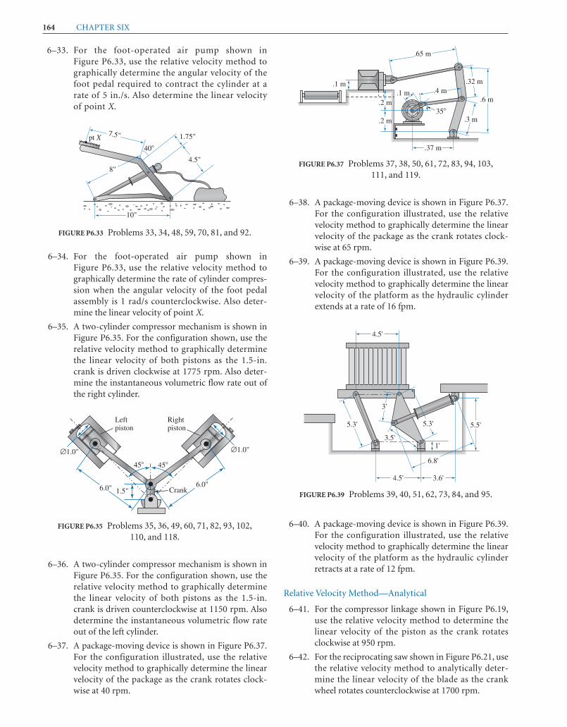
164 CHAPTER SIX
6–33. For the foot-operated air pump shown inFigure P6.33, use the relative velocity method tographically determine the angular velocity of thefoot pedal required to contract the cylinder at arate of 5 in./s. Also determine the linear velocityof point X.
6–38. A package-moving device is shown in Figure P6.37.For the configuration illustrated, use the relativevelocity method to graphically determine the linearvelocity of the package as the crank rotates clock-wise at 65 rpm.
6–39. A package-moving device is shown in Figure P6.39.For the configuration illustrated, use the relativevelocity method to graphically determine the linearvelocity of the platform as the hydraulic cylinderextends at a rate of 16 fpm.
7.5"pt X
40�
1.75"
4.5"
10"
8"
FIGURE P6.33 Problems 33, 34, 48, 59, 70, 81, and 92.
6–34. For the foot-operated air pump shown inFigure P6.33, use the relative velocity method tographically determine the rate of cylinder compres-sion when the angular velocity of the foot pedalassembly is 1 rad/s counterclockwise. Also deter-mine the linear velocity of point X.
6–35. A two-cylinder compressor mechanism is shown inFigure P6.35. For the configuration shown, use therelative velocity method to graphically determinethe linear velocity of both pistons as the 1.5-in.crank is driven clockwise at 1775 rpm. Also deter-mine the instantaneous volumetric flow rate out ofthe right cylinder.
Leftpiston
Rightpiston
∅1.0" ∅1.0"
6.0" 1.5"
45� 45�
Crank6.0"
FIGURE P6.35 Problems 35, 36, 49, 60, 71, 82, 93, 102,110, and 118.
6–36. A two-cylinder compressor mechanism is shown inFigure P6.35. For the configuration shown, use therelative velocity method to graphically determinethe linear velocity of both pistons as the 1.5-in.crank is driven counterclockwise at 1150 rpm. Alsodetermine the instantaneous volumetric flow rateout of the left cylinder.
6–37. A package-moving device is shown in Figure P6.37.For the configuration illustrated, use the relativevelocity method to graphically determine the linearvelocity of the package as the crank rotates clock-wise at 40 rpm.
.2 m
.2 m
.37 m
35�
.6 m
.3 m
.32 m
.65 m
.4 m.1 m.1 m
FIGURE P6.37 Problems 37, 38, 50, 61, 72, 83, 94, 103,111, and 119.
1'
5.3'
4.5'
3.6'
6.8'
4.5'
3.5'
5.3'
3'
5.5'
FIGURE P6.39 Problems 39, 40, 51, 62, 73, 84, and 95.
6–40. A package-moving device is shown in Figure P6.39.For the configuration illustrated, use the relativevelocity method to graphically determine the linearvelocity of the platform as the hydraulic cylinderretracts at a rate of 12 fpm.
Relative Velocity Method—Analytical
6–41. For the compressor linkage shown in Figure P6.19,use the relative velocity method to determine thelinear velocity of the piston as the crank rotatesclockwise at 950 rpm.
6–42. For the reciprocating saw shown in Figure P6.21, usethe relative velocity method to analytically deter-mine the linear velocity of the blade as the crankwheel rotates counterclockwise at 1700 rpm.

Velocity Analysis 165
6–43. For the shearing mechanism in the configurationshown in Figure P6.23, use the relative velocitymethod to analytically determine the linear velocityof the blade as the crank rotates clockwise at 85 rpm.
6–44. For the rear windshield wiper mechanism shown inFigure P6.25, use the relative velocity method toanalytically determine the angular velocity of thewiper arm as the crank rotates counterclockwise at45 rpm.
6–45. The device in Figure P6.27 is a sloshing bath used towash vegetable produce. For the configurationshown, use the relative velocity method to analyti-cally determine the angular velocity of the water bathas the crank is driven counterclockwise at 90 rpm.
6–46. The device in Figure P6.29 is a drive mechanism forthe agitator on a washing machine. For the configura-tion shown, use the relative velocity method to analyt-ically determine the angular velocity of the segmentgear as the crank is driven clockwise at 60 rpm.
6–47. For the links for the hand-operated shear shown inFigure P6.31, use the relative velocity method toanalytically determine the angular velocity of thehandle required to have the blade cut through themetal at a rate of 2 mm/s.
6–48. For the foot-operated air pump shown in FigureP6.33, use the relative velocity method to analyti-cally determine the rate of cylinder compression asthe foot pedal assembly rotates counterclockwise ata rate of 1 rad/s.
6–49. A two-cylinder compressor mechanism is shown inFigure P6.35. For the configuration shown, use therelative velocity method to analytically determinethe linear velocity of both pistons as the 1.5-in.crank is driven clockwise at 2000 rpm. Also deter-mine the instantaneous volumetric flow rate out ofthe right cylinder.
6–50. A package-moving device is shown in Figure P6.37.For the configuration illustrated, use the relativevelocity method to analytically determine the linearvelocity of the package as the crank rotates clock-wise at 80 rpm.
6–51. A package-moving device is shown in Figure P6.39.For the configuration illustrated, use the relativevelocity method to analytically determine the linearvelocity of the platform as the hydraulic cylinderretracts at a rate of 10 fpm.
Locating Instantaneous
Centers—Graphically
6–52. For the compressor linkage shown in Figure P6.19,graphically determine the location of all the instan-taneous centers.
6–53. For the reciprocating saw shown in Figure P6.21,graphically determine the location of all the instan-taneous centers.
6–54. For the shearing mechanism in the configurationshown in Figure P6.23, graphically determine thelocation of all the instantaneous centers.
6–55. For the rear windshield wiper mechanism shown inFigure P6.25, graphically determine the location ofall the instantaneous centers.
6–56. For the produce-washing bath shown in FigureP6.27, graphically determine the location of all theinstantaneous centers.
6–57. For the washing machine agitation mechanismshown in Figure P6.29, graphically determine thelocation of all the instantaneous centers.
6–58. For the hand-operated shear shown in Figure P6.31,graphically determine the location of all the instan-taneous centers.
6–59. For the foot-operated air pump shown in FigureP6.33, graphically determine the location of all theinstantaneous centers.
6–60. For the two-cylinder compressor mechanism shownin Figure P6.35, graphically determine the locationof all the instantaneous centers.
6–61. For the package-moving device shown in FigureP6.37, graphically determine the location of all theinstantaneous centers.
6–62. For the package-moving device shown in FigureP6.39, graphically determine the location of all theinstantaneous centers.
Locating Instantaneous
Centers—Analytically
6–63. For the compressor linkage shown in Figure P6.19,analytically determine the location of all the instan-taneous centers.
6–64. For the reciprocating saw shown in Figure P6.21,analytically determine the location of all the instan-taneous centers.
6–65. For the shearing mechanism in the configurationshown in Figure P6.23, analytically determine thelocation of all the instantaneous centers.
6–66. For the rear windshield wiper mechanism shown inFigure P6.25, analytically determine the location ofall the instantaneous centers.
6–67. For the produce-washing bath shown in FigureP6.27, analytically determine the location of all theinstantaneous centers.
6–68. For the washing machine agitation mechanismshown in Figure P6.29, analytically determine thelocation of all the instantaneous centers.
6–69. For the hand-operated shear shown in Figure P6.31,analytically determine the location of all the instan-taneous centers.
6–70. For the foot-operated air pump shown in FigureP6.33, analytically determine the location of all theinstantaneous centers.
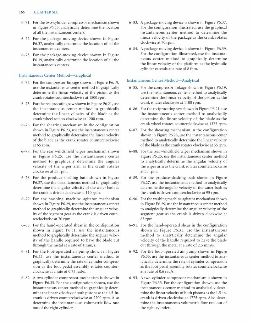
166 CHAPTER SIX
6–71. For the two-cylinder compressor mechanism shownin Figure P6.35, analytically determine the locationof all the instantaneous centers.
6–72. For the package-moving device shown in FigureP6.37, analytically determine the location of all theinstantaneous centers.
6–73. For the package-moving device shown in FigureP6.39, analytically determine the location of all theinstantaneous centers.
Instantaneous Center Method—Graphical
6–74. For the compressor linkage shown in Figure P6.19,use the instantaneous center method to graphicallydetermine the linear velocity of the piston as thecrank rotates counterclockwise at 1500 rpm.
6–75. For the reciprocating saw shown in Figure P6.21, usethe instantaneous center method to graphicallydetermine the linear velocity of the blade as thecrank wheel rotates clockwise at 1200 rpm.
6–76. For the shearing mechanism in the configurationshown in Figure P6.23, use the instantaneous centermethod to graphically determine the linear velocityof the blade as the crank rotates counterclockwiseat 65 rpm.
6–77. For the rear windshield wiper mechanism shownin Figure P6.25, use the instantaneous centermethod to graphically determine the angularvelocity of the wiper arm as the crank rotatesclockwise at 55 rpm.
6–78. For the produce-sloshing bath shown in FigureP6.27, use the instantaneous method to graphicallydetermine the angular velocity of the water bath asthe crank is driven clockwise at 110 rpm.
6–79. For the washing machine agitator mechanismshown in Figure P6.29, use the instantaneous centermethod to graphically determine the angular veloc-ity of the segment gear as the crank is driven coun-terclockwise at 70 rpm.
6–80. For the hand-operated shear in the configurationshown in Figure P6.31, use the instantaneousmethod to graphically determine the angular veloc-ity of the handle required to have the blade cutthrough the metal at a rate of 4 mm/s.
6–81. For the foot-operated air pump shown in FigureP6.33, use the instantaneous center method tographically determine the rate of cylinder compres-sion as the foot pedal assembly rotates counter-clockwise at a rate of 0.75 rad/s.
6–82. A two-cylinder compressor mechanism is shown inFigure P6.35. For the configuration shown, use theinstantaneous center method to graphically deter-mine the linear velocity of both pistons as the 1.5-in.crank is driven counterclockwise at 2200 rpm. Alsodetermine the instantaneous volumetric flow rateout of the right cylinder.
6–83. A package-moving device is shown in Figure P6.37.For the configuration illustrated, use the graphicalinstantaneous center method to determine thelinear velocity of the package as the crank rotatesclockwise at 70 rpm.
6–84. A package-moving device is shown in Figure P6.39.For the configuration illustrated, use the instanta-neous center method to graphically determinethe linear velocity of the platform as the hydrauliccylinder extends at a rate of 8 fpm.
Instantaneous Center Method—Analytical
6–85. For the compressor linkage shown in Figure P6.19,use the instantaneous center method to analyticallydetermine the linear velocity of the piston as thecrank rotates clockwise at 1100 rpm.
6–86. For the reciprocating saw shown in Figure P6.21, usethe instantaneous center method to analyticallydetermine the linear velocity of the blade as thecrank wheel rotates counterclockwise at 1375 rpm.
6–87. For the shearing mechanism in the configurationshown in Figure P6.23, use the instantaneous centermethod to analytically determine the linear velocityof the blade as the crank rotates clockwise at 55 rpm.
6–88. For the rear windshield wiper mechanism shown inFigure P6.25, use the instantaneous center methodto analytically determine the angular velocity ofthe wiper arm as the crank rotates counterclockwiseat 35 rpm.
6–89. For the produce-sloshing bath shown in FigureP6.27, use the instantaneous method to analyticallydetermine the angular velocity of the water bath asthe crank is driven counterclockwise at 95 rpm.
6–90. For the washing machine agitator mechanism shownin Figure P6.29, use the instantaneous center methodto analytically determine the angular velocity of thesegment gear as the crank is driven clockwise at85 rpm.
6–91. For the hand-operated shear in the configurationshown in Figure P6.31, use the instantaneousmethod to analytically determine the angularvelocity of the handle required to have the bladecut through the metal at a rate of 2.5 mm/s.
6–92. For the foot-operated air pump shown in FigureP6.33, use the instantaneous center method to ana-lytically determine the rate of cylinder compressionas the foot pedal assembly rotates counterclockwiseat a rate of 0.6 rad/s.
6–93. A two-cylinder compressor mechanism is shown inFigure P6.35. For the configuration shown, use theinstantaneous center method to analytically deter-mine the linear velocity of both pistons as the 1.5-in.crank is driven clockwise at 1775 rpm. Also deter-mine the instantaneous volumetric flow rate out ofthe right cylinder.

Velocity Analysis 167
6–94. A package-moving device is shown in Figure P6.37.For the configuration illustrated, use the graphicalinstantaneous center method to determine thelinear velocity of the package as the crank rotatesclockwise at 30 rpm.
6–95. A package-moving device is shown in Figure P6.39.For the configuration illustrated, use the instanta-neous center method to analytically determine thelinear velocity of the platform as the hydrauliccylinder retracts at a rate of 7 fpm.
Velocity Curves––Graphical
6–96. The crank of the compressor linkage shown inFigure P6.19 is driven clockwise at a constant rate of1750 rpm. Graphically create a curve for the lineardisplacement of the piston as a function of the crankangle. Convert the crank angle to time. Then graph-ically calculate the slope to obtain a velocity curve ofthe piston as a function of time.
6–97. The crank wheel of the reciprocating saw shownin Figure P6.21 is driven counterclockwise at aconstant rate of 1500 rpm. Graphically create acurve for the linear displacement of the saw bladeas a function of the crank angle. Convert the crankangle to time. Then graphically calculate the slopeto obtain a velocity curve of the saw blade as a func-tion of time.
6–98. The crank of the shearing mechanism shown inFigure P6.23 is driven clockwise at a constant rate of80 rpm. Graphically create a curve for the lineardisplacement of the shear blade as a function of thecrank angle. Convert the crank angle to time. Thengraphically calculate the slope to obtain a velocitycurve of the shear blade as a function of time.
6–99. The crank of the rear windshield wiper mechanismshown in Figure P6.25 is driven clockwise at aconstant rate of 65 rpm. Graphically create a curvefor the angular displacement of the wiper blade as afunction of the crank angle. Convert the crank angleto time. Then graphically calculate the slope toobtain an angular velocity curve of the wiper bladeas a function of time.
6–100. The crank of the sloshing bath shown in FigureP6.27 is driven counterclockwise at 90 rpm.Graphically create a curve for the angular displace-ment of the bath as a function of the crank angle.Convert the crank angle to time. Then graphicallycalculate the slope to obtain an angular velocitycurve of the bath as a function of time.
6–101. The crank of the washing machine agitator mecha-nism shown in Figure P6.29 is driven clockwise at80 rpm. Graphically create a curve for the angulardisplacement of the segment gear as a function of thecrank angle. Convert the crank angle to time. Thengraphically calculate the slope to obtain an angularvelocity of the segment gear as a function of time.
6–102. The crank of the two-cylinder compressor mecha-nism shown in Figure P6.35 is driven clockwise at1250 rpm. Graphically create a curve for the lineardisplacement of both pistons as a function of thecrank angle. Convert the crank angle to time. Thengraphically calculate the slope to obtain velocitycurves of both pistons as a function of time.
6–103. The crank of the package-moving device shown inFigure. P6.37 is driven clockwise at 25 rpm.Graphically create a curve for the linear displace-ment of the ram as a function of the crank angle.Convert the crank angle to time. Then graphicallycalculate the slope to obtain a velocity curve of theram as a function of time.
Velocity Curves—Analytical
6–104. The crank of the compressor linkage shown inFigure P6.19 is driven counterclockwise at a con-stant rate of 2150 rpm. Use a spreadsheet to analyti-cally create a curve for the linear displacement of thepiston as a function of the crank angle. Convert thecrank angle axis to time. Then use numerical differ-entiation to obtain a velocity curve of the piston as afunction of time.
6–105. The crank wheel of the reciprocating saw shown inFigure P6.21 is driven clockwise at a constant rate of1900 rpm. Use a spreadsheet to analytically create acurve for the linear displacement of the saw blade asa function of the crank angle. Convert the crankangle axis to time. Then use numerical differentia-tion to obtain a velocity curve of the saw blade as afunction of time.
6–106. The crank of the shearing mechanism shown inFigure P6.23 is driven clockwise at a constant rate of80 rpm. Use a spreadsheet to analytically create acurve for the linear displacement of the shear bladeas a function of the crank angle. Convert the crankangle axis to time. Then use numerical differentia-tion to obtain a velocity curve of the shear blade as afunction of time.
6–107. The crank of the rear windshield wiper mecha-nism shown in Figure P6.25 is driven counter-clockwise at a constant rate of 55 rpm. Use aspreadsheet to analytically create a curve for theangular displacement of the wiper blade as a func-tion of the crank angle. Convert the crank angleaxis to time. Then use numerical differentiation toobtain an angular velocity curve of the wiperblade as a function of time.
6–108. The crank of the sloshing bath shown in FigureP6.27 is driven clockwise at 65 rpm. Use a spread-sheet to analytically create a curve for the angulardisplacement of the bath as a function of the crankangle. Convert the crank angle axis to time. Thenuse numerical differentiation to obtain an angularvelocity curve of the bath as a function of time.

168 CHAPTER SIX
6–109. The crank of the washing machine agitator mecha-nism shown in Figure P6.29 is driven counterclock-wise at 65 rpm. Use a spreadsheet to analyticallycreate a curve for the angular displacement of thesegment gear as a function of the crank angle.Convert the crank angle axis to time. Then usenumerical differentiation to obtain an angular veloc-ity curve of the segment gear as a function of time.
6–110. The crank of the two-cylinder compressor mecha-nism shown in Figure P6.35 is driven counterclock-wise at 1500 rpm. Use a spreadsheet to analyticallycreate a curve for the linear displacement of bothpistons as a function of the crank angle. Convertthe crank angle axis to time. Then use numericaldifferentiation to obtain velocity curves of bothpistons as a function of time.
6–111. The crank of the package-moving device shown inFigure P6.37 is driven counterclockwise at 30 rpm.Use a spreadsheet to analytically create a curve forthe linear displacement of the ram as a function ofthe crank angle. Convert the crank angle axis totime. Then use numerical differentiation to obtain avelocity curve of the ram as a function of time.
Velocity Using Working Model
6–112. The crank of the compressor linkage shown inFigure P6.19 is driven clockwise at a constant rateof 1750 rpm. Use the Working Model software tocreate a simulation and plot the linear velocity of thepiston as a function of the crank angle.
6–113. The crank wheel of the reciprocating saw shownin Figure P6.21 is driven counterclockwise at aconstant rate of 1500 rpm. Use the Working Modelsoftware to create a simulation and plot the linearvelocity of the saw blade as a function of the crankangle.
6–114. The crank of the shearing mechanism shown inFigure P6.23 is driven clockwise at a constant rate of80 rpm. Use the Working Model software to create asimulation and plot the angular velocity of thewiper blade as a function of the crank angle.
6–115. The crank of the rear windshield wiper mechanismshown in Figure P6.25 is driven clockwise at a con-stant rate of 65 rpm. Use the Working Model softwareto create a simulation and plot the angular velocity ofthe wiper blade as a function of the crank angle.
6–116. The crank of the sloshing bath shown in FigureP6.27 is driven counterclockwise at 90 rpm. Use theWorking Model software to create a simulation andplot the angular velocity of the bath as a function ofthe crank angle.
6–117. The crank of the washing machine agitator mecha-nism shown in Figure P6.29 is driven clockwise at80 rpm. Use the Working Model software to create asimulation and plot the angular velocity of thesegment gear as a function of the crank angle.
6–118. The crank of the two-cylinder compressor mecha-nism shown in Figure P6.35 is driven clockwiseat 1250 rpm. Use the Working Model software tocreate a simulation and plot the angular velocity ofboth pistons as a function of the crank angle.
6–119. The crank of the package-moving device shown inFigure P6.37 is driven clockwise at 25 rpm. Use theWorking Model software to create a simulation andplot the linear velocity of the ram as a function ofthe crank angle.
CASE STUDIES
6–1. Figure C6.1 illustrates a mechanism that is used todrive a power hacksaw. The mechanism is poweredwith an electric motor shaft, keyed to gear A.Carefully examine the configuration in question,then answer the following leading questions to gaininsight into the operation of the mechanism.
E
B
A
CD
FIGURE C6.1 (Courtesy, Industrial Press.)
1. When gear A is forced to rotate counterclockwise,what is the motion of mating gear B ?
2. When gear A is forced to rotate counterclockwise,what is the motion of stud pin C ?
3. When gear A is forced to rotate counterclockwise,what is the motion of lever D?
4. How does the motion of lever D differ from themotion of lever E ?
5. Determine the position of gear B that would placelever D at its lower extreme position.
6. Determine the position of gear B that would placelever D at its upper extreme position.
7. Examine the amount of rotation of gear B to raiselever D and the amount of rotation to lower thelever.
8. Approximately what is the difference between thetime to raise and the time to lower lever D?
9. Comment on the continual motion of lever E.

Velocity Analysis 169
6–2. Figure C6.2 illustrates the mechanism that drives atable for a special grinding operation. Carefullyexamine the configuration in question, then answerthe following leading questions to gain insight intothe operation of the mechanism.
6–3. Figure C6.3 illustrates the mechanism that drives abellows for an artificial respiration machine.Carefully examine the configuration in question,then answer the following leading questions to gaininsight into the operation of the mechanism.
N
H
A
R
B C
JF D G
I
FIGURE C6.2 (Courtesy, Industrial Press.)
1. When wheel C is forced to rotate counterclockwise,what is the motion of pin D?
2. When wheel C is forced to rotate counterclockwise,what is the motion of link G ?
3. Determine the position of wheel C that would placepoint I at its upper extreme position.
4. Determine the position of wheel C that would placepoint I at its lower extreme position.
5. Examine the amount of rotation of wheel C to raisepoint I and the amount of rotation to lower thepoint.
6. Approximately what is the difference between thetime to raise and the time to lower point I ?
7. Comment on the cyclical motion of lever E.8. Describe the motion of table R.9. What is the function of this mechanism?
10. Why are there screw threads on both ends of link H ?11. Compute the mobility of this mechanism.
1. When link E drives continually counterclockwiseand rides slot J, at the instant shown, what is themotion of disk F ?
2. When link E drives continually counterclockwiseand rides slot J, at the instant shown, what is themotion of strap G ?
3. When link E drives continually counterclockwiseand rides slot J, at the instant shown, what is themotion of slide A?
4. As link E approaches the ramped pad M, whathappens to the spring N ?
5. As link E contacts the ramped pad M, what happensto link E ?
6. As link E contacts the ramped pad M, what is themotion of disk F ?
7. As link E contacts the ramped pad M, what is themotion of slide A?
8. As link E continues to rotate beyond the rampedpad M, what is the motion of disk F ?
9. As link E catches slot K, what is the motion of disk F ?10. Describe the continual motion of slide A, which
drives one end of the bellows.
M E BTop View
Front View
F P
C
G N
A
G
P
K
N
F
BE
H
LM
J
A
FIGURE C6.3 (Courtesy, Industrial Press.)

170
C H A P T E R
S E V E N
ACCELERATION ANALYSIS
analysis is the relative acceleration method, which utilizesthe results of the relative velocity method introduced inChapter 6. Consistent with other chapters in this book, bothgraphical and analytical techniques are utilized.
7.2 LINEAR ACCELERATION
Linear acceleration, A, of a point is the change of linearvelocity of that point per unit of time. Chapter 6 was dedi-cated to velocity analysis. Velocity is a vector quantity, whichis defined with both a magnitude and a direction. Therefore,a change in either the magnitude or direction of velocityproduces an acceleration. The magnitude of the accelerationvector is designated .
7.2.1 Linear Acceleration of RectilinearPoints
Consider the case of a point having straight line, or recti-linear, motion. Such a point is most commonly found on alink that is attached to the frame with a sliding joint. For thiscase, only the magnitude of the velocity vector can change.The acceleration can be mathematically described as
(7.1)
However, because
then
(7.2)
For short time periods, or when the acceleration can beassumed to be linear, the following relationship can be used:
(7.3)
Because velocity is a vector, equation (7.1) states thatacceleration is also a vector. The direction of linear accelerationis in the direction of linear movement when the link accelerates.Conversely, when the link decelerates, the direction of linearacceleration is opposite to the direction of linear movement.
A �¢V
¢t
A =d 2 R
dt 2
V =dR
dt
A = lim¢t:0
¢V
¢t=
dv
dt
a = ƒ A ƒ
O B J E C T I V E S
Upon completion of this chapter, the student will be able to:
1. Define linear, rotational, normal, tangential, Coriolis,and relative accelerations.
2. Use the relative acceleration method to graphicallysolve for the acceleration of a point on a link,knowing the acceleration of another point on that link.
3. Use the relative acceleration method to graphicallydetermine the acceleration of a point of interest on afloating link.
4. Understand when the Coriolis acceleration is present,and include it in the analysis.
5. Use the relative acceleration method to analyticallysolve for the acceleration of a point.
6. Use the relative acceleration method to analyticallydetermine the acceleration of a point of interest on afloating link.
7. Construct an acceleration curve to locate extremeacceleration values.
7.1 INTRODUCTION
Acceleration analysis involves determining the manner inwhich certain points on the links of a mechanism are either“speeding up” or “slowing down.” Acceleration is a criticalproperty because of the inertial forces associated with it. Inthe study of forces, Sir Isaac Newton discovered that an iner-tial force is proportional to the acceleration imposed on abody. This phenomenon is witnessed anytime you lungeforward as the brakes are forcefully applied on your car.
Of course, an important part of mechanism design is toensure that the strength of the links and joints is sufficient towithstand the forces imposed on them. Understanding allforces, especially inertia, is important. Force analysis isintroduced in Chapters 13 and 14. However, as a preliminarystep, acceleration analysis of a mechanism’s links must beperformed.
The determination of accelerations in a linkage is thepurpose of this chapter. The primary procedure used in this

Acceleration Analysis 171
Linear acceleration is expressed in the units of velocity(length per time) divided by time, or length per squared time.In the U.S. Customary System, the common units used arefeet per squared second (ft/s2) or inches per squared second(in./s2). In the International System, the common units usedare meters per squared second (m/s2) or millimeters persquared second (mm/s2). For comparison purposes, linearacceleration is often stated relative to the acceleration due togravity . Thus, a10g acceleration is equivalent to 3864 in./s2.
7.2.2 Constant Rectilinear Acceleration
Rewriting equation (7.3), the velocity change that occursduring a period of constant acceleration is expressed as
(7.4)¢V = Vfinal - Vinitial = A ¢t
g = 32.17 ft/s2 = 386.4 in./s2 = 9.81 m/s2
Additionally, the corresponding displacement thatoccurs during a period of constant acceleration can bewritten as
(7.5)
Equations (7.4) and (7.5) can be combined to give
(7.6)
Since rectilinear motion is along a straight line, the directionof the displacement, velocity, and acceleration (r, v, a) can bespecified with an algebraic sign along a coordinate axis.Thus, equations (7.4), (7.5), and (7.6) can be written interms of the vector magnitudes (r, v, a).
(Vfinal)2 = (Vinitial)
2 + 2 A ¢R
¢R =1
2A¢t2 + Vinitial ¢t
EXAMPLE PROBLEM 7.1
An express elevator used in tall buildings can reach a full speed of 15 mph in 3 s. Assuming that the elevator experiences
constant acceleration, determine the acceleration and the displacement during the 3 s.
SOLUTION: 1. Calculate Acceleration
Assuming that the acceleration is constant, equation (7.3) can be accurately used. Because the elevator starts at
rest, the velocity change is calculated as
Then, the acceleration is calculated as
2. Normalize the Acceleration with Respect to Gravity
When people accelerate in an elevator, the acceleration is often “normalized” relative to the acceleration due to
gravity. The standard acceleration due to gravity (g) on earth is 32.17 ft/s2 or 9.81 m/s2. Therefore, the accelera-
tion of the elevator can be expressed as
3. Calculate the Displacement during the 3-Second Interval
The displacement can be determined from equation (7.5).
= 32.9 ft c (or roughly 3 floors)
¢R =1
2a¢t 2 + vinitial¢t =
1
217.3 ft/s22(3 s)2 + (0)(3 s)
A = 7.3 ft/s2 a 1 g
32.2 ft/s2 b = 0.22 g
A =¢V
¢t=122 ft/s2
3 s= 7.3 ft / s2 c
= a 15 miles
hrb a 5280 ft
1 mileb a 1 hr
3600 sb = 22 ft/s
¢V = (15 mph - 0) = 15 mph
7.2.3 Acceleration and the Velocity Profile
As stated in equation (7.1), the instantaneous acceleration isthe first derivative of the instantaneous velocity with respectto time. Occasionally, a closed-form equation for the instan-taneous velocity of a point is available. In these cases, thederivative of the equation, evaluated at the specified time,
will yield the instantaneous acceleration. More often, espe-cially in programmable actuators used in automation,velocity profiles are specified as introduced in Chapter 6.Recall that the displacement for a certain time interval is thearea under the v-t curve for that time interval. Conversely,the acceleration at a certain time is the slope of the v-t curve.
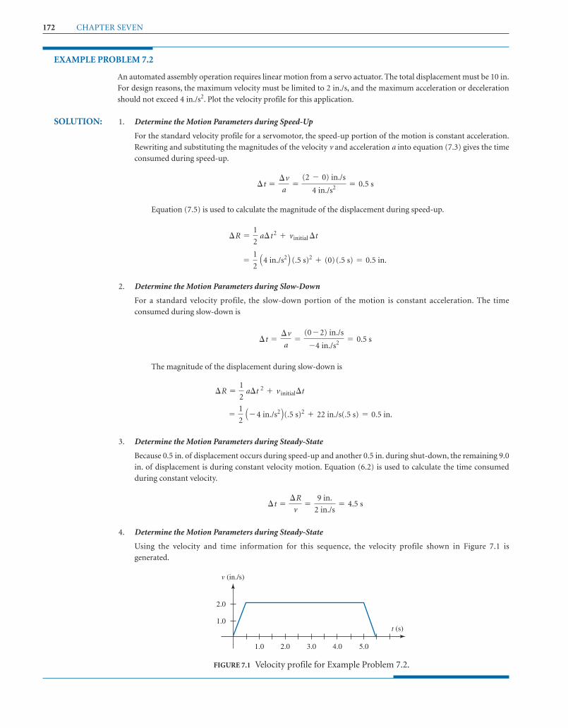
172 CHAPTER SEVEN
EXAMPLE PROBLEM 7.2
An automated assembly operation requires linear motion from a servo actuator. The total displacement must be 10 in.
For design reasons, the maximum velocity must be limited to 2 in./s, and the maximum acceleration or deceleration
should not exceed 4 in./s2. Plot the velocity profile for this application.
SOLUTION: 1. Determine the Motion Parameters during Speed-Up
For the standard velocity profile for a servomotor, the speed-up portion of the motion is constant acceleration.
Rewriting and substituting the magnitudes of the velocity v and acceleration a into equation (7.3) gives the time
consumed during speed-up.
Equation (7.5) is used to calculate the magnitude of the displacement during speed-up.
2. Determine the Motion Parameters during Slow-Down
For a standard velocity profile, the slow-down portion of the motion is constant acceleration. The time
consumed during slow-down is
The magnitude of the displacement during slow-down is
3. Determine the Motion Parameters during Steady-State
Because 0.5 in. of displacement occurs during speed-up and another 0.5 in. during shut-down, the remaining 9.0
in. of displacement is during constant velocity motion. Equation (6.2) is used to calculate the time consumed
during constant velocity.
4. Determine the Motion Parameters during Steady-State
Using the velocity and time information for this sequence, the velocity profile shown in Figure 7.1 is
generated.
¢t =¢R
v=
9 in.
2 in./s= 4.5 s
=1
2A - 4 in./s2 B(.5 s)2 + 22 in./s(.5 s) = 0.5 in.
¢R =1
2a¢t 2 + v initial¢t
¢t =¢v
a=
(0 - 2) in./s
-4 in./s2 = 0.5 s
=1
2A4 in./s2 B (.5 s)2 + (0)(.5 s) = 0.5 in.
¢R =1
2a¢t 2 + vinitial ¢t
¢t =¢v
a=
(2 - 0) in./s
4 in./s2 = 0.5 s
v (in./s)
t (s)
2.0
1.0
1.0 2.0 3.0 4.0 5.0
FIGURE 7.1 Velocity profile for Example Problem 7.2.
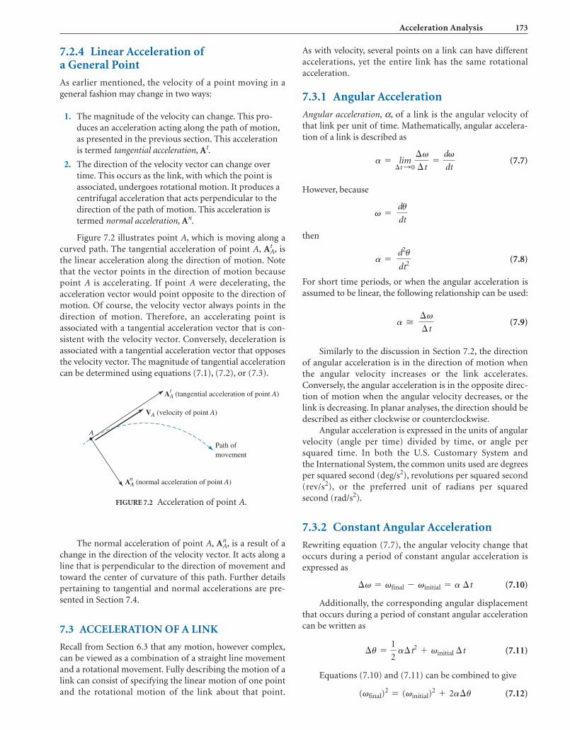
Acceleration Analysis 173
A
AA (normal acceleration of point A)n
AA (tangential acceleration of point A)t
Path ofmovement
VA (velocity of point A)
FIGURE 7.2 Acceleration of point A.
7.2.4 Linear Acceleration ofa General Point
As earlier mentioned, the velocity of a point moving in ageneral fashion may change in two ways:
1. The magnitude of the velocity can change. This pro-duces an acceleration acting along the path of motion,as presented in the previous section. This accelerationis termed tangential acceleration, At.
2. The direction of the velocity vector can change overtime. This occurs as the link, with which the point isassociated, undergoes rotational motion. It produces acentrifugal acceleration that acts perpendicular to thedirection of the path of motion. This acceleration istermed normal acceleration, An.
Figure 7.2 illustrates point A, which is moving along acurved path. The tangential acceleration of point A, , isthe linear acceleration along the direction of motion. Notethat the vector points in the direction of motion becausepoint A is accelerating. If point A were decelerating, theacceleration vector would point opposite to the direction ofmotion. Of course, the velocity vector always points in thedirection of motion. Therefore, an accelerating point isassociated with a tangential acceleration vector that is con-sistent with the velocity vector. Conversely, deceleration isassociated with a tangential acceleration vector that opposesthe velocity vector. The magnitude of tangential accelerationcan be determined using equations (7.1), (7.2), or (7.3).
AAt
As with velocity, several points on a link can have differentaccelerations, yet the entire link has the same rotationalacceleration.
7.3.1 Angular Acceleration
Angular acceleration, α, of a link is the angular velocity ofthat link per unit of time. Mathematically, angular accelera-tion of a link is described as
(7.7)
However, because
then
(7.8)
For short time periods, or when the angular acceleration isassumed to be linear, the following relationship can be used:
(7.9)
Similarly to the discussion in Section 7.2, the directionof angular acceleration is in the direction of motion whenthe angular velocity increases or the link accelerates.Conversely, the angular acceleration is in the opposite direc-tion of motion when the angular velocity decreases, or thelink is decreasing. In planar analyses, the direction should bedescribed as either clockwise or counterclockwise.
Angular acceleration is expressed in the units of angularvelocity (angle per time) divided by time, or angle persquared time. In both the U.S. Customary System andthe International System, the common units used are degreesper squared second (deg/s2), revolutions per squared second(rev/s2), or the preferred unit of radians per squaredsecond (rad/s2).
7.3.2 Constant Angular Acceleration
Rewriting equation (7.7), the angular velocity change thatoccurs during a period of constant angular acceleration isexpressed as
(7.10)
Additionally, the corresponding angular displacementthat occurs during a period of constant angular accelerationcan be written as
(7.11)
Equations (7.10) and (7.11) can be combined to give
(7.12)(vfinal)2 = (vinitial)
2 + 2a¢u
¢u =1
2a¢t2 + vinitial ¢t
¢v = vfinal - vinitial = a ¢t
a �¢v¢t
a =d2u
dt2
v =du
dt
a = lim¢t:0
¢v¢t
=dv
dt
The normal acceleration of point A, , is a result of achange in the direction of the velocity vector. It acts along aline that is perpendicular to the direction of movement andtoward the center of curvature of this path. Further detailspertaining to tangential and normal accelerations are pre-sented in Section 7.4.
7.3 ACCELERATION OF A LINK
Recall from Section 6.3 that any motion, however complex,can be viewed as a combination of a straight line movementand a rotational movement. Fully describing the motion of alink can consist of specifying the linear motion of one pointand the rotational motion of the link about that point.
AAn

174 CHAPTER SEVEN
ω α
FIGURE 7.3 Grinding wheel for Example Problem 7.3.
EXAMPLE PROBLEM 7.3
An electric motor drives the grinding wheel clockwise, as shown in Figure 7.3. It will speed up to 1800 rpm in 2 s
when the power is turned on. Assuming that this speed-up is at a constant rate, determine the angular
acceleration of the grinding wheel. Also determine the number of revolutions that the wheel spins before it is at
full speed.
SOLUTION: 1. Calculate the Acceleration
Since acceleration is typically specified in rad/s2, convert the speed of the grinding wheel to rad/s with the fol-
lowing:
With constant acceleration, equation (7.9) can be used, giving
The direction of the acceleration is clockwise, which is in the direction of motion because the grinding
wheel is speeding up.
2. Calculate the Displacement during the 2-Second Interval
The number of revolutions during this speed-up period can be determined through equation (7.11).
= 188.4 rada 1 rev
2p radb = 30.0 revolutions
¢u =1
2a¢t2 + vinitial¢t =
1
2A94.2 rad/s2 B(2 s)2 + (0)(2 s)
= a 188.5 rad/s - 0
2 sb = 94.2 rad/s2, cw
a =¢v¢t
¢v = 1800 rpma 2p rad
1 revb a 1 min
60 sb = 188.5 rad/s, cw
7.4 NORMAL AND TANGENTIALACCELERATION
As presented in Section 7.2.4, the velocity of a point mov-ing in a general path can change in two independent ways.The magnitude or the direction of the velocity vector canchange over time. Of course, acceleration is the time rate ofvelocity change. Thus, acceleration is commonly separatedinto two elements: normal and tangential components. Thenormal component is created as a result of a change in thedirection of the velocity vector. The tangential component
is formed as a result of a change in the magnitude of thevelocity vector.
7.4.1 Tangential Acceleration
For a point on a rotating link, little effort is required todetermine the direction of these acceleration compo-nents. Recall that the instantaneous velocity of a point ona rotating link is perpendicular to a line that connects thatpoint to the center of rotation. Any change in the magni-tude of this velocity creates tangential acceleration, which

Acceleration Analysis 175
2
0
A
(a) (b)
dθ2
dθ2dV
O
dV = VA″ – > VA′
rA
VA′
VA′
VA″
VA″
FIGURE 7.4 Normal acceleration.
is also perpendicular to the line that connects the pointwith the center of rotation. The magnitude of the tan-gential acceleration of point A on a rotating link 2 can beexpressed as
(7.13)
It is extremely important to remember that the angularacceleration, α, in equation (7.13) must be expressed as unitsof radians per squared time. Radians per squared second isthe most common unit. Similarly to the discussion inSection 7.2, tangential acceleration acts in the direction ofmotion when the velocity increases or the point accelerates.Conversely, tangential acceleration acts in the oppositedirection of motion when the velocity decreases or the pointdecelerates.
7.4.2 Normal Acceleration
Any change in velocity direction creates normal accele-ration, which is always directed toward the center ofrotation. Figure 7.4a illustrates a link rotating at constantspeed. The velocity of point A is shown slightly before andafter the configuration under consideration, separated by asmall angle dθ2. Because the link is rotating at constantspeed, the magnitudes of are equal. Thus,
.Figure 7.4b shows a velocity polygon, vectorally solving
for the change in velocity, dv. Notice that the change of thevelocity vector, dv, is directed toward the center of link rota-tion. In fact, the normal acceleration will always be directedtoward the center of link rotation. This is because, as thepoint rotates around a fixed pivot, the velocity vector willchange along the curvature of motion. Thus, the normal
VA¿ = VA–VA¿ and VA–
aAt =
dvA
dt=
d(v2rOA)
dt= rOA
dv2
dt= rOAa2
vector to this curvature will always be directed toward thefixed pivot.
In Figure 7.4a, because Δ is small, the followingrelationship can be stated:
Because acceleration is defined as the time rate of velocitychange, both sides should be divided by time:
Using equation (6.6), the relationships between the magni-tude of the linear velocity and angular velocity, the followingequations for the magnitude of the normal acceleration of apoint can be derived:
(7.14)
(7.15)
7.4.3 Total Acceleration
As previously mentioned, acceleration analysis is importantbecause inertial forces result from accelerations. These loadsmust be determined to ensure that the machine isadequately designed to handle these dynamic loads. Inertialforces are proportional to the total acceleration of a body.The total acceleration, A, is the vector resultant of thetangential and normal components. Mathematically, it isexpressed as
(7.16)AA = AAn +7 AA
t
aAn = vAv2 = vAa vA
rOAb =
vA2
rOA
aAn = vAv2 = (v2rOA)v2 = v2
2 rOA
aAn =
dvA
dt= vA
du2
dt= vAv2
dvA = vAdu2
u
EXAMPLE PROBLEM 7.4
The mechanism shown in Figure 7.5 is used in a distribution center to push boxes along a platform and to a loading
area. The input link is driven by an electric motor, which, at the instant shown, has a velocity of 25 rad/s and
accelerates at a rate of 500 rad/s2. Knowing that the input link has a length of 250 mm, determine the instantaneous
acceleration of the end of the input link in the position shown.
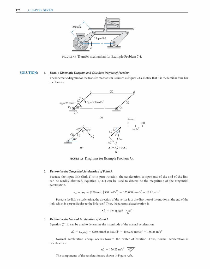
176 CHAPTER SEVEN
40°
ω
Input link
250 mm
FIGURE 7.5 Transfer mechanism for Example Problem 7.4.
40°
40°
40°
40°50°90°
1
2 = 500 rad/s2αω
β
2 = 25 rad/s
O2 O4
(a)
(b)
(c)
BA 3
2
A
2
4
AAtAA
n
AAt
AA
AA
n
0
Scale:
mm/s2
100
AA = AA + > AAtn
FIGURE 7.6 Diagrams for Example Problem 7.4.
SOLUTION: 1. Draw a Kinematic Diagram and Calculate Degrees of Freedom
The kinematic diagram for the transfer mechanism is shown as Figure 7.6a. Notice that it is the familiar four-bar
mechanism.
2. Determine the Tangential Acceleration of Point A
Because the input link (link 2) is in pure rotation, the acceleration components of the end of the link
can be readily obtained. Equation (7.13) can be used to determine the magnitude of the tangential
acceleration.
Because the link is accelerating, the direction of the vector is in the direction of the motion at the end of the
link, which is perpendicular to the link itself. Thus, the tangential acceleration is
3. Determine the Normal Acceleration of Point A
Equation (7.14) can be used to determine the magnitude of the normal acceleration.
Normal acceleration always occurs toward the center of rotation. Thus, normal acceleration is
calculated as
The components of the acceleration are shown in Figure 7.6b.
AAn = 156.25 m/s2 40°
aAn = rO2Av2
2 = (250 mm) A25 rad/s B2 = 156,250 mm/s2 = 156.25 m/s2
A At = 125.0 m/s2 50°
aAt = ra2 = (250 mm) A500 rad/s2 B = 125,000 mm/s2 = 125.0 m/s2
R
b
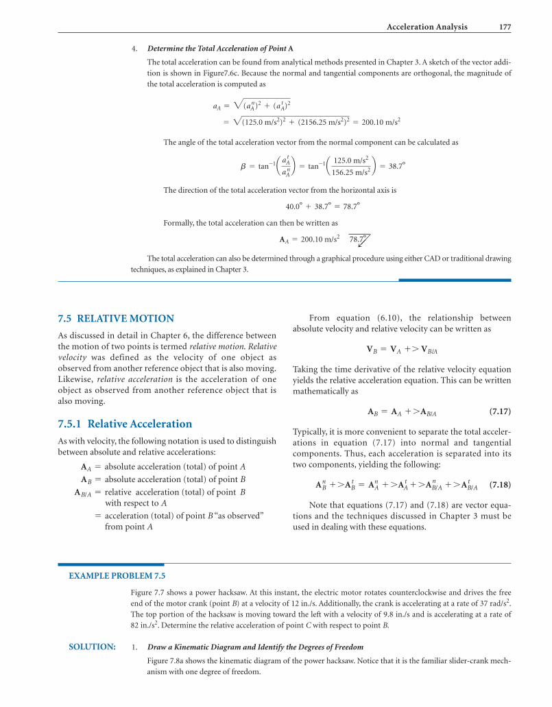
Acceleration Analysis 177
4. Determine the Total Acceleration of Point A
The total acceleration can be found from analytical methods presented in Chapter 3. A sketch of the vector addi-
tion is shown in Figure7.6c. Because the normal and tangential components are orthogonal, the magnitude of
the total acceleration is computed as
The angle of the total acceleration vector from the normal component can be calculated as
The direction of the total acceleration vector from the horizontal axis is
Formally, the total acceleration can then be written as
The total acceleration can also be determined through a graphical procedure using either CAD or traditional drawing
techniques, as explained in Chapter 3.
AA = 200.10 m/s2 78.7°
40.0° + 38.7° = 78.7°
b = tan-1a aAt
aAn b = tan-1a 125.0 m/s2
156.25 m/s2 b = 38.7°
= 2(125.0 m/s2)2 + (2156.25 m/s2)2 = 200.10 m/s2
aA = 3(aAn)2 + (aA
t )2
7.5 RELATIVE MOTION
As discussed in detail in Chapter 6, the difference betweenthe motion of two points is termed relative motion. Relativevelocity was defined as the velocity of one object asobserved from another reference object that is also moving.Likewise, relative acceleration is the acceleration of oneobject as observed from another reference object that isalso moving.
7.5.1 Relative Acceleration
As with velocity, the following notation is used to distinguishbetween absolute and relative accelerations:
“as observed”from point A
= acceleration (total) of point B
with respect to AAB/A = relative acceleration (total) of point B
AB = absolute acceleration (total) of point B
AA = absolute acceleration (total) of point A
From equation (6.10), the relationship betweenabsolute velocity and relative velocity can be written as
Taking the time derivative of the relative velocity equationyields the relative acceleration equation. This can be writtenmathematically as
(7.17)
Typically, it is more convenient to separate the total acceler-ations in equation (7.17) into normal and tangentialcomponents. Thus, each acceleration is separated into itstwo components, yielding the following:
(7.18)
Note that equations (7.17) and (7.18) are vector equa-tions and the techniques discussed in Chapter 3 must beused in dealing with these equations.
ABn + 7AB
t = AAn + 7AA
t + 7AB/An + 7 AB/A
t
AB = AA + 7AB/A
VB = VA + 7 VB/A
EXAMPLE PROBLEM 7.5
Figure 7.7 shows a power hacksaw. At this instant, the electric motor rotates counterclockwise and drives the free
end of the motor crank (point B) at a velocity of 12 in./s. Additionally, the crank is accelerating at a rate of 37 rad/s2.
The top portion of the hacksaw is moving toward the left with a velocity of 9.8 in./s and is accelerating at a rate of
82 in./s2. Determine the relative acceleration of point C with respect to point B.
SOLUTION: 1. Draw a Kinematic Diagram and Identify the Degrees of Freedom
Figure 7.8a shows the kinematic diagram of the power hacksaw. Notice that it is the familiar slider-crank mech-
anism with one degree of freedom.
b

178 CHAPTER SEVEN
30°
15° C
B
6.0''
1.75''
FIGURE 7.7 Power saw for Example Problem 7.5.
30°
30°
60°B
2
2α
ω
(a)
(c)
(b)
C
21.75"
1.75"
415°
B
AA1
3
6"
2
1
30°AB
AB
AC AC/B
AC/B = AC – > – >
n
n
ABt
ABtAB
n
ABt
........
FIGURE 7.8 Kinematic diagram for Example Problem 7.5.
2. Determine the Tangential Acceleration of Point B
From the kinematic diagram, it should be apparent that point B travels up and to the left as link 2 rotates coun-
terclockwise. Because the motor crank (link 2) is in pure rotation, the components of the acceleration at the end
of the link can be readily obtained. Equation (7.13) can be used to determine the magnitude of the tangential ac-
celeration.
Because the link accelerates, the direction of the vector is in the direction of the motion at the end of the
link. Thus, the tangential acceleration is calculated as
3. Determine the Normal Acceleration of Point B
Equation (7.15) can be used to determine the magnitude of the normal acceleration.
Normal acceleration is always directed toward the center of rotation. Thus, normal acceleration is
Link 2 is isolated and the components of this acceleration are shown in Figure 7.8b.
4. Specify the Acceleration of Point C
Point C is constrained to linear motion. Therefore, point C does not experience a normal acceleration. The total
acceleration is given in the problem statement as
AC = 82 in./s2 ;
ABn = 82.29 in./s2 30°
aBn = v
2B
rAB=112 in./s22
1.75 in.= 82.29 in./s2
ABt = 64.75 in./s2 60°
aBt = rABa2 = (1.75 in.) A37 rad/s2 B = 64.75 in./s2
a
b

Acceleration Analysis 179
5. Construct the Velocity Polygon for the Acceleration of C Relative to B
To determine the relative acceleration, equation (7.16) can be written in terms of points B and C and
rearranged as
Because two acceleration components of point B exist, the equation is written as
A vector polygon is formed from this equation (Figure 7.8c). The unknown vector can be determined
using the methods presented in Chapter 3. Either a graphical or analytical solution can be used to determine
vector AC/B.
6. Solve for the Unknown Vector Magnitudes
Arbitrarily using an analytical method, the acceleration AC/B can be found by separating the vectors into
horizontal and vertical components. See Table 7.1.
AC/B = AC - 71ABn + 7 AB
t2 = AC - 7 ABn - 7 AB
t
AC/B = AC - 7 AB
7.5.2 Components of Relative Acceleration
The acceleration of points on a mechanism can be muchmore easily analyzed when separated into normal andtangential components. For links that are attached directlyto the frame, the direction of the acceleration componentsis obvious, as described in the previous section. Thenormal component is always directed to the center of rota-tion, and the tangential component is perpendicular to thenormal component and in the direction that is consistent
with either the acceleration or deceleration of the point.Recall that tangential acceleration is in the direction ofmotion when the point accelerates. Conversely, tangentialacceleration is opposite to the direction of motion whenthe point decelerates.
For points that are on the same link, a link that is notdirectly attached to the frame, the analysis focuses on therelative accelerations of these points. Figure 7.9 shows such alink that is not directly attached to the frame, typically called
Separate algebraic equations can be written for the horizontal and vertical components as follows:
vertical comp.:
The magnitude of the acceleration can be found by
The direction of the vector can be determined by
Finally, the relative acceleration of C with respect to B is
AC/B = 26.05 in./s2 35°
ux = tan-1 c ahC/B
avC/Bd = tan-1 c -14.93 in./s2
21.35 in./s2 d = -35° = 35°
= 2(21.35)2 + (-14.93)2 = 26.05 in./s2
AC/B = 3Aa hC/B B2 + Aa v
C/B B2
Av C /B = (0) - (-41.15) - (+56.08) = -14.93 in./s2
= + 21.35 = 21.35 in./s2
horizontal comp.: AhC/B = (-82.0) - (-71.27) - (-32.38)
AC/B = AC - 7 ABn - 7 AB
t
TABLE 7.1 Horizontal and Vertical Vector Components for Acceleration AC/B
Vector Reference Angle ( )U x
Horizontal Component ah = a cos U x
Vertical Component av = a sin Ux
Ac 180° - 82.00 0
ABn 210° - 71.26 - 41.15
ABt 120° - 32.83 56.08
R
R

180 CHAPTER SEVEN
AB/A
B
A
AB/An
AB/At
FIGURE 7.9 Relative normal and tangential accelerations.
a floating link. The relative acceleration between two pointsthat reside on that link is shown. Notice that the normal andtangential components of this acceleration are also shownand are directed along the link (normal) and perpendicularto the link (tangential). Reiterating, the relative accelerationof two points is the acceleration of one point as seen fromthe other reference point.
As with velocity analysis, relative motion consists ofpure relative rotation of the observed point about the
reference point. In other terms, the relative motion of B withrespect to A is visualized as if point B were rotating aroundpoint A. Thus, a normal component of relative accelerationis directed toward the center of relative rotation, or the refer-ence point. The tangential relative acceleration is directedperpendicular to the normal relative acceleration. Themagnitudes of these components are computed in a similarfashion to the absolute acceleration of points rotatingaround fixed points.
(7.19)
(7.20)
The direction of the relative tangential acceleration isconsistent with the angular acceleration of the floatinglink, and vice versa. Referring to Figure 7.9, the relativetangential acceleration shows the tangential acceleration ofpoint B as it rotates around point A directed upward andtoward the right, which infers a clockwise angular accele-ration of link 3.
aB/An = rBAv
2 =(vB/A)2
rBA
aB/At =
dvB/A
dt=
d(v3rBA)
dt= rBAa3
EXAMPLE PROBLEM 7.6
For the power hacksaw in Example Problem 7.5, determine the angular acceleration of the 6-in. connecting link
(link 3).
SOLUTION: 1. Identify the Relevant Link Geometry
The relative acceleration of C with respect to B was determined as
Also note from Figure 7.7 that the connecting link is inclined at a 15° angle. Using this data, the total rela-
tive acceleration can be resolved into normal and tangential components. These components are shown in
Figure 7.10.
AC/B = 26.05 in./s2 35°
AC/B
B
C 6"
35°
AC/Bt
15°20°
3
AC/Bn
FIGURE 7.10 Relative accelerations for Example Problem 7.6.
2. Resolve the Total Relative Acceleration into Normal and Tangential Components
Figure 7.10 illustrates that 20° (35°–15°) separates the total relative acceleration vector and the normal
component. Thus, the magnitudes of the relative acceleration components can be analytically determined from
the following trigonometric relationships:
AC/Bn = aC/B (cos 20°) = 26.05 in/.s2 (cos 20°) = 24.48 in./s2 75°
A C/Bt = aC/B (sin 20°) = 26.05 in./s2 (sin 20°) = 8.91 in./s2 15°
R
R
b

Acceleration Analysis 181
3. Calculate the Rotational Acceleration of Link 3
From Figure 7.10, the tangential acceleration of point C with respect to B is downward and to the right. This im-
plies that the angular acceleration of link 3 is counterclockwise. The magnitude can be determined as
Therefore, the angular acceleration of the connecting link is determined by
a3 = 1.49 rad/s2, counterclockwise
a3 =a C/B
t
rCB=
8.91 in./s2
6 in.= 1.49 rad/s2
7.6 RELATIVE ACCELERATION ANALYSIS:GRAPHICAL METHOD
Acceleration analysis is usually employed to determine theacceleration of several points on a mechanism at a single con-figuration. It must be understood that the results of thisanalysis yield instantaneous motion characteristics. As themechanism moves, even an infinitesimal amount, the motioncharacteristics change. Nonetheless, the instantaneous char-acteristics are needed, particularly the extreme values. It wasemphasized earlier that accelerations impose inertial forcesonto the links of a mechanism. The resulting stresses must befully understood to ensure safe operation of a machine.
The strategy for determining the acceleration of a pointinvolves knowing the acceleration of another point on thatsame link. In addition, the velocity of the desired point andthe relative velocity between the two points must be known.This information can complete a relative velocity analysis asdescribed in Chapter 6.
Analysis can proceed throughout a mechanism by usingpoints that are common to two links. For example, a pointthat occurs on a joint is common to two links. Therefore,determining the acceleration of this point enables one tosubsequently determine the acceleration of another point oneither link. In this manner, the acceleration of any point on amechanism can be determined by working outward fromthe input link.
Recall from equation (7.18) that the relative accelerationequation can be expanded to include the normal and tan-gential components.
AB/An + 7AB/A
tABn + 7AB
t = AAn + 7AA
t + 7
Assume that the acceleration of point B needs to bedetermined and the acceleration of point A is already known.Also assume that a full velocity analysis, involving the twopoints, has already been conducted. In a typical situation, thedirections of all six components are known. All normal com-ponents are directed toward the center of relative rotation. Alltangential components are perpendicular to the normalcomponents. In addition, the magnitudes of all the normalacceleration vectors can be found from equation (7.14) or(7.15). Of course, the magnitude of the tangential accelera-tion of the known point (point A) is also established.Therefore, the vector analysis only needs to determine themagnitude of the tangential component of the point desiredand the magnitude of the relative tangential component.
Relative acceleration analysis forms a vector problemidentical to the general problems presented in Sections 3.18and 3.19. Both graphical and analytical solutions are feasible,as seen throughout Chapter 3. In many problems, the magni-tude of certain terms may be zero, eliminating some of the sixvector components in equation (7.18). For example, when theknown point is at a joint that is common to a constant angularvelocity link, the point has no tangential acceleration. Anotherexample occurs when a point is common to a link that isrestricted to linear motion. The velocity of the point does notchange direction and the point has no normal acceleration.
As in velocity analysis, the graphical solution of accelera-tion polygons can be completed using manual drawing tech-niques or on a CAD system. The logic is identical; however, theCAD solution is not susceptible to limitations of drafting accu-racy. Regardless of the method being practiced, the underlyingconcepts of graphical position analysis can be further illus-trated and expanded through the following example problems.
EXAMPLE PROBLEM 7.7
The mechanism shown in Figure 7.11 is designed to move parts along a conveyor tray and then rotate and lower those
parts to another conveyor. The driving wheel rotates with a constant angular velocity of 12 rpm. Determine the angu-
lar acceleration of the rocker arm that rotates and lowers the parts.
SOLUTION: 1. Draw the Kinematic Diagram and Identify the Degrees of Freedom
The portion of the mechanism that is under consideration includes the driving wheel, the follower arm, and the
link that connects the two. Notice that, once again, this is the common four-bar mechanism having one degree of
freedom. A scaled, kinematic diagram is shown in Figure 7.12a.

182 CHAPTER SEVEN
1.75'.75'
45°
12 rpm
3.75'
4.75'Rockerarm
Driving wheel
1.5'
FIGURE 7.11 Mechanism for Example Problem 7.7.
2. Decide on a Method to Achieve the Desired Acceleration
The angular acceleration of the rocker (link 4) can be determined from the tangential component of the ac-
celeration of point C. Thus, the crux of the problem is to determine the acceleration of point C. In turn, the accel-
eration of point C, which also resides on link 3, can be determined from knowing the acceleration of point B.
Point B is positioned on both links 2 and 3. Therefore, the acceleration of point B can be determined from know-
ing the motion of the input link, link 2.
4.75
.75
1.5C
B
D
(a)
A
4
3
12
2 = 12 rpm
2 = 0αω
3.75'
1.75'
(b)
FIGURE 7.12 Diagrams for Example Problem 7.7.

Acceleration Analysis 183
(c)
3. Determine the Velocity of Points B and C
The first step is to construct a velocity diagram that includes points B and C. Calculating the magnitude of the
velocity of point B can be accomplished with the following:
The direction of VB is perpendicular to link 2 and in the direction consistent with ω2, down and to
the right. Using CAD, a vector can be drawn to scale, from the velocity diagram origin, to represent this
velocity.
The relative velocity equation for points B and C can be written as
Thus, at the origin of the velocity diagram, a line can be drawn to represent the direction of vector VC.
This is perpendicular to link 4 because point C resides on a link that pivots about a fixed center. At the end of
the vector VB, a line can also be drawn to represent the direction of VC/B. As with all relative velocity vectors,
the direction is perpendicular to the line that connects points C and B. The intersection of the VC and VC/B
direction lines determines the magnitudes of both vectors. The completed velocity diagram is shown in
Figure 7.12b.
Scaling the vectors from the diagram yields the following:
4. Calculate Acceleration Components
The next step is to construct an acceleration diagram that includes points B and C. Calculating the magnitudes
of the known accelerations is accomplished by
point A)
1directed toward the center of rotation,
ABn =
(VB)2
rAB=10.943 ft/s22
0.75 ft= 1.186 ft/s2 45°
VC/B = 1.950 ft/s 80°
VC = 1.290 ft/s 76°
VC = VB + 7 VC/B
VB = v2 rAB = A1.26 rad/s B(0.75 ft) = .943 ft/s 45°
v21rad/s2 =p
30 (v rpm) =
p
30 (12 rpm) = 1.26 rad/s, counterclockwise
FIGURE 7.12 Continued
R
Q
a
Q

184 CHAPTER SEVEN
5. Construct an Acceleration Diagram
The relative acceleration equation for points B and C can be written as
In forming the acceleration diagram, vector construction arbitrarily begins on the right side of the
equation. At the origin of the acceleration diagram, a line can be drawn to represent the vector which is
completely known. Because it has zero magnitude, the vector can be eliminated in the acceleration
diagram. Therefore, at the end of vector another line can be drawn to represent the vector
, which is also completely known. At the end of this vector, a line can be drawn to represent the direc-
tion of vector . The magnitude is not known, but the direction is perpendicular to the normal
component, .
Focusing on the left side of the equation, a new series of vectors will begin from the origin of the
acceleration diagram. A line can be drawn to represent vector , which is completely known. At the end of this
vector, a line can be drawn to represent the direction of vector ; however, the vector magnitude is unknown.
The line is directed perpendicular to the normal component, . Finally, the intersection of the and
direction lines determines the magnitudes of both vectors. The completed acceleration diagram is shown in
Figure 7.12c.
6. Measure the Desired Acceleration Components
Scaling the vector magnitudes from the diagram yields the following:
Notice that the tangential acceleration of point C is in the same direction as the velocity. This indicates that
point C is accelerating (speeding up), not decelerating.
7. Calculate the Desired Angular Acceleration
Finally, the angular acceleration of link 4 can be determined. By observing the direction of the tangential compo-
nent of the acceleration of point C (up and to the right), it is obvious that link 4 accelerates in a clockwise direc-
tion. The magnitude of this angular acceleration is computed as
Therefore, the angular acceleration of the rocker arm is
a4 = 1.25 rad/s2, cw
a4 = act
rCD=A1.879 ft/s2 B
1.5 ft= 1.25 rad/s2
AC/Bt = .585 ft/s2 80°
ACt = 1.879 ft/s2 76°
AC/BtAC
tACn
ACt
ACn
AC/Bn
AC/Bt
AC/Bn
ABn
ABt
ABn
ACn + 7 AC
t = ABn + 7 AB
t + 7 AC/Bn + 7 AC/B
t
point D, measured from CAD)
1directed toward the center of rotation,
ACn =
(VC)2
rCD=11.290 ft/s22
1.5 ft= 1.109 ft/s2 14°
from CAD)
1directed from C toward B, measured
AC/Bn =
1VC/B22rCB
=11.950 ft/s22
4.75 ft= .800 ft/s2 10°
aBt = a2rAB = (0) (0.75 ft) = 0 ft/s2
EXAMPLE PROBLEM 7.8
The mechanism shown in Figure 7.13 is a common punch press designed to perform successive stamping operations.
The machine has just been powered and at the instant shown is coming up to full speed. The driveshaft rotates
clockwise with an angular velocity of 72 rad/s and accelerates at a rate of 250 rad/s2. At the instant shown, determine
the acceleration of the stamping die, which will strike the workpiece.
Q
R
Q
Q

Acceleration Analysis 185
= 250 rad/s2
= 72 rad/s
α
ω
Drive shaft
4"
Stamping die
Workpiece
60°
1"
FIGURE 7.13 Mechanism for Example Problem 7.8.
SOLUTION: 1. Draw the Kinematic Diagram and Identify the Degrees of Freedom
The portion of the mechanism that is under consideration includes the driving wheel, the stamping die, and the
link that connects the two. Notice that this is the common slider-crank mechanism, having a single degree of free-
dom. A scaled kinematic diagram is shown in Figure 7.14a.
(a)
4.0"
1.0" 60°B
C
A
3
2 1
4
2 = 72 rad/s2 = 250 rad/s2α
ω
FIGURE 7.14 Diagrams for Example Problem 7.8.
2. Decide on a Method to Achieve the Desired Acceleration
The acceleration of the die (link 4) is strictly translational motion and is identical to the motion of point A. The
acceleration of point A, which also resides on link 3, can be determined from knowing the acceleration of point
B. Point B is positioned on both links 2 and 3. Therefore, the acceleration of point B can be determined from
knowing the motion of the input link, link 2.
3. Determine the Velocity of Points A and B
Calculating the magnitude of the velocity of point B is as follows:
The direction of VB is perpendicular to link 2 and consistent with the direction of ω2, up and to the left. Using
CAD, a vector can be drawn to scale, from the velocity diagram origin, to represent this velocity.
VB = v2rAB = 172 rad/s211.0 in.2 = 72 in./s 60° Q

186 CHAPTER SEVEN
(b)
(c)
The next step is to construct a velocity diagram that includes points A and B. The relative velocity equation
for points A and B can be written as
Thus, at the origin of the velocity diagram, a line can be drawn to represent the direction of vector VA. This
is parallel to the sliding surface because link 4 is constrained to vertical sliding motion. At the end of the vector
VA = VB + 7 VA/B.
FIGURE 7.14 Continued

Acceleration Analysis 187
VB, a line is drawn to represent the direction of VA/B. As with all relative velocity vectors between two points on
the same line, the direction is perpendicular to the line that connects points A and B. The intersection of the VA
and VA/B direction lines determines the magnitudes of both vectors. The completed velocity diagram is shown in
Figure 7.14b.
Scaling the vector magnitudes from the diagram is determined as follows:
4. Calculate the Acceleration Components
The next step is to construct an acceleration diagram that includes points A and B. Calculating the magnitudes
of the known accelerations is accomplished by the equations:
ABn =
(vB)2
rBC=
(72 in./s)2
1.0 in.= 5184 in./s2 30°
VA/B = 36.8 in./s 13°
VA = 70.3 in./s c
Note that point A does not have a normal acceleration because the motion is strictly translational.
5. Construct an Acceleration Diagram
The relative acceleration equation for points A and B can be written as
In forming the acceleration diagram, vector construction will arbitrarily start on the right side of the equa-
tion. At the origin of the acceleration diagram, a line can be drawn to represent the vector which is known. At
the end of , a line can be drawn to represent vector which is also known. At the end of vector another
line can be drawn to represent vector which is also known. At the end of this vector, a line can be drawn to
represent the direction of vector . This is perpendicular to the normal component, , but has an
unknown magnitude.
Focusing on the left side of the equation, a new series of vectors will begin from the origin of the accelera-
tion diagram. The vector has zero magnitude and is ignored. A line can be drawn to represent the direction
of vector ; however, the magnitude is unknown. The line is directed parallel to the sliding motion of link 4.
Finally, the intersection of the and direction lines determines the magnitudes of both vectors. The
completed acceleration diagram is shown in Figure 7.14c.
6. Measure the Desired Acceleration Components
Scaling the vector magnitudes from the diagram is done with the following:
Thus the total acceleration of point A is
Notice that the tangential acceleration of point A is in the same direction as the velocity. This indicates that
point A is accelerating (speeding up), not decelerating.
AA = AAt = 2138 in./s2 = 178 ft/s2 = 5.53 g c
AAt = 2138 in./s2 c
AA/Bt = 4404 in./s2 13°
AA/BtAA
tAA
tAA
n
AA/BnAA/B
tAA/B
nAB
tABtAB
nAB
n
AAn + 7AA
t = ABn + 7AB
t + 7AA/Bn + 7AA/B
t
measured from CAD)
1directed from A toward B,
AA/Bn =
AvA/B B2rAB
=A36.8 in./s B2
4.0 in.= 338 in./s2 77°
acceleration)in the direction of rotational
1directed perpendicular to BC,
ABt = a2rAB = 1250 rad/s22 (1.0 in.) = 250 in./s2 60°
point C)
1directed toward the center of rotation,
a
a
Q
Q
b

188 CHAPTER SEVEN
7.7 RELATIVE ACCELERATION ANALYSIS:ANALYTICAL METHOD
The strategy for analytically determining the accelerationof various points on a mechanism is identical to themethod outlined in the previous section. The difference isthat vector polygons only need to be roughly sketched.
The magnitude and angles can be solved using the ana-lytical methods introduced in Chapter 3 and incor-porated in Chapter 6 and earlier sections in this chapter.The most effective manner of presenting the analyticalmethod of acceleration analysis is through an exampleproblem.
EXAMPLE PROBLEM 7.9
The mechanism shown in Figure 7.15 is used to feed cartons to a labeling machine and, at the same time, to prevent
the stored cartons from moving down. At full speed, the driveshaft rotates clockwise with an angular velocity
of 200 rpm. At the instant shown, determine the acceleration of the ram and the angular acceleration of the
connecting rod.
40°
8''
Ram
Connecting rod
3''
FIGURE 7.15 Mechanism for Example Problem 7.9.
(a) (b) (c)
3
B
A
3" 8"
C4
2
1
2ω
β
AC
AC/Bt
AB = 1314.6n
AC/B = 307.5n
0v
VC/BVB = 62.8
VC
40°
50° 76.1°
76.1°
40°
13.9°
FIGURE 7.16 Diagrams for Example Problem 7.9.
SOLUTION: 1. Draw a Kinematic Diagram
The portion of the mechanism that is under consideration includes the drive crank, the pusher ram, and the link
that connects the two. Once again, notice that this is the common in-line, slider-crank mechanism. A kinematic
diagram is shown in Figure 7.16a.
2. Decide on a Method to Achieve the Desired Acceleration
As in Example Problem 7.8, the acceleration of the ram (link 4) is strictly translational motion and is identical to the
motion of point C. The acceleration of point C, which also resides on link 3, can be determined from knowing
the acceleration of point B. Point B is positioned on both links 2 and 3. Therefore, the acceleration of point B can be
determined from knowing the motion of the input link, link 2.
3. Analyze the Mechanism Geometry
The angle between link 3 and the horizontal sliding surface of link 4,β in Figure 7.16a, can be determined from
the law of sines.
b = sin-1a rAB sin 40°
rBCb = sin-1a (3 in.) sin 40°
(8 in.)b = 13.9°

Acceleration Analysis 189
4. Determine the Velocity of Points B and C
Calculate the magnitude of the velocity of point B using the following equation:
The direction of VB is perpendicular to link 2 and consistent with the direction of ω2, down and to the
right. The velocity of point C is parallel to the horizontal sliding surface, and the velocity of C with respect to B
is perpendicular to the link that connects points B and C. Calculating this angle,
By understanding the directions of the vectors of interest, a velocity polygon can be assembled
(Figure 7.16b). The magnitude of the third angle in the velocity polygon can be determined because the sum of
all angles in a triangle is 180°.
The magnitudes of the velocities can be found from the law of sines.
Solve for the unknown velocities with the following:
5. Calculate Acceleration Components
The next step is to construct an acceleration diagram that includes points B and C. Calculate the magnitudes of
the known accelerations using the following equations:
AC/Bn =
1VC/B22rBC
=149.6 in./s22
8.0 in.= 307.5 in./s2 13.9°
constant velocity)
(because the driving link is rotating at
ABt = a2rAB = 10 rad/s22 (3.0 in.) = 0
rotation, point A)
(directed toward the center of
ABn =1VB22
rAB=162.8 in./s22
3.0 in.= 1314.6 in./s2 40°
VC/B = VBa sin 50°
sin 76.1°b = 62.8 in./s a sin 50°
sin 76.1°b = 49.6 in./s 76.1°
VC = VBa sin 53.9°
sin 76.1°b = 62.8 in./s a sin 53.9°
sin 76.1°b = 52.3 in./s:
180° - (50° + 76.1°) = 53.9°
90° + (-b) = 90° + (-13.9°) = 76.1°
VB = v2 rAB = 120.9 rad/s2 (3.0 in.) = 62.8 in./s 50°
v2 =p
30 (200 rpm) = 20.9 rad/s
a
R
Q
Note that point C does not have a normal acceleration because the motion is strictly translational.
6. Using Vector Methods, Solve the Relative Acceleration Equation
The relative acceleration equation for points B and C can be written as
In forming an acceleration diagram, vector placement arbitrarily starts on the right side of the equation. At
the origin of the acceleration diagram, vector , which is completely known, is placed. Because no tangential
component of the acceleration of point B exists, is ignored. Vector , which is also completely known, is
placed at the end of . At the end of , the vector is placed; however, only the direction of this vector is
known. It is directed perpendicular to the normal component, , and thus, perpendicular to the line that
connects B and C. The angle has been calculated as
The first term on the left side of the equation can be ignored because there is no normal component of the
acceleration of point C. Therefore, the vector representing the tangential acceleration of point C is placed at the
90° + (-b) = 90° + (-13.4°) = 76.1°
AC/Bn
AC/BtAC/B
nABn
AC/BnAB
tAB
n
ACn + 7 AC
t = ABn + 7 AB
t + 7 AC/Bn + 7 AC/B
t
(directed from C toward B)
b

190 CHAPTER SEVEN
origin. However, only the direction of this vector is known: It is parallel to the horizontal surface that link 4 is
constrained to slide upon. The vector polygon is illustrated in Figure 7.16c. The unknown vector magnitudes,
and , can be determined using the methods presented in Chapter 3. First, each vector can be separated into
horizontal and vertical components, as shown in Table 7.2.
ACt
AC/Bt
7.8 ALGEBRAIC SOLUTIONS FOR COMMON MECHANISMS
For the common slider-crank and four-bar mechanisms,closed-form algebraic solutions have been derived [Ref. 12].They are given in the following sections.
7.8.1 Slider-Crank Mechanism
A general slider-crank mechanism was illustrated in Figure 4.20and is uniquely defined with dimensions L1, L2, and L3. Withone degree of freedom, the motion of one link must bespecified to drive the other links. Most often the crank isdriven and θ2, ω2, and α 2 are specified. To readily address
TABLE 7.2 Acceleration Components for Example Problem 7.9
VectorReference Angle (θx)
Horizontal Component ah = a cosUx
Vertical Component av = a sinUx
aBn AB
n 220° 1007.0 845.0
AC/Bn
166.1° -298.5 73.9
AC/Bt
76.1° .240 aC/Bt .971 aC/B
t
AC 180° -aC 0
Separate algebraic equations can be written for the horizontal and vertical components.
The vertical component equation can be solved algebraically to give the magnitude
This result can then be substituted into the horizontal equation to give the magnitude
7. Clearly Specify the Desired Results
Formally stated, the motion of the ram is
Notice that because the acceleration is in the opposite direction of the ram movement and velocity, the ram
is decelerating.
8. Calculate the Angular Acceleration
Finally, the motion of the connecting arm is calculated.
where the direction is consistent with the velocity of C relative to B, counterclockwise. Also
where the direction is consistent with the tangential acceleration of C relative to B, counterclockwise.
a3 =aC/B
t
rCB=
794.1 in./s
8.0 in.= 99.3 rad/s2, counterclockwise
v3 =vC/B
rCB=
49.6 in./s
8 in.= 6.2 rad/s, counterclockwise
Ac = 1496.1 in./s ;Vc = 52.3 in./s :
aC = 1496.1 in./s2
aC/Bt = 794.1 in./s2
vertical comp.: 0 = (-845.0) + (+73.9) + A +0.971 aC/Bt B
horizontal comp.: + aC = (-1007.0) + (-298.5) + A +0.240a tC/B B
AC = ABn + 7 AC/B
n + 7 AC/Bt

Acceleration Analysis 191
the slider-crank mechanism, position, velocity, and accelera-tion equations (as a function of θ2, ω2, and α 2) are available.As presented in Chapter 4, the position equations include
(4.6)
(4.7)
As presented in Chapter 6, the velocity equations are
(6.12)
(6.13)
The acceleration equations are then given as [Ref. 12]
(7.21)
(7.22)
Note that an in-line slider-crank is analyzed by substitutingzero for L1 in equation (4.6).
7.8.2 Four-Bar Mechanism
A general four-bar mechanism was illustrated in Figure 4.22and is uniquely defined with dimensions L1, L2, L3, and L4.With one degree of freedom, the motion of one link must bespecified to drive the other links. Most often the crank isdriven and θ2, ω2, and α2 are specified. To readily address thefour-bar mechanism, position, velocity, and accelerationequations (as a function of θ2, ω2, and α2) are available. Aspresented in Chapter 4, the position equations are
(4.9)
(4.10)
(4.11)
(4.12)
As presented in Chapter 6, the velocity equations are
(6.14)
(6.15)
The acceleration equations can be presented as
(7.23)
(7.24)
a4 =a2L2 sin(u2 - u3) + v2
2L2 cos(u2 - u3) - v32L4 cos(u4 - u3) + v3
2L3
L4 sin(u4 - u3)
a3 =a2L2 sin(u2 - u4) + v2
2L2 cos(u2 - u4) - v42L4 + v3
2L3 cos(u4 - u3)
L3 sin(u4 - u3)
v4 = -v2 cL2 sin(u3 - u2)
L4 singd
v3 = -v2 c L2 sin(u4 - u2)
L3 singd
u4 = 2tan-1 c L2 sin u2 - L3 sing
L2 cos u2 + L4 - L1 - L3 cosgd
u3 = 2tan-1 c -L2 sinu2 + L4 sing
L1 + L3 - L2 cos u2 - L4 cos gd
g = cos-1aL32 + L4
2 - BD2
2(L3) (L4)b
BD = 2L12 + L2
2 - 2(L1) (L2)cos(u2)
- v22L2 cos u2 - v3
2L3 cos u3
a4 = -a2L2 sin u2 - a3L3 sin u3
a3 =v2
2 L2 sin u2 + v32 L3 sin u3 - a2L2 cos u2
L3 cos u3
v4 = -v2L2 sin u2 + v3L3 sin u3
v3 = -v2 aL2 cos u2
L3 cos u3b
L4 = L2 cos(u2) + L3 cos(u3)
u3 = sin-1 aL1 + L2 sin u2
L3b
7.9 ACCELERATION OF A GENERAL POINT ON A FLOATING LINK
Recall that a floating link is not directly connected to thefixed link. Therefore, the motion of a floating link is notlimited to only rotation or translation, but a combination ofboth. In turn, the direction of the motion of points thatreside on the floating link is not generally known. Contrastthis with the motion of a point on a link that is pinned to thefixed link. The motion of that point must pivot at a fixeddistance from the pin connection. Thus, the direction ofmotion is known.
During the acceleration analyses presented in thepreceding sections, the underlying premise of the solution isthat the direction of the motion is known. For a generalpoint on a floating link, this is not true. For these cases, tworelative acceleration equations must be used and solvedsimultaneously.
To illustrate the strategy of determining the accelerationof a general point on a floating link, consider the kinematicsketch of the four-bar linkage shown in Figure 7.17.
Link 3 is a floating link because it is not directlyattached to link 1, the fixed link. Because points A and Bboth reside on links attached to the fixed link, the accele-ration of these points can be readily determined. That is,using the methods in the previous two sections, both thedirection and magnitude of and can beestablished.
However, point C does not reside on a link that isdirectly attached to the fixed link. Therefore, the exact pathof motion of point C is not obvious. However, two relativeacceleration equations can be written as
(7.25)
(7.26)
In equation (7.25), both the magnitude and direction ofaC is unknown along with the magnitude of Equation(7.26) introduces an additional unknown, namely themagnitude of Overall, two vector equations can bewritten, each with the capability of determining two
AC/A.t
aC/Bt .
AC = AAn + 7 AA
t + 7 AC/An + 7AC/A
t
AC = ABn + 7 AB
t + 7 AC/Bn + 7AC/B
t
ABtAA
n , AAt , AB
n,
3
A
B
C
4
O2 O4
2
1
2
2
ω
α
FIGURE 7.17 Point on a floating link.

192 CHAPTER SEVEN
560 rpm
34
48
18
All dimensions are in mm.
60°
45
28
FIGURE 7.18 Film advance mechanism for Example Problem 7.10.
EXAMPLE PROBLEM 7.10
The mechanism shown in Figure 7.18 is used to pull movie film through a projector. The mechanism is driven by the
drive wheel rotating at a constant 560 rpm. At the instant shown, graphically determine the acceleration of the claw,
which engages with the film.
SOLUTION: 1. Draw a Kinematic Diagram
A scaled kinematic diagram of this mechanism is shown in Figure 7.19a. Notice that this is the basic slider-crank
mechanism with a point of interest, point X, located at the claw.
The first step is to construct a velocity diagram that includes points B, C, and X. Calculate the magnitude of
the velocity of point B with the following:
The direction of VB2 is perpendicular to link 2 and consistent with the direction of ω2, down and to the right.
Therefore, a vector can be drawn to scale from the velocity diagram origin to represent this velocity.
The relative velocity equation for points B and C can be written as
The velocity of C is constrained to translation in the vertical direction. Of course, the relative velocity of C
with respect to B is perpendicular to the line that connects C and B. The velocity diagram shown in Figure 7.19b
was drawn and the vector magnitudes were measured as
VC/B = 1.072 m/s 31.5°
VC = 1.087 m/s T
VC = VB + 7 VC/B
VB = v2 rAB = 258.6 rad/s (18 mm) = 1055 mm/s = 1.055 mm/s 30°
v =p
30 (560 rpm) = 58.6 rad/s, counterclockwise
2 = 560 rpm
2 = 0
28
45
48 mm
34 mm
(a)
X
B
18
C
2
4
1
3 A
ωα
0
Scale:
mm
25
60°
FIGURE 7.19 Diagrams for Example Problem 7.10.
b
R
unknowns. In the typical analysis, these two equationspresent four unknown quantities. Therefore, using the twoequations simultaneously, the acceleration of point C can
be determined either through a graphical or analyticalprocedure. The following example problem illustrates thismethod.

Acceleration Analysis 193
(b)
(c)
FIGURE 7.19 Continued

194 CHAPTER SEVEN
(d)
(e)
FIGURE 7.19 Continued
Because it is a general point on a floating link, the velocity of point X must be determined from solving the
simultaneous vector equations.
VX = VC + 7VX/C
VX = VB + 7 VX/B

Acceleration Analysis 195
The velocities of points B and C are already known and the directions of VX/B and VX/C are perpendicular to
the lines that connect points X and B and X and C, respectively. These velocities were drawn to scale and added
to the velocity polygon. The completed velocity diagram is shown in Figure 7.19c. The magnitudes of the un-
known velocities were found as
2. Calculate the Acceleration Components
The next step is to construct an acceleration diagram that includes points A and B and, eventually, X. Calculate
the magnitudes of the known accelerations with the following:
Note that point C does not have normal acceleration because the motion is strictly translational.
3. Construct an Acceleration Diagram
Understanding that there are no and components of acceleration, the relative acceleration equation for
points B and C can be written as
An acceleration diagram drawn to scale is shown in Figure 7.19d.
4. Measure the Unknown Components
Scaling the vector magnitudes from the diagram gives the following results.
5. Continue the Acceleration Diagram
As with velocities, because point X is a general point on a floating link, its acceleration must be determined from
solving the simultaneous vector equations.
As determined, the accelerations and are zero. Also, and have been
determined.
AX / CnAB
n, ACt , AX /B
n ,ACnAB
t
AX = A Cn + 7 AC
t + 7 AX / Cn + 7 AX / C
t
AX = ABn + 7 AB
t + 7 AX/ Bn + 7 AX / B
t
AC = ACt = 6.5 m/s2 c
AC/Bt = 50.9 m/s2 31.5°
AC = A Ct = AB
n + 7 ABt + 7 AC/ B
n + 7 A C/ Bt
ACnAB
t
measured from CAD)
(directed from X toward C
AX/Cn =
1vX/C22rCX
=162.5 mm/s22
28 mm= 13,950 mm/s2 = 13.9 m/s2 54.8°
measured from CAD)
(directed from X toward B
AX/Bn =
1vX/B22rBX
=11046 mm/s22
45 mm= 24,313 mm/s2 = 24.3 m/s2 23.6°
measured from CAD) (directed from C toward B
AC/Bn =
1vC/B22rCB
=11072 mm/s22
48 mm= 23,941 mm/s2 = 23.9 m/s2 58.5°
ABt = 0 (because a2 = 0)
rotation, point A)
(directed toward the center of
ABn =
(vB)2
rAB=11055 mm/s22
18 mm= 61,834 mm/s2 = 61.8 m/s2 60°
VX/B = 1.046 m/s 66.4°
VX/C = 0.625 m/s 35.2°R
b
Q
Q
R
R
b

196 CHAPTER SEVEN
Again, in a similar fashion to the velocity analysis, the two acceleration equations are superimposed
onto the original acceleration polygon. The accelerations were drawn to scale, and the completed accelera-
tion diagram is shown in Figure 7.19e.
6. Measure the Desired Components
The magnitudes of the unknown accelerations were measured as
and finally,
AX = 33.8 m/s2 0.3°
AX / Bt = 48.1 m/s2 66.4°
AX / Ct = 31.6 m/s2 35.2°
ω α
B Y
(a)
C
OA
AXAX
X
A
OV C
Y
X
VC
VY
VX
VX/B
VY/C
VC/BVB
B(b)
VY/B
n
ABn
ABn
ACt
AY/Cn
ABt AB
t
AX/Bn
AY/B
AY
AY/B
AY/C AC/B
OAC
n
AC/Bn
AX/B
AX/BAB
AB
t
AXX
B B
Y
(c) (d)
t AY/Ct
AC/BtAY/B
t
FIGURE 7.20 Acceleration image.
7.10 ACCELERATION IMAGE
As with a velocity polygon, each link in a mechanism has animage in the acceleration polygon [Ref. 10]. To illustrate, amechanism is shown in Figure 7.20a, with its associatedvelocity diagram in Figure 7.20b and acceleration diagramsin Figure 7.20c and 7.20d.
In Figure 7.20c, a triangle was drawn using the totalacceleration vectors of points B and X. Notice that thistriangle is a proportional image of the link that contains
points B and X. Similarly, Figure 7.20d shows a triangle thatwas constructed from the total acceleration vectors of pointsB, C, and X. Again, this triangle is a proportional image ofthe link that contains points B, C, and X. These shapes in theacceleration polygons are wisely termed the accelerationimages of the links.
This concept provides a convenient means of con-structing the acceleration polygon for a mechanism withcomplex links. The magnitudes of the relative acceleration
R
b
R

Acceleration Analysis 197
A
C
1
(a) (b)
Point B
2
4
3
FIGURE 7.21 Case where Coriolis acceleration is encountered.
vectors for all points on a link will be proportional to thedistance between the points. It means that the points on theacceleration diagram will form an image of the correspond-ing points on the kinematic diagram. Once the accelerationof two points on a link is determined, the acceleration ofany other point can be readily found. The two points can beused as the base of the acceleration image. As with thevelocity image, care must be taken, however, not to allowthe shape of the link to be mirrored between the kinematicdiagram and the velocity polygon.
7.11 CORIOLIS ACCELERATION
Throughout the preceding analyses, two components of anacceleration vector (i.e., normal and tangential) werethoroughly examined. In certain conditions, a third compo-nent of acceleration is encountered. This additional compo-nent is known as the Coriolis component of acceleration and ispresent in cases where sliding contact occurs between tworotating links.
Mechanisms used in machines have been known to faildue to the mistaken omission of this Coriolis component.Omitting the Coriolis component understates the accelera-tion of a link and the associated inertial forces. The actualstresses in the machine components can be greater thanthe design allows, and failure may occur. Therefore, everysituation must be studied to determine whether a Coriolisacceleration component exists.
Specifically, the Coriolis component is encounteredin the relative acceleration of two points when all of thefollowing three conditions are simultaneously present:
1. The two points are coincident, but on different links;
2. The point on one link traces a path on the other link; and
3. The link that contains the path rotates.
Figure 7.21 illustrates a rear hatch of a minivan andthe related kinematic diagram. Notice that point B can beassociated with link 2, 3, or 4. To clarify the association to alink, point B is referred to as B2, B3, and B4. Up to this pointin the chapter, a coincident point on different links had thesame acceleration because only pin joints were used toconnect two rotating links. In Figure 7.21, both pin andsliding joints are used to connect the two rotating links, links2 and 4. In this case, the velocities and accelerations of thecoincident points B2 and B4 are not the same.
Relative motion equations can be used to relate thevelocities and accelerations as follows:
This situation represents a mechanism analysis case wherethe Coriolis component must be included in the relativeacceleration term, AB2/B4. Notice that
AB2 = AB4 + 7 AB2 /B4
VB2 = VB4 + 7 VB2 /B4
� The points are coincident, but not on the same link(condition 1);
� Point B2 slides along and traces a path on link 4 (condition 2); and
� The link that contains the path, link 4, rotates (condition 3).
Separating the relative acceleration term into its compo-nents yields
(7.27)
where
Coriolis component of acceleration
The magnitude of the Coriolis component has beenderived [Ref. 4] as
(7.28)
Both the relative linear velocity and the absolute angularvelocity can be determined from a thorough velocity analysisof the mechanism. The angular velocity, ω, must be of thelink that contains the path of the sliding point. Care must betaken because a common error in calculating the Corioliscomponent is selecting the wrong angular velocity.
The direction of the Coriolis component is per-pendicular to the relative velocity vector, vB4/B2. The senseis obtained by rotating the relative velocity vector suchthat the head of the vector is oriented in the direction ofthe angular velocity of the path. Thus, when the angularvelocity of the path, ω4, rotates clockwise, the Coriolisdirection is obtained by rotating the relative velocityvector 90° clockwise. Conversely, when the angularvelocity of the path, ω4, rotates counterclockwise, theCoriolis direction is obtained by rotating the relativevelocity vector 90° counterclockwise. Figure 7.22illustrates the four cases where the direction of theCoriolis component is determined.
Because both the magnitude and direction of theCoriolis component can be readily calculated from thevelocity data, no additional unknown quantities are addedto the acceleration equation. However, in solving problems,it is more convenient to write the acceleration equation withthe point tracing on the left side. The technique for suchacceleration analyses is best illustrated through the followingexample problem.
aB2/B4c = 2vB2/B4v4
AB2 /B4c = the
AB2/B4 = AB2 /B4n + 7 AB2 / B4
t + 7 AB2 /B4c

198 CHAPTER SEVEN
Relative motionof slider Rotated
90° cw
Ac3/c2
c
Ac3/c2
c
Ac3/c2
c
Ac3/c2
c
Point C
2
3
1
Relative motionof slider
Rotated90° cw
ω2 (cw)
ω2 (cw)
ω2 (ccw)ω2 (ccw)
2
3
1
Relative motionof slider
Rotated90° ccw
Point C
23
1
Relative motionof slider Rotated
90° ccw2
3
1
Point C
FIGURE 7.22 Directions of the Coriolis acceleration component.
EXAMPLE PROBLEM 7.11
Figure 7.23 illustrates handheld grass shears, used for trimming areas that are hard to reach with mowers or weed
whackers. The drive wheel rotates counterclockwise at 400 rpm. Determine the angular acceleration of the oscillating
blades at the instant shown.
Stationaryshears Oscillating
blades
Housing
1.4"
2.7"
45�
Drive wheel
FIGURE 7.23 Grass shears for Example Problem 7.11.
SOLUTION: 1. Draw a Kinematic Diagram
A scaled kinematic diagram of this mechanism is shown in Figure 7.24a.
2. Decide on a Method to Achieve the Desired Acceleration
The acceleration of B2 can be readily determined from the input information of link 2. The acceleration of B4
must be found to determine the angular acceleration of link 4. Notice that sliding occurs between rotating links
(2 and 4); thus, all three of the Coriolis conditions are met. The acceleration of link 4 will be obtained by incor-
porating equations (7.27) and (7.28).

Acceleration Analysis 199
C
2.7"
1.4"
A
B4
4
1
2
3
B2,
(a)
45°
(b)
FIGURE 7.24 Diagrams for Example Problem 7.11.
3. Complete a Full Velocity Analysis
The first step is to construct a velocity diagram that includes points B2 and B4. Calculate the magnitude of the
velocity of point B2 with the following:
The direction of VB2 is perpendicular to link 2 and consistent with the direction of ω2, down and to the right.
Therefore, a vector can be drawn to scale from the velocity diagram origin to represent this velocity.
The relative velocity equation for points B2 and B4 can be written as
Because link 4 is pinned to the fixed link, the velocity of B4 is perpendicular to the line that connects B4 with
the center of rotation (point C). For this case, the relative velocity of B2 with respect to B4 is parallel to link 4
VB2 = VB4 + 7 VB2/B4
VB2 = v2rAB = 241.9 rad/s (1.4 in.) = 58.6 in./s 45°
v2 =p
30 (400 rpm) = 41.9 rad/s, counterclockwise
R

200 CHAPTER SEVEN
(c)
because B2 slides along link 4. The velocity diagram shown in Figure 7.24b was drawn to scale to find the velocity
magnitudes of
The distance between points C and B4 was measured from CAD as 3.8 in. Therefore, the angular velocity of
link 4 can be calculated as
Because the velocity of B4 has been found to be directed down and to the right, the angular velocity of link
4 must be counterclockwise.
4. Calculate Acceleration Components
Calculate the magnitudes of the known accelerations with the following:
(directed toward the center of
rotation, point A)
(directed toward the center of
rotation, point C)
(because B2 is sliding on B4 and the relative motion is purely translational)
= 779 in./s2 = 65 ft/s2 15°
AB2/B4c = 2(vB2/B4)(v4) = 2(29.3 in./s) (13.3 rad/s)
AnB2/B4 = 0
AB4n =
(VB4)2
rCB4=150.7 in./s22
3.8 in.= 676 in./s2 = 56 ft/s2 75°
AB2t = 0 (a2 = 0)
AB2n =
(VB2)2
rCB2=158.6 in./s22
1.4 in.= 2453 in./s2 = 204 ft/s2 45°
v4 =VB4
rCB4=
50.7 in/.s
3.8 in.= 13.3 rad/s, counterclockwise
VB2/B4 = 29.3 in./s 75°
VB4 = 50.7 in./s 15°
FIGURE 7.24 Continued
R
b
Q
Q
R

Acceleration Analysis 201
The direction of the Coriolis component is that of vB2/B4, which is parallel to the path of B2 relative
to B4, (75° ), rotated 90° in the direction of ω4 (counterclockwise). Therefore, the Coriolis component is directed
perpendicular to link 4, down and toward the right ( 15°).
5. Construct an Acceleration Diagram
The next step is to construct an acceleration diagram that includes points B2 and B4. As mentioned, it is typically
more convenient to write the acceleration equation with the point doing the tracing, B2, on the left side. Using
this guideline, the acceleration equation is written as
The unknown quantities in the acceleration equation are and Rewrite the acceleration equation
so that each unknown is the last term on both sides of the equation:
An acceleration diagram drawn to scale is shown in Figure 7.24c.
6. Measure the Desired Acceleration Components
Scale the vector magnitudes from the diagram using the following equations:
and finally,
Because the tangential acceleration of B4 was determined to be down and to the right, the corresponding
rotational acceleration of link 4 must be counterclockwise; therefore,
a4 = 177 rad/s2, counterclockwise
a4 =aB4
t
rCB4=
444 in./s2
3.8 in.= 117 rad/s2
AB4t = 37 ft/s2 = 444 in./s2 15°
AB2/B4t = 112 ft/s2 75°
AB2n + 7 AB2
t + 7 AB2/B4t = AB2/B4
n + 7 AB2/B4c + 7 AB4
n + 7 AB4t
AB2/B4t .AB4
t
ABn
2 + 7 AB2t = AB4
n + 7 AB4t + 7 AB2/B4
n + 7 AB2/B4t + 7 AB2/B4
c
7.12 EQUIVALENT LINKAGES
Up to this point in the text, the examples of motion analysisinvolved only mechanisms with primary joints; that is, pinand sliding joints. Recall from Chapter 1 that a higher-orderjoint, such as a cam or gear joint, involves rolling and slidingmotion. Both cams and gears are the focus in later chapters.However, the motion analysis of mechanisms with higher-order joints can be performed using the concepts alreadypresented.
Velocity and acceleration analysis of mechanismsthat utilize higher-order joints is greatly simplified byconstructing an equivalent linkage. This method convertsthe instantaneous configuration of a mechanism to anequivalent linkage, where the links are connected byprimary joints. Figure 7.25 illustrates two cam mechanismsthat contain rolling and sliding joints. The dotted lines rep-resent the equivalent linkages.
Notice that the coupler of these equivalent linkages isdrawn from the respective centers of curvature of the twomating links. For a finite length of time, the two centers ofcurvature for the two mating links will remain a constantdistance apart. Notice in Figure 7.25 that a coupler is used toreplace the higher-order joint. This coupler extends between
the center of curvature for the contacting surfaces of the twomating links. For a finite length of time, the centers of curva-ture for the two mating surfaces will remain a constantdistance apart. The rationale behind this stems from theconcept of instantaneous center, introduced in Section 6.10.Therefore, a coupler link, with two pin joints, can be used toreplace the higher-order joint. It is important to note thatthe location of the center of curvature will change as themechanism moves. However, once the equivalent linkage hasbeen constructed, the method of analysis is identical to theproblems previously encountered in this text.
(a) (b)
FIGURE 7.25 Equivalent linkages.
Q
R
R b

202 CHAPTER SEVEN
7.13 ACCELERATION CURVES
The analyses presented up to this point in the chapter areused to calculate the acceleration of points on a mechanismat a specific instant. Although they are important, the resultsprovide only a snapshot of the motion. The obvious short-coming of this analysis is that determination of the extremeconditions throughout a cycle is difficult. It is necessary toinvestigate several positions of the mechanism to discoverthe critical phases.
As shown with velocity, it is also convenient to trace theacceleration magnitude of a certain point, or link, as themechanism moves through its cycle. Such a trace providesinformation about critical phases in the cycle. An accele-ration curve provides this trace. An acceleration curve plotsthe acceleration of a point, or link, as a function of time. Itcan be generated from a velocity curve, which was intro-duced in Section 6.14.
Recall that a velocity curve plots the velocity magni-tude of a point or link as a function of time. A velocitycurve is generated from a displacement curve, which wasintroduced in Section 4.11. Thus, a displacement curve canbe used to generate a velocity curve, which, in turn, can beused to generate an acceleration curve. This is becauseacceleration can be expressed as
Differential calculus suggests that the acceleration at aparticular instant is the slope of the velocity curve at thatinstant. Because velocity is the time derivative of displace-ment, acceleration can also be expressed as
This equation suggests that acceleration at a particularinstant is the curvature of the displacement curve.Admittedly, curvature may not be so convenient to determineas the slope. However, it is easy to visualize the locations ofextreme accelerations by locating the regions of sharp curveson the displacement diagram. Although values may be diffi-cult to calculate, the mechanism can be configured to the
Acceleration =d2(displacement)
dt2
Acceleration =d(velocity)
dt
desired position, then a thorough acceleration analysis can beperformed, as presented in the preceding sections.
To determine values for the acceleration curves, it is bestto determine the slope at several regions of the velocity curve(see Section 6.14).
7.13.1 GRAPHICAL DIFFERENTIATION
The task is to estimate the slope of the velocity curve atseveral points. The slope of a curve, at a point, can begraphically estimated by sketching a line tangent tothe curve at the point of interest. The slope of the line canbe determined by calculating the measured change in“rise” (velocity) divided by the measured change in “run”(time).
This procedure can be repeated at several points alongthe velocity diagram. However, only the accelerationextremes and abrupt changes are usually desired. Using thenotion of differential calculus and slopes, the positions ofinterest can be visually detected. They include:
� The steepest portions of the velocity diagram, whichcorrespond to the extreme accelerations; and
� The locations on the velocity diagram with the greatestcurvature, which correspond to the abrupt changes ofaccelerations.
It must be noted that errors can easily occur whendetermining the slope of a curve. These errors are magnifiedas the slope is measured from a derived curve. This is thecase as an acceleration curve stems from a velocity curve,which stems from a displacement curve. Therefore, thevalues obtained for the acceleration diagram should be usedcautiously.
Nevertheless, identifying the positions of extreme accel-erations is invaluable. A complete acceleration analysis, aspresented in the previous sections of this chapter, shouldthen be performed at these mechanism orientations toobtain accurate acceleration values. The benefit of theacceleration curve is locating the important mechanismconfigurations; therefore, a comprehensive accelerationanalysis can be performed.
EXAMPLE PROBLEM 7.12
A velocity curve was constructed for a compressor mechanism in Example Problem 6.18. Use these data to plot an
acceleration curve.
SOLUTION: 1. Identify the Horizontal Portions of the Velocity Diagram
The main task of constructing an acceleration curve is to determine the slope of many points on
the velocity curve. This velocity curve was constructed in Example Problem 6.18 and is reprinted as
Figure 7.26.
From this curve, it is apparent that the curve has a horizontal tangent, or zero slope, at 0.007 and 0.027 s.
Therefore, the acceleration of the piston is zero at 0.007 and 0.027 s. These points are labeled t1 and t3,
respectively.

Acceleration Analysis 203
Velocity curve
Pis
ton
velo
city
(in
./s)
0 0.005
Maximumnegativeslope, t2
t0 = .0025 s v2 = 85 in./s
t2 = .005 s
0.01 0.02
150
0.025 0.03 0.035
Time (s)
100
50
Largepositiveslope, t0
0
–50
–100
–150
......
......
......
......
......
......
......
..
Slope = 0at t1
v0 = 80 in./s
0.015
............................................Slope = 0at t3
t4 = .0025 sΔ
Δ
ΔΔΔ
Δ
Largepositiveslope, t4
v4 = 80 in./s
FIGURE 7.26 Velocity curve for Example Problem 7.12.
Acceleration curve
Pis
ton
acce
lera
tion
(in
./s2 )
Time (s)0 0.005 0.01 0.015 0.02
40,000
30,000
20,000
10,000
0
−10,000
−20,000
0.025 0.03 0.035
FIGURE 7.27 Acceleration curve for Example Problem 7.12.
2. Calculate the Slope at the Noteworthy Portions of the Velocity Curve
The maximum upward slope appears at 0 s. This point was labeled as t0. An estimate of the velocity can be made
from the values of Δv0 and Δt0 read from the graph. Acceleration at 0 s is estimated as
Likewise, the maximum downward slope appears at 0.017 s. This point was labeled as t2. Again, an estimate
of the acceleration can be made from the values of Δv2 and Δt2 read from the graph. The velocity at 0.017 s is
estimated as
3. Sketch the Acceleration Curve
The procedure for determining the slope of the velocity curve can be repeated at other points in time. By com-
piling the slope and time information, an acceleration curve can be constructed (Figure 7.27).
a2 =¢v2
¢t2=
-85 in./s
0.005 s= -17,000 in./s2
a0 =¢v0
¢t0=
80 in./s
0.0025 s= 32,000 in./s2

204 CHAPTER SEVEN
7.13.2 Numerical Differentiation
Similar to Section 6.14.2, the acceleration curve can be deter-mined from the velocity data by numerical differentiation.Again, the Richardson method [Ref. 3] is used for determin-ing the derivative of a series of data points with an equallyspaced, independent variable. Thus, the derivative of thevelocity-time curve can be numerically approximated byusing the following equation:
(7.29)
where:
vi = velocity at data point ii = data point index
ai = cvi+1 - vi-1
2 ¢td - cvi+2 - 2vi+1 + 2vi-1 - vi-2
12 ¢td
The second derivative can also be determined throughnumerical approximations. Although not as accurate, thisallows the acceleration curve to be derived directly from thedisplacement–time curve. Again, the Richardson method isused to numerically determine the second derivative withthe following equation:
(7.30)
where, in addition to the notation above,¢Ri = displacement at data point i
ai = c¢ Ri+1 - 2¢ Ri + ¢ Ri-1
¢t2 d
ti = time at data point i¢t = t2 - t1 = t3 - t2 = t4 - t3
EXAMPLE PROBLEM 7.13
A displacement diagram of the piston operating in a compressor was plotted in Example Problem 4.11. From this
diagram, a velocity curve was derived in Example Problem 6.18. Use this data to numerically generate an
acceleration curve.
SOLUTION: 1. Determine the Time Increment Between Data Points
The spreadsheet data from Example Problem 6.17 (Figure 6.40) was expanded by inserting an additional column
to include the magnitude of piston acceleration. In addition, in Example Problem 6.18 the time increment was
calculated as
2. Use Equation (7.29) to Calculate Acceleration Data Points
To illustrate the calculation of the accelerations, a few sample calculations using equation (7.29) follow:
= 26,898 in./s2
= c (0.0) - (-142.67)
2(.00286)d - c (91.47) - 2(0.0) + 2(-91.47) - (142.67)
12(.00286)d
a12 = c v13 - v11
2¢td - c v2 - 2v13 + 2v11 - v10
12 ¢td
= -17,305 in./s2
= c (-142.67) - (-95.48)
2(.00286)d - c (-91.47) - 2(-142.67) + 2(-95.48) - (46.03)
12(.00286)d
a9 = c v10 - v8
2¢td - c v11 - 2v10 + 2v 8 - v 7
12 ¢td
= 26,898 in./s2
= c 142.67 - 0.0
2(.00286)d - c137.50 - 2(142.67) + 2(0.0) - (-91.47)
12(.00286)d
a2 = cv 3 - v1
2¢td - c v4 - 2v3 + 2v1 - v12
12 ¢td
¢t = t2 - t1 = (0.00286 - 0.0) = 0.00286 s

Acceleration Analysis 205
FIGURE 7.28 Acceleration data for Example Problem 7.13.
FIGURE 7.29 Acceleration curve for Example Problem 7.13.
3. Compile the Acceleration Results and Plot the Curve
The resulting information, with all acceleration magnitudes calculated, is given in Figure 7.28. These values are
plotted in Figure 7.29 to form an acceleration diagram, relative to time.
Notice that this curve is still rather rough. For accuracy purposes, it is highly suggested that the crank angle in-
crement be reduced to 10° or 15°. When a spreadsheet is used to generate the acceleration data, even smaller incre-
ments are advisable and do not make the task any more difficult.

206 CHAPTER SEVEN
PROBLEMS
Manual drawing techniques can be instructive for problemsrequiring graphical solution, but using a CAD system ishighly recommended.
General Acceleration
7–1. Boxes are sitting on a conveyor belt as the conveyor isturned on, moving the boxes toward the right. Thebelt reaches full speed of 45 fpm (ft/min) in 0.5 s.Determine the linear acceleration of the boxesassuming that this acceleration is constant. Alsodetermine the linear displacement of the boxes dur-ing this speed-up period.
7–2. A high-performance vehicle has a 0-to-60 (mph)time of 8.3 s. Determine the linear accelerationof the vehicle and the distance traveled in reaching60 mph.
7–3. An elevator moves upward at a velocity of 12 ft/s.Determine the distance required to stop if the con-stant deceleration is not to exceed 10 ft/s2.
7–4. Point A is on a slider that is accelerating uniformlyupward along a vertical straight path. The slider has avelocity of 100 mm/s as it passes one point and300 mm/s as it passes a second point, 0.2 s later.Determine the linear acceleration and the linear dis-placement of point A during this interval of time.
7–5. A linear actuator is used to push a load leftward.Starting at rest, it requires 1.5 s to reach a full speed of0.75 m/s. Determine the linear acceleration of theload. Also determine the linear displacement ofthe load during this acceleration phase of the motion.
7–6. Starting from rest, a cam accelerates uniformly to750 rpm clockwise in 8 s. Determine the angularacceleration of the cam.
7–7. The rotor of a jet engine rotates clockwise and idles at10,000 rpm. When the fuel is shut off, the engine slowsto a stop in 2 min. Assuming that the speed reducesuniformly, determine the angular acceleration of theengine. Also determine the rotational displacement ofthe rotor during this shutdown period.
7–8. The angular velocity of a shaft is increased with con-stant acceleration from 1000 rpm to 2500 rpmclockwise in 20 s. Determine the angular accelera-tion of the shaft.
7–9. A wheel rotates 400 revolutions counterclockwisewhile decelerating from 1100 rpm to 800 rpm.Determine the angular acceleration of the wheel.
Velocity Profiles
A servo-driven actuator is programmed to extendaccording to the velocity profile shown inFigure P7.10. Determine the maximum accele-ration, maximum deceleration, and linear displace-ment during this programmed move.
7–11. A servo-driven actuator is programmed to extendaccording to the velocity profile shown in FigureP7.10. Use a spreadsheet to generate plots ofdisplacement versus time, velocity versus time, andacceleration versus time during this programmedmove.
7–12. A linear motor is programmed to move right-ward according to the velocity profile shown inFigure P7.12. Determine the maximum accele-ration, maximum deceleration, and linear displace-ment during this programmed move.
v (in./s)
t (s)
10
5
2 4 6 8 10 12
FIGURE P7.10 Problems 10 and 11.
v (in./s)
t (s)
4
2
1 2 3 4 5 6
FIGURE P7.12 Problems 12 and 13.
7–13. A linear motor is programmed to move rightwardaccording to the velocity profile shown in Figure P7.12.Use a spreadsheet to generate plots of displacementversus time, velocity versus time, and accelerationversus time during this programmed move.
7–14. A linear actuator is programmed to move 10 in. Themaximum velocity is 4 in./s, and the constantacceleration and deceleration is limited to 6 in./s2.Use a spreadsheet to generate plots of displacementversus time, velocity versus time, and accelerationversus time during this programmed move.
7–15. A linear actuator is programmed to move 75 mm. Themaximum velocity is 50 mm/s, and the constant accel-eration and deceleration is limited to 100 mm/s2.Use a spreadsheet to generate plots of displacementversus time, velocity versus time, and accelerationversus time during this programmed move.
Normal and Tangential Acceleration
7–16. Link 2 is isolated from a kinematic diagram andshown in Figure P7.16. The link is rotating counter-clockwise at a constant rate of 300 rpm. Determine

Acceleration Analysis 207
A
B
2 18"
γβ
8"
FIGURE P7.16 Problems 16, 17, and 18.
Point B
Point A
Drive shaft
ω
Output shaft
Friction pads
10"
10°
FIGURE P7.19 Problems 19, 20, and 21.
the total linear acceleration of points A and B. Useand β = 60 .
7–17. Link 2 is isolated from a kinematic diagram andshown in Figure P7.16. The link is rotating counter-clockwise at a rate of 200 rpm, and accelerating at400 rad/s2. Determine the total linear acceleration ofpoints A and B. Use
7–18. Link 2 is isolated from a kinematic diagram andshown in Figure P7.16. The link is rotating counter-clockwise at a rate of 300 rpm, and decelerating at800 rad/s2. Determine the total linear acceleration ofpoints A and B. Use
Figure P7.19 shows a centrifugal clutch thatengages two shafts at a threshold rotational velocity.
g = 50° and b = 60°.
g = 50° and b = 60°.
°g = 50°
7–19. Determine the total acceleration of point A on thefriction pad of the centrifugal clutch shown inFigure P7.19. At the instant shown, the driveshaftrotates at a constant 300 rpm clockwise.
7–20. Determine the total acceleration of point A on thefriction pad of the centrifugal clutch shown inFigure P7.19. At the instant shown, the driveshaft isrotating at 300 rpm clockwise and is speeding up ata rate of 300 rad/s2.
7–21. Determine the total acceleration of point A on thefriction pad of the centrifugal clutch shown in
A
Bθ
FIGURE P7.22 Problems 22 and 23.
3'
Shoe
Window
Drive nut Motor
B
C
θ
FIGURE P7.24 Problems 24 and 25.
Figure P7.19. At the instant shown, the driveshaft isrotating at 300 rpm clockwise and is slowing downat a rate of 300 rad/s2.
Relative Acceleration
7–22. For the kinematic diagram shown in Figure P7.22,the length of link AB is 100 mm and . Box Amoves upward at a velocity of 10 mm/s and acceler-ates at 5 mm/s2. At the same time, the velocity of boxB is 7 mm/s and accelerates at a rate of 25 mm/s2.Graphically determine the linear velocity of A with res-pect to B and the linear acceleration of A withrespect to B.
u = 35°
7–23. For the kinematic diagram shown in Figure P7.22, thelength of link AB is 15 in. and . Box A movesupward at a velocity of 50 in./s and decelerates at125 in./s2. At the same time, the velocity of box B is42 in./s and accelerates at a rate of 48.6 in./s2. Analy-tically determine the linear velocity of A with respectto B and the linear acceleration of A with respect to B.
7–24. Figure P7.24 shows a device to open windows com-monly found in elevated locations of gymnasiumsand factories. At the instant when , the drivenut moves to the right at a velocity of 1 ft/s andaccelerates at 1 ft/s2. At the same time, the velocity ofthe shoe is 0.47 ft/s, and it accelerates at a rate of0.91 ft/s2. Graphically determine the linear velocityof C with respect to B and the linear acceleration ofC with respect to B.
u = 25°
u = 40°
7–25. For the window-opening mechanism shown inFigure P7.24, at the instant when , the drivenut moves to the right at a velocity of 2 ft/s andaccelerates at 1 ft/s2. At the same time, the velocity of
u = 55°

208 CHAPTER SEVEN
the shoe is 2.85 ft/s, and it accelerates at a rate of8.51 ft/s2. Graphically determine the linear velocityof C with respect to B and the linear acceleration ofC with respect to B.
Relative Acceleration Method—Graphical
7–26. For the compressor linkage shown in Figure P7.26,use the relative acceleration method to graphicallydetermine the linear velocity and linear accelerationof the piston as the crank rotates clockwise at a con-stant rate of 1150 rpm.
2"
30°
Crank
5"Piston
FIGURE P7.26 Problems 26, 27, 28, 44, 75, 81, and 87.
7–27. For the compressor linkage in Figure P7.26, at theinstant shown, the crank is rotating counterclock-wise at 2000 rpm and accelerating at 10,000 rad/s2.Use the relative acceleration method to graphicallydetermine the linear velocity and linear accelerationof the piston.
7–28. For the compressor linkage in Figure P7.26, at theinstant shown, the crank is rotating clockwise at 1500rpm and decelerating at 12,000 rad/s2. Use the rela-tive acceleration method to graphically determine thelinear velocity and linear acceleration of the piston.
7–29. For the sewing machine linkage in Figure P7.29, at theinstant when , the drive wheel rotates counter-clockwise at a constant 200 rpm. Use the relative accel-eration method to graphically determine the linearvelocity and linear acceleration of the needle.
u = 30°
8 mm
15 mm
30 mm
C
Bθ
FIGURE P7.29 Problems 29, 30, 31, 45, 76, 82, and 88.
7–30. For the sewing machine linkage in Figure P7.29, atthe instant when , the drive wheel is rotatingclockwise at 300 rpm and accelerating at 800 rad/s2.Use the relative acceleration method to graphicallydetermine the linear velocity and linear accelerationof the needle.
7–31. For the sewing machine linkage in Figure P7.29, atthe instant when , the drive wheel is rotat-ing clockwise at 200 rpm and decelerating at400 rad/s2. Use the relative acceleration method tographically determine the linear velocity and linearacceleration of the needle.
7–32. For the power hacksaw in Figure P7.32, at theinstant shown, the 1.75-in. crank rotates clockwiseat a constant 80 rpm. Use the relative accelerationmethod to graphically determine the linear velocityand linear acceleration of the saw blade.
7–33. For the power hacksaw in Figure P7.32, at the instantshown, the 1.75-in. crank rotates clockwise at 60 rpm
u = 120°
u = 30°
30°
C
B
6.0"
2.5"
1.75"
FIGURE P7.32 Problems 32, 33, 34, 46, 77, 83, and 89.
and accelerates at 40 rad/s2. Use the relative accelera-tion method to graphically determine the linearvelocity and linear acceleration of the saw blade.
7–34. For the power hacksaw in Figure P7.32, at the instantshown, the 1.75-in. crank rotates clockwise at 70 rpmand decelerates at 45 rad/s2. Use the relative accelera-tion method to graphically determine the linearvelocity and linear acceleration of the saw blade.
7–35. The motor on the coin-operated horse in Figure P7.35rotates clockwise at a constant rate of 90 rpm. At the
4"10"
6"
27"30"
θ
FIGURE P7.35 Problems 35, 36, 37, 47, 78, 84, and 90.

Acceleration Analysis 209
instant when , use the relative accelerationmethod to graphically determine the angular velocityand angular acceleration of the horse.
7–36. At the instant when , the motor on thecoin-operated horse in Figure P7.35 rotates clock-wise at 60 rpm and accelerates at 30 rad/s2. Use therelative acceleration method to graphically deter-mine the angular velocity and angular accelerationof the horse.
7–37. At the instant when , the motor on thecoin-operated horse in Figure P7.35 rotates clock-wise at 40 rpm and decelerates at 20 rad/s2. Use therelative acceleration method to graphically deter-mine the angular velocity and angular accelerationof the horse.
7–38. The motor on the car wash sprayer in Figure P7.38rotates counterclockwise at a constant rate of120 rpm. At the instant when , use the rela-tive acceleration method to graphically determinethe angular velocity and angular acceleration of thenozzle arm.
u = 40°
u = 120°
u = 45°
u = 30°
3"10"
6"
θ
12"
1.5"
FIGURE P7.38 Problems 38, 39, 40, 48, 79, 85, 91.
7–39. At the instant when , the motor on the carwash sprayer in Figure P7.38 rotates counter-clockwise at 150 rpm and accelerates at 200 rad/s2.Use the relative acceleration method to graphicallydetermine the angular velocity and angular acceler-ation of the nozzle arm.
7–40. At the instant when , the motor on the carwash sprayer in Figure P7.38 rotates counter-clockwise at 100 rpm and decelerates at 100 rad/s2.Use the relative acceleration method to graphicallydetermine the angular velocity and angular acceler-ation of the nozzle arm.
7–41. The 12-in. crank on the small aircraft landing gearactuation in Figure P7.41 rotates counterclockwise
u = 120°
u = 90°
30"26"
30"
32"
5"12"
15°
FIGURE P7.41 Problems 41, 42, 43, 49, 80, 86, and 92.
at a constant rate of 20 rpm. At the instant shown,use the relative acceleration method to graphicallydetermine the angular velocity and angular accelera-tion of the wheel assembly.
7–42. At the instant shown, the 12-in. crank on the smallaircraft landing gear actuation in Figure P7.41rotates counterclockwise at 15 rpm and acceleratesat 4 rad/s2. Use the relative acceleration method tographically determine the angular velocity andangular acceleration of the wheel assembly.
7–43. At the instant shown, the 12-in. crank on the smallaircraft landing gear actuation in Figure P7.41rotates counterclockwise at 18 rpm and deceleratesat 3.5 rad/s2. Use the relative acceleration method tographically determine the angular velocity andangular acceleration of the wheel assembly.
Relative Acceleration Method—Analytical
7–44. For the compressor linkage in Figure P7.26, at theinstant shown, the crank is rotating clockwise at1800 rpm and accelerating at 12,000 rad/s2. Use therelative acceleration method to analytically deter-mine the linear velocity and linear acceleration ofthe piston.
7–45. For the sewing machine linkage in Figure P7.29, atthe instant when , the drive wheel is rotatingclockwise at 250 rpm and accelerating at 6000rad/s2. Use the relative acceleration method tographically determine the linear velocity and linearacceleration of the needle.
7–46. For the power hacksaw in Figure P7.32, at the instantshown, the 1.75-in. crank rotates clockwise at 55 rpmand decelerates at 35 rad/s2. Use the relative accelera-tion method to graphically determine the linearvelocity and linear acceleration of the saw blade.
7–47. At the instant when , the motor on the coin-operated horse in Figure P7.35 rotates clockwise at45 rpm and accelerates at 25 rad/s2. Use the relativeacceleration method to graphically determine theangular velocity and angular acceleration of thehorse.
u = 45°
u = 30°
210 CHAPTER SEVEN
7–48. At the instant when , the motor on the carwash sprayer in Figure P7.38 rotates counterclock-wise at 130 rpm and decelerates at 180 rad/s2. Usethe relative acceleration method to graphicallydetermine the angular velocity and angular acceler-ation of the nozzle arm.
7–49. At the instant shown, the 12-in. crank on the smallaircraft landing gear actuation in Figure P7.41rotates counterclockwise at 12 rpm and acceleratesat 3 rad/s2. Use the relative acceleration method tographically determine the angular velocity andangular acceleration of the wheel assembly.
Acceleration of Points on a Floating
Link—Graphical
7–50. The 3.25-in. link on the stamp mechanism inFigure P7.50 rotates clockwise at a constant rate of20 rpm. At the instant when , graphicallydetermine the linear acceleration of point X on thestamp.
u = 60°
u = 90°
3.25"
6.75"
4.32"
8"
60°
9.38"
11.25"
X
6.0"
FIGURE P7.50 Problems 50–53, 58.
7–51. The 3.25-in. link on the stamp mechanism in FigureP7.50 rotates clockwise at a constant rate of 20 rpm.At the instant when , graphically deter-mine the linear acceleration of point X on thestamp.
7–52. The 3.25-in. link on the stamp mechanism in FigureP7.50 rotates clockwise at 30 rpm and is acceleratingat 6 rad/s2. At the instant when , graphicallydetermine the linear acceleration of point X on thestamp.
7–53. The 3.25-in. link on the stamp mechanism in FigureP7.50 rotates clockwise at 30 rpm and is decele-rating at 6 rad/s2. At the instant when ,graphically determine the linear acceleration ofpoint X on the stamp.
7–54. The 0.5-m link on the lift mechanism in Figure P7.54rotates counterclockwise at a constant rate of12 rpm. At the instant when , graphicallydetermine the linear acceleration of point X.
u = 20°
u = 90°
u = 90°
u = 120°
7–55. The 0.5-m link on the lift mechanism in FigureP7.54 rotates clockwise at a constant rate of 20 rpm.At the instant when , graphically determinethe linear acceleration of point X.
7–56. The 0.5-m link on the lift mechanism in FigureP7.54 rotates clockwise at 30 rpm and accelerates at5 rad/s2. At the instant when , graphicallydetermine the linear acceleration of point X.
7–57. The 0.5-m link on the lift mechanism in FigureP7.54 rotates counterclockwise at 18 rpm anddecelerates at 5 rad/s2. At the instant when ,graphically determine the linear acceleration ofpoint X.
Acceleration of Points on a Floating
Link—Analytical
7–58. The 3.25-in. link on the stamp mechanism in FigureP7.50 rotates clockwise at a constant rate of 20 rpm.At the instant when , analytically determinethe linear acceleration of point X on the stamp.
7–59. The 0.5-m link on the lift mechanism in FigureP7.54 rotates counterclockwise at a constant rate of12 rpm. At the instant when , graphicallydetermine the linear acceleration of point X.
Coriolis Acceleration
7–60. For the kinematic diagram shown in Figure P7.60, atthe instant when , the angular velocity oflink 2 is 30 rad/s clockwise. Slide 3 also movesoutward on link 2 at a rate of 15 mm/s. Determinethe Coriolis acceleration of point B on link 3 relativeto link 2.
u = 60°
u = 20°
u = 60°
u = 0°
u = 20°
u = 30°
X
2.0 m
2.1 m.25 m
.9 m
.5 m
.6 m55°
θ
FIGURE P7.54 Problems 54–57, 59.
θ2
150 mm
A
B
3
1
FIGURE P7.60 Problems 60–62.

Acceleration Analysis 211
7–61. For the kinematic diagram shown in Figure P7.60, atthe instant when , the angular velocity oflink 2 is 30 rad/s counterclockwise. Slide 3 is alsomoving outward on link 2 at a rate of 15 mm/s.Determine the Coriolis acceleration of point B onlink 3 relative to link 2.
7–62. For the kinematic diagram shown in Figure P7.60, atthe instant when , the angular velocity oflink 2 is 30 rad/s clockwise. Slide 3 is also movinginward on link 2 at a rate of 15 mm/s. Determine theCoriolis acceleration of point B on link 3 relative tolink 2.
Linkage Acceleration with
Coriolis—Graphical
7–63. For the kinematic diagram shown in Figure P7.63,the angular velocity of link 2 is 20 rad/s counter-clockwise. Graphically determine the angularvelocity of link 4, the sliding velocity of link 3 onlink 4, and the angular acceleration of link 4.
u = 30°
u = 45°accelerating at a rate of 45 rad/s2. Graphically deter-mine the linear acceleration of the saw blade.
7–67. Figure P7.67 illustrates a bicycle pump mechanism.At the instant shown, the cylinder is being retractedat a constant rate of 2 in./s. Graphically determinethe rotational acceleration of the pedal assemblyand the linear acceleration of point X.
40°2
6"
2.5"AC
B
3
4
1
FIGURE P7.63 Problems 63, 64, and 71.
7–64. For the kinematic diagram shown in Figure P7.63,the angular velocity of link 2 is 20 rad/s counter-clockwise, and it is accelerating at a rate of 5 rad/s2.Graphically determine the angular velocity of link 4,the sliding velocity of link 3 on link 4, and theangular acceleration of link 4.
7–65. Figure P7.65 illustrates the driving mechanism in asaber saw. At the instant shown, the crank is rotat-ing at a constant rate of 300 rpm clockwise.Graphically determine the linear acceleration of thesaw blade.
45°
25 mm
Saw blade
Crank
FIGURE P7.65 Problems 65, 66, and 72.
7–66. For the saber saw mechanism in Figure P7.65, thecrank is rotating at a rate of 200 rpm clockwise and
0.3 m 0.4 m
0.7 mActuator
Boat wall
RudderSeal boot
FIGURE P7.69 Problems 69, 70, and 74.
10"
7.5"
pt X
8" 4.5"
1.75"40°
FIGURE P7.67 Problems 67, 68, and 73.
7–68. For the bicycle pump in Figure P7.67, the cylinder isretracting at a rate of 2 in./s and accelerating at arate of 3 in./s2. Graphically determine the rotationalacceleration of the pedal assembly and the linearacceleration of point X.
7–69. Figure P7.69 illustrates a rudder mechanism used tosteer ships. At the instant shown, the actuator isbeing extended at a constant rate of 0.1 m/s.Graphically determine the rotational velocity andacceleration of the rudder assembly.
7–70. For the rudder mechanism in Figure P7.69, theactuator is extending at a rate of 0.1 m/s and decel-erating at a rate of 0.3 m/s2. Graphically determinethe rotational velocity and acceleration of therudder assembly.

212 CHAPTER SEVEN
Linkage Acceleration with
Coriolis—Analytical
7–71. For the kinematic diagram shown in Figure P7.63,the angular velocity of link 2 is 20 rad/s counter-clockwise. Analytically determine the angularvelocity of link 4, the sliding velocity of link 3 onlink 4, and the angular acceleration of link 4.
7–72. Figure P7.65 illustrates the driving mechanism in asaber saw. At the instant shown, the crank is rotatingat a constant rate of 300 rpm clockwise. Analyticallydetermine the linear acceleration of the saw blade.
7–73. Figure P7.67 illustrates a bicycle pump mechanism.At the instant shown, the cylinder is being retractedat a constant rate of 2 in/s. Analytically determinethe angular acceleration of the pedal assembly andthe linear acceleration of point X.
7–74. Figure P7.69 illustrates a rudder mechanism used tosteer ships. At the instant shown, the actuator isbeing extended at a constant rate of 0.1 m/s.Analytically determine the angular velocity andacceleration of the rudder assembly.
Acceleration Curves—Graphical
7–75. The crank of the compressor linkage shown inFigure P7.26 is driven clockwise at a constant rate of1750 rpm. Graphically create a curve for the lineardisplacement of the piston as a function of the crankangle. Convert the crank angle axis to time. Thengraphically calculate the slope to obtain velocityand acceleration curves of the piston as a functionof time.
7–76. The crank of the sewing machine linkage shown inFigure P7.29 is driven counterclockwise at a con-stant rate of 175 rpm. Graphically create a curve forthe linear displacement of the needle as a functionof the crank angle. Convert the crank angle axis totime. Then graphically calculate the slope to obtainvelocity and acceleration curves of the needle as afunction of time.
7–77. The crank of the power hacksaw shown in FigureP7.32 is driven clockwise at a constant rate of90 rpm. Graphically create a curve for the linear dis-placement of the blade as a function of the crankangle. Convert the crank angle axis to time. Thengraphically calculate the slope to obtain velocity andacceleration curves of the blade as a function oftime.
7–78. The motor on the coin-operated horse shown inFigure P7.35 is driven clockwise at a constant rate of70 rpm. Graphically create a curve for the angulardisplacement of the horse as a function of the crankangle. Convert the crank angle axis to time. Thengraphically calculate the slope to obtain angularvelocity and angular acceleration curves of the horseas a function of time.
7–79. The motor on the car wash sprayer mechanismshown in Figure P7.38 is driven counterclockwise ata constant rate of 100 rpm. Graphically create acurve for the angular displacement of the nozzlearm as a function of the crank angle. Convert thecrank angle axis to time. Then graphically calculatethe slope to obtain angular velocity and angularacceleration curves of the nozzle arm as a functionof time.
7–80. The crank on the landing gear mechanism shown inFigure P7.41 is driven counterclockwise at a con-stant rate of 18 rpm. Graphically create a curve forthe angular displacement of the wheel assembly as afunction of the crank angle. Convert the crank angleaxis to time. Then graphically calculate the slope toobtain angular velocity and angular accelerationcurves of the wheel assembly as a function of time.
Acceleration Curves—Graphical
7–81. The crank of the compressor linkage shown inFigure P7.26 is driven clockwise at a constant rate of1450 rpm. Use a spreadsheet to analytically create acurve for the linear displacement of the piston as afunction of the crank angle. Convert the crank angleto time. Then use numerical differentiation toobtain velocity and acceleration curves of the pistonas a function of time.
7–82. The crank of the sewing machine linkage shown inFigure P7.29 is driven counterclockwise at a con-stant rate of 160 rpm. Use a spreadsheet to analyti-cally create a curve for the linear displacement of theneedle as a function of the crank angle. Convert thecrank angle axis to time. Then use numerical differ-entiation to obtain velocity and acceleration curvesof the needle as a function of time.
7–83. The crank of the power hacksaw shown in FigureP7.32 is driven clockwise at a constant rate of85 rpm. Use a spreadsheet to analytically create acurve for the linear displacement of the blade asa function of the crank angle. Convert the crankangle axis to time. Then use numerical differentia-tion to obtain velocity and acceleration curves of thepiston as a function of time.
7–84. The motor on the coin-operated horse shown inFigure P7.35 is driven clockwise at a constant rate of80 rpm. Use a spreadsheet to analytically create acurve for the angular displacement of the horse as afunction of the crank angle. Convert the crank angleaxis to time. Then use numerical differentiation toobtain angular velocity and angular accelerationcurves of the horse as a function of time.
7–85. The motor on the car wash sprayer mechanismshown in Figure P7.38 is driven counterclockwise ata constant rate of 110 rpm. Use a spreadsheet toanalytically create a curve for the angular displace-ment of the nozzle as a function of the crank angle.

Acceleration Analysis 213
Convert the crank angle axis to time. Then usenumerical differentiation to obtain angular velocityand angular acceleration curves of the nozzle as afunction of time.
7–86. The crank on the landing gear mechanism shown inFigure P7.41 is driven counterclockwise at aconstant rate of 16 rpm. Use a spreadsheet to analyt-ically create a curve for the angular displacement ofthe wheel assembly as a function of the crank angle.Convert the crank angle axis to time. Then usenumerical differentiation to obtain angular velocityand angular acceleration curves of the wheel assem-bly as a function of time.
Acceleration Using Working Model
7–87. The crank of the compressor linkage shown inFigure P7.26 is driven clockwise at a constant rate of1750 rpm. Use the Working Model software tocreate a simulation and plot a linear accelerationcurve of the piston as a function of time.
7–88. The crank of the sewing machine linkage shown inFigure P7.29 is driven counterclockwise at a constantrate of 175 rpm. Use the Working Model software tocreate a simulation and plot a linear accelerationcurve of the needle as a function of time.
7–89. The crank of the power hacksaw shown in FigureP7.32 is driven clockwise at a constant rate of90 rpm. Use the Working Model software to create asimulation and plot a linear acceleration curve ofthe blade as a function of time.
7–90. The motor on the coin-operated horse shown inFigure P7.35 is driven clockwise at a constant rate of70 rpm. Use the Working Model software to create asimulation and plot an angular acceleration curve ofthe horse as a function of time.
7–91. The motor on the car wash sprayer mechanismshown in Figure P7.38 is driven counterclockwise ata constant rate of 100 rpm. Use the Working Modelsoftware to create a simulation and plot an angularacceleration curve of the nozzle arm as a function oftime.
7–92. The crank on the landing gear mechanism shown inFigure P7.41 is driven counterclockwise at aconstant rate of 18 rpm. Use the Working Modelsoftware to create a simulation and plot an angularacceleration curve of the wheel assembly as afunction of time.
CASE STUDIES
7–1. Figure C7.1 shows a specialty machine that is drivenby crankshaft I. The top cap H on the machinedrives another mechanism, which is not shown.Carefully examine the components of the mecha-nism, then answer the following leading questionsto gain insight into its operation.
1. As crankshaft I rotates clockwise 30° from the posi-tion shown, what is the motion of slide J ?
2. As crankshaft I rotates a few more degrees clock-wise, what happens to the mechanism?
3. What purpose does item C serve?4. As crankshaft I continues to rotate, describe the mo-
tion of the slide.5. What purpose does item B serve?6. Describe the purpose of this mechanism.
7–2. Figure C7.2 shows a machine that feeds rivets to anautomated assembly machine. Carefully examinethe components of the mechanism, then answer thefollowing leading questions to gain insight into itsoperation.
C
G
D
K
I
F
H
J
B
Machine base
A
FIGURE C7.1 (Courtesy, Industrial Press.)
Z
Z
J
J
A
A
H
B
B
E
FG
K
L
DRivets
Rotarymachine table
Section Z-Z
FIGURE C7.2 (Courtesy, Industrial Press.)
1. As the rotating machine table turns counterclock-wise, what happens to lever E ?
2. What purpose does spring K serve?

214 CHAPTER SEVEN
3. As the rotating table turns, what is the motion ofitem D?
4. What purpose does spring L serve?5. What is the general name of the type of connection
between items B and D? Describe the details of itsfunction.
6. What is the purpose of the components at item H?7. Describe the motion and actions that take place
during the operation of this machine.
7–3. Figure C7.3 shows a specialty machine that acceptspartially wrapped cartons from slot B. Themachine folds the top and bottom wrappers downand moves the carton to another operation. In theposition illustrated, a carton is shown at A and isbeing ejected from the machine. Carefully examinethe components of the mechanism, then answerthe following leading questions to gain insight intoits operation.
1. As link J rotates clockwise 90° from the positionshown, what is the motion of bellcrank H?
2. As link J rotates clockwise 90° from the positionshown, what is the motion of pusher E and plate C ?
3. As link J rotates clockwise 90° from the positionshown, what is the motion of pin S? (Note that pin Sis attached to slide D and is not constrained to ridein the groove.)
4. As link J rotates clockwise 90° from the positionshown, what is the motion of guide pin R? (Notethat pin R is constrained to ride in the groove.)
5. As link J rotates clockwise 90° from the positionshown, what is the motion of bellcrank P?
6. As link J rotates clockwise 90° from the positionshown, what is the motion of slide L and plate M?
7. Why is there a need for a short link N? Can link P bedirectly connected to slide L?
8. Comment on the relative spacing between plates Cand M after link J rotates 90° clockwise.
9. Discuss the continual motion of plates C and Malong with pusher E.
A
E
B
L
T
N
JK
C
F
D
G
P
H
R
M
S
FIGURE C7.3 (Courtesy, Industrial Press.)

dynamic analysis software was introduced. This chapterfocuses on other forms of computer approaches to mecha-nism analysis. These other forms include using spreadsheetsand creating routines using programming languages.
8.2 SPREADSHEETS
Spreadsheets, such as Microsoft® Excel, are very popular in theprofessional environment for a variety of tasks. Spreadsheetshave numerous built-in functions, ease of plotting results, andthe ability to recognize formulas. These analytical featuresprompted widespread use of spreadsheets for more routinemechanism problems. Spreadsheets have been used in variousproblem solutions in this text. This section outlines the basicsof using spreadsheets. Of course, the specific software manu-als should be consulted for further details.
A spreadsheet is arranged in a large array of columnsand rows. The number of columns and rows varies amongthe different software products. Column headings arelettered from A to Z, then from AA to AZ, then BA to BZ,and so on. Row headings are numbered 1, 2, 3, and so on.The top corner of a general spreadsheet is shown in Figure 8.1.
O B J E C T I V E S
Upon completion of this chapter, the student will be able to:
1. Understand the basics of a general spreadsheet.
2. Understand the strategy for using a general spreadsheetfor mechanism analysis.
3. Create computer routines for determining kinematicproperties of either four-bar or slider-crankmechanisms.
COMPUTER-AIDED MECHANISM ANALYSIS
8.1 INTRODUCTION
Throughout the text, both graphical and analytical techniquesof mechanism analysis are introduced. As the more accurate,analytical solutions are desired for several positions of amechanism, the number of calculations can becomeunwieldy. In these situations, the use of computer solutions isappropriate. Computer solutions are also valuable whenseveral design iterations must be analyzed. In Section 2.2,“Computer Simulation of Mechanisms,” the use of dedicated
215
C H A P T E R
E I G H T
FIGURE 8.1 General spreadsheet.

216 CHAPTER EIGHT
The intersection of a column and a row is called a cell. Eachcell is referred to by a cell address, which consists of thecolumn and row that define the cell. Cell D3 is defined by thefourth (D) column and the third row. The cursor canbe moved among cells with either the keyboard (arrow keys)or a mouse.
The value of a spreadsheet lies in storing, manipulat-ing, and displaying data contained in a cell. This datacommonly consists of either text, numbers, or formulas.The spreadsheet shown in Figure 8.2 has text entered intocells A1, F1, and F2 and numbers entered into cells A2through A24, G1, and G2.
Although subtle differences may exist in the syntaxamong the spreadsheet programs, the logic behind creatingformulas is identical. The syntax given here is applicable toMicrosoft Excel. The user’s manual of another productshould be consulted for the details on any differences insyntax.
Entering a formula into a cell begins with an equal sign (=).The actual formula is then constructed using values, operators(+, –, *, /), cell references (e.g., G2), and functions (e.g., SIN,AVERAGE, ATAN, and RADIANS). Formulas for kinematicanalysis can get rather complex. As an example, a simpleformula can be placed in cell A8:
(8.1)
Although the actual cell contents would contain this formula,the spreadsheet would visually show the number 60 in cellA8. The calculation would be automatically performed. Foranother example, the following expression can be insertedinto cell B2:
(8.2)= ASIN(G1* SIN(A2 * PI()/180)/G2) * 180/PI()
= A7 + 10
This expression represents the angle between theconnecting rod and the sliding plane for an in-line slider-crank mechanism. It was presented as equation (4.3) inChapter 4:
(4.3)
The spreadsheet formula assumes that the followingvalues have been entered:
� θ2 in cell A2
� L2 in cell G1
� L3 in cell G2
It should be noted that as with most computer func-tions, any reference to angular values must be specified inradians. Notice that A2, an angle in degrees, is multipliedby π/180 to convert it to radians. After using the inversesine function, ASIN, the resulting value also is an angle inradians. Therefore, it is converted back to degrees by multi-plying by 180/π. Excel has predefined RADIANS andDEGREES functions that can be convenient in conversions.Equation (4.3) can alternatively be inserted into a cell B2 ofa spreadsheet with:
(8.3)
If expression (8.1) were typed into A8 and expression(8.2) or (8.3) were typed into B2, the resulting spreadsheetwould appear as depicted in Figure 8.3. It is important toremember that as a cell containing input data is changed,all results are updated. This allows design iterations to becompleted with ease.
= DEGREES(ASIN(G1 * SIN(RADIANS(A2))/G2))
u3 = sin-1a L2
L3sinu2b
FIGURE 8.2 Spreadsheet with text and numbers entered into cells.

Computer-Aided Mechanism Analysis 217
FIGURE 8.3 Spreadsheet with formulas entered into A8 and B2.
Another important feature of a spreadsheet is the copyand paste feature. The contents of a cell can be duplicated andplaced into a new cell. The copy and paste feature eliminatesredundant input of equations into cells.
Cell references in a formula can be either relative orabsolute. Relative references are automatically adjustedwhen a copy of the cell is placed into a new cell. Consider thefollowing formula entered in cell A8:
The cell reference A7 is a relative reference to the cell directlyabove the cell that contains the formula, A8. If this equationwere copied and placed into cell A9, the new formula wouldbecome
Again, the cell reference A8 is a relative one; therefore, thespreadsheet would automatically adjust the formula.
An absolute address does not automatically adjust thecell reference after using the copy and paste feature.However, to specify an absolute reference, a dollar symbolmust be placed prior to the row and column. For example,an absolute reference to cell G1 must appear as $G$1.
Consider expression (8.2) being placed into cell B2. Tobe most efficient, this formula should be slightly modifiedto read:
In this manner, only the angle in cell A2 is a relative address.If the formula were copied to cell B3, the new formula wouldbecome
= ASIN($G$1 * (SIN(A3 * PI()/180)/$G$2)) * 180PI()
= ASIN($G$1 * (SIN (A2 * PI()/180)/$G$2)) * 180/PI()
= A8 + 10
= A7 + 10
Notice that the address of cell A2 has been automaticallyadjusted to read “A3.” The connecting rod angle is calculatedfor the crank angle specified in cell A3.
To continue with an analysis of a mechanism, thefollowing formula can be typed into cell C2:
This formula, shown in Figure 8.4, calculates the interiorangle between the crank and connecting rod (equation 4.4):
(4.4)
Because the angles are simply added, and a function is notcalled, a radian equivalent is not required.
Also, the following formula can be typed into cell D2:
This formula calculates the distance from the crank pivot tothe slider pin joint (equation 4.5):
(4.5)
If these two formulas were typed into C2 and D2, and textdescriptions were typed into cells B1, C1, and D1, theresulting spreadsheet would appear as depicted in Figure 8.4.
Finally, because much care was taken with using absoluteand relative cell addresses in creating the formulas in B2, C2,and D2, they can be copied into the cells down their respec-tive columns. The user’s manual should be consulted for theactual steps needed to copy the data into the remaining cells,which is usually a simple two- or three-step procedure. Theresulting spreadsheet is shown in Figure 8.5.
L4 = 3L22 + L3
2 - 2(L2) (L3)cosg
(2 * $G$1 * $G$2 * COS(C2 * PI()/180)))
= SQRT(($G$1)¿2 + ($G$2)¿2 -
g = 180° - (u2 + u3)
= 180 - (A2 + B2)

218 CHAPTER EIGHT
FIGURE 8.5 Final spreadsheet.
EXAMPLE PROBLEM 8.1
Figure 8.6 illustrates a linkage that operates a water nozzle at an automatic car wash. Using a spreadsheet, analytically
determine the angular motion of the nozzle throughout the cycle of crank rotation.
SOLUTION:
The nozzle mechanism is a familiar four-bar linkage. Figure 8.7 shows the kinematic representation
of this mechanism. A spreadsheet for this analysis has been set up and the upper portion is shown in
Figure 8.8.
FIGURE 8.4 Formula added to cell C2.

Computer-Aided Mechanism Analysis 219
C
B
D
A
4θ
θ θ2
3
γ
L2
L3
L4
L1
FIGURE 8.7 Kinematic sketch for Example Problem 8.1.
FIGURE 8.8 Spreadsheet for solution to Example Problem 8.1.
7.0''
Nozzle4.0''
6.5''
1.5''
Motor
Water
FIGURE 8.6 Water nozzle linkage for Example Problem 8.1.
General equations, which govern the motion of the links of a four-bar mechanism, were given in Chapter 4. Equation
4.9 gave the general equation for the diagonal from point B to point D, as shown in Figure 8.7:
A spreadsheet version of this equation can be placed and copied down column B. In cell B2, the following formula is
inserted:
= SQRT($H$1¿2 + $H$2¿2 - 2 * $H$1* $H$2* COS(RADIANS(A2)))
BD = 3L12 + L2
2 - 2(L1) (L2)cos(u2)

220 CHAPTER EIGHT
FIGURE 8.9 Completed spreadsheet for Example Problem 8.1.
To facilitate copying the formula, note the use of absolute and relative addresses. Equation (4.10) gave the general
equation for the transmission angle, γ, as shown in Figure 8.7:
A spreadsheet version of this equation can be placed and copied down column C. In cell C2, the following formula is
inserted:
Rewriting equation (4.11) will give the general equation for the angle of link 4, θ4, as shown in Figure 8.7:
A spreadsheet version of this equation can be placed and copied down column E. In cell E2, the following formula is
inserted:
Finally, equation (4.12) gave the general equation for the angle of link 3, θ3, as shown in Figure 8.7:
A spreadsheet version of this equation can be placed and copied down column D. In cell D2, the following formula is
inserted:
These formulas in cells B2, C2, D2, and E2 can then be copied and pasted in their respective columns. The resulting
upper part of the spreadsheet is shown in Figure 8.9.
($H$1 + $H$3 - $H$2 * COS(RADIANS(A2)) - $H$4 * COS(RADIANS(C2)))))
= DEGREES(2 * ATAN((- $H$2 * SIN(RADIANS(A2)) + $H$4 * SIN(RADIANS(C2)))/
u3 = 2 tan-1 c -L2 sin u2 + L4 sin g
L1 + L3 - L2 cos u2 - L4 cos gd
($H$2 * COS(RADIANS(A2)) + $H$4 - $H$1 - $H$3 * COS(RADIANS(C2)))))
= DEGREES(2 * ATAN(($H$2 * SIN(RADIANS(A2)) - $H$3 * SIN(RADIANS(C2)))/
u4 = 2 tan-1 c L2 sin u2 - L3 sin g
L2 cos u2 + L4 - L1 - L3 cos gd
= DEGREES(ACOS(($H$3¿2 + $H$4¿2 - B2¿2)/(2 * $H$3 * $H$4)))
g = cos-1 L32 + L4
2 + BD 2
2L3L4

Computer-Aided Mechanism Analysis 221
L4
x
y
L1
L2L32θ
θ3
FIGURE 8.10 Offset slider-crank mechanism.
8.3 USER-WRITTEN COMPUTERPROGRAMS
To solve mechanism problems, user-written computerroutines can be written by using application software, suchas MATHCAD or MATLAB, or a high-level language, such asVisualBasic or VisualC++. The programming languageselected must have direct availability to trigonometric andinverse trigonometric functions. Due to the time and effortrequired to write a special program, they are most effectivewhen a complex, yet commonly encountered, problem needsto be solved.
The logic behind writing computer programs toperform kinematic analysis is virtually identical to that forusing a spreadsheet. The structure and syntax of the differenthigh-level programming languages vary greatly. The follow-ing sections offer a strategy for writing computer programsto solve the kinematic properties of the two most commonmechanisms, the slider-crank and the four-bar.
8.3.1 Offset Slider-Crank Mechanism
The following algorithm computes the position, velocity, andacceleration of all links of an offset slider-crank mechanism asthe crank rotates at constant velocity. A kinematic sketch of ageneral offset slider-crank mechanism is shown in Figure 8.10.The general kinematic relationships used in the algorithm havebeen presented in various sections of this text [Ref. 12].
Step 15: Compute v4 = –ω2(b) – ω3(g)Step 16: Compute α3 = {b(ω2)2 + g(ω3)2}/hStep 17: Compute a4 = –{g(α3) + c(ω2)2 + h(ω3)2}Step 18: Print (or write to file) i, θ3, ω3, α3, L4, ν4, a4
Step 19: Increment i and return back to step 3
Recall that computer functions assume that angles aregiven in radians. Therefore, it is necessary to convert angularinput and output as has been done in steps 4 and 8. Thisalgorithm also works for an in-line slider-crank mechanism,by specifying L1 = 0 as input.
8.3.2 Four-Bar Mechanism
The following algorithm computes the position, velocity,and acceleration of all links of a four-bar mechanism as thecrank rotates at constant velocity. A kinematic sketch of ageneral four-bar mechanism is shown in Figure 8.11. Again,the general kinematic relationships used in this algorithmhave been presented in various sections of this text [Ref. 12].
The dimensions of the mechanism are accepted as data,and the algorithm performs the calculations for one fullcycle of crank rotation. The output can be either printed orwritten to a file. This file could then be converted to aspreadsheet if desired.
Step 1: Accept numeric data for L1, L2, L3, and ω2 and storeStep 2: Compute π = 4 tan–1(1.0)Step 3: Enter a loop that indexes i from 0 to 360Step 4: Compute a = i (π/180)Step 5: Compute b = L2 sin aStep 6: Compute c = L2 cos aStep 7: Compute d = –sin–1{(L1 + a)/L3}Step 8: Compute θ3 = d(180/π)tStep 9: Compute e = L2 sin dStep 10: Compute f = L2 cos dStep 11: Compute g = L3 sin dStep 12: Compute h = L3 cos dStep 13: Compute L4 = c + fStep 14: Compute ω3 = –ω2 (c/f)
L1
x
y
L2
L3
L4
2
3θ
θ θ4
γ
FIGURE 8.11 Four-bar mechanism.
As in the previous algorithm, the dimensions of themechanism are accepted as data, and the algorithm performsthe calculations for one full cycle of crank rotation. The out-put can be either printed or written to a file. This file couldthen be converted to a spreadsheet if desired.
Step 1: Accept numeric data for L1, L2, L3, L4, and ω2 andstore
Step 2: Compute π = 4 tan–1(1.0)Step 3: Enter a loop that indexes i from 0 to 360Step 4: Compute a = i(π/180)Step 5: Compute b = (L3
2 + L42 – L1
2 – L22)/(2L3L4)
Step 6: Compute c = L1/L3L4
Step 7: Compute d = L2 sin aStep 8: Compute e = L2 cos aStep 9: Compute f = cos–1(b + ce)Step 10: Compute γ = f (180/π)Step 11: Compute g = sin fStep 12: Compute h = cos fStep 13: Compute p = 2 tan–1{(–d + L4g)/( –e + L3 +
L1 – L4h)}Step 14: Compute θ3 = p(180/π)Step 15: Compute q = 2 tan–1{(d – L3g)/(e + L4 – L1 – L3h)}Step 16: Compute θ4 = q(180/π)Step 17: Compute ω3 = ω2L2 sin(q – a)/(L3g)Step 18: Compute ω4 = ω2L2 sin(p – a)/(L4g)Step 19: Print (or write to file) i, γ, θ3, ω3, θ4, ω4
Step 20: Increment i and return back to step 3

222 CHAPTER EIGHT
AJ
JK
ID
C
BE
F
H
G
FIGURE C8.1 (Courtesy, Industrial Press.)
Recall that computer functions will assume that anglesare given in radians. Therefore, it is necessary to convertangular input and output as has been done in steps 4, 10,14, and 16. This algorithm will give the solution for a four-bar mechanism in the first circuit. If the mechanism wasassembled in the second circuit, this routine could bequickly modified to reflect that configuration. That canbe accomplished by changing the plus and minus signs inthe numerators of steps 13 and 15.
PROBLEMS
For Problems 8–1 and 8–2, develop a spreadsheet that can ana-lyze the position of all links in an offset slider-crank mechanismfor crank angles that range from 0 to 360. Keep it flexible so thatthe length of any link can be quickly altered. Using the listedvalues, produce a plot of the slider distance versus crank angle.
8–1 offset = 0.5 in.; crank = 1.25 in.; coupler = 7.0 in.
8–2 offset = 10 mm; crank = 25 mm; coupler = 140 mm.
For Problems 8–3 and 8–4, develop a spreadsheet that can ana-lyze the position of all links in a four-bar mechanism for crankangles that range from 0 to 360. Keep it flexible so that thelength of any link can be quickly altered. Using the listedvalues, produce a plot of the follower angle versus crank angle.
8–3 frame = 750 mm; crank = 50 mm; coupler = 750 mm;follower = 75 mm.
8–4 frame = 14 in.; crank = 1 in.; coupler = 16 in.;follower = 4.0 in.
For Problems 8–5 and 8–6, develop a spreadsheet that candetermine the slider position, velocity, and acceleration forcrank angles that range from 0 to 360. Keep it flexible so thatthe length of any link can be quickly altered. Using the listedvalues, produce a plot of the slider velocity versus crank angle.
8–5 offset = 1.25 in.; crank = 3.25 in.; coupler = 17.5 in.;crank speed = 20 rad/s; crank acceleration = 0 rad/s2.
8–6 offset = 30 mm; crank = 75 mm; coupler = 420 mm;crank speed = 35 rad/s; crank acceleration = 100 rad/s2.
For Problems 8–7 and 8–8, develop a spreadsheet that can determine the follower position and velocity for crank anglesthat range from 0 to 360. Keep it flexible so that the length ofany link can be quickly altered. Using the following values,produce a plot of the follower velocity versus crank angle.
8–7 frame = 9 in.; crank = 1 in.; coupler = 10 in.;follower = 3.5 in.; crank speed = 200 rad/s; crankacceleration = 0 rad/s2.
8–8 frame = 360 mm; crank = 40 mm; coupler = 400 mm;follower = 140 mm; crank speed = 6 rad/s; crankacceleration = 20 rad/s2.
For Problems 8–9 and 8–10, develop a computer program thatcan determine the position, velocity, and acceleration of alllinks in a slider-crank mechanism for crank angles that rangefrom 0 to 360. Keep it flexible so that the length of any link canbe quickly altered. Using the listed values, determine the crankangle that produces the maximum slider acceleration.
8–9 offset = 3 in.; crank = 7.5 in.; coupler = 52.5 in.;crank speed = 4 rad/s; crank acceleration = 0 rad/s2.
8–10 offset = 40 mm; crank = 94 mm; coupler = 525 mm;crank speed = 10 rad/s; crank acceleration = 10 rad/s2.
For Problems 8–11 and 8–12, develop a computer programthat can determine the position and velocity of all links in afour-bar mechanism for crank angles that range from 0 to 360.Using the listed values, determine the crank angle thatproduces the maximum slider acceleration.
8–11 frame = 18 in.; crank = 2 in.; coupler = 20 in.;follower = 7 in.; crank speed = 150 rad/s; crankacceleration = 0 rad/s2.
8–12 frame = 60 mm; crank = 18 mm; coupler = 70 mm;follower = 32 mm; crank speed = 360 rad/s; crankacceleration = 20 rad/s2.
CASE STUDY
8–1. The mechanism shown in Figure C8.1 is an elaboratecrankshaft and crank for a slider-crank mechanismthat is not shown, for which link K serves as theconnecting rod. Carefully examine the componentsof the mechanism, then answer the following leadingquestions to gain insight into the operation.
1. In the position shown, as slide bar E pulls to the left,what is the motion of link D?
2. In the position shown, as slide bar E pulls to the left,what is the motion of slide block I?
3. Pulley J is keyed to shaft A. As pulley J rotates, whatis the motion of crank pin C?
4. As pulley J rotates, what is the motion of slide bar E?5. What effect does moving slide bar E to the left have
on crank pin C and on the motion of the slider-crank mechanism it drives?
6. Sleeve F is keyed to the housing H. As pulley J drivesshaft A, what is the motion of sleeve F?
7. Sleeve J is integrally molded with item G. What isitem G?
8. Sleeve J has internal threads at its right end, andsleeve F has external threads at its right end. As itemG rotates, what happens to sleeve F?
9. As item G rotates, what happens to slide bar E?10. What is the purpose of this mechanism and how
does it operate?

for this purpose. In cases where the follower is in the verticalplane, the weight of the follower may be sufficient to main-tain contact. Some cam designs capture the follower in agroove to maintain contact. The important point is that con-tact between the cam and the follower must be sustained.
The unique feature of a cam is that it can impart a verydistinct motion to its follower. In fact, cams can be used toobtain unusual or irregular motion that would be difficult, orimpossible, to obtain from other linkages. Because the motionof cams can be prescribed, they are well suited for applicationswhere distinct displacements and timing are paramount.Cams are often used in factory automation equipmentbecause they can sequence displacements in a cost-efficientmanner. Cams are precision machine components that gener-ally cost more than conventional linkages. Figure 9.2 shows aselection of custom cams designed for special motion require-ments. Note their precision machined outer profile. Thischapter introduces the fundamentals of cam design.
9.2 TYPES OF CAMS
A great variety of cams are available from companies thatspecialize in design and manufacture. The manufacturersmay classify cams into subcategories and market the cams
O B J E C T I V E S
Upon completion of this chapter, the student will be able to:
1. Identify the different types of cams and cam followers.
2. Create a follower displacement diagram fromprescribed follower motion criteria.
3. Understand the benefits of different follower motionschemes.
4. Use equations to construct cam follower displacementdiagrams.
5. Geometrically construct cam follower displacementdiagrams.
6. Graphically and analytically construct disk camprofiles with several types of followers.
7. Graphically and analytically construct cylindrical camprofiles.
CAMS: DESIGN AND KINEMATIC ANALYSIS
9.1 INTRODUCTION
A cam is a common mechanism element that drives a matingcomponent known as a follower. From a functional view-point, a cam-and-follower arrangement is very similar to thelinkages discussed throughout this book. The cam acceptsan input motion similar to a crank and imparts a resultantmotion to a follower.
Figure 9.1 illustrates one of the most common camapplications—namely, the valve train of an automotiveengine. In this application, an oblong-shaped cam ismachined on a shaft. This camshaft is driven by the engine.As the cam rotates, a rocker arm drags on its oblong surface.The rocker arm, in turn, imparts a linear, reciprocatingmotion to a valve stem. The motion of the valve must besuch that the exhaust pathway is closed during a distinctportion of the combustion cycle and open during anotherdistinct portion. Thus, the application is perfect for a cambecause timing and motion must be precisely sequenced.
Notice that a spring is used around the valve stem. Therocker arm follower needs to maintain contact with the camsurface to achieve the desired motion. Thus, in most camapplications, the follower is forced against the cam surfacethrough some mechanical means. Springs are very common
223
C H A P T E R
N I N E
Exhaust
Valve spring
Valve stem
Camshaft
Combustionchamber
Valve
Rocker arm
FIGURE 9.1 Engine valve train.

224 CHAPTER NINE
for different applications or different configurations.However, the great majority of cams can be separated intothe following three general types:
Plate or disk cams are the simplest and most commontype of cam. A plate cam is illustrated in Figure 9.3a.This type of cam is formed on a disk or plate. Theradial distance from the center of the disk is variedthroughout the circumference of the cam. Allowing afollower to ride on this outer edge gives the follower aradial motion.
A cylindrical or drum cam is illustrated in Figure 9.3b.This type of cam is formed on a cylinder. A groove iscut into the cylinder, with a varying location alongthe axis of rotation. Attaching a follower that rides inthe groove gives the follower motion along the axis ofrotation.
A linear cam is illustrated in Figure 9.3c. This type ofcam is formed on a translated block. A groove is cutinto the block with a distance that varies from theplane of translation. Attaching a follower that rides inthe groove gives the follower motion perpendicularto the plane of translation.
As mentioned, plate cams are the most common type ofcam. Once the underlying theory is understood, it is alsoequally applicable to other types of cams.
9.3 TYPES OF FOLLOWERS
Followers are classified by their motion, shape, and position.The details of these classifications are shown in Figure 9.4and discussed next.
9.3.1 Follower Motion
Follower motion can be separated into the following twocategories:
Translating followers are constrained to motion in astraight line and are shown in Figure 9.4a and c.
Swinging arm or pivoted followers are constrained to rotational motion and are shown in Figure 9.4band d.
9.3.2 Follower Position
The follower position, relative to the center of rotation of thecam, is typically influenced by any spacing requirements of
FIGURE 9.2 Various custom cams. (Courtesy of DE-STA-Co CAMCO Products.)
(b) Cylindrical Cam
(c) Linear Cam
CamCam
Cam
Cammotion
Cam motion
Follower
Follower
(a) Plate Cam
Cammotion
Follower
FIGURE 9.3 Cam types.
(a) In-line, knife-edge follower (b) Pivoted, roller follower
(c) Offset, flat-face follower (d) Pivoted, spherical-face follower
FIGURE 9.4 Follower types.

Cams: Design and Kinematic Analysis 225
9.4 PRESCRIBED FOLLOWER MOTION
As mentioned, the unique feature of a cam is that it canimpart a very distinct motion to its follower. Of course, themotion of the follower depends on the task required and canbe prescribed to exacting detail.
For example, suppose a follower is used to drive pickupfingers on a paper-handling machine. Prescribing thedesired follower involves separating the motion into seg-ments and defining the action that must take place duringthe segments. To illustrate this process, assume that thepickup fingers must:
1. Remain closed for 0.03 s.
2. Open to a distance of 0.25 in., from the closed position,in 0.01 s.
3. Remain in this open position for 0.02 s.
4. Move to the closed position in 0.01 s.
Thus, by listing the exact requirements of the fingers, themotion of the follower has been prescribed.
Actually, the follower motion can be expressed in termsof angular cam displacement rather than time. This is moreconvenient in applications where the motion must besynchronized, such as the valve train shown in Figure 9.1.
For the pickup fingers just described, prescribed motion,stated in terms of cam rotation, could be listed as follows:
1. Remain closed for 154.3° of cam rotation.
2. Open to a distance of 0.25 in., from the closed position,in 51.4° of cam rotation.
3. Remain in this open position for 102.9° of cam rotation.
4. Move to the closed position in 51.4° of cam rotation.
Once the follower motion is prescribed, it is convenient torecord it in a graphical form.
A plot of follower displacement versus time, or camangular displacement, is termed a follower displacementdiagram. This diagram is indispensable in that the followermotion and kinematics can be explored without regard tothe shape of the cam itself. The vertical axis of this diagramdisplays the linear follower displacement, expressed ininches or millimeters. The horizontal axis displays time,measured in seconds or minutes, or angular cam displace-ments, measured in degrees or fractions of a revolution. Thisdiagram is usually constructed to scale, and, along withfollower kinematic analysis, it is extremely useful in deter-mining cam shape.
For kinematic analysis, the follower displacement versustime curve is preferred. To assist in the task of designing acam shape, the follower displacement versus cam anglecurve is desired. Relating the cam rotation and time is astraightforward process using the theory presented inChapter 6. Equation (6.4) gave the following:
(6.4)vcam =¢u¢t
the machine. The position of translating followers can beseparated into two categories:
An in-line follower exhibits straight-line motion, suchthat the line of translation extends through the centerof rotation of the cam and is shown in Figure 9.4a.
An offset follower exhibits straight-line motion, suchthat the line of the motion is offset from the center ofrotation of the cam and is shown in Figure 9.4c.
In the case of pivoted followers, there is no need todistinguish between in-line and offset followers because theyexhibit identical kinematics.
9.3.3 Follower Shape
Finally, the follower shape can be separated into the follow-ing four categories:
A knife-edge follower consists of a follower that isformed to a point and drags on the edge of the cam.The follower shown in Figure 9.4a is a knife-edgefollower. It is the simplest form, but the sharp edgeproduces high contact stresses and wears rapidly.Consequently, this type of follower is rarely used.
A roller follower consists of a follower that has a separatepart, the roller that is pinned to the follower stem.The follower shown in Figure 9.4b is a roller follower.As the cam rotates, the roller maintains contact withthe cam and rolls on the cam surface. This is the mostcommonly used follower, as the friction and contactstresses are lower than those for the knife-edgefollower. However, a roller follower can possibly jamduring steep cam displacements. A more thoroughdiscussion of the tendency for a follower to jam ispresented later.
A flat-faced follower consists of a follower that is formedwith a large, flat surface available to contact the cam.The follower shown in Figure 9.4c is a flat-facedfollower. This type of follower can be used with asteep cam motion and does not jam. Consequently,this type of follower is used when quick motions arerequired. However, any follower deflection ormisalignment causes high surface stresses. In addi-tion, the frictional forces are greater than those of theroller follower because of the intense sliding contactbetween the cam and follower.
A spherical-faced follower consists of a follower formedwith a radius face that contacts the cam. The fol-lower shown in Figure 9.4d is a spherical-facefollower. As with the flat-faced follower, the spheri-cal-face can be used with a steep cam motionwithout jamming. The radius face compensates fordeflection or misalignment. Yet, like the flat-facedfollower, the frictional forces are greater than thoseof the roller follower.
Notice that these follower features are interchangeable.That is, any follower shape can be combined with eitherfollower motion or position.

226 CHAPTER NINE
FIGURE 9.5 Cam system for Example Problem 9.1.
When the cam is rotating at a constant velocity, whichincorporates the overwhelming majority of applications, timecan be related to angular displacement and vice versa. Camrotation during an interval of follower motion is typicallyexpressed by the symbol �. Likewise, the time consumed dur-ing an interval is designated T. The amount of follower rise, orfall, during an interval is designated H. Rewriting equation(6.4), using cam nomenclature, gives the relationship betweencam rotation and time for an arbitrary interval, i:
(9.1)
Equation (9.1) can also be used to determine the required speedof the cam, by observing the time consumed during one cycle.
bi = (vcam)(Ti)
(9.2)
whereTi = the total time for all motion intervals that comprise
one cycle.The period of cam rotation where there is no follower
motion is termed a dwell. The details of motion during thefollower raising and lowering intervals are primarilydictated by the task that needs to be accomplished anddynamic considerations. Because large forces are associatedwith large accelerations, there is a benefit to minimizingacceleration.
©
vcam =1rev
©Ti
EXAMPLE PROBLEM 9.1
A cam is to be used for a platform that will repeatedly lift boxes from a lower conveyor to an upper conveyor. This
machine is shown in Figure 9.5. Plot a displacement diagram and determine the required speed of the cam when the
follower motion sequence is as follows:
1. Rise 2 in. in 1.2 s.
2. Dwell for 0.3 s.
3. Fall 1 in. in 0.9 s.
4. Dwell 0.6 s.
5. Fall 1 in. in 0.9 s.
SOLUTION: 1. Calculate the Time for a Full Cycle
The total time to complete the full cycle is needed to determine the required speed of the cam.
2. Calculate the Required Rotational Speed of the Cam
Then from equation (9.2),
3. Determine the Cam Rotation for Each Follower Motion Interval
The angular increment of the cam consumed by each follower motion sequence is determined by
equation (9.1).
= 10.307rev2 (360°/1 rev) = 110.5°
b1 = (vcam)(Ti) = 10.256rev/s2 (1.2 s) = 0.307rev
vcam =1rev
©Ti=
1rev
3.9s= 0.256rev/s a 60s
1 min b = 15.38 rpm
©Ti = T1 + T2 + T3 + T4 + T5 = (1.2 + 0.3 + 0.9 + 0.6 + 0.9) s = 3.9s

Cams: Design and Kinematic Analysis 227
4. Plot the Displacement Diagram
The resulting displacement diagram with both cam angle and time displayed on the horizontal axis is shown in
Figure 9.6. Notice that a curved displacement profile was constructed during the rise and fall sequences.
Dynamic considerations dictate the actual shape of the rise and fall sections.
b5 = (0.256rev/s)(0.9 s) = 0.230rev = 82.9°
b4 = (0.256rev/s)(0.6 s) = 0.154rev = 55.3°
b3 = (0.256rev/s)(0.9 s) = 0.230rev = 82.9°
b2 = (0.256rev/s)(0.3 s) = 0.077rev = 27.6°
9.5 FOLLOWER MOTION SCHEMES
In designing a cam, the objective is to identify a suitableshape for the cam. The primary interest is to ensure that thefollower will achieve the desired displacements. Of course,these displacements are outlined in the displacement dia-gram. The shape of the cam is merely a means to obtain thismotion.
In the previous section, the follower motion duringrise and fall sequences was not fully identified. It was mentioned that the dynamic characteristics of the followerare important. Large accelerations cause large forces and,consequently, high stresses. Rapidly changing accelera-tions cause vibration and, consequently, noise. Due tothese fundamental dynamic principles, the rise and fallportions of a cam displacement diagram are of vitalimportance.
For slow-moving cams, high accelerations are not afactor. Therefore, the cam is designed to merely yield thegiven displacements at the specified instant. The manner inwhich the follower arrives at the given point is trivial.In these cases, the cam is manufactured in the most conve-nient manner, as long as the given displacement isachieved. A plate cam can be simply composed of a combi-nation of circular arcs and straight lines, which can bereadily manufactured.
For high-speed applications, it is not enough to provide agiven displacement. The dynamic characteristics of the followerduring the rise and fall sequences must be specified in consider-able detail in order to minimize the forces and vibrations.
A wide variety of motion schemes are available formoving the follower. The objective of these schemes is to pro-duce the movement with smooth accelerations. In studyingthe dynamic characteristics of the follower for the differentmotion schemes, the following nomenclature is used:
H = Total follower displacement during the rise or fallinterval under consideration. In the case of a pivotedfollower, this is the total angular displacement of thefollower link, ΔθL, during the particular interval.
T = Total time period for the rise or fall interval underconsideration.
t = Time into rise or fall interval that defines the instan-taneous follower properties.
β = Rotation angle of cam during the rise or fall inter-val under consideration (deg).
= Angle into rise or fall interval that defines theinstantaneous follower properties (deg).
ωcam = Speed of the cam (degrees per time).
ΔR = Magnitude of the instantaneous follower displace-ment at time t or cam angle β. In the case of a
f
Follo
wer
dis
plac
emen
t (in
.)
1.0
2.0
Interval 1
......
......
......
......
......
......
......
....
......
......
......
......
......
......
......
....
......
......
......
..
......
......
......
..
Interval 3 Interval 4
110.5�
90�
1.2
1.0 2.0 3.0
1.5 2.4 3.0 3.9
180� 270� 360�
138.1� 221.0� 276.3�Cam rotation (deg)
Time (s)
Interval 5Interval
2
H1
T1 T2
2 3 4 51β β β β β
T3 T4 T5
H3
H5
FIGURE 9.6 Displacement diagram for Example Problem 9.1.

228 CHAPTER NINE
pivoted follower, this is analogous to the instanta-neous angular displacement of the follower link,ΔθL.
v = Magnitude of the instantaneous follower velocity =dR/dt. In the case of a pivoted follower, this is anal-ogous to the rotation of the follower link, ωL.
a = Magnitude of the instantaneous follower accelera-tion = dv/dt.
9.5.1 Constant Velocity
The simplest follower motion during a rise or fall scheme isconstant velocity. Constant velocity motion is characterizedwith a straight-line displacement diagram because velocity isuniform. The dynamic characteristics of a constant velocityrise are listed in Table 9.1.
Although the notion of zero acceleration is appealing,the ends of this motion scheme cause problems.Theoretically, the instantaneous jump from any constantvalue of velocity to another constant value of velocity resultsin an infinite acceleration. Because the machines driven bythe follower will always have mass, this theoretically resultsin an infinite force. In practice, an instantaneous change invelocity is impossible due to the flexibility in machinemembers. Nevertheless, any shock is serious and must bekept to a minimum. Therefore, this motion in its pure formis impractical except for low-speed applications.
A constant velocity displacement diagram, along withvelocity and acceleration curves, is shown in Figure 9.7.
9.5.2 Constant Acceleration
Constant acceleration motion during a rise or fall sequenceproduces the smallest possible values of acceleration for agiven rise and time interval. The displacement diagram for arise or fall interval is divided into two halves, one of constantacceleration and the other of constant deceleration.The shapes of each half of the displacement diagram aremirror-image parabolas. The dynamic characteristics of aconstant acceleration rise are listed in Table 9.2.
This motion scheme, also known as parabolic or gravitymotion, has constant positive and negative accelerations.However, it has an abrupt change of acceleration at theend of the motion and at the transition point between theacceleration and deceleration halves. These abrupt changes
result in abrupt changes in inertial forces, which typicallycause undesirable vibrations. Therefore, this motion in itspure form is uncommon except for low-speed applications.A constant acceleration displacement diagram, along withvelocity and acceleration curves, is shown in Figure 9.8.
A scaled displacement diagram is required to constructthe actual cam profile. The equations presented in Table 9.2can be used in conjunction with a spreadsheet or otherequation-plotting package to complete this diagram.Although this analytical method is precise, care must betaken to plot the diagram to scale.
Graphical construction of a displacement diagram is analternative method to generating a displacement diagram toscale. Such a construction using the constant accelerationmotion scheme can be accomplished by referring to Figure 9.9and using the following procedure:
1. Divide the follower rise (or fall) sequence into twohalves. From Figure 9.9, AE represents the time periodand EF the magnitude of rise for the first half of thismotion scheme.
2. Divide both the horizontal and vertical axes of thequadrant AEFH into equal parts.
3. Construct vertical lines from the horizontal divisions.
4. Construct straight lines from corner A to the verticaldivisions.
5. Draw a smooth curve through the points of intersectionof the vertical lines and the lines drawn from corner A.
6. Repeat steps 2 through 5 for the remaining half of thecurve as shown in quadrant FICG in Figure 9.9.A constant acceleration fall is constructed as a mirror
image to Figure 9.9.
9.5.3 Harmonic Motion
As seen with the polynomial follower schemes just described,inertial problems arise with discontinuities in the motioncurves. To address that shortcoming, harmonic motion hasbeen studied. Harmonic motion is derived from trigonomet-ric functions, thus exhibiting very smooth motion curves. In aphysical sense, it is the projection motion of a point on arotating disk projected to a straight line. The dynamic charac-teristics of a harmonic rise are listed in Table 9.3.
This motion scheme is a definite improvement on theprevious curves. It has a smooth, continuous acceleration.
TABLE 9.1 Cam Follower Kinematics for Constant Velocity Motion
Rise Fall
Displacement: ¢Ri = H0 +
Hi ti
Ti= H0 +
Hif i
bi¢Rj = HF + Hja1 -
tj
Tj b = HF + Hja1 -
fj
bj b
Velocity: vi =
Hi
Ti =
Hi v
bivj =
-Hj
Tj =
-Hj v
bj
Acceleration: a = 0 (q at transitions) a = 0 (q at transitions)

Cams: Design and Kinematic Analysis 229
Initial height, H0 Final height, HF
Rise, HiFall, Hj
Dwell DwellPeriod for rise, Ti, βi Dwell DwellPeriod for fall, Tj, βj
Cam motion Cam motion, ti or φi tj or φj
tj or φj
tj or φj
ti or φi
ti or φi
Follo
wer
Dis
plac
emen
t, ΔR
i
Follo
wer
Dis
plac
emen
t, ΔR
j
Constant Velocity Rise
Hi
Ti
Follo
wer
Vel
ocity
vi
8
8 8
8
Constant Velocity Fall
vi =
–Hj
Tj
Follo
wer
Vel
ocity
vj
vj =
Follo
wer
Acc
eler
atio
n a i
Follo
wer
Acc
eler
atio
n a j
– –
FIGURE 9.7 Constant velocity motion curves.
TABLE 9.2 Cam Follower Kinematics for Constant Acceleration Motion
Rise Fall
For 0 < t < 0.5 T ( 0 < < 0.5 β):f
Displacement:
= H0 + 2Hi afi
bi b2
¢Ri = H0 + 2Hi a ti
Ti b2
= HF + Hj - 2Hj a fj
bj b2
¢Ri = HF + Hj - 2Hj atj
Tj b2
Velocity:vi =
4Hi ti
Ti2
= 4Hi vfi
bi2 vj =
-4Hj tj
Tj2
= -4Hj v fj
bj2
Acceleration:ai =
4Hi
Ti2
= 4Hi v2
bi2 aj =
-4Hj
Tj2 =
-4Hj v2
bj2
For 0.5 T < t < T ( 0.5 β < < β):f
Displacement:
= H0 + Hi + 2Hia1 - fi
bi b2
¢Ri = H0 + Hi - 2Hia1 - ti
Ti b2
= HF + 2Hja1 - fj
bj b2
¢Rj = HF + 2Hja1 - tj
Tj b2
Velocity:vi =
4Hi
Ti a1 -
ti
Ti b =
4Hi v
bi a1 -
fi
bi b vi =
-4Hj
Tj a1 -
tj
Tj b =
-4Hj v
bj a1 -
fj
bj b
Acceleration:ai =
-4Hi
Ti2
= -4Hi v2
bi2 aj =
4Hj
Tj2 =
4Hj v2
bj2

230 CHAPTER NINE
Initial height, H0 Final height, HF
Follo
wer
Dis
plac
emen
t ΔR
i
Follo
wer
Dis
plac
emen
t ΔR
j
Rise, Hi
Dwell DwellPeriod for fall, Tj, βj
Constant Acceleration Rise
Cam motion
2Hi
Follo
wer
Vel
ocity
vi
Fall, Hj
Constant Acceleration Fall
Cam motion
vmaxi=
Ti
Follo
wer
Vel
ocity
vj
Follo
wer
Acc
eler
atio
n a i
Follo
wer
Acc
eler
atio
n a j
4Hiamaxi=
T i2
T i2
Hjamaxj=
T j2
4
Hjaminj=
T j2
−2
Hj
Tjvmaxj
=−2
Hiamini=
−4
ti or φi tj or φj
tj or φj
tj or φj
ti or φi
ti or φi
Dwell DwellPeriod for rise, Ti, βi
FIGURE 9.8 Constant acceleration motion curves.
1
1
2
3
2
Followerrise, Hi
E
G
F
D
......................................
........
....................
....................
.......
..............
..............
..............
.......
..............
..............
..............
.......
....................
....................
...........................
.........................
............
............
............
............
............
............
............
............
......
HI
C
BA 3
Period for rise, Ti, βi
FIGURE 9.9 Construction of a constant accelerationdisplacement diagram.
However, it has a sudden change of acceleration at the endsof the motion. Again, this sudden change can be objection-able at higher speeds.
A harmonic displacement diagram, along with velocityand acceleration curves, is shown in Figure 9.10.
As with other schemes, a scaled displacementdiagram is required to construct the actual cam profile.The equations in Table 9.3 can be used in conjunctionwith a spreadsheet or other equation-plotting package tocomplete this diagram. Although this analytical method isprecise, care must be taken to plot the diagram accurately.
Graphical construction of a displacement diagram is analternative method to generate a displacement diagram toscale. Such a construction using the harmonic motionscheme can be accomplished by referring to Figure 9.11 andusing the following procedure:
1. Construct a semicircle having a diameter equal to theamount of rise (or fall) desired.
2. Divide the rise time period into incremental divisions.
3. Divide the semicircle into the same number of equaldivisions of the follower rise period.
4. Draw vertical lines from the divisions on the time axis.
5. Draw horizontal lines from the division points on thesemicircle to the corresponding division lines on thetime axis.
6. Draw a smooth curve through the points of intersec-tion found in the previous step.
A harmonic fall is constructed as a mirror image to Figure 9.11.
9.5.4 Cycloidal Motion
Cycloidal motion is another motion scheme derived fromtrigonometric functions. This scheme also exhibits verysmooth motion curves and does not have the sudden change

Cams: Design and Kinematic Analysis 231
in acceleration at the ends of the motion, which makes itpopular for high-speed applications. It has low vibrationwear and stress characteristics of all the basic curvesdescribed. In a physical sense, it is the motion of a point on adisk rolling on a straight line. The dynamic characteristics of
a cycloidal rise are listed in Table 9.4. A cycloidal displace-ment diagram, along with velocity and acceleration curves, isshown in Figure 9.12.
As before, a scaled displacement diagram is required toconstruct the actual cam profile. The equations presented in
TABLE 9.3 Cam Follower Kinematics for Harmonic Motion
Rise Fall
Displacement:
= H0 + Hi
2 c1 - cos a p fi
bi b d
¢Ri = H0 + Hi
2 c1 - cos a p ti
Ti b d
= HF + Hj
2 c1 - cos a p fj
bj b d
¢Rj = HF + Hj
2 c1 + cos a p tj
Tj b d
Velocity:
= p Hi v
2bi c sin a p fi
bi b d
vi = p Hi
2Ti c sin a p ti
Ti b d
= -p Hj v
2bj c sin a p fj
bj b d
vj = -p Hj
2Tj c sin a p tj
Tj b d
Acceleration:
= p2
Hi v2
2bi2
c cos a p fi
bi b d
ai = p2
Hi
2Ti2
c cos a p ti
Ti b d
= -p2
Hj v2
2bj2
c cos a p fj
bj b d
aj = -p2
Hi
2Ti2
c cos a p tj
Tj b d
Initial height, H0 Final height, HF
Follo
wer
Dis
plac
emen
t ΔR
i
Follo
wer
Dis
plac
emen
t ΔR
j
Rise, Hi
Dwell DwellPeriod for rise, Ti, βi Dwell DwellPeriod for fall, Tj, βj
Harmonic Rise
Cam motion
Hi
Follo
wer
Vel
ocity
vi
Fall, Hj
Harmonic Fall
Cam motion
vmaxi =
2Ti
π
Follo
wer
Vel
ocity
vj
Follo
wer
Acc
eler
atio
n a i
Follo
wer
Acc
eler
atio
n a j
Hi amaxi =
2T i2
π2 Hjamaxj =
2T j2
π2
Hjaminj =
2T j2
−π2
Hj
2Tjvmaxj
=−π
Hi amini =
2T i2
−π2
ti or φi tj or φj
tj or φj
tj or φj
ti or φi
ti or φi
FIGURE 9.10 Harmonic motion curves.

232 CHAPTER NINE
TABLE 9.4 Cam Follower Kinematics for Cycloidal Motion
Rise Fall
Displacement:
= H0 + Hi c fi
bi -
1
2p sin a
2p fi
bi b d
¢Ri = H0 + Hi c ti
Ti -
1
2p sin a
2p ti
Ti b d
= HF + Hj c fj
bj -
1
2p sin a 2p fj
bj b d
¢Rj = HF + Hj c1 - tj
Tj +
1
2p sin a 2p tj
Tj b d
Velocity:
= Hi v
bi c1 - cos a
2p fi
bi b d
vi = Hi
Ti c1 - cos a 2p ti
Tib d
= -Hj v
bj c1 - cos a 2p fj
bj b d
vj = -Hj
Ti c1 - cos a 2p ti
Ti b d
Acceleration:
= 2p Hi v2
bi2
c sin a 2p fi
bi b d
ai = 2p Hi
Ti2
c sin a 2p ti
Ti b d
= -2p Hj v2
bj2
c sin a 2p fj
bj b d
aj = -2p Hj
Tj2
c sin a 2p tj
Tj b d
Risedistance, Hi
11
2
2
0 3
3
4
4
5
5
6
6
......
......
......
......
......
......
......
..
......
......
......
......
......
......
......
..
......
......
......
......
......
......
......
..
......
......
......
......
......
......
......
..
......
......
......
......
......
......
......
..
Period for rise, Ti, βi
..................................................................................
...........................................................................
..........................................
...............................................
.........................
FIGURE 9.11 Construction of a harmonic displacement diagram.
Table 9.4 can be used in conjunction with a spreadsheet orother equation-plotting package to complete this diagram.Although this analytical method is precise, care must betaken to plot the diagram to full scale if graphical construc-tion techniques will be used to design the cam.
Graphical construction of a displacement diagram is analternative method to generating a displacement diagram toscale. Such a construction using the cycloidal motionscheme can be accomplished by referring to Figure 9.13 andusing the following procedure:
1. On a displacement diagram grid, draw a line from thebeginning point of the rise (or fall) to the final point.This line is drawn from A to C on Figure 9.13.
2. Extend the line drawn in the previous step and drawa circle, with radius r = H/2π centered anywhere onthat line.
3. Construct a vertical line through the center of the circle.
4. Divide the circle into an even number of parts.
5. Connect the circle division lines as shown in Figure9.13 (1 to 4, 2 to 5, etc.).
6. Mark the intersection points of the lines drawn in step5 with the vertical line drawn in step 3.
7. Divide the time period into the same number of equalparts as the circle. Construct vertical lines from thesedivision points.
8. Project the points identified in step 6 along a line paral-lel with the line constructed in step 1.
9. Mark intersection points of the lines constructed instep 8 with the vertical lines drawn in step 7, as shownin Figure 9.13.
10. Construct a smooth curve through the points identi-fied in step 9.
A cycloidal fall is constructed as a mirror image ofFigure 9.13.

Cams: Design and Kinematic Analysis 233
Initial height, H0 Final height, HF
Follo
wer
Dis
plac
emen
t ΔR
i
Follo
wer
Dis
plac
emen
t ΔR
j
Rise, Hi
Dwell DwellPeriod for rise, Ti, βi Dwell DwellPeriod for fall, Tj, βj
Cycloidal Rise
Cam motion2Hi
Follo
wer
Vel
ocity
vi
Fall, Hj
Cycloidal Fall
Cam motion
vmaxi=
Ti
Follo
wer
Vel
ocity
vj
Follo
wer
Acc
eler
atio
n a i
Follo
wer
Acc
eler
atio
n a j2π Hiamaxi
=T i
2 Hjamaxj=
T j2
2π
Hjaminj=
T j2
−2π
Hj
Tjvmaxj
=−2
Hiamini=
T i2
−2π
ti or φi tj or φj
tj or φj
tj or φj
ti or φi
ti or φi
FIGURE 9.12 Cycloidal motion curves.
10
12
3
4 5
0,6
2 3 4
Line created by 1 and 2
r = H/2π
Line created by 4 and 5
5
Risedistance, Hi
6
.......................................................................................................
......
......
......
......
......
......
......
......
......
......
......
..
......
......
......
......
......
......
......
......
......
......
......
..
......
......
......
......
......
......
......
......
......
......
......
..
......
......
......
......
......
......
......
......
......
......
......
..
......
......
......
......
......
......
......
......
......
......
......
..
......
......
......
......
......
......
......
......
......
......
......
..
A
C
Period for rise, Ti, βi
FIGURE 9.13 Construction of a cycloidal displacement diagram.

EXAMPLE PROBLEM 9.2
A cam is to be designed for an automated part loader as shown in Figure 9.14. Using the motion equations, construct
a chart that tabulates follower displacement versus time and cam rotation. Also plot this data when the prescribed
motion for this application is as follows:
1. Rise 50 mm in 1.5 s using the constant velocity motion scheme.
2. Return in 2.0 s using the cycloidal motion scheme.
3. Dwell for 0.75 s.
4. Repeat the sequence.
234 CHAPTER NINE
CamFollower
FIGURE 9.14 Part loader for Example Problem 9.2.
SOLUTION: 1. Calculate Time to Complete a Full Cycle
The total time to complete the full cycle is needed to determine the required speed of the cam.
2. Calculate the Required Rotational Speed of the Cam
From equation (9.2),
3. Determine the Cam Rotation for Each Follower Motion Interval
The angular increment of the cam consumed by each follower motion sequence is determined by
equation (9.1).
4. Calculate the Displacement during Each Follower Motion Interval
The first motion interval has H1 = 50 mm and T1 = 1.5 s. For a constant velocity rise, the displacement equation
is given as
The second motion interval has H2 = 50 mm and T2 = 2.0 s. For a cycloidal fall, the displacement equation is
given as
The last motion interval is a dwell, where ΔR = constant. This dwell occurs at the retracted follower
position; thus, ΔR3 = 0.
¢R2 = H2 c1 - a t 2
T2b +
1
2psin a 2pt2
T2b d
¢R1 =H1t1
T1
b3 = 10.235rev/s2 (0.75 s) = 0.177rev = 63.7°
b2 = 10.235rev/s2 (2.0 s) = 0.470rev = 169.3°
b1 = (vcam)(T1) = 10.235rev/s2 (1.5 s) = 0.353 rev = 127.0°
vcam =1rev
©Ti=
1rev
4.25s= 0.235rev/s a 60s
1 min b = 14.12rpm
= 1.5 + 2.0 + 0.75 = 4.25s
©Ti = T1 + T2 + T3
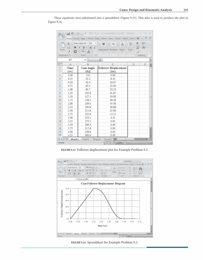
Cams: Design and Kinematic Analysis 235
These equations were substituted into a spreadsheet (Figure 9.15). This data is used to produce the plot in
Figure 9.16.
FIGURE 9.15 Follower displacement plot for Example Problem 9.2.
FIGURE 9.16 Spreadsheet for Example Problem 9.2.

236 CHAPTER NINE
25
Follo
wer
dis
plac
emen
t (m
m)
1 2 3 4
Time (s)
3 = 63.7�
2 = 169.3�β
ββ( 2)/6 = 11.55�
1 = 127�β
50 ...........................................................................................................................................................
......
......
......
......
......
....
......
......
......
......
......
......
....
......
......
......
......
......
......
....
......
......
......
......
......
......
....
......
......
......
......
......
......
....
......
......
......
......
......
......
....
FIGURE 9.17 Follower displacement plot for Example Problem 9.3.
9.5.5 Combined Motion Schemes
In selecting a particular motion scheme, one goal is tominimize the dynamic forces induced during the rise or fallinterval. This is done by minimizing the magnitude ofthe follower acceleration and keeping it continuous.Additionally, the kinetic energy stored in the follower isproportional to the square of the velocity. Thus, minimizingthe maximum velocity is another goal that should be consid-ered when specifying a motion scheme.
In addition to these goals, for high-speed applications itis wise to keep the acceleration smooth to avoid abruptchanges in dynamic loads. The time derivative of the acceler-ation is referred to as jerk. Sudden changes in accelerationare quantified by high magnitudes of jerk. Thus, reducingthe magnitude and maintaining a continuous jerk versustime curve has advantages on machine loading.
Negative aspects of the constant velocity, constant accel-eration, harmonic and cycloidal schemes are often adjustedto improve motion characteristics. The resulting motion iscalled a combined scheme. Descriptions of some of the morecommon combined schemes are given below. More compre-hensive cam design sources should be consulted to obtainthe details of the motion equations [Refs. 5, 11, 14].Software, such as Dynacam, Analytix/Cams, and CamTrax,are available to construct motion follower displacement dia-grams of these and other schemes.
Trapezoidal Acceleration is a scheme that improves onthe constant acceleration scheme shown in Figure 9.10,
where the acceleration versus time curve appears as a squarewave. The difficulty with the square wave is that theacceleration, and consequently inertial force, changesabruptly. Thus, a jerk is induced onto the machine. Thetrapezoidal acceleration scheme softens the transitionswhere the acceleration versus time curve appears as atrapezoid. However, the area lost by knocking off the cornersmust be replaced by increasing the maximum acceleration.
Modified Trapezoidal Acceleration improves on thetrapezoidal scheme by replacing the sloped sides on theacceleration versus time curve with portions of a sine wave.By eliminating the corners, a smooth acceleration curve iscreated. The continuous slope (jerk) ensures that the changein dynamic forces is smooth.
3-4-5 Polynomial Displacement is another scheme thatimproves on the constant acceleration scheme. Being secondorder polynomial, the constant acceleration scheme is hinderedwith a discontinuous acceleration curve. As with the trapezoidalscheme, another method of eliminating the discontinuity is touse a higher-order polynomial. Thus, a scheme has beenformulated that incorporates third, fourth, and fifth orderterms. Having fifth order term, this scheme providescontinuous slope on the acceleration versus time curve.However, the jerk versus time curve will have discontinuities.
4-5-6-7 Polynomial Displacement expands the 3-4-5polyno-mial scheme and includes a seventh order term toprovide a continuous and smooth jerk.
EXAMPLE PROBLEM 9.3
For the application presented in Example Problem 9.2, graphically construct a follower displacement diagram.
SOLUTION: Using the data from Example Problem 9.2, the displacement diagram shown in Figure 9.17 can be constructed. Note
that the circle used to construct the cycloidal fall has a radius of
r =H1
2p=
(50 mm)
2p= 7.96mm

Cams: Design and Kinematic Analysis 237
Modified Sinusoidal Acceleration improves on thecycloidal scheme by incorporating a second sinusoidal termwith a different frequency. Smoothness of the cycloidalmotion is retained and the maximum is reduced.
A summary of the peak velocity, peak acceleration, andpeak jerk for the different motion schemes, as a function ofthe rise H and period of the interval T, is shown in Table 9.5.
the application. In general, a large base circle causes fewerproblems with force transmission. However, a large basecircle and, hence, a large cam is contradictory to thecommon design goal of smaller products.
The trace point serves as a reference to determine theeffective location of the follower. For a knife-edge follower, itis the point of cam and follower contact. For a rollerfollower, the trace point is chosen at the center of the roller.For a flat- or spherical-face follower, the trace point ischosen on the contact surface of the follower.
The home position of the cam is the orientation thatcorresponds to the 0° reference position on adisplacement diagram.
The prime circle is a circle drawn through the trace pointof the follower while the cam is at its home position.
The pitch curve is the path of the center of the follower.
For ease in cam profile construction, kinematic inver-sion will be used. The cam will be imagined as beingstationary. The follower then should be rotated oppositeto the direction of cam rotation. The desired location forthe follower, at several positions, is constructed from the basecircle. Conceptually, this is comparable to wrapping thedisplacement diagram around the base circle, creating thecam shape.
The specific procedures for different follower arrange-ments are illustrated in the following sections. The generaldisplacement diagram shown in Figure 9.19 is used for allconstructions. Notice that follower displacements have beenidentified at specific cam angles from the rise and fallportions of the diagram. These prescribed displacements aretranslated to the cam profile.
9.6.1 In-Line Knife-Edge Follower
The most efficient manner to describe the construction of acam with a knife-edge follower is through an actualconstruction. Using the displacement diagram from Figure9.19, a cam profile to be used with a knife-edge follower hasbeen constructed and shown in Figure 9.20.
The following general procedure is used to graphicallyconstruct such a profile:
1. Draw the base circle of radius Rb. The size is typically afunction of the spatial constraints of the application.
2. Draw the follower in the home position.
3. Draw radial lines from the center of the cam,corresponding to the cam angles identified on thedisplacement diagram. For construction purposes,the cam will remain stationary and the follower will be rotated in a direction opposite to the actual camrotation.
4. Transfer the displacements from the displacement diagram to the radial lines. Measure these displace-ments from the base circle.
5. Draw a smooth curve through these prescribed displacements.
TABLE 9.5 Motion Scheme Comparisons
Motion SchemePeak Velocity
Peak Acceleration Peak Jerk
Constant Velocity 1.000 H/T q qConstant Acceleration 2.000 H/T 4.000 H/T2 qHarmonic 1.571 H/T 4.945 H/T2 qCycloidal 2.000 H/T 6.283 H/T2 40 H/T3
Trapezoidal 2.000 H/T 5.300 H/T2 44 H/T3
Modified Trapezoidal 2.000 H/T 4.888 H/T2 61 H/T3
3-4-5 Polynomial 1.875 H/T 5.777 H/T2 60 H/T3
4-5-6-7 Polynomial 2.188 H/T 7.526 H/T2 52 H/T3
Modified Sine 1.760 H/T 5.528 H/T2 69 H/T3
Trace point, F
Roller follower circle
Home
Offset, e
Rb
RfBase circle
Prime circle
Cam profile
Pitch curve
FIGURE 9.18 Cam nomenclature.
9.6 GRAPHICAL DISK CAM PROFILEDESIGN
Once the desired motion of a cam and follower has beendefined through a displacement diagram, the actual shape ofthe cam can be designed. The shape of the cam depends onthe size of the cam along with the configuration of thefollower. Prior to designing the profile of a disk cam, somegeometric features must be defined. The following featuresare illustrated in Figure 9.18.
The base circle is the smallest circle centered on the camrotation axis and tangent to the cam surface. The size of thebase circle is typically dictated by the spatial restrictions of

238 CHAPTER NINE
6. To accurately construct a profile consistent with thedisplacement diagram, it may be necessary to transferadditional intermediate points from the rise and fallintervals.
9.6.2 In-Line Roller Follower
Again, the most efficient manner of describing theconstruction of a cam with an in-line roller follower isthrough an actual construction. Using the displacementdiagram from Figure 9.19, a cam profile to be used with anin-line roller follower has been constructed and shown inFigure 9.21. The following general procedure is used toconstruct such a profile:
1. Draw the base circle of radius Rb. The size is typically afunction of the spatial constraints of the application.
2. Draw the follower of radius Rf in the home position,tangent to the base circle.
3. Draw radial lines from the center of the cam, correspond-ing to the cam angles identified on the displacement
Trace point
180�
R60
R30
camωR330
R300
R270
R240
R210R180
R150
R120
R90
210�
240�
270�
300�
330�30�
0� (Home)
60�
90�
120�
150� Base circle Cam profile
Δ
ΔΔ
Δ
Δ
Δ
Δ
Δ Δ
Δ
Δ
FIGURE 9.20 Cam profile design—in-line, knife-edge follower.
Follo
wer
dis
plac
emen
tCam angle (deg)
90 180 270 360
ΔR90 ΔR240
.. ......
......
..
......
......
......
......
..
......
......
......
......
......
......
......
......
......
......
......
......
......
......
......
......
......
......
......
....
......
......
......
..
......
...
.
ΔR180
FIGURE 9.19 General follower displacement diagram.
diagram. For construction purposes, the cam will remainstationary and the follower will be rotated in a directionopposite to the actual cam rotation.
4. Identify the trace point at the home position. For aroller follower, this is the point at the center of theroller.
5. Draw the prime circle through the trace point at itshome position.
6. Transfer the displacements from the displacementdiagram to the radial lines. Measure these displace-ments from the prime circle.
7. Draw the roller outline of radius Rf, centered at theprescribed displacements identified in the previous step.
8. Draw a smooth curve tangent to the roller at theseprescribed displacements.
9. To accurately construct a profile consistent with thedisplacement diagram, it may be necessary to transferadditional intermediate points from the rise and fallintervals.

Cams: Design and Kinematic Analysis 239
9.6.3 Offset Roller Follower
The most efficient manner of describing the construction ofa cam with an offset roller follower is through an actualconstruction. Using the displacement diagram from Figure9.19, a cam profile to be used with an offset roller followerhas been constructed and shown in Figure 9.22. The follow-ing general procedure is used to construct such a profile.
1. Draw the base circle of radius Rb. The size is typically afunction of the spatial constraints of the application.
2. Draw the follower centerline in the home position.
3. Draw the prime circle, whose radius is equal to the sumof the base and roller follower radii
4. Draw the follower in the home position of radius Rf,centered where the follower centerline intersects theprime circle.
(Rb 6 Rf).
5. Identify the trace point at the home position. For aroller follower, this is the point that is at the center ofthe roller.
6. Draw an offset circle of radius e, centered at the camrotation axis. It will be tangent to the followercenterline.
7. Draw lines tangent to the offset circle, corresponding tothe reference cam angles on the displacement diagram.For construction purposes, the cam will remainstationary and the follower will be rotated in a direc-tion opposite to the actual cam rotation.
8. Transfer the displacements from the displacementdiagram to the offset lines. Measure these displace-ments from the prime circle.
9. Draw the roller outline of radius Rf, centered at theprescribed displacements identified in the previous step.
+
+
+
+
+
+
+
+
+
+
+
R180
R150
R120
R90
R60
R30
Trace point
180�
camω
210�
240�
270�
300�
330�30�
0� (Home)
60�
90�
120�
150�
Base circle
Prime circle
Cam profile
Pitch curve
ΔR330
ΔR300
ΔR270
ΔR240
ΔR210
FIGURE 9.21 Cam profile design—in-line roller follower.

240 CHAPTER NINE
10. Draw a smooth curve tangent to the roller at theseprescribed displacements.
11. To accurately construct a profile consistent with thedisplacement diagram, it may be necessary to transferadditional intermediate points from the rise and fallintervals.
9.6.4 Translating Flat-Faced Follower
The most efficient manner for describing the construction ofa cam with a flat-faced follower is through an actualconstruction. Using the displacement diagram from Figure9.19, a cam profile to be used with a translating flat-facedfollower has been constructed and shown in Figure 9.23.
The following general procedure is used to graphicallyconstruct such a profile.
1. Draw the base circle of radius Rb. The size is typically afunction of the spatial constraints of the application.
Recall that for this type of follower, the base circle alsoserves as the prime circle.
2. Draw the follower in the home position, tangent to thebase circle.
3. Draw radial lines from the center of the cam, corre-sponding to the cam angles on the displacementdiagram. For construction purposes, the cam willremain stationary and the follower will be rotated ina direction opposite to the actual cam rotation.
4. Transfer the displacements from the displacement dia-gram to the radial lines, measured from the base circle.
5. Draw the flat-faced outline by constructing a line perpen-dicular to the radial lines at the prescribed displacements.
6. Draw a smooth curve tangent to the flat-faced outlines.
7. To accurately construct a profile consistent with the dis-placement diagram, it may be necessary to transfer addi-tional intermediate points from the rise and fall motions.
+
+
+
++
+
+
+
+
+
+
Trace point
180�210�
240�
270�
300�
330�
30�
0� (Home)e
60�
cam
90�
120�
150�
Base circle
Prime circle
Cam profile
Pitch curveOffsetcircle
ΔR330
ΔR300
ΔR270
ΔR240
ΔR210
ΔR150
ΔR120
ΔR90
ΔR60
ΔR30
ΔR180
ω
FIGURE 9.22 Cam profile design—offset roller follower.

Cams: Design and Kinematic Analysis 241
180�
camω
210�
240�
270�
300�
330�30�
0� (Home)
60�
90�
120�
150�Base circle
Cam profile
R330
R300
R270
R240
R210
R180
R150
R120
R90
R60
R30
FIGURE 9.23 Cam profile design—flat-faced follower.
9.6.5 Pivoted Roller Follower
The pivoted follower provides rotational motion as the outputof the cam and follower system. With translating followers,the equations presented in Section 9.5 are used to calculate themagnitude of the instantaneous linear displacement, ΔRF,velocity, vF, and acceleration, aF, of the follower center,point F. For the pivoted follower, the equations presented inSection 9.5 can be used to calculate the instantaneousrotational displacement, ΔθL, velocity, ωL, and acceleration,αL, of the follower link. To use the equations in Section 9.5for rotational motion analysis, the prescribed followerdisplacement must be angular, ΔθL, instead of linear, H.
Again, the most efficient manner of describing the con-struction of a cam with a pivoted roller follower is through anactual construction. Using the displacement diagram fromFigure 9.19, a cam profile to be used with a pivoted rollerfollower has been constructed and shown in Figure 9.24.
The following general procedure is used to graphicallyconstruct such a profile.
1. Draw the base circle of radius Rb, where the size is afunction of the spatial constraints of the application.
2. Draw the prime circle, whose radius is equal to the sumof the base and roller follower radii.
3. Draw the pivot circle of radius Rp. The distance between the pivot and the cam axis is also a function of the spatial constraints of the application.
4. Locate the home position of the pivot.
5. Draw an arc, centered at the home pivot, with a radiusequal to the length of the pivoted follower link, RL.
6. Draw the follower in the home position of radius Rf,centered where the arc drawn in step 5 intersects theprime circle.
7. Draw radial lines from the center of the cam to thepivot circle, corresponding to the cam angles onthe displacement diagram. Recall that the follower isbeing rotated in a direction opposite to the camrotation.

242 CHAPTER NINE
+
+
+
++
+
+
+
++
+
Trace point
Pivot circle
180�
RL
210�
240�
270�
300�
330�30�
0� (Home)
60�
90�
120�
150�
Base circle
Prime circle
Cam profile
Pitch curve
camω
ΔR30
ΔR90
ΔR60
ΔR180
ΔR240 ΔR210
ΔR270
ΔR300
ΔR330
ΔR150
ΔR120
FIGURE 9.24 Cam profile design—pivoted roller follower.
8. From each pivot point, draw an arc with a radius equalto the length of the follower arm, RL, outward from theprime circle.
9. Transfer the displacements from the displacementdiagram to the pivot arcs drawn in step 8. As men-tioned, the prescribed displacements for a pivotedfollower can be angular. Equation (9.3) can be usedto convert from angular displacement of thefollower link, ΔθL, to linear displacement of theroller center, ΔRF.
. (9.3)
10. Draw the roller outline, centered at the prescribeddisplacements identified in the previous step.
11. Draw a smooth curve tangent to the roller at theseprescribed displacements.
12. To accurately construct a profile consistent with the dis-placement diagram, it may be necessary to transfer addi-tional intermediate points from the rise and fall motions.
9.7 PRESSURE ANGLE
Because a force is always transmitted perpendicular tosurfaces in contact, the cam does not always push the followerin the direction of its motion. As discussed in the previoussection, the curvature of the cam affects the position betweenthe follower centerline and the actual contact point.
¢RF = RL32(1 - cos ¢uL)
The force required to push the follower depends on theapplication of the cam system. However, the contact force be-tween the cam and follower can be much greater, dependingon the location of the contact point. Actually, only one compo-nent of the contact force generates the follower motion. Theother force component is undesirable as it generates a side loadand must be absorbed by the follower guide bearings.
The pressure angle, δ, correlates these two componentsof the contact force. The pressure angle, at any point on theprofile of a cam, is the angle between the follower movementand direction that the cam is pushing it. More precisely, it isthe angle between the path of the follower motion and theline perpendicular to the cam profile at the point of followercontact. Each point on the cam surface has a pressure angle.The pressure angle is illustrated in Figure 9.25.
After graphically constructing a cam profile, themagnitude of the pressure angle can be visualized byobserving the location of the contact point in relation tothe follower centerline. The regions where the cam profileexhibits the greatest curvature should be identified.Measurements of the pressure angles in this region shouldbe obtained. In general, the pressure angle should be keptas small as possible and should not exceed 30°. The magni-tude of the pressure angle can be decreased by
1. Increasing the size of the base circle,
2. Decreasing the magnitude of follower displacement,
3. Increasing the angle of cam rotation prescribed for thefollower rise or fall,

Cams: Design and Kinematic Analysis 243
cam, the construction angle increments were refined for in-creased accuracy. The cam profile was constructed bylocating the follower circles and drawing the cam profiletangent to the follower circles. Notice that the cam does notcontact the follower at all locations. At a cam angle of 135°,the cam will not push the roller to the desired position.
This situation can be corrected by using a larger basecircle or reducing the diameter of the roller follower.However, the contact stresses in the cam and follower areincreased if the roller diameter is reduced. Thus, a roller ofexcessively small diameter should be avoided.
A similar situation can occur with a flat-faced follower.Figure 9.27a illustrates a cam segment whose follower alsorequires a rapid rise. Notice that once the flat-facedfollower positions are located, a smooth curve cannot beconstructed to represent the cam profile. One followerconstruction line (90°) falls outside the intersection of theadjacent follower construction lines. Thus, at a cam angleof 90°, the cam will not push the flat-faced follower to itsdesired position.
Figure 9.27b illustrates another cam segment, with alarger base circle. This cam has the exact same displacementrequirements as the one in Figure 9.27a. In this case, asmooth cam profile can be constructed tangent to allfollower construction lines. Again, a functional design wasachieved by increasing the diameter of the base circle.
9.9 ANALYTICAL DISK CAM PROFILEDESIGN
The previous sections illustrated graphical methods usedto design a cam profile. Depending on the precisionrequired for the application, these methods can producesufficiently accurate profiles. Of course, the accuracy isincreased when the construction is accomplished on aCAD system. With CAD, splines are typically used toconstruct the smooth curve of the cam profile. Often,
Unobtainable displacement
0� (Home)
90�
180�
270�
FIGURE 9.26 Impractical cam with a roller follower.
Direction offollower motion
Pressureangle,δ
Contact force
FIGURE 9.25 Pressure angle.
4. Decreasing the amount of follower offset, or
5. Modifying the follower motion scheme.
9.8 DESIGN LIMITATIONS
As seen in Section 9.6, the design of a cam profile cannotbegin until first deciding on a follower type and the locationand size of a base circle. These decisions are usually depen-dent on the magnitude of the transmitted forces and the sizerequirements of the cam-driven machinery. It must beunderstood that these decisions may not always be practical.
Figure 9.26 illustrates a cam with an in-line rollerfollower. Notice that there is a rapid rise and fall at a camangle of 135°. Also note that during this portion of the

244 CHAPTER NINE
splines have precision errors that may violate tangencyconstraints. To increase the accuracy, smaller cam angleincrements can be employed.
In some situations, highly accurate cams are required.It is desirable to be able to analytically determine thecoordinates of points on the cam surface as well as coordi-nates of a milling cutter that will be used to manufacturethe cam. Equations have been developed for thecoordinates of the different types of followers. This sectionmerely presents these equations, and the reader is referredto more detailed sources for the derivations [Ref. 4].Incorporating the equations into a spreadsheet or someother programmable device can quickly generate theprofile coordinates.
In general, a Cartesian coordinate system is used sothat the origin is at the cam center. The positive y-axis isalong the direction of the follower motion in its homeposition. The positive x-axis is 90° clockwise from the y-axis, consistent with a right-hand coordinate system.Figure 9.28 illustrates this coordinate system.
9.9.1 Knife-Edge Follower
The x and y coordinates of the cam profile are given as
(9.3)
(9.4)
where the following notation is used:Rx = x coordinate of cam surface profileRy = y coordinate of cam surface profileRb = Base circle radius
= Cam rotation angle measured against the direction ofcam rotation from the home position
ΔR = Follower displacement at cam angle
Most cams are produced through a cutting operation,using computer numerical control milling machines. Thesemachines are capable of rotating the cam by a fraction of adegree, while advancing the cutter by thousandths of amillimeter. Through this method, the cam profile can beprecisely manufactured.
f
f
Ry = (Rb + ¢R)cosf
Rx = (Rb + ¢R) sinf
Cam profilecoordinatesRx and Ryat cam angle
y
Followeroffset, e
Cam angle,
φφ
ω
φ
x
Base circleradius, Rb
Home ( = 0�)φ
Rollerfollowerradius, Rf
FIGURE 9.28 Cam profile coordinate system.
90�
90�
120�
120�
150�
150�
180�180�
(a) (b)
60�
Unobtainable displacement 60�
30�
30�
0� (Home) 0� (Home)
FIGURE 9.27 Impractical cam with a flat-faced follower.

Cams: Design and Kinematic Analysis 245
FIGURE 9.29 Coordinates for Example Problem 9.4.
The x and y coordinates of the center of the millingcutter, or grinding wheel, are given as
(9.6)
(9.7)Cy = (Rc + Rb + ¢R)cosf
Cx = (Rc + Rb + ¢R) sinf
where the following additional notation is used:Cx = x coordinate of cutter centerCy = y coordinate of cutter centerRc = Mill cutter radius
EXAMPLE PROBLEM 9.4
For the application stated in Example Problem 9.2, analytically determine the cam profile coordinates when a knife-
edge follower is incorporated. Because of the size constraints of the machine, a cam with a base circle diameter of
200 mm must be used. The cam is to rotate counterclockwise.
SOLUTION: 1. Calculate Coordinates of the Cam Profile
The base circle radius is half of the base circle diameter; thus
Substitution into equations (9.4) and (9.5) gives
2. Summarize the Profile Coordinates for Several Cam Angles
Inserting these equations into a spreadsheet gives the results listed in Figure 9.29.
3. Plot the Profile Coordinates
A spreadsheet can be used to easily create a plot of the profile coordinates. This plot is shown as Figure 9.30 and
illustrates the cam profile.
Ry = (Rb + ¢R)cosf = [(100mm) + ¢R]cosf
Rx = (Rb + ¢R) sinf = [(100 mm) + ¢R] sinf
Rb = 100mm
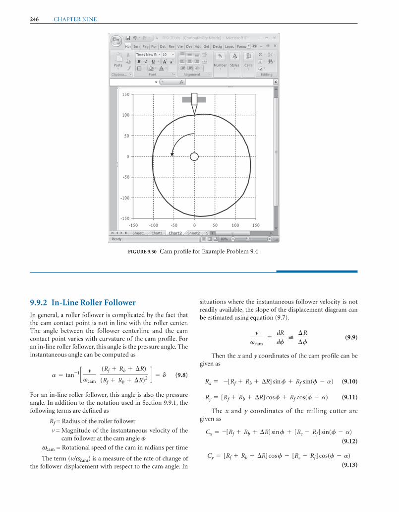
246 CHAPTER NINE
FIGURE 9.30 Cam profile for Example Problem 9.4.
9.9.2 In-Line Roller Follower
In general, a roller follower is complicated by the fact thatthe cam contact point is not in line with the roller center.The angle between the follower centerline and the camcontact point varies with curvature of the cam profile. Foran in-line roller follower, this angle is the pressure angle. Theinstantaneous angle can be computed as
(9.8)
For an in-line roller follower, this angle is also the pressureangle. In addition to the notation used in Section 9.9.1, thefollowing terms are defined as
Rf = Radius of the roller follower
v = Magnitude of the instantaneous velocity of thecam follower at the cam angle
ωcam = Rotational speed of the cam in radians per time
The term (v/ωcam) is a measure of the rate of change ofthe follower displacement with respect to the cam angle. In
f
a = tan-1 c v
vcam
(Rf + Rb + ¢R)
(Rf + Rb + ¢R)2 d = d
situations where the instantaneous follower velocity is notreadily available, the slope of the displacement diagram canbe estimated using equation (9.7).
(9.9)
Then the x and y coordinates of the cam profile can begiven as
(9.10)
(9.11)
The x and y coordinates of the milling cutter aregiven as
(9.12)
(9.13)
Cy = [Rf + Rb + ¢R]cosf - [Rc - Rf]cos(f - a)
Cx = -[Rf + Rb + ¢R] sinf + [Rc - Rf] sin(f - a)
Ry = [Rf + Rb + ¢R]cosf + Rf cos(f - a)
Rx = -[Rf + Rb + ¢R] sinf + Rf sin(f - a)
v
vcam=
dR
df�
¢R
¢f

Cams: Design and Kinematic Analysis 247
SOLUTION: 1. Calculate the Time for a Full Cycle
The total time to complete the full cycle is needed to determine the required speed of the cam.
2. Calculate the Required Rotational Speed of the Cam
From equation (9.2),
3. Determine the Cam Rotation for Each Follower Motion Interval
The angular increment of the cam consumed by each follower motion sequence is determined by equation (9.1).
4. Calculate the Displacements during Each Follower Motion Interval
The equations for the harmonic rise and fall were given in Table 9.3. Substituting into the harmonic rise
equations gives
¢R1 =H1
2c1 - cosapt1
T1b d =
(1.5 in.)
2c1 - cosa pt1
1.5 sb d
b4 = 10.143rev/s2 (2.0 s) = 0.286rev = 102.8°
b3 = 10.143rev/s2 (1.5 s) = 0.214rev = 77.2°
b2 = 10.143rev/s2 (2.0 s) = 0.286rev = 102.8°
b1 = (vcam)(T1) = 10.143rev/s2 (1.5 s) = 0.214rev = 77.2°
vcam =1rev
©Ti=
1rev
7s= 0.143rev/s = 0.899rad/s = 8.57rpm
= 1.5 + 2.0 + 1.5 + 2.0 = 7.0 s
©Ti = T1 + T2 + T3 + T4
EXAMPLE PROBLEM 9.5
Two cams are used to drive a gripper of a mechanical part handler. The two cams can generate independent horizon-
tal and vertical motions to the gripper. Such machines can relocate parts in a similar fashion to a robot at a fraction of
the cost. The part handler is shown in Figure 9.31.
The prescribed motion for one of the cam followers is as follows:
1. Rise 1.5 in. in 1.5 s using the harmonic motion scheme.
2. Dwell for 2 s.
3. Return in 1.5 s using the harmonic motion scheme.
4. Dwell for 2 s.
5. Repeat the sequence.
An in-line roller follower with a radius of 0.5 in. is used on a cam with a base circle radius of 3.5 in. Tabulate the
follower motion and specify the coordinates of the cam profile.
FIGURE 9.31 Part-handling machine for Example Problem 9.5.

248 CHAPTER NINE
Substituting into the harmonic fall equations gives
5. Calculate the Coordinates of the Cam Profile
Substitution into equations (9.8), (9.10), and (9.11) gives
6. Summarize the Profile Coordinates for Several Cam Angles
Inserting these equations into a spreadsheet gives the results listed in Figure 9.32.
7. Plot the Profile Coordinates
A spreadsheet can be used to easily create a plot of the profile coordinates. This plot is shown as Figure 9.33 and
illustrates the cam profile.
Ry = -[Rf + Rb + ¢R]cosf + Rf cos(f - a) = -[0.5 + 3.5 + ¢R]cosf - 0.5cos(f - a)
Rx = -[Rf + Rb + ¢R] sinf + Rf sin(f - a) = -[0.5 + 3.5 + ¢R] sinf + 0.5sin(f - a)
a = tan-1 c v
vcam
[Rf + Rb + s]
[Rf + Rb + s]2 d = tan-1 c v
10.899rad/s2[(0.5 in.) + (3.5 in.) + s]
[(0.5 in.) + (3.5 in.) + s]2 d
v2 =- pH2
2T2csin apt2
T2b d =
- p(1.5 in.)
2(1.5 s)csin a pt2
1.5 sb d
¢R2 =H2
2c1 + cosapt2
T2b d =
(1.5 in.)
2c1 + cosa pt2
1.5 sb d
v1 =pH1
2T1csin apt1
T1b d =
p11.5 in.2211.5s2 csin a pt1
1.5 sb d
FIGURE 9.32 Cam profile coordinates for Example Problem 9.5.

Cams: Design and Kinematic Analysis 249
9.9.3 Offset Roller Follower
An offset roller follower is further complicated by the factthat the follower motion is not in line with the cam contactpoint, which, in turn, is not in line with the roller center.Thus, the profile equations become a bit more complex. Theangle between the lines connecting the follower center withthe cam contact point, and the follower center with the camcenter is computed as
(9.14)
As in equation (9.8), the term (v/ωcam) is a measure of therate of change of the follower displacement with respect tothe cam angle. In situations where the instantaneousfollower velocity is not readily available, the slope of thedisplacement diagram can be estimated using equation(9.9). The pressure angle, δ, can be calculated as
(9.15)
As before, the offset distance, e, is defined as the distancebetween the follower centerline and the cam center. A posi-tive offset distance is defined in the positive x direction.Conversely, a negative offset distance is defined in the
d = a - tan-1a e
Rf + Rb + ¢Rb
a Rf + Rb + ¢R
e2 + (Rf + Rb + ¢R)2 - e 1n/vcam2bd
a = tan-1 c a nvcam
b
negative x direction. The offset distance shown in Figure9.28 is a positive value. Then the x and y coordinates of thecam profile can be given as
(9.16)
(9.17)
The x and y coordinates of the milling cutter are given as
(9.18)
(9.19)
9.9.4 Translating Flat-Faced Follower
The analytical construction of a translating flat-facedfollower can also exhibit a contact point that is not in linewith the cam centerline. The angle between the followercenterline and the line connecting the cam contact pointwith the cam center varies with the curvature of the camprofile and can be computed as
(9.20)a = tan-1e a v
vcamb 1
(Rb + ¢R)f
- [Rc - Rf ] cos (f - a)
Cy = (e)sinf - [Rf + Rb + ¢R] cos f
+ [Rc - Rf] sin(f - a)
Cx = (e)cosf - [Rf + Rb + ¢R] sin f
Ry = (e)sin f - [Rf + Rb + ¢R] cos f + Rf cos (f - a)
Rx = (e)cosf - [Rf + Rb + ¢R] sinf + Rf sin(f - a)
FIGURE 9.33 Cam profile for Example Problem 9.5.

As in equations (9.8) and (9.14), the term (v/ωcam) is a mea-sure of the rate of change of the follower displacement withrespect to the cam angle. In situations where the instantaneousfollower velocity is not readily available, the slope of the dis-placement diagram can be estimated using equation (9.9).
Then the x and y coordinates of the cam profile can begiven as
(9.21)
(9.22)
The x and y coordinates of the milling cutter are given as
(9.23)
(9.24)
where
(9.25)
9.9.5 Pivoted Roller Follower
The analytical construction of a pivoted roller followeris similar to the offset translating follower. However, thegeometry and definitions are slightly different. Figure 9.34illustrates the nomenclature used for a cam with a pivotedroller follower.
g = tan-1 c (Rb + ¢R)tan(a)
Rc + Rb + ¢Rd
Cy = c Rb + ¢R + Rc
cosgd sin(f + g)
Cx = c Rb + ¢R + Rc
cosgd cos(f + g)
Ry = aRb + ¢R
cosab sin(f + a)
Rx = aRb + ¢R
cosab cos(f + a)
250 CHAPTER NINE
Cam profilecoordinatesRx and Ryat cam angle
Home ( = 0�)φy
RL
Rp
Rf
ΔθL
Δ R
x
φ
φ
Rb
F
FIGURE 9.34 Cam profile coordinate system, with a pivoted follower.
The following notation is used:
RL = Length of the follower pivot link
RP = Distance between the cam center and the pivotlocation
ΔθL = Instantaneous angular position of the followerpivot link
ωL = Instantaneous angular velocity of the followerpivot link
αL = Instantaneous angular acceleration of the fol-lower pivot link
The main difference with a pivoted follower is that itsmotion is rotational and the prescribed motion is usually theangular position of the follower versus time, or cam angle.Equation (9.3) gave the relation between the angular dis-placement of the follower link and the linear displacement ofthe roller center, point F.
(9.3)
The velocity of the follower center can be related to the rota-tional velocity of the follower link.
(9.26)
Again, the angle between the lines connecting thefollower center with the cam contact point and the followercenter with the cam center varies with the curvature of thecam profile and can be computed as
(9.27)a 1
(Rf + ¢R + Rb) - 1v/vcam2cosgb d
aL = tan-1 c a v
vcamb
vF = RLvL
¢RF = RL32(1 - cos ¢uL)

Cams: Design and Kinematic Analysis 251
9.10.1 Graphical Cylindrical Cam Profile Design
The most efficient manner for describing the construction of acylindrical cam is through an actual construction. Using thedisplacement diagram from Figure 9.19, a cylindrical camprofile has been constructed and shown in Figure 9.35. Thefollowing general procedure is used to construct such a profile:
1. Draw a straight line equal to the circumference of thecylindrical cam.
2. Divide this line into sections corresponding to thereference cam angles on the displacement diagram.
3. Transfer the displacements from the displacementdiagram to the lines corresponding to the referencecam angles.
4. Draw the roller follower at the prescribed displacements.
5. Draw a smooth curve tangent to the roller outlines.
6. To accurately construct a profile consistent with the dis-placement diagram, it may be necessary to transfer addi-tional intermediate points from the rise and fall motions.
0
Z
90 180 270 360
ΔR90ΔR240
FIGURE 9.35 Cylindrical cam profile design.
As before, the term (vF/ωcam) is a measure of the rate ofchange of the follower displacement with respect to the camangle. In situations where the instantaneous follower veloc-ity is not readily available, the slope of the displacementdiagram can be estimated using equation (9.9).
Internal angles are given as
(9.28)
(9.29)
(9.30)
Finally, the x and y coordinates of the cam profile can be givenas
(9.31)
(9.32)
and the pressure angle is given as
(9.33)
The x and y coordinates of the milling cutter are given as
(9.34)
(9.35)
9.10 CYLINDRICAL CAMS
Although disk cams are the most common type of cam, cylin-drical cams are also widely used. As presented in Section 9.2and illustrated in Figure 9.3b, a cylindrical cam consists of agroove wrapped around a cylinder. A cylindrical cam is a posi-tive motion cam in that the follower is constrained in a grooveand an external member is not needed to maintain contact be-tween the follower and the cam. There are many applicationsin which it is necessary for the cam to exert a positive control ofthe follower during the rise or fall sequences.
Often, a tapered roller follower is used as shown inFigure 9.3b. It is used because the top edge of the groovetravels at a higher speed than the bottom portion. Thus, thetaper can compensate for the speed differential and preventany slipping and skidding action of the roller. When acylindrical roller is used, it is advisable to use a narrowwidth to minimize the velocity difference across the face ofthe roller.
In general, calculation and layout procedures are similarto those for the disk cam. The following sections discussprofile generation techniques for a cylindrical cam with atranslating follower. The profile generation for other types offollowers are similar.
Cy = [Rf + Rb + ¢R] sinb - [Rc - Rf]cos(b - a)
Cx = [Rf + Rb + ¢R]cosb - [Rc - Rf] sin(b - a)
d = g + a -p
2
Ry = - [Rf + Rb + ¢R] sinb - Rf cos (b - a)
Rx = - [Rf + Rb + ¢R]cosb - Rf sin(b - a)
b =p
2+ f + a
f = cos-1 c aRp2 + (Rb + Rf + ¢R)2 - RL
2
2(Rp) (Rb + Rb + s)b d
g = cos-1 c aRL2 + (Rb + Rf + ¢R)2 - Rp
2
2(RL) (Rb + Rb + s)b d
9.10.2 Analytical Cylindrical Cam Profile Design
Because a cylindrical cam is wrapped around a cylinder, acylindrical coordinate system is used to define the grooveprofile. The angular coordinate, θ, is the angle around thecam, and the z-axis is the axial position on the cam. Theangle between the follower centerline and the cam contactpoint varies with the curvature of the groove profile and canbe computed as
(9.36)
The notation used is the same as in the precedingsections. For a translating follower, this angle is also thepressure angle. Similar to disk cams, the pressure angleshould be kept to a minimum and not exceed 30°.
The z-coordinate of the upper groove profile, when thefollower center is at , can be given as
(9.37)
(9.38)u = f - tan-1a Rf cosa
Rbb
Rz = ¢R + Rf cosa
f
aL = tan-1a vF
vcamb

252 CHAPTER NINE
Here, Rb is the radius of the cylindrical cam.The z-coordinate of the lower groove profile, when the
follower center is at , can be given as
(9.39)
(9.40)
The coordinate of the milling cutter is given as
(9.41)
(9.42)
9.11 THE GENEVA MECHANISM
A geneva mechanism is a unique design that produces arepeated indexing motion from constant rotational motion.Because of this motion, the geneva mechanism is commonlyclassified with cams. A four-station geneva mechanism isillustrated in Figure 9.36.
The geneva mechanism consists of a driving roller and ageneva wheel. The geneva wheel consists of a disk withseveral radial slots and is fastened to an output shaft. Thedriving roller is fastened to an arm that, in turn, is fastenedto the input shaft. The arm is usually attached to a lockingdisk that prevents the wheel from rotating when the drivingroller is not engaged in a slot. The locking disk fits into acutout on the wheel.
The motion of the geneva mechanism is characterizedby the roller entering a slot in the wheel, indexing the wheel.When the roller exits the slot, the wheel locks into positionuntil the roller enters the next slot. In Figure 9.36a, theroller rotates clockwise and is just about to enter the genevawheel. In Figure 9.36b, the roller has entered the slot andhas turned the wheel counterclockwise. Notice that thelocking disk has moved away from the wheel, allowing it torotate.
When designing a wheel, it is important that the rollerenters the slot tangentially. Otherwise, impact loads arecreated and the mechanism will perform poorly at highspeeds or loads. Because of this constraint, the followinggeometric relationships are derived [Ref. 7]. Refer to Figure9.36 for definitions of the geometric properties.
(9.43)
wheren = Number of stations in the geneva wheel
(9.44)
(9.45)
(9.46)R = d cosa bo
2b
a = d sina bo
2b
go = 90°-bo
2
bo =360°
n
u = f
Cz = ¢R
u = f + tan-1a Rf cosa
Rbb
Rz = ¢R - Rf cosa
f
(9.47)
The kinematics of the geneva wheel can also be analyticallydetermined. The angle of the roller, Δγ, is defined from the startof engagement. The angle of the wheel, measured from thestart of engagement, is defined as β and is calculated as
(9.48)
where
(9.49)
(9.50)
whereΔγ = Amount of rotation of driving from the position wherethe roller has just entered the slot.
The instantaneous velocity and acceleration of thegeneva wheel have been found [Ref. 7] by
(9.51)
(9.52)
These equations are derived using the typical angularsign convention. That is, ω and α are positive when counter-clockwise and negative when clockwise.
+ a arb (vinput shaft)
2 sin(2b - 2c)
(ainput shaft) cos(b - c)- a arb
awheel = - a arb (vinput shaft)
2 sin(b - c)
vwheel = a arb (vinput shaft) cos(b - c)
c = 180° - go + ¢g
r = 3a2 + d2 - 2ad cos(180 - c)
b = sin-1[1 ar2 sin(180° - c)]
S 6 d - a
(b)
(a)
r
Geneva wheel
CrankR
Driving roller
Lockingdisk
Driving roller entersthe geneva slot
d
a
0γ
0γΔγ
0β
β
ω
φ
ω
S
FIGURE 9.36 Four-station geneva mechanism.

Cams: Design and Kinematic Analysis 253
15�
Driving roller entersthe geneva slot
ω
FIGURE 9.37 Geneva mechanism for Example Problem 9.6.
EXAMPLE PROBLEM 9.6
A geneva mechanism has been designed with six stations, as shown in Figure 9.37. The distance between the driving
and driven shafts is 80 mm. The driving arm rotates at a constant rate of 80 rpm clockwise. Determine the angular
velocity and acceleration of the wheel when the driving arm has rotated 15° from the position where the roller has just
entered the slot.
SOLUTION: 1. Calculate Geneva Geometry
Equations (9.43) through (9.47) can be used to calculate the geometric properties of this geneva
mechanism.
2. Calculate Geneva Kinematic Properties
Equations (9.48) through (9.52) can be used to determine the kinematic relationships when the driving arm has
rotated 15° from the position where the roller has just entered the slot.
vinput shaft = 80rpm = -8.4 rad/s, cw
b = sin-1 c a
rsinc d = sin-1 c 40mm
58.94mmsin45° d = 28.7°
= 3(40mm)2 + (80mm)2 - 2(40 mm)(80 mm)cos(45°) = 58.94mm
r = 3a2 + d 2 - 2ad cos(180 - c)
c = 180° - go + ¢g = 180° - 60° + 15° = 135°
¢g = 15°
S 6 d - a = 80 - 40 = 40mm
R = d cos a bo
2b = (80 mm)cos a 60°
2b = 69.3mm
a = d sina bo
2b = (80 mm)sin a 60°
2b = 40mm
go = 90° -bo
2= 90° -
60
2= 60°
bo =360°
n=
360°
6= 60°
254 CHAPTER NINE
PROBLEMS
For graphical solutions, manual techniques can be instructive,but the use of a CAD system is highly recommended.
Graphical Displacement Diagrams
9–1. A cam is required for an automated transfer mech-anism. The cam follower must rise outward 1.0 in.with constant velocity in 3.0 s, dwell for 0.5 s, fallwith constant velocity in 2.0 s, and then repeat thesequence. Determine the required speed of thecam and graphically plot a follower displacementdiagram.
9–2. A cam is required for a reciprocating follower for apick-and-place robotic arm. The cam follower mustrise outward 0.75 in. with constant velocity in 1.4 s,dwell for 2.3 s, fall with constant velocity in 0.8 s,dwell for 1.9 s, and then repeat the sequence.Determine the required speed of the cam andgraphically plot a follower displacement diagram.
9–3. A cam drive is required for a shaker platform. Thisplatform is used to test the shipping-worthiness ofpackaged items. The cam follower must rise outward1.0 in. with constant acceleration in 0.7 s, dwell for0.2 s, fall with constant acceleration in 0.5 s, and thenrepeat the sequence. Determine the required speedof the cam and graphically plot a follower displace-ment diagram.
9–4. A cam drive is required for a mechanism that feedspapers into a printing press. The cam follower mustrise outward 1.0 in. with constant acceleration in 1.7 s,dwell for 0.8 s, fall 0.5 in. with constant acceleration in0.8 s, dwell for 0.3 s, fall 0.5 in. with constant accelera-tion in 0.8 s, and then repeat the sequence. Determinethe required speed of the cam and graphically plot afollower displacement diagram.
9–5. A cam drive is required for an automated slide on ascrew machine that turns intricate parts. The cam
follower must rise outward 1.5 in. with constantacceleration in 1.2 s, dwell for 0.7 s, fall 0.5 in. withconstant acceleration in 0.9 s, dwell for 0.5 s, fall 1.0 in.with constant acceleration in 1.2 s, and then repeat thesequence. Determine the required speed of the camand graphically plot a follower displacement diagram.
9-6. A cam drive is used for a mechanism that drives anautomated assembly machine. The cam followermust rise outward 13 mm with constant velocity in3 s, dwell for 3 s, fall 5 mm with constant accelera-tion in 2 s, dwell for 3 s, fall 8 mm with constantacceleration in 2 s, and then repeat the sequence.Determine the required speed of the cam andgraphically plot a follower displacement diagram.
9–7. A cam drive is used for a mechanism that tests thedurability of oven doors. The cam follower must riseoutward 2 in. with harmonic motion in 1 s, dwell for0.5 s, fall 2 in. with harmonic motion in 1 s, dwell for1 s, and then repeat the sequence. Determine therequired speed of the cam and graphically plot afollower displacement diagram.
9–8. A cam drive is used for a mechanism that moves a toolin an automated screw machining process. The camfollower must rise outward 24 mm with harmonicmotion in 0.2 s, dwell for 0.3 s, fall 10 mm withharmonic motion in 0.3 s, dwell for 0.2 s, fall 14 mmwith harmonic motion in 0.2 s, and then repeat the se-quence. Determine the required speed of the cam andgraphically plot a follower displacement diagram.
9–9. A cam drive is used for a mechanism that packsstuffing into shipping boxes. The cam follower mustrise outward 1 in. with cycloidal motion in 1.5 s, fall1 in. with cycloidal motion in 1 s, dwell for 0.5 s, andthen repeat the sequence. Determine the requiredspeed of the cam and graphically plot a followerdisplacement diagram.
9–10. A cam drive is used for a mechanism incorporatedin a shoe-sewing machine. The cam follower must
= +67.1rad/s2 = +67.1rad/s2, ccw
+ a 40mm
58.94mmb21 -8.4rad/s22sin[2(28.7°) - 2(135°)]
= a 40mm
58.94mmb21 -8.4 rad/s22sin (28.7° - 135°) - 0
+ a a
rb2
(vinput shaft)2sin(2b - 2a)
awheel = - a a
rb (vinput shaft)
2sin(b - a) - a a
rb (ainput shaft) cos(b - a)
ainput shaft = 0(constant angular velocity of input shaft)
vwheel = a a
rb (vinput shaft) cos(b - c) = a 40mm
58.94mmb 1-8.4 rad/s2cos(28.7° - 135°) = + 1.6rad/s = 15.3 rpm, ccw

Cams: Design and Kinematic Analysis 255
rise outward 0.5 in. with cycloidal motion in 0.7 s,dwell for 0.2 s, fall 0.25 in. with cycloidal motion in0.5 s, dwell for 0.2 s, fall 0.25 in. with cycloidalmotion in 0.5 s and then repeat the sequence.Determine the required speed of the cam andgraphically plot a follower displacement diagram.
9–11. A cam drive is required to synchronize two motionson an automated transfer device. The cam followermust rise outward 10 mm with constant accelera-tion in 90° of cam rotation, dwell for 30°, fall 10 mmwith constant acceleration in 180° of cam rotation,and dwell for 60°. Graphically plot a followerdisplacement diagram.
9–12. A cam is used for an exhaust valve in an engine. Thecam follower must rise outward 0.5 in. withharmonic motion in 150° of cam rotation, dwell for30°, and fall 0.5 in. with harmonic motion in 180° ofcam rotation. Graphically plot a follower displace-ment diagram.
9–13. A cam is used for a newspaper-collating device. Thecam follower must rise outward 0.5 in. withcycloidal motion in 120° of cam rotation, dwell for30°, fall 0.5 in. with cycloidal motion in 120° of camrotation, dwell for 30°, and fall 0.5 in. with cycloidalmotion in 60° of cam rotation. Graphically plot afollower displacement diagram.
Analytical Displacement Diagram
For problems 9–14 through 9–23, determine the speed of thecam and use the motion equations and a spreadsheet to plot adisplacement diagram of the follower. Also calculate the max-imum velocity and acceleration of the follower.
9–14. Use the required cam follower motion specified inProblem 9–1.
9–15. Use the required cam follower motion specified inProblem 9–2.
9–16. Use the required cam follower motion specified inProblem 9–3.
9–17. Use the required cam follower motion specified inProblem 9–4.
9–18. Use the required cam follower motion specified inProblem 9–5.
9–19. Use the required cam follower motion specified inProblem 9–6.
9–20. Use the required cam follower motion specified inProblem 9–7.
9–21. Use the required cam follower motion specified inProblem 9–8.
9–22. Use the required cam follower motion specified inProblem 9–9.
9–23. Use the required cam follower motion specified inProblem 9–10.
For problems 9–24 through 9–26, use the motion equa-tions and a spreadsheet to plot a displacement diagram ofthe follower.
9–24. Use the required cam follower motion specified inProblem 9–11.
9–25. Use the required cam follower motion specified inProblem 9–12.
9–26. Use the required cam follower motion specified inProblem 9–13.
Analytical Motion Curves
For problems 9–27 through 9–36, use the motion equationsand a spreadsheet to generate plots of the follower displace-ment, velocity, and acceleration versus time.
9–27. Use the required cam follower motion specified inProblem 9–1.
9–28. Use the required cam follower motion specified inProblem 9–2.
9–29. Use the required cam follower motion specified inProblem 9–3.
9–30. Use the required cam follower motion specified inProblem 9–4.
9–31. Use the required cam follower motion specified inProblem 9–5.
9–32. Use the required cam follower motion specified inProblem 9–6.
9–33. Use the required cam follower motion specified inProblem 9–7.
9–34. Use the required cam follower motion specified inProblem 9–8.
9–35. Use the required cam follower motion specified inProblem 9–9.
9–36. Use the required cam follower motion specified inProblem 9–10.
Graphical Plate Cam Profile Design
9–37. A plate cam must provide the displacement shownin Figure P9.37 to a reciprocating in-line knife-edgefollower. The cam must have a base circle of 3.0 in.and rotate clockwise. Graphically construct theprofile.
9–38. A plate cam must provide the displacement shownin Figure P9.37 to a reciprocating in-line knife-edgeroller follower. The cam must have a base circle of2.0 in. and rotate counterclockwise. Graphicallyconstruct the profile.
9–39. A plate cam must provide the displacement shownin Figure P9.37 to a reciprocating in-line roller fol-lower. The roller diameter is 1.0 in. The cam musthave a base circle of 3.0 in. and rotate clockwise.Graphically construct the profile and estimate thelargest pressure angle.
9–40. A plate cam must provide the displacement shownin Figure P9.37 to a reciprocating in-line rollerfollower. The roller diameter is 0.75 in. The cammust have a base circle of 2.0 in. and rotate counter-clockwise. Graphically construct the profile andestimate the largest pressure angle.

256 CHAPTER NINE
300
Follo
wer
dis
plac
emen
t (in
.)
60
Cam angle (deg)
Cam
angle
0
10
20
30
40
50
60
70
80
90
100
110
120
0.000
0.000
0.000
0.000
0.004
0.029
0.091
0.196
0.337
0.500
0.663
0.804
0.909
(deg)
Follower
Displ.
(in.)
90 120 150 180 210 240 270 300 330 3600.0
0.2
0.4
0.6
0.8
1.0
1.2
Cam
angle
130
140
150
160
170
180
190
200
210
220
230
240
0.971
0.996
1.000
1.000
1.000
1.000
0.996
0.971
0.909
0.804
0.663
0.500
(deg)
Follower
Displ.
(in.)
Cam
angle
250
260
270
280
290
300
310
320
330
340
350
360
0.337
0.196
0.091
0.029
0.004
0.000
0.000
0.000
0.000
0.000
0.000
0.000
(deg)
Follower
Displ.
(in.)
FIGURE P9.37 Problems 37–44 and 47–54.
9–41. A plate cam must provide the displacement shown inFigure P9.37 to a reciprocating offset roller follower.The follower is positioned in the vertical plane, con-tacting the top of the cam. The offset distance is 0.75in. to the left of the cam center. The roller diameter is1.0 in. The cam must have a base circle of 3.0 in. androtate clockwise. Graphically construct the profileand estimate the largest pressure angle.
9–42. A plate cam must provide the displacement shown inFigure P9.37 to a reciprocating offset roller follower.The follower is positioned in the vertical plane, con-tacting the top of the cam. The offset distance is 0.5in. to the right of the cam center. The roller diameteris 0.75 in. The cam must have a base circle of 2.0 in.and rotate counterclockwise. Graphically constructthe profile and estimate the largest pressure angle.
9–43. A plate cam must provide the displacement shownin Figure P9.37 to a reciprocating flat-facedfollower. The cam must have a base circle of 5.0 in.
and rotate clockwise. Graphically construct the pro-file and estimate the largest pressure angle.
9–44. A plate cam must provide the displacement shownin Figure P9.37 to a reciprocating flat-facedfollower. The cam must have a base circle of 6.0 in.and rotate counterclockwise. Graphically con-struct the profile and estimate the largest pressureangle.
9–45. A plate cam must provide the displacement shownin Figure P9.45 to a pivoted roller follower. Thelength of the follower link is 4 in. and is pivoted 5 in.from the cam rotation axis. The roller diameter is 1in. The cam must have a base circle of 3.0 in. androtate clockwise. Graphically construct the profileand estimate the largest pressure angle.
9–46. A plate cam must provide the displacement shownin Figure P9.45 to a pivoted roller follower. Thelength of the follower link is 3 in. and is pivoted3.5 in. from the cam rotation axis. The roller

Cams: Design and Kinematic Analysis 257
300
Follo
wer
dis
plac
emen
t (m
m)
60
Cam angle (deg)
Cam
angle
0
10
20
30
40
50
60
70
80
90
100
110
120
0.000
0.113
0.865
2.725
5.865
10.113
15.000
19.887
24.135
27.275
29.135
29.887
30.000
(deg)
Follower
Displ.
(mm)
90 120 150 180 210 240 270 300 330 3600.0
5.0
10.0
15.0
20.0
25.0
30.0
35.0
Cam
angle
130
140
150
160
170
180
190
200
210
220
230
240
30.000
30.000
30.000
30.000
30.000
30.000
29.966
29.736
29.135
28.035
26.369
24.135
(deg)
Follower
Displ.
(mm)
Cam
angle
250
260
270
280
290
300
310
320
330
340
350
360
21.402
18.300
15.000
11.700
8.598
5.865
3.631
1.965
0.865
0.264
0.034
0.000
(deg)
Follower
Displ.
(mm)
FIGURE P9.45 Problems 45, 46, 55, and 56.
diameter is 0.75 in. The cam must have a basecircle of 2.0 in. and rotate counterclockwise.Graphically construct the profile and estimate thelargest pressure angle.
Analytical Plate Cam Profile Design
For problems 9–47 through 9–56, use the specific cam profileequations and a spreadsheet to generate a chart of profilecoordinates for every 10° of cam angle.
9–47. Use the cam described in Problem 9–37.
9–48. Use the cam described in Problem 9–38.
9–49. Use the cam described in Problem 9–39.
9–50. Use the cam described in Problem 9–40.
9–51. Use the cam described in Problem 9–41.
9–52. Use the cam described in Problem 9–42.
9–53. Use the cam described in Problem 9–43.
9–54. Use the cam described in Problem 9–44.
9–55. Use the cam described in Problem 9–45.
9–56. Use the cam described in Problem 9–46.
Graphical Cylindrical Cam Design
9–57. A cylindrical cam must provide the displacementshown in Figure P9.37 to a reciprocating rollerfollower. The roller diameter is 1.0 in. The cylinderdiameter is 5 in. and rotates clockwise. Graphicallyconstruct the profile and estimate the largestpressure angle.
9–58. A cylindrical cam must provide the displacementshown in Figure P9.37 to a reciprocating rollerfollower. The roller diameter is 30 mm. The cylinderdiameter is 150 mm and rotates clockwise.Graphically construct the profile and estimate thelargest pressure angle.

258 CHAPTER NINE
Analytical Cylindrical Cam Design
For problems 9–59 and 9–60, use the cylindrical cam profileequations and a spreadsheet to generate a chart of profilecoordinates for every 10° of cam angle.
9–59. Use the cam described in Problem 9–57.
9–60. Use the cam described in Problem 9–58.
Geneva Mechanism Problems
9–61. A geneva mechanism has been designed with fourstations. The distance between the driving anddriven shafts is 3 in. The driving arm rotates at a con-stant rate of 60 rpm counterclockwise. Determinethe angular velocity and acceleration of the wheelwhen the driving arm has rotated 25° from the posi-tion where the roller has just entered the slot.
9–62. A geneva mechanism has been designed with fivestations. The distance between the driving anddriven shafts is 60 mm. The driving arm rotates at aconstant rate of 70 rpm clockwise. Determine theangular velocity and acceleration of the wheel whenthe driving arm has rotated 20° from the positionwhere the roller has just entered the slot.
9–63. A geneva mechanism has been designed with six sta-tions. The distance between the driving and drivenshafts is 4 in. The driving arm rotates at a constantrate of 90 rpm counterclockwise. Determine theangular velocity and acceleration of the wheel whenthe driving arm has rotated 25° from the positionwhere the roller has just entered the slot.
CASE STUDIES
9–1. The cam shown in Figure C9.1 is used to feed papersto a printing press. Carefully examine the compo-nents of the mechanism, then answer the followingleading questions to gain insight into its operation.
1. As shaft G is forced to turn clockwise, determine themotion of item E.
2. What is the name of the connection between items Eand F?
3. What causes the stack of papers, sitting on item J, toremain at a level where a mechanism at B can grabthem?
4. Why does the radius on item H change?5. What feature allows any rotation of item H to be
transferred to item G?6. Describe the mechanism that performs the same
function as this cam for smaller stacks of papersused in computer printers and copy machines.
9–2. The cam shown in Figure C9.2 drives link J, which,in turn, drives another mechanism not shown. LinkA is pivoted at its bottom to a machine frame. A studextends from link A and through a slot in link B.
Carefully examine the components of the mecha-nism, then answer the following leading questionsto gain insight into its operation.
1. As cam D rotates clockwise, describe the motion oflink B.
2. What type of cam is D?3. What type of follower is C?4. What type of component is item F ?5. Describe the action of item F.6. What type of component is item E ?7. Describe the function of item E.
JB
C
ED
F
A
FIGURE C9.2 (Courtesy, Industrial Press.)
H
F
JG
K
E
C
BA
FIGURE C9.1 (Courtesy, Industrial Press.)

8. Describe the cyclical motion of item B.9. What changes would occur to the motion of B if
item E were lengthened?10. What changes would occur to the motion of B if the
stud at E were shortened?9–3. The machine shown in Figure C9.3 stamps and
forms steel parts. Carefully examine the compo-nents of the mechanism, then answer the follow-ing leading questions to gain insight into itsoperation.
1. As rod C starts to slide downward, what is themotion of cam E ?
2. What is the motion of plunger H ?3. What happens to a strip of sheet metal clamped at W ?4. As rod C continues to slide downward, what is the
motion of the plunger?5. What is the motion of slides I ?6. What happens to the steel strip at W ?
7. As rod C starts to slide upward, what is the motionof plunger H ?
8. What is the purpose of this mechanism?9. Why are springs contacting slides I ?
10. Why is a spring supporting item K ?11. What type of mechanism could drive rod C ?
9–4. A machine is shown in Figure C9.4. Carefully exam-ine the components of the mechanism, then answerthe following leading questions to gain insight intoits operation.
1. As gear K rotates clockwise, describe the motion oflink F.
2. Discuss the specifics of the cyclical motion of link F.3. As gear K rotates clockwise, describe the motion of
slide D.4. As gear K rotates clockwise, describe the motion of
gear N.5. As gear K rotates clockwise, describe the motion of
link Q.6. What type of component is item P called?7. Describe the motion to which item V is constrained.8. Discuss exactly the manner in which link Q is
attached to item V.9. Discuss the cyclical motion of the entire machine.
10. State a need for such a machine.
Cams: Design and Kinematic Analysis 259
G
C
P
F
E
LD
K
I IW
D
H
FG
FIGURE C9.3 (Courtesy, Industrial Press.)
SWXCED
H
L
J
F
M
K P N R QV
Y
T
FIGURE C9.4 (Courtesy, Industrial Press.)

260
C H A P T E R
T E N
GEARS: KINEMATIC ANALYSIS AND SELECTION
reduce speed, or change the direction of motion from oneshaft to the other.
It is extremely common for the output of mechanicalpower sources, such as electric motors and engines, to berotating at much greater speeds than the applicationrequires. The fax machine requires that the rollers feed thedocument through the machine at a rate compatible withthe scanning device. However, a typical electric motorrotates at greater speeds than are needed at the rollers.Therefore, the speed of the motor must be reduced as it istransmitted to the feed roller shafts. Also the upper rollersmust rotate in the direction opposite to that of the lowerrollers. Thus, gears are a natural choice for this application.
Figure 10.2a illustrates two mating spur gearsdesigned to transmit motion between their respectiveshafts. Figure 10.2b shows two friction rollers or disks thatare also designed to transmit motion between the shafts.Such disks are obviously less costly than complex gearconfigurations. However, the disks rely on friction totransmit forces that may accompany the motion. Becausemany applications require the transmission of power(both motion and forces), smooth disk surfaces may notbe able to generate sufficient frictional forces and thus willslip under larger loads.
To remedy the possibility of slipping, a gear is formedsuch that the smooth surfaces of the disks are replaced byteeth. The teeth provide a positive engagement and elimi-nate slipping. From a kinematic viewpoint, the gear pair in
O B J E C T I V E S
Upon completion of this chapter, the student will be able to:
1. Identify the different types of gears.
2. Identify and use standard gear geometric features.
3. Calculate center distance, contact ratio, interferencelimitations, and backlash variations.
4. Calculate and use the velocity ratio to determine thekinematic properties of mating gears.
5. Determine the kinematic properties of gear andplanetary gear trains.
10.1 INTRODUCTION
Gears are an extremely common component used in manymachines. Figure 10.1 illustrates the drive mechanism for thepaper feed rollers of a scanner. In this application, an electricmotor drives a small gear that drives larger gears to turn thefeed rollers. The feed rollers then draw the document intothe machine’s scanning device.
In general, the function of a gear is to transmit motionfrom one rotating shaft to another. In the case of the feeddrive of Figure 10.1, the motion of the motor must be trans-mitted to the shafts carrying the rollers. In addition to trans-mitting the motion, gears are often used to increase or
Electricmotor
Lowerfeedrollers
Document
Upper feedrollers
FIGURE 10.1 Feed rollers for a scanner.

Gears: Kinematic Analysis and Selection 261
Figure 10.2a would replace the disks of Figure 10.2b becausethe effective diameters are identical.
The principles of general gearing and the associatedkinematic relations are presented in this chapter. The focusof this book is on the analysis and design of mechanismsthat are necessary to provide the motion required ofmachinery. Consistent with this mission, the focus of thischapter is on the selection of standard gears to produce themotion required in industrial machinery. Because they arethe most widely used and least complicated gear, spur gearsare emphasized. The reader is referred to other sources forfurther detail on gear tooth profiles, manufacture, quality,design for strength, and more complex gears [Refs. 4, 13, 15].
10.2 TYPES OF GEARS
Spur gears are simplest and, hence, the most common type ofgear. The teeth of a spur gear are parallel to the axis of rota-tion. Spur gears are used to transmit motion between paral-lel shafts, which encompasses the majority of applications. Apair of mating spur gears is illustrated in Figure 10.3a.
A rack is a special case of spur gear where the teeth ofthe rack are not formed around a circle, but laid flat. Therack can be perceived as a spur gear with an infinitely largediameter. When the rack mates with a spur gear, translatingmotion is produced. A mating rack and gear are illustratedin Figure 10.3b.
Internal or annular gears have the teeth formed on theinner surface of a circle. When mating with a spur gear, theinternal gear has the advantage of reducing the distancebetween the gear centers for a given speed variation. Aninternal gear mating with a traditional spur gear is illus-trated in Figure 10.3c.
Helical gears are similar to, and can be used in the sameapplications as, spur gears. The difference is that the teeth ofa helical gear are inclined to the axis of rotation. The angle ofinclination is termed the helix angle, . This angle provides amore gradual engagement of the teeth during meshing andproduces less impact and noise. Because of this smootheraction, helical gears are preferred in high-speed applications.However, the helix angle produces thrust forces and bendingcouples, which are not generated in spur gears. A pair ofmating helical gears is illustrated in Figure 10.3d.
w
(a) Spur gears (b) Friction rollers
FIGURE 10.2 Gears and rollers.
Herringbone gears are used in the same applications asspur gears and helical gears. In fact, they are also referredto as double helical gears. The herringbone gear appears astwo opposite-hand helical gears butted against each other.This complex configuration counterbalances the thrustforce of a helical gear. A herringbone gear is shown inFigure 10.3e.
Bevel gears have teeth formed on a conical surface andare used to transmit motion between nonparallel shafts.Although most of their applications involve connecting per-pendicular shafts, bevel gears can also be used in applica-tions that require shaft angles that are both larger andsmaller than 90°. As bevel gears mesh, their cones have acommon apex. However, the actual cone angle of each geardepends on the gear ratio of the mating gears. Therefore,
(a) Spur gear (b) Rack and pinion
(c) Internal gear
(g) Miter gears
(d) Helical gear
(f) Bevel gear(e) Herringbone gear
(h) Worm gear
FIGURE 10.3 Gear types.

262 CHAPTER TEN
bevel gears are designed as a set, and replacing one gear toalter the gear ratio is not possible. A pair of mating bevelgears is illustrated in Figure 10.3f.
Miter gears are a special case of bevel gears where thegears are of equal size and the shaft angle is 90°. A pair ofmating miter gears is illustrated in Figure 10.3g.
A worm and worm gear is used to transmit motionbetween nonparallel and nonintersecting shafts. The wormhas one tooth that is formed in a spiral around a pitch cylin-der. This one tooth is also referred to as the thread because itresembles a screw thread. Similar to the helical gear, thespiral pitch of the worm generates an axial force that must besupported. In most applications, the worm drives the wormgear to produce great speed reductions. Generally, a wormgear drive is not reversible. That is, the worm gear cannotdrive the worm. A mating worm and worm gear are shownin Figure 10.3h.
10.3 SPUR GEAR TERMINOLOGY
As stated, spur gears are the most common type of gear.In addition, the terminology used to describe spur gears alsoapplies to the other types of gears. Therefore, a thorough dis-cussion of spur gear features and terminology is necessary.
The principal gear tooth features for a spur gear areillustrated in Figure 10.4.
The pitch circle of a gear is the circle that represents thesize of the corresponding friction roller that couldreplace the gear. These corresponding rollers wereillustrated in Figure 10.2b. As two gears mate, their pitchcircles are tangent, with a point of contact on the linethat connects the center of both circles. The pitch circleis shown in Figure 10.4.
The pitch point is the point of contact of the two pitchcircles.
The pitch diameter, d, of a gear is simply the diameterof the pitch circle. Because the kinematics of a spur gearare identical to an analogous friction roller, the pitch
diameter is a widely referenced gear parameter. However,because the pitch circle is located near the middle of thegear teeth, the pitch diameter cannot be measureddirectly from a gear.
The number of teeth, N, is simply the total number ofteeth on the gear. Obviously, this value must be aninteger because fractional teeth cannot be used.
The circular pitch, p, is the distance measured alongthe pitch circle from a point on one tooth to the corre-sponding point on the adjacent tooth of the gear. Thecircular pitch can be calculated from the number ofteeth and the pitch diameter of a gear. The governingequation is
(10.1)
The base circle of a gear is the circle from which thecurved shape of the gear tooth is constructed. Details onthe generation of the curved tooth profile are presentedin the following section.
The base diameter, db, is the diameter of the circle fromwhich the gear tooth profile is derived. The base circle isthoroughly explained in Section 10.4.
The face width, F, is the length of the gear tooth parallelwith the shaft axis.
The addendum, a, is the radial distance from the pitchcircle to the top of a gear tooth.
The dedendum, b, is the radial distance from the pitchcircle to the bottom of a gear tooth.
The whole depth, hT, is the height of a gear tooth and isthe sum of the addendum and dedendum.
The clearance, c, is the amount that the dedendumexceeds the addendum. This is the room between thetop of a gear tooth and the bottom of the mating geartooth.
The backlash, B, is the amount that the width of a toothspace exceeds the thickness of a gear tooth, measured onthe pitch circle.
p =pd
N
Face width (F)
Face
FlankAddendum (a)
Dedendum (b)
Dedendum circle
Addendum circle
Pitch circle
Fillet radius
Tip radius
Tooth ThicknessPitch Diameter (d)
Circular pitch (p)
FIGURE 10.4 Spur gear tooth features.

TABLE 10.1 Standard Diametral Pitches
Coarse Pitch Fine Pitch
2 6 20 80
2.25 8 24 96
2.5 10 32 120
3 12 40 150
3.5 16 48 200
4 64
Gears: Kinematic Analysis and Selection 263
The diametral pitch, Pd, or simply pitch, actually refersto the tooth size and has become a standard for toothsize specifications. Formally, the diametral pitch is thenumber of teeth per inch of pitch diameter.
(10.2)
The diametral pitch is a commonly referenced gearparameter in the U.S. Customary Units. Again, it is a relativemeasure of the size of a gear tooth. The standard tooth sizesand their diametral pitches are shown in Figure 10.5.Although mating gears can have different diameters andnumber of teeth, mating gears must have the same diametralpitch. This should be obvious from the fact that the diame-tral pitch is a measure of tooth size.
The diametral pitch cannot be measured directly froma gear; yet, it is an extremely common referenced value.Theoretically, it is possible to produce almost any size gearteeth, but in the interest of standardized tooling, theAmerican Gear Manufacturer’s Association (AGMA) desig-nated preferred diametral pitches. These standardizedpitches are shown in Table 10.1. Although no physicalsignificance exists, preference for standard diametral
Pd =N
d
pitches is given to even integers. Sheet-metal gauges thatmeasure the standard diametral pitches are available. Theunits of diametral pitch are the reciprocal of inches (in.�1);yet it is not customary to specify units when expressingnumerical values.
The module, m, is a commonly referenced gear parame-ter in the SI unit system. The module is also a relativemeasure of tooth size. It is defined as the ratio of pitch diam-eter to the number of teeth in a gear.
(10.3)
The module is also a relative measure of tooth size andis theoretically the reciprocal of the diametral pitch.However, because it is referenced in the SI system, themodule has units of millimeters. Therefore, the moduleand diametral pitch are not numerically reciprocal. The rela-tionship between diametral pitch and module accountingfor units is
(10.4)
As with the diametral pitch, tooling for commerciallyavailable metric spur gears is stocked in standardizedmodules. Common values are shown in Table 10.2.
m =25.4
Pd
m =d
N
3456
810
1216
20243248
FIGURE 10.5 Standard tooth sizes.
TABLE 10.2 Standard Metric Modules
1 4 16
1.25 5 20
1.5 6 25
2 8 32
2.5 10 40
3 12 50

264 CHAPTER TEN
Pressure angle, φ
Pitch circle
Pitch circle
Pitch line
Base circle
Base circleLine of centers
Pressure line
FIGURE 10.6 Pressure angle.
Substituting equations (10.2) and (10.3) into (10.1), thecircular pitch can also be expressed as
(10.5)
The pressure angle, φ, is the angle between a line tangentto both pitch circles of mating gears and a line perpendicularto the surfaces of the teeth at the contact point. The linetangent to the pitch circles is termed the pitch line. Theline perpendicular to the surfaces of the teeth at the contactpoint is termed the pressure line or line of contact. Therefore,the pressure angle is measured between the pitch line and thepressure line. The pressure angle is illustrated in Figure 10.6.
The pressure angle affects the relative shape of a geartooth, as shown in Figure 10.7. Although gears can be man-ufactured in a wide range of pressure angles, most gears arestandardized at 20° and 25°. Gears with 141⁄2° pressureangles were widely used but are now considered obsolete.They are still manufactured as replacements for older geartrains still in use. Because the pressure angle affects theshape of a tooth, two mating gears must also have the samepressure angle.
Recall that forces are transmitted perpendicular to thesurfaces in contact. Therefore, the force acting on a tooth isalong the pressure line. As is discussed in the next section, gearteeth are shaped to maintain a constant pressure angle duringengagement. Gears with smaller pressure angles efficientlytransfer torque and apply lower radial loads onto the shaft andsupporting bearings. However, as the pressure angles arereduced, a greater tendency exists for gear teeth to interfere asthey engage.
p =pd
N=p
Pd= pm
10.4 INVOLUTE TOOTH PROFILES
In order to achieve smooth motion, a gear tooth must havea shape that keeps the driven gear rotating at a constantvelocity throughout the engagement and disengagementprocess. Stated more concisely, gears need to have aconstant velocity ratio. This condition requires that thepath of gear tooth contact is along a straight line. That linemust also intersect the point that is common to both pitchcircles. Figure 10.8 illustrates two mating teeth at threeintervals of the engagement process. Notice that thecontact point traces a straight line, termed the contact line.This line also intersects the point that is tangent to bothpitch circles, which is necessary for the gears to maintain aconstant velocity ratio.
Discovering a tooth shape that fulfils the condition isnot a trivial task; however, several forms have been identi-fied as adequate candidates. Of the possible shapes, theinvolute of a circle has become standard for most gearapplications. An involute shape is constructed by unwind-ing a taut wire from a base circle with diameter db. The pathtraced by the end of the wire is termed the involute curve ofa circle. An involute profile is illustrated in Figure 10.9a. Asegment of this involute curve is then used to form a geartooth profile.
For an involute profile, the contact line is identical tothe pressure line, as described in the previous section. Thepressure angle, or inclination of the contact line, is deter-mined from the segment of involute curve used for thegear tooth. The pressure angle increases as the distancebetween the base circle and the pitch circle increases. Thisis shown in Figure 10.9b. The relationship between the
Pitch
Base
circle
φ = 14½� φ = 20� φ = 25�
circle
Pitch
Base
circle
circle
Pitch
Base
circle
circle
FIGURE 10.7 Pressure angle influence on tooth shapes.

Gears: Kinematic Analysis and Selection 265
Tautwire
db
(a)
Basecircle
Pitchcircle
Smallpressureangle
Largepressureangle
db
(b)
Pitchcircle
FIGURE 10.9 Involute gear tooth.
pressure angle, pitch diameter, and base circle diameter isexpressed by
(10.6)
Because the definition of an involute extends only froma base circle, any portion of tooth profile inside the basecircle is not an involute. It is common to machine thisportion as a radial line and a fillet to the dedendum circle.The portion of the tooth inside the base circle is notdesigned to be contacted by a mating gear tooth. Suchcontact would result in interference.
The most serious drawback to using involute gear toothprofiles is the possibility of interference between the tip ofthe gear tooth and the flank of the mating tooth. This occurswhen the smaller gear has a low number of teeth. In certaincircumstances, the gear tooth form can be changed from thefull-depth shape of Figure 10.9 to avoid interference.Interference and employing alternate profiles are discussedin Section 10.6.3.
db = d cosf
Driver gear(pinion)
Driven gear
Contact lineor pressure line
Basecircle
Pitchcircle
Addendumcircle
Basecircle
Pitchcircle
Pitch line
Pressure angle, φ
Addendumcircle
Center distance, C
Line of centers
3 2 1
FIGURE 10.8 Gear mating process.

266 CHAPTER TEN
EXAMPLE PROBLEM 10.1
A 20° full-depth, involute spur gear with 35 teeth has a diametral pitch of 10. Determine the diameter of the pitch cir-
cle, the circular pitch, and the base circle.
SOLUTION: 1. Calculate the Pitch Diameter
The pitch diameter can be computed by rearranging equation (10.2).
2. Calculate the Circular Pitch
The circular pitch can be computed from equation (10.5).
3. Calculate the Base Circle Diameter
The base circle can be computed directly from equation (10.6).
This is the diameter of the circle where the involute shape originates. It is not an apparent feature when inspecting an
actual gear.
db = d cos f = 3.5 cos(20°) = 3.289 in.
p = p
Pd =
p
(10 in.-1) = 0.314 in.
d = N
Pd =
35
10 = 3.5 in.
10.5 STANDARD GEARS
Gears can be manufactured using a variety of processes. Formetal gears, the most common processes are cutting onshapers or milling machines, casting, and forming throughpowder-metallurgy processes. Plastic gears are typicallyinjection molded. The reader is referred to sources dedi-cated to gear manufacture for details on the individualprocesses [Ref. 13].
Because the majority of processes utilize dedicatedtooling, which is unique to each gear size, it is economicallydesirable to standardize the gear sizes. Standardized gears arereadily available in most industrial equipment catalogs. Thesegears are sold interchangeably and can mesh with other gearshaving the same diametral pitch and pressure angle. Ofcourse, for this to be accomplished, the manufacturers mustfollow a standard convention to form the details of the geartooth profile. The AGMA is the primary organization thatoversees this standardization scheme. It is a full-service tradeassociation representing about 400 manufacturers and usersof gears and gearing products and suppliers of equipment.
As stated, any two involute gears with the same diametralpitch and pressure angle will mate. Therefore, gear teethhave been standardized based on the diametral pitch and pres-sure angle. As mentioned in Section 10.3, standard pressureangles are 141⁄2°, 20°, and 25°. The 141⁄2° pressure angle isbecoming obsolete and is used mainly for a replacement gear.
The diametral pitch is a measure of tooth size. In appli-cations where the transmitted forces are high, larger teeth,having smaller values of diametral pitch, are required. Gears
TABLE 10.3 AGMA Full-Depth Gear ToothSpecifications
Coarse Pitch Fine PitchTooth Feature (Pd 20)< (Pd 20)»Pressure angle,F 141⁄2° or 20° or 25° 20°
Addendum, a 1.000
Pd
1.000
Pd
Dedendum, b 1.250
Pd0.002 +
1.2
Pd
Working depth, hk 2.000
Pd
2.000
Pd
Whole depth, ht 2.250
Pd0.002 +
2.200
Pd
Circular tooth thickness, t 1.571
Pd
1.571
Pd
Fillet radius, rf 0.300
Pd
not standardized
Min. clearance, c 0.250
Pd0.002 +
0.200
Pd
Clearance (ground tooth), c 0.350
Pd0.002 +
0.350
Pd
Min top land width 0.250
Pd
not standardized
AGMA standard 201.02 207.04
Face width 12
Pd
12
Pd

Gears: Kinematic Analysis and Selection 267
EXAMPLE PROBLEM 10.2
Consider the 20° full-depth, involute spur gear, with 35 teeth and a diametral pitch of 10, from Example Problem 10.1.
Determine the diameter of the addendum circle, dedendum circle, and the clearance.
SOLUTION: 1. Calculate the Addendum
The addendum circle is the outer diameter of the gear. The addendum is the distance from the pitch circle on a
gear tooth to the top of the tooth. The standard distance for this gear can be computed from the equations in
Table 10.3.
2. Calculate the Addendum Diameter
Notice that this is the distance between the radii of the pitch circle and the addendum circle. Therefore,
the diameter of the addendum circle is offset a distance, a, on both sides of the pitch circle. In Example
Problem 10.1, the pitch diameter is 3.5 in. Therefore, the diameter of the addendum circle can be
computed as
3. Calculate the Dedendum Diameter
In a similar fashion, the dedendum is the distance between the radii of the pitch circle and the dedendum circle.
Therefore, the dedendum can be computed as
and the dedendum circle diameter is
4. Calculate the Amount of Noninvolute Profile on the Tooth
Notice that the base circle diameter from this example problem is 3.289 in. Comparing this to the dedendum
circle reveals that a short portion of the gear tooth profile is inside the base circle. On a radial basis, the length of
this short portion of tooth profile is determined by
Recall that the definition of an involute extends only from a base circle. This short portion of tooth profile is not
an involute and should not be contacted by the mating gear tooth.
5. Calculate the Clearance
Finally, the clearance is the amount that the dedendum exceeds the addendum. This is the room between the top
of a gear tooth and the bottom of the mating gear tooth. The standard distance for this gear can be computed
using the equations in Table 10.3.
Notice that the clearance is greater than the distance of the noninvolute portion of the gear tooth. Thus, contact
between gear teeth on this portion is not expected.
c =0.25
Pd=
0.25
10= 0.025 in.
Noninvolute radial length =(3.289)
2-
(3.250)
2= 0.019
db = d - 2b = 3.5 - 2(0.125) = 3.25 in.
b =1.25
Pd=
1.25
10= 0.125 in.
da = d + 2a = 3.5 + 2(0.100) = 3.7 in.
a =1
Pd=
1
10= 0.100 in.
are used in a great range of applications from mechanicalwatches with low forces to large steel-rolling mills withextremely large forces. Therefore, a wide range of diametralpitches must be available. The standardized values of diame-tral pitch were given in Table 10.1.
Most gear tooth features, as identified in Section 10.3and Figure 10.3, are standardized relative to the diametral
pitch and pressure angle. The governing relationships aregiven in Table 10.3. These relationships are maintained byAGMA. AGMA revises and publishes new standards everyyear, most of which are certified by the AmericanNational Standards Institute (ANSI). AGMA standardsstrongly influence both the American and the worldmarketplaces.

268 CHAPTER TEN
Small drive gear
Large driven gear
FIGURE 10.10 Concrete mixer for Example Problem 10.3.
In practice, the manufactured profile of the gear teethwill deviate from the theoretical form just discussed.Composite error accounts for manufacturing imperfec-tions on the tooth profile and the tooth-to-tooth spacing.AGMA [Standard 2000-A88] defines a spectrum of qualityindexes ranging from the lowest (3) to the highest (16) pre-cision. The velocity of the mating gear teeth, which will bediscussed in Section 10.7, is one factor that determines therequired quality. Obviously, the cost of a gear will be a func-tion of this quality.
10.6 RELATIONSHIPS OF GEARS IN MESH
Two gears in contact were shown in Figure 10.3. As two gearsmesh, the smaller gear is commonly termed the pinion andthe larger is referred to as the bull gear or simply the gear.Recall that in order for two gears to mate, they must have thesame diametral pitch and pressure angle. Relationships oftwo mating gears are discussed in the following sections.
10.6.1 Center Distance
The center distance, C, is defined as the center-to-centerdistance between two mating gears. This is also the distance
between the shafts that are carrying the gears. For thecommon configuration of external gears (Figure 10.3), thedistance can be written as
(10.7)
because
Equation (10.7) can be rewritten as
(10.8)
For internal gears (Figure 10.3c), the center distance isthe difference in the pitch radii and can be written as
(10.9)Cinternal gears = r2 - r1 =(d2 - d1)
2=
(N2 - N1)
2Pd
Cexternal gears =(N1 + N2)
2 Pd
d =N
Pd
Cexternal gears = r1 + r2 =(d1 + d2)
2
EXAMPLE PROBLEM 10.3
Two 5-pitch, 20° full-depth gears are used on a small construction site concrete mixer. The gears transmit power from
a small engine to the mixing drum. This machine is shown in Figure 10.10. The pinion has 15 teeth and the gear has
30 teeth. Determine the center distance.
SOLUTION: 1. Calculate Pitch Diameters
The pitch diameters of both gears can be determined from equation (10.2).
d1 =N1
Pd=
15
5= 3.0 in.

Gears: Kinematic Analysis and Selection 269
2. Calculate the Center Distance
Because these gears are external, the center distance can be found from equation (10.7).
3. Verify Center Distance
Of course, equation (10.8) can be used to directly calculate the center distance from the information given.
C =(N1 + N2)
2Pd=
(15 + 30)
2(5)= 4.5 in.
C =(d1 + d2)
2=
(3.0 in. + 6.0 in.)
2= 4.5 in.
d2 =N2
Pd=
30
5= 6.0 in.
10.6.2 Contact Ratio
The contact ratio, mp, is the average number of teeth that are incontact at any instant. Obviously, the contact ratio mustexceed 1 because contact between gears must not be lost. Inpractice, contact ratios should be greater than 1.2. Robustdesigns have contact ratios of 1.4 or 1.5. To illustrate theprinciple, a contact ratio of 1.2 indicates that one pair of teethis always in contact and a second pair of teeth is in contact 20percent of the time.
Greater contact ratio values result in smoother actionbecause another gear tooth shares the load for a longerduration during the engaging/disengaging process. Inaddition, with more teeth sharing the load, greater powermay be transmitted. However, the most direct manner inwhich the contact ratio can be increased is to use largergears. This is in direct contrast to most design goals ofcompactness.
Numerically, contact ratio can be expressed as the lengthof the path of contact divided by the base pitch, pb. The basepitch, in turn, is defined as the distance between corresponding
points of adjacent teeth, measured on the base circle. The basepitch can be computed with the following:
(10.10)
Of course, the path of the contact point, of involute gearteeth, is a straight line (Section 10.4). The length of this con-tact path, Z, is derived by the intersections of the respectiveaddendum circles and the contact line. This length is derived[Ref. 9] as
(10.11)
Thus, an expression for the contact ratio, in terms of thegear tooth geometry, can be given as
(10.12)mp =Z
pb
+ 3(r1 + a1)2 - (r1 cosf)2 - r1 sinf
Z = 3(r2 + a2)2 - (r2 cosf)2 - r2 sinf
pb =pd1 cosf
N1=pd2 cosf
N2
EXAMPLE PROBLEM 10.4
For the concrete mixer gears described in Example Problem 10.3, determine the contact ratio.
SOLUTION: 1. Calculate the Basic Tooth Properties
The pitch radii of both gears can be determined from the pitch diameters.
From Table 10.3, the addendum for 20° full-depth teeth is
a =1
Pd=
1
5= 0.20 in.
r2 =d2
2=
6.0 in.
2= 3.0 in.
r1 =d1
2=
3.0 in.
2= 1.5 in.

TABLE 10.4 Gear Teeth Combinations to Ensure No Interference
� = 14° � = 20° � = 25°
Number of PinionTeeth
Maximum Number of Gear Teeth
Number of PinionTeeth
Maximum Number of Gear Teeth
Number of PinionTeeth
Maximum Number ofGear Teeth
< 23 Interference < 13 Interference < 9 Interference
23 26 13 16 9 13
24 32 14 26 10 32
25 40 15 45 11 249
26 51 16 101 12 q
27 67 17 1309
28 92 18 q
29 133
30 219
31 496
32 q
270 CHAPTER TEN
10.6.3 Interference
As mentioned earlier, the most serious drawback with using in-volute gear tooth profiles is the possibility of interference. Gearteeth have involute profiles between the base circle and the ad-dendum circle. When a gear with few teeth and small pressureangles is constructed, the dedendum circle is considerablysmaller than the base circle of the involute. Therefore, the toothbetween the base circle and the dedendum is not an involute. Ifthe mating gear tooth were to contact this portion of the tooth,the fundamental condition for constant velocity ratio would beviolated. This condition is termed interference and, as it occurs,the teeth can exhibit drastic noise, vibration, and wear.
Interference is induced as designers attempt to makegear assemblies compact by using too few teeth on the gears.Interference commonly occurs when a small gear mateswith a much larger one. A relationship that can be used to
determine the necessary number of teeth in the gear to avoidinterference has been derived [Ref. 9]. Equation (10.13)determines the largest number of teeth in the gear to ensureno interference. The relationship is given as a function ofthe number of teeth in the mating pinion, along with thepressure angle and addendum size.
(10.13)
where k is defined from the addendum relation
Equation (10.13) can be used to tabulate suitablecombinations of gears that avoid interference. These combi-nations are given in Table 10.4.
a =k
Pd
N2 6 {N1
2 sin2
f - 4k2}
4k - 2N1 sin2 f
2. Calculate the Base Pitch
The base pitch is calculated from equation (10.10).
3. Calculate Contact Length
The length of the contact line is calculated from equation (10.11).
Then the contact ratio is determined from equation (10.12).
Although this ratio is acceptable, larger values (1.4–1.5) are desirable.
mp = Z
pb=
0.9255 in.
0.6890 in. = 1.3433
= 0.9255 in.
+ 3(1.5 + 0.2)2 - (1.5 cos 20°)2 - 1.5 sin 20°
= 3(3.0 + 0.2)2 - (3.0 cos 20°)2 - 3.0 sin 20°
Z = 3(r2 + a2)2 - (r2 cos f)2 - r2 sin f + 3(r1 + a1)2 - (r1 cos f)2 - r1 sin f
pb =pd1 cos f
N1 = p(3.0 in.)cos(20°)
15 = 0.6890 in.

Gears: Kinematic Analysis and Selection 271
Note from Table 10.4 that 141⁄2° pinions with more than32 teeth can mate with any size gear without interference.Also, any standard 141⁄2° pinion with fewer than 23 teethexperiences interference, regardless of the size of the matinggear. Such limits can be gathered for other standard pressureangles.
It is apparent from Table 10.4 that an involute pinionwith a 25° pressure angle permits usage of gears with fewerteeth without interference. As a result, more compact gearassemblies can be produced. This is the primary reason for thepopularity of 25° teeth and the obsolescence of 141⁄2° teeth.
For the extreme case where a pinion can mate withany other gear, N2 = q can be substituted into equation
(10.13). This provides the size of pinion that can matewith any gear. As already mentioned, a 141⁄2° pinion with32 teeth exhibits such properties. Once N2 = q is substi-tuted, the following relationship is derived:
(10.14)
It should be noted that a gear with N2 = q would alsohave an infinite pitch radius. This is the concept behind arack, as shown in Figure 10.3d. Thus, equation (10.14) mustbe met to ensure that a gear mates with a rack and avoidsinterference.
N1 72k
sin2f
EXAMPLE PROBLEM 10.5
For the gears of the concrete mixer described in Example Problem 10.3, determine whether interference is a
concern.
SOLUTION: 1. Use Interference Table to Check Criteria
From Table 10.4, it is observed that a 15 tooth pinion, with 20° full-depth teeth, cannot mate with a gear with more
than 45 teeth without interference. With only 30 teeth, interference is not a foreseeable problem.
2. Use Interference Equation to Check Criteria
The same result can be obtained from equation (10.13). From Table 10.3, the addendum is
Therefore,
Equation (10.13) can be used to check for interference problems.
The number of teeth on the driven gear, 30, is less than the limiting value of 45.48. Therefore, interference is not
a foreseeable problem.
N2 6 45.48
N2 6{152 sin2 20° - 4(1)2}
4(1) - 2(15) sin2 20°
N2 6{N1
2sin2f - 4k 2}
4k - 2N1 sin2f
k = 1
a =1
P
As previously mentioned, the tooth profile can be alteredfrom the full-depth form to allow the mating of small gearswith large gears. Of course, this minimizes the total size of agear system, which is a common design goal. AGMA hasincluded standard provisions for modifying involute profiles.
Stub teeth have been developed with a large pressureangle and short teeth. The stub system has stronger teeth buta working depth usually 20 percent less than full-depth teeth.
Another alternate system is the long-and-short adden-dum system. For these profiles, the addendum on one gear isincreased and the addendum on the mating gear is decreased.
The result, of course, is that these nonstandard gears areno longer interchangeable with standard gears. Thesespecialty gears are infrequently used in general machine
design and the details are beyond the scope of this text.References should be consulted for discussions of nonstan-dard profiles [Refs. 4, 9, 13, 15].
10.6.4 Undercutting
Interference can also be avoided by removing the materialon the gear tooth between the base circle and dedendumcircle. This is the portion of the gear tooth that is not aninvolute and would interfere with the mating tooth. Anundercut gear tooth is shown in Figure 10.11.
Undercutting obviously reduces the strength of the gear,thus reducing the power that can be safely transmitted. Inaddition, it also reduces the length of contact, which reduces

thickness of a gear tooth because backlash is a measure ofthe tooth thickness to the tooth space. Recommendedvalues of backlash are specified by AGMA [Standard 2002-B88]. Although these values are somewhat conservative,general power-transmitting gears have recommendedbacklash values of
For commercially available stock gears, backlash valuesare considerably higher to allow for greater flexibility inapplications. The backlash values of these gears are typically
Therefore, great care must be taken when specifying stockgears for applications with reversing directions or frequentstart/stop sequences.
Backlash values are strongly influenced by any variationin the center distance of the gears. Of course, in any produc-tion environment, the center distance of two gears varies.However, a deviation in the nominal center distance can bepurposely specified by the designer to adjust the backlashto a desired range. The backlash variation ΔB that will beencountered with a variation in the center distance ΔC canbe approximated by the following relationship:
(10.15)
Equation (10.15) can be used with equation (10.7) or(10.8) to specify a center distance that produces backlashvalues to be maintained in the range given. Reducing thecenter distance reduces the backlash, and vice versa.
¢B L 2 (¢C )tan f
0.3
Pd6 B stock gears 6
0.5
Pd
0.05
Pd6 B recommended 6
0.1
Pd
272 CHAPTER TEN
the contact ratio and results in rougher and noisier gearaction. Therefore, undercutting should be avoided unless theapplication absolutely requires a compact gearset. In thesecases, advanced kinematic and strength analyses and experi-ments are necessary to verify proper operation.
10.6.5 Backlash
As stated in Section 10.3, backlash is the amount that thewidth of a tooth space exceeds the thickness of a gear tooth,measured on the pitch circle. In more practical terms, it isthe amount that a gear can turn without its mating gearturning. Although backlash may seem undesirable, somebacklash is necessary to provide for lubrication on the gearteeth. Gears that run continuously in one direction can actu-ally have considerable backlash. Gears that frequentlystart/stop or reverse direction should have closely controlledbacklash.
A nominal value of backlash is designed into a geartooth profile. The amount of backlash determines the
Undercut to avoid interference(occurs in highest stress area)
Standard geartooth profile
FIGURE 10.11 Undercut gear tooth.
EXAMPLE PROBLEM 10.6
The gears for the concrete mixer described in Example Problem 10.3 are catalog items with a designed backlash of 0.4/Pd.
Specify a center distance that reduces the backlash to an AGMA-recommended value of 0.1/Pd.
SOLUTION: 1. Calculate Designed Backlash
2. Calculate Recommended Backlash
3. Calculate the Adjusted Center Distance
Rearranging equation (10.15) gives
From Example Problem 10.3, the nominal center distance was determined as 4.5 in. Therefore, to adjust the
backlash value, the center distance should be reduced to
Cadjusted = 4.5 - 0.0824 = 4.4176 in.
¢C L¢B
(2 tanf)=
(0.02 - 0.08)
2 tan(20°)= 0.0824 in.
Brecommended =0.1
Pd=
0.1
5= 0.02 in.
Bdesigned =0.4
Pd=
0.4
5= 0.08 in.

Gears: Kinematic Analysis and Selection 273
It should be emphasized that reducing the center distance will produce an overly tight mesh and may produce
excessive noise, overheating, and structural overload. However, some applications require minimal backlash. Of
course, testing should be conducted to confirm the design.
10.6.6 Operating Pressure Angle
As mentioned in preceding sections, the pressure angledefines the line of action of the force onto the gear teeth. Thedesignated pressure angle is cut or formed into the geartooth and affects the actual shape of the tooth (Figure 10.7).
It should be mentioned that as the center distance of themating gears deviates from the nominal value, the actualpressure angle during operation differs from the designatedvalue. In other words, two 20° gears may actually have agreater pressure angle during operation by increasing the
center distance from the nominal value. The relationshipthat can be used to determine the amount of variance isderived [Ref. 9] as
(10.16)
Applications that require precise calculation of theactual force being transmitted should use this operatingpressure angle. This reflects the actual performance of thegear forces.
cosfoperating = e Cnominal
Coperatingf cosfnominal
EXAMPLE PROBLEM 10.7
For the gears of the concrete mixer described in Example Problem 10.3, determine the operating pressure angle when
the center distance is measured at 4.4176 in. as in Example Problem 10.6.
SOLUTION: From the numbers in Example Problem 10.6 and equation (10.16), the following can be determined:
and
foperating = 16.82°
cosfoperating = e Cnominal
Coperatingf cosfnominal = e 4.5
4.4176f cos20° = 0.9572
10.7 SPUR GEAR KINEMATICS
A basic function of gears is to provide a constant velocityratio between their respective shafts. A pair of gears that hasa constant velocity ratio means that the driven gear main-tains a uniform speed as long as the driver gear rotates at aconstant speed. This condition led to the development of theinvolute tooth profile. A pair of mating spur gears is shownin Figure 10.12.
Formally, the velocity ratio, VR, is defined as the angularspeed of the driver gear (gear 1) divided by the angular speedof the driven gear (gear 2).
(10.17)
Because a ratio is valid regardless of units, the velocityratio can be defined in terms of revolutions per minute,radians per time, or any other convenient set of rotationalvelocity units. In practice, a velocity ratio of 3 would be indi-cated as 3:1 and pronounced “three to one.” Likewise, avelocity ratio of 1/3 would be indicated as 1:3 andpronounced “one to three.”
VR =vdriver
vdriven=v1
v2
The pitch line velocity, vt, is defined as the magnitude ofthe velocity of the pitch point of the two mating gears. Thisvelocity is also illustrated in Figure 10.12. It should be appar-ent that the pitch line velocity of both gears is identicalbecause one gear tooth pushes the mating tooth. Therefore,the pitch line velocity is a linear measure and can be related
Gear 2
d2d1
C
Pinion
r1
vt (pitch point velocity)
r2
1
12ω
ω
FIGURE 10.12 Kinematics of meshing gears.

to the rotational velocities of the gears and their pitch radiiusing equation (6.5).
(10.18)
Note that, as in Chapter 6, the angular velocity in this equa-tion must be specified in radians per unit time.
Combining equations (10.17) and (10.18) gives thefollowing relation:
Introducing the pitch diameters,
and introducing the diametral pitch and number of teeth,
Because the diametral pitch of the two gears must be identi-cal for the teeth to mate, Pd can be eliminated from theprevious equation, yielding
d2
d1=
N2
Pd
N1
Pd
= VR
d2
d1=
(2r2)
(2r1)=
r2
r1= VR
v1
v2=
r1
r2= VR
vt = r1v1 = r2v2 Collecting all the preceding relationships yields acomprehensive expression for the velocity ratio.
(10.19)
An algebraic sign convention designates the relativedirection of gear rotations. In the typical external gearset, theshaft centers are on opposite sides of the common tangentto the pitch circles, which dictates that the gears rotate inopposite directions. To signify this fact, the velocity ratio isgiven a negative value.
For internal gears, as shown in Figure 10.3c, the shaftcenters are on the same side of the common tangent tothe pitch circles. This dictates that the gears rotate in thesame direction. Thus, the velocity ratio is given a positivevalue.
As discussed in the introduction, many gears are used inapplications where the speed from a power source must bereduced. Therefore, it is typical to have velocity ratios greaterthan 1. As can be seen from equation (10.17), this indicatesthat the drive gear rotates faster than the driven gear, whichis the case in speed reductions.
VR =v1
v2=
r2
r1=
d2
d1=
N2
N1
d2
d1=
N2
N1= VR
274 CHAPTER TEN
EXAMPLE PROBLEM 10.8
A set of gears is used to reduce the speed from an electric motor to a shaft driving a grocery checkout conveyor
(Figure 10.13). The gear on the motor shaft is a 10-pitch pinion, has 15 teeth, and drives at 1800 rpm clockwise.
Determine the speed of the mating gear, which has 45 teeth. Also calculate the pitch line velocity.
Electric motor
1 = 1800 rpmN1 = 15 teethω
Grocery checkout conveyor
N2 = 45 teeth
FIGURE 10.13 Checkout conveyor for Example Problem 10.8.
SOLUTION: 1. Calculate the Velocity Ratio
The velocity ratio can be computed from equation (10.19).
In practice, this value would be commonly expressed as a 3:1 gear ratio. Note that the negative value indicates
that the gears rotate in opposite directions. This is consistent with external gears.
VR =N2
N1=
45
15= -3

Gears: Kinematic Analysis and Selection 275
2. Calculate the Rotational Velocity of the Driven Gear
The angular velocity of the driven gear can be computed by rearranging equation (10.17).
3. Calculate the Pitch Line Velocity
The pitch diameters are computed from equation (10.2).
The pitch line velocity can be computed from equation (10.18).
Converting units,
vt = 8482.3 in./min c 1ft
12 in.d = 706.9 ft/min
vt = (0.75 in.)111309.7rad/min2 = 8482.3 in./min
v1 = (1800rpm) c 2p rad
1revd = 11309.7 rad/min
r1 =1.5
2= 0.75 in.
vt = r1v1
d2 =N2
Pd=
45
10= 4.5 in.
d1 =N1
Pd=
15
10= 1.5 in.
v2 =v1
VR=
1800rpm
(-3)= -600rpm = 600 rpm, counterclockwise
As mentioned earlier, AGMA [Standard 2000-A88] hasdefined a set of quality control numbers, ranging from 3 to 16.These numerical ratings reflect the accuracy of the toothprofile, the tooth-to-tooth spacing, and surface finish. Thepitch line velocity, vt, is one factor that determines the requiredquality of the gear. Table 10.5 shows the recommended gearquality for drives of precision mechanical systems.
TABLE 10.5 Recommended AGMAGear Quality
Pitch Line Speed(ft/min, fpm)
Suggested Gear Quality (AGMA Rating)
0–800 6–8
800–2000 8–10
2000–4000 10–12
Over 4000 12–14
10.8 SPUR GEAR SELECTION
In a design situation, gears must be selected to accomplish adesired task. Often this task is to achieve a desired velocityratio. Because the majority of gears in operation are AGMAstandard, the designer only needs to determine the key para-meters. These parameters are the diametral pitch, pressureangle, and number of teeth on each gear. Most other gear
TABLE 10.6 Suitable Diametral Pitches for 20°Mild-Steel Gears with StandardFace Width
Power Pinion rpm
hp 50 100 300 600 900 1200 1800 2400 3600
0.05 20 20 24 32 32 32 32 32 32
0.10 16 20 20 24 24 24 32 32 32
0.25 12 16 20 20 24 24 24 24 24
0.33 10 12 16 20 20 24 24 24 24
0.50 10 12 16 20 20 20 20 24 24
0.75 8 10 12 16 16 20 20 20 20
1.0 6 10 12 16 16 16 20 20 20
1.5 6 8 12 12 16 16 16 16 20
2.0 6 6 10 12 12 12 16 16 16
3.0 5 6 8 10 12 12 12 12 16
5.0 4 5 6 8 10 10 12 12 12
7.5 4 5 6 8 8 8 10 10 10
10 3 4 6 6 6 8 8 8 10
15 2 4 5 6 6 6 6 6 8
20 2 3 4 5 6 6 6 6 —
25 — 3 4 5 5 5 6 5 —
30 — 2 4 4 5 5 5 — —
40 — 2 3 4 4 — — — —
50 — — 3 4 4 — — — —

Conservative estimates of appropriate diametralpitches can be readily obtained from most commercial gearsuppliers. The suppliers use the AGMA standards to deter-mine the power-carrying capabilities of their stock gears.From this data, an estimate of suitable diametral pitch canbe made with knowledge of the nominal power that istransmitted by the gear pair, the rotational speed of thepinion, and the gear material. As an example, such data arepresented in Table 10.6. This table gives suitable diametralpitches of 20° mild-steel gears with standard face width,based on pinion speed and the power transmitted. Similartables exist for alternate pressure angles and materials. Theuse of these tables can be illustrated with an example.
276 CHAPTER TEN
features can be determined using the AGMA standard rela-tionships presented in previous sections.
10.8.1 Diametral Pitch
In the typical design situation, the first selection parameter isan appropriate diametral pitch. Because the diametral pitchis the relative size of a gear tooth, it stands to reason that thetransmitted forces and the gear material properties influencethis decision. Precise selection criteria involve calculation ofgear tooth stresses and contact pressures. The calculationprocedures are outlined in the AGMA specifications. Thislevel of detail is beyond the scope of this text.
EXAMPLE PROBLEM 10.9
A pair of mild-steel gears is to be selected for the concrete mixer described in Example Problem 10.3. The mixer is
driven by a 10-hp engine at a speed of 1800 rpm. Determine an appropriate diametral pitch.
SOLUTION: Mild-steel gears that are capable of handling 10 hp at a pinion speed of 1800 rpm are specified. From interference
criteria, Table 10.3 shows that an 18-tooth pinion with a pressure angle of 20° can mate with any other gear. Table 10.6
suggests that a diametral pitch of eight should be used to transfer the power. Therefore, an 18-tooth, mild-steel pinion
with a diametral pitch of eight should be suitable. For a more reliable selection, thorough strength analysis should be
performed.
10.8.2 Pressure Angle
The second parameter that should be selected is a pressureangle. As mentioned, the standard values of pressure anglesare 141⁄2°, 20°, and 25°. Recall that 141⁄2° is recommended onlyfor replacement of other 141⁄2° gears on existing machinery.Gears with pressure angles of 20° are well suited for generalapplications. Gears with pressure angles of 25° can besmaller without a concern for interference but have lessefficient force transmission. Therefore, they are best suitedfor high-speed and lower-power applications.
10.8.3 Number of Teeth
Finally, the number of gear teeth should be determined.This decision is typically influenced by the desired velocity
ratio. In general, smaller gears are preferred because theyminimize size, weight, and cost. Of course, the minimumsize is determined by interference criteria. The numberof teeth on a gear also must be an integer. Althoughthis statement seems obvious, it must be a constantconsideration, as obtaining an integer solution can bedifficult. In addition, gear manufacturers do not stockgears with tooth increments of one. Table 10.7 lists typicalcommercially available gears. A specific catalog, such asBoston Gear, Browning Gears, or Martin Sprocket & Gear,should be consulted when deciding on the number ofteeth, as more options than listed in Table 10.7 may beavailable.
TABLE 10.7 Number of Teeth for commercially available stock gears
32 Diametral Pitch
12 16 20 28 36 48 64 80 112
14 18 24 32 40 56 72 96 128
24 Diametral Pitch
12 18 24 30 42 54 72 96 144
15 21 27 36 48 60 84 120
20 Diametral Pitch
12 16 24 35 50 80 100 160
14 18 25 40 60 84 120 180
15 20 30 45 70 90 140 200

Gears: Kinematic Analysis and Selection 277
EXAMPLE PROBLEM 10.10
A gear reducer is used on a concept for a small trolling motor for fishing boats. The gears must transmit 5 hp from an
electric motor at 900 rpm to the propeller at 320 rpm. Select a set of gears to accomplish this task.
SOLUTION: 1. Determine a Suitable Diametral Pitch and Pressure Angle
Because this application involves general gearing, a pressure angle of 20° is used. Referring to Table 10.6, an
estimate of a suitable diametral pitch is
2. Use the Required Velocity Ratio to Iterate and Determine Appropriate Number of Teeth
The required velocity ratio is
Rearranging equation (10.19) yields
Because a smaller assembly is generally preferred, values of pinion (driver) teeth are substituted, beginning
with the smallest possible pinion. Note that an iterative procedure must be used because the number of teeth
must be an integer. Using
Ndriver = 14, Ndriven = 14 a 900
320b = 39.38
Ndriver = 13, Ndriven = 13 a 900
320b = 36.56
Ndriven = Ndrivera vdriver
vdrivenb = Ndrivera 900rpm
320rpmb = Ndriver12.81252
VR =vdriver
vdriven=
900rpm
320rpm= 2.8125
Pd = 10
16 Diametral Pitch
12 16 24 32 48 64 96 160
14 18 28 36 56 72 128 192
15 20 30 40 60 80 144
12 Diametral Pitch
12 15 20 28 42 60 84 120 168
13 16 21 30 48 66 96 132 192
14 18 24 36 54 72 108 144 216
10 Diametral Pitch
12 16 24 30 45 55 80 120 200
14 18 25 35 48 60 90 140
15 20 28 40 50 70 100 160
8 Diametral Pitch
12 16 22 32 44 60 80 112
14 18 24 36 48 64 88 120
15 20 28 40 56 72 96 128
6 Diametral Pitch
12 16 24 33 48 66 96
14 18 27 36 54 72 108
15 21 30 42 60 84 120
5 Diametral Pitch
12 16 24 30 45 70 110 160
14 18 25 35 50 80 120 180
15 20 28 40 60 100 140
TABLE 10.7 Continued

278 CHAPTER TEN
The smallest integer combination is 16 and 45 teeth. Also, from the preceding discussion, a suitable diametral
pitch is 10. Table 10.7 confirms that these gears are commercially available.
3. Calculate the Pitch Diameters and Center Distance
Finally, the corresponding pitch diameters and center distance are
Cexternal gears =(d1 + d2)
2=
(1.6 + 4.5)
2= 3.05 in.
d2 =N2
Pd=
45
10= 4.5 in.
d1 =N1
Pd=
16
10= 1.6 in.
Ndriver = 16, Ndriven = 16 a 900
320b = 45
Ndriver = 15, Ndriven = 15 a 900
320b = 42.14
Often, gears must be selected to alter the velocity ratiobetween shafts of an existing machine. A similar situationoccurs when the gear shafts must be spaced at a specificdistance due to other constraints. Both of these situationsplace a limit on the center distance of the gears. In thesesituations, the number of teeth selected for each gear maynot be the smallest possible, but those needed to fill the
distance between the shafts. Also, a larger tooth than neces-sary can be used to help fill the distance between shafts.Finally, some deviation from the target ratio may be neededto specify standard gears. In general, the relationshipsexplained throughout this chapter can be used to specifyany gearset. The following examples illustrate some possiblescenarios.
EXAMPLE PROBLEM 10.11
A pair of gears is powered by an electric motor and used to drive the spindle of a lathe at 200 rpm. This drive
system is illustrated in Figure 10.14. The 1-hp motor will be replaced by a more efficient but higher-speed
motor, rated at 600 rpm. To accomplish this alteration, a new set of gears must be selected that will maintain
the spindle speed at 200 rpm. However, the gears are mounted in an elaborate housing that cannot be
modified. Therefore, the center distance between the gears must remain at 7.5 in. Specify a set of gears that can
be used.
Motor
Gear
Pinion
Spindle
FIGURE 10.14 Lathe drive for Example Problem 10.11.

Gears: Kinematic Analysis and Selection 279
SOLUTION: 1. Specify the Gear Ratio and Center Distance
The main parameters in this problem are the velocity ratio and the center distance. The required velocity
ratio is
Therefore,
which can be rewritten as
In addition, the center distance is
2. Determine the Required Diameter of the Gears
Using these relationships, appropriate pitch diameters can be algebraically determined by
Solving,
and
3. Determine an Appropriate Diametral Pitch
The problem now reduces to finding a suitable diametral pitch and number of teeth that result in the required
pitch diameters. Because this application involves general gearing, a pressure angle of 20° is used. Referring to
Table 10.6, an estimate of a suitable diametral pitch is 14. Therefore, only values of are considered. By
relating the pitch diameter, diametral pitch, and number of teeth, the following can be calculated:
Diametral pitches of 14 and lower are substituted into these two equations. Recall that only the
solutions having an integer number of teeth are valid. Iterating through all combinations, only three are
feasible.
The best alternative would depend on availability of standard gears, cost, and weight of the gearset. Notice that
the output speed will be exactly 200 rpm. In many situations, the driven speed cannot be exactly obtained. The next
problem illustrates such a case.
Ndriven = (VR)Ndriver = 3Ndriver = 3(3.75Pd) = 11.25Pd
Ndriver = (d1) (Pd) = 3.75Pd
Pd … 14
d2 = 3(3.75) = 11.25 in.
d1 = 3.75 in.
Cexternal gears =d1 + d2
2=
d1 + 3d1
2=
4d1
2= 7.5
Cexternal gears =(d1 + d2)
2= 7.5
d2 = 3d1
VR =d2
d1= 3.0
VR =vdriver
vdriven=
600 rpm
200 rpm= 3.0
EXAMPLE PROBLEM 10.12
A gear-driven exhaust fan and housing is shown in Figure 10.15. To improve the air flow, the speed of the fan needs to
be increased to 460 rpm, but it must be as close to this speed as possible. The existing 3-hp motor will be used, which
operates at 1750 rpm. The housing should not be altered, which has a bearing system with a center distance of 9.5 in.
Select a set of gears for this application.

280 CHAPTER TEN
SOLUTION: 1. Specify the Gear Ratio and Center Distance
As in Example Problem 10.11, the main parameters in this problem are the velocity ratio and the center distance.
The required velocity ratio is
This design scenario is complicated by a nonfractional velocity ratio. It will be impossible to obtain a driven
speed at exactly 460 rpm using an integer number of gear teeth. This is solved by rounding the velocity ratio to a
fractional value.
This rounding will yield a driven speed of
Assuming that the fan operates properly at this speed,
As before, the center distance is
2. Determine the Required Diameters for the Gears
Using these relationships, appropriate pitch diameters can be algebraically determined.
Solving,
and
d2 = 3.75(4) = 15 in.
d1 = 4 in.
Cexternal gears =(d1 + 3.75d1)
2=
4.75d1
2= 9.5 in.
Cexternal gears =(d1 + d2)
2= 5.5 in.
d2 = 3.75d1
vdriven = avdriver
VRb = a 1750rpm
3.75b = 466 rpm
VR = a d2
d1b L 3.75
VR =vdriver
vdriven=
1750rpm
460rpm= 3.80
Pinion
Gear
Impeller
Motor
Housing
FIGURE 10.15 Exhaust fan for Example Problem 10.12.

Gears: Kinematic Analysis and Selection 281
3. Determine an Appropriate Diametral Pitch
As before, the problem now reduces to finding a suitable diametral pitch and number of teeth that result in the
required pitch diameters. As mentioned, finding integer teeth is improbable because of the decimal velocity
ratio. An interactive solution is required.
Because this application involves general gearing, a pressure angle of 20° is used. Referring to
Table 10.6, an estimate of a suitable diametral pitch is 12. Therefore, only values of Pd ≤12 are considered.
By relating the velocity, pitch diameter, diametral pitch, and number of teeth, the following can be
calculated:
Diametral pitches of 12 and lower are substituted into these two equations. Recall that only solutions having
an integer number of teeth are valid. Calculating all combinations, three are feasible:
Other feasible combinations exist with gears having a diametral pitch lower than 8. Again, the best
alternative would depend on the availability of standard gears, cost, and weight of the gearset.
Ndriven = (VR)Ndriver = 3.75Ndriver = 3.75(2Pd) = 7.5Pd
Ndriver = (d1) (Pd) = 2Pd
10.9 RACK AND PINION KINEMATICS
A gear rack was briefly discussed in Section 10.2 andillustrated in Figure 10.3b. It is used to convert rotationalmotion of a pinion to translating motion of the rack. Themost noteworthy application is the rack-and-pinion steeringin automobiles. In this application, the rotational motionfrom the steering wheel pushes the rear of the front wheels,steering the car in a new direction; thus, the motion transfersfrom rotational to linear. A rack and pinion can also be oper-ated such that the linear motion of the rack rotates the pinion.
As briefly mentioned in Section 10.5.3, a rack is a specialcase of a spur gear. As the diameter of a gear becomes verylarge, the local profile of the teeth resembles a rack. In fact,mathematically, a rack can be treated as a spur gear with aninfinite pitch diameter. Therefore, all geometric properties
that were introduced for spur gears also apply to a rack.The only difference is that instead of referring to a pitchdiameter, a rack has a pitch line.
From a kinematic standpoint, the rotational motion ofthe pinion and the linear motion of the rack can be relatedthrough concepts presented in Chapter 6, equation (6.5).The rack displacement equation can be given as
(10.20)
where Δθpinion must be specified in radians. The magnitudeof the linear velocity of the rack is given as
(10.21)vrack = vpinionrpinion =(dpinion) (vpinion)
2
¢ Rrack = r (¢u) =(dpinion)(¢upinion)
2
EXAMPLE PROBLEM 10.13
A rack and pinion is used on a drill press as shown in Figure 10.16. The 16-pitch pinion has 16 teeth. Determine the
distance that the handle (and pinion) must be rotated in order to advance the drill 0.75 in.
SOLUTION: From equation (10.20), the rotation of the pinion is desired.
And
Converting to degrees,
¢upinion = 1.5 rada 180°
p radb = 85.94°
¢upinion =2(0.75 in.)
(1.0 in.)= 1.5 rad
dpinion =Npinion
Pd=
16
16= 1.0 in.
¢upinion =2¢Rrack
dpinion

282 CHAPTER TEN
RackPinion
FIGURE 10.16 Rack and pinion drill press.
EXAMPLE PROBLEM 10.14
For the drill press described in Example Problem 10.13, determine the speed that the pinion must be rotated in order
to advance the drill at a rate of 12 in./min.
SOLUTION: From equation (10.21), the rotational speed of the pinion is determined by
Converting to revolutions per minute,
vpinion = 24 rad/min a 1rev
2p radb = 3.82 rpm
vpinion =2vrack
dpinion=
2112 in./min2(10 in.)
= 24 rad/min
10.10 HELICAL GEAR KINEMATICS
Helical gears were introduced in Section 10.2 and illus-trated in Figure 10.3d. The development of helical gearsactually resulted from machinists discovering thatstepped gears ran smoother and quieter than spur gears. Astepped gear consisted of a number of thin spur gearsplaced side by side, with each gear rotated a small anglerelative to the adjacent gear. The resulting stacked geardid not exhibit the same large impact that two teethusually have when they come into contact (e.g., ordinaryspur gears).
Helical gears are the extreme case of stepped gears,where the teeth are not stepped but inclined to the axis of thegear. When used on parallel shafts, helical gears provideoverlapping tooth contact. That is, when the front edge of atooth comes into contact and begins to take the transmittedload, the back edge of the previous tooth is also in contact.This results in smoother and quieter operation, as a toothloads gradually. For these reasons, helical gears are often
preferred, even though they are more difficult to manufac-ture and, consequently, more expensive.
Helical gears are designated as either right-hand or left-hand, depending on the slope of the inclined teeth. A helicalgear with teeth that slope down toward the left is designated asa left-hand helix. Conversely, a helical gear with teeth that slopedown toward the right is designated as a right-hand helix. Theupper helical gear illustrated in Figure 10.3d is a left-hand gear.
Helical gears can also be used on nonparallel shaftswithout altering the inherent geometry. Such a configura-tion is termed crossed helical gears. However, with crossedconfigurations, the forces required to drive the gearsetincrease dramatically with the shaft angle. Therefore, suchconfigurations are recommended for lower-power transmit-ting applications.
The geometric and kinematic relationships for helicalgears are very similar to spur gears. The major differenceis the definition of a helix angle, , which is the angle ofinclination of the teeth. This angle is illustrated with the left-hand helical gear shown in Figure 10.17.
f

Gears: Kinematic Analysis and Selection 283
Transverse circular pitch, p
Normal circular pitch, pn
Helix angle, ϕ
AB
A
B
FIGURE 10.17 Helical gear geometry.
A cross-sectional view through a helical gear, perpen-dicular to the gear axis, appears identical to a spur gear. Thisview is generated by section A–A in Figure 10.17, termed thetransverse section. The tooth geometric properties definedfor spur gears can be used for helical gears. To avoid confu-sion, these properties are designated as transverse properties.The transverse circular pitch, transverse pressure angle, andtransverse diametral pitch are identical to the correspondingspur gear definitions. The transverse circular pitch is shownin Figure 10.17.
Some additional geometric properties are defined byviewing a cross section, normal to the gear teeth. This viewwould be generated by section B–B in Figure 10.17, termedthe normal section.
The normal circular pitch, pn, is defined as the distancebetween corresponding points on a gear, measured on thepitch circle and normal to the gear tooth. The normal circu-lar pitch is also shown in Figure 10.17. The normal circularpitch can be related to the transverse circular pitch throughtrigonometry.
(10.22)
The normal diametral pitch, Pdn, is defined using the
normal circular pitch in a similar fashion as equation (10.5).
(10.23)
A normal module, mn, is similarly defined as
(10.24)
Also from trigonometry,
(10.25)
(10.26)
A normal pressure angle, θn, is also defined from thetooth form in this normal view. The normal pressure angle
m = mn
cos f
Pd = Pdn
cos f
mn = ppn
Pdn =
p
pn
pn = p cos f
can also be related to the transverse pressure angle by thefollowing:
(10.27)
Helical gears are rarely used interchangeably and, there-fore, no standard tooth systems exist like those described forspur gears. The preferred dimensions are usually dependenton the manner in which the helical gear is formed. Whenthe gear is cut through a hobbing operation, the normaldiametral pitch should conform to the standards listed inTable 10.1. Conversely, when a gear is cut on a shaper, thetransverse diametral pitch should conform to values listed inTable 10.1.
The helix angle for most gears varies between 15° and45°. Because the teeth are at an angle to the shaft, a thrustload is produced with mating helical gears. The thrust forcevaries directly with the tangent of the helix angle, and there-fore, larger helix angles require sufficient axial gear and shaftsupport.
For parallel shaft applications, the velocity ratiopresented in equation (10.19) is also applicable to helicalgears. Two additional requirements, beyond those for spurgears, for proper meshing of helical gears include:
1. The gears must have equal helix angles.
2. The helix on the two mating gears must be oppositehand. That is, one gear must have a left-hand helix andthe other a right-hand one.
The presence of the helix angle also aids in the avoid-ance of interference. An equation similar to equation (10.13)has been derived for helical gears. Thus, the minimum num-ber of pinion teeth that can be used, mating with any sizegear, without interference concerns is written as follows:
(10.28)
Values generated from this equation are condensed intoTable 10.8.
N1 7 2k cos w
sin2 f
tan f n = tan f cos f
TABLE 10.8 Minimum Helical Gear Teeth to Avoid Interference
Normal Pressure Angle, nF
Helix Angle 141⁄2° 20° 25°
0 (spur gear) 32 17 12
5° 32 17 12
10° 31 17 12
15° 29 16 11
20° 27 15 10
22.5° 25 14 10
25° 24 13 9
30° 21 12 8
35° 18 10 7
40° 15 8 6
45° 12 7 5

284 CHAPTER TEN
EXAMPLE PROBLEM 10.15
In order to reduce the noise in a gear drive, two 12-pitch gears with 20 and 65 teeth are to be replaced with helical
gears. The new set of gears must have the same velocity ratio. Because the same housing will be used, the center
distance must also remain the same. Assume that the helical gears will be formed with a hob.
SOLUTION: 1. Calculate Desired Velocity Ratio and Center Distance
The original velocity ratio and center distance must be computed as follows:
2. Determine an Appropriate Diametral Pitch
Because the gears will be cut with a hob, the normal diametral pitch should conform to the standards listed in
Table 10.1. The original gears had a diametral pitch of 12; thus, it is assumed that the teeth have sufficient
strength. The helical gears then are selected with a normal diametral pitch of 12.
3. Determine Appropriate Number of Teeth
By substituting equation (10.22) into equation (10.7), the following calculations can be made:
Also,
Therefore,
which reduces to
This equation reveals that N1 must be less than 19.2 for this application. By trial, the following combinations are
considered in Table 10.9.
The first solution to generate integer numbers for both teeth will be used. A 16-tooth pinion and a
52-tooth gear having a helical angle of 33.55° are selected. Notice that from the interference criteria in Table 10.8, a
normal pressure angle of either 20° or 25° can be used.
cos w = N1
19.2
(N1 + 3.25 N1)
24 cos w = 3.4
N2
N1 = 3.25
Cexternal gears = (N1 + N2)
2Pdn
cos w =
(N1 + N2)
2(12 cos w) = 3.4 in.
Cexternal gears = (N1 + N2)
2Pd =
(20 + 65)
2(12) = 3.4 in.
VR = Ndriven
Ndriver =
65
20 = 3.25
TABLE 10.9 Iterations for Example Problem 10.15
Pinion Gear Normal Helix DiametralTeeth Teeth Diametral Angle Pitch
N1 N2 Pitch P dn w Pd
19 61.75 12 8.27 11.88
18 58.50 12 20.36 11.25
17 55.25 12 27.70 9.62
16 52 12 33.55 9.00

Gears: Kinematic Analysis and Selection 285
10.11 BEVEL GEAR KINEMATICS
Bevel gears were introduced in Section 10.2 and illustratedin Figure 10.3f. Bevel gears are used for transmitting motionbetween two shafts that intersect. One of the most impor-tant properties of a bevel gear arrangement is the shaftangle, . The shaft angle is defined as the angle between thecenterlines of the supporting shafts. Common bevel gearapplications consist of shafts that intersect at right angles orhave a shaft angle of 90°.
As discussed in Section 10.1 and illustrated in Figure10.2, spur gears exhibit the same kinematics as two frictionrollers. In a similar fashion, bevel gears can be replaced bytwo friction cones. With this conical geometry, the depthof the gear teeth tapers from the outside toward the mid-dle. Most geometric tooth features used with spur gears,such as the pitch diameter and addendum, apply to bevelgears. This can be seen from the axial section of the twomating bevel gears shown in Figure 10.18. Because thetooth tapers, tooth features are measured at the outsideedge of the tooth.
The angular velocity ratio, as presented for spur gearsin equation (10.19), is also applicable to bevel gears. Thediametral pitch and pressure angle also have the same defi-nition as spur gears and must be identical for bevel gears tomate. The diametral pitch for bevel gears typically followsthe standard values as presented in Table 10.1. Most bevelgears are made with a pressure angle of 20°; however, thetooth form is usually not an involute due to the difficulty inmanufacturing. Alternate profiles have been developed,have been trademarked by vendors, and serve as competi-tive features.
In addition to diametral pitch and pressure angle, bevelgears are classified by their pitch angle, . The pitch angle isthe generating angle of the cone upon which the gear isconstructed. The pitch angles are labeled for the two mating
g
©
gears shown in Figure 10.18. The pitch angle of each gear is afunction of the velocity ratio and can be given as
(10.29)
(10.30)
Because the pitch cone is a function of the velocity ratio,a single bevel gear cannot be replaced to alter the ratio, aswas the case for spur gears. Thus, bevel gears are sold as a set.
In Figure 10.18, it is apparent that the sum of the pitchangles for the two mating gears must equal the shaft angle.Thus
(10.31)
A miter gear, as shown in Figure 10.3g, is a special caseof a bevel gear with a shaft angle of 90° and a velocity ratio of1. Using equations (10.29) and (10.30), the pitch angle forboth miter gears equals 45°.
The mounting of bevel gears is critical. For ideal mating,the apex of the cones for both gears must be at the samelocation. Any deviation could cause excessive backlash orinterference. Due to the inherent geometry of bevel gears, atleast one gear must be attached to the end of a cantileveredshaft. This configuration lends itself to excessive deflections,which can also result in problems with backlash.
Axial thrust loads developed by mating bevel gearsalways tend to separate the gears. This can contribute to shaftdeflection and must also be considered. Of course, the shaftsupport bearings must also be configured to withstand thisthrust force.
© = gpinion + ggear
tanggear =sin ©
e cos © + aNpinion
Ngearb f
tangpinion =sin ©
e cos © + a Ngear
Npinionb f
Gearpitchanglegear
Pinion pitch angle pinion
Face width
Addendum
Dedendum
Pitchdiameter
Shaft angle, Σ
FIGURE 10.18 Mating bevel gears.

286 CHAPTER TEN
Single thread Double thread
FIGURE 10.19 Multiple thread concept.
EXAMPLE PROBLEM 10.16
A pair of bevel gears have 18 and 27 teeth and are used on shafts that intersect each other at an angle of 70°. Determine
the velocity ratio and the pitch angles of both gears.
SOLUTION: 1. Calculate Velocity Ratio
The velocity ratio can be computed from equation (10.17).
2. Calculate Pitch Angles
The pitch angles can be computed from equations (10.29) and (10.30).
ggear = tan-1 c sin(70°)
(cos70°) + 118/272 d = 42.98°
tanggear =sin ©
ccos © + aNpinion
Ngearb d
gpinion = tan-1 c sin(70°)
(cos70°) + (27/18)d = 27.02°
tangpinion =sin ©
ccos © + a Ngear
Npinionb d
VR =Ngear
Npinion=
27teeth
18teeth= 1.5
10.12 WORM GEAR KINEMATICS
A worm and worm gear is described in Section 10.2 andillustrated in Figure 10.3h. A worm and worm gear is used totransfer motion between nonparallel and nonintersectingshafts. With a worm gearset, large velocity ratios can beobtained in a rather limited space. The small gear is termedthe worm, and the larger is termed the worm gear, wormwheel, or simply the gear.
The worm resembles a screw, and often the teeth on theworm are referred to as threads (Figure 10.3h). Worms arecommonly available with single, double, and quadruplethreads. Thus, the number of worm teeth (threads), Nw, is animportant property. The concept of multiple threads super-imposed on a single worm is illustrated in Figure 10.19.
attempt to provide a larger contact patch on which the forcesare transferred. The worm may also be cut with a concavelength so it better conforms to the round worm gear. Whenboth options are incorporated, the worm gearset is known asdouble-enveloping and provides a larger contact patch andgreater power transmission. For such configurations, theworm and worm gear are not interchangeable and thus aresold as a set.
The worm gear is actually an extreme case of a helicalgear with a large helix angle, which wraps the tootharound the gear. Therefore, the worm is described by allthe geometric properties of a helical gear given in Section10.6. The values of diametral pitch typically conformto the standards in Table 10.1. The pressure angles alsoconform to the 141⁄2°, 20°, and 25° standards used withhelical gears. In practice, the pressure angle is also selectedbased on the lead angle of the worm, as will be discussedlater.
The worm is described by the number of threads, theworm pitch diameter, dw, the pitch, pw, and the lead angle, .The worm pitch diameter is determined similar to that inspur gears, as the diameter of the circle that remains tangentto the pitch diameter of the worm gear. The worm pitch isalso similar to the definition for spur gears and is the dis-tance between corresponding points on adjacent teeth(threads). These worm geometric properties are illustratedin Figure 10.20.
l
The tooth form of the worm gear is typically an invo-lute. It is also common to cut the teeth concave across theface so they better conform to the cylindrical worm. Thistechnique is termed enveloping worm gear teeth. It is an

Gears: Kinematic Analysis and Selection 287
Also shown in Figure 10.20 is the lead angle, which is theangle of inclination of the teeth (threads). It can be computedfrom a trigonometric relationship to the other worm features.
(10.32)
For a mating worm gearset, the pitch of the worm mustbe the same as the pitch of the worm gear. Thus, fromequation (10.1),
(10.33)pw = pgear =p
Pd
tanl =Nwpw
pdw
Pitch diameter
Double thread
Lead angle
Pitch
FIGURE 10.20 Worm geometry.
For shafts that are at 90°, which is the usual case, thelead angle of the worm must equal the helix angle of theworm gear.
The velocity ratio of a worm gearset is computed as thenumber of teeth on the worm gear divided by the number ofthreads of the worm.
(10.34)
This is also identical to the spur gear application.In most gearsets, the worm is the driver, thereby making
the set a speed reducer. Most sets are irreversible in that theworm cannot turn the gear because a substantial frictionforce develops between the teeth. Irreversible drives are alsoreferred to as self-locking. Worms must have a lead anglegreater than approximately 10° to be able to drive the matingworm gear. This would result in a reversible gearset, but it ishighly uncommon.
Although irreversibility may sound like a pitfall, distinctadvantages exist. For example, lifting equipment typicallyrequires that the load be held in an upward position, even asthe power source is removed, such as a motor being turnedoff. Because the worm cannot rotate the worm gear, the loadis locked in an upright position. This braking action is usedin several mechanical devices, such as hoists, jacks, andlifting platforms. For these cases, the strength of the teethand the predictability of friction must be analyzed to ensuresafety.
VR =Ngear
Nw
EXAMPLE PROBLEM 10.17
A worm gearset is needed to reduce the speed of an electric motor from 1800 rpm to 50 rpm. Strength considerations
require that 12-pitch gears be used, and it is desired that the set be self-locking. Select a set that accomplishes this task.
SOLUTION: 1. Identify Appropriate Number of Teeth
The velocity ratio can be computed from equation (10.17).
When a single-thread worm is selected, the worm gear must have
From equation (10.33), and using a diametral pitch of 12, the pitch of the worm is determined by
2. Calculate the Size of the Gearset
Because self-locking is desired, a conservative lead angle of 5° is used. Equation (10.32) is used to determine the
following:
tan 5° =(1)(0.2618)
pdw
tanl =Nwpw
pdw
pw =p
Pd=p
12= 0.2618 in.
Ngear =VR
Nw=
(36)
(1)= 36 teeth
VR =vworm
vgear=
1800rpm
50rpm= 36

288 CHAPTER TEN
10.13 GEAR TRAINS
A gear train is a series of mating gearsets. Gear trains arecommonly used to achieve large speed reductions. Manymechanical power sources, such as engines, turbines,and electric motors, operate efficiently at high speeds(1800–10,000 rpm). Many uses for this power, such as garagedoor openers, automotive drive wheels, and ceiling fans,require low speeds (10–100 rpm) for operation. Therefore, adesire to achieve large-velocity reductions is common, andthe use of gear trains is very common.
For example, it may be desired to reduce the speed of ashaft from 1800 rpm to 10 rpm. Thus, a velocity reduction of180:1 is required. If this reduction were attempted with onegearset, equation (10.19) would reveal that the driven gearwould be 180 times larger than the drive gear. Obviously, thedriven gear would be tremendously large, heavy, and expensive.
A second, more logical option is to reduce the speed insteps, through a series of gear pairs. This strategy cascades
the rotational velocities toward the desired output velocity.This is exactly the logic behind gear trains.
When multiple gear pairs are used in a series, theoverall velocity ratio is termed a train value—TV. Thetrain value is defined as the input velocity to the gear traindivided by the output velocity from the train. This isconsistent with the definition of a velocity ratio. A trainvalue is the product of the velocity ratio of the individualmating gear pairs that comprise the train. In equationform, it is stated as
(10.35)
The algebraic sign resulting from the multiplication ofindividual velocity ratios determines the relative rotationaldirection of input and output shafts. Positive values revealthat the input and output shafts rotate in the same direction,and negative values indicate opposite rotation.
TV =vin
vout= (VR1) (VR2) (VR3) Á
2
3 5
4 6
7
FIGURE 10.21 Gear train for Example Problem 10.18.
Solving,
The pitch diameter of the worm gear is
Finally, the center distance is
C =(dworm + dgear)
2=
(1.0499 + 3.0)
2= 2.0250 in.
dgear =Ngear
Pd=
36teeth
12= 3.0 in.
dw = 1.0499 in.
EXAMPLE PROBLEM 10.18
A gear train is shown in Figure 10.21. The gears have the following properties:

Gears: Kinematic Analysis and Selection 289
Gear 2: N2 = 12 teeth and Pd = 12
Gear 3: d3 = 2.5 in.
Gear 4: N4 = 15 teeth
Gear 5: d5 = 3.0 in. and Pd = 10
Gear 6: d6 = 1.5 in. and Pd = 8
Gear 7: N7 = 32 teeth
Determine the rotational velocity of gear 7 as gear 2 drives at 1800 rpm counterclockwise. Also determine the distance
between the shafts that carry gears 2 and 7.
SOLUTION: 1. Calculate Consistent Gear Dimensions
In order to calculate the train value, consistent properties of the gears must be determined. For this problem,
gear pitch diameters are used and must be computed.
Gear 4 mates with gear 5 and must have an identical diametral pitch.
Likewise, gear 7 mates with gear 6 and must have an identical diametral pitch.
2. Calculate Velocities and Ratios
The train value can then be computed as
The speed of gear 7 can be determined through this train value.
The center distance between gears 2 and 7 can be determined by stacking the pitch radii from all gears between 2
and 7. This can be seen in Figure 10.21.
= a1 in.
2b + a2.5 in.
2b + a1.5 in.
2b + a3 in.
2b + a1.5 in.
2b + a4 in.
2b = 6.75 in.
C = r2 + r3 + r4 + r5 + r6 + r7
v7 =v2
TV=
1800 rpm
(-13.33)= - 135 rpm = 135 rpm,cw
v2
v7= TV
= a- 2.5 in.
1 in.b a- 3 in.
1.5 in.b a- 4 in.
1.5 in.b = - 13.33
TV = (VR2-3) (VR4-5) (VR6-7) = a- d3
d2b a- d5
d4b a- d7
d6b
d7 =N7
Pd=
32
8= 4 in.
d4 =N4
Pd=
15
10= 1.5 in.
d2 =N2
Pd=
12
12= 1 in.
EXAMPLE PROBLEM 10.19
Design a gear train that yields a train value of +300:1. From interference criteria, no gear should have fewer than 15
teeth and, due to size restrictions, no gear can have more than 75 teeth.
SOLUTION: 1. Break Train Value into Individual Velocity Ratios
With the restrictions placed on gear size used in this train, the maximum individual velocity ratio is
determined by
As with all design problems, more than one possible solution exists. Because a train value is the
product of individual velocity ratios, one solution can be obtained by factoring the train value into
VRmax =N2
N1=
75
15= 5

290 CHAPTER TEN
10.14 IDLER GEARS
Consider the gear train shown in Figure 10.22. Notice thatthe middle gear mates with the small gear to form the firstratio. The middle gear also mates with the large gear to forma second ratio. As always, the train value can be computed asthe product of the velocity ratios.
alter the direction of the output motion, yet not affect themagnitude of that motion. To illustrate this function,consider an arrangement where gear 2 mates directly withgear 4. The resulting train value would be
Thus, the idler gear serves to reverse the direction of theoutput. As mentioned, the size of the idler gear does not influ-ence the kinematics of the train. In practice, this idler gear canbe sized to conveniently locate the centers of the input andoutput gears. Of course, because all three gears mesh, theymust have identical diametral pitches and pressure angles.
10.15 PLANETARY GEAR TRAINS
The gear trains presented in preceding sections all had gearcenters attached to fixed bodies. With planetary gear trains,this restriction is removed. In these trains, a link that holds thecenter of the gears is allowed to move. A planetary gear train,which is also called an epicyclic train, is shown in Figure 10.23.
Planetary trains can be used to achieve large speedreductions in a more compact space than a conventionalgear train. However, a greater benefit is the ability to readilyalter the train value. Because all links are capable of moving,one can alter the train value by holding different gears orcarriers. In practice, switching the fixed link is accomplishedwith brake or clutch mechanisms, thus releasing one linkand fixing another. For this reason, planetary gear trains arevery common in automotive transmissions.
Because the motion can resemble the planets rotatingabout the sun in our solar system, the term planetary geartrain was applied to this system. Expanding on this compar-ison, the center gear is called the sun. Gears that revolvearound the sun are called planets. A carrier holds the planetgears in orbit around the sun. Finally, the train is commonlyencased in the internal gear termed the ring gear. These gearsare labeled in Figure 10.23.
TV = (-VR2-4) = -d4
d2
2
2 in. dia.
6 in. dia.
8 in. dia.
34
FIGURE 10.22 Gear train with an idler gear.
values no greater than the maximum individual velocity ratios. For this problem, no factor can be greater
than 5.
Therefore, a gear train with gear pairs that have individual velocity ratios of –5, –5, –4, and –3 nets a train
value of 300. A negative value is used for the individual velocity ratios because it is desirable to use the more
common external gears.
2. Identify the Number of Teeth for Each Gear
In general, when using external gears that produce opposite rotations, an even number of gear pairs must be
used to produce a positive train value. Because the solution for this example has four gear pairs, the output rotation
occurs in the same direction as the input.
VR7-8 = - 3,use external gears with N7 = 15 andN8 = 45
VR5-6 = - 4,use external gears with N5 = 15 andN6 = 60
VR3-4 = - 5,use external gears with N3 = 15 andN4 = 75
VR1-2 = - 5,use external gears with N1 = 15 andN 2 = 75
TV = 300 = (-5)(-60) = (-5)(-5)(12) = (-5)(-5)(-4)(-3)
Notice that d3 appears in both the numerator and thedenominator. In this situation, the influence of the middlegear is negated. This gear arrangement creates a train value of
Therefore, the train value is dependent only on the sizeof the first and last gears. The diameter, or the number ofteeth, of the center gear does not influence the train value.The center gear is termed an idler gear. Its function is to
TV = a -d3
d2b a -
d4
d3b = +
d4
d2
TV = a- 6
2b a-
8
6b = +
8
2= + 4
TV = (VR2-3)(VR3-4) = a- d3
d2b a- d4
d3b

Gears: Kinematic Analysis and Selection 291
10.15.1 Planetary Gear Analysis bySuperposition
The motion of a planetary gear train is not always as intu-itive as fixed-center trains. As gears and carriers rotate, themotion can appear rather complex. To analyze the motion ofa planetary gear train, the method of superposition can beused to “step through” the gear movements.
The method of superposition consists of the following:
Step One
The first step is to relax the constraint on the fixed link andtemporarily assume that the carrier is locked. Turn the pre-viously fixed gear one revolution and calculate the effect onthe entire train.
Step Two
The second step is to free all constraints and recordthe movement of rotating each link one revolution in theopposite direction of the rotation in step one. As this motionis combined with the motion in the first step, the superim-posed motion of the fixed gear equals zero.
Step Three
The motion of all links is determined by combining therotations from the first two steps. Finally, velocities areproportional to the rotational movements.
Stated in general terms, this method seems complex.However, it is rather straightforward. The method is bestillustrated with an example problem.
(a)
(b)
Planet gear (3)
Carrier (2)
Input shaft
Sun gear (1)
Ring gear (4)
Output shaft(fastened to ring gear)
3
2
1
4
FIGURE 10.23 A planetary gear train.
EXAMPLE PROBLEM 10.20
A planetary gear train is illustrated in Figure 10.24. The carrier (link 2) serves as the input to the train. The sun
(gear 1) is the fixed gear and has 30 teeth. The planet gear (gear 3) has 35 teeth. The ring gear serves as the output from
the train and has 100 teeth. Determine the rotational velocity of all members of this gear train when the input shaft
rotates at 1200 rpm clockwise.
SOLUTION: 1. Complete Step 1
The first step is to temporarily fix the carrier then compute the motions of all gears as the previously fixed
gear rotates one revolution. Thus, the following can be determined:
Gear 1 rotates one revolution.
¢u1 = +1rev
N4 = 100 T
N3 = 35 T
N1 = 30 T
43
2
1
FIGURE 10.24 Planetary train for Example Problem 10.20.

292 CHAPTER TEN
Gear 3 rotates (VR1–3) as much as gear 1.
Gear 4 rotates (VR3–4) as much as gear 3.
2. Complete Step 2
The second step rotates all links –1 revolution. This returns the sun gear to its original position, yielding a
net movement of zero.
3. Complete Step 3
The method of superposition involves combining these two motions, resulting in the actual planetary gear
train motion. Thus the rotations from both steps are algebraically added together. The two steps are summarized
in Table 10.10.
¢u4 = (VR3-4) (¢u3) = (VR3-4) (V1-3)(¢u1) = a+35
100b a- 30
35b (+1rev) = -0.3 rev
¢u3 = (VR1-3)(¢u1) = a- 30
35b (+1rev) = - 0.857 rev
EXAMPLE PROBLEM 10.21
A planetary gear train is illustrated in Figure 10.25. The carrier (link 2) serves as the input to the train. The ring gear
(gear 1) is the fixed gear and has 120 teeth. The planet gear (gear 4) has 40 teeth. The sun gear (gear 3) serves as the
output from the train and has 30 teeth. Determine the rotational velocity of all members of this gear train when the
input shaft rotates at 1200 rpm clockwise.
SOLUTION: 1. Complete Steps 1–3
The first step is to temporarily fix the carrier. Then compute the motions of all gears as the previously fixed gear
rotates one revolution.
The second step rotates all links –1 revolution. This returns the ring gear to its original position, yielding a
net movement of zero.
The two steps are summarized in Table 10.11.
4. Determine Velocities of All Links
The velocities can be determined by using the ratios of angular displacements.
vring = a -1.3
-1b vcarrier = (+1.3) (1200 rpm) = +1560rpm = 1560rpm, cw
vplanet = a -1.857
-1b vcarrier = (+1.857)(1200rpm) = + 2228rpm = 2228rpm,cw
vsun = a ¢usun
¢ucarrierb vcarrier = a 0
-1b (1200rpm) = 0rpm
TABLE 10.10 Tabulating Planetary Gear Analysisfor Example Problem 10.20
Link Sun Planet Ring Carrier
Step 1:Rotate with fixed carrier +1 -0.857 -0.3 0
Step 2:
Rotate all links -1 -1 -1 -1
Step 3:Total rotations 0 -1.857 -1.3 -1

Gears: Kinematic Analysis and Selection 293
2. Compute Velocities of All Links
The velocities can be determined by using the ratios of angular displacements.
vsun = a -5.0
-1b vcarrier = (+5.0) (1200 rpm) = + 6000 rpm = 6000 rpm, cw
vplanet = a +2.0
-1 b vcarrier = (-2.0) (1200 rpm) = - 2400 rpm = 2400 rpm, counterclockwise
vcarrier = 1200 rpm, clockwise
vring = a ¢uring
¢ucarrierb vcarrier = a 0
-1b (0 rpm) = 0 rpm
Gear 1 (ring)
Gear 3 (sun)
Gear 4 (planet)
Link 2 (carrier)
FIGURE 10.25 Planetary train for Example Problem 10.21.
TABLE 10.11 Solution Steps for Example Problem 10.21
Link Sun (Gear 3) Planet (Gear 4) Ring (Gear 1) Carrier (Gear 2)
Step 1:
Rotate with fixed carrier a 120
40 b a -40
30 b = - 4.0 a 120
40b = 3.0
+1 0
Step 2:
Rotate all links -1 -1 -1 -1
Step 3:
Total rotations -5.0 +2.0 0 -1
10.15.2 Planetary Gear Analysisby Equation
Along with the tabular method, the motion of a planetarygear train can also be analyzed through an equation that isderived from the relative angular velocities. To develop theformula method, the motion of the mating gears is exam-ined relative to the carrier. Thus, kinematic inversion is usedto view the train is as if the carrier were fixed. One gear onthe end of the train is designated the first gear. The gear onthe opposite end of the train is designated the last gear.
The train is comprised of meshing gear pairs consistingof driver and driven gears. The first gear is designated as adriver gear and the last gear is a driven gear. The intermedi-ate gears are appropriately identified depending on whether
they drive or are driven. In computing the ratio for each pair,the ratio is negative for mating external gears and positivefor gears having an internal mesh.
Shifting focus to absolute velocities, the first gear has anangular velocity designated ωF and the last gear has an angu-lar velocity designated ωL. The carrier has an angular veloc-ity ωcarrier. The relationship between the angular velocitiesand number of teeth in the train is given as follows.
(10.36)
= vL - vcarrier
vF - vcarrier
; product of number of teeth on driver gears
product of number of teeth on driven gears
vL/carrier
vF/carrier =

Equation (10.36) can be solved for any of the angularvelocity terms, knowing the other two. Often, either the firstgear, last gear, or the carrier is fixed and a zero is substitutedfor that term. While less complicated than the tabular
method, this formula method is limited to cases wherea path of meshes links the first and last gears. The method isillustrated in the following example problems.
294 CHAPTER TEN
EXAMPLE PROBLEM 10.22
A planetary gear train was illustrated in Figure 10.24. The carrier (link 2) serves as the input to the train. The sun
(gear 1) is the fixed gear and has 30 teeth. The planet gear (gear 3) has 35 teeth. The ring gear serves as the output
from the train and has 100 teeth. In Example Problem 10.20 the rotational velocity of the ring gear was
determined to be 1560 rpm clockwise, as the input shaft rotates at 1200 rpm clockwise. Use the formula method
to verify this result.
SOLUTION: 1. Specify the first and last gear.
The sun (gear 1) will be designated the first gear. Being on the other end of the train, the ring gear (gear 4) will
be designated as the last gear.
2. Substitute Gear Ratios into the Planetary Train Formula.
Gear 1 (first) mates with gear 3, which in turn mates with gear 4 (last). Substituting into Equation (10.36)
gives:
3. Identify the Angular Velocity Terms.
The sun is fixed, giving ωF = 0. The carrier rotates at 1200 rpm clockwise. Taking clockwise to be a negative
direction, ωcarrier = �1200. The ring gear must be determined, thus ωL = ?
4. Substitute Values into the Planetary Train Formula and Solve.
Substituting values into Equation (10.36) gives:
Solving,
vL = 1200a- 30
35b a+ 35
100b -1200 = - 1560 = 1560 rpm, cw
a- 30
35b a+ 35
100b =
vL - (-1200)
0 - (-1200)
a- N1
N3b a+ N3
N4b =
vL - vcarrier
vF - vcarrier
EXAMPLE PROBLEM 10.23
A planetary gear train was illustrated in Figure 10.25. The carrier (link 2) serves as the input to the train. The ring
(gear 1) is the fixed gear and has 120 teeth. The planet gear (gear 4) has 40 teeth. The sun gear (gear 3) serves as the
output from the train and has 30 teeth. In Example Problem 10.21 the rotational velocity of the sun gear was deter-
mined to be 6000 rpm clockwise, as the input shaft rotates at 1200 rpm clockwise. Use the formula method to verify
this result.
SOLUTION: 1. Specify the first and last gear.
The sun (gear 3) will be designated the first gear. Being on the other end of the train, the ring gear (gear 1) will
be designated as the last gear.
2. Substitute Gear Ratios into the Planetary Train Formula.
Gear 2 (first) mates with gear 4, which in turn mates with gear 1 (last). Substituting into Equation (10.36)
gives:
a- N3
N4b a+ N4
N1b =
vL - vcarrier
vF - vcarrier

Gears: Kinematic Analysis and Selection 295
3. Identify the Angular Velocity Terms.
The ring is fixed, giving ωL = 0. The carrier rotates at 1200 rpm clockwise. Taking clockwise to be a negative
direction, ωcarrier = –1200. The sun gear must be determined, thus ωF = ?
4. Substitute Values into the Planetary Train Formula and Solve.
Substituting values into Equation (10.36) gives:
Solving,
vF = 1200a- 40
30b a+ 120
40b - 1200 = - 6000 = 6000 rpm, cw
a- 30
40b a+ 40
120b =
0 - (-1200)
vF - (-1200)
PROBLEMS
Spur Gear Geometry
For Problems 10–1 through 10–4, determine the following:
a. The pitch circle diameterb. The diameter of the base circlec. The diameter of the addendum circled. The diameter of the dedendum circlee. The circular pitch
10–1. A 20°, full-depth, involute spur gear with 18 teethhas a diametral pitch of 12.
10–2. A 20°, full-depth, involute spur gear with 48 teethhas a diametral pitch of 8.
10–3. A 141⁄2° full-depth, involute spur gear with 40 teethhas a diametral pitch of 16.
10–4. A 25° spur gear with 21 teeth has a metric module of4. Determine the pitch circle diameter.
For Problems 10–5 through 10–8, determine the following:
a. The center distanceb. The contact ratioc. Whether interference will occurd. A center distance that reduces backlash from a
vendor value of 0.4/Pd to an AGMA-recommendedvalue of 0.1/Pd
10–5. Two 12-pitch, 20°, full-depth, involute spur gearsare used on an industrial circular saw for cuttingtimber. The pinion has 18 teeth and the gearhas 42.
10–6. Two 4-pitch, 20°, full-depth, involute spur gears areused on a tumbling machine for deburring steelstamped parts. The pinion has 12 teeth and the gearhas 28.
10–7. Two plastic, 48-pitch, 25°, full-depth, involute spurgears are used on an electric shaver. The pinion has18 teeth and the gear has 42.
10–8. Two 16-pitch, 141⁄2° full-depth, involute spur gearsare used on a machine shop lathe. The pinion has16 teeth and the gear has 72.
For Problems 10–9 through 10–14, determine thefollowing:
a. Their pitch diametersb. The center distance
10–9. Two mating 12-pitch gears have 18 external and48 internal teeth, respectively.
10–10. Two mating 20-pitch gears have 15 external and60 internal teeth, respectively.
10–11. Two mating gears have 18 and 48 teeth, respectively,and a center distance of 4.125.
10–12. Two mating gears have 20 and 45 teeth, respectively,and a center distance of 3.25.
10–13. An 8-pitch, 18-tooth pinion mates with an internalgear of 64 teeth.
10–14. A 12-pitch, 24-tooth pinion mates with an internalgear of 108 teeth.
Gear Kinematics
For Problems 10–15 through 10–18, determine the following:
a. The speed of the gearb. The pitch line velocity
10–15. An 8-pitch, 18-tooth pinion rotates clockwise at1150 rpm and mates with a 64-tooth gear.
10–16. A 20-pitch, 15-tooth pinion rotates clockwise at1725 rpm and mates with a 60-tooth gear.
10–17. A 6-pitch, 21-tooth pinion rotates clockwise at 850rpm and mates with a 42-tooth gear.
10–18. A 24-pitch, 24-tooth pinion rotates clockwise at1725 rpm and mates with a 144-tooth gear.
Gear Selection with an Established
Center Distance
10–19. Two 10-pitch gears are to be mounted 12 in. apartand have a velocity ratio of 5:1. Find the pitch diam-eters and the number of teeth on both gears.
10–20. Two 16-pitch gears are to be mounted 3.75 in. apartand have a velocity ratio of 4:1. Find the pitch diam-eters and the number of teeth on both gears.

Gear Selection with a Set Center Distance
10–21. Two 32-pitch gears are to be mounted 2.25 in. apartand have a velocity ratio of 8:1. Find the pitch diam-eters and the number of teeth on both gears.
10–22. Two gears are to be mounted 5 in. apart and have avelocity ratio of 4:1. Find appropriate pitch diame-ters, diametral pitches, and the number of teeth onboth gears that will be suitable.
10–23. Two gears are to be mounted 3.5 in. apart and have avelocity ratio of 6:1. Find appropriate pitch diame-ters, diametral pitches, and the number of teeth onboth gears that will be suitable.
10–24. Two gears are to be mounted 10 in. apart and have avelocity ratio of 3:1. Find appropriate pitch diame-ters, diametral pitches, and the number of teeth onboth gears that will be suitable.
Catalog Gear Selection
10–25. A pair of 20°, mild-steel gears are to be selected foran application where they need to transfer 5 hp. Thepinion drives at 1800 rpm and the gear must rotateas close to 480 rpm as possible. Determine an appro-priate set of catalog gears, from Table 10.7, for thisapplication.
10–26. A pair of 20°, mild-steel gears are to be selected foran application where they need to transfer 2.5 hp.The pinion drives at 1500 rpm and the gear mustrotate as close to 500 rpm as possible. Determine anappropriate set of catalog gears, from Table 10.7, forthis application.
10–27. A pair of 20°, mild-steel gears are to be selected foran application where they need to transfer 8 hp. Thepinion drives at 1500 rpm and the gear must rotateas close to 200 rpm as possible. Determine an appro-priate set of catalog gears, from Table 10.7, for thisapplication.
10–28. A pair of 20°, mild-steel gears are to be selected foran application where they need to transfer 10 hp.The pinion drives at 800 rpm and the gear mustrotate as close to 180 rpm as possible. Determine anappropriate set of catalog gears, from Table 10.7, forthis application.
10–29. A pair of 20°, mild-steel gears are to be selected foran application where they need to transfer 1 hp. Thepinion drives at 1725 rpm and the gear must rotateas close to 560 rpm as possible. Determine an appro-priate set of catalog gears, from Table 10.7, for thisapplication.
10–30. A pair of 20°, mild-steel gears are to be selected foran application where they need to transfer 10 hp.The pinion drives at 1175 rpm and the gear mustrotate as close to 230 rpm as possible. Determine anappropriate set of catalog gears, from Table 10.7, forthis application.
10–31. A pair of 20°, mild-steel gears are to be selected foran application where they need to transfer 10 hp.The pinion drives at 1175 rpm and the gear mustrotate as close to 170 rpm as possible. Determine anappropriate set of catalog gears, from Table 10.7, forthis application.
10–32. A pair of 20°, mild-steel gears are to be selected foran application where they need to transfer 3 hp. Thepinion will be driven at 1750 rpm and the gear mustrotate as close to 290 rpm as possible. Determine anappropriate set of catalog gears, from Table 10.7, forthis application.
10–33. A pair of 20°, mild-steel gears are to be selected foran application where they need to transfer 20 hp.The pinion drives at 825 rpm and the gear mustrotate as close to 205 rpm as possible. Determine anappropriate set of catalog gears, from Table 10.7, forthis application.
Rack and Pinion
10–34. A rack and pinion will be used for a height adjust-ment on a camera stand. The 24-pitch pinion has18 teeth. Determine the angle that the handle (andpinion) must rotate to raise the camera 5 in.
10–35. A rack and pinion will be used to lower a drill on adrill press. The 16-pitch pinion has 20 teeth.Determine the angle that the handle (and pinion)must rotate to raise the drill 3 in.
10–36. An 8-pitch, 18-tooth pinion is used to drive a rack.Determine the distance that the rack travels whenthe pinion rotates 3 revolutions.
10–37. A 12-pitch, 24-tooth pinion is used to drive a rack.Determine the distance that the rack travels whenthe pinion rotates 5 revolutions.
10–38. A rack and pinion will be used for a steering mecha-nism. The 12-pitch pinion has 18 teeth. Determinethe required speed of the pinion if the rack must bedriven at a rate of 50 in./min.
10–39. A rack and pinion will be used for a steering mecha-nism. The 10-pitch pinion has 20 teeth. Determinethe required speed of the rack if the pinion rotates ata rate of 80 rpm.
Helical Gears
For Problems 10–40 and 10–41, determine the following:
a. The pitch diametersb. The normal diametral pitchc. The normal circular pitchd. Whether interference is a problem
10–40. A pair of helical gears has a 20° pressure angle, a 45°helix angle, and an 8 diametral pitch. The pinion has16 teeth and the gear has 32 teeth.
10–41. A pair of helical gears has a 141⁄2° pressure angle, a30° helix angle, and a 12 diametral pitch. The pinionhas 16 teeth and the gear has 48 teeth.
296 CHAPTER TEN

Gears: Kinematic Analysis and Selection 297
10–42. In order to reduce the noise of a gear drive, two 8-pitch spur gears with 20 and 40 teeth are to bereplaced with helical gears. The new set must havethe same velocity ratio and center distance. Specifytwo helical gears, which will be formed on a hob, toaccomplish the task.
10–43. In order to reduce the noise of a gear drive, two 12-pitch spur gears with 18 and 54 teeth are to bereplaced with helical gears. The new set must havethe same velocity ratio and center distance. Specifytwo helical gears, which will be formed on a hob, toaccomplish the task.
Bevel Gears
10–44. A pair of bevel gears has 20 and 75 teeth and is usedon shafts that intersect each other at an angle of 90°.Determine the velocity ratio and the pitch angles ofboth gears.
10–45. A pair of bevel gears has 20 and 75 teeth and is usedon shafts that intersect each other at an angle of 60°.Determine the velocity ratio and the pitch angles ofboth gears.
10–46. A pair of bevel gears has 18 and 90 teeth and is usedon shafts that intersect each other at an angle of 75°.Determine the velocity ratio and the pitch angles ofboth gears.
Worm Gears
10–47. A worm gearset is needed to reduce the speed of anelectric motor from 3600 to 60 rpm. Strengthconsiderations require that 16-pitch gears be used,and it is desired that the set be self-locking. Specify aset that accomplishes the task.
10–48. A worm gearset is needed to reduce the speed of anelectric motor from 1800 to 18 rpm. Strengthconsiderations require that 12-pitch gears be used,and it is desired that the set be self-locking. Specify aset that accomplishes the task.
10–49. A worm gearset is needed to reduce the speed of anelectric motor from 3600 to 40 rpm. Strengthconsiderations require that 20-pitch gears be used,and it is desired that the set be self-locking. Specify aset that accomplishes the task.
Gear Trains
10–50. A gear train is shown in Figure P10.50. The gears havethe following properties: N2 = 18 teeth; N3 = 72 teethand Pd = 10; N4 = 16 teeth and Pd = 8; and N5 = 48
teeth. Determine the velocity of gear 5 as gear 2 drivesat 1200 rpm clockwise. Also determine the centerdistance between gears 2 and 5.
10–51. A gear train is shown in Figure P10.50. The gears havethe following properties: N2 = 20 teeth and Pd = 10;d3 = 6 in.; d4 = 2 in., and Pd = 8; and N5 = 48 teeth.Determine the velocity of gear 5 as gear 2 drives at1800 rpm counterclockwise. Also determine thecenter distance between gears 2 and 5.
10–52. A gear train is shown in Figure P10.52. The gears havethe following properties: N2 = 15 teeth; N3 = 90 teethand Pd = 16; N4 = 15 teeth; N5 = 75 teeth; N6 = 75teeth and Pd = 12; N7 = 15 teeth; and N8 = 60 teethand Pd = 8. Determine the velocity of gear 8 as gear2 drives at 3600 rpm clockwise. Also determine thecenter distance between gears 2 and 8.
4
3
25
FIGURE P10.50 Problems 50 and 51.
57
86
4
3
2
FIGURE P10.52 Problems 52 and 53.
10–53. A gear train is shown in Figure P10.52. The gears havethe following properties: N2 = 16 teeth and Pd = 16;d3 = 8 in.; d4 = 1.5 in.; N5 = 50 teeth and Pd = 10;d6 = 5.5 in.; N7 = 1.5 in. and Pd = 8; and N8 = 56 teeth.Determine the velocity of gear 8 as gear 2 drives at1200 rpm counterclockwise. Also determine thecenter distance between gears 2 and 8.
10–54. A gear train is shown in Figure P10.54. The gears havethe following properties: N1 = 20 teeth and Pd = 16;d2 = 8 in.; and d3 = 1.5 in. and Pd = 10. Determine thedistance that the rack moves for each revolution ofgear. Also determine the center distance betweengears 1 and 3.
10–55. A gear train is shown in Figure P10.54. The gearshave the following properties: N1 = 18 teeth and
4
1
2
3
FIGURE P10.54 Problems 54–56.

298 CHAPTER TEN
Pd = 20; d2 = 5.5 in.; and d3 = 2.5 in. and Pd = 8.Determine the required speed of gear 1 for the rackto move at a rate of 50 in./min.
10–56. A gear train is shown in Figure P10.54. The gearshave the following properties: d1 = 2.5 in.; N2 = 75teeth and Pd = 10; and N3 = 24 teeth. Determine therequired diametral pitch of the rack for the rack tomove 0.5 in. for each revolution of gear 1.
10–57. A gear train is shown in Figure P10.57. The gearshave the following properties: N1 = 16 teeth and Pd = 16; d2 = 8 in.; N3 = 20 teeth; and N4 = 50 teeth.Determine the velocity of gear 4 as gear 1 drives at1800 rpm.
Gear Train Design
10–61. Devise a gear train with a train value of 400:1. Specifythe number of teeth in each gear. From interferencecriteria, no gear should have fewer than 17 teeth. Dueto size restrictions, no gear should be larger than75 teeth. Also sketch the concept of the train.
10–62. Devise a gear train with a train value of –200:1.Specify the number of teeth in each gear. Frominterference criteria, no gear should have fewer than17 teeth. Due to size restrictions, no gear should belarger than 75 teeth. Also sketch the concept of thetrain.
10–63. Devise a gear train with a train value of –900:1. Specifythe number of teeth in each gear. From interferencecriteria, no gear should have fewer than 17 teeth. Dueto size restrictions, no gear should be larger than75 teeth. Also sketch the concept of the train.
Gear-Driven Mechanisms
10–64. A casement window opening mechanism is shownin Figure P10.64. The gears have the following prop-erties: d1 = 1 in.; N2 = 30 teeth and Pd = 20; N3 = 18teeth and Pd = 18; and d4 = 4 in. Starting at theconfiguration shown, with β = 20°, graphicallydetermine (using either manual drawing techniquesor CAD) the angular rotation of the window whenthe crank rotates one revolution.
1
2
3
4
FIGURE P10.57 Problems 57 and 58.
10–58. For the gear train shown in Figure P10.57, the gearshave the following properties: N1 = 17 teeth and Pd = 20; d2 = 4 in.; N3 = 18 teeth; and N4 = 36 teeth.Determine the required velocity of gear 1 for gear 4to drive at 380 rpm.
10–59. A gear train is shown in Figure P10.59. The gearshave the following properties: Nworm = 1 thread;N2 = 45 teeth; N3 = 18 teeth and Pd = 16; d4 = 6 in.;and N5 = 80 teeth. Determine the velocity of gear 5as gear 1 drives at 1800 rpm. Also determine thecenter distance between gears 2 and 5.
1
2
3
4 5
FIGURE P10.59 Problems 59 and 60.
10–60. For the gear train shown in Figure P10.59, the gearshave the following properties: Nworm = 2 threads;N2 = 60 teeth; N3 = 18 teeth and Pd = 12; d4 = 6 in.; andN5 = 54 teeth. Determine the required velocity of gear1 (the worm) to enable gear 5 to drive at 28 rpm. Alsodetermine the center distance between gears 2 and 5.
4
10"
6"Window
β3
2
1
FIGURE P10.64 Problems 64–67.
10–65. For the casement window shown in Figure P10.64,analytically determine the angular rotation of thewindow when the crank rotates one revolutionusing the configuration shown (β = 20°).
10–66. For the casement window mechanism shown inFigure P10.64, the gears have the following proper-ties: d1 = 0.75 in.; N2 = 48 teeth and Pd = 32; N3 = 16teeth and Pd = 32; d4 = 4 in. Starting at the configura-tion shown (β = 20°), graphically determine (usingeither manual drawing techniques or CAD) the rota-tional speed with which the window opens when thecrank rotates at a constant rate of 20 rpm.

Gears: Kinematic Analysis and Selection 299
10–67. For Problem 10–66, analytically determine therotational speed with which the window opens fromthe configuration shown (β = 20°) when the crankrotates at a constant rate of 20 rpm.
Planetary Gear Trains
10–68. A planetary gear train is shown in Figure P10.68.The carrier (link 2) serves as the input to the train.The sun (gear 1) is fixed and has 16 teeth with adiametral pitch of 16. The planet gear (gear 3) has a2-in. pitch diameter. The ring serves as the outputfrom the train and has a 5-in. pitch diameter.Determine the rotational velocity of all membersof this gear train when the input shaft rotates at1800 rpm clockwise.
10–69. For the planetary gear train shown in Figure P10.68,the carrier (link 2) serves as the input to the train.The sun (gear 1) serves as the output gear and has18 teeth with a diametral pitch of 12. The planetgear (gear 3) has a 2.5-in. pitch diameter. The ringgear is fixed and has a 6.5-in. pitch diameter.Determine the rotational velocity of all members ofthis gear train when the input shaft rotates at800 rpm counterclockwise.
10–70. A planetary gear train is shown in Figure P10.70. Thecarrier (link 2) serves as the input to the train. Thesun (gear 1) is fixed and has a 1.25-in. pitch diameterwith a diametral pitch of 16. Gear 3 has 42 teeth andgear 4 has 21 teeth. Gear 5 has 32 teeth and is keyedto the same shaft as gear 4. Gear 5 mates with thering gear (gear 6), which serves as the output fromthe train and has 144 teeth. Determine the rotationalvelocity of all members of this gear train when theinput shaft rotates at 680 rpm clockwise.
10–71. A planetary gear train is shown in Figure P10.70.The carrier (link 2) serves as the input to the train.The sun (gear 1) serves as the output from the trainand has a 1.0-in. pitch diameter with a diametralpitch of 20. Gear 3 has 45 teeth and gear 4 has20 teeth. Gear 5 has 30 teeth and is keyed to thesame shaft as gear 4. Gear 5 mates with the ring
gear (gear 6), which is fixed and has 150 teeth.Determine the rotational velocity of all membersof this gear train when the input shaft rotates at1125 rpm counterclockwise.
10–72. A planetary gear train is shown in Figure P10.72.The carrier (link 2) serves as the input to the train.Gear 2 is fixed and has 48 teeth with a diametralpitch of 12. Gear 1 has 24 teeth, gear 3 has a pitchdiameter of 2.5 in., and gear 4 has 35 teeth and adiametral pitch of 10. Determine the rotationalvelocity of all members of this gear train when theinput shaft rotates at 900 rpm clockwise.
10–73. A planetary gear train is shown in Figure P10.72.The carrier (link 2) serves as the input to the train.Gear 2 is fixed and has a 4.0-in. pitch diameter witha diametral pitch of 10. Gear 1 has 25 teeth, gear3 has a pitch diameter of 2.5 in., and gear 4 has32 teeth and a diametral pitch of 8. Determine therotational velocity of all members of this gear trainwhen the output shaft rotates at 210 rpm clockwise.
CASE STUDIES
10–1. A mechanism utilizing two spur gears and a rack isshown in Figure C10.1. Carefully examine thecomponents of the mechanism, then answer thefollowing leading questions to gain insight into itsoperation.
3
2
1
4
FIGURE P10.68 Problems 68 and 69.
3
2
1
6
4
5
FIGURE P10.70 Problems 70 and 71.
4
1
2
3
Link 2
FIGURE P10.72 Problems 72 and 73.

300 CHAPTER TEN
1. As segment gear A rotates counterclockwise fromthe position shown, what is the motion of rack C?
2. As segment gear A rotates counterclockwise from theposition shown, what is the motion of the gear B?
3. As gear A rotates until tooth E disengages with rackC, what motion is exhibited in gear B?
4. What is the entire range of motion for gear B?5. What is the entire range of motion for rack C?6. What is the purpose of this mechanism?7. What are possible operating problems with this
mechanism?10–2. A device from a wire-forming machine is shown in
Figure C10.2. Link B and spur gear C are keyedto the same shaft. Likewise, link E and spur gear Dare keyed to the same shaft. Carefully examine thecomponents of the mechanism, then answerthe following leading questions to gain insight intoits operation.
8. How would the motion of link G be altered if themechanism were assembled such that everythingappeared identical except link E rotated clock-wise 90°?
10–3. A device that controls the motion of a gear attachedto gear D is shown in Figure C10.3. Carefully exam-ine the components of the mechanism, then answerthe following leading questions to gain insight intoits operation.
A
DB
E
C
FIGURE C10.1 (Courtesy, Industrial Press.)
A
B
C
F
E
D
G
FIGURE C10.2 (Courtesy, Industrial Press.)
1. As link A moves to the left, what is the motion oflink B?
2. As link A moves to the left, what is the motion ofgear C?
3. As link A moves to the left, what is the motion ofgear D?
4. As link A moves to the left, what is the motion oflink E?
5. As link A moves to the left, what is the motion oflink F?
6. As link A moves to the left, what is the motion oflink G?
7. Describe specifically the motion given to G as link Areciprocates back and forth.
D
B
A
C
F
FIGURE C10.3 (Courtesy, Industrial Press.)
1. As gear A rotates clockwise, what is the motion ofgear B?
2. As gear A rotates clockwise, what is the motion ofgear C?
3. As gear A rotates clockwise, what is the motion ofgear D?
4. As the handle F is forced upward, what happens tothe mating gears?
5. As gear A rotates clockwise, what are the motions ofgears B, C, and D?
6. What is the purpose of this mechanism?7. What problems may occur when operating this
mechanism?10–4. A device that drives a piston (G) is shown in
Figure C10.4. Carefully examine the componentsof the mechanism, then answer the following lead-ing questions to gain insight into its operation.
F
I H
KE
G
C
B
J
A
D
L
FIGURE C10.4 (Courtesy, Industrial Press.)
1. As gear B rotates clockwise, what is the motion ofgear C?
2. As gear B rotates clockwise, what is the motion ofgear D?

Gears: Kinematic Analysis and Selection 301
3. If link J were hinged at A, but were not attached togear B, what motion would link J exhibit and whatwould cause this motion?
4. What is the motion of the center of gear D?5. What is the motion of piston G?6. What is the purpose of this mechanism?
10–5. A device is shown in Figure C10.5. Shaft C is a free run-ning fit through gears H and J, but item K is attachedwith a pin to the shaft. Carefully examine the compo-nents of the mechanism, then answer the followingleading questions to gain insight into its operation.
1. As shaft G rotates as shown, which direction doesgear H rotate?
2. What type of gears are F, J, and H?3. As shaft G rotates as shown, what is the motion of
item A?
4. As item A contacts collar L, what changes occur tothe motion of the mechanism?
5. What is the purpose of item O?6. Why are there set screws on collars L and Q?7. What is the purpose of this mechanism?
K
DBR Q
A
CPN
O
EL
M
H
G FJ
FIGURE C10.5 (Courtesy, Industrial Press.)

302
C H A P T E R
E L E V E N
BELT AND CHAIN DRIVES
not provide any insight. Therefore, only analytical tech-niques are practical and are introduced in this chapter.
11.2 BELTS
The function of a belt drive is to transmit rotational motionand torque from one shaft to another, smoothly, quietly, andinexpensively. Belt drives provide the best overall combina-tion of design flexibility, low cost, low maintenance, ease ofassembly, and space savings.
Compared to other forms of power transmission, beltdrives have these advantages:
� They are less expensive than gear or chain drives.� They have flexible shaft center distances, where gear
drives are restricted.� They operate smoothly and with less noise at high speeds.� They can be designed to slip when an overload occurs in
the machine.� They require no lubrication, as do chains and gears.� They can be used in more than one plane.� They are easy to assemble and install and have flexible
tolerances.� They require little maintenance.� They do well in absorbing shock loading.
Belts are typically made of continuous construction ofmaterials, such as rubberized fabric, rubberized cord,reinforced plastic, leather, and fabric (i.e., cotton or syntheticfabric). Many belt shapes are commercially available and arelisted here.
1. A flat belt is shown in Figure 11.1a. This belt is thesimplest type but is typically limited to low-torqueapplications because the driving force is restricted topure friction between the belt and the pulley.
2. A V-belt is shown in Figure 11.1b. This is the mostwidely used type of belt, particularly in automotive andindustrial machines. The V shape causes the belt towedge tightly into the pulley, increasing friction andallowing higher operating torque.
3. A multi-V-belt is shown in Figure 11.1c. This beltdesign is identical to several V-belts placed side by sidebut is integrally connected. It is used to increase theamount of power transferred.
O B J E C T I V E S
Upon completion of this chapter, the student will be able to:
1. Describe the advantages of a belt drive.
2. Identify several different types of belt designs.
3. Determine the geometric relationships of a belt drive.
4. Analyze the kinematic relationships of two shaftscoupled by a belt drive.
5. Describe the advantages of a chain drive.
6. Identify several different types of chain designs.
7. Determine the geometric relationships of a chain drive.
8. Analyze the kinematic relationships of two shaftscoupled by a chain drive.
11.1 INTRODUCTION
The primary function of a belt or chain drive is identical tothat of a gear drive. All three of these mechanisms are usedto transfer power between rotating shafts. However, the useof gears becomes impractical when the distance betweenthe shafts is large. Both belt and chain drives offer theflexibility of efficient operation at large and small centerdistances.
Consider the chain on a bicycle. This mechanism is usedto transfer the motion and forces of the rotating pedalassembly to the rear wheel. The distance between these tworotating components is considerable, and a gear drive wouldbe unreasonable. Additionally, the velocity ratio of the chaindrive can be readily altered by relocating the chain to analternate set of sprockets. Thus, a slower pedal rotation butgreater forces are needed to maintain the identical rotation ofthe rear wheel. The velocity ratio of a belt drive can be similarlyaltered. Changing a velocity ratio on a gear drive is a muchmore complex process, as in an automotive transmission.
Belt and chain drives are commonly referred to asflexible connectors. These two types of mechanisms can be“lumped together” because the kinematics are identical. Thedetermination of the kinematics and forces in belt and chaindrives is the purpose of this chapter. Because the primarymotion of the shafts is pure rotation, graphical solutions do

Belt and Chain Drives 303
303
4. A cog belt is shown in Figure 11.1d. This belt design issimilar to a V-belt but has grooves formed on the innersurface. This feature increases belt flexibility, allowingthe belt to turn smaller radii. Thus, it can be used onsmaller pulleys, reducing the size of the drive.
5. A timing belt is shown in Figure 11.1e. This belt designhas gear-like teeth that engage with mating teeth on thepulleys. This arrangement combines the flexibility of abelt with the positive grip of a gear drive. This belt iswidely used in applications where relative positioningof the respective shafts is desired.
Pulleys, more appropriately referred to as sheaves, arethe wheels that are connected to the shafts and carry thebelt. The pulleys have a groove around the outside, with ashape to match that of the belt. A V-belt sheave is shown inFigure 11.2. Industrial sheaves are machined from steel or
cast iron, depending on diameter. For lighter service,sheaves may be made from aluminum, plastic, or die-castzinc. The construction is either solid or spoked, alsodepending on size. Large sheaves are typically spoked andconstructed from cast iron.
Sheaves are classified with a pitch diameter, which isthe diameter slightly smaller than the outside of thegroove, corresponding to the location of the center of thebelt. Commercially stocked sheaves are commonly sold infractional-inch inside groove diameters. Table 11.1 illus-trates the available sheave diameters.
When belts are in operation, they stretch over time.Machines that utilize a belt drive need some feature that cancompensate for the belt stretch, such as an adjustable motorbase, or an idler pulley. An idler pulley is used to maintainconstant tension on the belt. It is usually placed on the slackside of the belt and is preloaded, usually with springs, tokeep the belt tight.
As stated, V-belts are the most widely used type of belt.Commercially available industrial V-belts are made to one ofthe standard sizes shown in Figure 11.3. Of course, the largercross sections are able to transmit greater power. Often,several belts are used on multiple-groove pulleys to increase
(b) V-belt (c) Multi-V-belt
(a) Flat belt
(e) Timing belt(d) Cog belt
FIGURE 11.1 Types of belts.
Pitchdia., d
Hubdia.
Boredia.
FIGURE 11.2 Single-groove V-belt sheave.
1"
8V5V
3V
78"
58"
38"
1732
"516
"
FIGURE 11.3 Industrial narrow-section V-belts.
TABLE 11.1 Commercially Available Sheaves
Sheave Pitch Diameters (in.)
3V Belt 5V Belt 8V Belt
2.2 5.3 4.3 8.4 12.3
2.3 5.6 4.5 8.9 13.0
2.5 6.0 4.8 9.2 13.8
2.6 6.5 4.9 9.7 14.8
2.8 6.9 5.1 10.2 15.8
3.0 8.0 5.4 11.1 16.8
3.1 10.6 5.5 12.5 17.8
3.3 14.0 5.8 13.9 18.8
3.6 19.0 5.9 15.5 19.8
4.1 25.0 6.2 16.1 21.0
4.5 33.5 6.3 18.5 22.2
4.7 6.6 20.1 29.8
5.0 6.7 23.5 39.8
7.0 25.1 47.8
7.1 27.9 52.8
7.5 57.8
8.1 63.8

304 CHAPTER ELEVEN
the amount of power transmitted by the belt drive. A guideto V-belt selection is given in Figure 11.4. The power valuesare listed “per belt.” When the belt drive must transfer 6 hpusing a three-groove belt, each of the three belts must becapable of carrying 2 hp.
It must be noted that Figure 11.4 gives only a roughguide to selecting an appropriate belt size. It is important toselect the most suitable belt drive based on a detailed studyof the application and the power transmission requirements.These detailed selection procedures are given in the manu-facturers’ catalogs.
11.3 BELT DRIVE GEOMETRY
A belt drive is intended to provide a constant velocity ratiobetween the respective shafts. A sketch of the basic geometryin a belt drive is shown in Figure 11.5.
As stated, the pitch diameter, d, of the sheave is mea-sured to the point in the groove where the center of the beltsits. This is slightly smaller than the outside diameter of thesheave. Note that the diameters shown for the sheaves inFigures 11.2 and 11.5 are the pitch diameters.
The center distance, C, is the distance between the centerof the driver and driven sheaves. Of course, this is also thedistance between the two shafts coupled by the belt drive.
RPM
of
Fast
er S
haft
5000
4000345030002500200017501500
11601000870800690575500435400
300
200
150
100
Design Horsepower (per belt)
1 2 3 4 5 20 50 100 200 300 500 100010
3V
5V
8V
FIGURE 11.4 Industrial V-Belt selection chart.
Slack side
vb1ω
ω
d1
d2
Tight side
2
C
1 2θθ
FIGURE 11.5 Belt drive geometry.
Small center distances can cause fatigue, with frequentmaximum loading on the belt sections as it enters the smallsheave. Large center distances, with the long unsupportedspan, can cause belt whip and vibrations. Normal center dis-tances for V-belts should be in the following range:
The belt length, L, is the total length of the belt.Specifically, the outside length is usually specified. This is thedimension obtained by wrapping a tape measure around theoutside of the belt in the installed position. Belts are com-mercially available at specified lengths. Table 11.2 illustratesthe available lengths for industrial V-belts. The centerdistance and pitch diameters can be mathematically related[Ref. 2].
(11.1)
and
(11.2)
where
(11.3)
The angle of contact, θ, is a measure of the angularengagement of the belt on each sheave. It can be computedfor each sheave as follows:
(11.4)
(11.5)
The power ratings for commercially available belts, asshown in Figure 11.4, are for drives with sheaves of the samesize. Thus, the “rated” angle of contact is 180°. For smaller
u2 = 180° + 2 sin-1e d2 - d1
2Cf
u1 = 180° - 2 sin-1e d2 - d1
2Cf
B = 4L - 2p(d2 + d1)
C =B + 3B2 - 32(d2 - d1)2
16
L = 2C +p
2 (d2 + d1) +
(d2 - d1)2
4C
d2 6 C 6 3(d1 + d2)

Belt and Chain Drives 305
angles, the amount of friction that can be developed aroundthe sheave is reduced, and therefore, the amount of powerthat a belt can transfer is reduced. Table 11.3 shows thepercent of actual rated power that can be transferred by abelt riding over a sheave with a contact angle smaller than180°. Belt manufacturers suggest keeping the contact anglegreater than 120° when possible.
11.4 BELT DRIVE KINEMATICS
In a manner identical to gear drives, the velocity ratio, VR, isdefined as the angular speed of the driver sheave (sheave 1)divided by the angular speed of the driven sheave (sheave 2).
(11.6)
Because a ratio is valid regardless of units, the velocity ratiocan be defined in terms of revolutions per minute, radians
VR =vdrivervdriven
=v1v2
per time, or any other convenient set of rotational velocityunits. Using the same logic as the derivation of equation(10.19) yields the following equation:
Introducing the pitch diameters gives
Thus, a comprehensive definition of a velocity ratio isgiven as
(11.7)
Notice that for the typical arrangement, as shown inFigure 11.3, the sheaves rotate in the same direction. Crosseddrives or serpentine drives, as shown in Figure 11.6, can beused to reverse the direction of sheave rotation.
Many industrial applications require belts to reduce thespeed of a power source. Therefore, it is typical to havevelocity ratios greater than 1. As can be seen from equation(11.6), this indicates that the drive sheave rotates faster thanthe driven sheave, which is the case in speed reductions.
The belt speed, vb, is defined as the linear velocity of thebelt. The magnitude of this velocity corresponds to the mag-nitude of the linear velocity of a point on the pitch diameterof each sheave. Therefore, the belt speed can be related to the
VR =v1
v2=
r2
r1=
d2
d1
d2
d1=
2r2
2r1=
r2
r1= VR
v1v2
=r2r1
= VR
ω1ω2
(a) Cross drive
ω1 ω
ω
ω
(b) Serpentine drive
FIGURE 11.6 Alternate forms of belt drives.
TABLE 11.3 Reduced Power Capability with Contact Angle
Angle of Contact, θ 180° 160° 140° 120° 100° 80°
Actual Capability (% of rated power) 100 95 89 82 74 63
TABLE 11.2 Commercially Available V-Belt Lengths (in.)
3V Belt Lengths
25.0 40.0 63.0 100.0
26.5 42.5 67.0 106.0
28.0 45.0 71.0 112.0
30.0 47.5 75.0 118.0
31.5 50.0 80.0 125.0
33.5 53.0 85.0 132.0
35.5 56.0 90.0 140.0
37.5 60.0 95.0
5V Belt Lengths
50.0 90.0 160.0 280.0
53.0 95.0 170.0 300.0
56.0 100.0 180.0 315.0
60.0 106.0 190.0 335.0
63.0 112.0 200.0 355.0
67.0 118.0 212.0
71.0 125.0 224.0
75.0 132.0 236.0
80.0 140.0 250.0
85.0 150.0 265.0
8V Belt Lengths
100.0 160.0 236.0 355.0
112.0 170.0 250.0 400.0
118.0 180.0 265.0 450.0
125.0 190.0 280.0
132.0 200.0 300.0
140.0 212.0 315.0
150.0 224.0 335.0

306 CHAPTER ELEVEN
rotational velocities of the sheaves and their pitch radii usingequation (6.5).
(11.8)
Note that, as in Chapter 6, the angular velocity in thisequation must be specified in radians per unit time.
A belt transfers maximum power at speeds of 4000 to5000 fpm (ft/min). Therefore, it is best to design a belt drive
vb = r1v2 =d1
2v1 = r2v =
d2
2v2
to operate in this range. Large sheaves for industrial use arecast iron and typically are limited to a maximum belt speedof 6500 fpm. This is because the inertial forces created by thenormal acceleration become excessive. Special balance maybe needed for speeds exceeding 5000 fpm, as vibration canbe caused by the centrifugal acceleration. Finally, anothertype of drive, specifically chains, is typically more desirablefor speeds under 1000 fpm.
EXAMPLE PROBLEM 11.1
A belt drive is used to transmit power from an electric motor to a compressor for a refrigerated truck. The
compressor must still operate when the truck is parked and the engine is not running. The 10-hp electric motor
is rated at 3550 rpm, and the motor sheave diameter is 5 in. The compressor sheave has 7.5 in.
diameter. Determine the appropriate industrial belt size, the operating speed of the compressor, and the
belt speed.
SOLUTION: 1. Select an Appropriate Belt Size
With a 10-hp motor driving at 3550 rpm, Figure 11.4 suggests using a 3V belt.
2. Calculate Driver Sheave Speed
From equation (11.8), the velocity ratio is determined by
The speed of the compressor can be determined from rewriting equation (11.8).
Units of the motor shaft speed are converted to radians per unit time.
3. Calculate Belt Speed
The belt speed can be calculated from equation (11.7).
vb = a d1
2b v1 =
5 in.
2122,305 rad/min2 = 55,762 in./min = 4647fpm
v1 = 3550 rev/min a 2p rad
1revb = 22,305 rad/min
v2 =d1v1
d2=
(5 in.) (3550 rpm)
(7.5 in.)= 2367 rpm
VR =d2
d1=
7.5 in.
5 in.= 1.5
EXAMPLE PROBLEM 11.2
A belt drive is required to reduce the speed of an electric motor for a grinding wheel, as shown in
Figure 11.7. The 50-hp electric motor is rated at 1725 rpm, and a grinding wheel speed of approximately
600 rpm is desired. Determine an appropriate belt size and find suitable sheave diameters of stock pulleys
listed in Table 11.1. Also select a suitable belt length from Table 11.2 and calculate the corresponding center
distance.
SOLUTION: 1. Determine Appropriate Belt Size
With a 50-hp motor driving at 1725 rpm, Figure 11.4 suggests using a 5V belt.
2. Determine Ideal Diameter for Driver Sheave
The respective shaft speeds are as follows:
v1 = 1725 rev/min a2p rad
1revb = 10,838 rev/min

Belt and Chain Drives 307
A belt speed of 4000 to 5000 fpm is optimal. Rewriting equation (11.7) yields the following:
3. Select Available Sheave
Selecting a driver sheave of 10.20 in. from Table 11.1 yields a belt speed of
4. Select Available Driven Sheave
From equation (11.8), the desired velocity ratio is determined by
And the resulting driven sheave diameter is calculated as follows:
The closest stock sheave of 27.9 in. is selected. Rewriting equation (11.8), the actual grinding wheel
speed is
5. Select an Available Belt
The suggested center distance for belt drives is within the following range
A mid-value of 72 in. is tentatively selected. Substituting into equation (11.1) gives
27.9 in. 6 C 6 114.3 in.
d2 6 C 6 3(d1 + d2)
v2 =v1 d1
d2=
(1725 rpm) (10.2 in.)
27.9 in.= 630 rpm
d2 = (VR) (d1) = 2.87(10.2 in.) = 29.3 in.
VR =v1
v2=
10,838 rad/min
3770 rad/min= 2.87
vb =d1
2v1 =
10.20 in.
2110,838rad/min2 = 55,274 in./min = 4606 fpm
= 0.83 ft = 9.96 in.
d1 = 2a vb
v1b = 2a 4500 ft/min
10,838 rad/minb
v2 = 600 rev/min a 2p rad
1revb = 3770 rev/min
FIGURE 11.7 Grinding wheel for Example Problem 11.2.

308 CHAPTER ELEVEN
Because a standard length of belt is desired, a 212-in. belt will be selected from Table 11.2. Equations (11.3) and
(11.4) are used to calculate the required, actual center distance.
where
= 4(204.9) - 2p(27.9 + 10.2) = 580.2 in.
B = 4L - 2p(d2 + d1)
=580.2 + 3(580.2)2 - 32(27.9 - 10.2)2
16= 71.98 in.
C =B + 3B2 - 32(d2 - d1)2
16
= 2(72 in.) +p
2 (27.9 + 10.2) +
(27.9 - 10.2)2
4(72)= 204.9 in.
L = 2C +p
2 (d2 + d1) +
(d2 - d1)2
4C
11.5 CHAINS
As with belts, chain drives are used to transmit rotationalmotion and torque from one shaft to another, smoothly, qui-etly, and inexpensively. Chain drives provide the flexibility ofa belt drive with the positive engagement feature of a geardrive. Therefore, chain drives are well suited for applicationswith large distances between the respective shafts, slowspeed, and high torque.
Compared to other forms of power transmission, chaindrives have the following advantages:
� They are less expensive than gear drives.
� They have no slippage, as with belts, and provide a moreefficient power transmission.
� They have flexible shaft center distances, whereas geardrives are restricted.
� They are more effective at lower speeds than belts.
� They have lower loads on the shaft bearings because ini-tial tension is not required as with belts.
� They have a longer service life and do not deterioratewith factors such as heat, oil, or age, as do belts.
� They require little adjustment, whereas belts require fre-quent adjustment.
11.5.1 Types of Chains
Chains are made from a series of interconnected links. Manytypes of chain designs are commercially available and arelisted here.
1. A roller chain is shown in Figure 11.8a. This is the mostcommon type of chain used for power transmission.Large roller chains are rated to over 600 hp. The rollerchain design provides quiet and efficient operation butmust be lubricated.
(a) Roller chain
(b) Multiple-strand roller chain
(c) Offset sidebar roller chain
(d) Silent chain
FIGURE 11.8 Types of chains.
2. A multiple-strand roller chain is shown in Figure 11.8b.This design uses multiple standard roller chains builtinto parallel strands. This increases the power capacityof the chain drive.

Belt and Chain Drives 309
3. An offset sidebar roller chain is shown in Figure 11.8c.This is less expensive than a roller chain but has slightlyless power capability. It also has an open constructionthat allows it to withstand dirt and contaminants,which can wear out other chains. These chains areoften used on construction equipment.
4. An inverted tooth, silent chain is shown in Figure 11.8d.This is the most expensive chain to manufacture. It canbe efficiently used in applications that require high-speed, smooth, and quiet power transmission.Lubrication is required to keep these chains in reliableoperation. They are common in machine tools, pumps,and power drive units.
11.5.2 Chain Pitch
Technical organizations maintain standards (e.g., ANSI stan-dard B29-1) for the design and dimensions of power trans-mission chains to allow interchangeability. Roller chains areclassified by a pitch, p, which is the distance between the pinsthat connect the adjacent links. The pitch is illustrated inFigure 11.9. Roller chains have a size designation ranging from25 to 240. This size designation refers to the pitch of the chain,in eightieths of an inch. Thus, a 120 chain has a pitch of 120/80
Pitch
FIGURE 11.9 Chain pitch.
or inches. The larger-pitch chains have greater powercapacity. Roller chain pitch selection is dependant on thepower transmitted and speed of the system. A general guide toselecting an appropriate chain pitch is given in Figure 11.10.Manufacturers’ catalogs provide detailed procedures to selectthe most suitable chain drive based on a detailed study of theapplication and the power transmission requirements.
11.5.3 Multistrand Chains
In a similar fashion to belts, multiple-strand chains can beused to increase the amount of power transmitted by thechain drive. However, a multiple-strand chain does notprovide a direct multiple of the single-strand capacity. Whenthe chain drive requires multiple strands, equation (11.9) isused to calculate the power transmitted through each chain.A multistrand factor has been experimentally determinedand is tabulated in Table 11.4.
112
Chain numbers
Consult manufacturers
for drives in this area
240
200
180160
140
120
100
80
60
50
40
35
25
10
0.1
0.2
0.3
0.40.50.6
0.8
1.0
1.5
2
3
456
8
10
15
20
30
405060
80100
200
300
12
500
300
200
10080
605040
30
20
15
108
65
4
3
2
1.5
1.00.8
0.60.50.4
0.3
0.20.3
0.40.50.6
0.81.0
1.5
2
3
456
810
15
20
30
40
60
80100
200
300
500
7001000800
500400
300
200
10080
5040
30
20
15
Des
ign
hors
e po
wer
108
54
3
2
1.5
1.02.8
2.62.52.4
3Number of strands
4
20 30 40 50 70 100 200 400
Speed of small sprocket rpm
600 8001000 1750 7000
1200 2000 3000 5000 10,000
FIGURE 11.10 Chain pitch selection guide.

310 CHAPTER ELEVEN
(11.9)
The vertical axis of Figure 11.10 displays the power capacitybased on different numbers of strands. Equation (11.9) has al-ready been implemented in generating Figure 11.10.
11.5.4 Sprockets
Sprockets are the toothed wheels that connect to the shaftand mate with the chain. The teeth on the sprocket aredesigned with geometry to conform to the chain pin andlink. The shape of the teeth varies with the size of the chainand the number of teeth. A sprocket designed to mate with aroller chain is shown in Figure 11.11.
Sprockets are commonly referenced by the correspond-ing chain size and the number of teeth. Commercially avail-able sprockets are given in Table 11.5. As with gears and
Power per chain =total power transmitted
multistrand factor
sheaves, the pitch diameter is an important kinematic prop-erty. The pitch diameter is the diameter across the middle ofthe sprocket teeth, which corresponds to the centerline ofthe chain. It can be determined from the chain size andnumber of teeth, as will be presented in the next section.
11.6 CHAIN DRIVE GEOMETRY
The basic geometry in a chain drive is virtually identical tothat of a belt drive, as shown in Figure 11.12.
The number of teeth, N, in the sprocket is a commonlyreferenced property. It is generally recommended thatsprockets have at least 17 teeth, unless they operate at verylow speeds––under 100 rpm. Of course, a higher number ofteeth will result in a bigger sprocket. The larger sprocketshould normally have no more than 120 teeth.
As stated, the pitch diameter, d, of the sprocket is mea-sured to the point on the teeth where the center of the chainrides. This is slightly smaller than the outside diameter of the
TABLE 11.5 Commercially Available Single-Strand Sprockets
Chain Size Number of Teeth on the Sprocket
25 8 through 30, 32, 34, 35, 36, 40, 42, 45, 48, 54, 60, 64, 65, 70, 72, 76, 80, 84, 90, 95, 96, 102, 112, 120
35 4 through 45, 48, 52, 54, 60, 64, 65, 68, 70, 72, 76, 80, 84, 90, 95, 96, 102, 112, 120
40 8 through 60, 64, 65, 68, 70, 72, 76, 80, 84, 90, 95, 96, 102, 112, 120
50 8 through 60, 64, 65, 68, 70, 72, 76, 80, 84, 90, 95, 96, 102, 112, 120
60 8 through 60, 62, 63, 64, 65, 66, 67, 68, 70, 72, 76, 80, 84, 90, 95, 96, 102, 112, 120
80 8 through 60, 64, 65, 68, 70, 72, 76, 78, 80, 84, 90, 95, 96, 102, 112, 120
100 8 through 60, 64, 65, 67, 68, 70, 72, 74, 76, 80, 84, 90, 95, 96, 102, 112, 120
120 9 through 45, 46, 48, 50, 52, 54, 55, 57, 60, 64, 65, 67, 68, 70, 72, 76, 80, 84, 90, 96, 102, 112, 120
140 9 through 28, 30, 31, 32, 33, 34, 35, 36, 37, 39, 40, 42, 43, 45, 48, 54, 60, 64, 65, 68, 70, 72, 76, 80, 84, 96
160 8 through 30, 32 through 36, 38, 40, 45, 46, 50, 52, 53, 54, 56, 57, 60, 62, 63, 64, 65, 66, 68, 70, 72, 73, 80, 84, 96
180 13 through 25, 28, 35, 39, 40, 45, 54, 60
200 9 through 30, 32, 33, 35, 36, 39, 40, 42, 44, 45, 48, 50, 51, 54, 56, 58, 59, 60, 63, 64, 65, 68, 70, 72
240 9 through 30, 32, 35, 36, 40, 44, 45, 48, 52, 54, 60
Tight side
vc
1
d1
N1d2
Slack side2ω
ω
θθ
C
1 2
N2
FIGURE 11.12 Chain drive geometry.
TABLE 11.4 Multistrand Factor
Number of Roller Chain Strands 2 3 4 5 6 8 10
Multistrand Factor 1.7 2.5 3.3 3.9 4.6 6.2 7.5
Pitchdia., d
Boredia.
Web
Hub
FIGURE 11.11 Roller chain sprocket.

Belt and Chain Drives 311
sprocket. Note that the diameters shown for the sprockets inFigure 11.11 are the pitch diameters. The pitch diameter of asprocket with N teeth for a chain with a pitch of p is deter-mined by
(11.10)
The center distance, C, is the distance between the centerof the driver and driven sprockets. Of course, this is also thedistance between the two shafts coupled by the chain drive.In typical applications, the center distance should be in thefollowing range:
The chain length is the total length of the chain. Becausethe chain is comprised of interconnected links, the chainlength must be an integral multiple of the pitch. It is prefer-able to have an odd number of teeth on the driving sprocket(17, 19, . . . ) and an even number of pitches (links) in thechain to avoid a special link. The chain length, L, expressedin number of links, or pitches, can be computed as
(11.11)
The center distance for a given chain length can be computed as
(11.12)
It should be restated that the chain length, L, inEquation (11.12) must be stated in the number of links.
The angle of contact, θ, is a measure of the angularengagement of the chain on each sprocket. It can becomputed as
(11.13)
(11.14)
Chain manufacturers suggest keeping the angle of contactgreater than 120° when possible.
Finally, when in operation, chains have a tight side anda slack side. In most applications, chain drives should be
u2 = 180° + 2sin-1e p(N2 - N1)
2Cf
u1 = 180° - 2sin-1e p(N2 - N1)
2Cf
C =p
4CL -
(N2 + N1)
2+ CeL -
(N2 + N1)
2f2
-8(N2 - N1)2
4p2S
L =2C
p+
(N2 + N1)
2+ e p(N2 - N1)2
4p2Cf
30p 6 C 6 50p
d =p
sin1180°/N2
designed so that the slack side is on the bottom or lowerside. Due to the direction of shaft rotation and the relativepositions of the drive and driven shafts, the arrangementshown in Figure 11.12 has the slack side on the bottom.
11.7 CHAIN DRIVE KINEMATICS
Once again, the velocity ratio, VR, is defined as the angularspeed of the driver sprocket (sprocket 1) divided by theangular speed of the driven sprocket (sprocket 2). Using thesame derivations as for gear and belt drives, the velocity ratioconsists of
(11.15)
Because a ratio is valid regardless of units, the velocity ratiocan be defined in terms of revolutions per minute, radians pertime, or any other convenient set of rotational velocity units.Many industrial applications require chains to reduce thespeed of a power source. Therefore, it is typical to have veloc-ity ratios greater than 1. As can be seen from equation (11.15),this indicates that the drive sprocket rotates faster than thedriven sprocket, which is the case in speed reductions.
Similar to belts, the linear velocity of the chain, or chainspeed, is defined as vc. The magnitude of this velocity corre-sponds to the magnitude of the linear velocity of a point onthe pitch diameter of each sprocket. As with belt speed, chainspeed can be computed by
(11.16)
In equation (11.16), the rotation velocities must be stated inradians per unit time.
Lubrication for the chain is important in maintaininglong life for the drive. Recommended lubrication methodsare primarily dictated by the speed of the chain. The recom-mended lubrication is as follows:
� Low speed (vc < 650 fpm): manual lubrication, where theoil is periodically applied to the links of the chain.
� Moderate speed (650 < vc < 1500 fpm): bath lubrica-tion, where the lowest part of the chain dips into a bathof oil.
� High speed (1500 fpm < vc): oil stream lubrication, wherea pump delivers a continuous stream onto the chain.
vc =d1
2v1 =
d2
2v2
VR =vdriver
vdriven=v1
v2=
d2
d1=
N2
N1
EXAMPLE PROBLEM 11.3
A single-strand roller chain drive connects a 10-hp engine to a lawn waste chipper/shredder, as shown in Figure 11.13.
As the engine operates at 1200 rpm, the shredding teeth should rotate at 240 rpm. The drive sprocket has 18 teeth.
Determine an appropriate pitch for the chain, the number of teeth on the driven sprocket, the pitch diameters of both
sprockets, and the chain speed. Also indicate the number of links in a suitable chain and specify the required center
distance.

312 CHAPTER ELEVEN
SOLUTION: 1. Select an Appropriate Chain Pitch
With a 10-hp engine driving a sprocket at 1200 rpm, Figure 11.10 specifies that a 40-pitch, single-strand chain is
appropriate.
2. Determine the Number of Teeth on the Driven Sprocket
By rewriting equation (11.15), the number of teeth needed on the driven sprocket can be determined.
Notice from Table 11.5 that a 90-tooth sprocket is commercially available for a No. 40 chain.
3. Determine the Pitch Diameter of the Sprockets
A No. 40 roller chain has a pitch of
From equation (11.10), the pitch diameters of the sprockets are
4. Calculate the Chain Speed
The chain speed can be calculated from equation (11.16).
With a chain speed of 1300 fpm, a bath lubrication system for the chain is desired.
5. Determine an Appropriate Center Distance
The suggested center distance for a chain drive is
15 in. 6 C 6 25 in.
30p 6 C 6 50p
vc = ad1
2b v1 = a 2.88 in.
2b 10,833 rad/min = 15,603 in./min = 1300 fpm
v1 = 1200 rev/min a2p rad
1revb = 10,838 rad/min
d2 =p
sin a180°
N2b
=0.5 in.
sin a 180°
90teethb
= 14.33 in.
d1 =p
sin a180°N1b
=0.5 in.
sin a 180°18teeth
b= 2.88 in.
p =40
80= 0.5 in.
N2 = N1a v1
v2b = 18e 1200 rpm
240 rpmf = 90 teeth
FIGURE 11.13 Chipper/shredder for Example Problem 11.3.

Belt and Chain Drives 313
A mid-value of 20 in. is tentatively selected. Substituting into equation (11.11) gives
An even 138 links will be specified. The corresponding, actual center distance is computed from
equation (11.12).
=(0.5 in.)
4C (138) -
(90 + 18)
2+ Ce (138) -
(90 + 18)
2f2
-8(90 - 18)2
4p2 S = 20.187 in.
C =p
4CL -
(N2 + N1)
2+ CeL -
(N2 + N1)
2f2
-8(N2 - N1)
2
4p2 S
=2(20 in.)
(0.5 in.)+
(90 + 18)
2+ e 0.5 in.(90 - 18)2
4p2(20 in.)f = 137.28 links
L =2C
P+
(N2 + N1)
2+ e p1N2 - N122
4p2Cf
PROBLEMS
Belt Kinematics
11–1. A motor, operating clockwise at 1725 rpm, iscoupled through a belt drive to rotate the crank ofan industrial sewing machine. The diameter of themotor sheave is 3.5 in. and the sheave on the sewingmachine crank is 8 in. Determine the speed of thedriven sheave and the belt speed.
11–2. A motor, operating clockwise at 1150 rpm, is cou-pled through a belt drive to rotate an industrialexhaust fan. The diameter of the motor sheave is 5 in. and the sheave on the fan is 12 in. Determinethe speed of the driven sheave and the belt speed.
11–3. An engine is coupled through a belt drive to rotatean air compressor, which must operate at 1200 rpmclockwise. The diameter of the motor sheave is 4 in.and the sheave on the compressor is 10 in.Determine the required speed of the engine and thebelt speed.
11–4. A motor, operating counterclockwise at 1125 rpm, iscoupled through a belt drive to rotate a drill press.The diameter of the motor sheave is 2.5 in. and thesheave on the drill spindle is 9 in. Determine thespeed of the driven sheave and the belt speed.
11–5. A motor, operating counterclockwise at 1750 rpm, iscoupled through a belt drive to furnace blower. Thediameter of the motor sheave is 6.5 in. and thesheave on the drill spindle is 10.5 in. Determine thespeed of the driven sheave and the belt speed.
11–6. An engine is coupled through a belt drive to rotate agenerator, which must rotate at 1800 rpm counter-clockwise. The diameter of the engine sheave is 6 in.and the sheave on the generator is 9 in. Determine therequired speed of the engine sheave and the beltspeed.
Belt Drive Geometry
11–7. Two sheaves have diameters of 3.5 in. and 8 in. andtheir center distance is 23 in. Compare the centerdistance to the ideal range and determine the associ-ated belt length. Also determine the angle of contactover the smaller sheave.
11–8. Two sheaves have diameters of 5 in. and 12 in.Determine the center distance of a drive utilizing a72-in. belt and compare that center distance to theideal range. Also determine the angle of contact overthe smaller sheave.
11–9. Two sheaves have diameters of 8 in. and 12 in.Determine the center distance of a drive utilizing an88-in. belt and compare that center distance to theideal range. Also determine the angle of contact overthe smaller sheave.
11–10. Two sheaves have diameters of 8 in. and 24 in.Determine the center distance of a drive utilizing a104-in. belt and compare that center distance to theideal range. Also determine the angle of contact overthe smaller sheave.
Belt Drive Selection
11–11. A belt drive is desired to couple the motor with amixer for processing corn syrup. The 10-hp electricmotor is rated at 3550 rpm and the mixer mustoperate as close to 900 rpm as possible. Select anappropriate belt size, commercially availablesheaves, and a belt for this application. Also calcu-late the actual belt speed and the center distance.
11–12. A belt drive is desired to couple the motor with amixer for processing corn syrup. The 25-hp electricmotor is rated at 950 rpm and the mixer must oper-ate as close to 250 rpm as possible. Select an appro-priate belt size, commercially available sheaves, anda belt for this application. Also calculate the actualbelt speed and the center distance.

314 CHAPTER ELEVEN
11–13. A belt drive is desired to couple the motor with aconveyor. The 5-hp electric motor is rated at 1150rpm and the conveyor driveshaft must operate asclose to 250 rpm as possible. Select an appropriatebelt size, commercially available sheaves, and a beltfor this application. Also calculate the actual beltspeed and the center distance.
11–14. A belt drive is desired to couple an engine with theblade shaft of a commercial lawn mower. The 10-hp engine is to operate at 2000 rpm and the bladeshaft must operate as close to 540 rpm as possible.Select an appropriate belt size, commercially avail-able sheaves, and a belt for this application. Also cal-culate the actual belt speed and the center distance.
11–15. A belt drive is desired to couple an engine with thedrive system of a snowmobile. The 70-hp engine isto operate at 3000 rpm and the driveshaft mustoperate as close to 750 rpm as possible. Select anappropriate belt size, commercially availablesheaves, and a belt for this application. Also calcu-late the actual belt speed and the center distance.
11–16. A belt drive is desired to couple an electric motorwith the spool of a winch. The 2-hp electric motoroperates at 200 rpm and the spool must operate asclose to 60 rpm as possible. Select an appropriatebelt size, commercially available sheaves, and a beltfor this application. Also calculate the actual beltspeed and the center distance.
Chain Kinematics
11–17. The shaft of a gearbox is coupled through a No. 60chain drive, rotating a concrete mixer at 180 rpmclockwise. The drive sprocket has 19 teeth and thesprocket on the mixer has 84. Determine the speedof the drive sprocket, the chain speed, and therecommended lubrication method.
11–18. A gearmotor, operating clockwise at 220 rpm, iscoupled through a No. 40 chain drive to a liquidagitator. The drive sprocket has 19 teeth and thesprocket on the mixer has 50. Determine the speedof the driven sprocket, the chain speed, and therecommended lubrication method.
11–19. A gearmotor, operating clockwise at 180 rpm, iscoupled through a No. 80 chain drive to an escala-tor. The drive sprocket has 27 teeth and the sprocketon the escalator has 68. Determine the speed of thedriven sprocket, the chain speed, and the recom-mended lubrication method.
11–20. The shaft of a gearbox is coupled through a No.100 chain drive, rotating a driveshaft for a pulpscreen at a paper-producing plant. The screen dri-veshaft rotates at 250 rpm clockwise. The drivesprocket has 25 teeth and the sprocket on the mixerhas 76. Determine the speed of the drive sprocket,the chain speed, and the recommended lubricationmethod.
Chain Drive Geometry
11–21. Two sprockets, for a No. 60 chain, have 17 and 56teeth. The chain has 120 links. Determine the pitchdiameter of each sprocket, their center distance, andthe angle of contact over the smaller sprocket. Alsocompare the center distance to the ideal range.
11–22. Two sprockets, for a No. 80 chain, have 19 and 64teeth. The chain has 140 links. Determine the pitchdiameter of each sprocket, their center distance, andthe angle of contact over the smaller sprocket. Alsocompare the center distance to the ideal range.
11–23. Two sprockets, for a No. 40 chain, have 21 and 84teeth. The chain has 200 links. Determine the pitchdiameter of each sprocket, their center distance, andthe angle of contact over the smaller sprocket. Alsocompare the center distance to the ideal range.
11–24. Two sprockets, for a No. 120 chain, have 25 and 72teeth. The chain has 150 links. Determine the pitchdiameter of each sprocket, their center distance, andthe angle of contact over the smaller sprocket. Alsocompare the center distance to the ideal range.
Chain Drive Selection
11–25. A chain drive is desired to couple a gearmotor with abucket elevator. The 40-hp gearmotor will operateat 350 rpm and the elevator drive shaft must operateas close to 60 rpm as possible. Select an appropriatechain size, commercially available sprockets, andnumber of links for a chain. Also calculate the actualchain speed and the center distance.
11–26. A chain drive is desired on a corn picker to couple a hy-draulic motor with a driveshaft. The 30-hp motor willoperate at 550 rpm and the driveshaft must operate asclose to 100 rpm as possible. Select an appropriatechain size, commercially available sprockets, and num-ber of links for a chain. Also calculate the actual chainspeed and the center distance.
11–27. A chain drive is desired to couple an engine andgearbox with the drive wheels on an all-terrain vehi-cle. When the 130-hp engine/gearbox will output600 rpm, the drive axle must operate as close to 140rpm as possible. Select an appropriate chain size,commercially available sprockets, and number oflinks for a chain. Also calculate the actual chainspeed and the center distance.
11–28. A chain drive is desired to couple a gearmotor with ascrew drive on a press. The 50-hp gearmotor willoperate at 600 rpm and the screw drive must operateas close to 100 rpm as possible. Select an appropriatechain size, commercially available sprockets, andnumber of links for a chain. Also calculate the actualchain speed and the center distance.
11–29. A chain drive is desired to couple an engine and gear-box with the auger on a snowblower. When the 8-hpengine/gearbox will output 300 rpm, the auger mustoperate as close to 40 rpm as possible. Select an

Belt and Chain Drives 315
Motion tochute
B
A
EC D
FIGURE C11.1 (Courtesy, Industrial Press.)
appropriate chain size, commercially available sprock-ets, and number of links for a chain. Also calculate theactual chain speed and the center distance.
11–30. A chain drive is desired to couple a gearmotor with aparts storage carousel. The 10-hp gearmotor willoperate at 425 rpm and the carousel shaft mustoperate as close to 75 rpm as possible. Select anappropriate chain size, commercially available sprock-ets, and number of links for a chain. Also calculate theactual chain speed and the center distance.
CASE STUDIES
11–1. The device shown in Figure C11.1 drives a chutethat funnels individual beverage bottles into 12-pack containers. Pin C is rigidly attached to onelink of the chain. Yoke D is rigidly welded to rod E,which extends to the chute (not shown). Carefullyexamine the components of the mechanism, thenanswer the following leading questions to gaininsight into its operation.
1. As sprocket A drives clockwise, determine themotion of sprocket B.
2. As sprocket A drives clockwise, specify the instanta-neous motion of pin C.
3. As sprocket A drives clockwise, specify the instanta-neous motion of yoke D.
4. How far must sprocket A rotate to move pin C ontoa sprocket?
5. What happens to the motion of rod E when the pinrides onto the sprocket?
6. What happens to rod E when pin C is on the topportion of the chain drive?
7. Discuss the overall motion characteristics of rod E.
11–2. The sheave shown in Figure C11.2 drives shaft A,which drives a log splitter (not shown). Notice thatthe sheave is split into two halves, labeled B and C.These two halves are threaded together at D. Carefullyexamine the components of the mechanism, thenanswer the following leading questions to gain insightinto its operation.
1. As handle H rotates, what is the motion of shaft I?2. As handle H rotates, what is the motion of the right
half, C, of the sheave?3. What is the resulting effect on the sheave by rotating
handle H?4. What is item J and what is its function?
5. What is the purpose of item F and must it stay incontact with item E ?
6. What is item G and what is its function?7. What would you call such a device?
11–3. The sheave shown in Figure C11.3 drives a mecha-nism (not shown) in a machine that shakes paint cans.These machines are used to thoroughly mix the paintat the time of purchase and are common at most paintretail locations. Carefully examine the components ofthe mechanism, then answer the following leadingquestions to gain insight into its operation.
1. As tab B is forced upward into lever C, determinethe motion of item D.
2. As tab B is forced upward into lever C, determinethe resulting action of sheave G.
3. As tab B is forced upward into lever C, determine theresulting action of the paint-shaking mechanism.
4. Item A is the door to the paint-shaking compart-ment; discuss the purpose of the mechanism.
5. Discuss the reason for so many notches, E, in sheave G.6. Discuss the purpose of spring H.7. What would you call such a device?
B
JA
CD
I
EF
G
H
FIGURE C11.2 (Courtesy, Industrial Press.)
ED
H
C
F
G
A
B
FIGURE C11.3 Mechanism for Case Study 11.3

316
C H A P T E R
T W E L V E
SCREW MECHANISMS
commonly, inside a nut. Whenever possible, the selection ofa thread should be standard to improve interchangeabilityfor maintenance or replacement. Threads, whether internalor external, are classified with the following features.
The two most common features of a thread are the pitchand pitch diameter. The pitch, p, is the distance measuredparallel to the screw axis from a point on one thread to thecorresponding point on the adjacent thread. The pitch diam-eter, d, is the diameter measured from a point halfwaybetween the tip and root of the thread profile through theaxis and to the corresponding point on the opposite side.Figure 12.1 illustrates these properties.
Other pertinent features of a screw thread (Figure 12.1)include the major diameter, the minor diameter, the leadangle, and the included angle. In the U.S. Customary UnitSystem, the number of threads per inch, n, along the length ofthe screw is more commonly used than the pitch. Thethreads-per-inch value is related to the pitch through thefollowing equation:
(12.1)n =1
p
O B J E C T I V E S
Upon completion of this chapter, the student will be able to:
1. Describe the operation of a screw mechanism.
2. Become familiar with thread features and standardthread forms.
3. Understand the function of a ball screw.
4. Determine whether a thread is self-locking.
5. Compute the torque required to rotate a screw and theefficiency of a screw joint.
6. Compute the kinematic relationships of a general screwmechanism.
7. Understand the operation of a differential screw andcompute the kinematic relationships.
8. Understand the operation of an auger and compute thekinematic relationships.
12.1 INTRODUCTION
In general, screw mechanisms are designed to convert rotarymotion to linear motion. Consider a package for a stickdeodorant. As the knob turns, the deodorant stick eitherextends or retracts into the package. Inside the package, ascrew turns, which pushes a nut and the deodorant stick alongthe thread. Thus, a “disposable” screw mechanism is used inthe deodorant package. This same concept is commonly usedin automotive jacks, some garage door openers, automotiveseat adjustment mechanisms, and milling machine tables.
The determination of the kinematics and forces in ascrew mechanism is the purpose of this chapter. Because themotion of a nut on a thread is strictly linear, graphical solu-tions do not provide any insight. Therefore, only analyticaltechniques are practical and are introduced in this chapter.
12.2 THREAD FEATURES
For a screw to function, there must be two mating parts, onewith an internal thread and the other with an externalthread. The external threads are turned on the surface of ashaft or stud, such as a bolt or screw. The internal threadscan be tapped into a part, such as a cast housing or, more
0 1Threads per inch
Includedangle Lead
angle Pitch
Minordia.
Pitchdia.
Majordia.
FIGURE 12.1 Thread profile.
12.3 THREAD FORMS
Thread form defines the shape of the thread. The threadfeatures introduced in the previous section were illustratedon a unified thread form. Regardless, these definitions areapplicable to all thread forms. The most popular threadforms include unified, metric, square, and ACME threads.

Screw Mechanisms 317
60°
60°
p
p
p
p
.5p
29°
(d) ACME
(c) Square
(b) Metric
(a) Unified
.5p
FIGURE 12.2 Thread forms.
12.3.1 Unified Threads
Unified threads are the most common threads used onfasteners and small mechanisms. They are also commonlyused for positioning mechanisms. Figure 12.2a illustrates theprofile of a unified thread. It is described as a sharp, triangulartooth. The dimensions of a unified thread have been stan-dardized and are given in Table 12.1. Unified threads are des-ignated as either coarse pitch (UNC) or fine pitch (UNF).
A standard unified thread is specified by the size,threads per inch, and coarse or fine pitch. Standard threaddesignations would appear as
10–32 UNF1/2–13 UNC
A standard metric thread is specified by the metricdesignation “M,” the nominal major diameter, and pitch.A standard thread designation would appear as
M10 × 1.5
12.3.3 Square Threads
Square threads, as the name implies, are a square, flat-topthread. They are strong and were originally designed to trans-fer power. A square thread form is shown in Figure 12.2c.Although they efficiently transfer large loads, these threads aredifficult to machine with perpendicular sides. The squarethreads have been generally replaced by ACME threads.
12.3.4 ACME Threads
ACME threads are similar to square threads, but with slopedsides. They are commonly used when rapid movement isrequired or large forces are transmitted. An ACME threadform is shown in Figure 12.2d. The standard ACME screwthread dimensions are given in Table 12.3. This thread isthe most common form used in screw mechanisms forindustrial machines. Its advantages are low cost and easeof manufacture. Its disadvantages include low efficiencies,as will be discussed later, and difficulty in predicting service life.
12.4 BALL SCREWS
Ball screws have also been designed to convert rotary motionof either the screw or nut into relatively slow linear motion ofthe mating member along the screw axis. However, a ballscrew has drastically less friction than a traditional screwconfiguration. The sliding contact between the screw and nuthas been replaced with rolling contact of balls in groovesalong the screw. Thus, a ball screw requires less power todrive a load. A ball screw is shown in Figure 12.3.
The operation of a ball screw is smooth because therolling balls eliminate the “slip-stick” motion caused by thefriction of a traditional screw and nut. However, because ofthe low friction of a ball screw, a brake must usually be usedto hold the load in place.
The kinematics of a ball screw are identical to those of atraditional screw. Therefore, a distinction is not requiredwhen performing a kinematic analysis. The followingconcepts apply to both traditional and ball screws.
12.5 LEAD
In determining the motion of a screw mechanism, the lead ofthe screw is a critical parameter and must be understood. Thelead, L, is the distance along the screw axis that a nut travelswith one revolution of the screw. For most screws, the lead isidentical to the pitch. However, screws are available withsingle or double threads. Thus, the number of threads, Nt,superimposed on a screw is an important property. Theconcept of multiple threads superimposed on a single screwis illustrated in Figure 12.4.
12.3.2 Metric Threads
Metric thread forms are also described as sharp, triangularshapes, but with a flat root. However, the standard dim-ensions are convenient metric values and coordinatedthrough the International Organization for Standardization(ISO). The thread shape is shown in Figure 12.2b. Standardmetric thread dimensions are given in Table 12.2.

318 CHAPTER TWELVE
and the predictability of friction must be analyzed to ensuresafety. Mathematically, the condition that must be met forself-locking is as follows:
(12.4)
In equation (12.4), μ is the coefficient of friction of thenut–thread interface. For traditional threads, commonvalues for the coefficient of friction are
μ = 0.10 for very smooth, well-lubricated surfaces
μ = 0.15 for general machined screws with well-lubricatedsurfaces
μ = 0.20 for general machined screws with ordinarysurfaces
Special surface treatments and coatings can reduce thesevalues by at least half. Ball screws, with inherent low friction,are virtually never self-locking.
12.6 SCREW KINEMATICS
From a kinematic viewpoint, the screw joint connects twobodies and couples two degrees of freedom. Typically, the joint
m 7 tan l
TABLE 12.1 Standard Unified Thread Dimensions
Coarse Threads Fine Threads
Nominal Pitch Nominal Pitch NominalMajor Threads (in.) Pitch Threads (in.) Pitch
Diameter per inch, Diameter per inch, Diameter
Size (in.) n p = 1
n (in.) n p = 1
n (in.)
0 0.0600 — — — 80 0.0125 0.0519
1 0.0730 64 0.0156 0.0629 72 0.0139 0.0640
2 0.0860 56 0.0179 0.0744 64 0.0156 0.0759
3 0.0990 48 0.0208 0.0855 56 0.0179 0.0874
4 0.1120 40 0.0250 0.0958 48 0.0208 0.0985
5 0.1250 40 0.0250 0.1088 44 0.0227 0.1102
6 0.1380 32 0.0313 0.1177 40 0.0250 0.1218
8 0.1640 32 0.0313 0.1437 36 0.0278 0.1460
10 0.1900 24 0.0417 0.1629 32 0.0313 0.1697
12 0.2160 24 0.0417 0.1889 28 0.0357 0.19281⁄4 0.2500 20 0.0500 0.2175 28 0.0357 0.22681⁄16 0.3125 18 0.0556 0.2764 24 0.0417 0.28543⁄8 0.3750 16 0.0625 0.3344 24 0.0417 0.34797⁄16 0.4375 14 0.0714 0.3911 20 0.0500 0.40501⁄2 0.5000 13 0.0769 0.4500 20 0.0500 0.46759⁄16 0.5625 12 0.0833 0.5084 18 0.0556 0.52645⁄8 0.6250 11 0.0909 0.5660 18 0.0556 0.58893⁄4 0.7500 10 0.1000 0.6850 16 0.0625 0.70947⁄8 0.8750 9 0.1111 0.8028 14 0.0714 0.8286
1 1.0000 8 0.1250 0.9188 12 0.0833 0.9459
11⁄4 1.2500 7 0.1429 1.1572 12 0.0833 1.1959
11⁄2 1.5000 6 0.1667 1.3917 12 0.0833 1.4459
13⁄4 1.7500 5 0.2000 1.6201 — — —
2 2.0000 41⁄2 0.2222 1.8557 — — —
The lead can be computed as
(12.2)
A lead angle, , is shown in Figure 12.1 and is defined asthe angle of inclination of the threads. It can be computedfrom a trigonometric relationship to the other screw fea-tures.
(12.3)
When a screw thread is very steep and has large lead angles,the torque required to push a load along a screw can becomelarge. Typical screws have lead angles that range fromapproximately 2° to 6°. Additionally, small lead anglesprohibit a load to “slide down a screw” due to gravity. Thefriction force and shallow thread slope combine to lock theload in place. This is known as self-locking and is desirablefor lifting devices. For example, a car jack requires thatthe load be held in an upward position, even as the powersource is removed. When the thread is self-locking, the loadis locked in an upright position. This braking action is usedin several mechanical devices, but the strength of the thread
tan l = Nt p
pd =
L
pd
l
L = Nt p

TABLE 12.2 Standard Metric Thread Dimensions
Coarse Threads Fine Threads
Nominal Pitch Nominal Pitch NominalMajor (mm) Pitch (mm) Pitch
Diameter Diameter Diameter
(mm) p = 1
n(mm) p =
1
n(mm)
1 0.25 0.84 — —
1.6 0.35 1.37 0.20 1.47
2 0.40 1.74 0.25 1.84
2.5 0.45 2.20 0.35 2.27
3 0.50 2.67 0.35 2.77
4 0.70 3.54 0.50 3.67
5 0.80 4.47 0.50 4.67
6 1.00 5.34 0.75 5.51
8 1.25 7.18 1.00 7.34
10 1.50 9.01 1.25 9.18
12 1.75 10.85 1.25 11.18
16 2.00 14.68 1.50 15.01
20 2.50 18.35 1.50 19.01
24 3.00 22.02 2.00 22.68
30 3.50 27.69 2.00 28.68
36 4.00 33.36 3.00 34.02
42 4.50 39.03 — —
48 5.00 44.70 — —
Screw Mechanisms 319
FIGURE 12.3 Ball screw. (Courtesy, Warner Electric.)
is configured such that one body will translate with a rotationalinput from the other body. Depending on the constraints ofthe two bodies, the following relative motions are possible:
I. Translation of the nut as the screw rotates: Occurs when thescrew is unable to translate and nut is unable to rotate.
II. Translation of the screw as the nut rotates: Occurs whenthe nut is unable to translate and screw is unable torotate.
III. Translation of the screw as it rotates: Occurs when thenut is fully constrained against any motion.
IV. Translation of the nut as it rotates: Occurs when thescrew is fully constrained against any motion.
Regardless of the actual system configuration, therelative motion is the same. A given rotation produces aresulting translation. Therefore, equations are developed todescribe the relative motion, and the absolute motion can bedetermined when examining the actual system configura-tion. A notation is made where
A is the part that is allowed to rotate.
B is the other part joined by the screw joint.
As previously defined, the lead of a screw is the distancealong the screw axis that a nut travels with one revolution ofthe screw. Therefore, the magnitude of the relative displace-ment of B relative to A is calculated as follows:
(12.5)¢RB/A = L ¢uA
Single thread Double thread
FIGURE 12.4 Multiple thread concept.
TABLE 12.3 Standard ACME Thread Dimensions
NominalMajor Diameter (in.)
Threads per inch, n
Pitch (in.)
p = 1
n
NominalPitch Diameter (in.)
1⁄4 16 0.0625 0.2043
5⁄16 14 0.0714 0.26143⁄8 12 0.0833 0.31617⁄16 12 0.0833 0.37831⁄2 10 0.1000 0.43065⁄8 8 0.125 0.54083⁄4 6 0.1667 0.64247⁄8 6 0.1667 0.7663
1 5 0.2000 0.8726
11⁄8 5 0.2000 0.9967
11⁄4 5 0.2000 1.1210
13⁄8 4 0.2500 1.2188
11⁄2 4 0.2500 1.3429
13⁄4 4 0.2500 1.5916
2 4 0.2500 1.8402
21⁄4 3 0.3333 2.0450
21⁄2 3 0.3333 2.2939
23⁄4 3 0.3333 2.5427
3 2 0.5000 2.7044
31⁄2 2 0.5000 3.2026
4 2 0.5000 3.7008
41⁄2 2 0.5000 4.1991
5 2 0.5000 4.6973

320 CHAPTER TWELVE
Differentiating yields equations for the magnitude of the velocity and acceleration.
(12.6)
(12.7)
Note that the lead, L, is specified as the relative displacementper revolution. Therefore, in this instance, the angular motionmust be specified in revolutions. Thus, ωA should be specifiedin revolutions per minute (or second), and αA should be spec-ified in revolutions per squared minute (or squared second).
aB/A = LaA
vB/A = LvA
The direction of the relative motion depends on thehand designation of the thread. Screws and the mating nutsare classified as either right-hand or left-hand. A right-handthread is most common. For this threaded joint, the screwadvances into the nut when the screw rotates clockwise. Aright-hand thread slopes downward to the left on an externalthread when the axis is horizontal. The slope is opposite onan internal thread. The opposite, left-hand configurationproduces the opposite motion.
The following examples illustrate the determination ofscrew kinematics.
Screw shaft bearing
ScrewNut
Linear guide Slide
Motor
FIGURE 12.5 Slide for Example Problem 12.1.
EXAMPLE PROBLEM 12.1
A screw-driven slide, shown in Figure 12.5, is used on a production machine that moves a saw blade to cut the
sprue off raw castings. A single thread, 3⁄4 -6 ACME screw shaft moves the slide. The screw is rotated at 80 rpm,
moving the slide to the right. Determine the speed of the slide. Also determine the number of revolutions to move
the slide 3.5 in.
SOLUTION: 1. Determine Relative Motion
In this configuration, the motor rotates the screw in the bearings, but shoulders on the shaft prevent the screw
translating. The nut is held against rotation, but is allowed to translate along the linear guides. This is case I as
previously described. The following notation will be used:
Part A is the screw.
Part B is the nut.
2. Calculate Screw Geometry
A single-thread, 3⁄4 -6 ACME screw has the following properties:
Number of threads: Nt = 1 thread/rev
Number of threads per inch: n = 6
Pitch: in./thread
Lead: L = Nt p = 0.167 in./rev
3. Determine Screw Displacement
The angular displacement of the screw to produce a 3.5 in. linear displacement of the nut and slide is determined
by rearranging equation (12.5).
In the absence of further information, it is assumed that this is a standard, right-hand thread. Therefore, the
screw must turn counterclockwise, as viewed from the right end, to move the nut to the right.
¢uA =¢RB/A
L=
3.5 in.
0.167 in./rev= 20.96rev
p =1
n=
1
6= 0.167

Screw Mechanisms 321
4. Determine Nut Velocity
The linear velocity of the nut can be calculated from equation (12.6).
Because the screw is constrained against translation, this computed velocity is the absolute velocity of
the nut.
VB/A = LvA = 10.167 in./rev2180rev/min2 = 13.36 in./min :
EXAMPLE PROBLEM 12.2
A screw-operated press is shown in Figure 12.6. The screw has a single 1⁄2 *10 ACME thread, both in a
right-hand and left-hand orientation, as shown. The handle rotates counterclockwise at 45 rpm to drive
the pressure plate downward. In the position shown, with β = 25°, determine the velocity of the pressure
plate.
Left-handthread
Right-handthread
Pressureplate
2' 2'
β
FIGURE 12.6 Press for Example Problem 12.2.
B
β A54 3
21
C
FIGURE 12.7 Kinematic diagram for Example Problem 12.2
SOLUTION: 1. List Screw Properties
A single-thread, 1⁄2 *10 ACME screw has the following properties:
Number of teeth per inch: n = 10
Pitch:
Number of threads: Nt = 1
Lead: L = Nt p = 0.10 in./rev
2. Sketch a Kinematic Diagram and Identify Degrees of Freedom
A kinematic diagram of this mechanism is shown in Figure 12.7. By calculating the mobility of the mechanism,
five links are identified. There are also four pin joints. Therefore,
and
With two degrees of freedom, both nuts must be driven. The screw configuration shown in Figure 12.6 does
drive both nuts.
M = 3(n - 1) - 2jp - jb = 3(5 - 1) - 2(5) - 0 = 12 - 10 = 2
n = 5 jp = 5(3pins and 2 sliding joints) jb = 0
p =1
n=
1
10= 0.10 in.

322 CHAPTER TWELVE
3. Determine Velocity of Nuts
From Figure 12.6, the screw is free to rotate but is fixed against axial displacement. With the opposite-hand
threads, the two nuts also move in opposite directions. Therefore, the relative velocity of the nut with respect to
the screw equation (12.6) is the absolute velocity of each advancing nut. As the screw rotates with a velocity of 45
rpm, the nut advances at a rate of
Thus,
4. Determine Velocity of the Plate
A velocity equation can be written as
A velocity diagram is formed from both velocity equations. Notice that because of symmetry, the displacement
and velocity of B is vertical (Figure 12.8).
VB = VA + 7 VB/A = VC + 7 VB/C
VA = 4.5 in./min ; and VC = 4.5 in./min :
vnut/screw = Lvscrew = 10.10 in./rev2145rev/min2 = 4.5 in./min
12.7 SCREW FORCES AND TORQUES
The torque and force acting on a screw and nut assembly areshown in Figure 12.9.
The relationships between the force and torque havebeen derived [Ref. 2] and are a strong function of thecoefficient of friction, μ, between the thread and nut. Frictionwas discussed in Section 12.5. A substantial amount of energycan be lost to friction when using a threaded mechanism.
The first case to study is one in which the motion of thenut occurs in the opposite direction from the applied forceacting on a nut. This is commonly referred to as a case of lift-ing or pushing a load. The required torque to accomplishthis motion is calculated as follows:
(12.8)T = a Fd
2b c (L + pmd)
(pd - mL)d
T
F
FIGURE 12.9 Force and torque on a screw.
Using trigonometry, the following relationship can be written:
For the case shown,
VB = vA tan(90 - b) = 14.5 in./min2 tan(90° - 20°) = 12.4 in./min T
b = 25°
tan(90 - b) =vB
vA
VB/A
VA VC
VB/C
VB
β90 – β90 –
FIGURE 12.8 Velocity diagram for Example Problem 12.2.

Screw Mechanisms 323
where:F = magnitude of applied force on nutd = pitch diameter of threadsL = lead of threadsμ = coefficient of friction between the nut and threads
The second case to be studied is one in which themotion of the nut is in the same direction as the force actingon the nut. In essence, the load assists the motion of the nut.This is commonly referred to as a case of lowering a load. Therequired torque to accomplish this motion is as follows:
(12.9)
An efficiency, e, can be defined as the percent of powerthat is transferred through the threads to the nut. It is theratio of torque required to raise the load in the absence offriction to the torque required to raise a load with friction.Again, a closed-form equation has been derived forefficiency.
T = aFd
2b c (pmd - L)
(pd + mL)d
(12.10)
In addition to the previously defined quantities, the includedthread angle, α, is used. This angle was illustrated in Figure12.2. Standard values include
Unified thread: α = 30°
Metric thread: α = 30°
Square thread: α = 0°
ACME thread: α = 14.5°
Threaded screws typically have efficiencies between 20 and50 percent. Thus, a substantial amount of energy is lostto friction. As opposed to threaded screws, ball screws haveefficiencies in excess of 90 percent. For ball screws, the oper-ational torque equations can be estimated as
(12.11)
(12.12)T = 0.143FL (To lower a load)
T = 0.177F L (To raise a load)
e = a L
pdb c (pdcosa - mL)
(pmd + Lcosa)d
EXAMPLE PROBLEM 12.3
A screw jack mechanism is shown in Figure 12.10. A belt/sheave is used to rotate a nut, mating with a single-thread,
1–5 ACME screw, to raise the jack. Notice that a pin is used in a groove on the screw to prevent the screw from
rotating. The nut rotates at 300 rpm. Determine the lifting speed of the jack, the torque required, and the efficiency
of the jack.
500 lb
T
FIGURE 12.10 Jack for Example Problem 12.3.
SOLUTION: 1. List Screw Properties
A single-thread, 1 × 5 ACME screw has the following properties:
Number of teeth per inch: n = 5
Pitch:
Number of threads: Nt = 1
Lead: L = Nt p = 0.20 in./rev
p =1
n=
1
5= 0.20 in.

324 CHAPTER TWELVE
2. Calculate Velocity of Screw
In Figure 12.10, the nut is fixed from translation. Therefore, the velocity computed with equation (12.6) is that
of the advancing screw. As the nut rotates with a velocity of 300 rpm, the thread advances through the nut at a
rate of
3. Calculate Required Torque
The torque required to raise the load is dependent on the estimated coefficient of friction between the threads
and nut. Because this jack configuration is used in standard industrial settings, a coefficient of friction of 0.2 is
assumed. In Table 12.3, the nominal pitch diameter for 1 × 5 ACME threads is 0.8726 in. Also, for all ACME
threads, the included angle is 29°. Therefore, the torque can be computed from equation (12.8).
4. Calculate Efficiency
Finally, efficiency can be computed from equation (12.10).
An efficiency of 0.24 reveals that only 24 percent of the power transferred to the nut is delivered into lifting
the weight. The remaining 76 percent is lost in friction. If these values are not acceptable, a ball screw could be
substituted for the ACME thread. A ball screw has not only an efficiency of approximately 90 percent but also a
significantly higher cost. However, recall that a ball screw is not self-locking and does not maintain the load at an
elevated level.
=(0.2)
p(0.8726)e [p(0.8726) cos(29 ) - (0.2) (0.2)]
[p(0.2) (0.8726) + (0.2) (cos29°)]f = 0.24
e = a L
pdb c (pdcosa - mL)
(pmd + Lcosa)d
=(500 lb)(0.8726 in.)
2e [(0.20 + p(0.2) (0.8726)]
[p(0.8726) - (0.2) (0.2)]f = 60.4 in. - lb
T = aFd
2b (L + pmd )
(pd - mL)
Vscrew = Lvnut = 10.20 in./rev21300rev/min2 = 60 in./min c
A B C
FIGURE 12.11 A differential screw.
12.8 DIFFERENTIAL SCREWS
A differential screw is a mechanism designed to provide veryfine motions. Although they can be made in several forms,one common form is shown in Figure 12.11. This particulardifferential screw configuration consists of two differentthreads on the same axis and one sliding joint.
to rotate. Specifically, as thread B rotates one revolution, nutC is retracted a distance equal to the lead of thread B.However, because thread B already advances one revolution,the net motion of nut C is the difference between the lead ofthreads A and B. Thus, this screw arrangement with differentleads is called the differential screw.
For differential screws, the kinematic relationshipsamong the magnitude of the angular and the linear motioncan be modified as follows:
(12.13)
(12.14)
(12.15)
Again note that the lead, L, is specified as the nut displace-ment per revolution. Therefore, in this rare instance, theangular motion should be specified in revolutions.
When the leads of the two threads are close, smallmotions of the nut can be produced. This configuration ispopular for fine adjustments of precision equipment at arelatively low cost.
anut = (LA - LB)ascrew
vnut = (LA - LB)vscrew
¢R nut = (LA - LB) ¢uscrew
In Figure 12.11, as the handle turns one revolution,thread A rotates one revolution and advances a distance equalto the lead of thread A. Of course, the motion of thread B isidentical to thread A because it is machined onto the sameshaft as A. Thus, thread B also rotates one revolution andadvances a distance equal to the lead of thread A. As thread Brotates one revolution, nut C is retracted because it is unable

Screw Mechanisms 325
EXAMPLE PROBLEM 12.4
A device that is intended to gauge the length of parts is shown in Figure 12.12. The concept utilizes a differential screw,
such that the rotation of knob A slides nut D until it is firmly pressed against part E. Nut D also has a pointer that can be
used to determine the length of part E. The objective is to configure the system such that one rotation of knob A
causes a 0.1-mm traverse of nut D. Select threads B and C to accomplish this requirement.
SOLUTION: Use the following differential screw kinematics equation:
Several arrangements are possible. The standard threads listed in Table 12.2 are utilized. These have a single thread, so
the lead and pitch are identical. Then two threads need to be selected that have a difference in pitch of 0.1 mm.
Although a few options are feasible, arbitrarily select coarse pitch threads.
For thread B: M5 × 0.8
For thread C: M4 × 0.7
(L B - LC ) = 0.1 mm/rev
0.1 mm = (L B - LC ) (1 rev)
¢Rnut = (L B - L C ) ¢uscrew
12.9 AUGER SCREWS
Many centuries ago, Archimedes ingeniously applied a screwmechanism to lifting water, which is now known as the“Archimedes Screw” (Figure 12.13). As the screw rotates,each thread of the screw transports a certain amount ofwater. With this screw mechanism, the mating nut is actuallythe fluid being transported. This form is still utilized todayto transport many different types of material. Commonapplications include transporting molten plastic into molds,moving salt from dump trucks through spreaders for icywinter roads, digging fence post holes in soil, and movingcattle feed through long troughs. This screw mechanism ismore commonly referred to as an auger.
The kinematic equations presented in equations (12.16),(12.17), and (12.18) can be used to determine the motion of thematerial being transported, given the motion of the auger.Consistent with standard screws, a pitch or lead of an augerblade is defined. The volumetric transport rate is then a functionof the clearance between auger blades, which traps the materialbeing transported. This can be mathematically written as
(12.16)
(12.17)
(12.18)
PROBLEMS
Screw Thread Geometry
12–1. Compute the lead, and lead angle, of a 1⁄4 -20 UNCthread. Also determine whether it is self-lockingwhen the thread is of general machined quality.
(volume trapped between augerblades) (Lauger)ascrew
Volumetric acceleration through auger =
(volume trapped between augerblades) (Lauger)vscrew
Volumetric flow through auger =
= (volume trapped between auger blades) (Lauger) ¢uscrew
Volume through auger
D
EC B A
FIGURE 12.12 Measuring device for Example Problem 12.4.
FIGURE 12.13 Archimedes screw.

326 CHAPTER TWELVE
12–2. Compute the lead, and lead angle, of a 1⁄4 -28 UNCthread. Also determine whether it is self-lockingwhen the thread is of general machined quality.
12–3. Compute the lead, and lead angle, of an M16 × 2.0thread. Also determine whether it is self-lockingwhen the thread is of general machined quality.
12–4. Compute the lead, and lead angle, of a 1- 1⁄8 -5ACME thread. Also determine whether it is self-locking when the thread is of general machinedquality.
Screw-Driven Displacement
12–5. A stick deodorant package utilizes a screw to advanceand retract the stick. The thumb wheel rotates a stan-dard 1⁄4 -20 thread that moves the nut and deodorantstick. Determine the distance that the stick advanceswhen the thumb wheel is rotated 3 revolutions.
12–6. A tension-testing machine is shown in Figure P12.6.A single-thread, 2–4 ACME screw moves the nut.Determine the displacement of the raising ramwhen the screw is rotated 10 revolutions.
12–8. An adjustable work table is shown in Figure P12.8.The input shaft is coupled, through a set of bevelgears, to a nut. The nut rotates, pushing a screw upand down. The bevel gears have a ratio of 5:1. Thescrew has a 1⁄2 -13 UNC thread. Determine the dis-placement of the raising table when the input shaftis rotated 10 revolutions.
Grips
Ram
Screws
FIGURE P12.6 Problems 6, 18, and 25.
Bevelgears
Inputshaft
Table
ScrewNut
FIGURE P12.8 Problems 8, 20, and 27.
β
β
All fourlinks are2 ft inlength
Pressure plate
Crank
FIGURE P12.9 Problems 9–11 and 21.
12–7. A garage door opener is shown in Figure P12.7.A single-thread, 1–5 ACME screw moves thenut. Determine the displacement of the bottomof the lowering door when the screw is rotated 10revolutions.
Drive screwTrack
Doorω
FIGURE P12.7 Problems 7, 19, and 26.
12–9. A screw-operated press is shown in Figure P12.9.The screw has a single 1⁄2 -10 ACME thread, both inright-hand and left-hand orientation, as shown.The press is initially configured with β = 25°.Graphically determine the displacement of thelowering pressure plate when the crank is rotated 20revolutions.
12–10. The press described in Problem 12–9 is initiallyconfigured with β = 45°. Graphically determine thedisplacement of the lowering pressure plate whenthe crank is rotated 15 revolutions.
12–11. The press described in Problem 12–9 is initiallyconfigured with β = 65°. Graphically determine thedisplacement of the lowering pressure plate whenthe crank is rotated 30 revolutions.

Screw Mechanisms 327
Platform
6"10"
10"
6"
10"
4"Crank
3"
FIGURE P12.12 Problems 12, 13, and 22.
12–12. A 3⁄4 -10 UNC threaded rod drives a platform asshown in Figure P12.12. Graphically determine thedisplacement of the lowering platform when thecrank is rotated 12 revolutions.
12–13. For the platform described in Problem 12–12,graphically determine the displacement ofthe raising platform when the crank is rotated 8revolutions.
12–14. The motor shown in Figure P12.14 rotates a 3⁄4 -10UNC threaded rod to a tilt platform used forflipping crates. Graphically determine the angu-lar displacement of the raising table and the lineardisplacement of the top edge when the motorrotates 25 revolutions.
12–15. For the platform described in Problem 12–14,graphically determine the angular displacementof the lowering table and the linear displacementof the top edge when the motor rotates 15revolutions.
12–16. The height and angle of the drawing table, shown inFigure P12.16, is adjusted by rotating the crank. Thecrank rotates a screw, moving the nut and alteringthe L distance. The screw has a 7⁄8 -14 UNF thread.The table is initially configured with L = 9 in.
Graphically determine the displacement of the topand bottom edges of the raising table when thecrank is rotated 5 revolutions.
12–17. The drawing table, shown in Figure P12.16, isinitially configured with L = 8 in. The screw has a7⁄8 -14 UNF thread. Graphically determine thedisplacement of the top and bottom edges ofthe lowering table when the crank is rotated 30revolutions.
Screw-Driven Velocity
12–18. The screw in the tension-testing machinedescribed in Problem 12–6 rotates at 40 rpm,lowering the ram. Determine the linear velocity ofthe ram.
12–19. The screw in the garage door opener described inProblem 12–7 rotates at 1200 rpm, opening thedoor. Determine the linear velocity of the bottom ofthe door.
12–20. The input shaft of the work table described inProblem 12–8 rotates at 600 rpm, raising the table.Determine the linear velocity of the table.
12–21. The screw in the press described in Problem 12–9rotates at 45 rpm, lowering the pressure plate. Thepress is configured with β = 25°. Determine thelinear velocity of the pressure plate.
12–22. The crank in the platform described in Problem12–12 rotates at 30 rpm, raising the platform.Determine the linear velocity of the platform.
Motor
24"
12"
Platform
18"
36"
FIGURE P12.14 Problems 14, 15, 23, and 28.
6"
4"
9"
9"
11"
L
8"
18"
Note: The screw isnot constrainedto the horizontal
18"
Crank
FIGURE P12.16 Problems 16, 17, 24.

328 CHAPTER TWELVE
A
FG H I
G F
B C D E
FIGURE C12.1 (Courtesy, Industrial Press.)
12–23. The motor in the tilt platform mechanism describedin Problem 12–14 rotates at 1800 rpm, raising theplatform. Determine the angular velocity of theplatform.
12–24. The crank of the drawing table described in Problem12–16 rotates at 20 rpm, lowering the table. The tableis initially configured with L = 9 in. Determine thevelocity of the top and bottom edges of the table.
Screw-Driven Acceleration
12–25. The screw in the tension-testing machine describedin Problem 12–6 rotates at 40 rpm, lowering theram. The motor is shut down and it will take 1.7 s tocompletely stop. Determine the linear accelerationof the ram during the shut-down period.
12–26. The garage door opener described in Problem 12–7is activated to open the door. It takes the motor 0.7 sto achieve the steady-state running speed of 1200rpm. At the instant of activation, determine thelinear acceleration of the bottom of the door.
12–27. The motor for the work table described in Problem12–8 is turned on to raise the table. It takes the 20revolutions for the input shaft to achieve its steady-state running speed of 1200 rpm. Determine thelinear acceleration of the table.
12–28. The motor in the tilt platform mechanism describedin Problem 12–14 rotates at 900 rpm, raising theplatform, then is shut down. It will take 4 revolu-tions to completely stop. Determine the angularvelocity and acceleration of the platform.
Screw Force and Torque
12–29. A 1⁄2 – in. standard ACME thread is used on a C-clamp. This thread is of general machine qualitywith minimal lubricant. For the clamp to exert a500-lb force on the materials being clampedtogether, determine the torque required.
12–30. Estimate the efficiency of the C-clamp described inProblem 12–29.
12–31. A jack uses a double-thread ACME thread with amajor diameter of 25 mm and a pitch of 5 mm. Thejack is intended to lift 4000 N. Determine
the lead angle,whether the jack is self-locking,the torque to raise the load,the torque to lower the load, andthe efficiency of the jack.
12–32. A jack uses a double-thread 1–5 ACME thread. Thejack is intended to lift 2000 lb. Determine
the lead angle,whether the jack is self-locking,the torque to raise the load,the torque to lower the load, andthe efficiency of the jack.
12–33. For the table in Problem 12–8, the thread is of gen-eral machine quality with minimal lubricant. Thetable supports 75 lb; determine the torque that mustbe transferred to the nut.
12–34. Estimate the efficiency of the screw used in the tabledescribed in Problem 12–16.
Differential Screws
12–35. A differential screw is to be used in a measuringdevice similar to the one described in ExampleProblem 12.4. Select two standard threads such thatone rotation of the knob creates a 0.5-mm traverseof the nut.
12–36. A differential screw is to be used in a measuring devicesimilar to the one described in Example Problem 12.4.Select two standard threads such that one rotation ofthe knob creates a 0.25-in. traverse of the nut.
12–37. A differential screw is to be used in a measuringdevice similar to the one described in ExampleProblem 12.4. Select two standard threads such thatone rotation of the knob creates a 0.05-in. traverseof the nut.
CASE STUDIES
12–1. The device shown in Figure C12.1 utilizes a screwmechanism. Carefully examine the components ofthe mechanism, then answer the following leadingquestions to gain insight into the operation.
1. What is the hand designation for thread B?2. What is the hand designation for thread E?3. When handle A rotates counterclockwise, what is
the motion of nut C?4. When handle A rotates counterclockwise, what is
the motion of slide H?5. When handle A rotates counterclockwise, what is
the motion of nut D?6. When handle A rotates counterclockwise, what is
the motion of slide I?7. What is the function of both links labeled F?8. What is component G and what is its function?9. What is the function of this device, and what would
you call it?12–2. The device shown in Figure C12.2 utilizes a screw
mechanism. Carefully examine the components of

Screw Mechanisms 329
H
C
D E
AI B
F G
J
FIGURE C12.2 (Courtesy, Industrial Press.)
2. What is the function of pin H?3. As handwheel A rotates counterclockwise, what is
the motion of threaded sleeve B?4. What actually couples the motion of shaft I and
threaded sleeve B?5. Threaded sleeve B has right-hand threads; as
handwheel A rotates counterclockwise, what is themotion of nut C?
6. What happens to this device when pads D and Emake contact?
7. What component is F and what is its function?8. What is the function of this device?9. What would happen if nut G were tightened?
10. What would happen to this device if the interface Jwere designed with a more vertical slope?
the mechanism, then answer the following leadingquestions to gain insight into the operation.
1. As handwheel A rotates counterclockwise, what isthe motion of shaft I?

330
C H A P T E R
T H I R T E E N
STATIC FORCE ANALYSIS
movement are gradual or the mass of the components isnegligible. These include clamps, latches, support linkages,and many hand-operated tools, such as pliers and cutters.
The following chapter deals with force analysis in mech-anisms with significant accelerations. In many high-speedmachines, the inertial forces created by the motion of amachine exceed the forces required to perform the intendedtask. This condition is termed dynamic equilibrium. Theanalysis of dynamic equilibrium uses many concepts ofstatic equilibrium. Thus, static equilibrium (Chapter 13) ispresented before proceeding to dynamic equilibrium(Chapter 14).
13.2 FORCES
A force, F, is a vector quantity that represents a pushing orpulling action on a part. Pulling a child in a wagon impliesthat a force (pulling action) is applied to the handle of thewagon. Being a vector, this force is defined by a magnitude F,and a direction of the pulling action. In the U.S. CustomarySystem, the common unit for the magnitude of a force is theavoirdupois pound or simply pound (lb). In the InternationalSystem, the primary unit used is the Newton (N).
One of the most common operations is the determina-tion of the net effect of several forces. Two or more forcesthat are applied to a part can be combined to determine theresulting effect of the forces. Combining forces to find aresultant is a procedure identical to adding displacement,velocity, or acceleration vectors. This was presented inSections 3.9 and 3.11. Conversely, one force can be brokeninto two components along the orthogonal axis. This waspresented in Section 3.10. Often, utilizing the components ofa force, along a set of convenient axes, facilitates analysis.Being vector quantities, forces can be manipulated throughall the methods illustrated in Chapter 3.
13.3 MOMENTS AND TORQUES
A moment, or torque, is the twisting action produced by aforce. Pushing on the handle of a wrench produces an actionthat tends to rotate a nut on a bolt. Thus, the force causes atwisting action around the center of a bolt. This resultingaction is termed a moment or torque. Figure 13.1 illustratessuch a force, causing a twisting action.
O B J E C T I V E S
Upon completion of this chapter, the student will be able to:
1. Define and identify a force.
2. Calculate the moment of a force.
3. Understand the difference between mass and weight.
4. Understand and apply Newton’s three laws ofmotion.
5. Create a free-body diagram of a general machinecomponent.
6. Identify and use the special conditions for equilibriumof a two-force member.
7. Calculate sliding frictional force and identify itsdirection.
8. Determine the forces acting throughout a mechanism.
13.1 INTRODUCTION
The general function of any machine is to transmit motionand forces from an actuator to the components that performthe desired task. Consider an escalator used in many com-mercial buildings: Electrical power is fed into motors, whichdrive mechanisms that move and fold the stairs. The task isto safely and efficiently move people up and down multilevelbuildings.
Up to this point in the book, the sole focus was on themotion of a machine. This chapter, and the next, is dedicatedto an introduction to machine forces. A critical task in thedesign of machines is to ensure that the strength of the linksand joints is sufficient to withstand the forces imposed onthem. Therefore, a full understanding of the forces in thevarious components of a machine is vital.
As mentioned in Chapter 7, an inertial force resultsfrom any accelerations present in a linkage. This chapterdeals with force analysis in mechanisms without accelera-tions, or where the accelerations can be neglected. Thiscondition is termed static equilibrium. Static equilibriumis applicable in many machines where the changes in
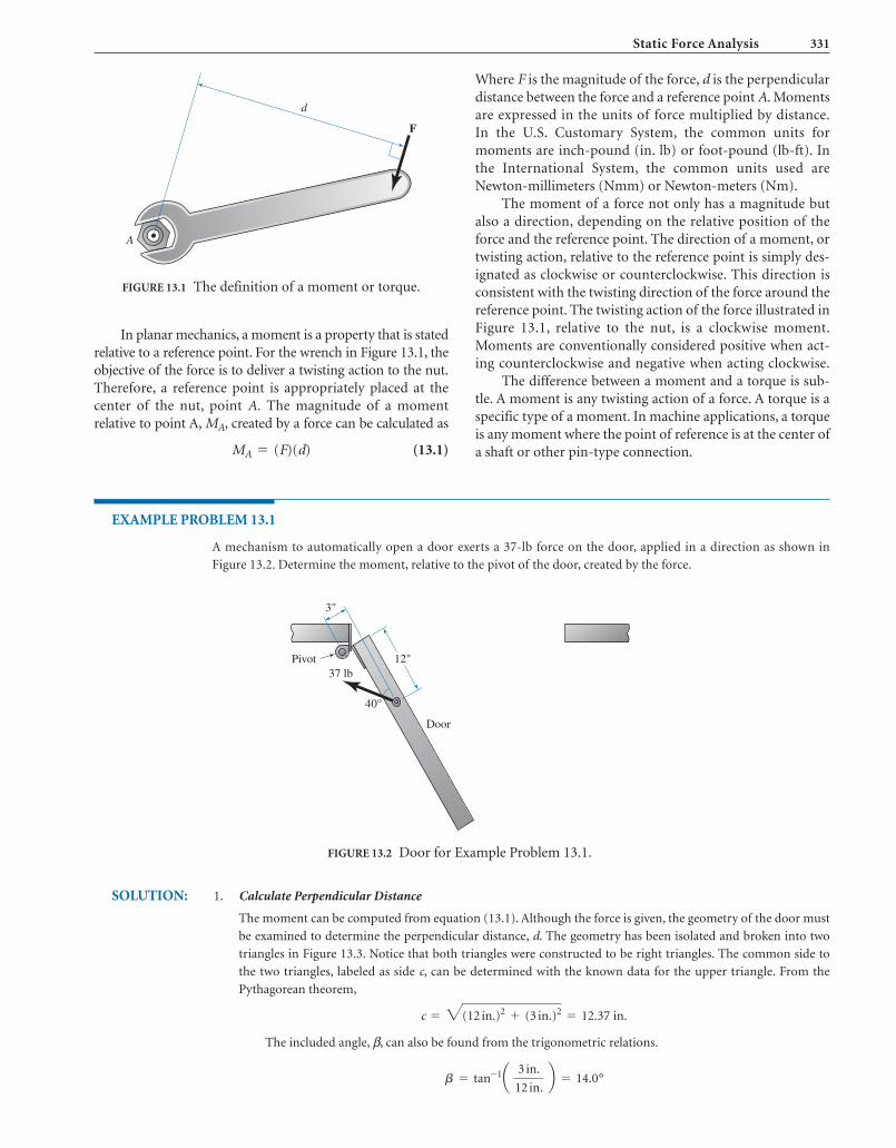
Static Force Analysis 331
d
F
A
FIGURE 13.1 The definition of a moment or torque.
Pivot
Door
3"
12"37 lb
40°
FIGURE 13.2 Door for Example Problem 13.1.
In planar mechanics, a moment is a property that is statedrelative to a reference point. For the wrench in Figure 13.1, theobjective of the force is to deliver a twisting action to the nut.Therefore, a reference point is appropriately placed at thecenter of the nut, point A. The magnitude of a momentrelative to point A, MA, created by a force can be calculated as
(13.1)MA = (F)(d)
Where F is the magnitude of the force, d is the perpendiculardistance between the force and a reference point A. Momentsare expressed in the units of force multiplied by distance.In the U.S. Customary System, the common units formoments are inch-pound (in. lb) or foot-pound (lb-ft). Inthe International System, the common units used areNewton-millimeters (Nmm) or Newton-meters (Nm).
The moment of a force not only has a magnitude butalso a direction, depending on the relative position of theforce and the reference point. The direction of a moment, ortwisting action, relative to the reference point is simply des-ignated as clockwise or counterclockwise. This direction isconsistent with the twisting direction of the force around thereference point. The twisting action of the force illustrated inFigure 13.1, relative to the nut, is a clockwise moment.Moments are conventionally considered positive when act-ing counterclockwise and negative when acting clockwise.
The difference between a moment and a torque is sub-tle. A moment is any twisting action of a force. A torque is aspecific type of a moment. In machine applications, a torqueis any moment where the point of reference is at the center ofa shaft or other pin-type connection.
EXAMPLE PROBLEM 13.1
A mechanism to automatically open a door exerts a 37-lb force on the door, applied in a direction as shown in
Figure 13.2. Determine the moment, relative to the pivot of the door, created by the force.
SOLUTION: 1. Calculate Perpendicular Distance
The moment can be computed from equation (13.1). Although the force is given, the geometry of the door must
be examined to determine the perpendicular distance, d. The geometry has been isolated and broken into two
triangles in Figure 13.3. Notice that both triangles were constructed to be right triangles. The common side to
the two triangles, labeled as side c, can be determined with the known data for the upper triangle. From the
Pythagorean theorem,
The included angle, β, can also be found from the trigonometric relations.
b = tan-1a 3 in.
12 in.b = 14.0°
c = 3(12 in.)2 + (3 in.)2 = 12.37 in.

332 CHAPTER THIRTEEN
A
F1
F2
3"
12"
37 lb
40°
FIGURE 13.4 Force components for Example Problem 13.1.
Focusing on the lower triangle, the included angle, γ, can be found because the total angle was given
as 40°; thus,
Finally, the perpendicular distance can be determined from the trigonometric relations of the lower
triangle.
2. Calculate Moment
The moment, relative to the pivot A, is calculated from equation (13.1). The direction is consistent with the
twisting action of the force relative to the pivot A, which in this case is clockwise.
ALTERNATIVE SOLUTION:
1. Resolve Force into Rectangular Components
In the previous solution, the calculation of a perpendicular distance was rather complex. An alternative solution
can be used that involves defining a convenient coordinate system that is aligned with the given dimensions. The
components of the original force F are identified as F1 and F2 and shown in Figure 13.4.
The magnitude of F1 and F2 can be computed as
MA = F(d ) = 37 lb(5.42 in.) = 200.5 in. lb, cw
d = c sin(g) = (12.37 in.) sin(26°) = 5.42 in.
g = 40° - b = 26°
2. Identify Perpendicular Distance for Each Component
Notice that both of these components cause a moment relative to point A. However, the perpendicular distance
for each moment is apparent. From Figure 13.4, it is seen that the perpendicular distance for F1 and F2 is 12 in.
and 3 in., respectively. Also notice that F1 causes a clockwise turning action around point A. The moment
F2 = (37 lb)cos40° = 28.3 lb
F1 = (37 lb) sin40° = 23.8 lb
c
Pivot A3
d 12
37 1b
40° β
γ
FIGURE 13.3 Door geometry for Example Problem 13.1.

Static Force Analysis 333
3
Fapplied
F34
W
20°
F32y
F32x
FIGURE 13.5 Free-body diagram.
caused by F2 is counterclockwise. The traditional sign convention is to assign counterclockwise moments a
positive value.
3. Calculate Moment
Calculating the moment relative to point A,
= 200.5 in. lb, cw
= -200.5 in. lb
= - [(23.8 lb)(12 in.)] + [(28.3 lb)(3 in.)]
MA = - F1(12 in.) + F2(3 in.)
13.4 LAWS OF MOTION
Sir Isaac Newton developed three laws of motion that serveas the basis of all analysis of forces acting on machines andcomponents. These laws are stated as follows:
FIRST LAW: Every object remains at rest, or moveswith constant velocity, unless an unbalanced force actsupon it.
SECOND LAW: A body that has an unbalanced force has
a. Acceleration that is proportional to the force,
b. Acceleration that is in the direction of the force,and
c. Acceleration that is inversely proportional to themass of the object.
THIRD LAW: For every action, there is an equal andopposite reaction.
All of these laws are utilized in the study of mechanisms.However, in this chapter dealing with static force analysis,only the first and third laws are applicable. The followingchapter incorporates the second law into the analysis.
13.5 FREE-BODY DIAGRAMS
To fully understand the safety of a machine, all forces thatact on the links should be examined. It is widely acceptedthat the best way to track these forces is to construct a free-body diagram. A free-body diagram is a picture of the iso-lated part, as if it were floating freely. The part appears to befloating because all the supports and contacts with otherparts have been removed. All these supports and contacts arethen replaced with forces that represent the action of thesupport. Thus, a free-body diagram of a part shows all theforces acting on the part.
13.5.1 Drawing a Free-Body Diagram
Figure 13.5 illustrates a free-body diagram of an isolatedlink. Notice that this part is designated as link 3. It is essentialthat all forces are shown on the free-body diagram. A conve-nient notation is to label the forces consistent with the linknumber that is being acted upon and the link number that is
driving the action. Thus, a force designated as F34 is a forceon link 3 from the contact of link 4.
Because forces are vectors, determination of a forcerequires knowledge of the magnitude and direction of thatforce. If the direction of a force is known, it should be indi-cated on the free-body diagram. This is the case for F34 inFigure 13.5. When the direction of a force is not known, it iscommon to draw two orthogonal components of theunknown force. These two components represent the twoitems that need to be determined for full understanding ofthe force. Notice that this is the case for F32 in Figure 13.5.
The following steps can assist in systematically drawinga free-body diagram:
I. Isolate the component(s) that must be studied.
II. Draw the component as if it were floating freely inspace by removing all visible supports and physicalcontact that it has with other objects.
III. Replace the supports, or physical contacts, with theappropriate force and/or moments, which have thesame effect as the supports.
13.5.2 Characterizing Contact Forces
Establishing the supporting forces takes some care. As a gen-eral rule, if the nature of the contact prevents motion in acertain direction, there must be a supporting force in that

334 CHAPTER THIRTEEN
F
(a) Direction of Reaction is Known
(b) Direction of Reaction is Unknown
(c) Reaction Prohibits Translation and Rotation
Fy
Fx
Fx
M
Fy
FIGURE 13.6 Reaction forces.
translation in both planar directions. Reactions in thisgroup involve two unknowns, usually shown as the x- and y-components of the reaction force. Figure 13.6billustrates this type of contact.
c. Reaction Prohibits Rotation: Components in thisgroup include fixed supports and pin joints at anactuator (motor or engine). Each of these supports canprevent translation in both planar directions and freerotation. Reactions in this group involve threeunknowns, usually shown as the x- and y-componentsof the reaction force and a reaction moment. Figure13.6c illustrates this type of contact.
EXAMPLE PROBLEM 13.2
An engine hoist is shown in Figure 13.7. The engine being raised weighs 250 lb. Draw a free-body diagram of the
entire hoist.
SOLUTION: In order to construct a free-body diagram of the entire hoist, it first must be isolated and drawn as if it were floating
freely in space. This is done by removing the floor, as it is the only body that supports the hoist. The engine is also
removed, as it is not an integral part of the hoist.
Once the hoist is redrawn without the engine and floor, reaction forces must be placed at the contact points of
the removed items. First, because the engine weighs 250 lb, a force with a known magnitude and direction replaces the
effect of the engine.
Second, the action of the floor must be replicated. The front roller falls into case (a), where the direction of the
reaction force is known. Any roller on a smooth surface prevents translation in a direction perpendicular to the
smooth surface. The reaction at the front roller is labeled .F 21Ay
direction. The types of reactions can be divided into threegroups corresponding to the type of physical contacts.
a. Direction of Reaction is Known: Components inthis group include rollers, sliders, pins in slots, andcables. Each of these supports can prevent motion inonly one direction. Reactions in this group involveonly one unknown, namely the magnitude of thereaction force. Figure 13.6a illustrates this type ofcontact.
b. Direction of Reaction is Unknown: Components inthis group include frictionless pins, hinges, and sliderson rough surfaces. Each of these supports can prevent

Static Force Analysis 335
FIGURE 13.7 Engine hoist for Example Problem 13.2.
250 lb
FED
C
FBDEntire engine hoist
Fx21B
Fy21B
Fy21A
FIGURE 13.8 Free-body diagram for Example Problem 13.2.
The rear roller differs in that a braking device is implemented. In addition to exhibiting a vertical reaction force,
the wheel-and-brake configuration also prevents translation along the floor. Therefore, the reaction at the rear roller
has both x- and y-components. The reactions at the rear roller are labeled and . A completed free-body
diagram is shown in Figure 13.8.
F 21By
F 21Bx
13.6 STATIC EQUILIBRIUM
Newton’s first law applies to all links that are at rest or mov-ing at constant velocity; thus, the condition is referred to asstatic equilibrium. For an object to be in static equilibrium,the following two necessary and sufficient conditions mustbe met:Condition I:The combination, or resultant, of all external forces actingon the object is equivalent to zero and does not cause it totranslate. Mathematically, the first condition of equilibriumcan be summarized as
(13.2)
This condition indicates that all the external forcesacting on the component are balanced. The symbol Σimplies the summation of all forces acting on a free-bodydiagram. As introduced in Chapter 3, forces are vectors andequation (13.2) can be written as
All of the methods for vector manipulation that wereintroduced in Chapter 3 can be used with this vectorequation to solve for unknown forces. Either graphical oranalytical methods can be used, but force analysis is typicallybetter suited for analytical methods. Therefore, the first
F1 + 7 F2 + 7 F3 + 7 Á + 7 FN = 0
© F = 0
condition of static equilibrium can be resolved into compo-nents, yielding two algebraic equations.
(13.3)
(13.4)
Condition II:The moment due to any external force is canceled by themoments of the other forces acting on the object and do notcause it to rotate about any point. The second condition ofequilibrium can be mathematically summarized as
(13.5)
This condition indicates that all the moments acting on thecomponent are balanced. The location of point A is arbitrary.
13.7 ANALYSIS OF A TWO-FORCE MEMBER
A special case of equilibrium, which is of considerable inter-est, is that of a member that is subjected to only two forces.This type of machine component is termed a two-force mem-ber. Many mechanism links, particularly couplers and con-necting rods, are two-force members. A two-force member isshown in Figure 13.9.
©MA = 0
© Fy = 0
© Fx = 0

336 CHAPTER THIRTEEN
FIGURE 13.9 Two-force member.
5 lb 5" 3"
1.5"
1.5"
1"
B
C
1
23
4
A
FIGURE 13.10 Nutcracker for Example Problem 13.3.
2. Act along the same line, and
3. Be opposite in sense.
Because the two forces must act along the same line, the onlyline that can satisfy this constraint is the line that extendsbetween the points where the forces are applied. Thus, a linkwith only two forces simply exhibits either tension orcompression.
This fact can be extremely useful in force analysis. Whenthe locations of the forces are known, the direction of theforces are defined. When the magnitude and sense of a singleforce are known, the other force’s magnitude and sense canbe immediately determined. Thus, the analysis of a two-force member is simple.
EXAMPLE PROBLEM 13.3
A novelty nutcracker is shown in Figure 13.10. A force of 5 lb is applied to the top handle, as shown, and the mecha-
nism does not move (static). Draw a free-body diagram and determine the forces on each link. For this analysis, the
weight of each link can be considered negligible.
SOLUTION: 1. Sketch the Free-Body Diagrams for the Mechanism Links
Notice that link 3 (AC) is a simple link, containing only two pin joints. In addition, no other force is acting on
this link. Thus, it is a two-force member and the forces acting on the link must be equal and along the line
that connects the two pins. The free-body diagram for link 3 is shown as Figure 13.11a. As stated previously, the
notation used is that F32 is a force applied to link 3 as a result of contact from link 2.
Being a two-force member, the direction of the two forces, F34 and F32, is along the line that connects the
two pins. The angle of inclination, θ, of this line can be determined.
Link 2 is also a simple link that contains only two pin joints; however, an additional force is applied to the
handle. Thus, this link is not a two-force member. Newton’s third law stipulates that a force that is acting at A will
be equal and opposite to F32. Thus, the direction of F23 is known as a result of Figure 13.11a. The general pin
joint at point B dictates that two reaction forces will be used. The free-body diagram for link 2 is shown as Figure
13.11b.
Link 4 has sliding contact with link 1. Neglecting any friction force, this contact force will act perpendicu-
lar to the contact surface. The contact force from the nut itself will similarly act perpendicular to the mating
u = tan-1a 2.5
1.5b = 59.0°
In order for a two-force member to be in equilibriumthe two forces must:
1. Have the same magnitude,

Static Force Analysis 337
AA
C
C
B
F23
F32
Fnut
F41
F43
F34
Fx21
Fy21
(b)
(a)
(c)
θθ
θ
1.5"
3"5"
2.5"
1.5"
5 lb
23
4
FIGURE 13.11 Free-body diagrams for Example Problem 13.3.
surface. Also, Newton’s third law stipulates that a force acting at B will be equal and opposite to F34. Thus,
the direction of F43 is known as a result of Figure 13.11a. The free-body diagram for link 4 is shown as
Figure 13.11c.
2. Solve the Equilibrium Equations for Link 2
Link 2 is examined first because it contains the applied force. The three unknown forces on this link
(Figure 13.11b) are solved by using the three equilibrium equations.
Solving the three equations yields
3. Solve the Equilibrium Equations for Link 3
Because link 3 is a two-force member (Figure 13.11a), the equilibrium equations dictate that the forces have the
same magnitude, act along the same line, and are opposite in sense. Of course, Newton’s third law dictates that
. Thus, the forces acting on link 3 are
4. Solve the Equilibrium Equations for Link 4
The free-body diagram of link 4 (Figure 13.11c) will reveal the force exerted on the nut. Of course, Newton’s
third law dictates that . Because the forces on link 4 all converge at a point, the moment equation ofF34 = F43
F34 = 11.96 lb 59°
F32 = 11.96 lb 59°
F32 = F23
F21y
= - 5.25 lb = 5.25 lb T
F21x = - 6.16 lb = 6.16 lb ;
F23 = + 11.96 lb = 11.96 lb 59°
(5 lb)(8 in.) - (F23 cos59.0°) (1.5 in.) - (F23 sin59.0°) (3 in.) = 0
+ ©MB = 0:
F23 sin59.0° + F21y
- 5 lb = 0
+ c ©Fy = 0:
F23 cos59.0° + F21x = 0
+: ©F x = 0:
�
Q
Q b

338 CHAPTER THIRTEEN
equilibrium does not apply. The two unknown forces on this link are solved by using two component
equilibrium equations.
Solving the two equations yields
Fnut = + 10.25 lb = 10.25 lbc
F41 = + 6.16 lb = 6.16 lb:
Fnut - F43 sin59.0° = 0
+c ©Fy= 0:
F41 - F43 cos59.0° = 0
:+ ©Fx
= 0:
EXAMPLE PROBLEM 13.4
Figure 13.12 shows a mechanism used to crush rocks. The 60-mm mechanism crank is moving slowly, and inertial
forces can be neglected. In the position shown, determine the torque required to drive the 60-mm crank and crush the
rocks.
SOLUTION: 1. Sketch Free-Body Diagrams for the Mechanism Links
Using trigonometry to determine the internal angles of this four-bar mechanism can be completed as
discussed in Chapter 4. An alternative approach is to construct the kinematic diagram using CAD. The
internal angles were measured and the results are shown in Figure 13.13. Notice that link 3 (BC) is a simple
link, containing only two pin joints. In addition, no other force is acting on this link. Thus, it is a two-force
member and the forces acting on the link must be equal and along the line that connects the two pins. The
free-body diagram for link 3 is shown as Figure 13.14a. As stated previously, the notation used is that F32 is a
force applied to link 3 as a result of contact from link 2.
Link 2 is also a simple link that contains only two pin joints; however, a drive torque is applied to the
link at the shaft (point A). Thus, this link is not a two-force member. Newton’s third law stipulates that a
force that is acting on link 2 at point B will be equal and opposite to F32. Thus, the direction of F23 is known
as a result of Figure 13.14c. The general pin joint at point A dictates that two reaction forces will be used. The
free-body diagram for link 2 is shown as Figure 13.14b.
360 mm
400 mm
180 mm
90°
130 mm
9000 N
70°
60 mmω
FIGURE 13.12 Rock crusher for Example Problem 13.4.

Static Force Analysis 339
FIGURE 13.13 CAD layout for Example Problem 13.4.
400 mm
F34
F32
(c)
(a)
(b)
180 mm130 mm
70°
9000 N
13.0°
60 mm
3
17.3°
17.3°
65.7°
17.3°
17.3°F23
F43
Fx41
Fy21
Fx21
Fx41
T21
2
4
FIGURE 13.14 Free-body diagrams for Example Problem 13.4.
Link 4 also contains two pin joints but is not a two-force member. The rock-crushing force is applied at a
third point on the link. The angle of this crushing force, from the horizontal, can be calculated from the angles
shown in Figure 13.13. Aligning angles along the horizontal gives
180° - 97.0° - 70° = 13.0°

340 CHAPTER THIRTEEN
Also, Newton’s third law stipulates that a force that is acting onto link 4 at point C will be equal and opposite to
F34. The general pin joint at point D dictates that two reaction forces must be used. The free-body diagram for
link 4 is shown as Figure 13.14a.
2. Solve the Equilibrium Equations for Link 4
Link 4 is examined first because it contains the applied force. The three unknown forces on this link
(Figure 13.11a) are solved by using the three equilibrium equations.
Solving the three equations yields
3. Solve the Equilibrium Equations for Link 3
Because link 3 is a two-force member (Figure 13.14c), the equilibrium equations dictate that the forces have the
same magnitude, act along the same line, and are opposite in sense. Of course, Newton’s third law dictates that
. Thus, the forces acting on link 3 are
4. Solve the Equilibrium Equations for Link 4
The free-body diagram of link 2 (Figure 13.14b) will reveal the instantaneous torque required to operate the de-
vice. Of course, Newton’s third law dictates that .
Solving the three equations yields
Because the torque is the desired value, solving only the moment equation was necessary.
T21 = + 408,561 Nmm = 409 Nm,cw
F21
y= + 2121 N = 212 NT
F21x = + 6809 N = 6809 N;
- T21 + (F23 cos 17.3°) (60 mm) = 0
+ ©M A = 0:
- F21y
+ F23 sin 17.3° = 0
+ c ©F y = 0:
- F21x + F23 cos 17.3° = 0
:+ ©F x = 0:
F23 = F32
F32 = 7132 N 17.3°
F34 = 7132 N 17.3°
F34 = F43
F41y
= + 96.3 N = 96.3 Nc
F41x = + 1960 N = 1960 N;
F43 = + 7132 N = 7132 N 17.3°
(9000 N) (130 mm) - (F43 sin65.7°) (180 mm) = 0
+ ©MD = 0:
(9000 N) sin13.0° - F43 sin17.3° + F41y
= 0
+ c ©F y = 0:
(9000 N)cos13.0° - F43 cos 17.3° - F41x = 0
:+ ©F x = 0:
��
b
b
Q

Static Force Analysis 341
TABLE 13.1 Approximate Coefficients of SlidingFriction
Dry Lubricated
Hard steel On hard steel 0.45 0.08
On Babbitt 0.35 0.15
Mild steel On mild steel 0.60 0.12
On bronze 0.34 0.17
On brass 0.44 —
On copper lead 0.36 0.15
On cast iron 0.23 0.13
On lead 0.95 0.30
On aluminum 0.50 —
On laminated plastic 0.35 0.05
On Teflon — 0.04
Cast iron On cast iron 0.15 0.07
On bronze 0.22 0.07
On brass 0.30 —
On copper 0.29 —
On zinc 0.21 —
Aluminum On aluminum 1.40 —
Output shaft
Follower
3.5"
Scotch-yoke mechanism
Crosshead slot
B
D
CA
Cylinder
Fluid in
300 lb
Piston
135°
FIGURE 13.15 Valve actuator for Example Problem 13.5.
13.8 SLIDING FRICTION FORCE
As stated in Section 13.5, a contact force, as a result of asliding joint, always acts perpendicular to the surface in con-tact. This contact force is commonly referred to as a normalforce because it acts perpendicular to the surfaces in contact.
When friction cannot be neglected in machine analysis,an additional force, friction force, Ff, is observed. Frictionalways acts to impede motion. Therefore, a friction force actson a sliding link, perpendicular to the normal force, and in adirection opposite to the motion (velocity).
For a stationary object, friction works to preventmotion until the maximum attainable friction has beenreached. This maximum value is a function of a coefficient offriction, μ. The coefficient of friction is a property that isdetermined experimentally and is dependent on the materi-als and surface conditions of the contacting links. Averagevalues of friction coefficients for common materials aregiven in Table 13.1. The magnitude of the friction force thatacts on sliding components is calculated as
(13.6)
As mentioned, for moving objects, the friction force actsopposite to the direction of the relative sliding motion.
Ff = mN
EXAMPLE PROBLEM 13.5
The scotch-yoke mechanism shown in Figure 13.15 is used in a valve actuator. As fluid is pumped into the cylinder, the
increased pressure drives the mechanism and applies a torque to the output shaft. This torque can be used to actuate
(open and close) valves. At the instant shown, the pressure load on the piston is 25 lb. Determine the torque generated on
the output shaft. The coefficient of friction between the follower pin and crosshead slot is 0.15.
SOLUTION: 1. Sketch a Kinematic Diagram of the Mechanism
The kinematic diagram of this scotch-yoke mechanism is shown in Figure 13.16.

342 CHAPTER THIRTEEN
2. Sketch Free-Body Diagrams of the Mechanism Links
Link 2 is the piston/rod assembly/crosshead slot. Link 4 is the follower. Notice that link 3 is not a tangible link. It
is used in a kinematic simulation to separate the revolute joint on the follower and the sliding joint in the
crosshead slot. Thus, the mechanism is modeled with all lower-order joints. The kinematic diagram has four
links, two pin joints, and two sliding joints, and consequently one degree of freedom. The driver for this mecha-
nism is the movement of the fluid into the cylinder.
The free-body diagrams for links 2 and 4 are shown in Figure 13.17. Link 3 is not required for force
analysis. Notice that a friction force is shown opposing relative motion. The directions may seem confusing
and warrant further explanation.
Consider link 4 (Figure 13.17b). The pin moves upward relative to the crosshead slot. Therefore, friction
will act to prevent this motion of the pin by acting downward. Similarly, consider link 2 (Figure 13.17a). The slot
moves downward relative to the pin (recall the definition of relative motion). Therefore, friction will act to
prevent this motion of the slot by acting upward.
3. Solve the Equilibrium Equations for Link 2
Link 2 (Figure 13.17a) is examined first because it contains the applied force. For this analysis, only the
x-equilibrium equation is required.
4. Solve the Equilibrium Equations for Link 4
The free-body diagram of link 4 (Figure 13.17b) will reveal the torque on the output shaft. Of course, Newton’s
first law dictates that .
The torque can be determined by using the moment equilibrium equation.
- (F42 cos45°) (3.5 in.) + (mF42 cos45°) (3.5 in.) + T21 = 0
+ ©MA = 0:
Ff42 = mF42 = (0.15)(300 lb) = 45 lb
F42 = F24
F24 = 300 lb;
:+ ©F x = 0:
3.5"
135°B
ACD
2
3
4
FIGURE 13.16 Kinematic diagram for Example Problem 13.5.
3.5"
135°
45°
45° A
(b)(a)
B
T41Fy41
Fx41
F42
4
2
Ff 24 Ff 42
F24F21 C
F21 D
300 lb
FIGURE 13.17 Free-body diagrams for Example Problem 13.5.�

Static Force Analysis 343
β 160 N
100 N
140 N
FIGURE P13.1 Problems 1–3.
25 lb β
8"
FIGURE P13.4 Problems 4–6.
80 mm
50 mm200 N
β
FIGURE P13.7 Problems 7–9.
2.5'
1.5'6'
600 lb
FIGURE P13.10 Problem 10.
Finally, the torque exerted on the output shaft is
T21 = + 631 lb-in. = 631 lb-in., cw
- [(300 lb) cos45°] (3.5 in.) + [(45 lb)cos 45°(3.5 in.)] + T21 = 0
PROBLEMS
Resultant Force
13–1. Determine the resultant for the forces shown inFigure P13.1 when .b = 25°
13–2. Determine the resultant for the forces shown inFigure P13.1 when .
13–3. Determine the resultant for the forces shown inFigure P13.1 when .
Moment of a Force
13–4. A force is applied to a box wrench as shown inFigure P13.4. Determine the moment, relative to thecenter of the nut, when .b = 90°
b = 105°
b = 65°
13–5. A force is applied to a box wrench as shown inFigure P13.4. Determine the moment, relative to thecenter of the nut, when .
13–6. A force is applied to a box wrench as shown inFigure P13.4. Determine the moment, relative to thecenter of the nut, when .b = 110°
b = 75°
13–7. A force that is applied to a control lever is shown inFigure P13.7. Determine the moment, relative to thepivot block, when .b = 0°
13–8. A force that is applied to a control lever is shown inFigure P13.7. Determine the moment, relative to thepivot block, when .
13–9. A force that is applied to a control lever is shown inFigure P13.7. Determine the moment, relative to thepivot block, when .
Static Machine Forces
13–10. Figure P13.10 shows an overhead lift device. If a600-lb force is suspended from the top boom whilethe mechanism is stationary, determine the forcerequired in the cylinder. The top boom weighs 80 lband the weight of the cylinder is negligible.
b = 130°
b = 60°
13–11. Figure P13.11 shows a mechanism that raises pack-ages in a transfer mechanism. If a 100-N package sitson the horizontal link while the mechanism isstationary, determine the torque required from themotor. The weights of the links are negligible.

344 CHAPTER THIRTEEN
13–12. Figure P13.12 shows a mechanism that is used toshear thin-gauge sheet metal. If a 200-N force isapplied as shown, determine the force on the sheetmetal. The weights of the links are negligible.
13–13. Figure P13.13 shows an adjustable platform used toload and unload freight trucks. Currently, a 1200-lbcrate is located as shown. Draw a free-body diagramfor each link. The platform weighs 400 lb, and theweight of all other links is considered insignificant.
13–14. The clamp shown in Figure P13.14 has a rated loadof 1500 lb. Determine the compressive force thiscreates in the threaded rod, AB.
13–15. A utility lift vehicle is shown in Figure P13.15.Determine the force required by the hydraulic cylin-der to maintain the position of the bucket.
13–16. A front loader is shown in Figure P13.16. Determinethe force required from both hydraulic cylinders tomaintain the shovel position.
13–17. A 500-lb crate is supported on a lift table, as shownin Figure P13.17. Determine the force required inthe hydraulic cylinder to keep the platform in theposition shown.
700 mm748 mm
100 mm
400 mm100 N900 mm
FIGURE P13.11 Problem 11.
175 mm
40°30 mm
60 mm
75 mm
100 mm
200 N
FIGURE P13.12 Problem 12.
18"
18"
6"
24" 24" 24"
44"
80"
FIGURE P13.13 Problem 13.
5"
2"
3"
4"
2" 5"
1500 lb
FIGURE P13.14 Problem 14.
2.4 m
5 m
1200 N2.0 m 0.9 m
1.2 m
FIGURE P13.15 Problem 15.
12"
16"
10" 30"
10"20"
15"
50"
12"60"40"
30"
1200 lb
FIGURE P13.16 Problem 16.

Static Force Analysis 345
30"
35"
35"
45" 45"20"
16"
24"
30"
18"
72"
5" 8"
10"
120" 64"
18"
32"
60"
20"
4"
8"
3"
3"
16"
FIGURE P13.19 Problem 19.
J
K
I
H D ECTube
A
B
FIGURE C13.1 (Courtesy, Industrial Press.)
FIGURE P13.17 Problem 17.
FIGURE P13.18 Problem 18.
13–18. Figure P13.18 illustrates a refuse truck capable ofmoving a dumpster from a lowered position, asshown, to a raised and rotated position. Gravityremoves the contents into the truck box. The dump-ster weighs 2400 lb and is shared equally by the twofront forks. Determine the force in the two hydrauliccylinders.
13–19. Figure P13.19 shows a materials handling mecha-nism that slides 8-lb packages along a counter.The coefficient of kinetic friction between thepackage and counter is 0.25. The coefficient ofkinetic friction between the collar and rod is 0.10.
Determine the instantaneous torque required tooperate this mechanism. It operates at a low speed,so inertial forces are negligible.
CASE STUDY
13–1. Figure C13.1 shows a mechanism that gives motionto plunger J. Carefully examine the components ofthe mechanism, then answer the following leading
questions to gain insight into its operation.
1. As lever A is rotated, what type of motion does itemC exhibit?
2. What type of connection do items A and C have?3. What type of motion does ball H have?4. What type of motion does plunger J have?5. What is the purpose of spring K?6. What is the purpose of item E?7. What is the purpose of this mechanism?8. Compare this mechanism to another mechanical
concept that serves the same purpose.

346
C H A P T E R
F O U R T E E N
DYNAMIC FORCE ANALYSIS
chapter deals with force analysis in machines with significantaccelerations. This condition is termed dynamic equilibrium.The analysis of dynamic equilibrium uses many conceptsof static equilibrium. Therefore, an understanding of thetopics presented in the previous chapter is necessary prior tostudying this chapter.
14.2 MASS AND WEIGHT
Mass and weight are not identical. Mass, m, is a measure ofthe amount of material in an object. Mass can also bedescribed as the resistance of an object to acceleration. It ismore difficult to “speed up” an object with a large mass.
The weight, W, of an object is a measure of the pull ofgravity on it. Thus, weight is a force directed toward thecenter of the earth. The acceleration of gravity, g, variesdepending on the location relative to a gravitational pull.Thus, the weight of an object will vary. Mass, however, isa quantity that does not change with gravitational pull.As stated, it is used to describe the amount of material ina part.
The magnitude of weight and mass can be relatedthrough Newton’s gravitational law.
(14.1)
In most analyses on earth, the acceleration of gravity isassumed to be
This assumption is applicable to all machines and mecha-nisms discussed in this book. Of course, in the case ofdesigning machines for use in outer space, a different gravi-tational pull would exist.
Mass and weight are often confused in the U.S.Customary System; it is most convenient to use a derivedunit for mass, which is the slug. This unit directly resultsfrom the use of equation (14.1)
Occasionally, the pound-mass (lbm) is also used as a measureof mass. It is the mass that weighs 1 pound on the surface of
slug = [lb/ft/s2] = lb s2/ft
g = 32.2 ft/s2 = 386.4 in./s2 = 9.81m/s2 = 9810 mm/s2
W = mg
O B J E C T I V E S
Upon completion of this chapter, the student will be able to:
1. Understand the difference between mass and weight.
2. Calculate the mass moment of inertia of an objecteither by assuming a similarity to a basic shape or from the radius of gyration.
3. Transfer the mass moment of inertia to an alternativereference axis.
4. Calculate inertial forces and torques.
5. Determine the forces, including inertia, actingthroughout a mechanism.
14.1 INTRODUCTION
During the design of a machine, determining the operatingforces is critical. Consider the development of an automo-tive windshield wiper system. A key task is the selection ofan electric motor that will drive the wipers. The torquerequired to operate the system is the main attribute in thisselection process. Different scenarios must be considered,such as the fact that the car might be parked under a mapletree. Increased wiper friction due to the tree sap willdemand greater motor torque. A common scenario occursduring periods of heavy rain. The wipers will be operatedon a high-speed setting. As the wipers oscillate at increasedspeeds, large accelerations will result. Inertial forces will becreated from the high accelerations. These forces may belarge enough to damage the components of the wipersystem. In fact, the inertial forces created by the motion ofmany high-speed machines exceed the forces required toperform the intended task. In a reciprocating engine, suchas an automobile engine, the inertial forces can be greaterthan the force produced by the gas pressure. In a gasturbine, the inertial force on the bearings due to an unbal-anced rotor can be magnitudes greater than the weight ofthe rotor.
Thus, for machines with significant accelerations,dynamic force analysis is necessary. The previous chapter dealtwith force analysis in mechanisms without accelerations. This

Dynamic Force Analysis 347
3"
2"
2"10"
cg
4"
0.5"
x
y2"
z
FIGURE 14.1 Part for Example Problem 14.1.
the earth. Assuming that the standard value of gravityapplies, the pound-mass can be converted to slugs by
Generally stated, any calculation in the U.S. CustomarySystem should use the unit of slug for mass. In theInternational System, the common unit used for mass is thekilogram .
14.3 CENTER OF GRAVITY
The center of gravity, cg, of an object is the balance point ofthat object. That is, it is the single point at which theobject’s weight could be held and be in balance in all direc-tions. For parts made of homogeneous material, the cg isthe three-dimensional, geometric center of the object. Formany simple parts, such as a cylinder, the geometric centeris apparent. Locating the center of gravity becomes impor-tant in force analysis because this is the location of the
(kg = N s2/m)
1slug = 32.2 lbm
force of gravity, or weight. In dynamic force analysis, anyinertia effects due to the acceleration of the part will alsoact at this point.
For complex parts, the location of the center of grav-ity is not obvious. A common method of determining thecenter of gravity is to divide the complex part into simpleshapes, where the center of gravity of each is apparent.The composite center of gravity can be determined froma weighted average of the coordinates of the individualcgs. For example, the x-component of the center of gravityof a composite shape can be found from the followingequation:
(14.2)
Because the acceleration due to gravity will be the same forthe entire body, weight can be substituted for mass inequation (14.2). Of course, similar equations can be writtenfor the y- and z-coordinates of the center of gravity.
xcg total =m 1 xcg 1 + m 2 xcg 2 + m 3 xcg 3 + Á
m1 + m2 + m3 + Á
EXAMPLE PROBLEM 14.1
The part shown in Figure 14.1 is made from steel (0.283 lb/in.3). Determine the coordinates of the center of
gravity.
SOLUTION: 1. Divide the Link into Basic Shapes
This part can be readily divided into two components. The lower plate will be designated as component 1, and the
upper shaft will be designated as component 2.
2. Calculate the Weight of the Basic Shapes
The weight of parts is determined by calculating the volume of the parts and multiplying by the density of steel.
These weights and cg coordinates are organized in Table 14.1.
W2 = 10.283 lb/in.32 c p4
(2 in.)2 (3 in.)d = 5.33 lb
W1 = 10.283 lb/in.3 [(10 in.) (4 in.) (0.5 in.)] = 5.66 lb

348 CHAPTER FOURTEEN
14.4 MASS MOMENT OF INERTIA
The mass moment of inertia, I, of a part is a measure of theresistance of that part to rotational acceleration. It is moredifficult to “speed up” a spinning object with a large massmoment of inertia. Mass moment of inertia, or simplymoment of inertia, is dependent on the mass of the objectalong with the shape and size of that object. In addition,inertia is a property that is stated relative to a reference point(or axis when three dimensions are considered). This refer-ence point is commonly the center of gravity of the part.
Figure 14.2 illustrates a general solid object. Notice thata small element of the object has been highlighted. The massmoment of inertia of this small element is determined by
multiplying its mass, dm, by the square of the distance, r, to areference axis, z. This distance is the perpendicular distancefrom the axis to the arbitrary element dm.
The mass moment of inertia of the entire object is thesum of all particles that comprise the object. Mathematically,the moment of inertia is expressed as
(14.3)
Because the definition involves r, the value of the massmoment of inertia is different for each axis. For example,consider a slender rod. The mass moment of inertia relativeto its longitudinal axis will be small because r is smallbecause r is small for each element of the rod. For an axisthat is perpendicular to the rod, the moment of inertia willbe large because r is large for the outermost elements.
Mass moment of inertia is expressed in the units ofmass times squared length. In the U.S. Customary System,the common units are slug-squared feet (slug ft2), whichconvert to pound-feet-squared seconds (lb ft s2). In theInternational System, the common units used are kilogram-squared meters (kg m2).
14.4.1 Mass Moment of Inertia of BasicShapes
Equation (14.2) has been used to derive equations forprimary shapes. Table 14.2 gives these equations, which canbe used to compute the mass moment of inertia forcommon solid shapes of uniform density.
Iz =Lr2 dm
3. Use Equation (14.2) to Calculate the Center of Gravity
The coordinates of the center of gravity are found.
The center of gravity of both parts lies on the z-axis. Therefore, the center of gravity of the composite (total) part
will also lie on the z-axis. Therefore,
zcg total = 0
= (5.66 lb) (0.25 in.) + (5.33 lb) (2 in.)
(5.66 + 5.33) lb = 1.099 in.
ycg total = Wpart 1 ycg part 1 + Wpart 2 ycg part 2
Wpart 1 + Wpart 2
= (5.66 lb) (3 in.) + (5.33 lb) (0 in.)
(5.66 + 5.33) lb = 1.545 in.
xcg total = Wpart 1 xcg part 1 + W part 2 xcg part 2
W part 1 + W part 2
z
z
dmr
FIGURE 14.2 A general solid object.
TABLE 14.1 Basic Shapes Data for Example Problem 14.1
Component Weight (lb) xcg (in.) ycg (in.) zcg (in.)
1 5.66 (10/2 - 2) = 3 (0.5/2) = 0.25 0
2 5.33 0 (0.5/2) = 0.25 0

TABLE 14.2 Mass Moments of Inertia
Shape Name Rendering Mass Moment of Inertia
Cylinder Ix = 1
2 [mr 2]
Iy =1
12 [m(3r 2 + l 2)]
Iz =1
12 [m(3r 2 + l 2)]
Slender rod Ix = 0
Iy =1
12 [ml 2]
Iz =1
12 [ml 2]
Thin diskIx =
1
2 [mr 2]
Iy = 1
4 [mr 2]
Iz = 1
4 [mr 2]
Rectangular block Ix =1
12 [m (w 2 + h 2)]
Iy =1
12 [m (w 2 + l 2)]
Iz =1
12 [m (h2 + l 2)]
Dynamic Force Analysis 349
3" 18" x
FIGURE 14.3 Part for Example Problem 14.2.
EXAMPLE PROBLEM 14.2
The part in Figure 14.3 weighs 3 lb. Determine the mass moment of inertia of the part, relative to an x-axis at the
center of the part.
y
z l x
y
r
x
l
z
y
r
x
z
x
y
lz
h
w
SOLUTION: 1. Determine the Mass of the Part
The part weighs 3 lb and it is assumed to be used on the earth’s surface. The mass can be calculated from
equation (14.1).
m = W
g =
3 lb
32.2 ft/s2 = 0.093 slug

350 CHAPTER FOURTEEN
2. Calculate the Mass Moment of Inertia (Solid Cylinder)
In a true sense, this part is a solid cylinder with
The z-axis in Table 14.2 is equivalent to the x-axis in this analysis. The mass moment of inertia relative to this
axis at the center of the part is
3. Calculate the Mass Moment of Inertia (Slender Rod)
This part may be approximated as a slender rod. Using this assumption, the mass moment of inertia is calculated
from Table 14.2 as
The slender rod assumption underestimates the actual mass moment of inertia by only 1.15 percent. Apparently
this part could be approximated as a slender rod.
= 0.0174slug ft2 = 0.0174 lb ft s2
Ix =1
12[m(l )2] =
1
12[0.093slug (1.5 ft)2]
= 0.0178slug ft2 = 0.0178 lb ft s2
lx =1
12 [m(3r 2 + l 2)] =
1
12 [0.093slug(3(0.125 ft)2 + (1.5 ft)2)]
l = 18 in. = 1.5 ft
r = 1.5 in. = 0.125 ft
14.4.2 Radius of Gyration
Occasionally, the moment of inertia of a part about a spec-ified axis is reported in handbooks using the radius ofgyration, k. Conceptually, the radius of gyration is thedistance from the center of gravity to a point where theentire mass could be concentrated and have the samemoment of inertia.
The radius of gyration can be used to compute the massmoment of inertia by
(14.4)
The radius of gyration is expressed in units of length. Inthe U.S. Customary System, the common units are feet (ft)or inches (in.). In the International System, the commonunits used are meters (m) or millimeters (mm).
I = mk2
14.4.3 Parallel Axis Theorem
Mass moment of inertia is stated relative to an axis.Occasionally, the mass moment of inertia is desired relativeto an alternate, parallel axis. A parallel axis transfer equationhas been derived [Ref. 11] to accomplish this task. To trans-fer the mass moment of inertia from the x-axis to a parallelx′-axis, the transfer equation is
(14.5)
The value d in equation (14.5) is the perpendiculardistance between the two axes. Notice that the second term inequation (14.5) can be either added or subtracted. The termis added when the reference axis is moved away from thecenter of gravity of the basic shape. Conversely, the term issubtracted when the transfer is toward the center of gravity.
Ix œ = Ix ; md2
EXAMPLE PROBLEM 14.3
For the part shown in Figure 14.4, determine the mass moment of inertia of the part relative to an x-axis at the end of
the part.
3" 18"
x′
FIGURE 14.4 Part for Example Problem 14.3.

Dynamic Force Analysis 351
3"
2"
2"10"
4"
0.5"
y2"
FIGURE 14.5 Part for Example Problem 14.4.
SOLUTION: The mass moment of inertia through the center of the part was determined in Example Problem 14.2 as
The distance of the transfer from the center to the end of the part is
Equation (14.5) can be used to transfer the reference axis to the end of the part. Notice that the second term is added
because the transfer is away from the center of gravity.
= 0.0701slug ft2 = 0.0701 lb ft s2
Ix œ = Ix + md 2 = 0.0178slug ft 2 + (0.093 slug) (0.75 ft) 2
d = 9 in. = 0.75 ft
Ix = 0.0178 slug ft2
14.4.4 Composite Bodies
In practice, parts cannot always be simply approximated bythe basic shapes shown in Table 14.2. However, for morecomplex parts, the determination of the moment of inertiacan be done by dividing the complex parts into several basic
shapes from Table 14.2. The mass moment of inertia of eachbasic shape is computed relative to an axis through thecenter of the entire part. Finally, the total mass momentof inertia is determined by combining the values from theindividual shapes.
EXAMPLE PROBLEM 14.4
The part in Figure 14.5 is made from steel. Determine the mass moment of inertia of the part, relative to a y-axis at the
center of the part.
SOLUTION: 1. Identify the Basic Shapes and Determine Their Mass
The part can be divided into two component shapes, as in Example Problem 14.1. Using the weights determined
in that problem, the mass of the two parts is
2. Determine the Centroidal Mass Moment of Inertia of the Basic Shapes
Component 1 is a rectangular block and component 2 is a cylinder. Using Table 14.2, the mass moment of iner-
tia of each part is determined relative to their individual centers of gravity.
Component 1:
= 0.701slug in.2 = 0.0118 slug ft2 = 0.0118 lb ft s2
Iy =1
12[m (w 2 + l 2)] =
1
12[0.176 slug [(4 in.)2 + (10 in.)2]
m2 =W2
g=
5.33 lb
32.2 ft/s2 = 0.165 slug
m1 =W1
g=
5.66 lb
32.2 ft/s2 = 0.176 slug

352 CHAPTER FOURTEEN
Component 2:
3. Utilize the Parallel Axis Theorem
The center of gravity information, determined in Example Problem 14.1, will be used to determine the mo-
ment of inertia for each component relative to the composite center of gravity. The parallel axis theorem is
used to accomplish this. Notice that the perpendicular distance between y-axes is along the x-direction.
Component 1:
Component 2:
4. Calculate the Composite Mass Moment of Inertia
= 10.0162 + 0.00152 slug ft2 = 0.0177slug ft2 = 0.0177 lb ft s2
Iy œ = Iy œ(component 1) + Iy œ(component 2)
= 0.0015slug ft2 = 0.0015 lb ft s2
Iy ¿(component2) = Iy(component2) + m2d22 = 0.0001slug ft2 + 10.165 slug210.0923 ft22
d2 = 11.099 - 02 in. = 1.099 in. = 0.092 ft
= 0.0162slug ft2 = 0.0162 lb ft s2
Iy œ(component 1) = Iy (component 1) + m1d12 = 0.0118slug ft2 + (0.176slug)(0.158 ft)2
d1 = (3.0 - 1.099) in. = 1.901 in. = 0.158 ft
= 0.0138 slug in.2 = 0.0001slug ft2 = 0.0001 lb ft s2
Iy =1
12 [m ( r 2)] (longitudinal axis) =
1
12 [0.165 slug (1 in.)2]
14.4.5 Mass Moment of Inertia—Experimental Determination
One popular experimental method of determining themass moment of inertia of a part is to swing the part as apendulum. This method is illustrated in Figure 14.6.
14.5 INERTIAL FORCE
Section 13.4 listed Newton’s three principal laws of mechan-ics. The second law is critical for all parts that experienceacceleration. It is stated as
SECOND LAW: A body that has an unbalanced force has
a. An acceleration that is proportional to the force,
b. An acceleration that is in the direction of theforce, and
c. An acceleration that is inversely proportional tothe mass of the object.
For linear motion, this law can be stated in terms of theacceleration of the link’s center of gravity, Ag; thus,
(14.7)
Equation (14.7) can be rewritten as
(14.8)
Notice that the subtraction symbol is used becauseboth force and acceleration are vectors.
(- 7 )
© F - 7 mAg = 0
© F = mAg
rcg
FIGURE 14.6 Mass moment of inertia experiment.
If the part is displaced a small angle and released, it willoscillate. The moment of inertia can be determined bymeasuring the time to complete one oscillation, Δt. Themass moment of inertia of the part relative to an axisthrough the center of gravity, has been derived [Ref. 11] as
(14.6)Icg = mrcg c a ¢t
2pb2
g - rcg d

Dynamic Force Analysis 353
1.5"
45 psi
8"
2"
50°
FIGURE 14.7 Mechanism for Example Problem 14.5.
EXAMPLE PROBLEM 14.5
The compressor mechanism shown in Figure 14.7 is driven clockwise by a DC electric motor at a
constant rate of 600 rpm. In the position shown, the cylinder pressure is 45 psi. The piston weighs 0.5 lb, and
the coefficient of friction between the piston and the compressor cylinder is 0.1. The weight of all other
links is negligible. At the instant shown, determine the torque required from the motor to operate the
compressor.
The second term in equation (14.8) is referred to as theinertia of a body. This term is defined as an inertial force,
(14.9)
The negative sign indicates that the inertial force opposesacceleration (it acts in the opposite direction of the accelera-tion). Inertia is a passive property and does not enable abody to do anything except oppose acceleration.
This notion is commonly observed. Imagine pound-ing on the gas pedal in an automobile, violently accelerat-ing the vehicle. Envision the tendency for your head tolurch backward during the acceleration. This is the inertialforce, acting in an opposite direction to the accelerationof the automobile. Further, the extent of the lurch is
Fgi = - 7 mAg
Fgi
proportional to the magnitude of acceleration. Similarly,as the brakes in an automobile are slammed, deceleratingthe vehicle, your head lurches forward, again opposing theacceleration of the automobile. This is Newton’s secondlaw in practice.
Equation (14.8) can be rewritten as
(14.10)
This concept of rewriting equation (14.7) in the form ofequation (14.8) is known as d’Alembert’s principle. Usingd’Alembert’s principle in force analysis is referred to as theinertia–force method of dynamic equilibrium. It allows foranalysis of accelerating links, using the same methods thatare used in a static analysis.
© F + 7 Fgi = 0
SOLUTION: 1. Draw a Kinematic Diagram and Identify the Degrees of Freedom
This is a common in-line, slider-crank mechanism, having a single degree of freedom. A scaled kinematic
diagram is shown in Figure 14.8a.
50°
1
2" A
B
C23 8"
4
(a)
FIGURE 14.8 Diagrams for Example Problem 14.5.
2. Decide on a Method to Achieve the Required Motor Torque
Because the piston is the only component without negligible weight, the inertial force, and the
acceleration, of this component must be determined. The acceleration of the piston (link 4) is strictly
translational and is identical to the motion of point C. Such acceleration analyses have been extensively
presented in Chapter 7.
Once the acceleration of the piston has been obtained, the subsequent inertial forces can be
calculated. Finally, free-body diagrams and the corresponding equations can be used to determine the required
torque.

354 CHAPTER FOURTEEN
(b)
(c)
3. Determine the Velocity of Points B and C
This type of analysis was extensively discussed in the earlier chapters of the book. The 2-in. crank is rotating at
600 rpm. The velocity of point B is
The direction of VB is perpendicular to link 2 and consistent with the direction of ω2, up and to the left. Using
CAD, a vector can be drawn to scale, from the velocity diagram origin, to represent this velocity. The relative
velocity equation for points B and C can be written as
A completed velocity diagram is shown in Figure 14.8b. Scaling the vector magnitudes from the diagram,
VC/B = 82.2 in./s 79°
VC = 80.5 in./s:
VC = VB + 7 VC/B
VB = v2 rAB = 162.8 rad/s212 in.2 = 125.6 in./s 40°
v2 =p
301600 rev/min2 = 62.8 rad/s, cw
FIGURE 14.8 Continued
Q
b

Dynamic Force Analysis 355
4. Calculate Acceleration Components
The next step is to construct an acceleration diagram, which includes points B and C. Calculating the magni-
tudes of the known accelerations,
(directed toward the center of rotation, point A)
(directed from C toward B,measured from CAD)
Note that point A does not have a normal acceleration because the motion is strictly translational.
5. Construct an Acceleration Diagram
The relative acceleration equation for points B and C can be written as
The completed acceleration diagram is shown in Figure 14.8c.
6. Measure the Piston Acceleration
Scaling the vector magnitudes from the diagram,
Because the tangential acceleration of point B is in the same direction as the velocity, the piston is accelerating
(speeding up), not decelerating.
7. Calculate the Inertial Force
Because the piston is the only link of considerable weight, its inertial force is computed by combining equations
(14.9) and (14.1).
Because the piston does not encounter rotational acceleration, rotational inertia is not observed.
8. Sketch Free-Body Diagrams of the Mechanism Links
Notice that link 3 (BC) is a simple link, containing only two pin joints. In addition, no other force is acting on this
link. Thus, it is a two-force member, and the forces acting on the link must be equal and along the line that con-
nects the two pins. The free-body diagram for link 3 is shown as Figure 14.8d. As before, the notation used is that
F32 is a force that is applied to link 3 as a result of contact from link 2.
Link 2 is also a simple link; it contains only two pin joints. However, a moment (torque) is also applied to this
crank. Thus, this link is not a simple, two-force member. Newton’s third law stipulates that a force that is acting at B
will be equal and opposite to F32. Thus, the direction of F23 is known as a result of Figure 14.8d. The angle between
links 2 and 3 was measured from the CAD model. A general pin joint at point A dictates that two reaction forces will
be present. The free-body diagram for link 2 is shown as Figure 14.8e.
Link 4 has sliding contact with link 1. This contact force will act perpendicular to the contact surface. The
force from the compressed gas will, similarly, act perpendicular to the piston surface. A friction force will oppose
the motion (velocity) of link 4. Also, Newton’s third law stipulates that a force that is acting at C will be equal and
opposite to F34. Thus, the direction of F43 is known as a result of Figure 14.8d. The free-body diagram for link 4
is shown as Figure 14.8f.
9. Solve the Dynamic Equilibrium Equations for Link 4
Link 4 is examined first because it contains the applied force. The gas force is calculated as
Fgas = pgas Apiston = pgas c p(dpiston)2
4d = 45 lb/in.2 c p(1.5 in.)2
4d = 79.5 lb;
=(0.5 lb)
386 in./s2 15378 in./s22 = 6.96 lb;
F g 4i = - 7 m4 A g 4 =
W4
g (- 7 A g 4 )
A Ct = 5378 in./s2 :
AC/Bt = 5985 in./s2 79°
ACn + 7 AC
t = ABn + 7 AB
t + 7 AC/Bn + 7 AC/B
t
AC/Bn =
1VC/B22rBC
=182.2 in./s22
8.0 in.= 844 in./s2 11°
aBt = 0 (no angular acceleration of the 2 - in. crank)
ABn =
(VB)2
rAB=1125.6 in./s22
2.0 in.= 7888 in./s2 50°R
a
Q

356 CHAPTER FOURTEEN
The friction force is
The two unknown forces on this link (Figure 14.8f) are solved by using the following equilibrium
equations:
Solving these equations yields
10. Solve for Equilibrium of Link 3
Because link 3 is a two-force member (Figure 14.8d.), the equilibrium equations dictate that the forces have the
same magnitude, act along the same line, and are opposite in sense. Of course, Newton’s third law dictates that
. Thus, the forces acting on link 3 are
11. Solve for Equilibrium of Link 2
The free-body diagram of link 2 (Figure 14.8e) will reveal the required motor torque. Of course, Newton’s third
law dictates that . The unknown forces and moment on this link are solved using the following
equilibrium equations:
-T21 + (F23 sin39°) (2 in.) = 0
+ ©MA = 0:
F 21y + F23 sin11° = 0
+ c ©F y = 0:
F21x - F23 cos11° = 0
:+ ©F x = 0:
F32 = F23
F32 = 89.8 lb 11°
F34 = 89.8 lb 11°
F32 = F23
F41 = +16.6 lb = 16.6 lbc
F43 = +89.8 lb = 89.8 lb 11°
- F43 cos 11.0° + F41 - 0.5 lb = 0
+ c ©F y = 0:
F43 cos 11.0° - Fgas - Fg 4i - Ff = 0
:+ ©F x + 7 F i = 0:
Ff = mF41 = 0.1 F41
R
R
a
�
11°
W = 0.5 lb
C
F41
F ig4
F43
Fgas
Ff 41
4Fx21
T21
Fy21
F23
B
A2"
11°
39°
2
(f)(e)
3
(d)
F32
F34

Dynamic Force Analysis 357
14.6 INERTIAL TORQUE
The concept of an inertial force, as described in equation(14.7), is an extension of Newton’s second law for linearmotion. For rotational motion, the second law can besummarized in terms of rotational acceleration and momentof inertia, relative to an axis through the center of gravity.
(14.11)
Again, the subscript “g” refers to the reference point at thelink’s center of gravity.Similarly to linear motion, equation (14.11) can be rewritten as
(14.12)
Notice that the subtraction symbol is used becausethe directions of the moment and angular acceleration mustbe accounted for. The second term in equation (14.12) is
(- 7 )
© Mg - 7 Tgi = 0
© Mg = Iga
termed the angular inertia of a body. This term is used todefine an inertial torque, :
(14.13)
Again, the negative sign indicates that the inertial torque isdirected opposite to the angular acceleration.Equation (14.12) can be rewritten as
(14.14)
Equation (14.14) is termed the moment equation of dynamicequilibrium. It is the rotational equivalent of d’Alembert’sprinciple described in Section 14.5. It allows for analysis ofaccelerating links, using the same methods as are used in astatic analysis.
The following example problem will combine several ofthe dynamic force analysis concepts presented in this chapter.
© M + 7 Tgi = 0
Tgi = - 7 Iga
Tgi
Solving the three equations yields
Because the torque is the desired value, solving only the moment equation was necessary.
T21 = +113.0 lb in. = 113.0 lb in., cw
F21y
= -17.1 lb = 17.1 lb T
F21x = +88.1 lb = 88.1 lb :
EXAMPLE PROBLEM 14.6
The mechanism shown in Figure 14.9 is used to lower and retract the landing gear on small airplanes. The wheel
assembly link weighs 100 lb, with a center of gravity as shown. The radius of gyration of the assembly, relative to
the center of gravity, has been experimentally determined as 1.2 ft. The motor link is rotating counterclockwise at
3 rad/s and accelerating at 10 rad/s2. For mass property estimation, the motor crank will weigh approximately 15 lb
and will be 2 ft long, 1 ft wide, and 0.25 ft thick. The connecting link is estimated to weigh 20 lb and can be
modeled as a 3.5-ft slender rod. Determine all forces acting on the joints of all links and the torque required to
drive the motor link.
3.0'
3.0'
2.33'
0.75'
2.0'1.77'
30°
FIGURE 14.9 Landing gear for Example Problem 14.6.

2. Decide on a Method to Achieve the Required Motor Torque
Because all links have significant weight, the acceleration of the center of gravity of all links must be determined.
Such acceleration analysis has been extensively presented in Chapter 7. Once the accelerations have been established,
the subsequent inertial forces and torques can be calculated. Finally, free-body diagrams and the corresponding
equations can be used to determine the required torque.
3. Determine the Velocity of Points B and C
This type of analysis was extensively discussed in the earlier chapters of the book. The 1.77-ft crank is rotating at
3 rad/s. The velocity of point B is
The direction of VB is perpendicular to link 2 and consistent with the direction of ω2, up and to the left. Using CAD,
a vector can be drawn to scale, from the velocity diagram origin, to represent this velocity.
The relative velocity equation for points B and C can be written as
The vector diagram is constructed in Figure 14.10b. Scaling the vector magnitudes from the diagram,
4. Calculate Acceleration Components
The next step is to construct an acceleration diagram, which includes points B and C. Calculating the magni-
tudes of the known accelerations,
(directed toward the center of rotation, point A)
(perpendicular to link 2,
consistent with α2)
(directed from C toward B,
measured from CAD)AC/Bn =
(VC/B)2
rBC=
(2.63 ft/s)2
3.0 ft= 2.30 ft/s2 38.6°
ABt = a2 rAB = 110rad/s22 (1.77 ft) = 17.70 ft/s2 60°
ABn =
(VB)2
rAB=15.31 ft/s22
1.77 ft= 15.93 ft/s2 30°
VC/B = 2.63 ft/s 51.4°
VC = 5.00 ft/s 30.7°
VC = VB + 7 VC/B
VB = v2 rAB = 13rad/s2 (1.77 ft) = 5.31 ft/s 60°
358 CHAPTER FOURTEEN
D
.75'
B
A
2.0'1.77'
ω, α.89'
1.5'
(a)
g2
g3
30°
3'
1
2
3
C
3'
2.33'
g4
4
SOLUTION: 1. Draw a Kinematic Diagram and Identify the Degrees of Freedom
This mechanism is the common four-bar linkage, having a single degree of freedom. A kinematic diagram is
given in Figure 14.10a.
Q
Q
R
a
Q
Q

Dynamic Force Analysis 359
(b)
(c)
FIGURE 14.10 Diagrams for Example Problem 14.6.
(directed from C toward D,
measured from CAD)
5. Construct an Acceleration Diagram
The relative acceleration equation for points B and C can be written as
The acceleration polygon is constructed and shown in Figure 14.10c. Notice that the concept of the acceleration
image, as presented in Section 7.10, was used to determine the acceleration of the center of gravity of the three
moving links.
6. Measure the Acceleration of the Center of Gravity of All Links
Scaling the vector magnitudes from the diagram,
AC/Bt = 12.28 ft/s2 51.4° AC
t = 11.60 ft/s2 30.6°
ACn + 7 AC
t = ABn + 7 AB
t + 7 AC/Bn + 7 AC/B
t
ACn =
(VC)2
rCD=
(500 ft/s2)
2.33 ft= 10.72 ft/s2 59.3°a
RQ

360 CHAPTER FOURTEEN
The angular accelerations of the links can then be determined.
7. Calculate Mass Properties
The motor crank can be considered a rectangular block. From Table 14.2, the mass moment of inertia, at the cen-
ter of mass, relative to an axis normal to the broad side of the link is
The connecting arm can be considered a slender rod. From Table 14.2, the mass moment of inertia at the center
of mass relative to an axis normal to the length of the link is
The radius of gyration of the wheel assembly has been experimentally determined. From equation (14.4),
the mass moment of inertia at the center of mass relative to an axis normal to the length of the
assembly is
8. Calculate the Inertial Force
For the three moving links, the inertial force is computed by combining equations (14.9) and (14.1).
9. Calculate the Inertial Torque
For the three moving links, the inertial torque is computed with equation (14.13).
= 2.60 ft lb, cw
Tg 3i = - 7 Ig 3a3 = (0.634 lb ft s2)14.1 rad/s22
= 1.94 ft lb, cw
Tg 2i = - 7 Ig 2a 2 = (0.194 lb ft s2)110rad/s22
=(100 lb)
32.2 ft/s2 120.32 ft/s22 = 63.11 lb 73.4°
Fg 4i = - 7 m4 Ag 4 =
W4
g(- 7 Ag4 )
=(20 lb)
32.2 ft/s2 119.21 ft/s22 = 11.93 lb 89.4°
Fg 3i = - 7 m3Ag 3 =
W3
g(- 7 Ag 3)
=(15 lb)
32.2 ft/s2 111.91 ft/s22 = 5.55 lb 78.0°
Fg 2i - 7 m 2Ag 2 =
W2
g(- 7 Ag 2)
Ig4 = ml2 = a 100 lb
32.2 ft/s2 b (1.2 ft)2 = 4.472 lb ft s2
Ig3 =1
12[ml 2] =
1
12a 20 lb
32.2 ft/s2 b (3.5 ft)2 = 0.634 lb ft s2
Ig2 =1
12[m(W2 + l 2 )] =
1
12a 15 lb
32.2 ft/s2 b [(2 ft)2 + (1 ft)2] = 0.194 lb ft s2
a4 =aC
t
rCD=
11.60 ft/s2
2.33 ft= 5.0 rad/s2, counterclockwise
a3 =aC/B
t
rBC=
12.28 ft/s2
3.0 ft= 4.1 rad/s2, counterclockwise
Ag4 = 20.32 ft/s2 73.4°
Ag2 = 11.91 ft/s2 78.0° Ag3 = 19.21 ft/s2 89.4°
Q
R
R
b
aa

Dynamic Force Analysis 361
10. Sketch Free-Body Diagrams of the Mechanism Links
Because the weight of all links is to be included in the analysis, there are no two-force members. Thus,
all contact forces at the joints are general and are represented by their orthogonal components. The
free-body diagram of link 4 is shown in Figure 14.10d. The free-body diagram of link 3 is shown in Figure
14.10e. Of course, Newton’s third law, declaring that F34 and F43 have the same magnitude and opposing
directions, still applies. Finally, the free-body diagram of link 2 is shown in Figure 14.10f. Because each
link has more than three unknown forces, the equilibrium equations from all links will need to be solved
simultaneously.
11. Generate Equilibrium Equations for Link 4
The following dynamic equilibrium equations are generated from the free-body diagram of link 4
(Figure 14.10d).
- Fg4i [cos(73.4° - 30.6°)] [3.0 ft] - Tg4
i = 0
- F43x [2.33 ft (sin59.4°)] - F43
y [2.33 ft (cos59.4°)] - W4[3.0 ft(cos 59.4°)]
+ ©MD + 7 Tgi = 0:
F 41y - F 43
y - 160.48 lb = 0
F41y - F43
y - W4 - Fg4i sin73.4° = 0
+ c ©F y + 7 Fgi = 0:
F41x - F43
x - 18.03 lb = 0
F41x - F43
x - Fg4i cos 73.4° = 0
:+ ©F x + 7 Fgi = 0:
= 22.36 ft lb, cw
Tg 4i = - 7 Ig 4a 4 = (4.472 lb ft s2)15rad/s22
1.77'
.89'
3.0'
38.6°
89.4°
1.5'
3.0'
2.33'
(f)
(e)
(d)
30°
78°
W2
W3
Fy41
Fx41
Fy43
Fy43
Fy34
Fy32
Fy23
Fy21
Fx34
Fx32
Fx21
Fx23
T21
Fig4
Fig3
Fig2
Tig4
Tig3
Tig2
W4
30.6°
73.4°
59.4°
FIGURE 14.10 Continued
�

362 CHAPTER FOURTEEN
Substituting values gives
12. Generate Equilibrium Equations for Link 3
The following dynamic equilibrium equations are generated from the free-body diagram of link 3
(Figure 14.10e).
Substituting values gives
13. Generate Equilibrium Equations for Link 2
The following dynamic equilibrium equations are generated from the free-body diagram of link 2
(Figure 14.10f).
Substituting values gives
14. Solve the Equilibrium Equations
A total of nine equilibrium equations have been generated. As previously stated, Newton’s third law stipulates
that the following magnitudes are equal.
F23x = F32
x F 23y = F23
y
F43x = F34
x F 43y = F 34
y
T21 + 0.885 F23x + 1.533 F 23
y - 17.17 ft lb = 0
Fg 2i [sin(78° - 30°)] [0.89 ft] - Tg 2
i = 0
T21 + F23x [1.77 ft (sin 30°)] + F23
y[1.77 ft (cos30°)] - W2 [0.89 ft (cos30°)]
+ ©MA + 7 Tgi = 0:
F23y + F21
y - 20.43 lb = 0
F23y + F21
y - W2 - Fg 2i sin78° = 0
+ c ©Fy + 7 Fgi = 0:
F23x + F 21
y + 1.15 lb = 0
F23x + F21
x + Fg 2i cos78° = 0
:+ ©Fx + 7 Fgi = 0:
2.344 F34x - 1.872 F 34
y + 34.95 ft lb = 0
+ Fg 3i [cos (38.6° - 0.6°)] [1.5 ft] - Tg 3
i = 0
F34x [3.0 ft (cos 38.6°)] - F34
y [3.0 ft (sin38.6°)] (2.33 ft) + W3 [1.5 ft (cos38.6°)]
+ ©MB + 7 Tgi = 0:
F34y - F32
y - 31.93 lb = 0
F34y - F32
y - W3 - Fg3i sin89.4° = 0
+c ©F y + 7 Fgi = 0:
F34x - F32
x - 0.13 lb = 0
F 34x - F32
x - Fg 3i cos89.4° = 0
:+ ©F x + 7 Fgi = 0:
- 2.000 F43x - 1.186 F43
y - 313.98 ft lb = 0
��

Dynamic Force Analysis 363
Ld
δ
FIGURE P14.9 Problems 9 and 10.
L
d
Longitudinal axis
Axis perpendicular to length
y0.75"
0.75"
3.25"1.75"
0.125"
Ø 0.375"
Ø 0.375"
FIGURE P14.5 Problems 5–8.
FIGURE P14.11 Problem 11.
PROBLEMS
Mass and Mass Moment of Inertia
14–1. The mass of a connecting rod from an internalcombustion engine has been determined to be2.3 kg. Compute the weight of the rod.
14–2. A robotic gripper was weighed at 4.5 lb. Determinethe mass of the gripper.
14–3. A robotic gripper was weighed at 4.5 lb and has aradius of gyration relative to a certain axis at the centerof gravity of 5 in. Determine the mass moment of iner-tia of the part relative to this axis.
14–4. A 6-kg mechanism link has a radius of gyrationrelative to a certain axis at the center of gravity of150 mm. Determine the mass moment of inertia ofthe part relative to this axis.
14–5. For the part shown in Figure P14.5, calculate themass moment of inertia and the radius of gyrationabout a centroidal longitudinal axis of a 14-in.-longshaft that weighs 5 lb and has a diameter of 0.625 in.
14–6. For the part shown in Figure P14.5, calculate the massmoment of inertia and the radius of gyration about acentroidal longitudinal axis of a 1200-mm-long shaftthat has a mass of 100 kg and a diameter of 50 mm.
14–7. The part shown in Figure P14.5 is a solid cylinder 2 ftin diameter, 3 ft long, and weighing 48 lb. Determine
the mass moment of inertia about its centroidal axialaxis.
14–8. The part shown in Figure P14.5 is a solid cylinder 2 ftin diameter, 3 ft long, and weighing 48 lb. Determinethe mass moment of inertia about a centroidal axis,perpendicular to its length.
14–9. The part shown in Figure P14.9 is a slender rod, 14in. long, rotating about an axis perpendicular to itslength and 3 in. from its center of gravity. Knowingthat the rod weighs 2 lb and has a diameter of1.25 in., determine its mass moment of inertiaabout that axis.
14–10. The part in Figure P14.9 is a slender rod, 0.4 m long,rotating about an axis perpendicular to its lengthand 0.12 m from its center of gravity. Knowing thatthe rod has a mass of 6 kg, determine its massmoment of inertia about that axis.
14–11. Determine the moment of inertia of the steel linkshown in Figure P14.11 with
respect to the y-axis.(r = 0.183 lb/in.3)
Therefore, nine unknown quantities remain. Solving the nine equilibrium equations, simultaneously, gives the
following results:
T21 = + 307.88 ft lb = 307.88 ft lb, cw
F21y = + 154.46 lb = 154.46 lbc
F21x = + 95.17 lb = 95.17 lb:
F32y = - 134.03 lb = 134.03 lbc and F23
y = 134.03 lbT
F32x = - 96.32 lb = 96.32 lb: and F23
x = 96.32 lb;F43
y = - 102.09 lb = 102.09 lbc and F34y = 102.09 lbT
F43x = - 96.44 lb = 96.44 lb: and F 34
x = 96.44 lb;F41
y = + 58.38 lb = 58.38 lbc
F41x = - 78.41 lb = 78.41 lb;
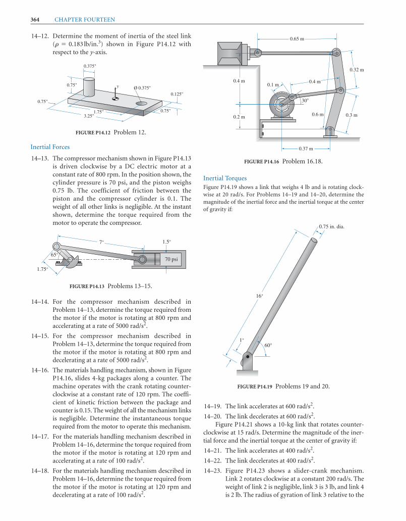
364 CHAPTER FOURTEEN
16"
1"60°
0.75 in. dia.
FIGURE P14.19 Problems 19 and 20.
0.2 m
0.4 m
0.37 m
30�
0.6 m 0.3 m
0.32 m
0.65 m
0.4 m0.1 m
FIGURE P14.16 Problem 16.18.
14–12. Determine the moment of inertia of the steel linkshown in Figure P14.12 with
respect to the y-axis.(r = 0.183 lb/in.3)
Inertial Forces
14–13. The compressor mechanism shown in Figure P14.13is driven clockwise by a DC electric motor at aconstant rate of 800 rpm. In the position shown, thecylinder pressure is 70 psi, and the piston weighs0.75 lb. The coefficient of friction between thepiston and the compressor cylinder is 0.1. Theweight of all other links is negligible. At the instantshown, determine the torque required from themotor to operate the compressor.
14–14. For the compressor mechanism described inProblem 14–13, determine the torque required fromthe motor if the motor is rotating at 800 rpm andaccelerating at a rate of 5000 rad/s2.
14–15. For the compressor mechanism described inProblem 14–13, determine the torque required fromthe motor if the motor is rotating at 800 rpm anddecelerating at a rate of 5000 rad/s2.
14–16. The materials handling mechanism, shown in FigureP14.16, slides 4-kg packages along a counter. Themachine operates with the crank rotating counter-clockwise at a constant rate of 120 rpm. The coeffi-cient of kinetic friction between the package andcounter is 0.15. The weight of all the mechanism linksis negligible. Determine the instantaneous torquerequired from the motor to operate this mechanism.
14–17. For the materials handling mechanism described inProblem 14–16, determine the torque required fromthe motor if the motor is rotating at 120 rpm andaccelerating at a rate of 100 rad/s2.
14–18. For the materials handling mechanism described inProblem 14–16, determine the torque required fromthe motor if the motor is rotating at 120 rpm anddecelerating at a rate of 100 rad/s2.
Inertial TorquesFigure P14.19 shows a link that weighs 4 lb and is rotating clock-wise at 20 rad/s. For Problems 14–19 and 14–20, determine themagnitude of the inertial force and the inertial torque at the centerof gravity if:
1.5"
70 psi
7"
1.75"
65°
FIGURE P14.13 Problems 13–15.
y0.75"
0.75"
3.25"1.75"
0.125"Ø 0.375"
0.375"
0.75"
FIGURE P14.12 Problem 12.
14–19. The link accelerates at 600 rad/s2.
14–20. The link decelerates at 600 rad/s2.Figure P14.21 shows a 10-kg link that rotates counter-
clockwise at 15 rad/s. Determine the magnitude of the iner-tial force and the inertial torque at the center of gravity if:
14–21. The link accelerates at 400 rad/s2.
14–22. The link decelerates at 400 rad/s2.
14–23. Figure P14.23 shows a slider-crank mechanism.Link 2 rotates clockwise at a constant 200 rad/s. Theweight of link 2 is negligible, link 3 is 3 lb, and link 4is 2 lb. The radius of gyration of link 3 relative to the
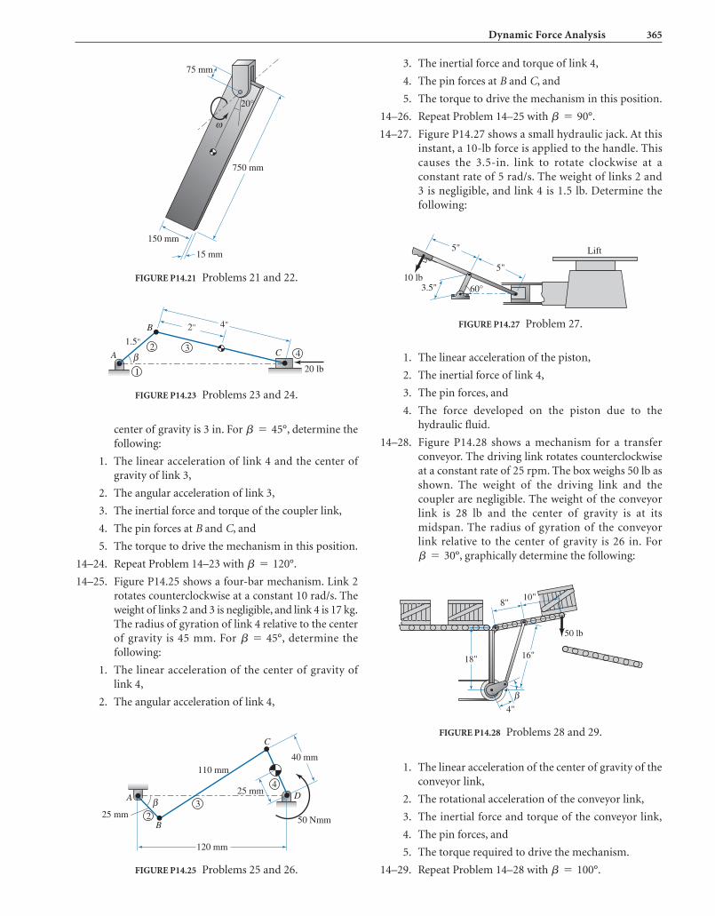
Dynamic Force Analysis 365
C
D
40 mm
25 mm
50 Nmm
120 mm
110 mm
B
A
25 mmβ 3
2
4
FIGURE P14.25 Problems 25 and 26.
5"
5"10 lb
3.5"
Lift
60°
FIGURE P14.27 Problem 27.
8"10"
50 lb
16"18"
4"
β
FIGURE P14.28 Problems 28 and 29.
150 mm
15 mm
750 mm
ω
75 mm
20°
FIGURE P14.21 Problems 21 and 22.
32
1
4A
B
1.5"
β C
2" 4"
20 lb
FIGURE P14.23 Problems 23 and 24.
center of gravity is 3 in. For , determine thefollowing:
1. The linear acceleration of link 4 and the center ofgravity of link 3,
2. The angular acceleration of link 3,
3. The inertial force and torque of the coupler link,
4. The pin forces at B and C, and
5. The torque to drive the mechanism in this position.
14–24. Repeat Problem 14–23 with .
14–25. Figure P14.25 shows a four-bar mechanism. Link 2rotates counterclockwise at a constant 10 rad/s. Theweight of links 2 and 3 is negligible, and link 4 is 17 kg.The radius of gyration of link 4 relative to the centerof gravity is 45 mm. For , determine thefollowing:
1. The linear acceleration of the center of gravity oflink 4,
2. The angular acceleration of link 4,
b = 45°
b = 120°
b = 45°
3. The inertial force and torque of link 4,
4. The pin forces at B and C, and
5. The torque to drive the mechanism in this position.
14–26. Repeat Problem 14–25 with .
14–27. Figure P14.27 shows a small hydraulic jack. At thisinstant, a 10-lb force is applied to the handle. Thiscauses the 3.5-in. link to rotate clockwise at aconstant rate of 5 rad/s. The weight of links 2 and3 is negligible, and link 4 is 1.5 lb. Determine thefollowing:
b = 90°
1. The linear acceleration of the piston,
2. The inertial force of link 4,
3. The pin forces, and
4. The force developed on the piston due to thehydraulic fluid.
14–28. Figure P14.28 shows a mechanism for a transferconveyor. The driving link rotates counterclockwiseat a constant rate of 25 rpm. The box weighs 50 lb asshown. The weight of the driving link and thecoupler are negligible. The weight of the conveyorlink is 28 lb and the center of gravity is at itsmidspan. The radius of gyration of the conveyorlink relative to the center of gravity is 26 in. For
, graphically determine the following:b = 30°
1. The linear acceleration of the center of gravity of theconveyor link,
2. The rotational acceleration of the conveyor link,
3. The inertial force and torque of the conveyor link,
4. The pin forces, and
5. The torque required to drive the mechanism.
14–29. Repeat Problem 14–28 with .b = 100°

366 CHAPTER FOURTEEN
mechanism, then answer the following leadingquestions to gain insight into its operation.
1. As gear A rotates clockwise, describe the motion ofgear B.
2. As gear A rotates clockwise, what is the immediatemotion of slide C?
3. Discuss the action that takes place as pin E reachesthe end of the slot.
4. Discuss precisely the continual motion of slides Cand E.
5. Discuss how this motion could possibly be used in awire-stripping machine.
6. What is the purpose of spring G?
7. How would the mechanism change if a “stiffer”spring were installed?
CASE STUDY
C14–1 Figure C14.1 shows a mechanism that gives motionto slides C and D and is used in a wire-strippingmachine. Carefully examine the components of the
C E
A
G
D
B
F
FIGURE C14.1 (Courtesy, Industrial Press.)

ANSWERS TO SELECTED EVEN-NUMBERED PROBLEMS
Chapter 11–26.
1–28.
1–30.
1–32.
1–34.
1–36.
1–38.
1–40.
1–42.
1–44.
1–46.
1–48.
1–50.
1–52. Crank-rocker
1–54. Crank-rocker
Chapter 33–2.
3–4.
3–6.
3–8.
3–10.
3–12.
3–14.
3–16.
3–18.
3–20.
3–22.
3–24.
3–26.
3–28.
3–30.
3–32.
3–34.
3–36.
3–38.
3–40.
3–42.
3–44.
3–46.
3–48.
3–52.
3–54.
3–56. J = 101.68 18.3°
J = 109.8 24.1°
J = 26.10 11.4°
J = 101.68 18.3°
J = 109.76 24.1°
J = 26.094 11.4°
J = 212.13 65.0°
J = 5.587 13.8°
J = 8.074 68.3°
J = 212.13 65.0°
J = 5.587 13.76°
J = 8.074 68.3°
R = 221.2 13.4°
R = 212.13 25.0°
R = 24.18 18.1°
R = 221.20 13.5°
R = 212.13 25.0°
R = 24.18 18.1°
h = 83.1 in.
y = 11.7 ft
h = 11.3 ft
L = 8 ft, 8 in.
s = 175 mm
x = 11.5 in. y = 16.4 in.
s = 156.6 mm
R = 12 in.
A = 17.3 in.
n = 6, jp = 7, jh = 0, M = 1
n = 8, jp = 10, jh = 0, M = 1
n = 4, jp = 4, jh = 0, M = 1
n = 9, jp = 11, jh = 0, M = 2
n = 6, jp = 7, jh = 0, M = 1
n = 6, jp = 7, jh = 0, M = 1
n = 6, jp = 7, jh = 0, M = 1
n = 4, jp = 4, jh = 0, M = 1
n = 4, jp = 4, jh = 0, M = 1
n = 6, jp = 7, jh = 0, M = 1
n = 4, jp = 4, jh = 0, M = 1
n = 4, jp = 4, jh = 0, M = 1
n = 4, jp = 4, jh = 0, M = 1
3–58.
3–60.
3–62.
Chapter 44–2.
4–4.
4–6.
4–8.
4–10.
4–12.
4–14.
4–16.
4–18.
4–20.
4–22.
4–24.
4–26.
4–28.
4–30.
4–32.
4–34.
4–36.
4–38.
4–40.
4–42.
4–44.
4–46.
4–48.
4–50.
4–52.
4–54.
4–56.
4–58.
4–60.
4–62.
4–64.
4–66.
4–68.
Chapter 55–2.
5–4.
5–6.
5-8.
5-10. Q = 2.083, v = 162.2 rpm
Q = 1.714, v = 63.2 rpm
t1 = 0.067 s, t2 = 0.53 s
t1 = 0.188s, t2 = 0.142 s
b = 49.1°, v = 109 rpm
(¢Rslide pin)max = 44.50 mm
(¢uwiper arm)max = 72.8°
(¢Rblade)max = 1.513 in.
(¢uram)max = 29.5°
(¢uwheel assy)max = 57.6°
(¢uram)max = 46.3°
(¢Rpiston)max = 90.0 mm
¢uram = 5.5°, cw
¢Rclaw = 30.87 mm 86.52°
¢Rbox = 0.362 mT¢L cylinder = 68.1 mm, shorter
¢utop handle = 16.8°, cw
¢uram = 14.4°, cw
¢Rstamp = 1.570 in.T¢Rpiston = 66.82 mm;¢RP = 7.247 10.0°
¢ubed = 14.0°, ccw
¢uram = 3.03°, cw
¢Lspring = 1.118 in., shorter
¢Rclaw = 29.62 mm 85.2°
¢Lcylinder = 1.566 in.
¢Rbox = 0.579 mT¢Rcarrier = 249.7 mm 45.5°
¢Rend = 203.4 73.9°
¢uwheel = 16.3°, cw
¢uhandle = 34.4°, ccw
¢Rend = 22.644 in. 44.9°
¢uram = 17.6°, ccw
¢uhandle = 22.2°, ccw
¢Rend = 2.029 in. 55.1°
¢ucrank = 23.0°, ccw
¢Rpiston = 47.10 mm;¢RP = 8.420 in. 27.5°
¢x = 2.189 in.:
D = 38.12 F = 238.9
B = 8.81 C = 117.7
C = 19.22 E = 17.52
367
a b b
Q
Q
Q
b
b
b b
b
b R
R
R
R
R
a
Q
Q
b
b
R
a
a
a

5–12.
5–14.
5–16.
5–18.
5–20.
5–22.
5–24.
5–26.
5–28.
5–30.
5–32.
Chapter 66–2.
6–4.
6–6.
6–8.
6–10.
6–12.
6–14.
6–16.
6–18.
6–20.
6–22.
6–24.
6–26.
6–28.
6–30.
6–32.
6–34.
6–36.
6–38.
6–40.
6–42.
6–44.
6–46.
6–48.
6–50.
6–74.
6–76.
6–78.
6–80.
6–82.
6–84.
6–86.
6–88.
6–90.
6–92.
6–94.
Chapter 77–4.
7–6. acam = 9.82 rad/s2, cw
¢RA = 40 mm c
V-2. Avehicle = 10.60 ft/s2
VCylinder = 2.64 in./s, compressing
vsegment gear = 5.421 rad/s, cw
vwiper arm = 31.46 rad/s, cw
Vblade = 91.11 in./s:Vplatform = 12.79 ft/min 12.9°
Vright piston = 288.3 in./s 45°vblade = 0.071 rad/s, ccw
vbath = 1.245 rad/s, cw
Vblade = 4.82 in./sTVpiston = 230.3 in./s;Vpackage = 953 mm/s:Vcylinder = 4.39 in./s, compressing
vsegment gear = 3.827 rad/s, cw
vwiper arm = 1.88 rad/s, cw
Vblade = 112.64 in./s:Vplatform = 15.99 ft/min 12.9°
Vpackage = 775 mm/s:Vright piston = 150.68 in./s 45°
Vcylinder = 4.39 in./s, compressing
Vblade = 112.91 mm/scvsegment gear = 2.232 rad/s, ccw
vbath = 0.85 rad/s, cw
vwiper blade = 2.50 rad/s, ccw
Vblade = 5.94 in./sTVblade = 59.63 in./s;Vpiston = 272.55 in./s;VA/B = 15.72 ft/s 25.9°
VB/A = 5.94 ft/s 59.4°
VB = 90 ft/s 20°
V = 125.66 ft/min
¢Rtotal = 7.5 in.
¢Rtotal = 72 in.
vmin = .0167 rpm
v = 22.37 min/hr
¢t = 37.5 s
b = 51.43°, v = 240 rpm
b = 49.09°, v = 17.6 rpm
b = 6.92°, v = 40 rpm
b = 8.57°, v = 300 rpm
b = 16.36°, v = 200 rpm
b = 19.3°, v = 33.3 rpm
b = 0°, v = 17.14 rpm
b = 8.6°, v = 1818 rpm
b = 12.6°, v = 4286 rpm
b = 20°, v = 100 rpm
L2 = 4 mm, v = 750 rpm 7–8.
7–10.
7–12.
7–14.
7–16.
7–18.
7–20.
7–22.
7–24.
7–26.
7–28.
7–30.
7–32.
7–34.
7–36.
7–38.
7–40.
7–42.
7–44.
7–60.
7–62.
Chapter 8(spreadsheet/program results at shown at 120° crank angle)
8–2.
8–4.
8–6.
8–8.
8–10.
8–12.
Chapter 99–14.
9–16.
9–18.
9–20.
9–22.
9–28.
9–30.
9–32.
9–34.
9–36.
9–62.
Chapter 1010–2.
10–4.
10–6.
10–8.
10–10.
10–12.
10–14. C = 3.5 in.
D1 = 2 in., D2 = 4.5 in.
C = 1.125 in.
mp = 1.47
mp = 1.53
D = 84 mm
p = 0.393 in.
vout = 7.46 rad/s, aout = 123 rad/s2
Vmax = 1.43 in./s, Amax = 6.41 in./s2
Vmax = 189 mm/s, Amax = 2961 mm/s2
Vmax = 8.0 mm/s, Amax = 8.0 mm/s2
Vmax = 1.25 in./s, Amax = 3.13 in./s2
vcam = 9.4 rpm, Vmax = 0.94 in./s
vcam = 20 rpm, Vmax = 2.0 in./s
vcam = 17.1 rpm, Vmax = 3.1 in./s
vcam = 13.3 rpm, Vmax = 2.5 in./s
vcam = 42.9 rpm, Vmax = 4.0 in./s
vcam = 10.9 rpm, Vmax = 0.5 in./s
v4 = 204.4 rad/s at u2 = 120°
A4 = 2349 mm/s2 at u2 = 120°
v4 = 3.27 rad/s at u2 = 120°
V4 = -2577 mm/s at u2 = 120°
u4 = 16.6° at u2 = 120°
¢R4 = 123.9 mm at u2 = 120°
AcB3/B2 = 900 mm/s2 60°
AcB3/B2 = 900 mm/s2 30°
Apiston = 93,195 in./s2:awheel assy = 2.08 rad/s2, cw
anozzle = 78.55 rad/s2, cw
anozzle = 9.80 rad/s2, ccw
ahorse = 5.22 rad/s2, cw
Ablade = 103.73 in./s2;Ablade = 58.97 in./s2;Aneedle = 29,271 mm/s2cApiston = 37,194 in./s2:Apiston = 31,341 in./s2:AC/B = 1.35 ft/s2 42.3°
AA/B = 25.46 mm/s2 11.3°
AA = 5158 in./s2 6.9°
AB = 22,872 in./s2 71.0°
AnB = 17,770 in/s2 70°
¢Ractuator = 10 in.
¢Rlinear motor = 15 in.T¢Ractuator = 85 in.
ashaft = 7.85 rad/s2, cw
368 Answers to Selected Even-Numbered Problems
Q
Q
Q
b
b
b
b
R
R a a
a
a
Q

10–16.
10–18.
10–20.
10–22.
10–24.
10–26.
10–28.
10–30.
10–32.
10–34.
10–36.
10–38.
10–40.
10–42.
10–44.
10–46.
10–48.
10–50.
10–52.
10–54.
10–56.
10–58.
10–60.
10–62.
10–64.
10–66.
10–68.
10–70.
10–72.
Chapter 1111–2.
11–4.
11–6.
11–8.
11–10.
11–12.
11–14.
11–16.
11–18.
11–20.
11–22.
11–24.
11–26.
11–28. No. 100 Chain
No. 80 Chain
c = 52.424 in., u = 96°
c = 48.724 in., u = 125°
vin. = 760 rpm, cw
vout = 84 rpm, cw
3V belt
3V belt
5V belt
c = 25.618 in., u = 144°
c = 22.375 in., T = 162°
vin = 2700 rpm, ccw
vout = 313 rpm, ccw
vout = 479 rpm, cw
v8 = 378 rpm, ccw
v6 = 536 rpm, cw
v4 = 2160 rpm, cw
¢uwindow = 10.8°ccw
¢uwindow = 8°ccw
N = 17-68, 17-68, 18-45, 18-45, 17-34
v1 = 2520 rpm, C = 9 in.
v1 = 3576 rpm
Pd = 8
s4 = 0.74 in., c = 4.625 in.
v8 = 30 rpm, cw; C = 17.97 in.
v5 = 100 rpm, cw; c = 8.5 in.
Pd = 12, Nw = 2, Ng = 50, l = 5°
gp = 10.4°, gg = 64.6°
gp = 14.9°, gg = 75.1°
Pd = 7.6, N1 = 19, N2 = 38
pn = 0.28 in.
v = 10.6 rpm
¢s = 42.4 in.
¢u = 2.12 rev
Pd = 12, D1 = 4.0 in., D2 = 24.0 in.
D1 = 2.0 in., D2 = 10.25 in.
D1 = 3.0 in., D2 = 13.33 in.
Pd = 12
Pd = 4, N1 = 20, N2 = 60
Pd = 8, N1 = 16, N2 = 64
N1 = 24 teeth, N2 = 96 teeth
Vt = 90.3 in./s
Vt = 67.7 in./s Chapter 1212–2.
12–4.
12–6.
12–8.
12–10.
12–12.
12–14.
12–16.
12–18.
12–20.
12–22.
12–34.
12–36.
12–38.
12–40.
Chapter 1313–2.
13–4.
13–6.
13–8.
13–10.
13–12.
13–14.
13–16.
13–18.
Chapter 1414–2.
14–4.
14–6.
14–8.
14–10.
14–12.
14–14.
14–16.
14–18.
14–20.
14–22.
Tcgi = 19.5 Nm, ccw
Fcgi = 1377 N 49.4°
T cgi = 132.5 in. lbs, cw
Fcgi = 52.25 lbs 3.7°
Tmotor = 10.22 Nm, ccw
Tmotor = 14.04 Nm, ccw
Tmotor = 199.49 in. lbs, cw
Iy cg = 0.00626 lb in. s2
Iz = 0.166 kg m2
Iz = 1.49lb ft s2
Ix = 31.25 kg m2
I = 0.135 kg m2
m = 0.14 slugs
Rear cyl = 11,110 lbs(C)
Front cyl = 5000 lbs(T)
Rear cyl = 7182 lbs(C)
Front cyl = 2137 lbs(C)
Fscrew = 1200 lb(C)
Fmetal = 868 NTFcyl = 3733 lbs(C)
M = 18.9 Nm, cw
M = 188 in. lbs, cw
M = 200 in. lbs, cw
R = 248 66°
M10 * 1.50 and M8 * 1.25
e = 24.5%
e = 47.2%
e = 26%
Vplatform = 7.236 in./s 32.8°
Vtable = 0.154 in./scVnut = 0.167 in./sT¢Rfront end = 0.921 in. 86.7°
¢Rend = 6.445 in. 28.3°
¢Rplatform = 2.564 in. 29.7°
¢Rplate = 2.756 in.T¢Rtable = 0.154 in.c¢Rram = 2.5 in.cp = .020 in., l = 3.65°
p = .0357 in., l = 2.87°
Answers to Selected Even-Numbered Problems 369
Q
Q Q
Q
Q
b
R

370
REFERENCES
1. Barton, Lyndon, Mechanism Analysis: Simplified Graphicaland Analytical Techniques, 2nd ed., Marcel Dekker Inc.,New York, 1993.
2. Baumeister, Theodore III, Avallone, Eugene, and Sadegh,Ali, Mark’s Standard Handbook for Mechanical Engineers,11th ed., McGraw-Hill Book Company, New York, 2006.
3. Chironis, Nicholas and Sclater, Neil, Mechanisms andMechanical Drives Sourcebook, 4th ed., McGraw-Hill BookCompany, New York, 2007.
4. Erdman, Aurthur, Sandor, George, and Kota, Sridhar,Mechanism Design, Vol 1: Analysis and Synthesis, 4th ed.,Prentice Hall, Upper Saddle River, NJ, 2001.
5. Kepler, Harold, Basic Graphical Kinematics, 2nd ed.,McGraw-Hill Book Company, New York, 1973.
6. Jensen, Preben, Cam Design and Manufacture, 2nd ed.,Marcel Dekker, New York, 1987.
7. Jensen, Preben, Classical Modern Mechanisms for Engineersand Inventors, Marcel Dekker, Inc., New York, 1991.
8. Jones, Franklin, Holbrook, Horton, and Newell, John,Ingenious Mechanisms for Designers and Inventors, Vols. I–IV,Industrial Press Inc, New York, 1930.
9. Mabie, Hamilton and Reinholtz, Charles, Mechanisms andDynamics of Machinery, 4th ed., John Wiley and Sons Inc.,New York, 1987.
10. Martin, George, Kinematics and Dynamics of Machines,2nd ed., Waveland Press Inc., Long Groove, IL, 2002.
11. Norton, Robert, Design of Machinery, 4th ed., McGraw-HillBook Company, New York, 2008.
12. Uicker, John, Pennock, Gordon, and Shigley, Joseph, Theoryof Machines and Mechanisms, 4th ed., Oxford UniversityPress, New York, 2010.
13. Townsend, Dennis and Dudley, Darle, Dudley’s Gear Hand-book, 2nd ed., McGraw-Hill Book Company, New York,1991.
14. Waldron, Kenneth and Kinzel, Gary, Kinematics, Dynamics,and Design of Machinery, 2nd ed., John Wiley and Sons Inc.,Hoboken, NJ, 2004.
15. Wilson, Charles and Sadler, Peter, Kinematics and Dynamicsof Machinery, 3rd ed., Pearson Education, Upper SaddleRiver, NJ, 2003.
16. Working Model Demonstration Guide, Knowledge RevolutionInc., San Mateo, CA, 1995.

AAbsolute motion, 128Acceleration. See also Coriolis acceleration,
Normal acceleration, Relativeacceleration, Tangential acceleration,Total acceleration
analysis of, 175general summary problems, 206kinematic analysis, 2paths of, 179–180, 180ipoint of interest, 4vector, 43velocity profile, 178–179, 179t, 206–207, 207iWorking Model, 208i–209i, 213
Acceleration curvesdescription of, 202graphical differentiation, 202–203, 203inumerical differentiation, 204–205, 205summary problems, 206i–209i, 212–213
Acceleration images, description of, 196–197ACME thread types, 314, 315i, 317tActuators
definition of, 4role of, 12–13types of, 12–13
Addendum, gear terminology, 260, 260i, 263iAir/hydraulic motors, actuator type, 12Algebraic solution, common mechanism,
142, 190–191American Gear Manufacturer’s Association
(AGMA)diametrical pitch, 261gear quality, 273, 273tgear standardization, 264–266, 264t
American National Standards Institute (ANSI),gear standardization, 265
Analytical methodcam follower displacement diagrams
summary problems, 253–254cycle position analysis, 96–98, 97i, 98icylindrical cam profile design, 250, 255disk cam profile design, 242–249, 243i–245i,
247i, 249idisk cam profile design summary problems,
254i–255i, 255displacement analysis, 79, 79i, 80–81displacement analysis summary problems,
101i–105i, 106instant center location summary problems,
162i–164i, 164–165instant center method, 123, 152, 153iinstant center method summary problems,
162i–164i, 165limiting positions analysis, 91–93, 92ilimiting positions summary problems,
101i–105i, 105–106mechanism analysis technique, 24motion curves summary problems, 254relative acceleration analysis, 188i,
188–190, 190t
relative acceleration summary problems,208i–209i, 210
relative velocity method, 137–141, 138i,140i, 140i
relative velocity method summary problems,162i–164i, 164–165
vector component addition, 53–55, 54i, 54tvector component subtraction, 55–60,
56i–57i, 59tvector magnitude determinations, 66–71,
67i–70i, 66tvector triangle addition, 50–51, 51i, 53–54,
59–60, 59i, 759, 69, 69ivector triangle subtraction, 57i, 55–57velocity curves summary problems,
162i–164i, 165Angle method, 50–51Angle of contact
belt drive, 303–304, 303tchain drive, 308–309
Angular acceleration, 173, 174iAngular displacement, 73, 73iAngular inertia of a body, 355Angular position vector, 72–73Angular velocity
and linear velocity, 126–127, 127ilinks, 125–126, 126iand relative velocity, 128–129
Annular gears, 259“Archimedes Screw,” See Auger screwsAssembly circuit
branch defect, 120circuit defect, 119
Auger screws, 323, 323iAutomatic Dynamic Analysis of Mechanical
Systems (ADAMS®), 24, 31Avoirdupois pound, 328
BBacklash
gear mesh relationship, 270–271gear terminology, 260
Ball screws, 315, 317i, 321Base circle
cam profile design, 237, 237igear terminology, 260i, 262i–263i
Base diameter, 260Bellcrank, 3i, 4Belt drive geometry, 302–303, 302i, 311Belt drive kinematics, 303–306, 303i, 305i, 311Belt drives
description of, 300–301selection summary problems, 310types of, 300–301
Belt length, 302, 303tBelt speed, 303–304Belts, 300–302, 301i–302i, 301tBevel gear kinematics, 283–284, 283iBevel gears, 259–260, 259i, 283Bull gear, 266
INDEXNote: The letter ‘i’ and ‘t’ followed by locators refers to illustrations and tables cited in the text
371
CCam follower displacement diagrams
analytical summary problems, 253–254description of, 224–225, 238igraphical summary problems, 252–253
Cam followers, 223motion scheme nomenclature, 227–228prescribed motion, 225–226types of, 224–225, 224i
Cam followers motion schemeconstant acceleration, 228, 228t, 229t, 230iconstant velocity, 228, 228tcycloidal motion, 230–236, 233i, 234i,
235i, 236iharmonic motion, 228–230, 228t, 230i
Cam jointdefinition of, 3, 3ikinematic diagram symbol, 5t–6t
Camsdescription of, 223, 224i, 226–227, 226i,types of, 223–224, 224i
Case studiesacceleration analysis, 213–214, 213i–214ibelt/chain drives, 312–313, 312i–313icam design/analysis, 255–257, 256i–257idisplacement/position analysis, 108, 108idynamic force analysis, 364, 364igears, 297–299, 298i–299ikinematic motion/classification, 29–30, 30imachine analysis, 42, 42imachine design, 121–122, 121i–122iscrew mechanisms, 326–327, 326i–327ispread sheets, 222, 222istatic force analysis, 343, 343ivectors, 71, 71ivelocity, 168–169, 168i–169i
Center distancebelt drive, 302–303chain drive, 308–309, 308igear mesh relationship, 266i, 267
Center of gravity, 345–346, 345i, 346tChain drive
description of, 300, 306–309selection summary problems, 312
Chain drive geometry, 308i, 308–309, 312Chain drive kinematics, 309–310, 309Chain length, 308–309, 308iChain pitch, 307, 307tChain speed, 309Chains, types of, 306i, 306–307Change point, 19t, 20, 21Circular pitch, 260, 260iClearance, 260Clockwise, 125Closed-form position analysis
four-bar linkage, 87in-line slider-crank, 81–83, 81i–82ioffset slider-crank, 84–86, 84i–85i
Coarse pitch, 261t, 264tCog belt, 301, 301i

Coincident joint, 16–18Combined motion schemes
comparisons, 237tcomputer software for, 236description, 236goals of, 236jerk, 236modified sinusoidal acceleration, 237modified trapezoidal acceleration, 236polynomial displacement, 236trapezoidal acceleration, 236
Common mechanisms, algebraic solutions,142, 190–191
Common units, 173, 329, 346, 348Commutative law of addition, 49Complex link, 3i, 4Component method
analytical addition, 53–55, 754i, 54tanalytical subtraction, 59–60, 59i, 59t
Components, 4, 12Composite bodies, 349–350, 349iComputer methods/programs
dynamic analysis programs, 31mechanism analysis technique, 24–25user–written programs, 221–222, 221ivalue of, 31
Computer-aided design (CAD) systemsmechanism analysis technique, 24–25vector analysis, 44
Configuration, 74–75Connecting arm, 19Constant acceleration, 228, 229i–230i, 229tConstant angular acceleration, 173–174, 174iConstant rectilinear acceleration, 171Constant velocity, 228, 228tContact forces, 331–332, 331i, 339–340Contact line, 262Contact ratio, 267–268Coriolis acceleration
description of, 197–201summary problems, 210–212, 210i–211i
Cosine, 44, 47Counterclockwise, 126Coupler, 19Coupler curve, 101, 101iCrank
definition of, 3–4, 3ieccentric, 14, 14islider-crank mechanism, 22
Crank-rockerscircuits of, 87, 87ifour-bar mechanism, 19–20, 19t, 20i, 22machine design, 115–117, 117isummary problems, 120
Crank-shapersanalytical methods, 118graphical procedure, 117–118machine design, 117–118, 117isummary problems, 120
Cross drives, 303, 303iCrossed helical gears, 280Cycle analysis
analytical position, 96, 97i, 99, 100idescription of, 94displacement diagram, 101–106, 101i–105igraphical position, 94–96, 94i–96i
Cycloidal motion, follower motion scheme,230–236, 231t–232t, 231i–236i
Cylinders, actuator type, 4
Cylindrical camsanalytical profile design, 250description of, 224, 224i, 362graphical profile design, 249–250, 250ii
DD’Alembert’s principle, 351Dedendum, 260i, 260Degree of freedom
beer crusher computation, 10i, 10–11description of, 8equation for, 74four-bar mechanism calculation, 19, 19ilift table computation, 15–16, 15i–16imechanism types, 8, 8ioutrigger computation, 13–14, 13i–14ishear press computation, 11–12, 11i–12itoggle clamp computation, 9i, 9–10
Degree of freedom mechanical press, 17–18,17i–18i
Diametral pitchgear terminology, 261spur gear selection, 273–279, 273t, 276i, 278i
Differential screw, description of, 322–323,322i–323i, 326
Disk cam profile designanalytical method, 242–249design limitations, 241–242, 242iflat-faced follower, 239–240, 239igraphical features, 237i, 237in-line knife-edge follower, 238i, 237–238in-line roller follower, 238i, 238offset roller follower, 239, 239ipivoted roller follower, 240–241, 240i
Disk cams, 223–224, 224iDisplacement
analytical method, 79–81, 80ianalytical summary problems, 101i–105i, 106description of, 74general summary problems, 101, 101i–105iand linear velocity, 123graphical driver analysis, 74i, 74–75graphical problems, 76–78, 76i, 78i–79i, 80graphical slave links analysis, 75–76, 75i, 76igraphical summary problems, 101–106,
101i–105ikinematic analysis, 2point of interest, 4types of, 73vector, 43Working Model problems, 101i–103i, 105i,
107–108Displacement diagrams. See also Cam follower
displacement diagramscycle position analysis, 98–99, 99i–100isummary problems, 101i–103i, 105i, 107velocity curves, 155, 156i, 157–158, 158i
Double crank, 20, 19t, 20iDouble enveloping worm gear set, 284, 285iDouble rocker, 20, 19t, 20iDrafting
as technique, 24vector analysis, 43–44
Driver, 98Driver link
mechanism analysis, 73position analysis, 74i, 74–75
Driver point, 73
372 Index
Drivers, 12–13, 15Drum cam, 224, 224iDynamic Analysis of Dynamic Systems (DADS®),
dynamic analysis program, 31Dynamic equilibrium, 328Dynamic force analysis
design questions, 2purpose of, 344static force analysis, 343, 343iand static equilibrium, 328strategy for, 31
Dynamic force analysis programs, 24
EEccentric crank, 14, 14iEfficiency, 321Elastic parts, 2Electric motors, 12Engines, actuator type, 4, 12Enveloping worm gear teeth, 284, 285iEpicyclic train, 288–293, 289iEquilibrium, 333–338, 334i–337iEquivalent linkage, 201
FFace width, 260i, 260Fine pitch, 315, 316tFlat belt, 300, 301iFlat-faced follower
analytical profile design, 248description of, 224i, 225profile design, 239–240, 239i
Floating linkrelative acceleration analysis, 191i,
191–192, 193i–194i, 195–196relative acceleration summary problems,
210, 210irelative velocity method, 132–135, 133i–134i
Follower, 19. See also Cam followersFollower motion, 224, 224iFollower position, 224–225, 224iFollower shape, 224i, 225Foot-pound, 328–329Force
definition of, 328screw mechanisms, 320i–321i, 320–322summary problems, 341, 341ivector, 43
Force analysis. See also Dynamic force analysis,Static force analysis
and acceleration, 170machine design, 1
Formula, spreadsheets, 215–218, 217i–218iFour-bar linkage, 87Four-bar mechanisms
algebraic solutions, 142, 190–191categories of, 19t, 19–20circuits of, 87, 87icoupler two–point synthesis, 119i, 118–119description of, 19, 19iGrashof ’s theorem, 19motion classification, 20–21, 21i, 29, 29inomenclature, 19three-point synthesis, 119, 119itransmission angle, 93–94, 94iuser-written programs, 221i, 221–222Working Model tutorial, 32–37, 33i–34i, 36i

Framedefinition of, 2four-bar mechanism, 19kinematic diagram, 8Free-body diagrams, 331–333, 331i–333i
Frictioncoefficients of, 339, 339tforce analysis, 1screw mechanisms, 320
Friction force, 339Full joints, 3, 3i
GGear joint, 3, 3i, 5t–6tGear kinematics
gear function, 271–273, 271i–272i, 293Gear mesh relationship
backlash, 270–271center distance, 266–267, 266icontact ratio, 267–268interference, 268–269, 268toperating pressure angle, 271undercutting, 269–270, 270i
Gear rack, 259, 259i, 262, 279Gear selection, 294Gear standardization, 264–266, 264tGear trains
description of, 286–288, 286idesign summary problems, 296summary problems, 295i–296i, 295–296
Gear-driven mechanisms, summary problems, 296, 296i
Gearsdescription of, 258–259, 258i–259iterminology, 260i, 260–262, 261t, 262itypes of, 259–260, 259i, 284
General triangles, 46–48, 47i, 48iGeneva mechanism, 250–252, 250i, 252i, 255Graphical analysis
cam follower displacement diagramssummary problems, 252–253
cycle position, 94–96, 94i–96icylindrical cam profile design, 250, 250idisk cam profile design, 237–242, 237i–242idisk cam profile design summary problems,
254i–255i, 254–255displacement, 74–79, 74i–79idisplacement diagrams summary
problems,102i–105i, 107displacement summary problems, 101–106,
101i–105idriver link displacement, 74iinstant center location summary problems,
162i–164i, 165instant center method, 123, 149–152,
150i, 152iinstant center method summary problems,
162i–164i, 166limiting positions, 88i, 87–88mechanism analysis, 23–24relative acceleration analysis, 181–187,
182i–183i, 185i–186irelative acceleration summary problems,
208–209, 208i–209irelative velocity method, 130–137,
130i–131i, 133i–136irelative velocity method summary
problems, 162–164, 162i–164i
slave links displacement, 75–76, 75i–76ivector addition, 48–50, 49i–50ivector magnitudes, 63–65, 63i–65i,
70–71, 70i–71ivector subtraction, 55–57, 55i–57i
Graphical differentiationacceleration curves, 202–203, 203ivelocity curves, 157i, 157velocity curves summary problems,
162i–164i, 167Graphical disk cam profile design
features of, 237i, 237flat-faced follower, 239–240, 239iin-line knife-edge follower, 238i, 237–238in-line roller follower, 238i, 238offset roller follower, 239, 239ipivoted roller follower, 240–241, 240i
Grashof ’s theorem, 19Gruebler’s equation
description of, 8exceptions to, 18special cases, 16–18, 16i–18i
Gyration radius, 348
HHalf joint, 3, 3iHarmonic motion, 228–230, 228t–229t,
229i–230iHelical gear kinematics, 280–282, 281i,
281t–282tHelical gears, 259, 259i, 294–295Helix angle, 280, 281iHerringbone gears, 259, 259iHigher order joint, 3, 3iHinge joint, 3, 3iHome position, 237, 237iHydraulic cylinders, 13i, 12–13Hydraulic motors, 12
IIdler gears, 288i, 288Idler pulley, 301In-line follower, 225, 224iIn-line knife-edge follower, 238i, 237–238In-line roller follower
analytical profile design, 245–247, 245i, 247igraphical profile design, 238i, 238
In-line slider-crankclosed-form analysis, 81–83, 81i–82imachine design, 113–114, 114i
Inch-pound, 329Included angle
screw efficiency, 321thread feature, 314, 314i
Inertia, 170, 328Inertia-force method of dynamic
equilibrium, 351Inertial forces
description of, 350–355, 351i–352i, 354isummary problems, 362, 362i
Inertial torquesdescription of, 355–361, 355i–357i, 359isummary problems, 362–363, 362i–363i
Input link, 19Instant center, 142, 142iInstant center diagram, 144–145, 145iInstant center method
Index 373
analytical velocity method, 123,152–154, 153i
analytical velocity method summaryproblems, 162i–164i, 166–167
graphical velocity method, 123, 149–152,150i, 152i
graphical velocity method summaryproblems, 162i–164i, 166
Instant centerslocating, 142–149, 143i–149i, 146t, 148tsummary problems, 162i–164i, 165–166
Instantaneous center of rotation, 142Interference, 268–269, 268tInternal angle
triangle addition problem, 51triangle subtraction problem, 57–58, 58i
Internal gears, 259, 259iInternational Organization for
Standardization (ISO)force unit, 328metric threads, 315moment unit, 329
Inverted tooth/silent chain, 306i, 307Involute tooth profile, 262–264, 262i, 263i
JJoint, definition of, 3, 3iJoints
coincident, 16i, 16–17commonly used, 14–15
KKennedy’s theorem, instant centers,
144–146, 147Kinematic analysis, 1i, 2, 3Kinematic diagram
four-bar mechanism, 19, 19imanual water pump, 22symbol system, 4, 5t–6t
Kinematic diagram problemsbeer crusher, 10i, 10–11lift table, 15i–16i, 15–16mechanical press, 17i–18i, 17–18nose wheel assemble, 20–21, 21ioutrigger, 13–14, 13i–14ishear presses, 6–7, 6i–7i, 11–12, 11i–12isketching diagrams, 25–28, 25i–28itoggle clamp, 9i, 9–10vice grip, 7, 7i
Kinematic inversion, 8Kinematics, 2Knife-edge follower
analytical profile design, 242–244, 243i–244idescription of, 224i, 225
LLaw of cosines, oblique triangles, 46Law of sines, oblique triangles, 46Lead, 315–316Lead angle
screw threads, 316thread feature, 314, 314iworm gears, 284, 285i
Limiting positionsanalytical analysis, 91–93, 92idefinition of, 87, 88i

Limiting positions (Continued)graphical analysis, 88i, 87–88graphical analysis problems, 88–91, 88i–90isummary problems, 101i–105i, 106–107
Line of center, 149, 150iLine of contact, 262, 262iLine of proportion, 149, 150iLinear acceleration, 170–173Linear cam, 224, 224iLinear displacement, 73Linear motion, 125i, 124–125Linear velocity
and angular velocity, 126–127, 127idefinition of, 123general point, 124, 124irectilinear points, 124i, 123–124
Link, angular position, 72Linkage acceleration. See also Timing chartsLinkage, definition of, 2Linkage velocity analysis. See also Timing chartsLinks
acceleration analysis, 170, 173–174, 210, 210iangular velocity, 125–126, 126icommonly used, 14definition of, 2four-bar mechanism tutorial, 32–33, 33irelative velocity method, 130i, 130–135,
131i, 133i–134iresizing, 33slider-crank mechanism tutorial, 37–38, 38itypes of, 3
Locked mechanism, 8, 8iLong and short addendum system, 269Lowering a load (screw drive), 321Lubrication, chain drive kinematics, 309
MMachine design
crank-shaper, 117–118, 117icrank-rocker, 115, 116i, 117, 120slider-crank ratio, 113–115, 114i–115i, 120three point synthesis, 119, 119i, 121time ratio problems, 109–110, 120two position links, 118–121, 118i–119i
Machines, 1Magnitude, 73, 73iMagnitude direction
triangle addition, 52triangle subtraction, 57, 58i
Major diameter, 314, 314iManual force, 13Mass, 344, 361–362, 361i–362iMass moment of inertia
basic shapes, 346, 347i, 347t, 348composite bodies, 349i, 349–350description of, 346, 346iexperiential determination, 350, 350iparallel axis theorem, 348i, 348–349radius of gyration, 348summary problems, 361–362, 361i–362i
Mechanismbasic components of, 2–4, 3idefinition of, 1–2degrees of freedom computation, 74motion analysis, 73phases of, 80vectors, 43
Mechanism analysis, 2, 23
Metric thread, 314–315, 315i, 317tMinor diameter, 314, 314iMiter gears, 260, 259i, 283Mobility (M)
equation, 8equation exceptions, 18special cases, 16–18, 16i–18i
Mobility (M) calculationcan crusher, 11four-bar mechanism, 19graphical displacement analysis, 76lift table, 16manual water pump, 22mechanical press, 17–18outrigger, 14shear press, 12sketching diagrams, 25i–29i, 29toggle clamp, 9–12, 14
Module, 261, 261tMoment
description, 328–331, 329i–330isummary problems, 341, 341i
Moment of inertiabasic shapes, 346–348, 347i, 347tcomposite bodies, 349i, 349–350description of, 346, 346iexperiential determination,
350, 350iparallel axis theorem, 348i, 348–349radius of gyration, 348summary problems, 361–362, 361i
Motionlaws of, 331, 350mechanism analysis, 1, 1i, 73
Motoractuator types, 4four-bar mechanism tutorial, 35–36slider-crank mechanism tutorial, 41
Multiple threads, 315–316, 317iMultiple-strand roller chain, 306, 306iMulti-strand chains, 307, 307tMulti-V-belt, 300, 301i
NNewton, force magnitude unit, 328Newton, Sir Isaac, 170, 331Normal acceleration
acceleration analysis, 174–177,175i–176i
description of, 173, 173isummary problems, 206–207, 207i
Normal circular pitch, 281, 281iNormal diametral pitch, 281Normal force, 339Normal module, 281Normal pressure angle, 281Normal section, 281, 281iNumerical differentiation
acceleration curves, 204–205, 205ivelocity analysis, 159–160, 160i
OOblique triangle, 46–48, 46i–48iOffset follower, 225, 224iOffset roller follower
analytical profile design, 248graphical profile design, 239, 239i
Offset sidebar roller chain, 306i, 307
374 Index
Offset slider-crank, 221i, 221closed-form analysis, 84–87, 84i–85imachine design, 114–115, 115i
Off-set slider crank Mechanism, 221i, 221Open, 32Open-loop linkages, 8, 8iOperating pressure angle, 271Output link, 19
PParallel axis theorem, 248i, 348–349Parallelogram mechanisms, 22, 23iPhase, 94Pin, 3, 3iPin joint
kinematic diagram symbol, 5tfour-bar mechanism tutorial, 33–35, 34islider-crank mechanism tutorial, 38–41, 40i
Pin-in-a-slot joint, commonly used, 14, 15iPinion, 266, 266i. See also Gear rackPiston, 3, 3iPitch
thread features, 315, 315iworm gears, 284, 285i
Pitch circle, 260, 260i, 262, 262iPitch curve, 237, 237iPitch diameter
belt drive, 301i–302i, 302–303chain drive, 308, 308igear terminology, 260, 260ithread feature, 314, 314i
Pitch linegear terminology, 262, 262ispur gear kinematics, 271, 271i
Pitch point, 260Pivot link, 118i, 118Pivoted followers, 224, 224iPivoted roller follower
analytical profile design, 249i, 248–249profile design, 240–241, 240i
Planar mechanism, 2Planet gear, 288, 289iPlanetary gear analysis
equation, 291–292summary problems, 292–293
superposition, 289summary problems, 289–291
Planetary gear trainsdescription of, 288–293, 289i, 290t–291t, 291isummary problems, 297, 297i
Plate cams, 224, 224iPneumatic cylinders, 13i, 12–13Point (P), 73i, 72–73Point of interest, 4Point of interest path, 37, 37iPoint position measurement, 36–37Points
linear acceleration, 173linear velocity, 124, 124irelative acceleration analysis, 274, 191–196,
191i–194irelative acceleration summary problems,
210, 210iPoints/floating link, 132–135, 133i–134iPoints/multiple, relative velocity method,
135–137, 135i–136iPoints/one link, relative velocity method,
130–132, 130i–131i

Points of interestfour-bar mechanism tutorial, 33, 34islider-crank mechanism tutorial, 55i
Position, 2, 72Position analysis
analytical displacement, 80i, 80–81graphical displacement, 74–76, 74i–76igraphical displacement problems,
76–79, 76i–79iin-line slider-crank, 81, 81ilimiting positions, 91–93, 92ioffset slider crank, 84, 84ipurpose of, 72i, 72
Position vector, 73i, 72Pound, 328Pressure angle
description of, 241, 241igear terminology, 262, 262ispur gear selection, 274–279, 276i, 278i
Primary centerslocating problems, 145–149, 145i–149i, 146t,
148trules of, 203i, 143–144, 143i–144i
Primary joints, 3, 3iPrime circle, 237, 237iPrismatic joint, 3, 3iPulleys, 301i, 301, 301tPythagorean theorem, 45
QQuick-return mechanisms, 23, 23i
RRack, 259, 259i, 279Rack and pinion kinematics, 279–280, 280i, 294Radian, description of, 125–126Rectilinear points
linear acceleration, 170–171linear velocity, 123–124, 124i,
Rectilinear translation, 130–132, 130i–131iRelative acceleration
components, 179–181, 180i, 197–201,197i–200i
description of, 177–179, 178i, 179tsummary problems, 207i, 207–208
Relative acceleration analysisanalytical method, 188i, 188–190, 190tanalytical summary problems, 208i–209i,
209–210graphical method, 181–187, 182i–183i,
185i–186igraphical summary problems, 208–209,
208i–209iRelative displacement, 317Relative motion
definition of, 177description of, 128, 177
Relative velocity, 128–129, 128i, 129iRelative velocity method
analytical method, 137–141, 138i, 140ianalytical method summary problems,
162i–164i, 164–165graphical analysis, 130–137, 130i–131i,
133i–136igraphical analysis summary problems,
162–164, 162i–164ivelocity analysis, 123, 137–141, 138i, 140ivelocity image, 137, 137i
Resultantdefinition of, 49graphical addition problems, 49, 49i, 50graphical subtraction problem, 56–57, 57i
Resultant components, 53–55, 54iResultant force, summary problems, 341, 341iResultant magnitude
triangle addition problem, 51triangle subtraction problem, 58, 58i
Reversible gearset, 285Revolute joint, 3, 3iRichardson method (numerical differentiation)
acceleration curves, 204velocity curves, 159
Right triangle, 44–46, 44i–46iRing gear, 288, 289iRocker, 3i, 4Rocker arm link, 4Roller chain, 306, 306iRoller follower, 224i, 225Rotation
instantaneous center of, 142, 142ikinematic analysis, 2relative velocity method, 130–132, 130i–131i
SScalar quantities, 43Scotch Yoke mechanism, 23, 23iScrew actuators, 13Screw forces/torques, 320–322, 320i–321i, 326Screw joints, 15, 15iScrew kinematics, 316–320, 318i–320iScrew mechanisms, 314Screw thread, 315, 314i–315i, 323–324Screw-driven acceleration, 326, 324i–325iScrew-driven displacement, 324–325, 324i–325iScrew-driven velocity, 325–326, 324i–325iSelf-locking, 316Serpentine drives, 303, 303iServomotors, 12Shaft angle, 283, 283iSheaves, 301i, 301, 301tSimple link, 3, 3i, 5tSimulation
four-bar mechanism, 32–37, 33i–37islider-crank mechanism tutorial, 37–41,
38i–40iSine, 44, 46Sketching, practice problems, 25–28, 25i–28iSlave links, 75–76, 75i–76iSlider-crank
transmission angle, 93–94, 94iSlider joint, symbol, 6tSlider-crank mechanisms
algebraic solutions, 142, 190–191description of, 22limiting positions, 88imachine design, 113–115, 114i–115isummary problems, 120Working Model tutorial, 37–41, 38i–40i
Sliding friction force, 339t, 339i–340i, 339–341Sliding joint, 3, 3iSliding link, 38, 38i–39iSlot joints, 38, 39iSlug, derivation of, 344Software. See Computers methods/programsSolenoids, actuator type, 4Speed, 2
Index 375
Spherical-faced follower, description of,224i, 225
Spreadsheetsacceleration curves, 205icycle position analysis, 97, 98icycloidal motion, 235idisplacement curve, 155, 156idisplacement diagram, 100igeneral description, 215–220, 215i–220iin-line roller follower design, 247iknife-edge follower design, 244imechanism analysis technique, 24summary problems, 222velocity analysis, 160i
Sprocket, 307, 307i, 308tSpur gear geometry, summary problems, 293Spur gear kinematics
gear function, 271–273, 271i–272isummary problems, 293
Spur gear selectiondiametral pitch, 273–279, 273t, 276i, 278ipressure angle, 274–279, 276i, 278iset center distance summary problems, 294teeth number, 274–279, 276i, 278i
Spur gearsgear type, 259, 259iterminology, 260i, 260–262, 261t
Square thread, 314–315, 315iStatic equilibrium
conditions of, 333definition of, 328
Static machine forces, summary problems,341–343, 341i–343i
Straight-line mechanisms, 22Peaucellier-Lipkin linkage, 22iWatt linkage, 22i
Stroke, 88i, 88Stub teeth, 269Sun gear, 288, 289iSuperposition method, 289Swing arm followers, 224, 224iSynthesis, 109
TTangent, right triangle, 44Tangential acceleration
acceleration analysis, 174–175description of, 173, 173i, 175–177, 176isummary problems, 206–207, 207i
Tangential velocity, 126Teeth. See also Involute tooth profile
chain drive, 308, 308igear terminology, 260–262spur gear selection, 273–279, 274t–275t,
276i, 278iworm gears, 284, 285i
Thread features, 314, 314iThread forms, 314–315, 315i, 316t–317tThread number, 315–316, 317iThree-point synthesis, machine design, 119,
119i, 121Throw angle, 115Time ratio, 109–110, 120Timing belt, 301, 301iTiming charts
problems, 112–113uses of, 110–111, 111i
Tip-to-tail method, 48

Torquedefinition of, 328, 329iscrew mechanisms, 320–322, 320i–321i
Total acceleration, 175–177, 176iTrace, 101Trace point, 237, 237iTranslating followers, 224, 224iTransmission angle
definition, 93mechanical advantage, 93
Transverse section, 281, 281iTriangles
summary problems, 67–69, 67i–68itrigonometric relationships, 44, 44itypes of, 44, 46vector addition, 50–51, 51ivector subtraction, 57–60, 58i–60i, 59t
Trigonometry, 44Triple rocker, 19t, 20, 20iTruss, 8, 8iTwo-armed synchro loader, 4, 5tTwo-force member, 333–338, 334i–337iTwo-point synthesis
coupler of four-bar mechanism, 119i, 118–119design class, 118pivot link, 118–119, 118i–119isingle pivot summary problems, 120–121two pivots summary problems, 121
UUndercutting, 269–270, 270iUnified thread, 314–315, 315i, 316tUnited States Customary System
force unit, 328mass/weight, 344moment unit, 328–329threads per inch, 314
VV-belt, belt type, 300–302, 301i–302iVector analysis
analytical magnitude determination, 66–67,66i,66t, 71, 71i
component addition, 53–55, 54i, 54tcomponent subtraction, 59–60, 59i–60i, 59tgraphical addition, 48–50, 49i–50igraphical magnitude determination, 63–65,
63i–65igraphical subtraction, 55–57, 55i–57itriangle addition, 50–51, 51i, 53–55,
54i, 54t, 69i, 69triangle subtraction, 58i, 57–58
Vector components, 52i, 52Vector diagram
graphical addition problems, 49–50,49i–50i
graphical subtraction problems, 55–56, 56imagnitude determination, 65, 63i–65itriangle addition problem, 51triangle subtraction problem, 58–59, 58i
Vector equations, 60, 60ianalytical magnitude determination,
66–67, 71application of, 62formation of, 60–62, 61i–62igraphical magnitude determination,
63–65, 70–71subtraction, 59
Vector magnitudeanalytical determination, 66–67, 66i, 66t,
71, 71igraphical determination, 63–65, 63i–65i,
70–71, 70i–71iVector problems
analytical addition, 51–55, 51i–52i,54i, 54t, 69i, 69
analytical magnitude determination, 66–67,66i, 66t, 70–71, 70i–71i
analytical subtraction, 57–60, 58i–60i, 59t,69i, 70
equations, 61–62, 70, 70igraphical addition, 49–50, 49i–50i, 69i, 69graphical magnitude determination, 63–65,
63i–64i, 70i–71i, 70–71graphical subtraction, 55–57, 55i–57i, 69i, 69triangle addition, 51i, 51, 53triangle subtraction, 59–60, 59i–60i, 59t
Vectorsaddition methods, 43, 48–55, 48i–52i, 54i, 54tmechanism characteristics, 43oblique/general triangles, 46–48right triangle, 44–46, 44isubtraction methods, 55–60, 55i–60i, 59ttriangle types, 44–48, 44i–48i, 47i–48i
Velocitykinematic analysis, 2point of interest, 4summary general problems, 161, 161isummary relative problems, 162, 162ivector property, 43Working Model, 162i–164i, 168
Velocity analysisalgebraic solutions, 142analytical methods, 137–141, 138i, 140idescription of, 123graphical methods, 130–137,
130i–131i, 133i–136i
376 Index
graphical methods summary problems,162–164, 162i–164i
instant center analytical method,123, 152, 153i
instant center graphical analysis, 123,149–152, 150i, 152i
Velocity curvesanalytical summary problems, 162i–164i,
167–168description of, 155–157, 156igraphical differentiation, 157–158, 157i–158igraphical summary problems, 162i–164i, 167numerical differentiation, 159–161, 160i
Velocity image, 137, 137iVelocity profile
acceleration, 171–172, 172ilinear motion, 125i, 124–125
Velocity ratiobelt drive kinematics, 303chain drive kinematics, 309spur gear kinematics, 271–273, 271i–272i
Volume, 323Volumetric acceleration, 323Volumetric flow, 323
WWeight, 344Whole depth, 260Windshield wiper system, design concept, 1, 1iWipe pattern, components, 1Working Model software
acceleration, 208i–209i, 213computer simulation software, 31displacement problems, 101i–105i,
107–108four-bar mechanism tutorial, 32–37,
33i–37ipractice problems, 41–42, 41i–42ipurchase information, 32slider-crank mechanism, 37–41, 38i–40ivelocity problems, 162i–164i, 168
Worm, 284Worm gear kinematics, 284–286, 285iWorm gears, 259i, 260, 295Worm pitch diameter, 284, 285iWorm wheel, 284
XX–axis
angle addition, 53angle subtraction, 59tcomponent determination, 66, 66trotational equation, 155