machine-learning

#machine-

learning

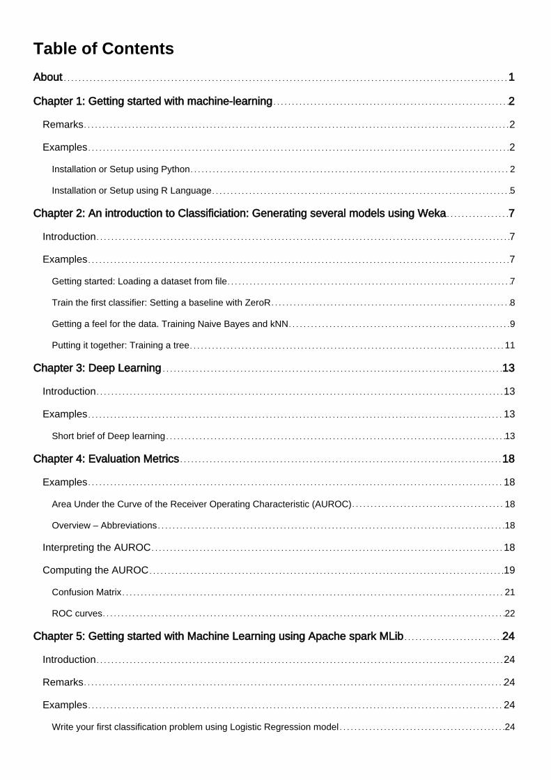
Table of Contents

About 1

Chapter 1: Getting started with machine-learning 2

Remarks 2

Examples 2

Installation or Setup using Python 2

Installation or Setup using R Language 5

Chapter 2: An introduction to Classificiation: Generating several models using Weka 7

Introduction 7

Examples 7

Getting started: Loading a dataset from file 7

Train the first classifier: Setting a baseline with ZeroR 8

Getting a feel for the data. Training Naive Bayes and kNN 9

Putting it together: Training a tree 11

Chapter 3: Deep Learning 13

Introduction 13

Examples 13

Short brief of Deep learning 13

Chapter 4: Evaluation Metrics 18

Examples 18

Area Under the Curve of the Receiver Operating Characteristic (AUROC) 18

Overview – Abbreviations 18

Interpreting the AUROC 18

Computing the AUROC 19

Confusion Matrix 21

ROC curves 22

Chapter 5: Getting started with Machine Learning using Apache spark MLib 24

Introduction 24

Remarks 24

Examples 24

Write your first classification problem using Logistic Regression model 24

Chapter 6: Machine learning and it's classification 28

Examples 28

What is machine learning ? 28

What is supervised learning ? 28

What is unsupervised learning ? 29

Chapter 7: Machine Learning Using Java 30

Examples 30

tools list 30

Chapter 8: Natural Language Processing 33

Introduction 33

Examples 33

Text Matching or Similarity 33

Chapter 9: Neural Networks 34

Examples 34

Getting Started: A Simple ANN with Python 34

Backpropagation - The Heart of Neural Networks 37

1. Weights Initialisation 37

2. Forward Pass 38

3. Backward Pass 38

4. Weights/Parameter Update 38

Activation Functions 39

Sigmoid Function 40

Hyperbolic Tangent Function (tanh) 40

ReLU Function 40

Softmax Function 41

___________________________Where does it fit in? _____________________________ 42

Chapter 10: Perceptron 45

Examples 45

What exactly is a perceptron? 45

An Example: 45

NOTE: 46

Implementing a Perceptron model in C++ 46

What is the bias 53

What is the bias 53

Chapter 11: Scikit Learn 55

Examples 55

A Basic Simple Classification Problem(XOR) using k nearest neighbor algorithm 55

Classification in scikit-learn 55

Chapter 12: Supervised Learning 59

Examples 59

Classification 59

Fruit Classification 59

Introduction to Supervised Learning 60

Linear Regression 61

Chapter 13: SVM 64

Examples 64

Difference between logistic regression and SVM 64

Implementing SVM classifier using Scikit-learn: 65

Chapter 14: Types of learning 66

Examples 66

Supervised Learning 66

Regression 66

Classification 66

Reinforcement Learning 66

Unsupervised Learning 67

Credits 68

About

You can share this PDF with anyone you feel could benefit from it, downloaded the latest version from: machine-learning

It is an unofficial and free machine-learning ebook created for educational purposes. All the content is extracted from Stack Overflow Documentation, which is written by many hardworking individuals at Stack Overflow. It is neither affiliated with Stack Overflow nor official machine-learning.

The content is released under Creative Commons BY-SA, and the list of contributors to each chapter are provided in the credits section at the end of this book. Images may be copyright of their respective owners unless otherwise specified. All trademarks and registered trademarks are the property of their respective company owners.

Use the content presented in this book at your own risk; it is not guaranteed to be correct nor accurate, please send your feedback and corrections to info@zzzprojects.com

https://riptutorial.com/ 1

Chapter 1: Getting started with machine-learning

Remarks

Machine Learning is the science (and art) of programming computers so they can learn from data.

A more formal definition:

It is the field of study that gives computers the ability to learn without being explicitly programmed. Arthur Samuel, 1959

A more engineering-oriented definition:

A computer program is said to learn from experience E with respect to some task T and some performance measure P, if its performance on T, as measured by P, improves with experience   E. Tom Mitchell, 1997

Source: “Hands-On Machine Learning with Scikit-Learn and TensorFlow by Aurélien Géron (O’Reilly). Copyright 2017 Aurélien Géron, 978-1-491-96229-9.”

Machine learning (ML) is a field of computer science which spawned out of research in artificial intelligence. The strength of machine learning over other forms of analytics is in its ability to uncover hidden insights and predict outcomes of future, unseen inputs (generalization). Unlike iterative algorithms where operations are explicitly declared, machine learning algorithms borrow concepts from probability theory to select, evaluate, and improve statistical models.

Examples

Installation or Setup using Python

1) scikit learn

scikit-learn is a Python module for machine learning built on top of SciPy and distributed under the 3-Clause BSD license. It features various classification, regression and clustering algorithms including support vector machines, random forests, gradient boosting, k-means and DBSCAN, and is designed to interoperate with the Python numerical and scientific libraries NumPy and SciPy.

The current stable version of scikit-learn requires:

Python (>= 2.6 or >= 3.3),•NumPy (>= 1.6.1),•SciPy (>= 0.9).•

For most installation pip python package manager can install python and all of its dependencies:

https://riptutorial.com/ 2

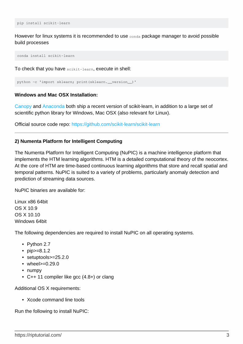
pip install scikit-learn

However for linux systems it is recommended to use conda package manager to avoid possible build processes

conda install scikit-learn

To check that you have scikit-learn, execute in shell:

python -c 'import sklearn; print(sklearn.__version__)'

Windows and Mac OSX Installation:

Canopy and Anaconda both ship a recent version of scikit-learn, in addition to a large set of scientific python library for Windows, Mac OSX (also relevant for Linux).

Official source code repo: https://github.com/scikit-learn/scikit-learn

2) Numenta Platform for Intelligent Computing

The Numenta Platform for Intelligent Computing (NuPIC) is a machine intelligence platform that implements the HTM learning algorithms. HTM is a detailed computational theory of the neocortex. At the core of HTM are time-based continuous learning algorithms that store and recall spatial and temporal patterns. NuPIC is suited to a variety of problems, particularly anomaly detection and prediction of streaming data sources.

NuPIC binaries are available for:

Linux x86 64bit OS X 10.9 OS X 10.10 Windows 64bit

The following dependencies are required to install NuPIC on all operating systems.

Python 2.7•pip>=8.1.2•setuptools>=25.2.0•wheel>=0.29.0•numpy•C++ 11 compiler like gcc (4.8+) or clang•

Additional OS X requirements:

Xcode command line tools•

Run the following to install NuPIC:

https://riptutorial.com/ 3

pip install nupic

Official source code repo: https://github.com/numenta/nupic

3) nilearn

Nilearn is a Python module for fast and easy statistical learning on NeuroImaging data. It leverages the scikit-learn Python toolbox for multivariate statistics with applications such as predictive modelling, classification, decoding, or connectivity analysis.

The required dependencies to use the software are:

Python >= 2.6,•setuptools•Numpy >= 1.6.1•SciPy >= 0.9•Scikit-learn >= 0.14.1•Nibabel >= 1.1.0•

If you are using nilearn plotting functionalities or running the examples, matplotlib >= 1.1.1 is required.

If you want to run the tests, you need nose >= 1.2.1 and coverage >= 3.6.

First make sure you have installed all the dependencies listed above. Then you can install nilearn by running the following command in a command prompt:

pip install -U --user nilearn

Official source code repo: https://github.com/nilearn/nilearn/

4) Using Anaconda

Many scientific Python libraries are readily available in Anaconda. You can get installation files from here. On one hand, using Anaconda, you do not to install and configure many packages, it is BSD licensed, and has trivial installation process, available for Python 3 and Python 2, while, on the other hand, it gives you less flexibility. As an example, some state of the art deep learning python packages might use a different version of numpy then Anaconda installed. However, this downside can be dealt with using another python installation separately(In linux and MAC your default one for example).

Anaconda setup prompts you to installation location selection and also prompts you to PATH addition option. If you add Anaconda to your PATH it is expected that your OS will find Anaconda Python as default. Therefore, modifications and future installations will be available for this Python version only.

To make it clear, after installation of Anaconda and you add it to PATH, using Ubuntu 14.04 via terminal if you type

https://riptutorial.com/ 4

python

Voila, Anaconda Python is your default Python, you can start enjoying using many libraries right away. However, if you want to use your old Python

/usr/bin/python

In long story short, Anaconda is one of the fastest way to start machine learning and data analysis with Python.

Installation or Setup using R Language

Packages are collections of R functions, data, and compiled code in a well-defined format. Public (and private) repositories are used to host collections of R packages. The largest collection of R packages is available from CRAN. Some of the most popular R machine learning packages are the following among others:

1) rpart

Description: Recursive partitioning for classification, regression and survival trees. An implementation of most of the functionality of the 1984 book by Breiman, Friedman, Olshen and Stone.

It can be installed from CRAN using the following code:

install.packages("rpart")

Load the package:

library(rpart)

Official source: https://cran.r-project.org/web/packages/rpart/index.html

2) e1071

Description: Functions for latent class analysis, short time Fourier transform, fuzzy clustering,

https://riptutorial.com/ 5

support vector machines, shortest path computation, bagged clustering, naive Bayes classifier etc.

Installation from CRAN:

install.packages("e1071")

Loading the package:

library(e1071)

Official source: https://cran.r-project.org/web/packages/e1071/index.html

3) randomForest

Description: Classification and regression based on a forest of trees using random inputs.

Installation from CRAN:

install.packages("randomForest")

Loading the package:

library(randomForest)

Official source: https://cran.r-project.org/web/packages/randomForest/index.html

4) caret

Description: Misc functions for training and plotting classification and regression models.

Installation from CRAN:

install.packages("caret")

Loading the package:

library(caret)

Official source: https://cran.r-project.org/web/packages/caret/index.html

Read Getting started with machine-learning online: https://riptutorial.com/machine-learning/topic/1151/getting-started-with-machine-learning

https://riptutorial.com/ 6

Chapter 2: An introduction to Classificiation: Generating several models using Weka

Introduction

This tutorial will show you how to use Weka in JAVA code, load data file, train classifiers and explains some of important concepts behind machine learning.

Weka is a toolkit for machine learning. It includes a library of machine learning and visualisation techniques and features a user friendly GUI.

This tutorial includes examples written in JAVA and includes visuals generated with the GUI. I suggest using the GUI to examine data and JAVA code for structured experiments.

Examples

Getting started: Loading a dataset from file

The Iris flower data set is a widely used data set for demonstration purposes. We will load it, inspect it and slightly modify it for later use.

import java.io.File; import java.net.URL; import weka.core.Instances; import weka.core.converters.ArffSaver; import weka.core.converters.CSVLoader; import weka.filters.Filter; import weka.filters.unsupervised.attribute.RenameAttribute; import weka.classifiers.evaluation.Evaluation; import weka.classifiers.rules.ZeroR; import weka.classifiers.bayes.NaiveBayes; import weka.classifiers.lazy.IBk; import weka.classifiers.trees.J48; import weka.classifiers.meta.AdaBoostM1; public class IrisExperiments { public static void main(String args[]) throws Exception { //First we open stream to a data set as provided on http://archive.ics.uci.edu CSVLoader loader = new CSVLoader(); loader.setSource(new URL("http://archive.ics.uci.edu/ml/machine-learning-databases/iris/iris.data").openStream()); Instances data = loader.getDataSet(); //This file has 149 examples with 5 attributes //In order: // sepal length in cm // sepal width in cm // petal length in cm // petal width in cm // class ( Iris Setosa , Iris Versicolour, Iris Virginica)

https://riptutorial.com/ 7

//Let's briefly inspect the data System.out.println("This file has " + data.numInstances()+" examples."); System.out.println("The first example looks like this: "); for(int i = 0; i < data.instance(0).numAttributes();i++ ){ System.out.println(data.instance(0).attribute(i)); } // NOTE that the last attribute is Nominal // It is convention to have a nominal variable at the last index as target variable // Let's tidy up the data a little bit // Nothing too serious just to show how we can manipulate the data with filters RenameAttribute renamer = new RenameAttribute(); renamer.setOptions(weka.core.Utils.splitOptions("-R last -replace Iris-type")); renamer.setInputFormat(data); data = Filter.useFilter(data, renamer); System.out.println("We changed the name of the target class."); System.out.println("And now it looks like this:"); System.out.println(data.instance(0).attribute(4)); //Now we do this for all the attributes renamer.setOptions(weka.core.Utils.splitOptions("-R 1 -replace sepal-length")); renamer.setInputFormat(data); data = Filter.useFilter(data, renamer); renamer.setOptions(weka.core.Utils.splitOptions("-R 2 -replace sepal-width")); renamer.setInputFormat(data); data = Filter.useFilter(data, renamer); renamer.setOptions(weka.core.Utils.splitOptions("-R 3 -replace petal-length")); renamer.setInputFormat(data); data = Filter.useFilter(data, renamer); renamer.setOptions(weka.core.Utils.splitOptions("-R 4 -replace petal-width")); renamer.setInputFormat(data); data = Filter.useFilter(data, renamer); //Lastly we save our newly created file to disk ArffSaver saver = new ArffSaver(); saver.setInstances(data); saver.setFile(new File("IrisSet.arff")); saver.writeBatch(); } }

Train the first classifier: Setting a baseline with ZeroR

ZeroR is a simple classifier. It doesn't operate per instance instead it operates on general distribution of the classes. It selects the class with the largest a priori probability. It is not a good classifier in the sense that it doesn't use any information in the candidate, but it is often used as a baseline. Note: Other baselines can be used aswel, such as: Industry standard classifiers or handcrafted rules

// First we tell our data that it's class is hidden in the last attribute data.setClassIndex(data.numAttributes() -1); // Then we split the data in to two sets

https://riptutorial.com/ 8

// randomize first because we don't want unequal distributions data.randomize(new java.util.Random(0)); Instances testset = new Instances(data, 0, 50); Instances trainset = new Instances(data, 50, 99); // Now we build a classifier // Train it with the trainset ZeroR classifier1 = new ZeroR(); classifier1.buildClassifier(trainset); // Next we test it against the testset Evaluation Test = new Evaluation(trainset); Test.evaluateModel(classifier1, testset); System.out.println(Test.toSummaryString());

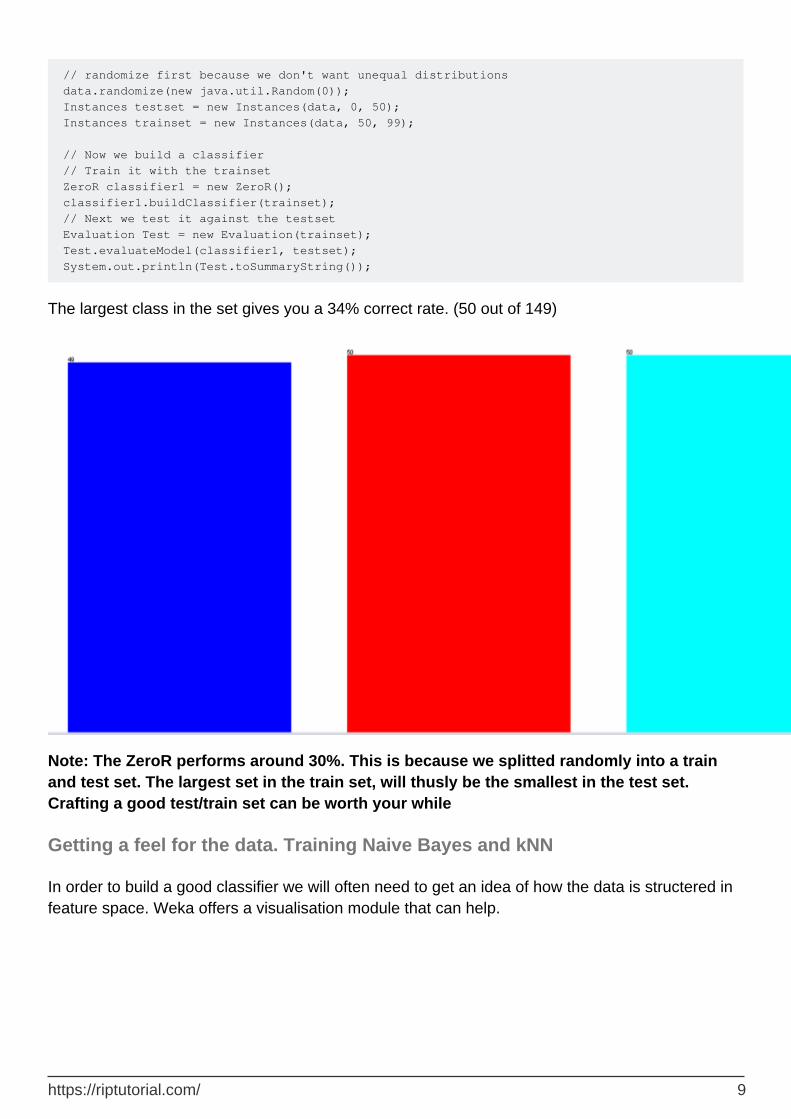
The largest class in the set gives you a 34% correct rate. (50 out of 149)

Note: The ZeroR performs around 30%. This is because we splitted randomly into a train and test set. The largest set in the train set, will thusly be the smallest in the test set. Crafting a good test/train set can be worth your while

Getting a feel for the data. Training Naive Bayes and kNN

In order to build a good classifier we will often need to get an idea of how the data is structered in feature space. Weka offers a visualisation module that can help.

https://riptutorial.com/ 9

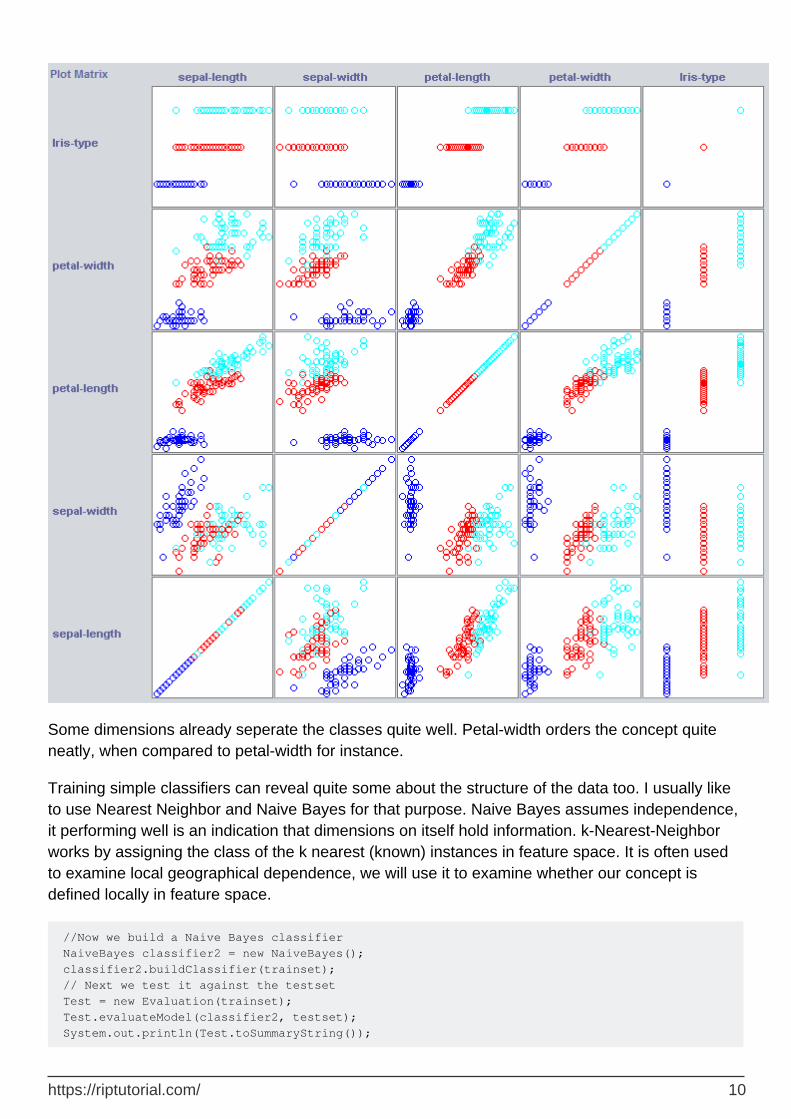
Some dimensions already seperate the classes quite well. Petal-width orders the concept quite neatly, when compared to petal-width for instance.

Training simple classifiers can reveal quite some about the structure of the data too. I usually like to use Nearest Neighbor and Naive Bayes for that purpose. Naive Bayes assumes independence, it performing well is an indication that dimensions on itself hold information. k-Nearest-Neighbor works by assigning the class of the k nearest (known) instances in feature space. It is often used to examine local geographical dependence, we will use it to examine whether our concept is defined locally in feature space.

//Now we build a Naive Bayes classifier NaiveBayes classifier2 = new NaiveBayes(); classifier2.buildClassifier(trainset); // Next we test it against the testset Test = new Evaluation(trainset); Test.evaluateModel(classifier2, testset); System.out.println(Test.toSummaryString());

https://riptutorial.com/ 10

//Now we build a kNN classifier IBk classifier3 = new IBk(); // We tell the classifier to use the first nearest neighbor as example classifier3.setOptions(weka.core.Utils.splitOptions("-K 1")); classifier3.buildClassifier(trainset); // Next we test it against the testset Test = new Evaluation(trainset); Test.evaluateModel(classifier3, testset); System.out.println(Test.toSummaryString());

Naive Bayes performs much better than our freshly established baseline, indcating that independent features hold information (remember petal-width?).

1NN performs well too (in fact a little better in this case), indicating that some of our information is local. The better performance could indicate that some second order effects also hold information (If x and y than class z).

Putting it together: Training a tree

Trees can build models that work on independent features and on second order effects. So they might be good candidates for this domain. Trees are rules that are chaind together, a rule splits instances that arrive at a rule in subgroups, that pass to the rules under the rule.

Tree Learners generate rules, chain them together and stop building trees when they feel the rules get too specific, to avoid overfitting. Overfitting means constructing a model that is too complex for the concept we are looking for. Overfitted models perform well on the train data, but poorly on new data

We use J48, a JAVA implementation of C4.5 a popular algorithm.

//We train a tree using J48 //J48 is a JAVA implementation of the C4.5 algorithm J48 classifier4 = new J48(); //We set it's confidence level to 0.1 //The confidence level tell J48 how specific a rule can be before it gets pruned classifier4.setOptions(weka.core.Utils.splitOptions("-C 0.1")); classifier4.buildClassifier(trainset); // Next we test it against the testset Test = new Evaluation(trainset); Test.evaluateModel(classifier4, testset); System.out.println(Test.toSummaryString()); System.out.print(classifier4.toString()); //We set it's confidence level to 0.5 //Allowing the tree to maintain more complex rules classifier4.setOptions(weka.core.Utils.splitOptions("-C 0.5")); classifier4.buildClassifier(trainset); // Next we test it against the testset Test = new Evaluation(trainset); Test.evaluateModel(classifier4, testset); System.out.println(Test.toSummaryString()); System.out.print(classifier4.toString());

https://riptutorial.com/ 11

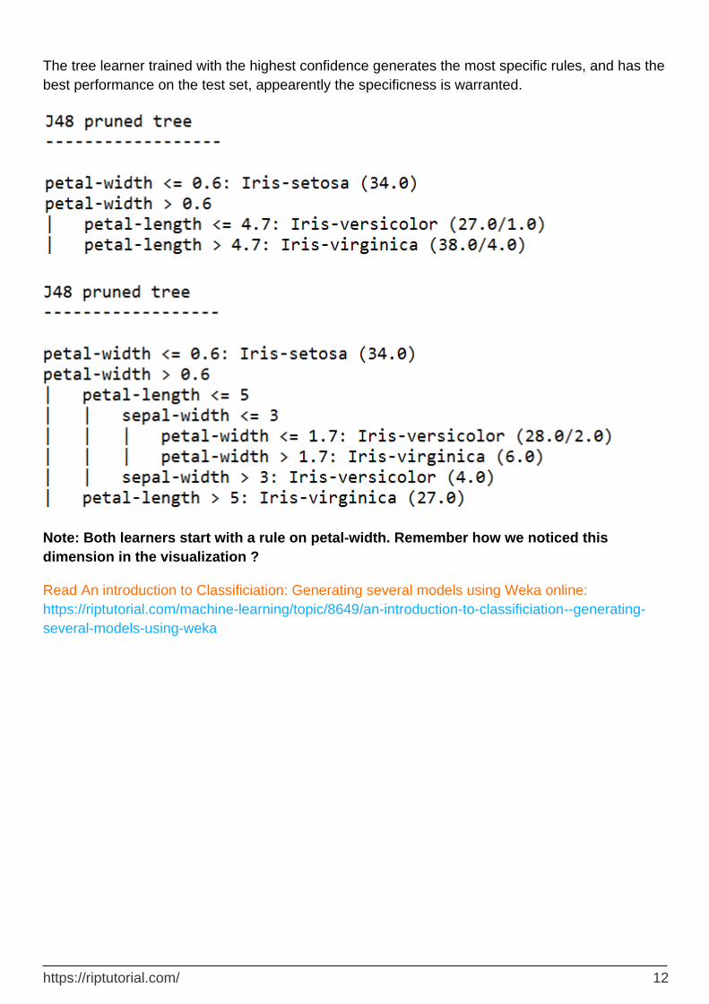
The tree learner trained with the highest confidence generates the most specific rules, and has the best performance on the test set, appearently the specificness is warranted.

Note: Both learners start with a rule on petal-width. Remember how we noticed this dimension in the visualization ?

Read An introduction to Classificiation: Generating several models using Weka online: https://riptutorial.com/machine-learning/topic/8649/an-introduction-to-classificiation--generating-several-models-using-weka

https://riptutorial.com/ 12

Chapter 3: Deep Learning

Introduction

Deep Learning is a sub-field of machine learning where multi-layer artificial neural networks are used for learning purpose. Deep Learning has found lots of great implementations, e.g. Speech Recognition, Subtitles on Youtube, Amazon recommendation, and so on. For additional information there is a dedicated topic to deep-learning.

Examples

Short brief of Deep learning

To train a neural network, firstly we need to design a good and efficient idea. There are three types of learning tasks.

Supervised Learning•Reinforcement Learning•Unsupervised Learning•

In this present time, unsupervised learning is very popular.Unsupervised Learning is a deep learning task of inferring a function to describe hidden structure from "unlabeled" data (a classification or categorization is not included in the observations).

Since the examples given to the learner are unlabeled, there is no evaluation of the accuracy of the structure that is output by the relevant algorithm—which is one way of distinguishing unsupervised learning from Supervised Learning and Reinforcement Learning.

There are three types of Unsupervised learning.

Restricted Boltzmann Machines•Sparse Coding Model•Autoencoders I will describe in detail of autoencoder.•

The aim of an autoencoder is to learn a representation (encoding) for a set of data, typically for the purpose of dimensionality reduction.

The simplest form of an autoencoder is a feedforward, having an input layer, an output layer and one or more hidden layers connecting them. But with the output layer having the same number of nodes as the input layer, and with the purpose of reconstructing its own inputs and that's why it is called unsupervised learning.

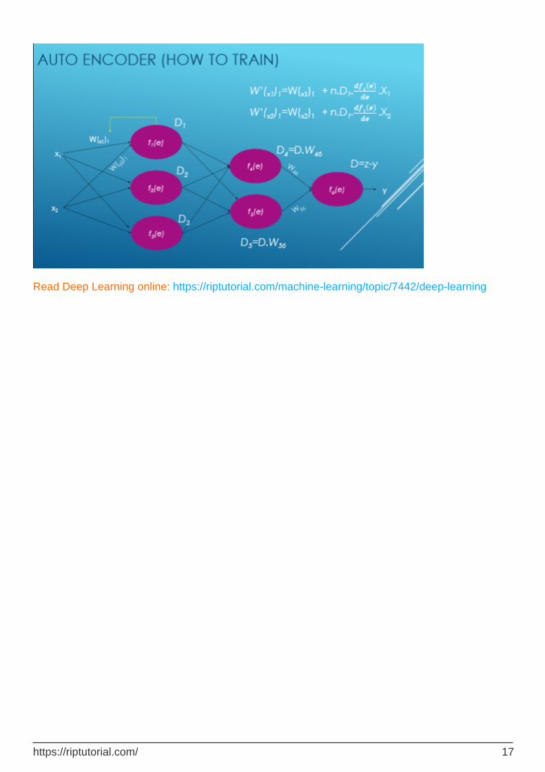
Now I will try to give an example of training neural network.

https://riptutorial.com/ 13

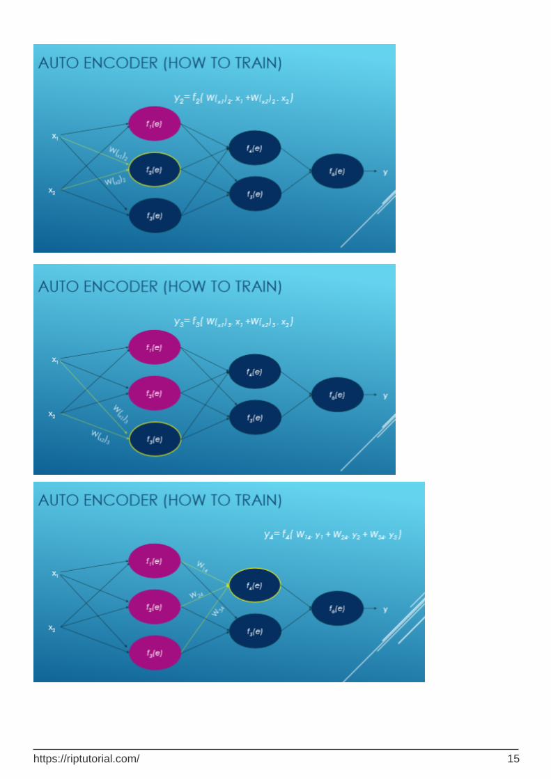
Here Xi is input, W is weight, f(e) is activation function and y is output.

Now we see step by step flow of training neural network based on autoencoder.

We calculate every activation function's value with this equation: y=WiXi. First of all, we randomly pick numbers for weights and then try to adjust that weights.

https://riptutorial.com/ 14

https://riptutorial.com/ 15

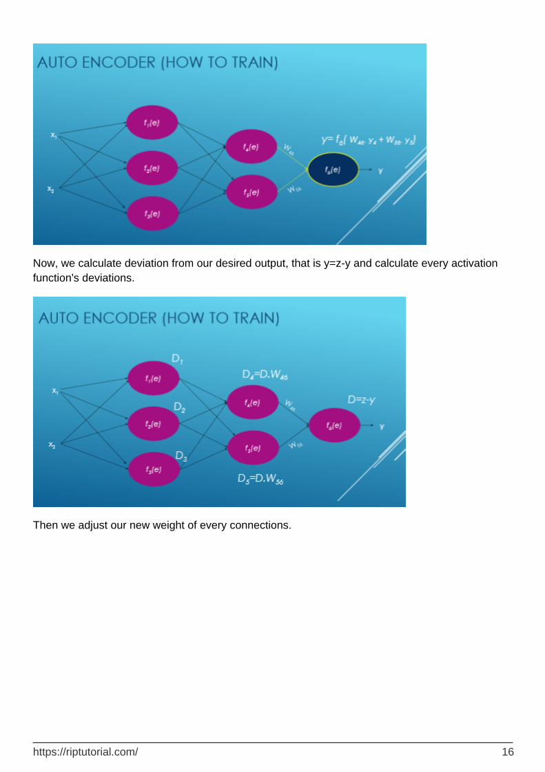
Now, we calculate deviation from our desired output, that is y=z-y and calculate every activation function's deviations.

Then we adjust our new weight of every connections.

https://riptutorial.com/ 16

Read Deep Learning online: https://riptutorial.com/machine-learning/topic/7442/deep-learning

https://riptutorial.com/ 17

Chapter 4: Evaluation Metrics

Examples

Area Under the Curve of the Receiver Operating Characteristic (AUROC)

The AUROC is one of the most commonly used metric to evaluate a classifier's performances. This section explains how to compute it.

AUC (Area Under the Curve) is used most of the time to mean AUROC, which is a bad practice as AUC is ambiguous (could be any curve) while AUROC is not.

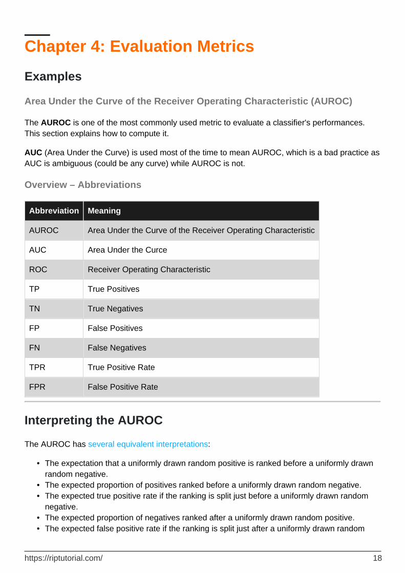
Overview – Abbreviations

Abbreviation Meaning

AUROC Area Under the Curve of the Receiver Operating Characteristic

AUC Area Under the Curce

ROC Receiver Operating Characteristic

TP True Positives

TN True Negatives

FP False Positives

FN False Negatives

TPR True Positive Rate

FPR False Positive Rate

Interpreting the AUROC

The AUROC has several equivalent interpretations:

The expectation that a uniformly drawn random positive is ranked before a uniformly drawn random negative.

•

The expected proportion of positives ranked before a uniformly drawn random negative.•The expected true positive rate if the ranking is split just before a uniformly drawn random negative.

•

The expected proportion of negatives ranked after a uniformly drawn random positive.•The expected false positive rate if the ranking is split just after a uniformly drawn random •

https://riptutorial.com/ 18

positive.

Computing the AUROC

Assume we have a probabilistic, binary classifier such as logistic regression.

Before presenting the ROC curve (= Receiver Operating Characteristic curve), the concept of confusion matrix must be understood. When we make a binary prediction, there can be 4 types of outcomes:

We predict 0 while the class is actually 0: this is called a True Negative, i.e. we correctly predict that the class is negative (0). For example, an antivirus did not detect a harmless file as a virus.

•

We predict 0 while the class is actually 1: this is called a False Negative, i.e. we incorrectly predict that the class is negative (0). For example, an antivirus failed to detect a virus.

•

We predict 1 while the class is actually 0: this is called a False Positive, i.e. we incorrectly predict that the class is positive (1). For example, an antivirus considered a harmless file to be a virus.

•

We predict 1 while the class is actually 1: this is called a True Positive, i.e. we correctly predict that the class is positive (1). For example, an antivirus rightfully detected a virus.

•

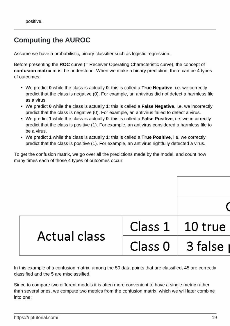
To get the confusion matrix, we go over all the predictions made by the model, and count how many times each of those 4 types of outcomes occur:

In this example of a confusion matrix, among the 50 data points that are classified, 45 are correctly classified and the 5 are misclassified.

Since to compare two different models it is often more convenient to have a single metric rather than several ones, we compute two metrics from the confusion matrix, which we will later combine into one:

https://riptutorial.com/ 19

True positive rate (TPR), aka. sensitivity, hit rate, and recall, which is defined as

. Intuitively this metric corresponds to the proportion of positive data points that are correctly considered as positive, with respect to all positive data points. In other words, the higher TPR, the fewer positive data points we will miss.

•

False positive rate (FPR), aka. fall-out, which is defined as

. Intuitively this metric corresponds to the proportion of negative data points that are mistakenly considered as positive, with respect to all negative data points. In other words, the higher FPR, the more negative data points we will missclassified.

•

To combine the FPR and the TPR into one single metric, we first compute the two former metrics

with many different threshold (for example ) for the logistic regression, then plot them on a single graph, with the FPR values on the abscissa and the TPR values on the ordinate. The resulting curve is called ROC curve, and the metric we consider is the AUC of this curve, which we call AUROC.

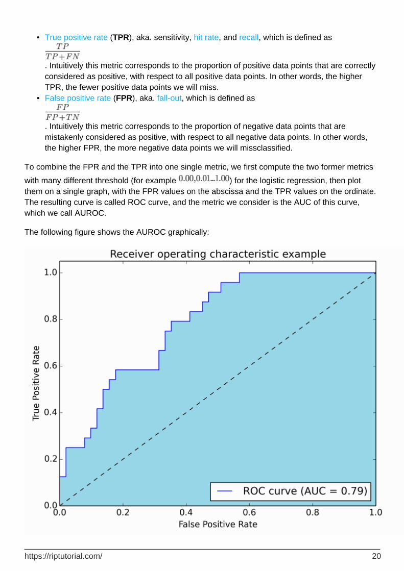
The following figure shows the AUROC graphically:

https://riptutorial.com/ 20

In this figure, the blue area corresponds to the Area Under the curve of the Receiver Operating Characteristic (AUROC). The dashed line in the diagonal we present the ROC curve of a random predictor: it has an AUROC of 0.5. The random predictor is commonly used as a baseline to see whether the model is useful.

Confusion Matrix

A confusion matrix can be used to evaluate a classifier, based on a set of test data for which the true values are known. It is a simple tool, that helps to give a good visual overview of the performance of the algorithm being used.

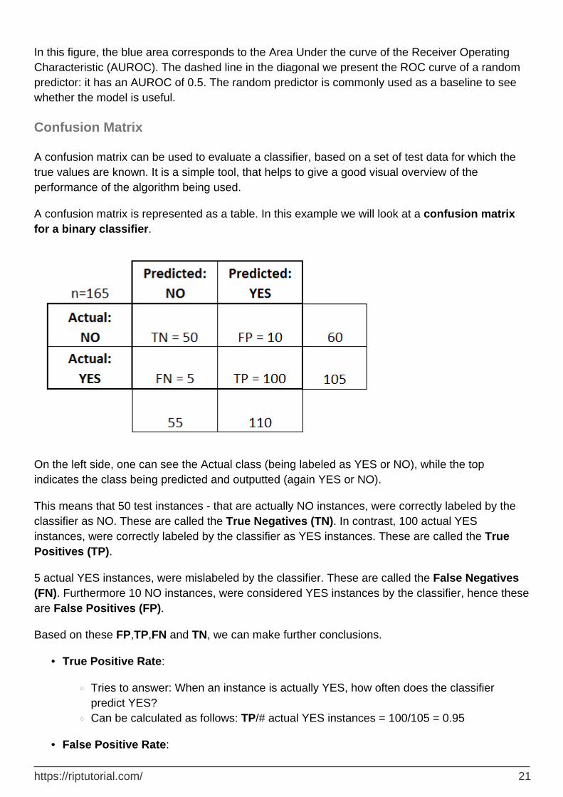
A confusion matrix is represented as a table. In this example we will look at a confusion matrix for a binary classifier.

On the left side, one can see the Actual class (being labeled as YES or NO), while the top indicates the class being predicted and outputted (again YES or NO).

This means that 50 test instances - that are actually NO instances, were correctly labeled by the classifier as NO. These are called the True Negatives (TN). In contrast, 100 actual YES instances, were correctly labeled by the classifier as YES instances. These are called the True Positives (TP).

5 actual YES instances, were mislabeled by the classifier. These are called the False Negatives (FN). Furthermore 10 NO instances, were considered YES instances by the classifier, hence these are False Positives (FP).

Based on these FP,TP,FN and TN, we can make further conclusions.

True Positive Rate:

Tries to answer: When an instance is actually YES, how often does the classifier predict YES?

○

Can be calculated as follows: TP/# actual YES instances = 100/105 = 0.95○

•

False Positive Rate:•

https://riptutorial.com/ 21

Tries to answer: When an instance is actually NO, how often does the classifier predict YES?

○

Can be calculated as follows: FP/# actual NO instances = 10/60 = 0.17○

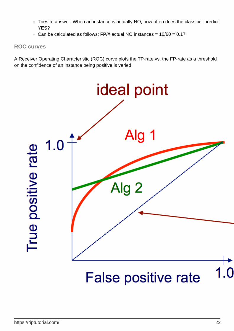
ROC curves

A Receiver Operating Characteristic (ROC) curve plots the TP-rate vs. the FP-rate as a threshold on the confidence of an instance being positive is varied

https://riptutorial.com/ 22

Algorithm for creating an ROC curve

sort test-set predictions according to confidence that each instance is positive1.

step through sorted list from high to low confidence

i. locate a threshold between instances with opposite classes (keeping instances with the same confidence value on the same side of threshold)

ii. compute TPR, FPR for instances above threshold

iii. output (FPR, TPR) coordinate

2.

Read Evaluation Metrics online: https://riptutorial.com/machine-learning/topic/4132/evaluation-metrics

https://riptutorial.com/ 23

Chapter 5: Getting started with Machine Learning using Apache spark MLib

Introduction

Apache spark MLib provides (JAVA, R, PYTHON, SCALA) 1.) Various Machine learning algorithms on regression, classification, clustering, collaborative filtering which are mostly used approaches in Machine learning. 2.) It supports feature extraction, transformation etc. 3.) It allows data practitioners to solve their machine learning problems (as well as graph computation, streaming, and real-time interactive query processing) interactively and at much greater scale.

Remarks

Please refer below given to know more about spark MLib

http://spark.apache.org/docs/latest/ml-guide.html1. https://mapr.com/ebooks/spark/2.

Examples

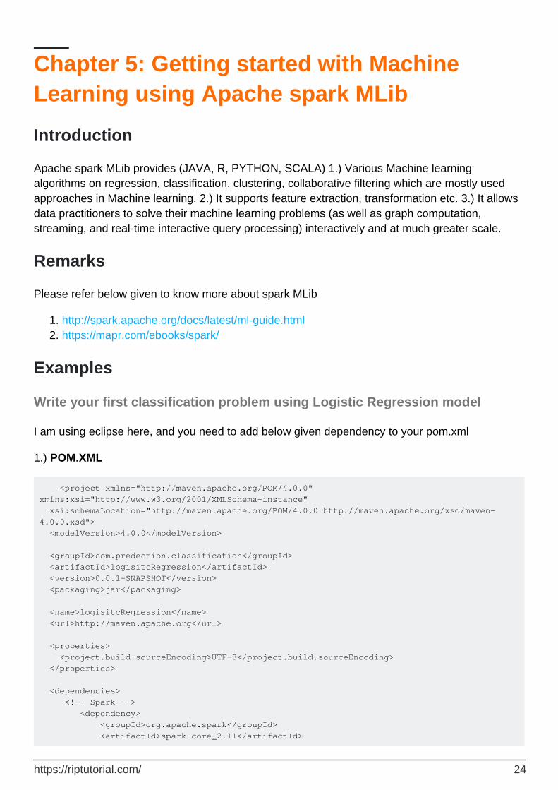
Write your first classification problem using Logistic Regression model

I am using eclipse here, and you need to add below given dependency to your pom.xml

1.) POM.XML

<project xmlns="http://maven.apache.org/POM/4.0.0" xmlns:xsi="http://www.w3.org/2001/XMLSchema-instance" xsi:schemaLocation="http://maven.apache.org/POM/4.0.0 http://maven.apache.org/xsd/maven-4.0.0.xsd"> <modelVersion>4.0.0</modelVersion> <groupId>com.predection.classification</groupId> <artifactId>logisitcRegression</artifactId> <version>0.0.1-SNAPSHOT</version> <packaging>jar</packaging> <name>logisitcRegression</name> <url>http://maven.apache.org</url> <properties> <project.build.sourceEncoding>UTF-8</project.build.sourceEncoding> </properties> <dependencies> <!-- Spark --> <dependency> <groupId>org.apache.spark</groupId> <artifactId>spark-core_2.11</artifactId>

https://riptutorial.com/ 24

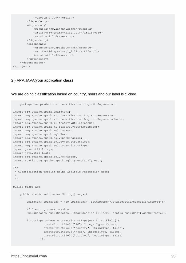
<version>2.1.0</version> </dependency> <dependency> <groupId>org.apache.spark</groupId> <artifactId>spark-mllib_2.10</artifactId> <version>2.1.0</version> </dependency> <dependency> <groupId>org.apache.spark</groupId> <artifactId>spark-sql_2.11</artifactId> <version>2.1.0</version> </dependency> </dependencies> </project>

2.) APP.JAVA(your application class)

We are doing classification based on country, hours and our label is clicked.

package com.predection.classification.logisitcRegression; import org.apache.spark.SparkConf; import org.apache.spark.ml.classification.LogisticRegression; import org.apache.spark.ml.classification.LogisticRegressionModel; import org.apache.spark.ml.feature.StringIndexer; import org.apache.spark.ml.feature.VectorAssembler; import org.apache.spark.sql.Dataset; import org.apache.spark.sql.Row; import org.apache.spark.sql.SparkSession; import org.apache.spark.sql.types.StructField; import org.apache.spark.sql.types.StructType; import java.util.Arrays; import java.util.List; import org.apache.spark.sql.RowFactory; import static org.apache.spark.sql.types.DataTypes.*; /** * Classification problem using Logistic Regression Model * */ public class App { public static void main( String[] args ) { SparkConf sparkConf = new SparkConf().setAppName("JavaLogisticRegressionExample"); // Creating spark session SparkSession sparkSession = SparkSession.builder().config(sparkConf).getOrCreate(); StructType schema = createStructType(new StructField[]{ createStructField("id", IntegerType, false), createStructField("country", StringType, false), createStructField("hour", IntegerType, false), createStructField("clicked", DoubleType, false) });

https://riptutorial.com/ 25

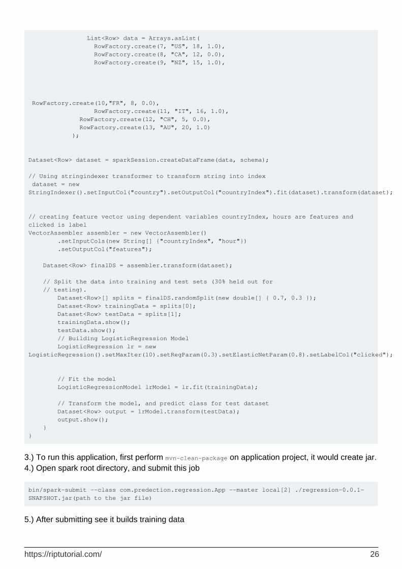
List<Row> data = Arrays.asList( RowFactory.create(7, "US", 18, 1.0), RowFactory.create(8, "CA", 12, 0.0), RowFactory.create(9, "NZ", 15, 1.0), RowFactory.create(10,"FR", 8, 0.0), RowFactory.create(11, "IT", 16, 1.0), RowFactory.create(12, "CH", 5, 0.0), RowFactory.create(13, "AU", 20, 1.0) ); Dataset<Row> dataset = sparkSession.createDataFrame(data, schema); // Using stringindexer transformer to transform string into index dataset = new StringIndexer().setInputCol("country").setOutputCol("countryIndex").fit(dataset).transform(dataset); // creating feature vector using dependent variables countryIndex, hours are features and clicked is label VectorAssembler assembler = new VectorAssembler() .setInputCols(new String[] {"countryIndex", "hour"}) .setOutputCol("features"); Dataset<Row> finalDS = assembler.transform(dataset); // Split the data into training and test sets (30% held out for // testing). Dataset<Row>[] splits = finalDS.randomSplit(new double[] { 0.7, 0.3 }); Dataset<Row> trainingData = splits[0]; Dataset<Row> testData = splits[1]; trainingData.show(); testData.show(); // Building LogisticRegression Model LogisticRegression lr = new LogisticRegression().setMaxIter(10).setRegParam(0.3).setElasticNetParam(0.8).setLabelCol("clicked"); // Fit the model LogisticRegressionModel lrModel = lr.fit(trainingData); // Transform the model, and predict class for test dataset Dataset<Row> output = lrModel.transform(testData); output.show(); } }

3.) To run this application, first perform mvn-clean-package on application project, it would create jar. 4.) Open spark root directory, and submit this job

bin/spark-submit --class com.predection.regression.App --master local[2] ./regression-0.0.1-SNAPSHOT.jar(path to the jar file)

5.) After submitting see it builds training data

https://riptutorial.com/ 26

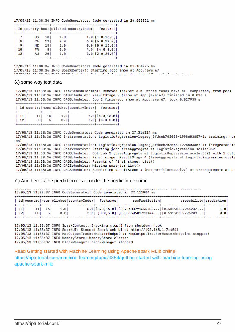
6.) same way test data

7.) And here is the prediction result under the prediction column

Read Getting started with Machine Learning using Apache spark MLib online: https://riptutorial.com/machine-learning/topic/9854/getting-started-with-machine-learning-using-apache-spark-mlib

https://riptutorial.com/ 27

Chapter 6: Machine learning and it's classification

Examples

What is machine learning ?

Two definitions of Machine Learning are offered. Arthur Samuel described it as:

the field of study that gives computers the ability to learn without being explicitly programmed.

This is an older, informal definition.

Tom Mitchell provides a more modern definition:

A computer program is said to learn from experience E with respect to some class of tasks T and performance measure P, if its performance at tasks in T, as measured by P, improves with experience E.

Example: playing checkers.

E = the experience of playing many games of checkers

T = the task of playing checkers.

P = the probability that the program will win the next game.

In general, any machine learning problem can be assigned to one of two broad classifications:

Supervised learning1. Unsupervised learning.2.

What is supervised learning ?

Supervised learning is a type of machine learning algorithm that uses a known data-set (called the training data-set) to make predictions.

Category of supervised learning:

Regression: In a regression problem, we are trying to predict results within a continuous output, meaning that we are trying to map input variables to some continuous function.

1.

Classification: In a classification problem, we are instead trying to predict results in a discrete output. In other words, we are trying to map input variables into discrete categories.

2.

Example 1:

https://riptutorial.com/ 28

Given data about the size of houses on the real estate market, try to predict their price. Price as a function of size is a continuous output, so this is a regression problem.

Example 2:

(a) Regression - For continuous-response values. For example given a picture of a person, we have to predict their age on the basis of the given picture

(b) Classification - for categorical response values, where the data can be separated into specific “classes”. For example given a patient with a tumor, we have to predict whether the tumor is malignant or benign.

What is unsupervised learning ?

Unsupervised learning allows us to approach problems with little or no idea what our results should look like. We can derive structure from data where we don't necessarily know the effect of the variables.

Example:

Clustering: Is used for exploratory data analysis to find hidden patterns or grouping in data. Take a collection of 1,000,000 different genes, and find a way to automatically group these genes into groups that are somehow similar or related by different variables, such as lifespan, location, roles, and so on.

Read Machine learning and it's classification online: https://riptutorial.com/machine-learning/topic/9986/machine-learning-and-it-s-classification

https://riptutorial.com/ 29

Chapter 7: Machine Learning Using Java

Examples

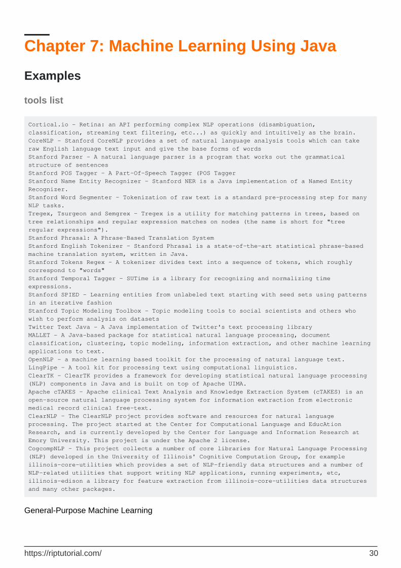
tools list

Cortical.io - Retina: an API performing complex NLP operations (disambiguation, classification, streaming text filtering, etc...) as quickly and intuitively as the brain. CoreNLP - Stanford CoreNLP provides a set of natural language analysis tools which can take raw English language text input and give the base forms of words Stanford Parser - A natural language parser is a program that works out the grammatical structure of sentences Stanford POS Tagger - A Part-Of-Speech Tagger (POS Tagger Stanford Name Entity Recognizer - Stanford NER is a Java implementation of a Named Entity Recognizer. Stanford Word Segmenter - Tokenization of raw text is a standard pre-processing step for many NLP tasks. Tregex, Tsurgeon and Semgrex - Tregex is a utility for matching patterns in trees, based on tree relationships and regular expression matches on nodes (the name is short for "tree regular expressions"). Stanford Phrasal: A Phrase-Based Translation System Stanford English Tokenizer - Stanford Phrasal is a state-of-the-art statistical phrase-based machine translation system, written in Java. Stanford Tokens Regex - A tokenizer divides text into a sequence of tokens, which roughly correspond to "words" Stanford Temporal Tagger - SUTime is a library for recognizing and normalizing time expressions. Stanford SPIED - Learning entities from unlabeled text starting with seed sets using patterns in an iterative fashion Stanford Topic Modeling Toolbox - Topic modeling tools to social scientists and others who wish to perform analysis on datasets Twitter Text Java - A Java implementation of Twitter's text processing library MALLET - A Java-based package for statistical natural language processing, document classification, clustering, topic modeling, information extraction, and other machine learning applications to text. OpenNLP - a machine learning based toolkit for the processing of natural language text. LingPipe - A tool kit for processing text using computational linguistics. ClearTK - ClearTK provides a framework for developing statistical natural language processing (NLP) components in Java and is built on top of Apache UIMA. Apache cTAKES - Apache clinical Text Analysis and Knowledge Extraction System (cTAKES) is an open-source natural language processing system for information extraction from electronic medical record clinical free-text. ClearNLP - The ClearNLP project provides software and resources for natural language processing. The project started at the Center for Computational Language and EducAtion Research, and is currently developed by the Center for Language and Information Research at Emory University. This project is under the Apache 2 license. CogcompNLP - This project collects a number of core libraries for Natural Language Processing (NLP) developed in the University of Illinois' Cognitive Computation Group, for example illinois-core-utilities which provides a set of NLP-friendly data structures and a number of NLP-related utilities that support writing NLP applications, running experiments, etc, illinois-edison a library for feature extraction from illinois-core-utilities data structures and many other packages.

General-Purpose Machine Learning

https://riptutorial.com/ 30

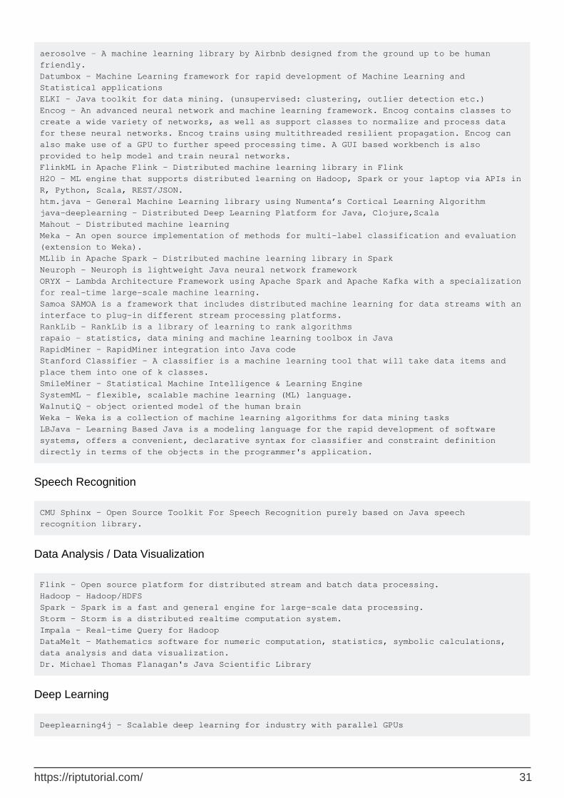
aerosolve - A machine learning library by Airbnb designed from the ground up to be human friendly. Datumbox - Machine Learning framework for rapid development of Machine Learning and Statistical applications ELKI - Java toolkit for data mining. (unsupervised: clustering, outlier detection etc.) Encog - An advanced neural network and machine learning framework. Encog contains classes to create a wide variety of networks, as well as support classes to normalize and process data for these neural networks. Encog trains using multithreaded resilient propagation. Encog can also make use of a GPU to further speed processing time. A GUI based workbench is also provided to help model and train neural networks. FlinkML in Apache Flink - Distributed machine learning library in Flink H2O - ML engine that supports distributed learning on Hadoop, Spark or your laptop via APIs in R, Python, Scala, REST/JSON. htm.java - General Machine Learning library using Numenta’s Cortical Learning Algorithm java-deeplearning - Distributed Deep Learning Platform for Java, Clojure,Scala Mahout - Distributed machine learning Meka - An open source implementation of methods for multi-label classification and evaluation (extension to Weka). MLlib in Apache Spark - Distributed machine learning library in Spark Neuroph - Neuroph is lightweight Java neural network framework ORYX - Lambda Architecture Framework using Apache Spark and Apache Kafka with a specialization for real-time large-scale machine learning. Samoa SAMOA is a framework that includes distributed machine learning for data streams with an interface to plug-in different stream processing platforms. RankLib - RankLib is a library of learning to rank algorithms rapaio - statistics, data mining and machine learning toolbox in Java RapidMiner - RapidMiner integration into Java code Stanford Classifier - A classifier is a machine learning tool that will take data items and place them into one of k classes. SmileMiner - Statistical Machine Intelligence & Learning Engine SystemML - flexible, scalable machine learning (ML) language. WalnutiQ - object oriented model of the human brain Weka - Weka is a collection of machine learning algorithms for data mining tasks LBJava - Learning Based Java is a modeling language for the rapid development of software systems, offers a convenient, declarative syntax for classifier and constraint definition directly in terms of the objects in the programmer's application.

Speech Recognition

CMU Sphinx - Open Source Toolkit For Speech Recognition purely based on Java speech recognition library.

Data Analysis / Data Visualization

Flink - Open source platform for distributed stream and batch data processing. Hadoop - Hadoop/HDFS Spark - Spark is a fast and general engine for large-scale data processing. Storm - Storm is a distributed realtime computation system. Impala - Real-time Query for Hadoop DataMelt - Mathematics software for numeric computation, statistics, symbolic calculations, data analysis and data visualization. Dr. Michael Thomas Flanagan's Java Scientific Library

Deep Learning

Deeplearning4j - Scalable deep learning for industry with parallel GPUs

https://riptutorial.com/ 31

Read Machine Learning Using Java online: https://riptutorial.com/machine-learning/topic/6175/machine-learning-using-java

https://riptutorial.com/ 32

Chapter 8: Natural Language Processing

Introduction

NLP is a way for computers to analyze, understand, and derive meaning from human language in a smart and useful way. By utilizing NLP, developers can organize and structure knowledge to perform tasks such as automatic summarization, translation, named entity recognition, relationship extraction, sentiment analysis, speech recognition, and topic segmentation.

Examples

Text Matching or Similarity

One of the important areas of NLP is the matching of text objects to find similarities. Important applications of text matching includes automatic spelling correction, data de-duplication and genome analysis etc. A number of text matching techniques are available depending upon the requirement. So lets have;Levenshtein Distance

The Levenshtein distance between two strings is defined as the minimum number of edits needed to transform one string into the other, with the allowable edit operations being insertion, deletion, or substitution of a single character.

Following is the implementation for efficient memory computations.

def levenshtein(s1,s2): if len(s1) > len(s2): s1,s2 = s2,s1 distances = range(len(s1) + 1) for index2,char2 in enumerate(s2): newDistances = [index2+1] for index1,char1 in enumerate(s1): if char1 == char2: newDistances.append(distances[index1]) else: newDistances.append(1 + min((distances[index1], distances[index1+1], newDistances[-1]))) distances = newDistances return distances[-1] print(levenshtein("analyze","analyse"))

Read Natural Language Processing online: https://riptutorial.com/machine-learning/topic/10734/natural-language-processing

https://riptutorial.com/ 33

Chapter 9: Neural Networks

Examples

Getting Started: A Simple ANN with Python

The code listing below attempts to classify handwritten digits from the MNIST dataset. The digits look like this:

The code will preprocess these digits, converting each image into a 2D array of 0s and 1s, and then use this data to train a neural network with upto 97% accuracy (50 epochs).

""" Deep Neural Net (Name: Classic Feedforward) """ import numpy as np import pickle, json import sklearn.datasets import random import time import os def sigmoid(z): return 1.0 / (1.0 + np.exp(-z)) def sigmoid_prime(z): return sigmoid(z) * (1 - sigmoid(z)) def relU(z): return np.maximum(z, 0, z) def relU_prime(z): return z * (z <= 0) def tanh(z): return np.tanh(z)

https://riptutorial.com/ 34

def tanh_prime(z): return 1 - (tanh(z) ** 2) def transform_target(y): t = np.zeros((10, 1)) t[int(y)] = 1.0 return t """--------------------------------------------------------------------------------""" class NeuralNet: def __init__(self, layers, learning_rate=0.05, reg_lambda=0.01): self.num_layers = len(layers) self.layers = layers self.biases = [np.zeros((y, 1)) for y in layers[1:]] self.weights = [np.random.normal(loc=0.0, scale=0.1, size=(y, x)) for x, y in zip(layers[:-1], layers[1:])] self.learning_rate = learning_rate self.reg_lambda = reg_lambda self.nonlinearity = relU self.nonlinearity_prime = relU_prime def __feedforward(self, x): """ Returns softmax probabilities for the output layer """ for w, b in zip(self.weights, self.biases): x = self.nonlinearity(np.dot(w, np.reshape(x, (len(x), 1))) + b) return np.exp(x) / np.sum(np.exp(x)) def __backpropagation(self, x, y): """ :param x: input :param y: target """ weight_gradients = [np.zeros(w.shape) for w in self.weights] bias_gradients = [np.zeros(b.shape) for b in self.biases] # forward pass activation = x hidden_activations = [np.reshape(x, (len(x), 1))] z_list = [] for w, b in zip(self.weights, self.biases): z = np.dot(w, np.reshape(activation, (len(activation), 1))) + b z_list.append(z) activation = self.nonlinearity(z) hidden_activations.append(activation) t = hidden_activations[-1] hidden_activations[-1] = np.exp(t) / np.sum(np.exp(t)) # backward pass delta = (hidden_activations[-1] - y) * (z_list[-1] > 0) weight_gradients[-1] = np.dot(delta, hidden_activations[-2].T) bias_gradients[-1] = delta for l in range(2, self.num_layers): z = z_list[-l] delta = np.dot(self.weights[-l + 1].T, delta) * (z > 0) weight_gradients[-l] = np.dot(delta, hidden_activations[-l - 1].T)

https://riptutorial.com/ 35

bias_gradients[-l] = delta return (weight_gradients, bias_gradients) def __update_params(self, weight_gradients, bias_gradients): for i in xrange(len(self.weights)): self.weights[i] += -self.learning_rate * weight_gradients[i] self.biases[i] += -self.learning_rate * bias_gradients[i] def train(self, training_data, validation_data=None, epochs=10): bias_gradients = None for i in xrange(epochs): random.shuffle(training_data) inputs = [data[0] for data in training_data] targets = [data[1] for data in training_data] for j in xrange(len(inputs)): (weight_gradients, bias_gradients) = self.__backpropagation(inputs[j], targets[j]) self.__update_params(weight_gradients, bias_gradients) if validation_data: random.shuffle(validation_data) inputs = [data[0] for data in validation_data] targets = [data[1] for data in validation_data] for j in xrange(len(inputs)): (weight_gradients, bias_gradients) = self.__backpropagation(inputs[j], targets[j]) self.__update_params(weight_gradients, bias_gradients) print("{} epoch(s) done".format(i + 1)) print("Training done.") def test(self, test_data): test_results = [(np.argmax(self.__feedforward(x[0])), np.argmax(x[1])) for x in test_data] return float(sum([int(x == y) for (x, y) in test_results])) / len(test_data) * 100 def dump(self, file): pickle.dump(self, open(file, "wb")) """--------------------------------------------------------------------------------""" if __name__ == "__main__": total = 5000 training = int(total * 0.7) val = int(total * 0.15) test = int(total * 0.15) mnist = sklearn.datasets.fetch_mldata('MNIST original', data_home='./data') data = zip(mnist.data, mnist.target) random.shuffle(data) data = data[:total] data = [(x[0].astype(bool).astype(int), transform_target(x[1])) for x in data] train_data = data[:training] val_data = data[training:training+val] test_data = data[training+val:]

https://riptutorial.com/ 36

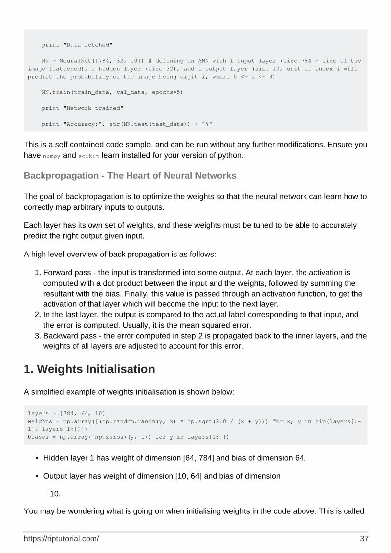
print "Data fetched" NN = NeuralNet([784, 32, 10]) # defining an ANN with 1 input layer (size 784 = size of the image flattened), 1 hidden layer (size 32), and 1 output layer (size 10, unit at index i will predict the probability of the image being digit i, where 0 <= i <= 9) NN.train(train_data, val_data, epochs=5) print "Network trained" print "Accuracy:", str(NN.test(test_data)) + "%"

This is a self contained code sample, and can be run without any further modifications. Ensure you have numpy and scikit learn installed for your version of python.

Backpropagation - The Heart of Neural Networks

The goal of backpropagation is to optimize the weights so that the neural network can learn how to correctly map arbitrary inputs to outputs.

Each layer has its own set of weights, and these weights must be tuned to be able to accurately predict the right output given input.

A high level overview of back propagation is as follows:

Forward pass - the input is transformed into some output. At each layer, the activation is computed with a dot product between the input and the weights, followed by summing the resultant with the bias. Finally, this value is passed through an activation function, to get the activation of that layer which will become the input to the next layer.

1.

In the last layer, the output is compared to the actual label corresponding to that input, and the error is computed. Usually, it is the mean squared error.

2.

Backward pass - the error computed in step 2 is propagated back to the inner layers, and the weights of all layers are adjusted to account for this error.

3.

1. Weights Initialisation

A simplified example of weights initialisation is shown below:

layers = [784, 64, 10] weights = np.array([(np.random.randn(y, x) * np.sqrt(2.0 / (x + y))) for x, y in zip(layers[:-1], layers[1:])]) biases = np.array([np.zeros((y, 1)) for y in layers[1:]])

Hidden layer 1 has weight of dimension [64, 784] and bias of dimension 64.•

Output layer has weight of dimension [10, 64] and bias of dimension

10.

•

You may be wondering what is going on when initialising weights in the code above. This is called

https://riptutorial.com/ 37

Xavier initialisation, and it is a step better than randomly initialising your weight matrices. Yes, initialisation does matter. Based on your initialisation, you might be able to find a better local minima during gradient descent (back propagation is a glorified version of gradient descent).

2. Forward Pass

activation = x hidden_activations = [np.reshape(x, (len(x), 1))] z_list = [] for w, b in zip(self.weights, self.biases): z = np.dot(w, np.reshape(activation, (len(activation), 1))) + b z_list.append(z) activation = relu(z) hidden_activations.append(activation) t = hidden_activations[-1] hidden_activations[-1] = np.exp(t) / np.sum(np.exp(t))

This code carries out the transformation described above. hidden_activations[-1] contains softmax probabilities - predictions of all classes, the sum of which is 1. If we are predicting digits, then output will be a vector of probabilities of dimension 10, the sum of which is 1.

3. Backward Pass

weight_gradients = [np.zeros(w.shape) for w in self.weights] bias_gradients = [np.zeros(b.shape) for b in self.biases] delta = (hidden_activations[-1] - y) * (z_list[-1] > 0) # relu derivative weight_gradients[-1] = np.dot(delta, hidden_activations[-2].T) bias_gradients[-1] = delta for l in range(2, self.num_layers): z = z_list[-l] delta = np.dot(self.weights[-l + 1].T, delta) * (z > 0) # relu derivative weight_gradients[-l] = np.dot(delta, hidden_activations[-l - 1].T) bias_gradients[-l] = delta

The first 2 lines initialise the gradients. These gradients are computed and will be used to update the weights and biases later.

The next 3 lines compute the error by subtracting the prediction from the target. The error is then back propagated to the inner layers.

Now, carefully trace the working of the loop. Lines 2 and 3 transform the error from layer[i] to layer[i - 1]. Trace the shapes of the matrices being multiplied to understand.

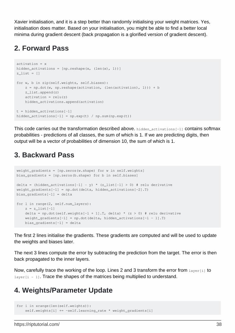
4. Weights/Parameter Update

for i in xrange(len(self.weights)): self.weights[i] += -self.learning_rate * weight_gradients[i]

https://riptutorial.com/ 38

self.biases[i] += -self.learning_rate * bias_gradients[i]

self.learning_rate specifies the rate at which the network learns. You don't want it to learn too fast, because it may not converge. A smooth descent is favoured for finding a good minima. Usually, rates between 0.01 and 0.1 are considered good.

Activation Functions

Activation functions also known as transfer function is used to map input nodes to output nodes in certain fashion.

They are used to impart non linearity to the output of a neural network layer.

Some commonly used functions and their curves are given below:

https://riptutorial.com/ 39

Sigmoid Function

The sigmoid is a squashing function whose output is in the range [0, 1].

The code for implementing sigmoid along with its derivative with numpy is shown below:

def sigmoid(z):

Hyperbolic Tangent Function (tanh)

The basic difference between the tanh and sigmoid functions is that tanh is 0 centred, squashing

You can easily use the np.tanh or math.tanh functions to compute the activation of a hidden layer.

ReLU Function

A rectified linear unit does simply max(0,x)

https://riptutorial.com/ 40

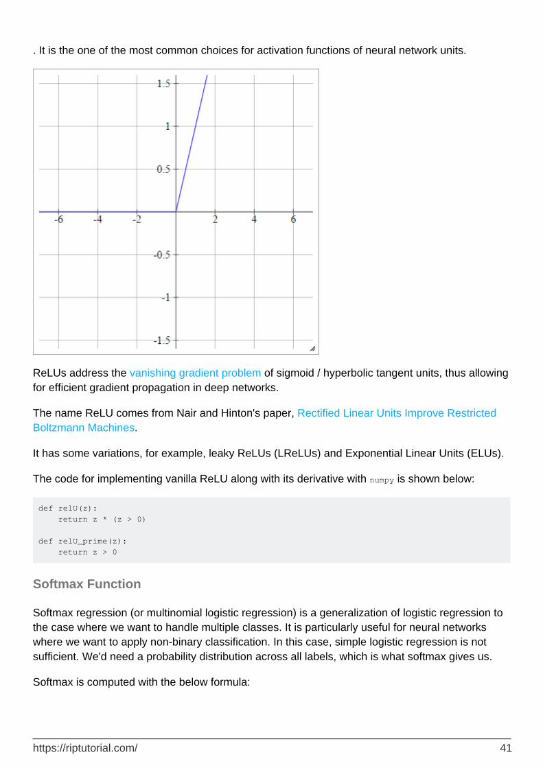
. It is the one of the most common choices for activation functions of neural network units.

ReLUs address the vanishing gradient problem of sigmoid / hyperbolic tangent units, thus allowing for efficient gradient propagation in deep networks.

The name ReLU comes from Nair and Hinton's paper, Rectified Linear Units Improve Restricted Boltzmann Machines.

It has some variations, for example, leaky ReLUs (LReLUs) and Exponential Linear Units (ELUs).

The code for implementing vanilla ReLU along with its derivative with numpy is shown below:

def relU(z): return z * (z > 0) def relU_prime(z): return z > 0

Softmax Function

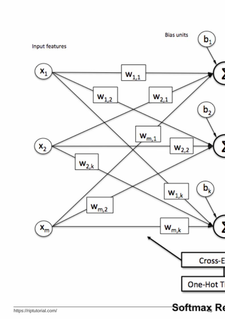
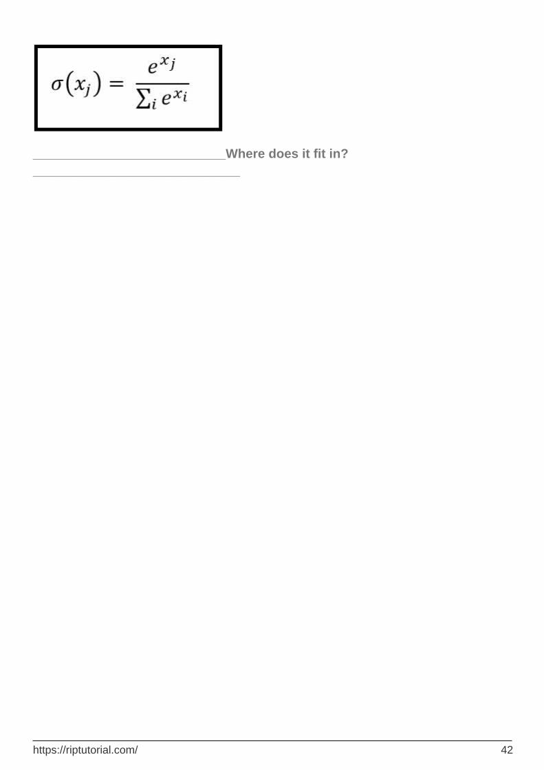
Softmax regression (or multinomial logistic regression) is a generalization of logistic regression to the case where we want to handle multiple classes. It is particularly useful for neural networks where we want to apply non-binary classification. In this case, simple logistic regression is not sufficient. We'd need a probability distribution across all labels, which is what softmax gives us.

Softmax is computed with the below formula:

https://riptutorial.com/ 41

___________________________Where does it fit in? _____________________________

https://riptutorial.com/ 42

https://riptutorial.com/ 43

To normalise a vector by applying the softmax function to it with numpy, use:

np.exp(x) / np.sum(np.exp(x))

Where x is the activation from the final layer of the ANN.

Read Neural Networks online: https://riptutorial.com/machine-learning/topic/2709/neural-networks

https://riptutorial.com/ 44

Chapter 10: Perceptron

Examples

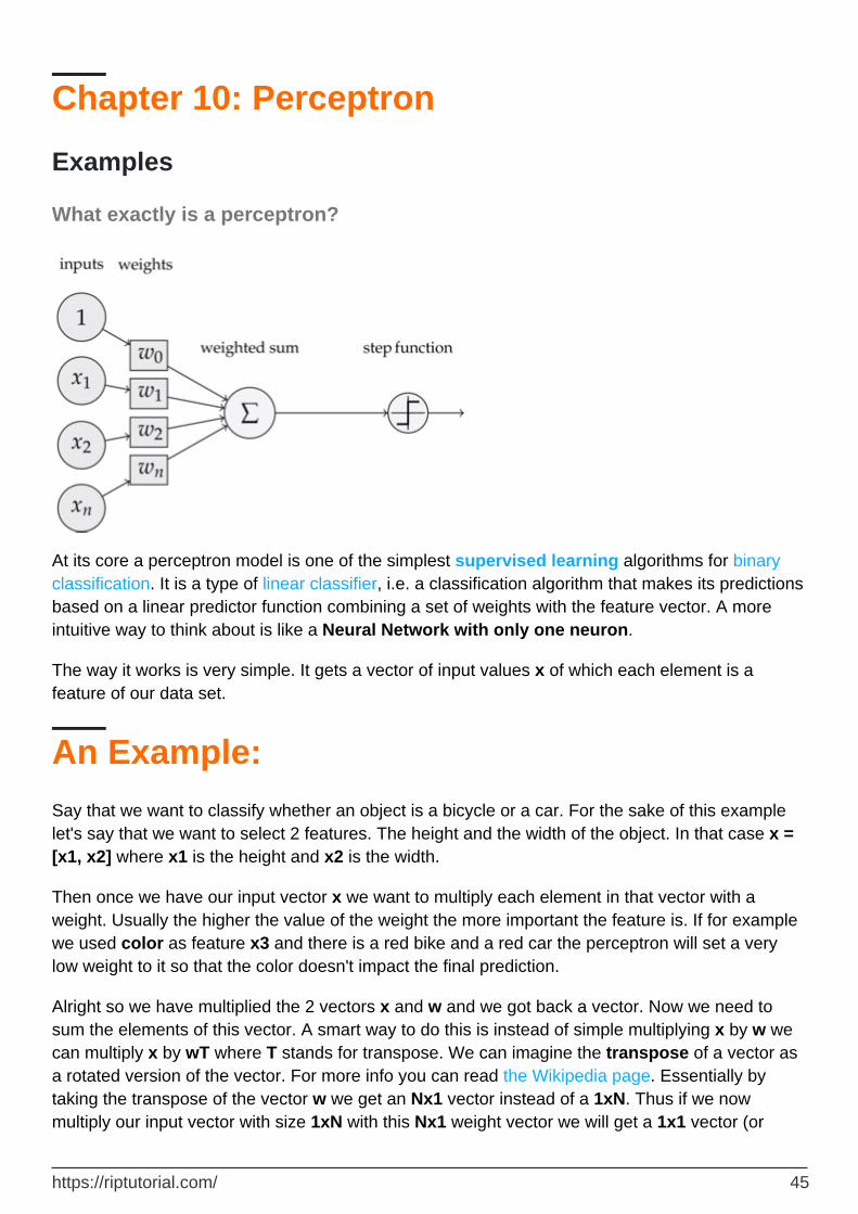
What exactly is a perceptron?

At its core a perceptron model is one of the simplest supervised learning algorithms for binary classification. It is a type of linear classifier, i.e. a classification algorithm that makes its predictions based on a linear predictor function combining a set of weights with the feature vector. A more intuitive way to think about is like a Neural Network with only one neuron.

The way it works is very simple. It gets a vector of input values x of which each element is a feature of our data set.

An Example:

Say that we want to classify whether an object is a bicycle or a car. For the sake of this example let's say that we want to select 2 features. The height and the width of the object. In that case x = [x1, x2] where x1 is the height and x2 is the width.

Then once we have our input vector x we want to multiply each element in that vector with a weight. Usually the higher the value of the weight the more important the feature is. If for example we used color as feature x3 and there is a red bike and a red car the perceptron will set a very low weight to it so that the color doesn't impact the final prediction.

Alright so we have multiplied the 2 vectors x and w and we got back a vector. Now we need to sum the elements of this vector. A smart way to do this is instead of simple multiplying x by w we can multiply x by wT where T stands for transpose. We can imagine the transpose of a vector as a rotated version of the vector. For more info you can read the Wikipedia page. Essentially by taking the transpose of the vector w we get an Nx1 vector instead of a 1xN. Thus if we now multiply our input vector with size 1xN with this Nx1 weight vector we will get a 1x1 vector (or

https://riptutorial.com/ 45

simply a single value) which will be equal to x1 * w1 + x2 * w2 + ... + xn * wn. Having done that, we now have our prediction. But there is one last thing. This prediction will probably not be a simple 1 or -1 to be able to classify a new sample. So what we can do is to simply say the following: If our prediction is bigger than 0 then we say that the sample belongs to class 1, otherwise if the prediction is smaller than zero we say that the sample belongs to the class -1. This is called a step function.

But how do we get the right weights so that we do correct predictions? In other words, how do we train our perceptron model?

Well in the case of the perceptron we do not need fancy math equations to train our model. Our weights can be adjusted by the following equation:

Δw = eta * (y - prediction) * x(i)

where x(i) is our feature (x1 for example for weight 1, x2 for w2 and so on...).

Also noticed that there is a variable called eta that is the learning rate. You can imagine the learning rate as how big we want the change of the weights to be. A good learning rate results in a fast learning algorithm. A too high value of eta can result in an increasing amount of errors at each epoch and results in the model doing really bad predictions and never converging. Too low of a learning rate can have as a result the model to take too much time to converge. (Usually a good value to set eta to for the perceptron model is 0.1 but it can differ from case to case).

Finally some of you might have noticed that the first input is a constant ( 1 ) and is multiplied by w0. So what exactly is that? In order to get a good prediction we need to add a bias. And that's exactly what that constant is.

To modify the weight of the bias term we use the same equation as we did for the other weights but in this case we do not multiply it by the input (because the input is a constant 1 and so we don't have to):

Δw = eta * (y - prediction)

So that is basically how a simple perceptron model works! Once we train our weights we can give it new data and have our predictions.

NOTE:

The Perceptron model has an important disadvantage! It will never converge (e.i find the perfect weights) if the data isn't linearly separable, which means being able to separate the 2 classes in a feature space by a straight line. So in order to avoid that it is a good practice to add a fixed number of iterations so that the model isn't stuck at adjusting weights that will never be perfectly tuned.

Implementing a Perceptron model in C++

https://riptutorial.com/ 46

In this example I will go through the implementation of the perceptron model in C++ so that you can get a better idea of how it works.

First things first it is a good practice to write down a simple algorithm of what we want to do.

Algorithm:

Make a the vector for the weights and initialize it to 0 (Don't forget to add the bias term)1. Keep adjusting the weights until we get 0 errors or a low error count.2. Make predictions on unseen data.3.

Having written a super simple algorithm let's now write some of the functions that we will need.

We will need a function to calculate the net's input (e.i x * wT multiplying the inputs time the weights)

•

A step function so that we get a prediction of either 1 or -1•And a function that finds the ideal values for the weights.•

So without further ado let's get right into it.

Let's start simple by creating a perceptron class:

class perceptron { public: private: };

Now let's add the functions that we will need.

class perceptron { public: perceptron(float eta,int epochs); float netInput(vector<float> X); int predict(vector<float> X); void fit(vector< vector<float> > X, vector<float> y); private: };

Notice how the function fit takes as an argument a vector of vector< float >. That is because our training dataset is a matrix of inputs. Essentially we can imagine that matrix as a couple of vectors x stacked the one on top of another and each column of that Matrix being a feature.

Finally let's add the values that our class needs to have. Such as the vector w to hold the weights, the number of epochs which indicates the number of passes that we will do over the training dataset. And the constant eta which is the learning rate of which we will multiply each weight update in order to make the training procedure faster by dialing this value up or if eta is too high we can dial it down to get the ideal result( for most applications of the perceptron I would suggest

https://riptutorial.com/ 47

an eta value of 0.1 ).

class perceptron { public: perceptron(float eta,int epochs); float netInput(vector<float> X); int predict(vector<float> X); void fit(vector< vector<float> > X, vector<float> y); private: float m_eta; int m_epochs; vector < float > m_w; };

Now with our class set. It's time to write each one of the functions.

We will start from the constructor ( perceptron(float eta,int epochs); )

perceptron::perceptron(float eta, int epochs) { m_epochs = epochs; // We set the private variable m_epochs to the user selected value m_eta = eta; // We do the same thing for eta }

As you can see what we will be doing is very simple stuff. So let's move on to another simple function. The predict function( int predict(vector X); ). Remember that what the all predict function does is taking the net input and returning a value of 1 if the netInput is bigger than 0 and -1 otherwhise.

int perceptron::predict(vector<float> X) { return netInput(X) > 0 ? 1 : -1; //Step Function }

Notice that we used an inline if statement to make our lives easier. Here's how the inline if statement works:

condition ? if_true : else

So far so good. Let's move on to implementing the netInput function( float netInput(vector X); )

The netInput does the following; multiplies the input vector by the transpose of the weights vector

x * wT

In other words, it multiplies each element of the input vector x by the corresponding element of the vector of weights w and then takes their sum and adds the bias.

(x1 * w1 + x2 * w2 + ... + xn * wn) + bias

bias = 1 * w0

https://riptutorial.com/ 48

float perceptron::netInput(vector<float> X) { // Sum(Vector of weights * Input vector) + bias float probabilities = m_w[0]; // In this example I am adding the perceptron first for (int i = 0; i < X.size(); i++) { probabilities += X[i] * m_w[i + 1]; // Notice that for the weights I am counting // from the 2nd element since w0 is the bias and I already added it first. } return probabilities; }

Alright so we are now pretty much done last thing we need to do is to write the fit function which modifies the weights.

void perceptron::fit(vector< vector<float> > X, vector<float> y) { for (int i = 0; i < X[0].size() + 1; i++) // X[0].size() + 1 -> I am using +1 to add the bias term { m_w.push_back(0); // Setting each weight to 0 and making the size of the vector // The same as the number of features (X[0].size()) + 1 for the bias term } for (int i = 0; i < m_epochs; i++) // Iterating through each epoch { for (int j = 0; j < X.size(); j++) // Iterating though each vector in our training Matrix { float update = m_eta * (y[j] - predict(X[j])); //we calculate the change for the weights for (int w = 1; w < m_w.size(); w++){ m_w[w] += update * X[j][w - 1]; } // we update each weight by the update * the training sample m_w[0] = update; // We update the Bias term and setting it equal to the update } } }

So that was essentially it. With only 3 functions we now have a working perceptron class that we can use to make predictions!

In case you want to copy-paste the code and try it out. Here is the entire class (I added some extra functionality such as printing the weights vector and the errors in each epoch as well as added the option to import/export weights.)

Here is the code:

The class header:

class perceptron { public: perceptron(float eta,int epochs); float netInput(vector<float> X); int predict(vector<float> X); void fit(vector< vector<float> > X, vector<float> y); void printErrors();

https://riptutorial.com/ 49

void exportWeights(string filename); void importWeights(string filename); void printWeights(); private: float m_eta; int m_epochs; vector < float > m_w; vector < float > m_errors; };

The class .cpp file with the functions:

perceptron::perceptron(float eta, int epochs) { m_epochs = epochs; m_eta = eta; } void perceptron::fit(vector< vector<float> > X, vector<float> y) { for (int i = 0; i < X[0].size() + 1; i++) // X[0].size() + 1 -> I am using +1 to add the bias term { m_w.push_back(0); } for (int i = 0; i < m_epochs; i++) { int errors = 0; for (int j = 0; j < X.size(); j++) { float update = m_eta * (y[j] - predict(X[j])); for (int w = 1; w < m_w.size(); w++){ m_w[w] += update * X[j][w - 1]; } m_w[0] = update; errors += update != 0 ? 1 : 0; } m_errors.push_back(errors); } } float perceptron::netInput(vector<float> X) { // Sum(Vector of weights * Input vector) + bias float probabilities = m_w[0]; for (int i = 0; i < X.size(); i++) { probabilities += X[i] * m_w[i + 1]; } return probabilities; } int perceptron::predict(vector<float> X) { return netInput(X) > 0 ? 1 : -1; //Step Function } void perceptron::printErrors() { printVector(m_errors); }

https://riptutorial.com/ 50

void perceptron::exportWeights(string filename) { ofstream outFile; outFile.open(filename); for (int i = 0; i < m_w.size(); i++) { outFile << m_w[i] << endl; } outFile.close(); } void perceptron::importWeights(string filename) { ifstream inFile; inFile.open(filename); for (int i = 0; i < m_w.size(); i++) { inFile >> m_w[i]; } } void perceptron::printWeights() { cout << "weights: "; for (int i = 0; i < m_w.size(); i++) { cout << m_w[i] << " "; } cout << endl; }

Also if you want to try out an example here is an example I made:

main.cpp:

#include <iostream> #include <vector> #include <algorithm> #include <fstream> #include <string> #include <math.h> #include "MachineLearning.h" using namespace std; using namespace MachineLearning; vector< vector<float> > getIrisX(); vector<float> getIrisy(); int main() { vector< vector<float> > X = getIrisX(); vector<float> y = getIrisy(); vector<float> test1; test1.push_back(5.0); test1.push_back(3.3);

https://riptutorial.com/ 51

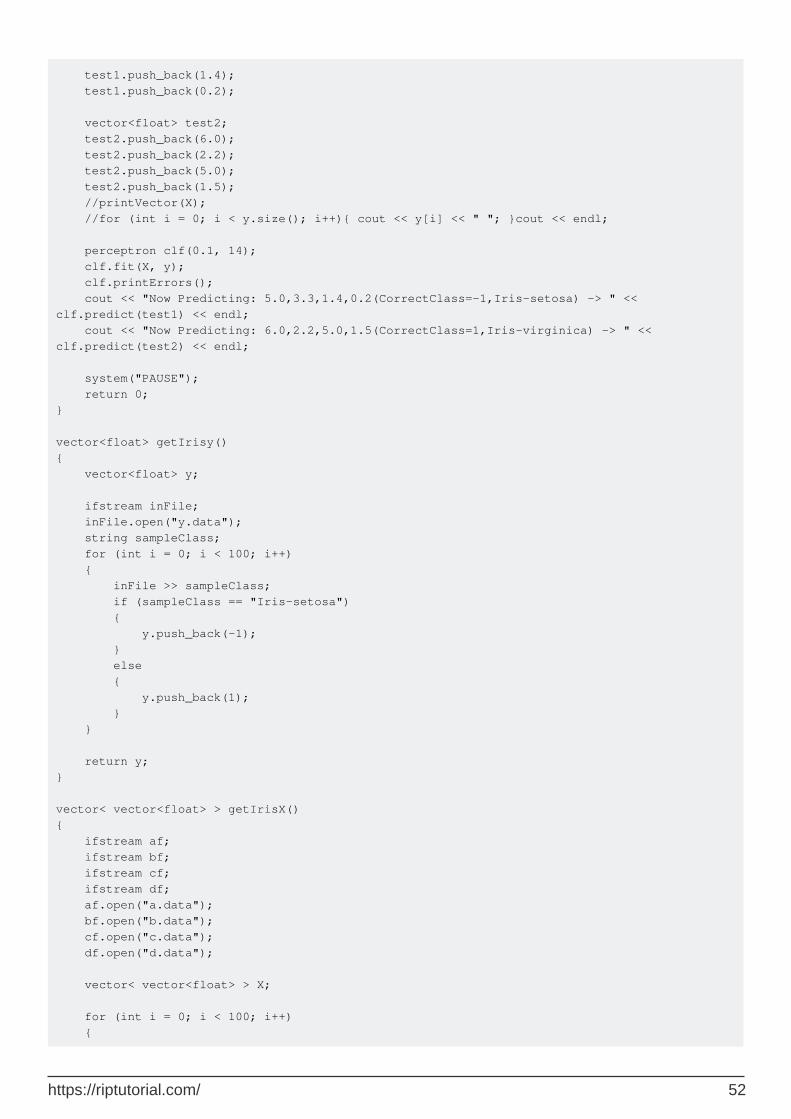
test1.push_back(1.4); test1.push_back(0.2); vector<float> test2; test2.push_back(6.0); test2.push_back(2.2); test2.push_back(5.0); test2.push_back(1.5); //printVector(X); //for (int i = 0; i < y.size(); i++){ cout << y[i] << " "; }cout << endl; perceptron clf(0.1, 14); clf.fit(X, y); clf.printErrors(); cout << "Now Predicting: 5.0,3.3,1.4,0.2(CorrectClass=-1,Iris-setosa) -> " << clf.predict(test1) << endl; cout << "Now Predicting: 6.0,2.2,5.0,1.5(CorrectClass=1,Iris-virginica) -> " << clf.predict(test2) << endl; system("PAUSE"); return 0; } vector<float> getIrisy() { vector<float> y; ifstream inFile; inFile.open("y.data"); string sampleClass; for (int i = 0; i < 100; i++) { inFile >> sampleClass; if (sampleClass == "Iris-setosa") { y.push_back(-1); } else { y.push_back(1); } } return y; } vector< vector<float> > getIrisX() { ifstream af; ifstream bf; ifstream cf; ifstream df; af.open("a.data"); bf.open("b.data"); cf.open("c.data"); df.open("d.data"); vector< vector<float> > X; for (int i = 0; i < 100; i++) {

https://riptutorial.com/ 52

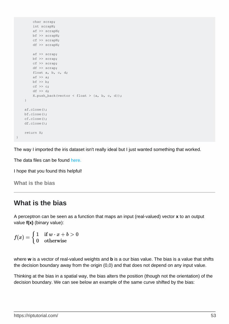
char scrap; int scrapN; af >> scrapN; bf >> scrapN; cf >> scrapN; df >> scrapN; af >> scrap; bf >> scrap; cf >> scrap; df >> scrap; float a, b, c, d; af >> a; bf >> b; cf >> c; df >> d; X.push_back(vector < float > {a, b, c, d}); } af.close(); bf.close(); cf.close(); df.close(); return X; }

The way I imported the iris dataset isn't really ideal but I just wanted something that worked.

The data files can be found here.

I hope that you found this helpful!

What is the bias

What is the bias

A perceptron can be seen as a function that maps an input (real-valued) vector x to an output value f(x) (binary value):

where w is a vector of real-valued weights and b is a our bias value. The bias is a value that shifts the decision boundary away from the origin (0,0) and that does not depend on any input value.

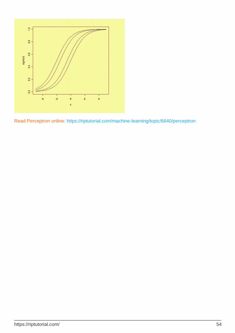
Thinking at the bias in a spatial way, the bias alters the position (though not the orientation) of the decision boundary. We can see below an example of the same curve shifted by the bias:

https://riptutorial.com/ 53

Read Perceptron online: https://riptutorial.com/machine-learning/topic/6640/perceptron

https://riptutorial.com/ 54

Chapter 11: Scikit Learn

Examples

A Basic Simple Classification Problem(XOR) using k nearest neighbor algorithm

Consider you want to predict the correct answer for XOR popular problem. You Knew what is XOR(e.g [x0 x1] => y). for example [0 0] => 0, [0 1] => [1] and...

#Load Sickit learn data from sklearn.neighbors import KNeighborsClassifier #X is feature vectors, and y is correct label(To train model) X = [[0, 0],[0 ,1],[1, 0],[1, 1]] y = [0,1,1,0] #Initialize a Kneighbors Classifier with K parameter set to 2 KNC = KNeighborsClassifier(n_neighbors= 2) #Fit the model(the KNC learn y Given X) KNC.fit(X, y) #print the predicted result for [1 1] print(KNC.predict([[1 1]]))

Classification in scikit-learn

1. Bagged Decision Trees

Bagging performs best with algorithms that have high variance. A popular example are decision trees, often constructed without pruning.

In the example below see an example of using the BaggingClassifier with the Classification and Regression Trees algorithm (DecisionTreeClassifier). A total of 100 trees are created.

Dataset Used: Pima Indians Diabetes Data Set

# Bagged Decision Trees for Classification import pandas from sklearn import cross_validation from sklearn.ensemble import BaggingClassifier from sklearn.tree import DecisionTreeClassifier url = "https://archive.ics.uci.edu/ml/machine-learning-databases/pima-indians-diabetes/pima-indians-diabetes.data" names = ['preg', 'plas', 'pres', 'skin', 'test', 'mass', 'pedi', 'age', 'class'] dataframe = pandas.read_csv(url, names=names) array = dataframe.values X = array[:,0:8] Y = array[:,8] num_folds = 10 num_instances = len(X)

https://riptutorial.com/ 55

seed = 7 kfold = cross_validation.KFold(n=num_instances, n_folds=num_folds, random_state=seed) cart = DecisionTreeClassifier() num_trees = 100 model = BaggingClassifier(base_estimator=cart, n_estimators=num_trees, random_state=seed) results = cross_validation.cross_val_score(model, X, Y, cv=kfold) print(results.mean())

Running the example, we get a robust estimate of model accuracy.

0.770745044429

2. Random Forest

Random forest is an extension of bagged decision trees.

Samples of the training dataset are taken with replacement, but the trees are constructed in a way that reduces the correlation between individual classifiers. Specifically, rather than greedily choosing the best split point in the construction of the tree, only a random subset of features are considered for each split.

You can construct a Random Forest model for classification using the RandomForestClassifier class.

The example below provides an example of Random Forest for classification with 100 trees and split points chosen from a random selection of 3 features.

# Random Forest Classification import pandas from sklearn import cross_validation from sklearn.ensemble import RandomForestClassifier url = "https://archive.ics.uci.edu/ml/machine-learning-databases/pima-indians-diabetes/pima-indians-diabetes.data" names = ['preg', 'plas', 'pres', 'skin', 'test', 'mass', 'pedi', 'age', 'class'] dataframe = pandas.read_csv(url, names=names) array = dataframe.values X = array[:,0:8] Y = array[:,8] num_folds = 10 num_instances = len(X) seed = 7 num_trees = 100 max_features = 3 kfold = cross_validation.KFold(n=num_instances, n_folds=num_folds, random_state=seed) model = RandomForestClassifier(n_estimators=num_trees, max_features=max_features) results = cross_validation.cross_val_score(model, X, Y, cv=kfold) print(results.mean())

Running the example provides a mean estimate of classification accuracy.

0.770727956254

3. AdaBoost

https://riptutorial.com/ 56

AdaBoost was perhaps the first successful boosting ensemble algorithm. It generally works by weighting instances in the dataset by how easy or difficult they are to classify, allowing the algorithm to pay or or less attention to them in the construction of subsequent models.

You can construct an AdaBoost model for classification using the AdaBoostClassifier class.

The example below demonstrates the construction of 30 decision trees in sequence using the AdaBoost algorithm.

# AdaBoost Classification import pandas from sklearn import cross_validation from sklearn.ensemble import AdaBoostClassifier url = "https://archive.ics.uci.edu/ml/machine-learning-databases/pima-indians-diabetes/pima-indians-diabetes.data" names = ['preg', 'plas', 'pres', 'skin', 'test', 'mass', 'pedi', 'age', 'class'] dataframe = pandas.read_csv(url, names=names) array = dataframe.values X = array[:,0:8] Y = array[:,8] num_folds = 10 num_instances = len(X) seed = 7 num_trees = 30 kfold = cross_validation.KFold(n=num_instances, n_folds=num_folds, random_state=seed) model = AdaBoostClassifier(n_estimators=num_trees, random_state=seed) results = cross_validation.cross_val_score(model, X, Y, cv=kfold) print(results.mean())

Running the example provides a mean estimate of classification accuracy.

0.76045796309

4. Stochastic Gradient Boosting

Stochastic Gradient Boosting (also called Gradient Boosting Machines) are one of the most sophisticated ensemble techniques. It is also a technique that is proving to be perhaps of the best techniques available for improving performance via ensembles.

You can construct a Gradient Boosting model for classification using the GradientBoostingClassifier class.

The example below demonstrates Stochastic Gradient Boosting for classification with 100 trees.

# Stochastic Gradient Boosting Classification import pandas from sklearn import cross_validation from sklearn.ensemble import GradientBoostingClassifier url = "https://archive.ics.uci.edu/ml/machine-learning-databases/pima-indians-diabetes/pima-indians-diabetes.data" names = ['preg', 'plas', 'pres', 'skin', 'test', 'mass', 'pedi', 'age', 'class'] dataframe = pandas.read_csv(url, names=names) array = dataframe.values X = array[:,0:8]

https://riptutorial.com/ 57

Y = array[:,8] num_folds = 10 num_instances = len(X) seed = 7 num_trees = 100 kfold = cross_validation.KFold(n=num_instances, n_folds=num_folds, random_state=seed) model = GradientBoostingClassifier(n_estimators=num_trees, random_state=seed) results = cross_validation.cross_val_score(model, X, Y, cv=kfold) print(results.mean())

Running the example provides a mean estimate of classification accuracy.

0.764285714286

Source: http://machinelearningmastery.com/ensemble-machine-learning-algorithms-python-scikit-learn/

Read Scikit Learn online: https://riptutorial.com/machine-learning/topic/6156/scikit-learn

https://riptutorial.com/ 58

Chapter 12: Supervised Learning

Examples

Classification

Imagine that a system want to detect apples and oranges in a basket of fruits. System can pick a fruit, extract some property of it (e.g weight of that fruit).

Suppose System has a Teacher! that teaches the system which objects are apples and which are oranges. This is an example of a supervised classification problem. It is supervised because we have labeled examples. It is classification because the output is a prediction of which class our object belongs too.

In this example we consider 3 features (properties/explanatory variables):

is weight of the selected fruit greater that .5gram1. is size greater than 10cm2. is the color is red3.

(0 mean No, and 1 means Yes)

So to represent an apple/orange we have a series(called vector) of 3 properties(often called a feature vector)

(e.g [0,0,1] mean that this fruit weight is Not greater that .5gram, and it's size is Not greater than 10cm and the color of it is red)

So, We pick 10 fruit randomly and measure their properties. The teacher (human) then labels each fruit manually as apple => [1] or orange => [2].

eg) Teacher select a fruit that is apple. The representation of this apple for system could be something like this: [1, 1, 1] => [1], This means that, this fruit has 1.weight greater that .5gram, 2.size greater than 10cm and 3. the color of this fruit is red and finally it is an apple(=> [1])

So for all of 10 fruits, the teacher label each fruit as apple[=>1] or orange[=>2] and the system found their properties. as you guess we have a series of vector(that called it matrix) to represent whole 10 fruits.

Fruit Classification

In this example, a model will learn to classify fruits given certain features, using the Labels for training.

Weight Color Label

0.5 green apple

https://riptutorial.com/ 59

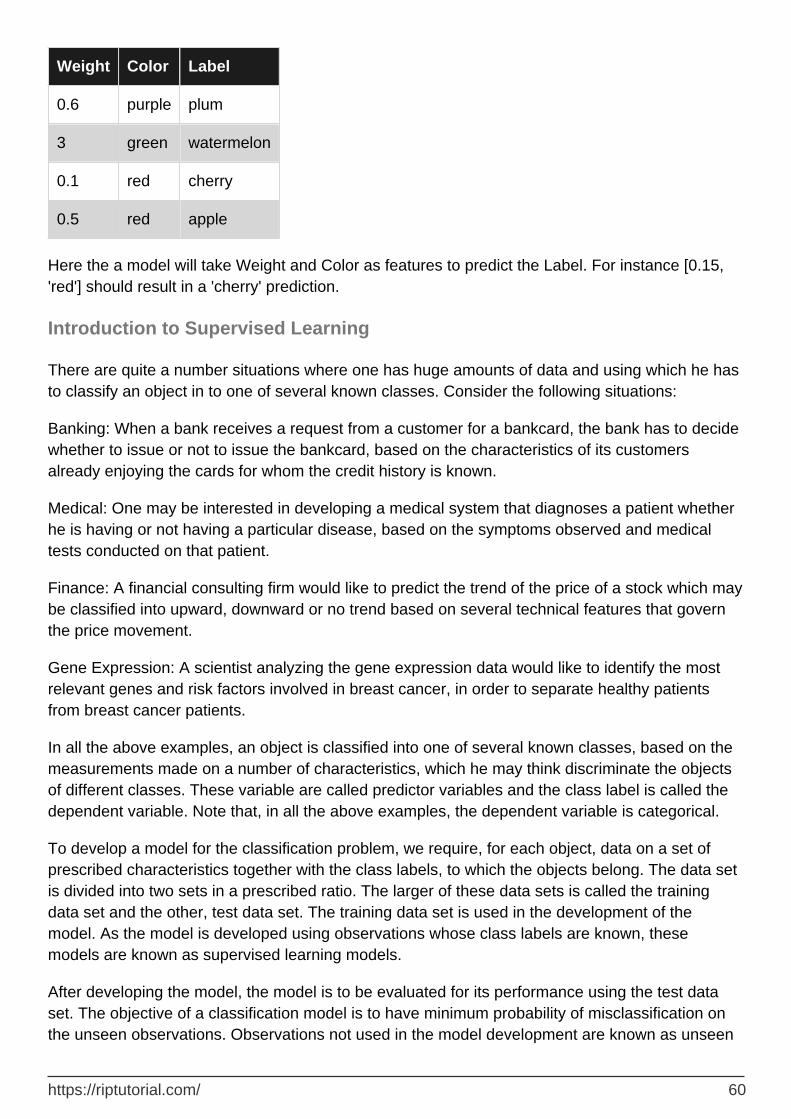
Weight Color Label

0.6 purple plum

3 green watermelon

0.1 red cherry

0.5 red apple

Here the a model will take Weight and Color as features to predict the Label. For instance [0.15, 'red'] should result in a 'cherry' prediction.

Introduction to Supervised Learning

There are quite a number situations where one has huge amounts of data and using which he has to classify an object in to one of several known classes. Consider the following situations:

Banking: When a bank receives a request from a customer for a bankcard, the bank has to decide whether to issue or not to issue the bankcard, based on the characteristics of its customers already enjoying the cards for whom the credit history is known.

Medical: One may be interested in developing a medical system that diagnoses a patient whether he is having or not having a particular disease, based on the symptoms observed and medical tests conducted on that patient.

Finance: A financial consulting firm would like to predict the trend of the price of a stock which may be classified into upward, downward or no trend based on several technical features that govern the price movement.

Gene Expression: A scientist analyzing the gene expression data would like to identify the most relevant genes and risk factors involved in breast cancer, in order to separate healthy patients from breast cancer patients.

In all the above examples, an object is classified into one of several known classes, based on the measurements made on a number of characteristics, which he may think discriminate the objects of different classes. These variable are called predictor variables and the class label is called the dependent variable. Note that, in all the above examples, the dependent variable is categorical.

To develop a model for the classification problem, we require, for each object, data on a set of prescribed characteristics together with the class labels, to which the objects belong. The data set is divided into two sets in a prescribed ratio. The larger of these data sets is called the training data set and the other, test data set. The training data set is used in the development of the model. As the model is developed using observations whose class labels are known, these models are known as supervised learning models.

After developing the model, the model is to be evaluated for its performance using the test data set. The objective of a classification model is to have minimum probability of misclassification on the unseen observations. Observations not used in the model development are known as unseen

https://riptutorial.com/ 60

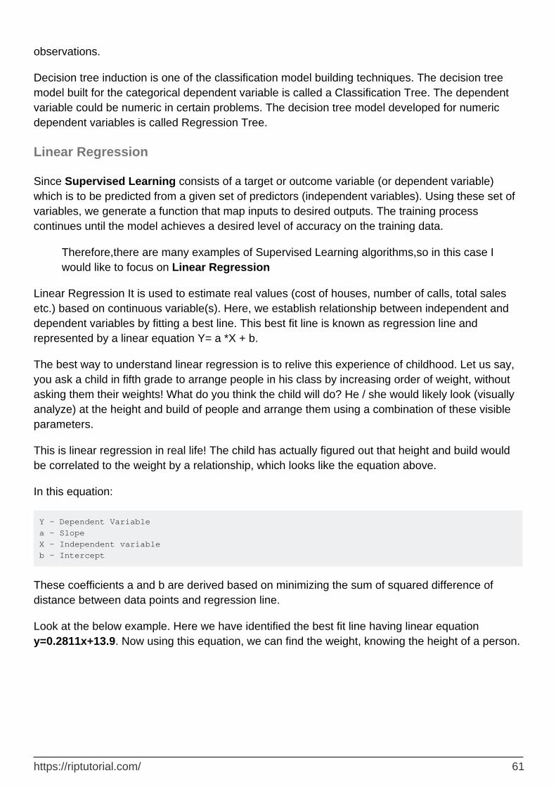
observations.

Decision tree induction is one of the classification model building techniques. The decision tree model built for the categorical dependent variable is called a Classification Tree. The dependent variable could be numeric in certain problems. The decision tree model developed for numeric dependent variables is called Regression Tree.

Linear Regression

Since Supervised Learning consists of a target or outcome variable (or dependent variable) which is to be predicted from a given set of predictors (independent variables). Using these set of variables, we generate a function that map inputs to desired outputs. The training process continues until the model achieves a desired level of accuracy on the training data.

Therefore,there are many examples of Supervised Learning algorithms,so in this case I would like to focus on Linear Regression

Linear Regression It is used to estimate real values (cost of houses, number of calls, total sales etc.) based on continuous variable(s). Here, we establish relationship between independent and dependent variables by fitting a best line. This best fit line is known as regression line and represented by a linear equation Y= a *X + b.

The best way to understand linear regression is to relive this experience of childhood. Let us say, you ask a child in fifth grade to arrange people in his class by increasing order of weight, without asking them their weights! What do you think the child will do? He / she would likely look (visually analyze) at the height and build of people and arrange them using a combination of these visible parameters.

This is linear regression in real life! The child has actually figured out that height and build would be correlated to the weight by a relationship, which looks like the equation above.

In this equation:

Y – Dependent Variable a – Slope X – Independent variable b – Intercept

These coefficients a and b are derived based on minimizing the sum of squared difference of distance between data points and regression line.

Look at the below example. Here we have identified the best fit line having linear equation y=0.2811x+13.9. Now using this equation, we can find the weight, knowing the height of a person.

https://riptutorial.com/ 61

Linear Regression is of mainly two types: Simple Linear Regression and Multiple Linear Regression. Simple Linear Regression is characterized by one independent variable. And, Multiple Linear Regression(as the name suggests) is characterized by multiple (more than 1) independent variables. While finding best fit line, you can fit a polynomial or curvilinear regression. And these are known as polynomial or curvilinear regression.

Just a hint on implementing linear regression in Python

#Import Library #Import other necessary libraries like pandas, numpy... from sklearn import linear_model #Load Train and Test datasets #Identify feature and response variable(s) and values must be numeric and numpy arrays x_train=input_variables_values_training_datasets y_train=target_variables_values_training_datasets x_test=input_variables_values_test_datasets # Create linear regression object linear = linear_model.LinearRegression() # Train the model using the training sets and check score linear.fit(x_train, y_train) linear.score(x_train, y_train) #Equation coefficient and Intercept print('Coefficient: \n', linear.coef_) print('Intercept: \n', linear.intercept_) #Predict Output predicted= linear.predict(x_test)

I have provided a glimpse on understanding Supervised Learning digging down to Linear Regression algorithm along with a snippet of Python code.

https://riptutorial.com/ 62

Read Supervised Learning online: https://riptutorial.com/machine-learning/topic/2673/supervised-learning

https://riptutorial.com/ 63

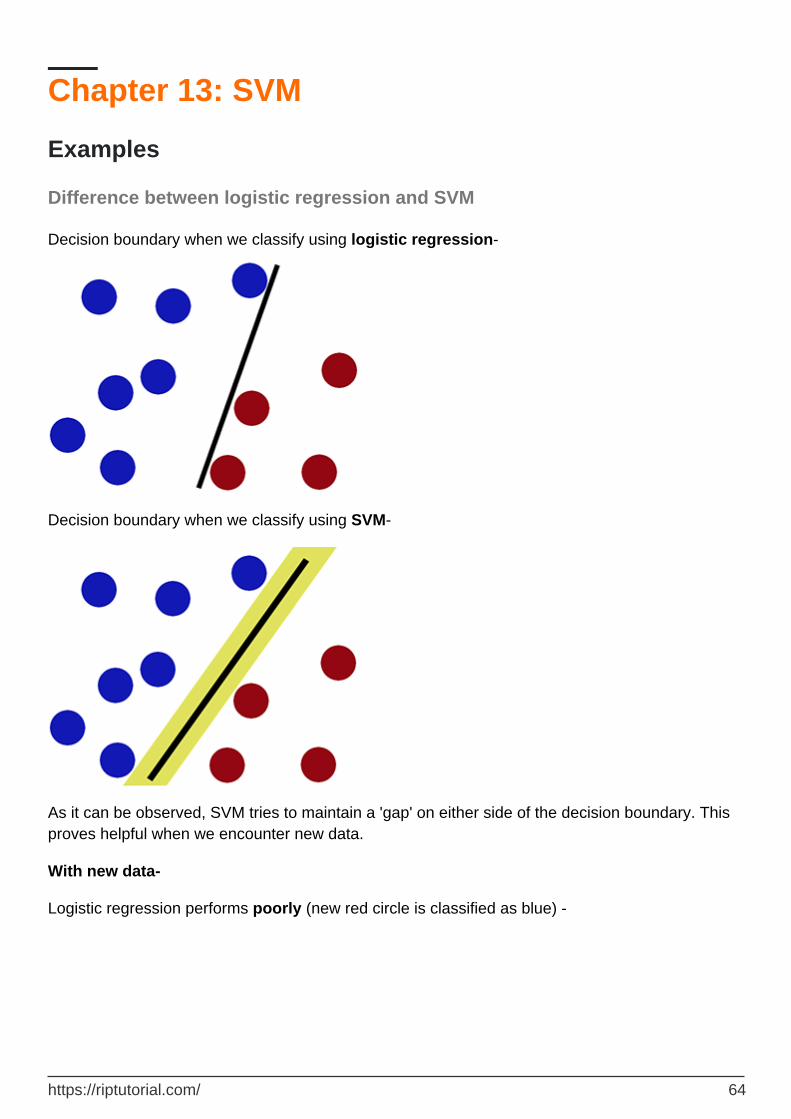
Chapter 13: SVM

Examples

Difference between logistic regression and SVM

Decision boundary when we classify using logistic regression-

Decision boundary when we classify using SVM-

As it can be observed, SVM tries to maintain a 'gap' on either side of the decision boundary. This proves helpful when we encounter new data.

With new data-

Logistic regression performs poorly (new red circle is classified as blue) -

https://riptutorial.com/ 64

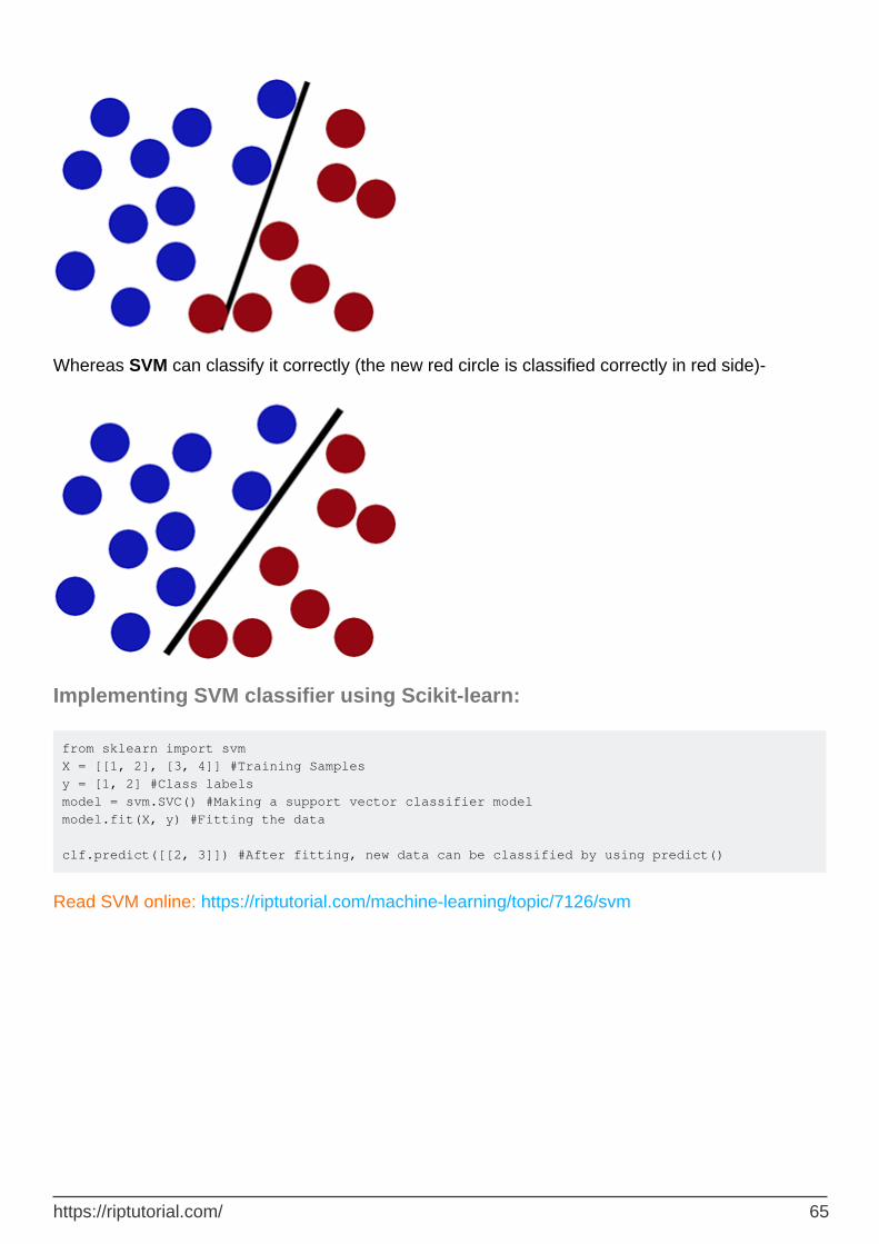
Whereas SVM can classify it correctly (the new red circle is classified correctly in red side)-

Implementing SVM classifier using Scikit-learn:

from sklearn import svm X = [[1, 2], [3, 4]] #Training Samples y = [1, 2] #Class labels model = svm.SVC() #Making a support vector classifier model model.fit(X, y) #Fitting the data clf.predict([[2, 3]]) #After fitting, new data can be classified by using predict()

Read SVM online: https://riptutorial.com/machine-learning/topic/7126/svm

https://riptutorial.com/ 65

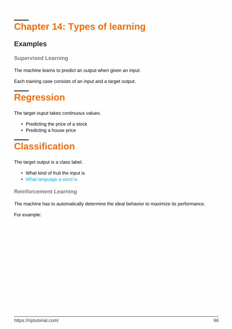
Chapter 14: Types of learning

Examples

Supervised Learning

The machine learns to predict an output when given an input.

Each training case consists of an input and a target output.

Regression

The target ouput takes continuous values.

Predicting the price of a stock•Predicting a house price•

Classification

The target output is a class label.

What kind of fruit the input is•What language a word is•

Reinforcement Learning

The machine has to automatically determine the ideal behavior to maximize its performance.

For example:

https://riptutorial.com/ 66

Using reinforcement learning you can also make a computer program that can complete a Mario level (MarI/O - Machine Learning for Video Games).

Unsupervised Learning

Unsupervised learning allows us to approach problems with little or no idea what our results should look like. We can derive structure from data where we don't necessarily know the effect of the variables.

The most common type of unsupervised learning is cluster analysis or clustering. It is the task of grouping a set of objects in such a way that object in the same group (cluster) are more similar to each other than to those in other groups.

There is also non-clustering unsupervised learning. An example thereof is identifying individual voices and music from a mesh of sounds. This is called the "Cocktail Party Algorithm".

Read Types of learning online: https://riptutorial.com/machine-learning/topic/10912/types-of-learning

https://riptutorial.com/ 67

Credits

S. No

Chapters Contributors

1Getting started with machine-learning

Aquib Javed Khan, Community, Dr. Cool, Drew, John Syrinek, Nikos Tavoularis, Piyush, Semih Korkmaz

2

An introduction to Classificiation: Generating several models using Weka

S van Balen

3 Deep Learning Martin W, Minhas Kamal, orbit, Thomas Pinetz

4 Evaluation MetricsDJanssens, Franck Dernoncourt, Sayali Sonawane, ScientiaEtVeritas

5

Getting started with Machine Learning using Apache spark MLib

Malav

6Machine learning and it's classification

Sirajus Salayhin

7Machine Learning Using Java

Arnab Biswas, Patel Sunil

8Natural Language Processing

quintumnia

9 Neural Networks cʟᴅsᴇᴇᴅ, dontloo, Dr. Cool, Franck Dernoncourt

10 Perceptron granmirupa, Martin W, Panos

11 Scikit Learn Masoud, RamenChef, Sayali Sonawane

12 Supervised Learningdraco_alpine, L.V.Rao, Martin W, Masoud, plumSemPy, quintumnia, shadowfox

13 SVM Alekh Karkada Ashok

14 Types of learning Martin W

https://riptutorial.com/ 68