MITSUBISHI ELECTRIC RESEARCH LABORATORIEShttps://www.merl.com

Machine Learning Methods for Predicting the FieldCompressive Strength of Concrete

DeRousseau, Mikaela A.; Laftchiev, Emil; Kasprzyk, Joseph R.; Balaji, Rajagopalan; Srubar III,Wil V.

TR2019-096 September 05, 2019

AbstractThis research analyzes the compressive strength behavior of field-placed concrete (hereintermed field concrete) as a function of mixture constituents. Compressive strength predictionof field concrete is inherently different and more challenging than that of laboratory concreteand merits its own analysis. In this work, we employ both field- and laboratory-obtained datato train and test machine learning models of increasing complexity for compressive strengthprediction. This training and testing scheme enables determination of the best-performingmodel specific to field concrete. In this work, the random forest machine learning modelfor predicting field compressive strength generated the best performance; the RMSE, MAE,and R2 values were 730 psi, 530 psi, and .51, respectively. The methodological reasons forvarying model performance are also examined. Finally, the ability of machine learning modelstrained on laboratory concrete data to predict the compressive strength of field concretemixtures is evaluated and compared to those models trained exclusively on field concretedata. The analysis shows that the hybridization of field and laboratory data for buildingpredictive models is a promising method for reducing common over-prediction issues causedby laboratory concrete models that are used in isolation

Construction and Building Materials

c© 2019 MERL. This work may not be copied or reproduced in whole or in part for any commercial purpose. Permissionto copy in whole or in part without payment of fee is granted for nonprofit educational and research purposes providedthat all such whole or partial copies include the following: a notice that such copying is by permission of MitsubishiElectric Research Laboratories, Inc.; an acknowledgment of the authors and individual contributions to the work; andall applicable portions of the copyright notice. Copying, reproduction, or republishing for any other purpose shallrequire a license with payment of fee to Mitsubishi Electric Research Laboratories, Inc. All rights reserved.

Mitsubishi Electric Research Laboratories, Inc.201 Broadway, Cambridge, Massachusetts 02139

Machine Learning Methods for Predicting the Field Compressive Strength of Concrete

M.A. DeRousseau 1, E. Laftchiev2, J.R. Kasprzyk 1, B. Rajagopalan1, W.V. Srubar III 1,†

1 Department of Civil, Environmental, and Architectural Engineering, University of Colorado Boulder,

ECOT 441 UCB 428, Boulder, Colorado 80309-0428 USA,

2Mitsubishi Electric Research Labs, 201 Broadway FL8, Cambridge, MA 02139

† Corresponding Author, T +1 303 492 2621, F +1 303 492 7317, E wsrubar@colorado.edu

Abstract

This research analyzes the compressive strength behavior of field-placed concrete (herein termed field

concrete) as a function of mixture constituents. Compressive strength prediction of field concrete is

inherently different and more challenging than that of laboratory concrete and merits its own analysis. In

this work, we employ both field- and laboratory-obtained data to train and test machine learning models

of increasing complexity for compressive strength prediction. This training and testing scheme enables

determination of the best-performing model specific to field concrete. In this work, the random forest

machine learning model for predicting field compressive strength generated the best performance; the

RMSE, MAE, and R2 values were 730 psi, 530 psi, and .51, respectively. The methodological reasons for

varying model performance are also examined. Finally, the ability of machine learning models trained on

laboratory concrete data to predict the compressive strength of field concrete mixtures is evaluated and

compared to those models trained exclusively on field concrete data. The analysis shows that the

hybridization of field and laboratory data for building predictive models is a promising method for

reducing common over-prediction issues caused by laboratory concrete models that are used in isolation.

Keywords: concrete; compressive strength; machine learning; prediction; statistical modeling

1. Introduction

The 28-day compressive strength of concrete is a critical design parameter for reinforced concrete

structures [1]. Empirical prescriptive- and performance-based mixture design methodologies remain the

conventional means to obtain concrete mixture design proportions that meet minimum 28-day

compressive strength requirements. However, numerical approaches for predicting the 28-day

compressive strength of concrete are emerging in the literature. Accurate numerical estimation of the 28-

day compressive strength of concrete is desirable because more precise prediction (1) provides assurance

of concrete quality, (2) reduces the number of concrete batches that are needed to be tested to meet

strength targets, and (3) enables a reduction in factors of safety. Recent computational studies have

demonstrated the ability of advanced statistical modeling techniques to numerically predict concrete

compressive strength for laboratory-mixed concrete, termed laboratory concrete herein [2]–[13].

However, prediction of the 28-day compressive strength of concrete placed in the field on an actual

construction site, termed field concrete herein, remains a challenge for the concrete industry due to

variable environmental conditions and other uncertainties

1.1 Prediction challenges for field concrete mixtures

Estimating the 28-day compressive strength of concrete is a multifaceted problem. Complex physical and

chemical interactions occur between concrete constituents, which, in turn, affect compressive strength.

Therefore, nonlinear mathematical models are advantageous for accurately capturing all phenomena. As

an example, consider the following physically intuitive correlations: compressive strength decreases

(nonlinearly) as the water-to-cement ratio (w/c) increases [14], [15], while increasing air content for

improved workability and freeze-thaw resistance reduces compressive strength [16]. Other correlations

have not been as intuitively deduced to-date. For example, it is well known that the proportion of coarse-

to-fine aggregate affects compressive strength, but the relationship has not been precisely determined due

to confounding factors, such as particle size distribution, aggregate angularity, and water demand. Coarse

aggregate, for example, may vary in nominal size, grading, chemical composition, shape, surface texture,

and absorptivity [17]; these properties can impact the strength of the interfacial bonds between the

aggregate and mortar, which, in turn, affect the compressive strength of concrete. Furthermore, the

addition of supplementary cementitious materials (SCMs), like fly ash, slag, and silica fume, also

introduce new, complex, and nonlinear relationships to compressive strength because of complex factors,

such as fineness, chemical variability, and pozzolanic reactivity [18], [19]. Additionally, the fineness and

mineral composition of fly ash and slag can be highly variable, depending on the original industrial

source and additional processing steps [20].

The conditions of the job site at which field concrete is mixed and placed are also highly variable and

lead to high variability in field compressive strength compared to laboratory concrete. For instance, it is

commonplace for the environmental conditions at construction sites to be loosely controlled. Here,

temperature, humidity, and inclement weather can all affect concrete curing and the final compressive

strength [21], [22]. Such variabilities do not exist in laboratory concrete mixing, which suggests that

accurate prediction of the compressive strength of field concrete is a more challenging problem compared

to compressive strength prediction of laboratory concrete.

1.2 Machine learning methods for compressive strength prediction Because of the physical limitations described above, there is growing interest in predicting concrete

compressive strength using machine learning (ML) models for both field and laboratory concrete

mixtures [23], [24]. ML models predict compressive strength (i.e., the target variable) from the types and

quantities of the mixture ingredients (i.e., the input variables). Using pairs of data of the form [input

variables, target variable], a model is trained from a collected dataset and learns the relationship between

the target and input variables without constraint on prior intuitive understanding. The vast majority of this

type of research has been performed on laboratory concrete, which, as discussed, suggests limitations on

the actual usefulness of these models for predicting the compressive strength of field concrete, given the

myriad of convoluting factors.

Prior research in ML methods for compressive strength prediction has been limited to testing ML

methods using laboratory data to determine best-possible prediction models for concrete compressive

strength. A particularly popular ML algorithm is artificial neural networks (ANNs). The first study of

ANNs by Yeh et al. [25] employed ANNs on a dataset of over 1000 laboratory concrete mixture designs.

Since then, other researchers have reported ANN studies with coefficients of determination (R2) of up to

0.999 [2]–[8], [10], [26]–[28]. However, a significant number of ANN studies employ less than 100

experimental data points, which may not sufficiently sample the predictor variable space. While ANNs

are a flexible and powerful ML method, it suffers from the need to train a large number of parameters.

For small datasets (as is common for field concrete), ANNs can quickly overfit the data, which leads to

strong training set performance but poor generalization performance on new datasets. Other ML methods

that appear in the literature include support vector machines (SVM) [25], [26] and decision tree-based

models [13], [29]. Studies that employ these methods are less common than ANN studies, due to the

historical alignment of compressive strength prediction and ML methods.

Some narrower-scope prediction studies that used ML have focused on modeling concrete mixtures

that contain particular mixture ingredients, such as fly ash [28], blast-furnace slag [30], recycled

aggregate [31], silica fume [32], and metakaolin [33]. This body of research generates models that are

useful for predicting compressive strength when specific constituents are included. However, this

approach narrowly tailors the model to the particular dataset and, thus, is less useful when either mixture

ingredients or external conditions (possibly unmeasured) may change.

A recent study by Young et al. considered field concrete data and compared the predictive

performance of four ML models for predicting both field and laboratory concrete [23]. This study found

that variance can be significantly better explained in the laboratory concrete dataset, which is compatible

with the idea that laboratory concrete has fewer uncontrolled variables. The study determined that the

four ML methods investigated exhibited equivalent predictive performance for field concrete – a

somewhat unintuitive result, given that the four methods employed do not share common assumptions

about the underlying data. In this study, it is also of note that the laboratory and field datasets contained

different mixture ingredients (i.e., input variables). For example, the laboratory concrete dataset included

blast-furnace slag, while the field concrete dataset does not, making an apples-to-apples comparison

difficult between models for both laboratory and field concrete.

1.3. Innovative contribution/knowledge gaps Despite a large body of research in this area of study, the challenge of training a ML model for accurate

prediction of concrete compressive strength remains relevant. More specifically, two significant gaps

exist in the literature. First, prior studies are not well-grounded in best-practice methods of the ML

community. The standard procedure in ML is to generate a pipeline of methods that increase in

complexity [34]. The reason for this is two-fold: (1) while powerful, ML methods often search a large

model space and may miss simple solutions recognized by the researcher and (2) the failure of simpler

models is typically caused by a failure in model assumptions that reveals previously hidden details about

the data interactions and non-linear behavior observed in the system. These failures can thus be used to

inform the appropriate choice of ML tools for further development. Second, consensus on the best model

architectures for predicting the compressive strength of field concrete has not yet been reached.

To this end, this study aims to address the aforementioned knowledge gaps and is particularly focused

on approaches for accurate prediction of the compressive strength of field concrete. First, we employ the

standard ML procedure of testing models of increasing complexity in order to determine the best-

performing model for field concrete. This procedure enables us build on past research by discussing why

certain ML methods are particularly well-suited for the concrete compressive strength prediction problem.

The field concrete dataset in this study contains 1681 concrete mixtures and was collected by the

Colorado Department of Transportation (CDOT). The laboratory concrete dataset in this study was

obtained from the University of California, Irvine Machine Learning Repository, which contains data for

more than 1000 mixtures [35].

Following the analysis of the field concrete dataset we evaluate the ability of ML models learned on

laboratory concrete data to predict the compressive strength of field concrete mixtures. For this analysis,

we perform the same ML procedure for the laboratory data and select the best-performing model. This

model is then used to predict the compressive strength of field concrete mixtures and the relative model

performance is analyzed. It is hypothesized that the laboratory ML model performance will be less-than

satisfactory for predicting field compressive strength. Consequently, this work includes an analysis of

laboratory models that are supplemented with varying percentages of field data in order to determine if

such hybridized datasets can improve performance of laboratory concrete models.

2. Machine Learning (ML) Methods

As discussed in the introduction, this paper builds a pipeline of ML methods with increasing complexity,

such that the underlying structure in the training data can be stepwise analyzed. First, in Section 2.1, we

describe the ML methods used in the pipeline. We introduce linear methods (i.e., linear regression,

polynomial regression), transformed linear methods (i.e., kernelized support vector regression, kernelized

Gaussian process regression), and non-linear methods (i.e., regression trees, boosted trees, random

forest). In general, simple models are introduced first, and subsequent models increase in complexity. The

simplest methods (e.g., linear regression) tend to require the most assumptions about the underlying data

structure, and the most complex methods (e.g., boosted trees) require few assumptions about the

underlying structure of the data. Second in Section 2.2, we analyze the utility of predictive models trained

on laboratory concrete data for predicting field concrete strength. Third, in Section 2.3, we introduce the

performance measures used to evaluate the effectiveness of each model: the coefficient of determination

(R2), root mean squared error (RMSE), and mean absolute error (MAE). Last, in Section 2.4, overfitting is

discussed, which occurs when a model not only captures the desired qualities in the data, but also begins

to exactly model the training data itself. An overfitted model is undesirable because it lowers the

predictive performance on “unseen” testing data. In other words, overfitted models do not generalize well

to real-world cases. In this analysis, we describe and utilize nested cross-validation as a means reduce

overfitting. Reserved testing data is used for final determination of the best-performing model.

2.1 ML Methods

All models were created in the R Project for Statistical Computing [36]; in addition, Table 1 lists the ML

methods employed in this study, as well as the specific package and function used for model training. For

each ML method, we discuss parameter tuning and the intuitive meaning of the parameters.

Table 1. ML models and corresponding R packages used in this study.

Model Type R Package R Function

Linear Methods

Linear regression stats lm

Polynomial regression stats lm

Transformed Linear Methods

Kernelized support vector

regression

kernlab ksvm

Kernelized Gaussian process kernlab gausspr

Non-Linear Methods

Regression trees rpart rpart

Random forest randomForest randomForest

Boosted trees gbm gbm

2.1.1 Linear Regression

The simplest model to apply and analyze is linear regression. In addition to providing useful

understanding of the data, linear regression also serves as a good baseline from which other techniques

can be evaluated. Linear regression is a model that describes the output (target) variable as a linear

combination of the predictor variables [37]. This linear combination is a hyperplane in N-dimensional

space, where N is the number of coefficients in the model. The model solution is the hyperplane that

minimizes the squared error between the observed output and the predicted output. Mathematically, the

solution is described as:

!" = #$%, Eq. 1

where x is the input vector, β is the N-dimensional vector of coefficients (parameters) for the linear

model, and !" is the predicted output variable from the model. The underlying assumption in linear

regression is that the relationship between the predictor variables and the output variable is linear.

Moreover, the model assumes that predictor variables are independent from one another, and the resulting

residuals, the difference between the predicted and observed output variables, are both homoscedastic

(i.e., have constant variance) and normally distributed. When these assumptions are violated, it indicates

that a linear model is not appropriate. When such violations occur, it is reasonable to use transformations

on the input data to try to reduce or eliminate the violation in assumptions. Failure of such methods to

improve the resulting model error and reduce violation of the assumptions means that the dataset requires

more complex non-linear models.

2.1.2 Multivariate Polynomial Regression

Multivariate polynomial regression (called polynomial regression in this study) uses nth degree

polynomials of the input variables to predict the output variable. Polynomial regression is a generalization

of Eq. 1; however, each x term may be: (1) an original predictor variable (e.g., &'), (2) a pure higher-order

term of one predictor variable (e.g., &'(), or (3) an interaction term between two or more predictor

variables (e.g., &'&)))

A generalized example of an expanded second-order polynomial solution with two predictor variables

(for simplicity) is described by:

!" = *+ , *'&' , *)&) , *''&') , *))&)) , *')&'&)- Eq. 2

The transformation of the predictor variables allows for modeling of higher-order relationships and

modeling interactions between the input variables; Eq. 2, for example, shows a parabolic relationship.

When the original predictor variables are transformed, they are called “features.” This term, also

commonly applied to all input variables of the models, denotes the fact that the inputs have been

transformed from their original space. In this analysis, polynomials up to third-order are employed, where

third order is chosen due to limits in computational power. Since polynomial regression is a form of linear

regression, the same assumptions are required—more specifically, independence of the input features,

homoscedasticity of the residuals, and normality of the residuals. Note, however, these assumptions apply

to the transformed features and not the original data space.

2.1.3 Kernalized Regression Methods

Kernalized regression methods utilize two mathematical concepts applied in tandem – a transformation of

the predictor variables and the pairing of the new predictors with a regression method. These pairings can

then be analyzed in order to determine which (if any) kernel and regression assumptions fit the data well.

Kernels are a set of transformations that can be used to map the original predictor variable space to a

high-dimensional feature space [34]. Here, this mapping is more complex than the polynomial mappings

in the previous section, and all mappings are the result of extensive previous research effort [38]. Each

kernel has its own set of tuning parameters that must be optimized. This paper compares four kernel

transformations, including: linear kernel, radial basis function (RBF) kernel, sigmoid kernel, and

polynomial kernels (up to order 4). The model order of the polynomial kernels is only limited by the

available computational power.

Kernel transformations have the form:

./#0 #12 = 34/#20 4/#526 Eq. 3

where k is the kernel function, x and x’ are N-dimensional input vectors (N is the number of predictor

variables), and 4 is a mapping from m dimensions to an m-dimensional space. Note that 34/#20 4/#526 denotes the inner product between the two mappings and can be thought of as a measure of similarity

between the two transformed vectors. The kernel tuning parameters are optimized in tandem with the

optimization of a regression model. This optimization is discussed below. Table 2 provides the kernel

transformation equations and kernel tuning parameters used in this study.

Table 2. Kernel Transformation equations and tuning parameters

Name Kernel Transformation Tuning Parameters

Linear ./#0 #12 = 3#0 #16 n/a

Radial Basis Function ./#0 #12 = exp-/789: 7#19)2 8

Polynomial ./#0 #12 = /83#0 #16 , ;2< 8, r, and d

The transformed variables (features) can be utilized with any regression method. The concept here is that

parameters for both the kernel transformations and the regression methods are tuned simultaneously such

that the cross-validated model error is minimized. When there are multiple tuning parameters, a grid

search technique is employed in order to find near-optimal parameter values. In this paper, two kernalized

regression methods are tested: support vector regression and Gaussian process regression.

Support vector regression (SVR) is a version of support vector machines (SVM) used for regression

purposes (rather than classification) [39]. The regression model generated by SVR depends on only a

subset of the dataset, and these data points are deemed support vectors. When an SVR model is trained,

support vectors are the points from the dataset that produce error values (>) larger than a prescribed

threshold value. SVR model training generates values for βm (the coefficients for the transformed support

vectors) and β0 (the intercept). This occurs via minimization of Eq. 4 using gradient descent:

min?@/*A0 *+2 = B C/!D 7 !"2 , E)

FDG' B*A) Eq. 4

Here, V(r) is the prescribed error measure, y is the observed target variable, and H is a regularization

parameter that serves as a degree of importance given to large error values. When H increases, large errors

are more greatly penalized in the model; this parameter can be tuned using cross-validation. In this study

the SVR is paired with the aforementioned kernel transformations in order to examine the utility of

transformations of the predictor variables.

The second regression method that is employed with the kernel-transformed data is Gaussian process

regression (GP). GP can be thought of as the Bayesian interpretation of linear regression. Rather than

assuming that the relationship between the predictor variables and the target variable has the prescribed

linear functional form (e.g. !" = #$%), GP simply assumes that the data can be represented as a sample

from a multivariate Gaussian distribution and that the mean of this distribution is zero. This approach is

“less parametric” in the sense that the model is more loosely defined. Using GP, the predictions of the

target variable are made using the conditional probability, I/!J|K2. In short: given the data, how likely is

a certain prediction for !J? Here, note the subtle difference between !" and !J. !" represents a predicted

target variable from a model, and !J represents a distribution of possible outputs from the model. In the

case of GP, !" is the expected value of !J,--L[!J] = L[!J|K]. Given the assumed Gaussian distribution, the matrix of all predictor variables in the dataset (M), the

output vector (y) and the new matrix of data inputs, the goal is to make a prediction on the new set of data

points (#J). The derived conditional distribution has the form,

!J|K-~-N/OJOP'K0 -OJJ 7OJOP'OJ$20 Eq. 5

where O, OJ, and OJJ are the covariance matrices resulting from ./#0 #52, ./#J0 #52, and ./#J0 #J52, respectively. The prediction, !", is the expected value of this distribution, which can be reduced to the

equation below.

!" = OJOP'K Eq. 6

Since GP employs only the assumption of a Gaussian distribution and the covariance matrices for model

formulation, no tuning parameters are necessary for this regression method beyond those required for the

choice of kernel. The performance of GP allows us to assess the veracity of the Gaussian distribution

assumption for the data under multiple different transformations of the predictor variables. If none of the

above regression methods can adequately model the output variable, models with no linearity assumptions

(e.g. regression trees, artificial neural networks) are reasonable model options consider.

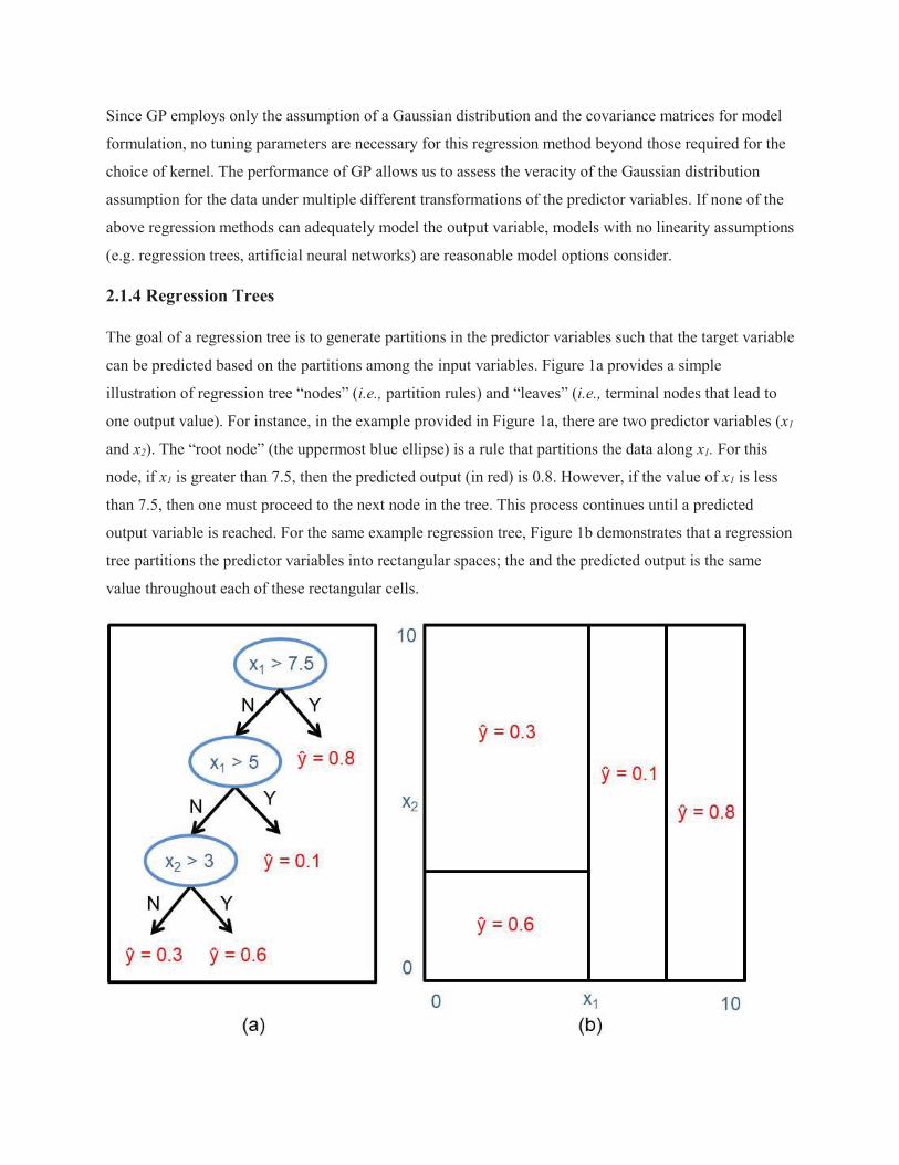
2.1.4 Regression Trees

The goal of a regression tree is to generate partitions in the predictor variables such that the target variable

can be predicted based on the partitions among the input variables. Figure 1a provides a simple

illustration of regression tree “nodes” (i.e., partition rules) and “leaves” (i.e., terminal nodes that lead to

one output value). For instance, in the example provided in Figure 1a, there are two predictor variables (x1

and x2). The “root node” (the uppermost blue ellipse) is a rule that partitions the data along x1. For this

node, if x1 is greater than 7.5, then the predicted output (in red) is 0.8. However, if the value of x1 is less

than 7.5, then one must proceed to the next node in the tree. This process continues until a predicted

output variable is reached. For the same example regression tree, Figure 1b demonstrates that a regression

tree partitions the predictor variables into rectangular spaces; the and the predicted output is the same

value throughout each of these rectangular cells.

Figure 1: (a) Diagram of an example regression tree model with two predictor variables, x1 and x2. (b)

This diagram shows the same decision tree using the two predictor variables as axes. It helps visualized

the rectangularity of the target variable predictions when simple regression trees are employed. Within

each rectangle the predicted target variable would be the same.

Training a regression tree is performed by selecting partitions in succession using a criterion of variance

reduction in the target variable [40]. Since each successive partition is always chosen such that the

variance of the target variable is reduced, regression trees are prone to overfitting the data. To prevent

overfitting, a variety of regularization techniques can be employed. This study minimizes the cost

complexity function, which places a penalty for each additional node that is selected for the model. As

shown below, the cost complexity function QR/S2 has two terms that influence its value:

QR/S2 = Q/S2 , T J U/S2, Eq. 7

Where Q/S2 is the training error, U/S2 is the number of leaves in the regression tree, and T is the

regularization parameter that is determined via cross-validation [41]. In Section 2.3 the cross-validation

procedure used in this study is thoroughly discussed.

Regression trees have the advantage that they do not assume linearity in the data, and, therefore, no

complex data transformations are needed. Overall, this approach is simpler than linear methods, but it

requires careful consideration so as not to overfit the data. Regression trees also implicitly select

variables, which means that a trained regression tree will show variables that have more importance for

predicting the target variable in earlier nodes in the tree. Lastly, regression trees are interpretable and can

provide some insight on the dataset being analyzed.

A disadvantage of simple regression trees is that they suffer from model instability; in other words, small

changes to the dataset might create a completely different set of partitions, and, consequently does not

lead to the best-performing model. For this reason, more complicated tree-based methods are often

considered that are more stable. Random forest and boosted trees are examples of more complex tree-

based methods that aim to reduce this instability and are discussed in the subsequent sections.

2.1.5 Random Forest

Random forest is a method that builds an ensemble of regression trees in order to reduce the instability of

individual trees. Random forest utilizes two strategies for improving the instability issue. First, it employs

the concept of “bootstrap aggregation” (sampling with replacement) in order to generate many similar

datasets that were sampled from the same original dataset. These datasets each lead to an individual tree

within the ensemble. Second, it incorporates randomness during tree-learning in order to reduce the

correlation between each tree within the ensemble. For instance, when generating new nodes (for

individual trees within the random forest), only a subset of the original predictor variables is selected as

the set of candidate variables on which to partition the data. The variable value that minimizes variance in

the output from these randomly selected predictors is the variable selected for that node. This process is

repeated for all nodes in a regression tree and then for all regression trees in the random forest. For a

random forest model, the tuning parameters are: the number of randomly selected predictors (k), the

number of individual trees that are trained (n), and the tree depth (d) [42].

The advantage of the random forest method is that it significantly reduces the instability of simple

regression trees. Furthermore, this method has been shown to minimize correlation between trees

compared to other tree-ensemble methods (e.g. “bagging trees” that use only bootstrap aggregation and

not random variable selection) [40]. One disadvantage of random forests is their reduction in

interpretability compared to simple regression trees; random forests cannot be easily visualized and

individual trees are often not good predictive models on their own. However, variable importance plots

can reveal the relative importance of predictor variables.

2.1.6 Boosted Trees

Like random forest, boosted trees are an ensemble method for dealing with the instability and poor

predictive performance of simple regression trees. Generally, the concept of “boosting” is an ensemble

strategy that can be used to improve weak learning algorithms (e.g. regression trees) [43], [44]. Boosting

can be applied to any weak learning algorithm but is commonly utilized for regression trees. The main

concept of boosting is to build a model using the weak learning algorithm. Then another model is learned

on the residuals from the first model. This step of model-building on the previous model’s residuals is

repeated for a set number of iterations. Therefore, a boosted tree is simply a model where the weak

learning algorithm used in each iteration is a regression tree.

Unlike random forest in which all trees are of the same importance, boosted trees are hierarchical,

meaning that each tree layer is constructed recursively. The tuning parameters for boosted trees are: the

number of trees, the interaction depth (maximum number of nodes per tree), the minimum number of

observations per node (a stopping criteria used to prevent trees that have only one observation at each

leaf), and the shrinkage rate (the rate at which the impact of each additional tree is reduced).

Boosted trees are similar to random forest in their advantages and disadvantages. Boosted trees tend to

have high predictive performance on highly nonlinear datasets and can be successful on problems where

there is unequal importance of predictor variables [34]. One disadvantage of boosted trees is that this

method has low interpretability; it is difficult to gain much intuition of the patterns that the model has

learned or to determine why a boosted tree model is successful (or not) at predicting the target variable.

This means that a strong ML pipeline must be used to train boosted trees to ensure that the approach has

not overfit the data.

2.2 Testing of Laboratory and Hybrid Models for Field Concrete Strength Prediction

2.2.1 Laboratory Models

As was discussed in the introduction, many studies in the literature have developed ML models for

predicting concrete compressive strength using laboratory concrete datasets. While these laboratory

models report high predictive performance [2], [4]–[8], [10], [26], [27], it has not yet been tested whether

they are useful for predicting the compressive strength of field concrete. A significant novelty of this

study is that laboratory models are tested to determine if they are, in fact, useful for predicting

compressive strength when presented with other datasets – namely, field concrete data.

One issue preventing the direct testing of laboratory ML models from the literature is the use of concrete

age as a predictor variable. In other studies, age is a convenient predictor variable because it can explain a

high percentage of variance in compressive strength data. In other words, removing age as a predictor and

using only the final compressive strength as the output causes the compressive strength problem to be

significantly more difficult (i.e., model performance measures tend to be poorer). In this analysis, the

desired model output is the final compressive strength (approximated by the 28-day strength) of a

concrete mixture as a function of only the quantities of the mixture ingredients. Due to this difference

between the prediction problem described herein and that of the literature, laboratory models for

predicting the 28-day compressive strength using laboratory concrete data have been trained specifically

for this study. Model utility is examined via the process described below and illustrated in Figure 2.

First, the aforementioned suite of ML models (i.e., linear regression, polynomial regression, kernel

regression, tree-based models) is trained and tested using the laboratory data described in Section 3. The

model with the best testing performance is selected. Then, the predictor variables from the field data are

used as inputs and the performance measures and diagnostic plots for this new data shall be reported and

analyzed.

Figure 2. Process for testing the predictive capability of laboratory models using field concrete data. The

dotted outline indicates the laboratory model that is selected based on its performance measures.

2.2.2 Models Trained on Hybrid Data

It was hypothesized that the previously-described laboratory model will not satisfactorily predict the

compressive strength of real concrete mixtures. Thus, an analysis of models trained on hybrid data (i.e., a

dataset that is composed of both field laboratory data) is conducted to determine whether they can

improve predictive performance compared to “pure” laboratory models.

Models trained on hybrid data are potentially valuable because there is an inherent tradeoff between the

use of laboratory and field models for predicting real concrete compressive strength. On one hand,

laboratory data is the cheapest and most accessible data to acquire. It is also the best method for exploring

new and exotic concrete mixtures that are uncommon in industry. However, laboratory compressive

strength data has the disadvantage that it does not reflect the full set environmental variables experienced

by field concrete. Accordingly, it is expected that ML models trained on hybrid data may have the

potential to improve the predictive performance of laboratory models.

In this novel hybrid approach, a percentage, α, of the hybrid dataset is composed of the field data, and the

rest is composed of the laboratory dataset. This procedure is used to determine if small amounts of field

data can improve model performance. In order to determine the effect of variable amounts of field data,

different α values are utilized (10%, 20%, 30%, 40%, and 50%). The model building process occurs, as

follows, for each value of α:

For each α:

1. Sort the field dataset in the order of lowest compressive strength to highest compressive strength

and partition this sorted dataset into quintiles.

2. In order to ensure the field data portion of the hybrid data is well-sampled, randomly sample (in

equal number) the appropriate number for points from the quintiles of the sorted field dataset.

Randomly sample from the field dataset the appropriate number of points.

3. Use this hybrid data to train a cross-validated ML model. (The selection of ML model is

determined by the best performing laboratory model.)

4. Use the remaining, unsampled field data to determine the average testing performance of the

hybrid model. The performance measures described in the following section are reported.

5. Repeat steps 1-4 five times to find average performance measures for each α.

2.3 Performance Measures

When training statistical, data-driven models, it is necessary to have a method to quantify the model

performance so that hyperparameter tuning can be iterated to select the best possible model. There are

several established metrics for determining predictive performance, each with advantages and

disadvantages, which will be discussed below. Common quantitative performance measures common to

regression modeling (rather than classification modeling) include the coefficient of determination (R2),

root mean square error (RMSE), and mean absolute error (MAE) [45], [46]. These metrics, coupled with

model diagnostic plots and visualization of predicted versus observed output values, provide a

comprehensive picture of a model’s performance.

R2 is a measure of the proportion of the variance in the data that is explained by the model. Accordingly,

R2 is the ratio shown in Eq. 8, where !D is the observed value from the data, !"D is the predicted value from

the model, and !V is the average output from the data.

Q) = B /W"XPWV2YXB /WXPWV2YX Eq. 8

The value of R2 ranges from zero to one, with higher values indicating a better ability to explain the

variance in the data with the model. However, R2 is a measure of correlation, not accuracy, and should be

used with other performance measures because it is dependent on the variance of the output variable.

The root mean square error (RMSE) indicates how concentrated the data is around the model fit. The

RMSE is measured on the same scale as the output variable, and is always positive due to the squared

residuals in its calculation. Using the RMSE accentuates the effect of outliers in the error metric. This

means that if median error of the model (usually captured by the mean absolute error) is low, the RMSE

of the model can still be large due to the inability to model some outliers in the data. Given observed

values,-!D, predicted values, !"D, and Z observed values RMSE is calculated as:

Q\^L =-_B /W"XPWX2YX̀abc Eq. 9

The mean absolute error (MAE) is a measure of prediction accuracy of a model that uses the absolute

value of the errors rather than a squared value. The use of the absolute value reduces the influence of very

large errors on the measure of performance. Thus, MAE is a measure of the median error of the model

and is complimentary to the use of R2 and RMSE.

\dL = -B |WfgPWX|X̀abc Eq. 10

Like RMSE, MAE is measured on the same scale as the output variable, and a lower value indicates a

better model fit. In addition, MAE values for a model are typically smaller than the RMSE value for the

same model. In this paper we chose to use both RMSE and MAE in order to report both the median and

mean error of each model.

2.4 Cross-validation

A critical issue to consider when training and comparing statistical and machine learning models is the

prevention of overfitting. Overfitting is a problem for ML models that have a high capacity to learn non-

linear relationships and are trained on datasets that do not contain a sufficiently large variance of the data

(i.e., on datasets that are not rigorously sampled). When using iterative training methods such as grid

search, a model is particularly prone to overfitting if the same data is used for the training and validation

datasets. In this case, the resulting performance measures would indicate that the model has good

predictive performance, but when these models are tested on new data, poor performance is observed.

To prevent overfitting, ML learning methods and pipelines can employ several strategies. The strategy

employed herein, is called nested cross-validation (nested CV), which splits the data into “training”,

“validation”, and “testing” datasets. In the “inner CV loop”, the performance measures are approximately

optimized by fitting a model to each of several training datasets. Subsequently, the performance measures

are directly optimized by selecting hyperparameters with each validation dataset. In the “outer CV loop”,

the testing error is estimated by averaging test set scores for several dataset splits. In order to prevent data

leakage, it is critical that the trained models have never been exposed to the testing data.

When performing CV, the selection of the sizes of the training, validation, and testing sets is critical

because this choice affects the bias/variance tradeoff for a given statistical model. To strike a balance

between bias and variance error, this paper uses five folds (i.e., partitions) for both the inner and outer CV

loops which can generate a favorable bias/variance tradeoff according to the literature [34]. This choice

results in 25 validation scores and 5 testing performance measure scores for each model.

3. Datasets

In this study, two datasets – field and laboratory concrete compressive strength data - are used. The field

dataset is from the Colorado Department of Transportation (CDOT); it has 1681 mixture designs and

corresponding compressive strength values. The mixture constituent variables in this dataset include

masses of cement, fly ash, water, water-reducing admixtures (WRA), coarse aggregate, fine aggregate,

and percent air entrainment. The laboratory dataset was obtained from the Machine Learning Repository

at the University of California, Irvine [35]. This dataset contains over 1000 mixture designs and

corresponding compressive strength values. However, it originally contained some mixtures that included

blast-furnace slag (a mixture ingredient not included in the field dataset) as well as some mixtures in

which the compressive strength was measured earlier than 28 days of curing. In order to reconcile these

differences, only mixtures that do not include blast furnace slag and that measure compressive strength

after 28 days are included in this analysis. This decision reduced the number of usable mixtures to 311.

One last discrepancy is that the laboratory dataset does not report air entrainment values. It is not clear

which of the following is true: a constant amount of air was entrained, no air was entrained, or variable

amounts of air were entrained but not reported. Notably, this discrepancy does not prevent model training

for either dataset. However, when the best laboratory predictive model is used to predict field

compressive strength, the air entrainment predictor cannot be utilized.

Table 1 provides a statistical summary of the two datasets. The laboratory dataset has been converted to

US customary units for ease of comparison. Note also that both datasets have used the Absolute Volume

Method for proportioning concrete mixtures, which generates weights of ingredients on a cubic yard

basis; this means that ingredient quantities are comparable between datasets.

Table 1: Statistical summary of laboratory- and field-acquired datasets

Dataset Statistic Cement Fly Ash Coarse Aggregate Sand Water Air WRA Strength

Units lbs/yd3 lbs/yd3 lbs/yd3 lbs/yd3 lbs/yd3 Vol. % Oz/yd3

psi

Lab Mean 501 113 1678 1332 307 - 149 5357

Median 487 161 1689 1330 314 - 154 5362

Min 227 0 1350 1001 236 - 0 1239

Max 910.2 337 1896 1593 384 - 761 11602

Field Mean 540 106 1697 1256 265 6.6 28 5938

Median 528 120 1725 1250 265 5.8 24 5820

Min 395 0 430 445 142 0 0 3400

Max 900 250 2240 2250 392 9.6 305 13040

4. Results and Discussion

In this analysis, we evaluate the predictive performance of the aforementioned ML models. The values for

RMSE, MAE, and R2 for all models are reported in Figure 3. Low values for RMSE and MAE, and high

values for R2 indicate better model performance, respectively. For simplicity of discussion, RMSE is used

as the primary metric of performance. In addition, both the testing and validation performance is reported,

which facilitates the discussion on overfitting in the models. These performance measures are plotted as

boxplots to illustrate the range and variance of the error. The set of errors for each model is determined

using a nested five-fold cross-validation, with five testing values and twenty-five training values for each

model. Each model’s performance from a methodological standpoint is discussed in the sections to

follow. The methodological and architectural reasons for each model’s performance are also examined.

Figure 3. Boxplots of the three cross-validated performance measures – (a) RMSE, (b) R2, and (c) MAE

for all ML models. Both the training and testing performance measures are reported. The abbreviations

are as follows: linear regression (Linear), polynomial regression (Poly), support vector regression (SVR),

Gaussian process (GP), regression tree (RT), boosted tree (BT), random forest (RF). Kernels are referred

to as follows: second-order polynomial (Poly 2), third-order polynomial (Poly 3), fourth-order polynomial

(Poly 4), radial basis function (RBF). Note also that the testing RMSE and MAE scores for the

polynomial regression models are so large that they do not fit on the page.

4.1 Linear Regression

Linear regression is the first model tested in this analysis. This model assumes that the predictors are

independent and the residuals are homoscedastic and normally distributed. The performance of linear

regression is used as a baseline for comparing model performance and for determining what other models

may be more appropriate for the data. For the linear regression model, Bayesian information criterion

(BIC) – a parsimonious model selection criterion – is employed to select important predictor variables. Of

the seven mixture ingredients, BIC selects five of these as predictor variables (cement, fly ash, water, air,

and WRA); this model has a mean testing RMSE, MAE, and R2 of 803 psi, 582 psi, and 0.40,

respectively. Of note is the relatively low value of R2, which indicates that a linear model is only able to

capture 40% of the variance in the data.

There are two possible reasons for the poor performance of this model. One reason is that there are strong

predictor variables that were not measured in the dataset. Consequently, the model does not have all

necessary information and is unable to perform well. A second possible reason is that the data does not fit

the linear assumption of the model, that is, the assumption that the predictors are linearly to produce an

output. These possibilities are further evaluated below in diagnostic plots.

Four diagnostic plots are shown in Figure 4. Figure 4a shows a plot of the residuals versus the predicted

outputs; significant deviation of the smoothed red line indicates non-constant error variances and outliers.

For this model, the smoothed average of the error variances indicates nearly constant error variance. The

quantile-quantile (Q-Q) plot (Figure 4b) diagnoses the normality of the residuals. Normal residuals (in the

statistical sense) lie along the dotted line; however, this figure indicates that there is some deviation from

normality of the residuals among higher residual values. Figure 4c is a scale-location plot, which

illustrates whether the homoscedasticity assumption is violated. For this plot, the residuals are

standardized (to have a mean of zero and a variance of one) and the absolute value is taken. This plot

shows that there is a slight increase in error variance with increasing compressive strength, which is

indicative of minor heteroscedasticity. Lastly, Figure 4d shows the standardized residuals against their

leverage, which is helpful for indicating if particular points more strongly influence the regression. In this

case, a few outlier points more highly influence the regression. However, the figure also plots contours of

the Cook’s distance measure, which measures the effect of deleting a given observation. Cook’s distance

is increased by both leverage and large residuals. Since no points have a Cook’s distance greater than 0.5,

there is no great concern about large residuals also having too great of leverage over the fit.

One conclusion from the model diagnostics is that there are only minor assumption violations (non-

normality of residuals and heteroscedasticity). Despite this result, the linear model retains poor predictive

performance, which indicates that there are unmeasured variables needed for predicting compressive

strength. Nevertheless, it is reasonable to investigate the use of other types of models to determine if

improved performance can be achieved.

Figure 4. Model diagnostic plots: (a) Residuals versus predicted plot to check for non-constant error

variance for both positive and negative residuals, (b) Quantile-quantile plot to check normality of

residuals, (c) Scale-location plot to inspect homoscedasticity, and (d) Residuals versus leverage plot to

determine if any outliers severely impact the regression equation. The blue lines represent the smoothed

average for each model dignostic.

4.1.1 Polynomial Regression

Polynomial regression introduces higher order terms and interaction terms between variables, which can

sometimes improve model performance because they approximate unobserved phenomena. Here, the

polynomial regression has potential because the linear regression analysis indicates a lack of the

necessary predictors for improving model performance. In this analysis, polynomial regression is

employed for second order and third order terms to determine if there is a physical basis for higher order

variables or interaction terms.

One key aspect of polynomial regression is that the method acts like a feature selection method. In other

words, a set of polynomial features is created, and then the features with the largest reduction in RMSE

are kept for the final model. This is the method by which interaction terms are discovered. During the

experiments in this paper, the following terms were discovered and included in the model:

/hjkl;2-&-/hQd2-&-/do;2 and /qlrlZk2)-&-/st!-juv2. The first feature is somewhat intuitive; it is

expected that some interaction between water and WRA would be relevant. However, it is somewhat less

intuitive that air content is also a part of this feature. The second feature is intuitive because it is expected

that fly ash and cement would interactively have an impact on concrete compressive strength.

Promisingly, polynomials of order two and three decrease the training RMSE compared to the linear

model by 2.0% and 2.8%, respectively. Given this trend, it’s likely that the RMSE of this model will

decrease given unlimited computational power.

However, it is critical to also analyze the testing error. The testing error values for polynomial orders two

and three are higher than the training error by 40.6% and 123.8% and are too large to reasonably fit on

Figure 3. This result suggests that the polynomial regression models overfit the data as the polynomial

order grows. Thus this model type is not suitable for compressive strength prediction in concrete.

4.2 Kernel Transformations and Regression

A different approach to discovering interactions and modeling unobserved phenomena is to use non-linear

transformations of the data. Some of these are commonly known as kernel transformations. This section

will survey techniques in using kernel transformations.

4.2.1 Support Vector Regression

Solving the regression problem using kernel transformations, support vector regression is a popular

technique that has shown good results in the literature. In this paper, an array of kernels was tested in

cross-validation. These kernels include the RBF kernel, and polynomial kernels (2, 3, and 4).

One of the major goals of adaptive regression techniques like SVR is to discover any underlying structure

in the data. Of the tested kernels, the RBF kernel has the greatest reduction in RMSE compared to linear

regression. Here, RBF SVR reduces the average RMSE by 2.9%. In contrast, the linear and polynomial

kernels (orders 2, 3, and 4) reduce this error by -0.6%, -0.1%, 1.1%, and 0.2%, respectively.

From this result, it is inferred that the RBF kernel generates the optimal hyperplane for linearly separable

patterns among the tested kernels. The minimal improvement from polynomial kernels implies that the

regression curve is not well-modeled by a polynomial.

The performance of SVR with RBF demonstrates that transformation of the predictor variables

improves upon the linear regression baseline model. However, as will be demonstrated in section 3.3,

further improvements in performance can be made with other models. One possible explanation for this

behavior is that SVR can suffer from the curse of dimensionality in the sense that all terms in the

transformed space are given equal weight, so the kernel cannot adapt itself to focus on the critical

“subspaces” of the data [34]. Hastie et al. illustrates this concept via a prediction problem with four

standard normal features (i.e., “real” features) with a polynomial decision boundary and six Gaussian

random features (i.e., “noise” features) [34]. Although applying a polynomial kernel with SVR reduces

the test error, the real features are drowned out by the noise features. In the example, kernelized SVR is

unable to perform as well compared to when the real features are the only modeled features. We

hypothesize that this behavior is also true in this case; the noise of irrelevant variables essentially

overpowers the predictive capability of SVR to capture the true underlying behavior of field compressive

strength.

4.2.2 Gaussian Process Regression

As is displayed in Figure 3 the GP training and testing performance show that the RBF kernel also

generates the highest performance for GP for the kernels utilized in this study. Compared to the linear

regression baseline, the GP with RBF-transformed data decreases the average testing RMSE by 3.6%.

Utilizing the linear and polynomial (orders 2, 3, and 4) transformations, the reduction in RMSE is -0.1%,

1.0%, 2.5%, and 1.6% respectively. With these results, we can conclude that the same transformation

(RBF) generates the hyperplane most suitable for use in both SVR and GP.

Moreover, this analysis shows that GP is preferred over SVR for this type of data due to its improved

performance measures. We hypothesize that GP is a better-performing method (compared to SVR) due its

further relaxation of the linearity assumption. Unlike GP, SVR retains the assumption that a

transformation of the predictor space causes the data to be linearly separable. GP, on the other hand,

makes predictions based on the maximum likelihood of an output given the data, normal parameter

distributions, and penalty term that minimize the prediction error. The improved performance of GP over

SVR indicates that model performance improves when no linearity assumption exists.

4.3 Tree-based Models

4.3.1 Simple Regression Trees

Unlike the aforementioned techniques, tree-based methods assume that the predictor variables may be

partitioned repeatedly and that each final partition generates a different output value. For the simplest

tree-based method (regression trees), the average testing RMSE indicates an increase of 6.9% compared

to linear regression. We hypothesize that this result is due to the instability of regression trees. In other

words, the constructed nodes for a tree may change significantly if the input training sample is slightly

changed. Figure 3 illustrates the decreased performance of this model for all three metrics: RMSE,

MAPE, and R2.

Although the testing performance of the simple regression tree indicates it should not be used for

prediction, the results of the model can be used to better understand the relative importance of certain

variables for determining concrete compressive strength. In Figure 7, the nodes (e.g. Cement < 569 lbs.)

and terminal node predictions (e.g. 4868 psi) are illustrated in the regression tree graph. Values of cement

are the first and second nodes, as well as multiple nodes lower in the tree, which indicate the importance

of cement quantity as a discriminating predictor variable for this tree. The next most important variable is

the quantity of fly ash, which, like cement, has positive correlation with strength. All of the mixture

ingredients appear in nodes in the tree, indicating that all are valuable for prediction.

Figure 5. This figure represents the best-performing simple regression tree graph for compressive

strength prediction. Final predictions from each terminal node are in shown in ellipses.

4.3.2 Boosted Trees

Boosted methods are used to reduce the instability of single trees. In this paper, the ensemble tree model

reduced the average testing RMSE by 13.2% compared to the simple regression tree and by 6.9%

compared to linear regression. For this dataset, boosted trees are the second best method for prediction

based on the three performance measures. Notably, the average training RMSE for boosted trees (749 psi)

is slightly lower than that of the random forest model (751 psi). However, the random forest model has

the lower testing RMSE by 5.4%. Despite the nested cross-validation routine, it appears that the boosted

tree model is slightly overfitted due to the higher value of testing RMSE compared to the training RMSE.

Recall from section 2.1.6, that this method iteratively builds regression trees on the residuals from each

consecutive tree. We hypothesize that the model has learned noise in the residuals rather than signal in the

data, which has lead to lower testing performance.

4.3.3 Random Forest

Like boosted trees, the random forest model reduces the instability of simple regression trees by utilizing

an ensemble of trees that utilize bootstrap aggregation and random variable selection. Consequently, the

model decreases the average testing RMSE by 9.4% compared to the linear model. It also improves upon

the testing RMSE of the simple regression tree by 20.0%. Furthermore, the average testing error is

slightly lower than the average validation error (730 psi versus 739 psi) indicating that it is unlikely that

the random forest model is overfitted. These testing and validation performance measures indicate that

random forest is the best method for predicting compressive strength with this dataset. It has the lowest

RMSE and MAE as well as the highest R^2 value (730 psi, 530 psi, and .51, respectively).

This result may be due to the ability of tree-based methods to learn inconsistent variable importance in the

data. In other words, each tree, trained on a subset of the data might learn a slightly different set of

variable importance weights. In aggregate, the random forest can then better predict the target variable.

An example of inconsistent variable importance can be seen in Figure 5; for mixtures with cement

quantities of less than 569 pounds, the next most important variable for determining strength is fly ash. In

contrast, above 569 pounds, the next splitting criterion is an even higher quantity of cement. Not only do

random forest models have the ability to learn inconsistent variable importance, they also reduce the

instability of individual trees and reduce the potential for overfitting [47].

4.4 Prediction of Field Compressive Strength with Laboratory and Hybrid Models

4.4.1 Models Trained on Laboratory Data

As was discussed in Section 2, many studies in the literature have developed ML models for predicting

concrete compressive strength using laboratory datasets. While these laboratory models report high

predictive performance, it is relevant to consider whether they are useful for predicting field concrete

strength.

Consequently, in this study, a suite of ML models (i.e., linear regression, polynomial regression, kernel

regression, tree-based models) is trained and tested using the laboratory data described in Section 3.

Among those tested, the highest-performing model for the laboratory dataset is the random forest model,

in which the number of random variables selected at each node was 3, and the number of trees was 550

trees; this model achieves a testing R2 value of 0.80.

Subsequent to the random forest model selection, the predictor variables from the field data have been

used as inputs in the laboratory random forest model to determine how well the model can predict

compressive strength of real concrete. The predicted output is plotted versus the observed field strength

value in Figure 6. Points near the 1:1 line would indicate a high-performing model. This plot shows that

despite its high performance using laboratory data, the laboratory model is not able to predict field

strength to a high degree of accuracy; the RMSE for the field data is 1655 psi. Furthermore, this plot

illustrates that, overall, the laboratory model tends to over-predict compressive strength. It is likely that

this effect is due to the ideal curing conditions in the laboratory setting, which would tend to generate

higher compressive strength values than if the same mixture was cured under highly variable

environmental conditions.

Figure 6. Predicted versus observed plot for field compressive strength predictions using the random

forest laboratory model, which illustrates the models tendency to over-predict strength.

4.4.2 Models Trained on Hybrid Data

As was described in Section 2.3.2, models employing hybrid training data are explored in order to

determine if small amounts of field data can improve the performance of laboratory ML models for

predicting compressive strength of field concrete. In this analysis, α values of 10%, 20%, 30%, 40%, and

50% replacement percentages are selected via the quintile sampling method discussed in section 2.3.2.

The remaining, unused field data is to determine the average testing performance of each hybrid model.

As was hypothesized, the inclusion of small percentages of field data significantly reduces the RMSE

MAE and increases the R2 (compared to a pure laboratory model). As is shown in Figure 7, the most

significant model improvements occur with the addition of the initial 10% of field data, which reduces the

RMSE by 43.0%. However, continued performance improvements occur with the additional

supplementation of field data driving the models. Furthermore, Figure 8 illustrates via predicted vs.

observed scatter plots how the addition of field data improves predictive performance. A model

comprised of 100% field data, which was analyzed in Section 4.3, is the standard with which the hybrid

models are compared in terms of the extent to which predictive performance could be improved. This

analysis illustrates that ML modeling of hybrid training data is a promising area of research that improves

upon the downsides of field models and laboratory models being used in isolation.

Future research in this area may explore different ML methods (i.e., models other than random forest) or

other hybridization strategies for utilizing hybrid training data. In addition, it may be of interest to focus

this modeling procedure on concretes with exotic mixture ingredients, which inherently have been rarely

employed in industry, and thus, have few data points with which to model compressive strength.

Figure 7. Graphs illustrating the continued improvement in (a) RMSE, (b) R2, and (c) MAE as additional

field data is supplied to the model.

Figure 7. Scatter plots of predictive versus observed for ML models trained on hybrid data with the

following percentages of field data: (a) 10%, (b) 20%, (c) 30%, (d) 40%, (e) 50%. Points lying near the

one-to-one line indicate better model performance.

5. Conclusions

The goal of this work was to specifically analyze the compressive strength behavior of field concrete as a

function of mixture ingredient quantities in order to determine how this prediction problem is inherently

different and more challenging than prediction of the compressive strength of laboratory concrete.

Furthermore, this work trained and tested a variety of ML models for predicting compressive strength of

field concrete mixtures and determined which ML models are best suited for the data.

By analyzing the performance measures and a variety of diagnostic plots, the reasons for differing

performance for field concrete ML models have been elucidated. For instance, from the linear regression

model diagnostics, it was found that there are only very minor violations of linearity assumptions; this

result indicated it is likely that important predictor variables are missing from the data. Further

manipulation of the predictor space via polynomial regression and kernel transformation indicated that a

transformed predictor space can improve predictive capability (via a 4% reduction in testing RMSE).

Moreover, it was found that nonlinear models, specifically random forest, generated the best performance

measures, which is attributed to its full rejection of linear assumptions and ability to learn inconsistent

variable importance in the data.

It was also confirmed that, at the current time, the most accurate prediction of compressive strength of

field concrete is achieved with models trained on field concrete data; however, ML models that employ

hybrid training data show promise for significantly improving predictive performance of laboratory

concrete models even when only small amounts of field concrete data are available. For instance, it was

found that when only 10% of the training dataset was field concrete data points, the RMSE was reduced

by 43%. Moving forward, this research could be extended to explore other ML models with the

hybridized approach or applications when it is desirable to explore modeling of exotic concrete mixtures

and ingredients.

Broadly, the results of this research support two main conclusions: (1) Prediction of field concrete

strength requires the application of nonlinear ML models using field-specific data. In particular, advanced

tree-based models, such as random forest, are high-performing even when field data is relatively less

abundant than laboratory data. (2) Although there is value in testing and statistical model training for the

strength prediction of laboratory concrete, these models should not be used for stand-alone prediction of

field concrete strength because they do not capture the many convoluting factors of field concrete

placement and curing. However, ML models that employ hybrid training data can significantly improve

the predictive performance compared to laboratory concrete ML models due to the small amounts of field

concrete data that is supplied.

References [1] ACI Committee 318, “Building code requirements for reinforced concrete,” American Concrete

Institute, ACI 318, 2014.

[2] M. Alshihri, A. Azmy, and M. El-Bisy, “Neural networks for predicting compressive strength of structural light weight concrete,” Constr. Build. Mater., vol. 23, no. 6, pp. 2214–2219, 2009.

[3] A. Oztas, M. Pala, E. Ozbay, E. Kanca, N. Caglar, and M. A. Bhatti, “Predicting the compressive

strength and slump of high strength concrete using neural network,” Constr. Build. Mater., vol. 20,

no. 9, pp. 769–775, 2006.

[4] C. Bilim, C. D. Atiş, H. Tanyildizi, and O. Karahan, “Predicting the compressive strength of ground granulated blast furnace slag concrete using artificial neural network,” Adv. Eng. Softw., vol. 40, no.

5, pp. 334–340, May 2009.

[5] H.-G. Ni and J.-Z. Wang, “Prediction of compressive strength of concrete by neural networks,” Cem. Concr. Res., vol. 30, no. 8, pp. 1245–1250, Aug. 2000.

[6] J. Zhang and Y. Zhao, “Prediction of Compressive Strength of Ultra-High Performance Concrete

(UHPC) Containing Supplementary Cementitious Materials,” in 2017 International Conference on

Smart Grid and Electrical Automation (ICSGEA), 2017, pp. 522–525.

[7] S.-C. Lee, “Prediction of concrete strength using artificial neural networks,” Eng. Struct., vol. 25,

no. 7, pp. 849–857, Jun. 2003.

[8] S. Akkurt, S. Ozdemir, G. Tayfur, and B. Akyol, “The use of GA–ANNs in the modelling of

compressive strength of cement mortar,” Cem. Concr. Res., vol. 33, no. 7, pp. 973–979, Jul. 2003.

[9] I. B. Topcu, “Prediction of properties of waste AAC aggregate concrete using artificial neural network,” Comput. Mater. Sci., vol. 41, no. 1, pp. 117–125, 2007.

[10] U. Atici, “Prediction of the strength of mineral admixture concrete using multivariable regression analysis and an artificial neural network,” Expert Syst. Appl., vol. 38, no. 8, pp. 9609–9618, Aug.

2011.

[11] M. Rguig and M. El Aroussi, “High-Performance Concrete Compressive Strength Prediction Bsed

Weighted Support Vector Machines,” Int. J. Eng. Res. Appl., vol. 7, no. 1, pp. 68–75, Jan. 2017.

[12] B. G. Aiyer, D. Kim, N. Karingattikkal, P. Samui, and P. R. Rao, “Prediction of compressive stregnth of self-compacting concrete using least square support vector machine and relevance vector

machine,” KSCE J. Civ. Eng., vol. 18, no. 6, pp. 1753–1758, 2014.

[13] C. Deepa, K. Sathiya Kumari, and V. Pream Sudha, “Prediction of the compressive strength of high

performance concrete mix using tree based modeling,” Int. J. Comput. Appl., vol. 6, no. 5, pp. 18–24, 2010.

[14] D. A. Abrams, “Water-Cement Ratio as a Basis of Concrete Quality,” J. Proc., vol. 23, no. 2, pp.

452–457, Feb. 1927.

[15] S. Popovics, “Analysis of Concrete Strength Versus Water-Cement Ratio Relationship,” Mater. J.,

vol. 87, no. 5, pp. 517–529, Sep. 1990.

[16] M. S. Mamlouk and J. P. Zaniewski, Materials for Civil and Construction Engineers, 2nd ed. Upper

Saddle River, NJ: Pearson Education, Inc., 2006.

[17] R. Kozul, “Effects of Aggregate Type, Size, and Content on Concrete Strength and Fracture Energy,” University of Kansas Center for Research, Inc., Lawrence, KS, SM Report No. 43, 1997.

[18] A. Fernández-Jiménez and A. Palomo, “Characterisation of fly ashes. Potential reactivity as alkaline cements☆,” Fuel, vol. 82, no. 18, pp. 2259–2265, Dec. 2003.

[19] A. A. Ramezanianpour and V. M. Malhotra, “Effect of curing on the compressive strength, resistance to chloride-ion penetration and porosity of concretes incorporating slag, fly ash or silica

fume,” Cem. Concr. Compos., vol. 17, no. 2, pp. 125–133, Jan. 1995.

[20] J. Fox, “Fly Ash Classification - Old and New Ideas,” presented at the 2017 World of Coal Ash

Conference, Lexington, KY, 2017.

[21] A. M. Zeyad, “Effect of curing methods in hot weather on the properties of high-strength

concretes,” J. King Saud Univ. - Eng. Sci., May 2017.

[22] O. Cebeci, “Strength of concrete in warm and dry environment,” Mater. Struct., pp. 270–272, 1987.

[23] B. A. Young, A. Hall, L. Pilon, P. Gupta, and G. Sant, “Can the compressive strength of concrete be estimated from knowledge of the mixture proportions?: New insights from statistical analysis and

machine learning methods,” Cem. Concr. Res., Sep. 2018.

[24] M. A. DeRousseau, J. R. Kasprzyk, and W. V. Srubar, “Computational design optimization of concrete mixtures: A review,” Cem. Concr. Res., vol. 109, pp. 42–53, Jul. 2018.

[25] I.-C. Yeh, “Optimization of Concrete Mix Proportioning Using Flattened Simplex-Centroid Mixture

Design and Neural Networks,” Eng. Comput., vol. 25, no. 179, pp. 179–190, 2009.

[26] M. Pala, E. Özbay, A. Öztaş, and M. I. Yuce, “Appraisal of long-term effects of fly ash and silica

fume on compressive strength of concrete by neural networks,” Constr. Build. Mater., vol. 21, no. 2,

pp. 384–394, Feb. 2007.

[27] G. Trtnik, F. Kavčič, and G. Turk, “Prediction of concrete strength using ultrasonic pulse velocity

and artificial neural networks,” Ultrasonics, vol. 49, no. 1, pp. 53–60, Jan. 2009.

[28] İ. B. Topçu and M. Sarıdemir, “Prediction of compressive strength of concrete containing fly ash using artificial neural networks and fuzzy logic,” Comput. Mater. Sci., vol. 41, no. 3, pp. 305–311,

Jan. 2008.

[29] Y. Ayaz, A. F. Kocamaz, and M. B. Karakoc, “Modeling of compressive strength and UPV of high-

volume mineral-admixtured concrete using rule-based M5 rule and treemodel M5P classifiers,” Constr. Build. Mater., vol. 94, pp. 235–240, 2015.

[30] C. Videla and C. Gaedicke, “Modeling Portland Blast-Furnace Slag Cement High-Performance

Concrete,” Mater. J., vol. 101, no. 5, pp. 365–375, Sep. 2004.

[31] F. Khademi, S. M. Jamal, N. Deshpande, and S. Londhe, “Predicting strength of recycled aggregate concrete using Artificial Neural Network, Adaptive Neuro-Fuzzy Inference System and Multiple

Linear Regression,” Int. J. Sustain. Built Environ., vol. 5, no. 2, pp. 355–369, Dec. 2016.

[32] M. Sarıdemir, “Prediction of compressive strength of concretes containing metakaolin and silica fume by artificial neural networks,” Adv. Eng. Softw., vol. 40, no. 5, pp. 350–355, May 2009.

[33] E. Güneyisi, M. Gesoğlu, Z. Algın, and K. Mermerdaş, “Optimization of concrete mixture with

hybrid blends of metakaolin and fly ash using response surface method,” Compos. Part B Eng., vol.

60, pp. 707–715, Apr. 2014.

[34] T. Hastie, R. Tibshirani, and J. Friedman, The Elements of Statistical Learning: Data Mining,

Inference, and Prediction, Second Edition, 2nd ed. New York: Springer-Verlag, 2009.

[35] “UCI Machine Learning Repository: Concrete Compressive Strength Data Set.” [Online]. Available: https://archive.ics.uci.edu/ml/datasets/Concrete+Compressive+Strength. [Accessed: 19-

Dec-2017].

[36] “R: The R Project for Statistical Computing.” [Online]. Available: https://www.r-project.org/.

[Accessed: 06-Nov-2018].

[37] G. A. F. Seber and A. J. Lee, Linear Regression Analysis. John Wiley & Sons, 2012.

[38] T. Hofmann, B. Scholkopf, and A. Smola, “Kernel Methods in Machine Learning,” Ann. Stat.

[39] H. Drucker, C. J. Burges, L. Kaufman, A. J. Smola, and V. N. Vapnik, “Support Vector Regression Machines,” Adv. Neural Inf. Process. Syst. 9, pp. 155–161.

[40] C. Strobl, J. Malley, and G. Tutz, “An introduction to recursive partitioning: rationale, application, and characteristics of classification and regression trees, bagging, and random forests,” Psychol.

Methods, vol. 14, no. 4, pp. 323–348, Dec. 2009.

[41] L. Breiman, Classification and Regression Trees. Routledge, 2017.

[42] P. Probst, M. Wright, and A.-L. Boulesteix, “Hyperparameters and Tuning Strategies for Random Forest,” ArXiv180403515 Cs Stat, Apr. 2018.

[43] J. Friedman, T. Hastie, and R. Tibshirani, “Additive logistic regression: a statistical view of

boosting (With discussion and a rejoinder by the authors),” Ann. Stat., vol. 28, no. 2, pp. 337–407,

Apr. 2000.

[44] J. H. Friedman, “Greedy function approximation: A gradient boosting machine.,” Ann. Stat., vol. 29,

no. 5, pp. 1189–1232, 200110.

[45] T. Chai and R. R. Draxler, “Root mean square error (RMSE) or mean absolute error (MAE)? –

Arguments against avoiding RMSE in the literature,” Geosci. Model Dev., vol. 7, no. 3, pp. 1247–1250, Jun. 2014.

[46] P. N. Chatur, A. R. Khobragade, and D. S. Asudani, “Effectiveness evaluation of regression models for predictive data-mining,” Int. J. Manag. IT Eng., vol. 3, no. 3, pp. 465–483, Oct. 2013.

[47] L. Breiman, “Random Forests - Random Features,” University of California, Berkeley, CA, Technical Report 567, Sep. 1999.