Machine Learning forAutomated Theorem Proving

Bernhard Kragl

Machine Learning and Applications Course

Spring 2015

Outline

• Introduction to Automated Theorem Proving

• Machine Learning Applications

– Strategy selection

– (Premise selection)

2

Automated Theorem Proving

3

Set of clauses

Proof (of unsat)

Theorem Prover

Input Output

𝐴 → 𝐵 valid

𝐴 ⊨ 𝐵

𝐴 ∧ ¬𝐵 unsat

Reasoning question in some Logic

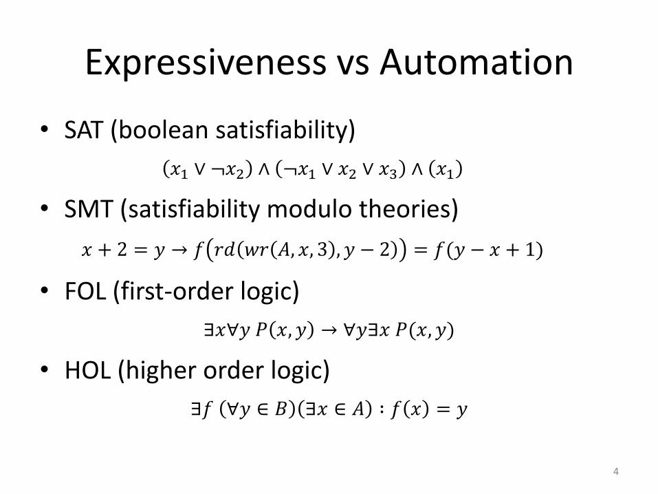
Expressiveness vs Automation

• SAT (boolean satisfiability)

𝑥1 ∨ ¬𝑥2 ∧ ¬𝑥1 ∨ 𝑥2 ∨ 𝑥3 ∧ 𝑥1

• SMT (satisfiability modulo theories)

𝑥 + 2 = 𝑦 → 𝑓 𝑟𝑑 𝑤𝑟 𝐴, 𝑥, 3 , 𝑦 − 2 = 𝑓(𝑦 − 𝑥 + 1)

• FOL (first-order logic)

∃𝑥∀𝑦 𝑃 𝑥, 𝑦 → ∀𝑦∃𝑥 𝑃(𝑥, 𝑦)

• HOL (higher order logic)

∃𝑓 ∀𝑦 ∈ 𝐵 ∃𝑥 ∈ 𝐴 ∶ 𝑓 𝑥 = 𝑦

4

Applications and Success Stories

• Proof of Robbins conjecture using theorem proverEQP (1996)

• Design and verification of Intel Core i7 processor using SAT technology (2009)

• Certified Windows 7 device drivers using SMT (2010)

• Flyspeck project: formal proof of the KeplerConjecture using Isabelle and HOL Light proof assistants (2014)

• . . .

5

Theorem Prover =

input clauses

6

Inference System + Search Algorithm

1. pick clause

2. find candidates

3. perform inferences

P(X) ∨ Q(X)

search space

¬P(a)

Q(a)

Theorem Prover =

7

input clauses

Inference System + Search Algorithm

false1. pick clause

2. find candidates

3. perform inferences

search space

Theorem Prover =

8

Inference System + Search Algorithm

Memory

Time

Demo (Vampire theorem prover)

• Group theory: if a group satisfies the identity 𝑥2 = 1, then it is commutative.

• Set theory: ∪ is commutative.

∀𝑥 ∶ 1 ⋅ 𝑥 = 𝑥

Axioms of group theory ∀𝑥 ∶ 𝑥−1 ⋅ 𝑥 = 𝑥

∀𝑥∀𝑦∀𝑧 ∶ 𝑥 ⋅ 𝑦 ⋅ 𝑧 = 𝑥 ⋅ 𝑦 ⋅ 𝑧

Assumption ∀𝑥 ∶ 𝑥 ⋅ 𝑥 = 1

Conjecture ∀𝑥∀𝑦 ∶ 𝑥 ⋅ 𝑦 = 𝑦 ⋅ 𝑥

Axioms of set theory∀𝐴∀𝐵∀𝑥 ∶ 𝑥 ∈ 𝐴 ∪ 𝐵 ↔ 𝑥 ∈ 𝐴 ∨ 𝑥 ∈ 𝐵

∀𝐴∀𝐵 ∶ ∀𝑥 ∶ 𝑥 ∈ 𝐴 ↔ 𝑥 ∈ 𝐵 → 𝐴 = 𝐵

Conjecture ∀𝐴∀𝐵 ∶ 𝐴 ∪ 𝐵 = 𝐵 ∪ 𝐴

9

Options in Vampireage_weight_ratioaig_bdd_sweepingaig_conditional_rewritingaig_definition_introductionaig_definition_introduction_thresholdaig_formula_sharingaig_inlinerarity_checkbackward_demodulationbackward_subsumptionbackward_subsumption_resolutionbfntbinary_resolutionbp_add_collapsing_inequalitiesbp_allowed_fm_balancebp_almost_half_bounding_removalbp_assignment_selectorbp_bound_improvement_limitbp_conflict_selectorbp_conservative_assignment_selectionbp_fm_eliminationbp_max_prop_lengthbp_propagate_after_conflictbp_start_with_precisebp_start_with_rationalbp_variable_selectorcolor_unblockingcondensationdecodedemodulation_redundancy_checkdistinct_processorepr_preserving_namingepr_preserving_skolemizationepr_restoring_inliningequality_propagationequality_proxyequality_resolution_with_deletionextensionality_allow_pos_eqextensionality_max_lengthextensionality_resolutionflatten_top_level_conjunctionsforbidden_optionsforced_optionsforward_demodulationforward_literal_rewriting

forward_subsumptionforward_subsumption_resolutionfunction_definition_eliminationfunction_numbergeneral_splittingglobal_subsumptionhorn_revealinghyper_superpositionignore_missingincludeincreased_numeral_weightinequality_splittinginput_fileinput_syntaxinst_gen_big_restart_ratioinst_gen_inprocessinginst_gen_passive_reactivationinst_gen_resolution_ratioinst_gen_restart_periodinst_gen_restart_period_quotientinst_gen_selectioninst_gen_with_resolutioninterpreted_simplificationlatex_outputlingva_additional_invariantsliteral_comparison_modelog_filelrs_first_time_checklrs_weight_limit_onlymax_activemax_answersmax_inference_depthmax_passivemax_weightmemory_limitmodename_prefixnamingniceness_optionnongoal_weight_coefficientnonliterals_in_clause_weightnormalizeoutput_axiom_namespredicate_definition_inliningpredicate_definition_merging

predicate_equivalence_discoverypredicate_equivalence_discovery_add_implicationspredicate_equivalence_discovery_random_simulationpredicate_equivalence_discovery_sat_conflict_limitpredicate_index_introductionprint_clausifier_premisesproblem_nameproofproof_checkingprotected_prefixquestion_answeringrandom_seedrow_variable_max_lengthsat_clause_activity_decaysat_clause_disposersat_learnt_minimizationsat_learnt_subsumption_resolutionsat_lingeling_incrementalsat_lingeling_similar_modelssat_restart_fixed_countsat_restart_geometric_increasesat_restart_geometric_initsat_restart_luby_factorsat_restart_minisat_increasesat_restart_minisat_initsat_restart_strategysat_solversat_var_activity_decaysat_var_selectorsaturation_algorithmselectionshow_activeshow_blockedshow_definitionsshow_interpolantshow_newshow_new_propositionalshow_nonconstant_skolem_function_traceshow_optionsshow_passiveshow_preprocessingshow_skolemisations

show_symbol_eliminationshow_theory_axiomssimulated_time_limitsine_depthsine_generality_thresholdsine_selectionsine_tolerancesmtlib_consider_ints_realsmtlib_flet_as_definitionsmtlib_introduce_aig_namessossplit_at_activationsplittingssplitting_add_complementaryssplitting_component_sweepingssplitting_congruence_closuressplitting_eager_removalssplitting_flush_periodssplitting_flush_quotientssplitting_nonsplittable_componentsstatisticssuperposition_from_variablessymbol_precedencetabulation_bw_rule_subsumption_resolution_by_lemmastabulation_fw_rule_subsumption_resolution_by_lemmastabulation_goal_awrtabulation_goal_lemma_ratiotabulation_instantiate_producing_rulestabulation_lemma_awrtest_idthankstheory_axiomstime_limittime_statisticstrivial_predicate_removalunit_resulting_resolutionunused_predicate_definition_removaluse_dismatchingweight_incrementwhile_numberxml_output

10

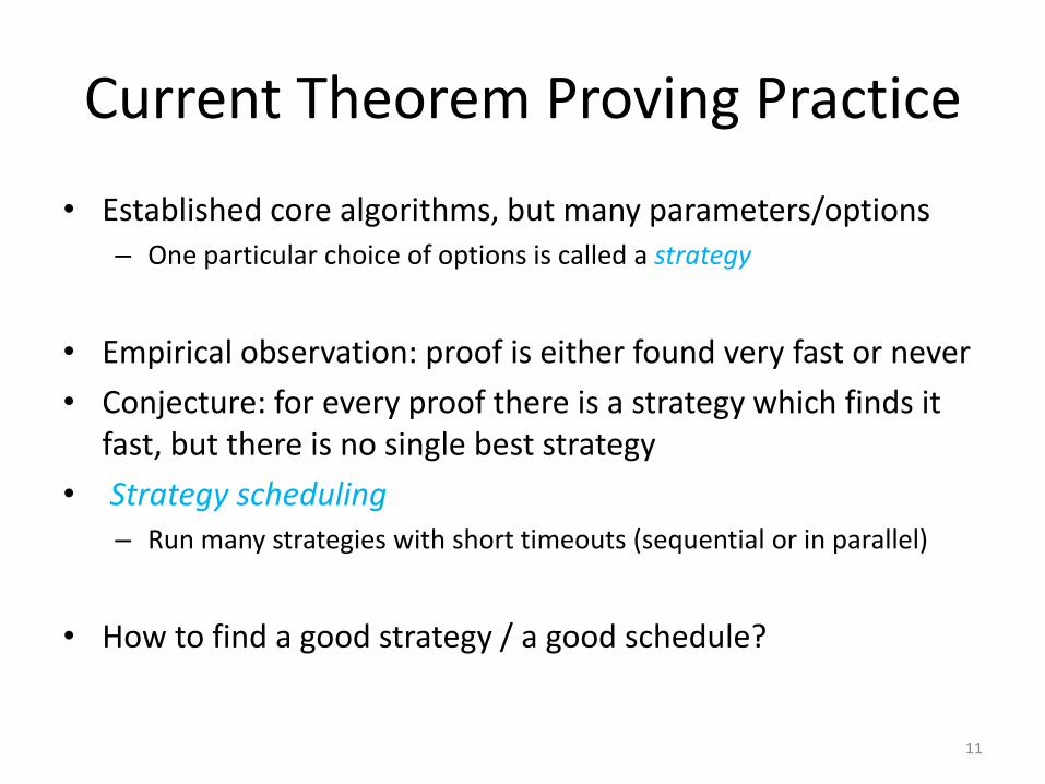
Current Theorem Proving Practice

• Established core algorithms, but many parameters/options– One particular choice of options is called a strategy

• Empirical observation: proof is either found very fast or never

• Conjecture: for every proof there is a strategy which finds it fast, but there is no single best strategy

• Strategy scheduling– Run many strategies with short timeouts (sequential or in parallel)

• How to find a good strategy / a good schedule?

11

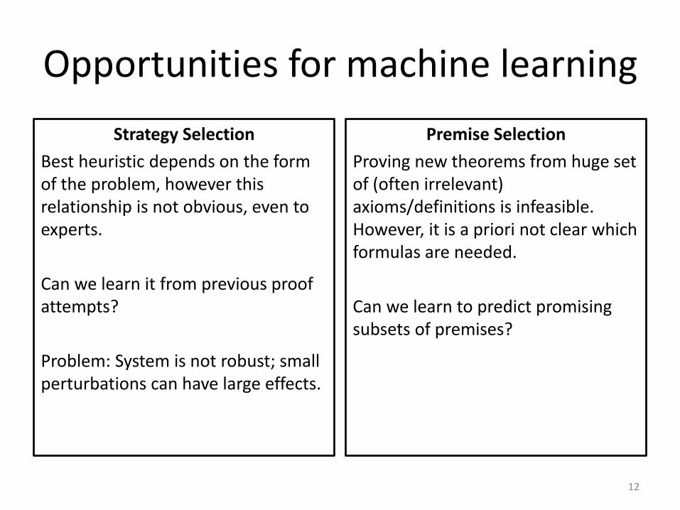
Opportunities for machine learning

Strategy Selection

Best heuristic depends on the form of the problem, however this relationship is not obvious, even to experts.

Can we learn it from previous proof attempts?

Problem: System is not robust; small perturbations can have large effects.

Premise Selection

Proving new theorems from huge set of (often irrelevant) axioms/definitions is infeasible. However, it is a priori not clear which formulas are needed.

Can we learn to predict promising subsets of premises?

12

Data Sets

Many existing benchmark libraries, e.g.:

• TPTP (Thousands of Problems for Theorem Provers) library

• Archive of Formal Proofs

• Mizar Mathematical Library

• SATLIB

• SMT-LIB

13

Interlude: Model Selection

1. Fit model(s) on training set

2. Choose best model / parameters on validation set

3. Report performance on test set

14

Test

Validation

Training

Data Set

Interlude: Model Selection

15

Instance-based learning (IBL)Suitability-value (SV)

[Fuchs, Automatic Selection Of Search-Guiding Heuristics For Theorem Proving, 1998]

16

Notation

• 𝒮 = {𝑠1, … , 𝑠𝑚} set of strategies

• 𝒫 = {𝑝1, … , 𝑝𝑛} set of training/validation/test problems

• 𝜏(𝑝, 𝑠) runtime of strategy 𝑠 on problem 𝑝

• 𝑇 timeout for proof attempts

• 𝑓 𝑝 = 𝑓1 𝑝 ,… , 𝑓𝑘 𝑝 feature vector of problem 𝑝

if convenient, we only write 𝑝 to denote the feature vector

17

Setting

• Given a new problem 𝑝, find a schedule 𝑆 of strategies (i.e. a permutation 𝜎) to run in sequence on 𝑝.

𝑆 = 𝑠𝜎(1), … , 𝑠𝜎(𝑚)

• Let the 𝑖th strategy be the first in 𝑆 that succeeds on 𝑝𝜏 𝑝, 𝑆 = 𝑖 − 1 𝑇 + 𝜏(𝑝, 𝑠𝜎 𝑖 )

• Reference schedules:

– 𝑆𝑜𝑝𝑡(𝑝) best strategy for 𝑝 at first position

– 𝑆𝑓𝑖𝑥 fixed schedule such that 𝑝∈𝒫 𝜏(𝑝, 𝑆𝑓𝑖𝑥) is smallest

• Euclidean distance between two problems 𝑝 and 𝑝′

𝛿 𝑝, 𝑝′ = 𝑖=1

𝑘

𝑓𝑖 𝑝 − 𝑓𝑖 𝑝′ 2

18

IBL-based Approach

• Pair each training problem 𝑝𝑖 with its best strategy 𝑠𝑖∗

• Let 𝑑𝑖 = 𝛿(𝑝, 𝑝𝑖) be the distance between 𝑝 and every training problem 𝑝𝑖

• Find 𝑑𝜋(1) ≤ ⋯ ≤ 𝑑𝜋(𝑛)

• Define 𝑆𝐼𝐵𝐿(𝑝) to be 𝑠𝜋(1)∗ , … , 𝑠𝜋(𝑛)

∗ with duplicates removed

and remaining strategies appended deterministically

• 𝑆𝐼𝐵𝐿∗ (𝑝): break distance ties by position in 𝑆𝑓𝑖𝑥

19

SV-based Approach

• Drawback of IBL: only closest neighbor is taken into account

• Compute suitability value 𝑣𝑗 for every strategy 𝑠𝑗

𝑣𝑗 = 𝑖=1

𝑛

Ψ 𝑑𝑖 , 𝜏 𝑝𝑖 , 𝑠𝑗

Ψ𝑒 𝑑, 𝑡 =

𝑇

𝑑+1 𝑒 , 𝑡 = ∞

𝑡

𝑑+1 𝑒 , else; 𝑒 ∈ ℕ, 𝑇 ≥ 𝑇

• Find 𝑣𝜋(1) ≤ ⋯ ≤ 𝑣𝜋(𝑚) and set 𝑆𝑆𝑉 𝑝 = 𝑠𝜋 1 , … , 𝑠𝜋(𝑚)

• Penalize timeout by the number of other strategies that also timeout 𝑆𝑆𝑉

∗ 𝑝 𝑇

𝑑 + 1 𝑒 ⋅ | 𝑠𝑙 𝜏 𝑝𝑖 , 𝑠𝑙 = ∞}|

20

Experimental Evaluation

• Discount theorem prover with 𝑚 = 5 strategies

• 263 equational problems from six TPTP categories

• Timeout 𝑇 = 600s

• Features

• Parameters 𝑒 = 4 and 𝑇 = 1000s

21

Experimental Evaluation

22

training data = test data

Robustness ratio

𝑟𝑓𝑖𝑥 ≈ 0.71 𝑟𝑋 > 0.99 for 𝑋 ≠ 𝑓𝑖𝑥

Experimental Evaluation

23

90% training data

Support Vector Machines

[Bridge, Machine Learning and Automated Theorem Proving, 2010]

[Bridge et al., Machine Learning for First-Order Theorem Proving, 2014]

24

Setting

• 6118 sample problems 𝒫 from the TPTP library

• Theorem prover E with five preselected strategies 𝒮

• From runtimes 𝜏(𝑝, 𝑠) (100s timeout) build data set for every strategy 𝑠𝑖

𝒟𝑖 = 𝑓 𝑝1 , 𝑦1𝑖

, … , 𝑓 𝑝𝑛 , 𝑦𝑛𝑖

𝑦𝑗𝑖

= +1/−1, depending on whether

𝑠𝑖 was fastest strategy on 𝑝𝑗 or not

• Special strategy 𝑠0 and data set 𝒟0 denoting rejection of “too hard” problems

• Goal: given problem 𝑝, predict best strategy to find proof within 100s

25

…..

Features

26

14 static features 39 dynamic features

Performance Measures

For a validation/test set of size 𝑚, define𝑃+/𝑃− # true/false positives

𝑁+/𝑁− # true/false negatives

• Accuracy: 𝑎𝑐𝑐 =𝑃++𝑁+

m

• Matthews correlation coefficient: M =𝑃+𝑁+−𝑃−𝑁−

(P++P−)(P++N−)(N++P−)(N++N−)

1…perfect prediction 0…like random classifier -1…opposite to data

• F1 score: F1 =2𝑝𝑟

p+r∈ 0,1

precision 𝑝 = 𝑃+/(𝑃+ + 𝑃−) recall 𝑟 = 𝑃+/(𝑃+ + 𝑁−)

27

Support Vector Machinein Kernelized Form

• Classifier for sample 𝒙 is given by

sign

𝑖

𝛼𝑖𝑘 𝒙𝑖 , 𝒙 + 𝑏

• Regularization parameter 𝐶 controls trade-off between robustness and correctness– can be split into 𝐶+ and 𝐶− to give different weights for positive and

negative samples ratio parameter 𝑗

𝑗 =𝐶+

𝐶− =# positive samples

# negative samples

• Kernels

28

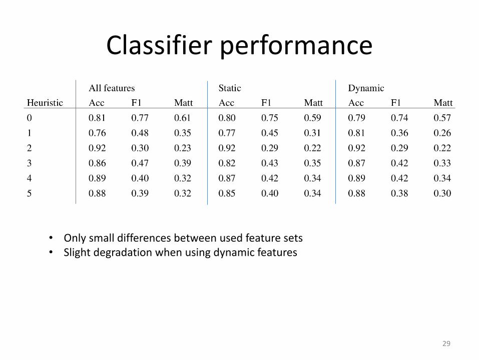
Classifier performance

29

• Only small differences between used feature sets• Slight degradation when using dynamic features

Combining Classifiersfor Heuristic Selection

30

Interpret value of classifier (before applying sign) as confidence in labeling input +1 Select strategy with largest value

• Learned strategies outperform every fixed strategy• Performance with dynamic features is worse• Allowing the rejection of problems reduces runtime drastically

Feature selection

• Usually applied to reduce huge feature sets to make learning feasible

• Here: provide useful information for strategy development

• Techniques:– Filter approach

– Embedded approach

– Wrapper approach

• Exhaustive test of all feature subsets up to size 3 similar results can be obtained with only a few features

31

MaLeS - Machine Learning of Strategies

[Kühlwein et al., MaLeS: A Framework for Automatic Tuning of Automated Theorem Provers, 2013]

[Kühlwein, Machine Learning for Automated Reasoning, 2014]

32

MaLeS

• Parameter tuning framework– Automatically find set 𝒮 of preselected strategies

– Construct individual strategy schedule for new problems

• Learned object: runtime prediction functions𝜌𝑠 ∶ 𝒫 → ℝ

– Kernel method

– Only learn on problems that can be solved within timeout

– Update of prediction function during runtime

33

Finding good search strategies

34

Stochastic local search algorithm

E-MaLeS strategy search:• 1112 problems• Three weeks on 64 core server• 109 strategies selected,

out of 2 million

Features

35

Again absolute values, instead of ratios.

Learning the prediction function

• Prediction function has the form

𝜌𝑠 𝑝 = 𝑝′∈𝒫 𝛼𝑝′𝑠 𝑘 𝑝, 𝑝′ for some 𝛼𝑝′

𝑠 ∈ ℝ

• Kernel matrix 𝐾𝑠 ∈ ℝ𝑚×𝑚 is 𝐾𝑖,𝑗𝑠 = 𝑘(𝑝𝑖 , 𝑝𝑗)

• Time matrix 𝑌𝑠 ∈ ℝ1×𝑚 is 𝑌𝑖𝑠 = 𝜏(𝑝𝑖 , 𝑠)

• Weight matrix 𝐴𝑠 ∈ ℝ𝑚×1 is 𝐴𝑖𝑠 = 𝛼𝑝𝑖

𝑠

• Least square regression𝐴 = argmin

𝐴∈ℝ𝑚×1( 𝑌 − 𝐾𝐴 𝑇 𝑇 − 𝐾𝐴 + 𝐶𝐴𝑇𝐾𝐴)

• Theorem𝐴 = 𝐾 + 𝐶𝐼 −1𝑌

36

• Delete training problems that are solved by the picked strategy within the predicted runtime

• Retrain prediction function

Creating Schedulesfrom Prediction Functions

37

Evaluation

38

Conclusion

• Existing case studies showed applicability of machine learning techniques to strategy selection in theorem provers– Nearest neighbor

– Similarity value

– Support vector machines

• Requires many decisions different settings

• Results often inconclusive

• Not yet a direct benefit for developers or users

39