Machine Learning: Exercise Sheet 2

Machine Learning: Exercise Sheet 2

Manuel BlumAG Maschinelles Lernen und Naturlichsprachliche Systeme

Albert-Ludwigs-Universitat Freiburg

[email protected]

Manuel Blum Machine Learning Lab, University of Freiburg Machine Learning: Exercise Sheet 2 (1)

Exercise 1: Version SpacesTask (a)

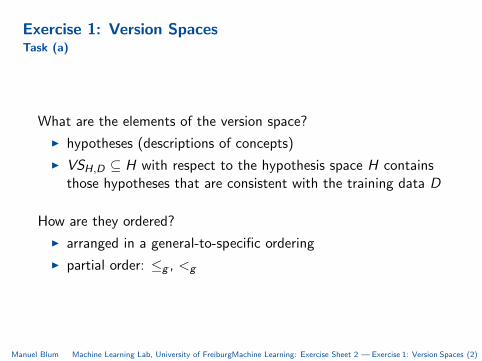
What are the elements of the version space?

I hypotheses (descriptions of concepts)

I VSH,D ⊆ H with respect to the hypothesis space H containsthose hypotheses that are consistent with the training data D

How are they ordered?

I arranged in a general-to-specific ordering

I partial order: ≤g , <g

Manuel Blum Machine Learning Lab, University of FreiburgMachine Learning: Exercise Sheet 2 — Exercise 1: Version Spaces (2)

Exercise 1: Version SpacesTask (a)

What can be said about the meaning and sizes of G and S?

I They are sets containing the most general and most specifichypotheses consistent with the training data. Thus, theydepict the general and specific boundary of the VS.

I For conjunctive hypotheses (which we consider here) it alwaysholds |S | = 1, assuming consistent training data. G attains itsmaximal size, if negative patterns with maximal hammingdistance have been presented. Thus, in the case of binaryconstraints, it holds |G | ≤ n(n − 1) where n denotes thenumber of constraints per hypothesis.


Exercise 1: Version SpacesTask (b)

In the following, it is desired to describe whether a person is ill.We use a representation based on conjunctive constraints (threeper subject) to describe individual person. These constraints are“running nose”, “coughing”, and “reddened skin”, each of whichcan take the value true (‘+’) or false (‘–’). We say that somebodyis ill, if he is coughing and has a reddened nose — each singlesymptom individually does not mean that the person is ill.

I Specify the space of hypotheses that is being managed by theversion space approach. To do so, arrange all hypotheses in agraph structure using the more-specific-than relation.

I hypotheses are vectors of constraints, denoted by 〈N,C ,R〉I with N,C ,R = {−,+, ∅, ∗}


Exercise 1: Version SpacesTask (c)

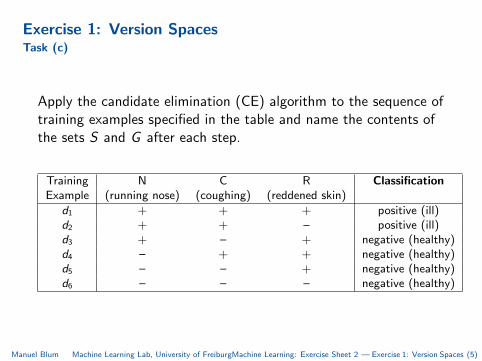
Apply the candidate elimination (CE) algorithm to the sequence oftraining examples specified in the table and name the contents ofthe sets S and G after each step.

Training N C R ClassificationExample (running nose) (coughing) (reddened skin)

d1 + + + positive (ill)d2 + + – positive (ill)d3 + – + negative (healthy)d4 – + + negative (healthy)d5 – – + negative (healthy)d6 – – – negative (healthy)



I Start (init): G = {〈∗ ∗ ∗〉}, S = {〈∅∅∅〉}I foreach d ∈ D do

I d1 = [〈+ + +〉, pos]⇒ G = {〈∗ ∗ ∗〉}, S = {〈+ + +〉}I d2 = [〈+ +−〉, pos]⇒ G = {〈∗ ∗ ∗〉}, S = {〈+ + ∗〉}I d3 = [〈+−+〉, neg ]

I no change to S : S = {〈+ + ∗〉}I specializations of G : G = {〈− ∗ ∗〉, 〈∗+ ∗〉, 〈∗ ∗ −〉}I there is no element in S that is more specific than the first

and third element of G→ remove them from G ⇒ G = {〈∗+ ∗〉}



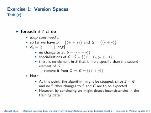
I foreach d ∈ D doI loop continued ...I so far we have S = {〈+ + ∗〉} and G = {〈∗+ ∗〉}I d4 = [〈−+ +〉, neg ]

I no change to S : S = {〈+ + ∗〉}I specializations of G : G = {〈+ + ∗〉, 〈∗+−〉}I there is no element in S that is more specific than the second

element of G→ remove it from G ⇒ G = {〈+ + ∗〉}

I Note:I At this point, the algorithm might be stopped, since S = G

and no further changes to S and G are to be expected.I However, by continuing we might detect inconsistencies in the

training data.



I Start (init): G = {〈∗ ∗ ∗〉}, S = {〈∅∅∅〉}I foreach d ∈ D do

I loop continued ...I d5 = [〈− −+〉, neg ] ⇒ Both, G = {〈+ + ∗〉} and

S = {〈+ + ∗〉} are consistent with d5.I d6 = [〈− − −〉, neg ] ⇒ Both, G = {〈+ + ∗〉} and

S = {〈+ + ∗〉} are consistent with d6.

I return S and G


Exercise 1: Version SpacesTask (d)

Does the order of presentation of the training examples to thelearner affect the finally learned hypothesis?

I No, but it may influence the algorithm’s running time.


Exercise 1: Version SpacesTask (e)

Assume a domain with two attributes, i.e. any instance is describedby two constraints. How many positive and negative trainingexamples are minimally required by the candidate eliminationalgorithm in order to learn an arbitrary concept?

I By learning an arbitrary concept, of course, we mean that thealgorithm arrives at S = G .

I The algorithm is started with S = {〈∅, ∅〉} and G = {〈∗, ∗〉}.I We just consider the best cases, i.e. situations in where the

training instances given to the CE algorithm allow foradapting S or G .


Exercise 1: Version SpacesTask (e)

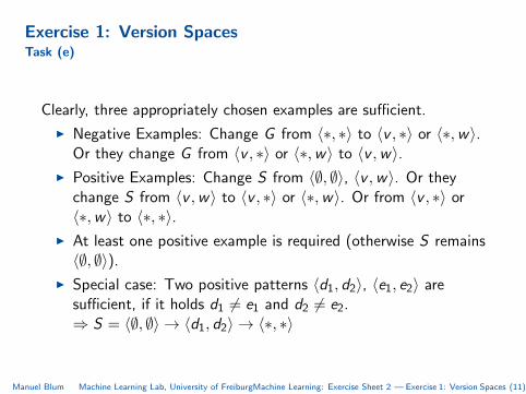
Clearly, three appropriately chosen examples are sufficient.

I Negative Examples: Change G from 〈∗, ∗〉 to 〈v , ∗〉 or 〈∗,w〉.Or they change G from 〈v , ∗〉 or 〈∗,w〉 to 〈v ,w〉.

I Positive Examples: Change S from 〈∅, ∅〉, 〈v ,w〉. Or theychange S from 〈v ,w〉 to 〈v , ∗〉 or 〈∗,w〉. Or from 〈v , ∗〉 or〈∗,w〉 to 〈∗, ∗〉.

I At least one positive example is required (otherwise S remains〈∅, ∅〉).

I Special case: Two positive patterns 〈d1, d2〉, 〈e1, e2〉 aresufficient, if it holds d1 6= e1 and d2 6= e2.⇒ S = 〈∅, ∅〉 → 〈d1, d2〉 → 〈∗, ∗〉


Exercise 1: Version SpacesTask (f)

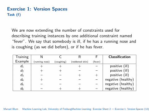
We are now extending the number of constraints used fordescribing training instances by one additional constraint named“fever”. We say that somebody is ill, if he has a running nose andis coughing (as we did before), or if he has fever.

Training N C R F ClassificationExample (running nose) (coughing) (reddened skin) (fever)

d1 + + + – positive (ill)d2 + + – – positive (ill)d3 – – + + positive (ill)d4 + – – – negative (healthy)d5 – – – – negative (healthy)d6 – + + – negative (healthy)



How does the version space approach using the CE algorithmperform now, given the training examples specified on the previousslide?

I Initially: S = {〈∅∅∅∅〉}, G = {〈∗ ∗ ∗∗〉}I d1 = [〈+ + +−〉, pos] ⇒ S = {〈+ + +−〉}, G = {〈∗ ∗ ∗∗〉}I d2 = [〈+ +−−〉, pos] ⇒ S = {〈+ + ∗−〉}, G = {〈∗ ∗ ∗∗〉}I d3 = [〈− −++〉, pos] ⇒ S = {〈∗ ∗ ∗∗〉}, G = {〈∗ ∗ ∗∗〉}→ We already arrive at S = G .

I d4 = [〈+−−−〉, neg ] ⇒ S = {〈∗ ∗ ∗∗〉}, G = {〈∗ ∗ ∗∗〉}I Now, S becomes empty since 〈∗ ∗ ∗∗〉 is inconsistent with d4

and is removed from S .I G would be specialized to{〈− ∗ ∗∗〉, 〈∗+ ∗∗〉, 〈∗ ∗+∗〉, 〈∗ ∗ ∗+〉}. But it is required thatat least one element from S must be more specific than anyelement from G .→ This requirement cannot be fulfilled since S = ∅. ⇒ G = ∅



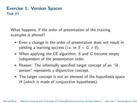
What happens, if the order of presentation of the trainingexamples is altered?

I Even a change in the order of presentation does not result inyielding a learning success (i.e. in S = G 6= ∅).

I When applying the CE algorithm, S and G become emptyindependent of the presentation order.

I Reason: The informally specified target concept of an “illperson” represents a disjunctive concept.

I The target concept is not an element of the hypothesis spaceH (which is made of conjunctive hypotheses).


Exercise 2: Decision Tree Learning with ID3Task (a)

Apply the ID3 algorithm to the training data in the table.

Training fever vomiting diarrhea shivering Classificationd1 no no no no healthy (H)d2 average no no no influenza (I)d3 high no no yes influenza (I)d4 high yes yes no salmonella poisoning (S)d5 average no yes no salmonella poisoning (S)d6 no yes yes no bowel inflammation (B)d7 average yes yes no bowel inflammation (B)

Manuel Blum Machine Learning Lab, University of Freiburg Machine Learning: Exercise Sheet 2 — Exercise 2: ID3 (15)


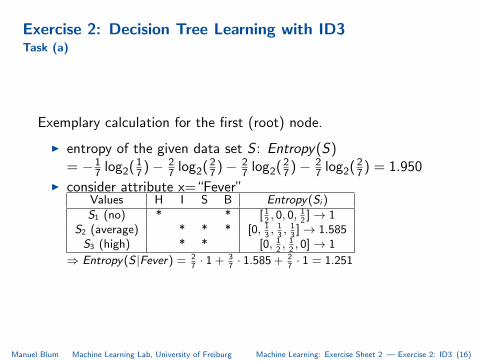
Exemplary calculation for the first (root) node.

I entropy of the given data set S : Entropy(S)= −1

7 log2(17)− 27 log2(27)− 2

7 log2(27)− 27 log2(27) = 1.950

I consider attribute x=“Fever”Values H I S B Entropy(Si )

S1 (no) * * [ 12, 0, 0, 1

2]→ 1

S2 (average) * * * [0, 13, 13, 13]→ 1.585

S3 (high) * * [0, 12, 12, 0]→ 1

⇒ Entropy(S |Fever) = 27· 1 + 3

7· 1.585 + 2

7· 1 = 1.251



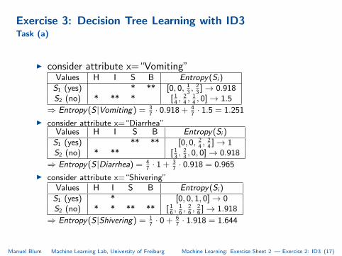
I consider attribute x=“Vomiting”Values H I S B Entropy(Si )

S1 (yes) * ** [0, 0, 13, 23]→ 0.918

S2 (no) * ** * [ 14, 24, 14, 0]→ 1.5

⇒ Entropy(S |Vomiting) = 37· 0.918 + 4

7· 1.5 = 1.251

I consider attribute x=“Diarrhea”Values H I S B Entropy(Si )

S1 (yes) ** ** [0, 0, 24, 24]→ 1

S2 (no) * ** [ 13, 23, 0, 0]→ 0.918

⇒ Entropy(S |Diarrhea) = 47· 1 + 3

7· 0.918 = 0.965

I consider attribute x=“Shivering”Values H I S B Entropy(Si )

S1 (yes) * [0, 0, 1, 0]→ 0S2 (no) * * ** ** [ 1

6, 16, 26, 26]→ 1.918

⇒ Entropy(S |Shivering) = 17· 0 + 6

7· 1.918 = 1.644



choose the attribute that maximizes the information gain

I Fever: Gain(S) = Ent(S)− Ent(S |Fever) = 1.95− 1.251 = 0.699

I Vomiting: Gain(S) = Ent(S)− Ent(S|Vomit) = 1.95− 1.251 = 0.699

I Diarrhea: Gain(S) = Ent(S)− Ent(S|Diarrh) = 1.95− 0.965 = 0.985

I Shivering: Gain(S) = Ent(S)− Ent(S |Shiver) = 1.95− 1.644 = 0.306

⇒ Attribute “Diarrhea” is the most effective one,maximizing the information gain.


Exercise 3: Decision Tree Learning with ID3Task (b)

Does the resulting decision tree provide a disjoint definition of theclasses?

I Yes, the resulting decision tree providesdisjoint class definitions.


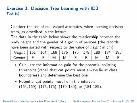
Exercise 3: Decision Tree Learning with ID3Task (c)

Consider the use of real-valued attributes, when learning decisiontrees, as described in the lecture.The data in the table below shows the relationship between thebody height and the gender of a group of persons (the recordshave been sorted with respect to the value of height in cm).Height 161 164 169 175 176 179 180 184 185

Gender F F M M F F M M F

I Calculate the information gain for the potential splittingthresholds (recall that cut points must always lie at classboundaries) and determine the best one.

I Potential cut points must lie in the intervals(164, 169), (175, 176), (179, 180), or (184, 185).



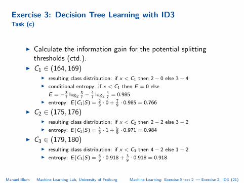
I Calculate the information gain for the potential splittingthresholds (ctd.).

I C1 ∈ (164, 169)I resulting class distribution: if x < C1 then 2− 0 else 3− 4

I conditional entropy: if x < C1 then E = 0 else

E = − 37log2

37− 4

7log2

47= 0.985

I entropy: E(C1|S) = 29· 0 + 7

9· 0.985 = 0.766


I entropy: E(C2|S) = 49· 1 + 5

9· 0.971 = 0.984


I entropy: E(C3|S) = 69· 0.918 + 3

9· 0.918 = 0.918



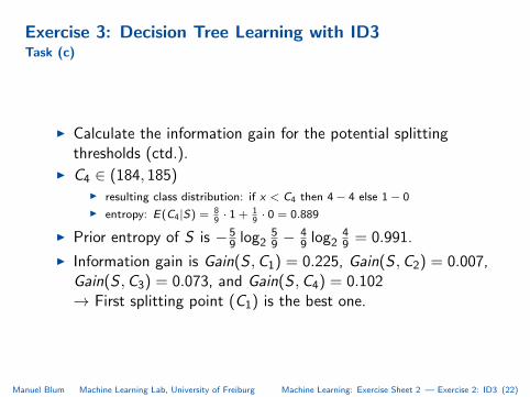
I Calculate the information gain for the potential splittingthresholds (ctd.).


I entropy: E(C4|S) = 89· 1 + 1

9· 0 = 0.889

I Prior entropy of S is −59 log2

59 −

49 log2

49 = 0.991.

I Information gain is Gain(S ,C1) = 0.225, Gain(S ,C2) = 0.007,Gain(S ,C3) = 0.073, and Gain(S ,C4) = 0.102→ First splitting point (C1) is the best one.


Machine Learning: Exercise Sheet 2

Documents

Transcript of Machine Learning: Exercise Sheet 2