
WE4.L09 - ROLL INVARIANT TARGET DETECTION BASED ON POLSAR CLUTTER MODELS

Machine Learning Based Regression Model for Forest
Aboveground Biomass Estimation using RISAT-1 PolSAR and TLS
Lidar Data
Thesis submitted to the Andhra University, Visakhapatnam
in partial fulfilment of the requirement for the award of
Master of Technology in Remote Sensing and GIS
Submitted By Rohit Mangla
Supervised By
Mr. Shashi Kumar
Scientist/Engineer ‘SD’
Photogrammetry & Remote Sensing
Department
Indian Institute of Remote Sensing
Dehradun
Dr. Subrata Nandy
Scientist/Engineer ‘SD’
Forestry & Ecology
Department
Indian Institute of Remote Sensing
Dehradun
Indian Institute of Remote Sensing,
Indian Space Research Organization,
Department of Space, Govt. of India
Dehradun – 248001
Uttarakhand, India
August, 2015

i
DISCLAIMER
This work has been carried out in partial fulfillment of Masters of Technology program in
Remote Sensing and Geographic Information System at Indian Institute of Remote Sensing,
Dehradun, India. The author is solely responsible for the contents of the thesis

ii
ACKNOWLEDGEMENT
I would like to thank my parents for their love, affection, belief and faith in my capability.
Then I would like to thank my supervisor Mr. Shashi Kumar for supporting and guiding me
throughout the year. He has taught me like a teacher, supported me like a parent and guided
me like a supervisor. His direction have brought me to the completion of this thesis. I would
also thank my co-supervisor Dr. Subrata Nandy Sir who taught me forestry terms and made
it easy for me. He gave me the freedom to do mistakes and learn from them. His patience and
care in supporting me are invaluable. The guidance & strategy of my guides for this work are
highly appreciable.
I would like to express my deepest gratitude to Dr. Y.V.N. Krishna Murthy, former Director
IIRS, and Dr. A. Senthil Kumar, Director IIRS for providing all the opportunities and facilities
that was required for the successful execution of the project. I would like to thanks to my
guide as a HOD & course director of M.Tech course Ms. Shefali Agrawal for her concern on
us and efficient management of academic activities that helped us complete our course
curriculum with ease and in time.
I sincerely express my gratitude to Akshat, Rigved, Varun, Manohar, Ridhika, Richa, Jenia,
Rajasweta Datta and Mayank sir in the PRSD lab who were always a team and created the
best working environment in all possible ways. I would like to thank to Neeraj, Kildar and
Amol for their support in my field work.
I would also like to thank to my friends Sukant, Kuldip Sir, Rajkumar Ji, Harjeet Paji, Vineet,
Utsav, and Reshma for making my life so very easy by their constant company. A special
thanks to Mr. Rahul (CMA) for helping me out in my project whenever I was struck with
some server or data problems.
I also thanks to my cousin sister, Ayushi Goyal and cousin brother Dr. Saurabh Goyal for
their encouragement.
Rohit Mangla
M.Tech 2013-2015

iii
CERTIFICATE
This is to certify that the project entitled “Machine Learning Based Regression Model for
Forest Aboveground Biomass Estimation using RISAT-1 PolSAR and TLS Lidar Data”
is a bonafide record of work carried out by Mr. Rohit Mangla during 01 Aug 2014 to 14 Aug
2015. The report has been submitted in partial fulfillment of requirement for the award of
Master of Technology in Remote Sensing and GIS with specialization in Satellite Image
Analysis and Photogrammetry, conducted at Indian Institute of Remote Sensing (IIRS),
Indian Space Research Organisation (ISRO), Dehradun from 19 Aug 2013 to 14 Aug 2015.
The work has been carried out under the supervision of Mr. Shashi Kumar,
Scientist/Engineer ‘SD’, Photogrammetry and Remote Sensing Department and Dr.
Subrata Nandy, Scientist/Engineer ‘SD’, Forestry and Ecology Department.
No part of this report is to be published without the prior permission/intimation from/to the
undersigned.
Mr. Shashi Kumar
Scientist/Engineer ‘SD’
Photogrammetry and Remote
Sensing Department
IIRS, Dehradun
Dr. Subrata Nandy
Scientist/Engineer ‘SD’
Forestry and Ecology
Department
IIRS, Dehradun
Ms. Shefali Agrawal
Scientist/Engineer ‘SG’ and Head
Photogrammetry and Remote
Sensing Department
IIRS, Dehradun
Dr. S.P.S. Kushwaha
Dean, Academics & Group
Director ERSSG
IIRS, Dehradun

iv
DECLARATION
I, Rohit Mangla, hereby declare that this dissertation entitled “Machine Learning Based
Regression Model for Forest Aboveground Biomass Estimation using RISAT-1 PolSAR
and TLS Lidar Data” submitted to Andhra University, Visakhapatnam in partial fulfilment
of the requirements for the award of M.Tech in Remote Sensing and GIS, is my own work
and that to the best of my knowledge and belief. It is a record of original research carried out
be me under the guidance and supervision of Mr. Shashi Kumar, Scientist ‘SD’ and Dr.
Subrata Nandy, Scientist ‘SD’, Forestry and Ecology Department, Indian Institute of Remote
Sensing, ISRO, Dehradun. It contains no material previously published or written by another
person nor material which to a substantial extent nor material which to a substantial extent
has been accepted for the award of any other degree or diploma of the university or other
institute of higher learning, except where due acknowledgement has been made in the text.
Place: Dehradun Mr. Rohit Mangla
Date: Aug, 2015

v
Dedicated to my
beloved nana ji…

vi
ABSTRACT
Forest are the major source of carbon content and influences the carbon cycle. It is necessary
to assess aboveground biomass (AGB) to determine the health of forest, greenhouse effect
and climate change studies. Traditional based methods are laborious, time consuming,
expensive and accessible to limited areas. Remote Sensing and GIS based methods are very
effective in AGB assessment. The current research work has focused on SAR and Lidar
remote sensing methods. Because SAR has the capability of penetrating the cloud cover and
Lidar can capture the 3D information of the tree structure. A part of Timli forest range was
selected for the study. Here, RISAT-1 FRS2 quad pol data acquired in C band was utilized.
The three different decomposition models were used to extract the scattering variables and
the comparative study suggested to use multi-component and Yamaguchi models scattering
elements as input parameters for biomass modeling. Tree biophysical parameters like stem
diameter and tree height were extracted from terrestrial Lidar data. This study used the multi
scanning approach and removes the occlusion effects as suggested by previous studies. An
individual tree point cloud was digitized because of problem in handling the large amount of
data. From the single tree cloud, slicing of tree at a particular ground height was done and
least square algorithm was applied to estimate stem diameter. The results for stem diameter
(R2=0.85 and RMSE= 5.35 cm) was satisfactory. The z coordinates difference of the tree
ground position and peak point gives the tree height and it was validated with the field data
with correlation parameters (R2= 0.69 and RMSE= 2.325m). This work analyzed the two
modelling approach for AGB assessment. Multi-linear regression method used the SAR based
scattering variables while Random forest modelling approach used the SAR and Lidar
parameters as input variables. The results from random forest modelling approach (R2= 0.63
and RMSE=27.68 t/ha) was found better than multiple linear regression approach (R2= 0.5
and RMSE=12.58 t/ha). It was found that helix scattering shows negative correlation with
biomass and volume and surface scattering were highly correlated with each other. The results
concluded that the integration of Lidar and SAR variables improves the accuracy. Diameter
and volume scattering were the sensitive parameters for AGB assessment. This study also
suggested to do more research on other forest parameters like basal area and stem volume,
crown gap and density using terrestrial laser scanner data.
Keywords: Aboveground Biomass, RISAT-1, Decomposition models, Terrestrial Laser
Scanner, Least square Analysis, Multi-Linear Regression model, Random Forest Model

vii
Table of Contents ABSTRACT ........................................................................................................................... vi
List of Figures ........................................................................................................................ ix
List of Tables ......................................................................................................................... xi
Acronyms .............................................................................................................................. xii
1 Introduction ..................................................................................................................... 1
1.1 Background ............................................................................................................. 1
1.2 Microwave Remote Sensing ................................................................................... 1
1.3 Terrestrial Lidar Remote Sensing for tree biophysical parameters estimation ....... 2
1.4 Motivation and Problem Statement......................................................................... 3
1.5 Innovation ............................................................................................................... 4
1.6 Research objectives ................................................................................................. 4
1.6.1 Sub objectives ................................................................................................. 4
1.6.2 Research Questions ......................................................................................... 5
1.7 Structure of the thesis .............................................................................................. 5
2 Literature Review ............................................................................................................ 6
2.1 Biophysical parameters retrieval using optical datasets .......................................... 6
2.2 SAR Remote Sensing .............................................................................................. 6
2.2.1 Polarimetric Decomposition Modelling .......................................................... 7
2.2.2 Scattering Models ........................................................................................... 8
2.3 Three Dimensional Modelling of Forest Structure using Terrestrial laser scanner ..
.............................................................................................................................. 11
2.4 Modelling Approach for AGB Estimation ............................................................ 12
2.4.1 Semi-Empirical Model .................................................................................. 12
2.4.2 Machine learning based model ..................................................................... 13
2.4.3 Random Forest Regression Model ................................................................ 14
2.4.4 Decision Trees .............................................................................................. 14
3 Study Area and Materials .............................................................................................. 16
3.1 Study Area ............................................................................................................ 16
3.2 Materials ............................................................................................................... 17
3.2.1 Satellite Data ................................................................................................. 17
3.2.2 Terrestrial Laser Scanner .............................................................................. 17
3.2.3 In-situ Measurement ..................................................................................... 18
4 Methodology ................................................................................................................. 20
4.1 Radiometric Calibration ........................................................................................ 21
4.2 Multilooking ......................................................................................................... 22
4.3 Polarimetric Decomposition Modelling ................................................................ 23
4.3.1 Types of Decomposition Models .................................................................. 23
4.4 Feasibility Analysis of Polarimetric Decomposition Models ............................... 26
4.5 TLS Lidar data Processing .................................................................................... 26
4.5.1 TLS Data Acquisition ................................................................................... 26
4.5.2 Point Cloud Registration ............................................................................... 28
4.5.3 Individual Tree extraction ............................................................................. 30
4.6 Stem diameter Estimation using Least Square Circle Fit ...................................... 30

viii
4.6.1 Pratt’s Method for minimization ................................................................... 32
4.7 Modelling Approach for AGB Estimation ............................................................ 33
4.8 Multiple Linear Regression Modelling approach ................................................. 33
4.8.1 Regression model .......................................................................................... 34
4.9 Random Forest Regression modelling approach for AGB Estimation ................. 36
4.9.1 Random Forest Approach ............................................................................. 36
4.10 Validation (Accuracy Assessment) and sensitivity analysis ................................. 37
5 Result and Discussion ................................................................................................... 38
5.1 Radiometric Calibration of RISAT-1 data ............................................................ 38
5.2 Scattering Parameters retrieval using Polarimetric Decomposition Model .......... 39
5.3 Feasibility Analysis of Decomposition Models .................................................... 41
5.3.1 Comparative study of volume scattering retrieved from decomposition models
...................................................................................................................... 42
5.4 Terrestrial Lidar Data Results ............................................................................... 43
5.5 3D Visualization of an individual tree .................................................................. 44
5.6 Tree height Estimation and its validation ............................................................. 45
5.7 Stem Diameter Validation Curve (TLS Vs Field Diameter) ................................. 47
5.8 Multi linear Regression Results ............................................................................ 48
5.8.1 Regression Model 1 ...................................................................................... 48
5.8.2 Regression Model 2 ...................................................................................... 50
5.9 Random Forest Model Approach .......................................................................... 51
5.9.1 Decision tree construction using RISAT-1 derived Variables and field
Biomass ...................................................................................................................... 51
5.9.2 Variable importance (optimization) .............................................................. 53
5.10 Validation (multi-linear regression and Random Forest model) ........................... 54
5.11 Sensitivity Analysis of Input Variables ................................................................ 56
6 Conclusion and Recommendation ................................................................................ 57
6.1 Future Recommendation ....................................................................................... 58
References ............................................................................................................................. 59
Appendix 1 ............................................................................................................................ 67
Scan Parameters ................................................................................................................ 67
TLS Coordinate System .................................................................................................... 69
RISCAN PRO Results ...................................................................................................... 69
Appendix 2 ............................................................................................................................ 71
Van-Zyl Decomposition Model ........................................................................................ 71
Terrestrial Lidar Field Plots .............................................................................................. 73
Field Data .......................................................................................................................... 77
Field Photos ...................................................................................................................... 78
Research Publication

ix
List of Figures
Figure 2.1 A- double bounce scattering from the ground –trunk interaction, B- surface
scattering from the soil surface, C- volume scattering from the canopy, D- helix scattering
from the tree stem structures, E- wire scattering from the sharp edges of the canopy layer 10
Figure 2.2 Graphical view of Decision Tree ......................................................................... 15
Figure 3.1 Study Area ........................................................................................................... 16
Figure 3.2 Riegl VZ-400 Instrument (Carr, 2013) ................................................................ 18
Figure 3.3 Plot Sampling location in RISAT-1 Image .......................................................... 19
Figure 4.1 Methodology........................................................................................................ 20
Figure 4.2 RISAT-1 HH image (i) before calibration (ii) after calibration........................... 21
Figure 4.3 Shown the image before and after Multilooking ................................................. 22
Figure 4.4 Vanzyl decomposed results. Left side image is surface scattering, middle image is
double bounce scattering and last image is volume scattering ............................................. 23
Figure 4.5 Yamaguchi decomposition results. Starts from left image surface scattering, double
bounce scattering, volume scattering and helix scattering .................................................... 24
Figure 4.6 MCMS decomposition results. Start from the left image, surface scattering, double
bounce scattering, volume scattering, helix scattering and wire scattering .......................... 26
Figure 4.7 Geometry of sample plots .................................................................................... 27
Figure 4.8 Workflow of TLS Data Acquisition in multiple scanning ................................... 28
Figure 4.9 left side image shown the reflectance image of a sampled plot and right side image
display the point cloud after assigning the color intensity .................................................... 28
Figure 4.10 sampled plot scans captured from the different scan position and shadow was
appeared behind the trees due to occlusion effect ................................................................. 29
Figure 4.11 3D tree model generated after merged all scans. The disappear of shadow was
indicated that occlusion effect was removed ........................................................................ 29
Figure 4.12 (i) irregular tree structure (ii) Cylinder cross-section at z=1 plane.................... 30
Figure 4.13 show the correlation of each variable ................................................................ 34
Figure 4.14 Random Forest Approach .................................................................................. 37
Figure 5.1 Histogram plot with statistical parameters (i) before calibration (ii) after calibration
.............................................................................................................................................. 38
Figure 5.2 Vanzyl decomposed RGB image consisting surface, double bounce and volume
scattering. The features are identified as mountains, water bridge and river bed. The black box
indicate the two subset which were shown in Fig 22. ........................................................... 40
Figure 5.3 The subset of the mountain and water bridge was compared with the google earth
image. .................................................................................................................................... 40
Figure 5.4 compared the helix scattering and wire scattering in forest patch..The bright pixels
in the image shows the presence of helix and ....................................................................... 41
Figure 5.5 The RGB image of Yamaguchi and Multi-component Decomposition .............. 41
Figure 5.6 The Volume Scattering power image retrieval from Vanzyl, Yamaguchi and Multi-
component model .................................................................................................................. 42
Figure 5.7 Regression Analysis of Volume Scattering from Vanzyl, Yamaguchi and MCMS
model with Field Biomass. The linear equation and Coeff of Determination was shown. . . 43
Figure 5.8 shadow appears in single scan called occlusion effect. This effect was removed
after merging multiple scans ................................................................................................. 43

x
Figure 5.9 3D point cloud structure of an individual tree ..................................................... 44
Figure 5.10 (a) a small section of tree stem showing variation of DBH with height (b) point
cloud at z=1 ........................................................................................................................... 45
Figure 5.11 3D diagram of an Individual tree samples and z indicated the tree height. ....... 46
Figure 5.12 Regression Analysis between TLS vs. Field Tree Height ................................. 47
Figure 5.13 Stem Diameter Validation Curve ...................................................................... 48
Figure 5.14 Regression tree for Biomass .............................................................................. 52
Figure 5.15 (i) Tree Size Vs MSE (to determine Cp) (ii) Pruned Tree for Biomass ............ 52
Figure 5.16 shows the variation of RMSE error w.r.t subset of variables (mtry). The black
arrow indicted the minimum RMSE i.e. 28.45 was achieved at mtry=2. ............................. 53
Figure 5.17 shows the RMSE variation on the basis of no of regression tree. Here, the min
RMSE was achieved i.e. 26.74 at ntree=5000. ..................................................................... 54
Figure 5.18 Regression Curve Analysis between Field and Predicted Biomass by multi-linear
regression model. The accuracy parameters are R2=0.502 and RMSE= 12.58 t/ha ............. 55
Figure 5.19 Regression analysis between predicted biomass and field biomass (Random
Forest Model). The results shows the R2=0.63 and RMSE= 27.68 t/ha ............................... 55
Figure 5.20 Ranking of input variables by random forest model ......................................... 56

xi
List of Tables
Table 1 Specifications of RISAT-1 SAR Satellite (Anonymous, 2014) ............................... 17
Table 2 Specification of Terrestrial Laser Scanner (Carr, 2013) .......................................... 17
Table 3 Describe the Correlation of each independent variable with respect to each other . 34
Table 4 Estimated Tree height from TLS samples ............................................................... 45
Table 5 TLS measurement samples compared with field measurement ............................... 47
Table 6 Statistical parameters of regression model 1 ........................................................... 48
Table 7 describe the Statistical parameters of regression model 2 ....................................... 50
Table 8 VIF (Variance Inflation Factor) for regression coefficients .................................... 51

xii
Acronyms
HH: Horizontal Transmit Horizontal Received
HV: Horizontal Transmit Vertical Received
VH: Vertical Transmit Horizontal Received
VV: Vertical Transmit Vertical Received
AGB: Aboveground Biomass
TLS: Terrestrial Laser Scanner
DBH: Diameter at Breast Height
RF: Random Forest
SLC: Single Look Complex
MCSM: Multi Component Scattering Model
LR: Linear Regression
SV: Stem Volume
CART: Classification and Regression Tree
MIMICS: Michigan Microwave Canopy Scattering
WCM: Water Cloud Model
IWCM: Interferometric Water Cloud Model
FOV: Field of View
𝑉𝑚𝑜𝑑𝑒𝑙: Vanzyl Decomposition Model
𝑌𝑚𝑜𝑑𝑒𝑙: Yamaguchi Decomposition Model
𝑀𝑚𝑜𝑑𝑒𝑙: Multi-Component Decomposition Model

Machine Learning Based Regression Model for Forest Aboveground Biomass Estimation using RISAT-1 PolSAR and TLS Lidar Data
1
1 Introduction
1.1 Background
Forest can be defined as “A forest is a land area of more than 0.5 ha, with a tree canopy cover
of more than 10%, which is not primarily under agricultural or other specific non-forest land
use. In the case of young forests or regions where tree growth is climatically suppressed, the
trees should be capable of reaching a height of 5 m in-situ and of meeting the canopy cover
requirement.”(FAO, 1998). Around one-third of the Earth's surface is captured by forests and
records for significant carbon help in the protection of biological community in large scale.
Major disasters like floods, droughts etc. can be diminished to a more prominent degree with
the help of forests. Forest plays an important role in maintaining climate balance.
Forest Biomass can be defined as “Organic material both above-ground and below-ground,
and both living and dead, e.g., trees, crops, grasses, tree litter, roots etc.” (FRA, 2005). It is
also essential for carbon accounting, bioenergy feasibility studies and other analysis (Zhou &
Hemstrom, 2009). From the economic point of view, it is the renewable source of energy used
for many household and commercial purposes (Shelly, 2011). Forest biomass can be
categorized into aboveground and belowground biomass. Aboveground biomass (AGB) is
defined as all living matter above soil including branches, stem, leaves, seeds, etc.
Belowground biomass is defined as entire biomass of all live roots, although fine roots less
than 2 mm in diameter are excluded (Walker et al., 2011). Assessment of AGB tells about the
health of tree species and entire cover. Accurate mapping of biomass is equally important for
both the scientific community as well as the forest managers. Mapping activities are carried
out to extract forest inventory parameters like stem diameter, height, etc. with respect to their
age, species and annual increment.
Conventional methods are considered to be the most precise but time consuming, costly and
destructive in nature and their implementation is just conceivable over little and available
territories. Remote sensing is proved to be a more proficient tool in assessment and monitoring
of the forest inventory parameters like AGB (Kushwaha et al., 2014; Manna et al., 2014;
Yadav & Nandy, 2015), tree height, basal area, stem volume (SV) etc. Optical remote sensing
is used for mapping the tree species and retrieve forest variable on the basis of reflectance and
normalized index (Zhang et al., 2014). The optical sensors were unable to penetrate the clouds
in rainy weather and no information can be recorded. The availability of active sensors viz.
Radar (Henderson & Lewis, 1998) and Lidar (Shendryk et al., 2014) gaining the popularity
these days over the limitations of optical datasets.
1.2 Microwave Remote Sensing
Synthetic Aperture Radar (SAR) remote sensing is an active remote sensing technique. Unlike
optical sensors, microwave sensors do not depend on solar radiation. It has own source of
radiation and operated in 1mm-1m wavelength range of electromagnetic spectrum region. It
is capable of penetrating the clouds, precipitation and land surface cover depending on its
frequency (Tanase et al., 2014). For the most part, penetration increases with increase in
wavelength (decrease in frequency). In forest areas, the waves will penetrate through the

Machine Learning Based Regression Model for Forest Aboveground Biomass Estimation using RISAT-1 PolSAR and TLS Lidar Data
2
trunk, leaves, branches and ground. SAR sensors are operated mainly in X, C, L and P bands.
Each of these bands has their own particular attributes in identifying with forest stand
parameters. The X band has shorter wavelength and scatter from the leaves and canopy
surface. This band is most suitable to extract information about surface layers of the trees.
While in C band, it can penetrate through leaves and scatter by branches. The L band rays
goes up to the ground surface layers and scattered from trunk and branches (Kurvonen et al.,
1999). The P band has the most penetration into the canopy cover and the major part of
P band backscattering is caused by tree stem and the stem-ground interaction.
The Radar backscattering received at sensor mainly depends on sensor and terrain parameters.
The sensor parameters are wavelength, look angle and polarization whereas the terrain
parameters are dielectric constant, surface roughness, terrain slope and feature orientation.
Polarization is an important parameter after wavelength. Polarization describes the orientation
of the electric field plane w.r.t perpendicular of its plane of propagation. It consists four
combination of polarization i.e. Horizontal transmitted horizontal received (HH), Horizontal
transmitted Vertical received (HV), Vertical transmitted horizontal received (VH), Vertical
transmitted vertical received (VV). On the basis of polarization, SAR data was divided into
three categories, single polarized, dual polarized and fully polarized. Data in single
polarization can acquire limited amount of information of the target whereas fully polarized
mode gives more valuable information (Sun, 2002). The amount of backscatter will depend
upon surface roughness. Smooth surface will scatter less because of specular refection like
roads and rough surface produces diffused reflection like dry soil, canopy etc. More the
roughness, more backscatter will be received. The moisture content (dielectric constant) of
the material is also one of the key parameter for backscatter power. High backscatter will be
received from high dielectric constant material. Water has the high dielectric constant
although very less amount of scatter was received because the specular reflection from water
was more dominant than the dielectric constant property. The backscatter is also affected with
the shape of associated material. In mountain regions, the slope of terrain will leads to
topographic distortions viz. foreshortening, layover and shadow. (CSSTEAP, 2011)
The polarimetric information of the target is stored in the form of scattering matrix. The
scattering information of the target will be extracted from the polarimetric decomposition
modelling techniques as described in literature review chapter. Many previous studies
(Garestier et al., 2009; Sandberg et al., 2011) investigated the PolSAR data for estimating the
forest biophysical parameters like AGB, Stem Volume, Basal area etc. Still, stem diameter
and tree height cannot be extracted from this data.
1.3 Terrestrial Lidar Remote Sensing for tree biophysical parameters
estimation
Space borne and airborne Lidar footprints can view the top only which gives no details of
stem diameter. So, ground based instruments are required to extract the details of tree stem
with high accuracy (Olofsson et al., 2014). Terrestrial Laser Scanner (TLS), a ground based
Lidar, has proved to be an efficient tool for biophysical parameters estimation (Moskal &
Zheng, 2012). The traditional based methods like digital hemisphere photographs (Englund

Machine Learning Based Regression Model for Forest Aboveground Biomass Estimation using RISAT-1 PolSAR and TLS Lidar Data
3
et al., 2000) and range finders (Asner et al., 2006) were not able to capture the 3-D structural
information of a single tree. This technology is most successful data-acquisition technique
introduced in last decade (Dubayah & Drake, 2000).
All laser scanners measures range and intensity of a terrain points hit by laser beam. The
distance was measured by recording the time difference between the incident and received
pulse. The wavelength mostly used by laser scanners is 1064nm, which is in infrared region
of EM spectrum. If the instrument is mounted on airborne platform, this technology is referred
as airborne laser scanning. This was mostly used for terrain mapping over large regions. When
sensor placed on moving car, van or boat, then it is called mobile laser scanning. This
technology was used for mapping roads and highways. If this instrument mounted on tripod
positioned over the ground, it is called TLS. There are mainly two types of TLS are available:
1. Phase shift based scanner
2. Time of flight scanner
In phase shift technology, sensor continuously emitted sine waveforms and the phase of
reflected part is recorded. The reflected phase is compared with phase of incoming wave and
then distance is calculated from the difference in phase shift e.g. Faro 3 D laser scanner. While
in time of flight scanners, the incident pulse is emitted and reflected back to the instrument
and the time of flight is recorded to the sensor. The distance is calculated by multiplying this
flight time by the speed of light e.g. Riegl VZ-400 (Fröhlich & Mettenleiter, 2004; Carr,
2013). Currently all commercial TLS scanners, have the ability to measure within the range
of 360° in horizontal direction (Lemmens, 2004). The vertical field of view (FOV) of the
scanner is also an important parameters for biophysical parameter extraction. The rotating
mirrors of Faro scanner can moved upto 320° vertically but Riegl scanner has vertical FOV
limited to 100°. Due to this limitation, Riegl scanner is not useful for the individual crown
coverage in dense forest areas.
Three dimensional modelling aimed at capturing all geometrical objects, both the exterior and
interior and representing these features with high resolution meshes for accurate
documentation and photo-realistic visualization (Naesset, 1997). In dense forest areas, some
trees are behind the other trees in the direction of beam are missed in single type scan. This is
called occlusion effect (Brolly & Kirally, 2009). Previous study (Liang, 2013) suggested to
use multi-scanning approach to remove occlusion effects. TLS based Lidar proved to be
effective technique to measure forestry inventory parameters like stem diameter and tree
height (Simonse et al., 2003).
1.4 Motivation and Problem Statement
It is necessary to assess AGB to determine the health of forest, greenhouse effect and climate
change studies. The traditional based methods are time consuming, expensive, laborious and
accessible over limited areas. These methods are based on empirical equations developed by
forest agencies for every species. Most of the equations (FSI, 1996) are developed for stem
volume and biomass estimation are based on Diameter at breast height (DBH), because high

Machine Learning Based Regression Model for Forest Aboveground Biomass Estimation using RISAT-1 PolSAR and TLS Lidar Data
4
uncertainty occurs in tree height estimation. Now a days, with the help of highly accurate and
precise equipment’s (TLS), it becomes easy to measure stem diameter and tree height
accurately.
Previous studies used the semi-empirical models like water cloud model (WCM) (Poolla,
2013) and Michigan Microwave canopy scattering model (MIMICS) (Dobson et al., 1992).
These models were based on the SAR scattering parameters only and not utilizing the stem
diameter and tree height which are considered as essential parameters for biomass estimation.
Multi-linear regression (Mutanga et al., 2012) and Machine learning algorithms (Breiman,
1996 & Briem et al., 2002) have flexibility to use number of forest inventory parameters.
Multi-linear regression is a statistical approach and machine learning algorithm is an artificial
intelligence method which learns from the data. Different machine learning based regression
algorithms like bagging, boosting and Random Forest (RF) (Ok et al., 2012; Briem et al.,
2002) were studied for their accuracies in predicting biomass. Due to overfitting problem in
bagging (Breiman, 1996) and noise sensitivity in boosting, Random forest (Breiman, 2001) is
found more appropriate for this study. It uses classification and regression tree (CART)
approach to create a decision tree. A bunch of decision trees are constructed by the model.
The output from each tree is averaged through voting process. The advantage of this model is
that if the model generated some highly correlated trees randomly, the averaged output is not
affected because the number of decision trees are very large. In present study, Multi-linear
regression model was tested on SAR based scattering parameters and Random Forest
regression model analyzed on SAR as well as Lidar derived variables for AGB assessment.
1.5 Innovation
Innovation of this study aimed at SAR and Lidar based retrieval of variables for AGB
modelling using Random Forest regression model.
1.6 Research objectives
The main goal of the study was to estimate AGB and forest biophysical parameters like stem
diameter and tree height with the help of RISAT-1 quad pol data and terrestrial laser scanner
data. The estimation process includes the multi-linear regression and random forest regression
model.
1.6.1 Sub objectives
1. To calibrate RISAT-1 PolSAR scattering matrix for SAR based scattering variables.
2. Feasibility analysis of different Polarimetric decomposition models to retrieve
scattering variables for AGB estimation.
3. Extraction of stem diameter and tree height measurement using TLS Lidar data and
validation with in-situ measurements.
4. To estimate AGB using Multi-linear regression and Random Forests regression
models.
5. Analysis of sensitivity of variables for AGB.

Machine Learning Based Regression Model for Forest Aboveground Biomass Estimation using RISAT-1 PolSAR and TLS Lidar Data
5
1.6.2 Research Questions
1. How to calibrate RISAT-1 data to generate SAR variables? (objective 1)
2. Which Polarimetric decomposition model gives reliable scattering information and
feasible for AGB estimation? (objective 2)
3. How to remove occlusion effects from 3-D point cloud data for stem diameter
extraction? (objective 3)
4. How many SAR and Lidar derived parameters will be used as input variables in
multi-linear regression and random forest regression model? (objective 4)
5. How much accuracy will be achieved through proposed model? (objective 4)
6. Which parameter is most sensitive for AGB prediction? (objective 5)
1.7 Structure of the thesis
This thesis described the Random forest regression modelling approach using SAR
backscatter and Lidar estimated variables for AGB estimation. The research objective and
questions are given in chapter 1. Chapter 2 is literature review of previous work for AGB
estimation using different remote sensing techniques and modelling approach. The study area
and data used for this study is described in Chapter 3. Chapter 4 described the methodology
of work and detailed explanation of processing of SAR and Lidar data and detailed description
of Random Forest Approach. The results obtained are discussed in chapter 5. Chapter 6
described the conclusion and future recommendation.

Machine Learning Based Regression Model for Forest Aboveground Biomass Estimation using RISAT-1 PolSAR and TLS Lidar Data
6
2 Literature Review
Biomass can be estimated using destructive sampling technique (Kuyah et al., 2012), non-
destructive sampling technique (Chave et al., 2005) and remote sensing techniques.
Destructive sampling technique includes cutting the trees into various components like
branches, stems and leaves depending on the requirement. This method is expanded to
estimate the biomass per unit area using appropriate biomass expansion factor. The accuracy
of this method is high but time consuming and expensive. Non-destructive sampling
technique uses different regression equations using the stem diameter and tree height to
calculate biomass. This technique is less time consuming and less expensive compared to
destructive sampling technique but not possible to cover large area. Here remote sensing
technique plays a very important role. It allows fast processing and cover large forest area.
Various types of datasets are used to extract biophysical parameters like stem diameter,
diameter at breast height, tree height for biomass estimation.
2.1 Biophysical parameters retrieval using optical datasets
Optical sensors work in the range of 0.4𝜇𝑚 – 2.5𝜇𝑚 including the visible and infrared range,
measures the reflected sun’s energy from the earth surface. It reacts to leaf reflectance, leaf
structure and water substance of vegetation. AGB is estimated w.r.t. NDVI, EVI, reflectance
and spectral responses. Muukkonen & Heiskanen (2005) estimated stem volume using
ASTER datasets. In this study, non-linear regression analysis and neural networks were
applied to develop models for predicting biomass according to stand wise ASTER reflectance.
Muukkonen & Heiskanen (2007) extended their previous work and applied model on MODIS
data to calculate stem volume. Lu (2005) used Landsat TM data and utilized the mixing of
spectral responses and texture to enhance the performance of AGB estimation. Another study
(Zhang et al., 2014) used the leaf area index parameter from Landsat thematic mapper sensor to
predict AGB. Estimation of biomass using optical dataset is not satisfactory. It is suitable for
simple forest stand structure such as secondary forest but does fit well for the complex stand
structure such as mature forest in moist tropical region. Due to the complexity of atmosphere,
different vegetation types and structures, the application of optical data is site dependent,
which means algorithm applied in one study area cannot be applied into other study area (Lu
et al., 2012). Forest inventory parameters like stem diameter, tree height is not possible to
retrieve through optical sensors.
2.2 SAR Remote Sensing
A fully polarimetric radar sensor irradiate with vertical and horizontal polarized radiation and
received both horizontally and vertically polarized wave and stored in the form of scattering
matrix. The scattering matrix is shown in equation (2.1).
[𝐸ℎ
𝑠
𝐸𝑣𝑠] = [
𝑆𝐻𝐻 𝑆𝐻𝑉
𝑆𝑉𝐻 𝑆𝑉𝑉] [
𝐸ℎ𝑖
𝐸𝑣𝑖] (2.1)

Machine Learning Based Regression Model for Forest Aboveground Biomass Estimation using RISAT-1 PolSAR and TLS Lidar Data
7
The diagonal elements of the scattering matrix are co-polarized powers i.e. incident and
backscatter wave have same polarization and off diagonal elements are cross-polarized
powers i.e. incident and backscatter have different polarization.
The polarimetric information of the pure target or coherent target is extracted from the
scattering matrix. But the earth features are complex in nature called distributed targets. The
scattering matrix gives insufficient information of the distributed targets. Therefore, second
order matrix i.e. covariance matrix is utilized for this purpose. The scattering matrix is written
in the vector form called lexographic feature basis vector as shown in equation (2.2). This
vector assume the reciprocity condition in monostatic radar i.e. 𝑆𝐻𝑉 =𝑆𝑉𝐻 (CSSTEAP, 2011).
𝐾𝐿 = [
𝑆𝐻𝐻
√2𝑆𝐻𝑉
𝑆𝑉𝑉
] (2.2)
𝐾𝐿 is the lexographic feature vector.
The covariance matrix is calculated by multiplying lexographic vector with its complex
conjugate transpose as display in equation (2.3).
𝐶 = 𝐾𝐿 . 𝐾𝐿∗𝑇 , [𝐶] = [
𝑆𝐻𝐻 𝑆𝐻𝐻∗ √2𝑆𝐻𝐻 𝑆𝐻𝑉
∗ 𝑆𝐻𝐻 𝑆𝑉𝑉∗
√2𝑆𝐻𝑉 𝑆𝐻𝐻∗ 2 𝑆𝐻𝑉 𝑆𝐻𝑉
∗ √2𝑆𝐻𝑉 𝑆𝑉𝑉∗
𝑆𝑉𝑉 𝑆𝐻𝐻∗ √2𝑆𝑉𝑉 𝑆𝐻𝑉
∗ 𝑆𝑉𝑉 𝑆𝑉𝑉∗
] (2.3)
Where * represent the complex conjugate and T represent the transpose of the matrix.
The matrix can be represented in simplified form as shown below:
[𝐶] = [
𝐶11 𝐶12 𝐶13
𝐶21 𝐶22 𝐶23
𝐶31 𝐶32 𝐶33
]
2.2.1 Polarimetric Decomposition Modelling
The direct analysis of scattering matrix for the physical interpretation of target is a very
difficult task. The decomposition models were developed to extract the physical information.
They are categorised in two type’s i.e. coherent and incoherent decomposition models
(CSSTEAP, 2011). In coherent decomposition, scattering matrix is decomposed into
scattering mechanism from the pure or coherent targets. Human settlement structures comes
in the category of pure targets which gives completely polarized backscatter. The natural
targets (distributed targets) gives the complex scattering value which cannot be directly
analysed by scattering matrix. Therefore, incoherent decomposition models were developed
for such targets which utilized the second order covariance matrix. The purpose of incoherent
decomposition models to separate the covariance matrix as a combination of second order

Machine Learning Based Regression Model for Forest Aboveground Biomass Estimation using RISAT-1 PolSAR and TLS Lidar Data
8
scattering descriptors which correspond to simpler objects and easy to physical interpretation
(CSSTEAP, 2011). The scattering models is explained in next section.
2.2.2 Scattering Models
2.2.2.1 Surface scattering Model
The first order Bragg’s scattering and odd bounce (single and triple) scattering was accounted
by this model. Fig 2.1 (B) shows surface scattering due to soil surface. The scattering matrix
for the surface scattering model is given by (2.4): (Freeman & Durden, 1998)
[𝑆𝑠] = [𝛽 00 1
], Re (𝛽)>0 (2.4)
Here, 𝛽 is the HH to VV backscatter ratio. For first order Bragg’s scattering case,
𝛽 =𝑅ℎ
𝑅𝑣 , & 𝑅ℎ =
𝑐𝑜𝑠𝜃−√𝜖−𝑠𝑖𝑛2𝜃
𝑐𝑜𝑠𝜃+√𝜖−𝑠𝑖𝑛2𝜃 and 𝑅𝑣 =
(𝜖−1)[𝑠𝑖𝑛2𝜃−𝜖(1+𝑠𝑖𝑛2𝜃)]
𝜖 𝑐𝑜𝑠𝜃+√𝜖−𝑠𝑖𝑛2𝜃
Where, 𝜃 is the incidence angle and 𝜖 is the dielectric constant of the surface. The covariance
matrix for the surface scattering is shown below.
𝐶𝑠𝑢𝑟𝑎𝑓𝑐𝑒 = [|𝛽|2 0 𝛽0 0 0𝛽∗ 0 1
]
2.2.2.2 Double-bounce scattering Model
This model accounts the scattering from the dihedral structure like ground-building wall and
ground-trunk interaction as shown in Fig 2.1 (A). The scattering matrix for double bounce
model was given by (2.5): (Freeman & Durden, 1998)
[𝑆𝑑] = [𝛼 00 1
] , Re (𝛼)< 0 (2.5)
Where 𝛼 = 𝑒−𝑗2(𝛾ℎ−𝛾𝑣)𝑅⊥ℎ𝑅∥ℎ
𝑅⊥𝑣𝑅∥𝑣
𝑅 ⊥ℎ and 𝑅 ⊥𝑣 are the horizontal and vertical Fresnel reflection coefficients of the ground
structure while 𝑅∥ℎ and 𝑅∥𝑣 are the coefficients for the vertical structure. The covariance
matrix is given by:
𝐶𝑑𝑜𝑢𝑏𝑙𝑒 𝑏𝑜𝑢𝑛𝑐𝑒 = [|𝛽|2 0 𝛽0 0 0𝛽∗ 0 1
]

Machine Learning Based Regression Model for Forest Aboveground Biomass Estimation using RISAT-1 PolSAR and TLS Lidar Data
9
2.2.2.3 Volume Scattering Model
The volume scattering model is designed for the randomly oriented thin dipole scatters like
scattering from the tree canopy and branches as shown in Fig 2.1 (C). The scattering matrix
of the model is given by (2.6): (Freeman & Durden, 1998)
[𝑆𝑣] = [0 00 1
] (𝑣𝑒𝑟𝑡𝑖𝑐𝑎𝑙), [1 00 0
] (ℎ𝑜𝑟𝑖𝑧𝑜𝑛𝑡𝑎𝑙) (2.6)
The covariance matrix is given by:
𝐶𝑣𝑜𝑙𝑢𝑚𝑒 =1
8[3 0 1 0 2 01 0 3
]
2.2.2.4 Helix scattering Model
The helix scattering is caused due to circular man-made structures like stadium or complicated
shapes. This scattering is more dominating in urban areas and can be found in forest areas as
shown in Fig 2.1 (D). This scattering generated circular polarization waves when linear
polarized wave is incident on it. (Yamaguchi et al., 2005)
The scattering matrix for right helix and left helix is given by (2.7):
[𝑆𝑟𝑖𝑔ℎ𝑡 ℎ𝑒𝑙𝑖𝑥] =1
2[1 −𝑗−𝑗 −1
] and [𝑆𝑙𝑒𝑓𝑡 ℎ𝑒𝑙𝑖𝑥] =1
2[1 𝑗𝑗 −1
] (2.7)
The corresponding covariance matrix is given by:
𝐶𝑟𝑖𝑔ℎ𝑡 ℎ𝑒𝑙𝑖𝑥 =1
4[
1 𝑗√2 −1
−𝑗√2 2 𝑗√2
−1 −𝑗√2 1
] & 𝐶𝑙𝑒𝑓𝑡 ℎ𝑒𝑙𝑖𝑥 =1
4[
1 −𝑗√2 −1
𝑗√2 2 −𝑗√2
−1 𝑗√2 1
]
2.2.2.5 Wire scattering Model
In urban areas, due to different structures of buildings, it can be found that double bounce
scattering is caused by dihedral structure of the ground, whereas helix scattering occurs due
to complicated man-made structures. Scattering occurs due to window frames and sharp edges
exhibiting a new type of scattering called wired scattering. Wire scattering is a specific
scattering component which is linked with the cross-polarized powers. Fig 2.1 (E) shows the
wire scattering occur due to sharp edges of canopy layer. The scattering matrix for the wire
scattering model is given by (2.8): (Zhang et al., 2008)
[𝑆𝑣] = [𝛾 𝜌𝜌 1] (2.8)

Machine Learning Based Regression Model for Forest Aboveground Biomass Estimation using RISAT-1 PolSAR and TLS Lidar Data
10
Where, 𝛾 is the ratio of (HH/VV) backscatter and 𝜌 is the ratio of (HV/VV) backscatter.
The covariance matrix is given by:
𝐶𝑤𝑖𝑟𝑒 = [
|𝛾|2 √2𝛾𝜌∗ 𝛾
√2𝛾∗𝜌 2|𝜌|2 √2𝜌
𝛾∗ √2𝜌∗ 1
]
Figure 2.1 A- double bounce scattering from the ground –trunk interaction, B- surface scattering from the soil
surface, C- volume scattering from the canopy, D- helix scattering from the tree stem structures, E- wire scattering from the sharp edges of the canopy layer
Modelling of AGB (Jochem et al., 2011; Mutanga et al., 2012; Adam et al., 2014) required
scattering parameters i.e. surface scattering, double bounce scattering and volume scattering
which allow direct estimation of the physical parameters. Different decomposition models
(Freeman & Durden, 1998; Lee & Pottier, 2009; Yamaguchi et al., 2005; Zhang et al., 2008;
Han & Shao, 2010) were proposed in previous studies to retrieve scattering mechanism.
Freeman & Durden (1998) developed an approach for above three scattering mechanism.
Surface scattering from a moderately rough surface, double scattering from a pair of
orthogonal surfaces with different dielectric constants and volume scattering from a cloud of
randomly oriented dipoles. Yamaguchi et al. (2005) extended the Freeman’s model with
introducing helix scattering mechanism in addition with above three. Helix scattering occurs
due to complex structure in urban areas. Zhang et al. (2008) proposed a new scattering

Machine Learning Based Regression Model for Forest Aboveground Biomass Estimation using RISAT-1 PolSAR and TLS Lidar Data
11
mechanism viz. wire scattering which occur due to sharp edges and window frames of the
buildings. Garestier et al. (2009) used Eigen vector based decomposition model to extract
scattering parameters.
From the previous studies (Garestier et al., 2009; Chowdhury et al., 2014), it can be perceived
that the backscatter value is strongly related to forest parameters viz. stem diameter, height,
and biomass. Santos et al., (2003) studied to find the relationship between the radar backscatter
and biomass values of primary and secondary succession. The radar sensors having C (4cm -8
cm), L (15cm -30 cm) and P (1m) bands are operated for extracting forest inventory parameters.
Dobson et al., (1992) experimented on C, L and P band SAR data and found the linear relationship
between backscatter and biomass. Garestier et al., (2009) justified that P-band has good
correlation between backscatter intensity and biomass, also shows good potential for tree
height estimation. A study related to comparison between the potential of L and P-band
backscatter intensity for biomass estimation was done by Sandberg et al. (2011). The
exponential relationship between backscattering coefficient and biomass with high coefficient
of determination shows the outstanding performance of C-band high resolution data (Inoue et
al., 2014).
Praks et al. (2007) validated the ground measured tree height with E-SAR (operating at L and
X band) and HUTSCAT (operating at X and C band). The study concluded the good
correlation in results from both instruments. Recently a new technique, PolInSAR (Kugler et
al., 2006) become more popular for tree height estimation. Interferometric coherence based
inversion of the random volume over ground (RVoG) scattering model using a novel inversion
technique was used.
2.3 Three Dimensional Modelling of Forest Structure using Terrestrial laser
scanner
Extraction of forest inventory parameters like stem diameter and tree height in a dense forest
is very difficult. Spaceborne and airborne Lidar footprints can view the top only which gives
very little information of tree structure. TLS showed its potential in previous studies (Olofsson
et al., 2014; Dassot et al., 2012; Moskal & Zheng, 2012) to measure DBH and tree height in
dense forest areas. The FOV of the scanner is also an important parameters for biophysical
parameter extraction. The rotating mirrors of Faro scanner can moved upto 320° vertically
but Riegl scanner has vertical FOV limited to 100°. Due to this limitation, Riegl scanner is
not useful for the individual crown coverage in dense forest areas.
Brolly & Kirally (2009) found that around 32 % trees are not covered in single type scanning
process due to occlusion effect. In multiple type scanning, TLS is placed at one position and
target reflectors are in other positions (Liang, 2013). At least four target reflectors are used
for better accuracy (Eysn et al., 2013). The purpose of using target reflectors was to register
all individual scans. RGB intensity values of each scan was recorded through the camera.
From the 3D dense point cloud data, tree height and stem diameter was measured.

Machine Learning Based Regression Model for Forest Aboveground Biomass Estimation using RISAT-1 PolSAR and TLS Lidar Data
12
Holopainen et al. (2011) derived a stem curve using cubic smoothening spline function and
stem curve models developed by Laasasenaho (1982) from measured diameters using TLS.
One of the approach, Point Cloud Slicing algorithm based on 3-D voxel structure of point
cloud data used by Moskal & Zheng (2012) for estimating DBH, basal area and tree height.
Olofsson et al. (2014) developed a new modified RANSAC algorithm for the same purpose.
The advantage of this algorithm was noise reduction and obtained reliable estimates. Another
approach on voxel structure was applied by Cifuentes et al. (2014) was to estimate canopy
gap fraction using ray tracing algorithm. The author suggested to use phase based TLS data
for gap fraction.
To study the potential of TLS data, Dassot et al. (2012) measured the wood volume through
retro-engineering software using geometric fitting models and finally concluded that this
semi-automatic method is time consuming and need further improvement. Sarría et al. (2013)
compared the classic method of calculating crown volume with different methods using TLS
data. One of the method, viz. voxel discretization is examined more suitable for biomass
estimation although it does not prevent from occlusion effects. A semi-automatic method
called Local digital geometry and topology (LDGT) for TLS point cloud data was invented
by Pal (2008) to derive forest inventory parameters. Simonse et al. (2003) investigated the
Hough transform technique to derive DBH. Kretschmer et al. (2013) used a new approach to
assess and measure bark characteristics using TLS data. The geometric properties of bark
scars were assessed through a method using intensity data.
2.4 Modelling Approach for AGB Estimation
Previous studies used semi-empirical model, numerical models, forward models and machine
learning based models for AGB estimation. Some of them are described below:
2.4.1 Semi-Empirical Model
Jochem et al. (2011) used semi-empirical model for biomass estimation using Lidar data. They
assumed the linear relationship between canopy volume and AGB. The mathematical
statement for AGB is shown in equation (2.9).
𝐴𝐺𝐵 = 104 ∑ 𝛽𝑖𝑚𝑖=1 ∗ 𝑉𝑐𝑎𝑛,𝑖 (2.9)
With, 𝑉𝑐𝑎𝑛,𝑖 =𝐴∗𝑝𝑓𝑒,𝑖∗𝑐ℎ𝑚𝑒𝑎𝑛,𝑖
𝐴= 𝑝𝑓𝑒,𝑖 ∗ 𝑐ℎ𝑚𝑒𝑎𝑛,𝑖
Where, 𝑖 = 1,2,3… .𝑚, 𝑚 - no of canopy height classes, 𝑉𝑐𝑎𝑛,𝑖- canopy volume, 𝑐ℎ𝑚𝑒𝑎𝑛,𝑖 is
the mean canopy height of all first echoes within the corresponding canopy height class, 𝛽𝑖
are the unknown model coefficients estimated with a least squares approach, 𝐴 is circular
reference area, 𝑝𝑓𝑒,𝑖 is the relative proportion of first echo points, whose height fall within
canopy class 𝑖.

Machine Learning Based Regression Model for Forest Aboveground Biomass Estimation using RISAT-1 PolSAR and TLS Lidar Data
13
Poolla (2013) used the water cloud model to predict AGB developed by Attemma & Ulaby
(1978). The model expect that vegetation acts like a homogenous medium like a water cloud
loaded with water droplets over a flat plane which is demonstrated as ground and the
disseminating components contained in water cloud as water droplets.
The incoming backscatter from ground and vegetation is described shown in equation (2.10).
𝜎𝑓𝑜𝑟𝑒𝑠𝑡𝑜 = 𝜎𝑣𝑒𝑔𝑒𝑡𝑎𝑡𝑖𝑜𝑛
𝑜 + 𝜎𝑔𝑟𝑜𝑢𝑛𝑑𝑜 𝑇𝑡𝑟𝑒𝑒 (2.10)
Where,
𝜎𝑓𝑜𝑟𝑒𝑠𝑡𝑜 = 𝐵𝑎𝑐𝑘𝑠𝑐𝑎𝑡𝑡𝑒𝑟 𝑓𝑟𝑜𝑚 𝑓𝑜𝑟𝑒𝑠𝑡 𝑟𝑒𝑔𝑖𝑜𝑛,
𝜎𝑣𝑒𝑔𝑒𝑡𝑎𝑡𝑖𝑜𝑛𝑜 = 𝑏𝑎𝑐𝑘𝑠𝑐𝑎𝑡𝑡𝑒𝑟 𝑓𝑟𝑜𝑚 𝑣𝑒𝑔𝑒𝑡𝑎𝑡𝑖𝑜𝑛
𝜎𝑔𝑟𝑜𝑢𝑛𝑑𝑜 = 𝑏𝑎𝑐𝑘𝑠𝑐𝑎𝑡𝑡𝑒𝑟 𝑓𝑟𝑜𝑚 𝑔𝑟𝑜𝑢𝑛𝑑, 𝑇𝑡𝑟𝑒𝑒 = 𝑡𝑤𝑜 𝑤𝑎𝑦 𝑡𝑟𝑎𝑛𝑠𝑚𝑖𝑠𝑠𝑖𝑣𝑖𝑡𝑦
Another similar model concentrated around the radiative exchange hypothesis for
consolidating the canopy gaps in the canopy was created explained in equation (2.11).
𝜎𝑓𝑜𝑟𝑒𝑠𝑡𝑜 = (1 − 𝜂)𝜎𝑔𝑟𝑜𝑢𝑛𝑑
𝑜 + 𝜂[𝜎𝑔𝑟𝑜𝑢𝑛𝑑𝑜 𝑇𝑡𝑟𝑒𝑒 + 𝜎𝑣𝑒𝑔𝑒𝑡𝑎𝑡𝑖𝑜𝑛
𝑜 (1 − 𝑇𝑡𝑟𝑒𝑒)] (2.11)
Here, 𝜂- area fill factor
2.4.2 Machine learning based model
Previously explained models for biomass estimation is not suitable for multiple species and
not sensitive to varying input variables which leads to high inaccuracies. Artificial Neural
Network (ANN) (Wang & Dong, 1997), support vector machine (SVM) (Guo et al., 2012)
and random forest (RF) algorithm (Mutanga et al., 2012; Adam et al., 2014) are machine
learning based models which were used in previous studies to predict AGB. The capacity of
ANN and SVM have been seen in numerous works, however the processing time of them is
high and noise is not expelled from the information. Breiman presented Bagging (Breiman,
1996) and Boosting based on ensemble classification method which is basically the
combination of multi-classifier and gave their results through a voting methodology. Boosting
is focused around the re-iterative training of weights of uncorrected characterized training
samples yet it is extremely sensitive to little changes in information signal and not able to deal
with noise information though bagging uses resampling method for designing the number of
trees. Random forest algorithm (Breiman, 2001) is extended version of Bagging such that
arbitrary choice of variables is added to it. Randomly samples drawn from data and random
choice of variables make more efficient than other algorithm. The importance of variable can
be easily predicted.
Mutanga et al. (2012) described relationship between NDVIs and wetland vegetation biomass
and determined the rank of variables using RF algorithm. This model is better than numerous

Machine Learning Based Regression Model for Forest Aboveground Biomass Estimation using RISAT-1 PolSAR and TLS Lidar Data
14
tree-based models in light of the fact that it is not delicate to noise and is not subject to
overfitting. Overfitting happens when a model starts to memorize information instead of
figuring out how to sum up from the watched pattern in the preparation information. A notable
advantage of RF algorithm than others is very low correlation among decision trees. Zhao et
al. (2011) compared the potential of SVM and Gaussian Process (GP) models in predicting
forest inventories using Lidar variables. Adam et al. (2014) used the random forest algorithm
for predicting the papyrus (Cyperus papyrus) AGB and found the high accuracy in wetland
areas.
Gleason et al. (2012) compared the linear mixed-effects (LME), RF, SVR and Cubist
regression technique for biomass estimation at tree as well as plot level. Results demonstrated
that accuracy enhanced while estimating at plot level and SVR provided the most precise
biomass model. Gutierrez et al. (2014) did the comparative study using machine learning
based regression methods on Lidar data. The author concluded that SVR shows outstanding
performance compared to rest of the techniques. However, results from RF cannot be
negotiated and suggested to do further investigation.
Liu et al. (2014) investigated a methodology to estimate nutrient fertility in coastal waters
through the fusion of SAR and optical variables using random forest algorithm. Results of
this study suggested that the accuracy improved using the fusion of multiple sensor data rather
than alone. Yu et al. (2011) predicted the tree height, DBH, stem volume from airborne laser
data using the random forests approach. Coefficient of determination (R2) were observed i.e.
0.93, 0.79 and 0.87 respectively. Results concluded that this method is fit for giving a stable
and predictable solution for determining individual tree parameters. Neumann et al. (2011)
used the linear regression, SVR and RF algorithm on PolInSAR data for predicting AGB.
Linear Regression showed good results and reasonable results were observed with SVR and
RF. The author suggested to do further investigation on random forest algorithm.
2.4.3 Random Forest Regression Model
A forest in nature is comprised of numerous trees and that was the idea behind a random forest
model. It is a tree-based model where large number of decision trees were built on the training
samples also called as bootstrap samples. Bootstrap samples means the samples with
replacement. Two-third of the sample from the original dataset were called as bootstrap
sample and one-third were called as out-of-bag samples. The training of model was done
through bootstrap samples and classification and regression trees (CART) were created. The
splitting of each tree was based on Gini Index criteria. It uses the random subset of input
variables at each node and output from multiple trees were averaged to produce one single
prediction. (Breiman, 2001). The detailed explanation of Decision Trees is given below:
2.4.4 Decision Trees
Decision trees are the decision supporter which utilizes a tree like diagram of decisions and
their conceivable results. It creates hierarchical structure type flow chart which consists of
nodes and a set of decisions to be made based on that node. It is widely used and practically

Machine Learning Based Regression Model for Forest Aboveground Biomass Estimation using RISAT-1 PolSAR and TLS Lidar Data
15
method for inductive inference and important tool in machine learning and predictive analysis.
Decision trees are categorized as classification or regression trees based on the characteristics
of data. If the data is categorical, trees were constructed as classification trees and if datasets
is continuous in nature, constructed trees were called as regression trees (Fayyad & Irani,
1992; Lewis, 1992).
Figure 2.2 Graphical view of Decision Tree
The graphical picture of decision tree is shown in Fig 2.2. Here, the parent node is having
cluster of data and splits into child mode based on the threshold of input variables. The child
nodes also further split into sub-nodes and this process continues. At the end, when all splits
are over and it gives results indicting 1, 2 or 3.
The splitting criteria is based on that measures the divergence between the probability
distributions of the target attribute’s values. This is called GINI index criteria. If the stopping
criteria is very rigid, it will generate small and under-fitted decision trees. On the other hand,
if stopping criteria is loosely fitted, then overfitting will occur. Breiman (1996) suggested a
pruning method. In this method, it first allows for a decision tree to first use a loose stopping
criteria and after the tree is grown, then it is cut back into a smaller tree by removing the sub-
branches that are not contributing to the generalization accuracy. One of the major application
of decision trees in Astronomy for filtering noise from Hubble space telescope images.
Advantages and disadvantages of Decision Trees:
1. They are simple to comprehend and simple to interpret and layman are also able to
understand decision tree model after a brief clarification.
2. The algorithm is robust to noise data and fit for learning consistent expression.
3. It would help to determine most exceedingly bad, best and expected qualities for
distinctive situations.
4. Calculations get very complex particularly if many values are uncertain or many
outcomes are linked.
Machine Learning Based Regression Model for Forest Aboveground Biomass Estimation using RISAT-1 PolSAR and TLS Lidar Data
16
3 Study Area and Materials
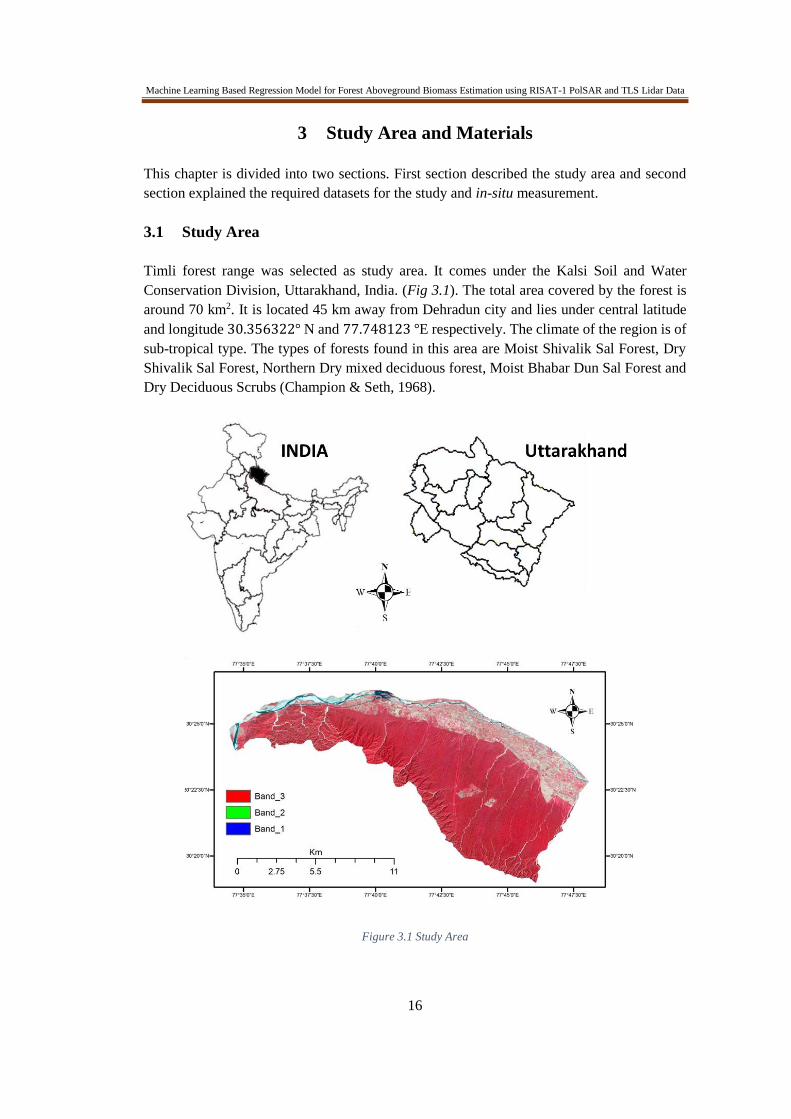
This chapter is divided into two sections. First section described the study area and second
section explained the required datasets for the study and in-situ measurement.
3.1 Study Area
Timli forest range was selected as study area. It comes under the Kalsi Soil and Water
Conservation Division, Uttarakhand, India. (Fig 3.1). The total area covered by the forest is
around 70 km2. It is located 45 km away from Dehradun city and lies under central latitude
and longitude 30.356322° N and 77.748123 °E respectively. The climate of the region is of
sub-tropical type. The types of forests found in this area are Moist Shivalik Sal Forest, Dry
Shivalik Sal Forest, Northern Dry mixed deciduous forest, Moist Bhabar Dun Sal Forest and
Dry Deciduous Scrubs (Champion & Seth, 1968).
Figure 3.1 Study Area

Machine Learning Based Regression Model for Forest Aboveground Biomass Estimation using RISAT-1 PolSAR and TLS Lidar Data
17
3.2 Materials
This section provides the details of various data used for the study. First section consists
satellite data and second section consists in-situ measurement using Terrestrial Lidar.
3.2.1 Satellite Data
RISAT-1 fully polarimetric data of 13th February 2014 was used for the study. The format of
data was in SLC (Single look complex). The complex data was stored in real and imaginary
aperture channel. It means data have amplitude as well as phase information. RISAT-1 is a
first Indian SAR satellite launched on 26th April, 2012. The satellite carries a multi-mode SAR
payload in C-band. It provides multi resolution, multi-swath and multi polarized data. The
specification of data is shown in Table 1.
Table 1 Specifications of RISAT-1 SAR Satellite (Anonymous, 2014)
Frequency (C-band) 5.35 GHz
Date of Acquisition 13-Feb-2014
Incidence angle 13.43275
Imaging Mode FRS-2
Swath 25 km
Polarization Quad
Slant Range Resolution 9mx4m
Central Latitude 30.447204
Central Longitude 77.777469
Orbit Direction Ascending
3.2.2 Terrestrial Laser Scanner
A ground based Laser instrument called Terrestrial Laser Scanner (TLS) (Fig 3.2) was used
for in-situ measurements of sample plots. This instrument is manufactured by Riegl Company
and VZ-400 model was for this study. The class 1 type laser was used and the wavelength lies
in near infrared region of electromagnetic spectrum. It has a beam divergence of 0.35 millirads
and an initial beam diameter of 0.007 m. The details of TLS specifications are shown in Table
2.
Table 2 Specification of Terrestrial Laser Scanner (Carr, 2013)
Range Up to 600m
Minimum Range 1.5 m
Measurement rate 122000 measurement per sec
Field of View 100x360
Accuracy 5 mm
Precision 3 mm

Machine Learning Based Regression Model for Forest Aboveground Biomass Estimation using RISAT-1 PolSAR and TLS Lidar Data
18
Laser Type Class 1
Laser Wavelength Near Infrared
Laser Beam Divergence 0.35 m rad
Weight Approx. 9.6kg
Figure 3.2 Riegl VZ-400 Instrument (Carr, 2013)
3.2.3 In-situ Measurement
The in-situ measurements and TLS data acquisition of sample plots were taken in the month
of March 2015. A total of 14 sample plots of 0.1 hectare size (31.62m x31.62m) were taken
and DBH of individual trees were measured using measuring tape. The random sampling
method was used for sampling. The location of sampled plots were shown in Fig 3.3.
The volume was calculated using species specific volumetric equations developed by Forest
Survey of India (FSI, 1996). The volumetric equation for sal tree is given as follows (3.1):
𝑉𝑜𝑙𝑢𝑚𝑒 = 0.03805 − 0.77794 ∗ 𝐷 + 8.42051 ∗ 𝐷2 + 5.91067 ∗ 𝐷3 (3.1)
The aboveground woody biomass was calculated as (3.2):
𝐴𝑏𝑜𝑣𝑒𝑔𝑟𝑜𝑢𝑛𝑑 𝑊𝑜𝑜𝑑𝑦 𝐵𝑖𝑜𝑚𝑎𝑠𝑠 = 𝑉𝑜𝑙𝑢𝑚𝑒 ∗ 𝑠𝑝𝑒𝑐𝑖𝑓𝑖𝑐 𝑔𝑟𝑎𝑣𝑖𝑡𝑦 (3.2)
The aboveground woody biomass was converted in to total AGB using the biomass expansion
factor (Haripriya, 2002).
𝐴𝐺𝐵 = 𝐴𝑏𝑜𝑣𝑒𝑔𝑟𝑜𝑢𝑛𝑑 𝑊𝑜𝑜𝑑𝑦 𝐵𝑖𝑜𝑚𝑎𝑠𝑠 ∗ 𝐵𝑖𝑜𝑚𝑎𝑠𝑠 𝑒𝑥𝑝𝑎𝑛𝑠𝑖𝑜𝑛 𝑓𝑎𝑐𝑡𝑜𝑟 (3.3)
For Sal trees, Specific gravity= 0.72 g/cc, Biomass expansion factor= 1.59. Using above
equations, field biomass was calculated and used as dependent variable for random forest
regression modelling.

Machine Learning Based Regression Model for Forest Aboveground Biomass Estimation using RISAT-1 PolSAR and TLS Lidar Data
19
Figure 3.3 Plot Sampling location in RISAT-1 Image

Machine Learning Based Regression Model for Forest Aboveground Biomass Estimation using RISAT-1 PolSAR and TLS Lidar Data
20
4 Methodology
To achieve the objectives of research work, methodology was divided into three parts (Fig
4.1). The first part includes radiometric calibration of RISAT-1 PolSAR data, covariance
matrix generation, various decomposition models to retrieve scattering variables (surface,
double bounce, volume, helix and wire scattering) and regression analysis between volume
scattering and field biomass. Second part consists basically processing of TLS Lidar data for
stem diameter and tree height estimation. In the end, multi-linear and random forest regression
algorithm is analyzed for predicting AGB. The above mentioned processes are explained in
later paragraphs.
Figure 4.1 Methodology

Machine Learning Based Regression Model for Forest Aboveground Biomass Estimation using RISAT-1 PolSAR and TLS Lidar Data
21
4.1 Radiometric Calibration
The receiving backscatter value is related to physical property of the targets (CSSTEAP
2011). The complex pixel value in the SAR image represent the digital number (DN) and it
does not associate with the ground target backscatter value. Radiometric calibration converts
the pixel values in the SAR image to quantitative representation of backscatter coefficient
(𝜎𝑜) (Anonymous, 2014; Kaasalainen et al., 2011). Backscatter coefficients are calculated by
normalizing the calculated backscatter by standard area and mathematically represents as
Radar cross section per unit area. If area is represented in slant range direction, it gives the
value of backscatter coefficient (𝛽𝑜), if in ground range, expressed as (𝜎𝑜) and if area in the
plane perpendicular to the slant range direction, then it estimates 𝛾𝑜 coefficient (Small &
Meier, 2013).
The equation (4.1) was used for calibration of RISAT-1 data as shown below. (Anonymous,
2014)
𝜎𝑜 =𝐷𝑁∗𝑆𝑖𝑛(𝑖𝑝)
𝑆𝑖𝑛(𝑖𝑐)∗𝑎𝑛𝑡𝑖𝑙𝑜𝑔10(𝑘
10) (4.1)
Where,
𝜎𝑜 = 𝑏𝑎𝑐𝑘𝑠𝑐𝑎𝑡𝑡𝑒𝑟 𝑣𝑎𝑙𝑢𝑒, 𝐷𝑁 = 𝑑𝑖𝑔𝑖𝑡𝑎𝑙 𝑣𝑎𝑙𝑢𝑒 𝑜𝑓 𝑝𝑖𝑥𝑒𝑙, 𝑖𝑐 = 𝑐𝑒𝑛𝑡𝑟𝑎𝑙 𝑖𝑛𝑐𝑖𝑑𝑒𝑛𝑐𝑒 𝑎𝑛𝑔𝑙𝑒
𝑖𝑝 = 𝑖𝑛𝑐𝑖𝑑𝑒𝑛𝑐𝑒 𝑎𝑛𝑔𝑙𝑒 𝑎𝑡 𝑝𝑖𝑥𝑒𝑙 𝑝, 𝑘 = 𝑐𝑎𝑙𝑖𝑏𝑟𝑎𝑡𝑖𝑜𝑛 𝑐𝑜𝑛𝑠𝑡𝑎𝑛𝑡 𝑖𝑛 𝑑𝐵
The above equation was applied on RISAT-1 data and Fig 4.2 shows the RISAT-1 HH
polarized image before and after radiometric calibration. The calibrated image gives the
backscattering coefficient value.
Figure 4.2 RISAT-1 HH image (i) before calibration (ii) after calibration

Machine Learning Based Regression Model for Forest Aboveground Biomass Estimation using RISAT-1 PolSAR and TLS Lidar Data
22
4.2 Multilooking
SAR sensor is side looking and data is captured in slant range direction. The resulting pixels
are rectangular in shape. To analyze the ground targets, ground range pixels are required.
Multilooking process converts the slant range pixels into ground range pixels. The pixels
shape is changed from rectangular to square. This process required no of looks that can be
determined by using the mathematical equation as shown below (4.2). (CSSTEAP, 2011)
𝑛𝑜 𝑜𝑓 𝑙𝑜𝑜𝑘𝑠 =𝑟𝑎𝑛𝑔𝑒 𝑟𝑒𝑠𝑜𝑙𝑢𝑡𝑖𝑜𝑛
𝑎𝑧𝑖𝑚𝑢𝑡ℎ 𝑟𝑒𝑠𝑜𝑙𝑢𝑡𝑖𝑜𝑛∗sin (α) (4.2)
Here α is the incidence angle of image
This formula was implemented on RISAT-1 data. Range resolution, azimuth resolution and
incidence angle information were given in metadata file.
Range resolution= 4.68 m, Azimuth resolution= 10 m, Incidence angle= 13.43275 degree.
From the above formula, no of looks = 2. Fig 4.3 shown the RISAT-1 image before and after
multilooking.
Figure 4.3 Shown the image before and after Multilooking

Machine Learning Based Regression Model for Forest Aboveground Biomass Estimation using RISAT-1 PolSAR and TLS Lidar Data
23
4.3 Polarimetric Decomposition Modelling
The SLC (single look complex) data was stored in scattering matrix format. The covariance
matrix was used for the extracting the information from natural targets (refer to 2.2). The
decomposition models decomposed the covariance matrix into various scattering mechanism
that can be physically interpreted.
This study used the 3-component model by Vanzyl (Lee & Pottier, 2009), 4-component model
by Yamaguchi (Yamaguchi et al., 2005) and 5-component model by Zhang (Zhang et al.,
2008). The purpose of using all three models will to check the feasibility of the model on
RISAT-1 for biomass modelling.
4.3.1 Types of Decomposition Models
4.3.1.1 Van-zyl Decomposition
The van-Zyl based decomposition is a type of 3-component decomposition modelling
approach based on Eigen values and Eigen vectors. It uses the 3x3 covariance [𝐶] matrix for
azimuthally symmetrical terrain. The model assumes that the correlation between the cross
polarization and co-polarized power is zero and holds the condition of reflection symmetry.
i.e. < 𝑆𝐻𝐻𝑆𝐻𝑉∗ >≈< 𝑆𝑉𝑉𝑆𝐻𝑉
∗ >≈ 0. It means the effect of 𝐶12, 𝐶21, 𝐶23 and 𝐶32 components
can be ignored. This model is suitable to describe the polarimetric backscatter from natural
targets. It follows the corresponding averaged covariance matrix given by (Lee & Pottier,
2009). The 3x3 covariance matrix can be expressed as shown in equation (4.3)
[𝐶] = 𝑓𝑠𝐶𝑠𝑢𝑟𝑓𝑎𝑐𝑒 + 𝑓𝑑𝐶𝑑𝑜𝑢𝑏𝑙𝑒 𝑏𝑜𝑢𝑛𝑐𝑒 + 𝑓𝑣𝐶𝑣𝑜𝑙𝑢𝑚𝑒 (4.3)
The detailed mathematical expression was explained in appendix 2. The Vanzyl decomposed
results of RISAT-1 data was shown in Fig 4.4.
Figure 4.4 Vanzyl decomposed results. Left side image is surface scattering, middle image is double bounce scattering and last image is volume scattering

Machine Learning Based Regression Model for Forest Aboveground Biomass Estimation using RISAT-1 PolSAR and TLS Lidar Data
24
4.3.1.2 Yamaguchi decomposition
Van Zyl’s 3-component decomposition technique is reliable for planar surface and the
correlation between the cross-pol and co-pol power is very less which can be ignored. But for
rough terrain surfaces, this correlation cannot be ignored. Yamaguchi proposed a model
without assumption of reflection symmetry condition and considered the effects of
< 𝑆𝐻𝐻 𝑆𝐻𝑉∗ ≠ 0 > and < 𝑆𝑉𝑉 𝑆𝐻𝑉
∗ ≠ 0 > components taken into account. It is the extension
of 3-component modelling approach. In addition, a 4th component was introduced called Helix
scattering which occurs due to complex structures of targets. The decomposition is expressed
in equation shown below (4.4). (Han & shao, 2010; Yamaguchi et al., 2005)
[𝐶] = 𝑓𝑠𝐶𝑠𝑢𝑟𝑓𝑎𝑐𝑒 + 𝑓𝑑𝐶𝑑𝑜𝑢𝑏𝑙𝑒 𝑏𝑜𝑢𝑛𝑐𝑒 + 𝑓𝑣𝐶𝑣𝑜𝑙𝑢𝑚𝑒 + 𝑓𝑐𝐶ℎ𝑒𝑙𝑖𝑥 (4.4)
𝑓𝑠, 𝑓𝑑, 𝑓𝑣 and 𝑓𝑐 are the expansion coefficients.
This fourth component corresponds mostly in complex settlement areas like stadium structure
and complicated tree structures. The Yamaguchi decomposition results on RISAT-1 data was
shown in Fig 4.5 below.
Figure 4.5 Yamaguchi decomposition results. Starts from left image surface scattering, double bounce
scattering, volume scattering and helix scattering
4.3.1.3 Multi-component Decomposition
Zhang et al. (2008) proposed multi-component decomposition modelling approach consisting
five components including wire scattering. Wire scattering is a specific scattering component
which is linked with the cross-polarized powers. The decomposition is expressed in equation
(4.5).
[𝐶] = 𝑓𝑠𝐶𝑠𝑢𝑟𝑓𝑎𝑐𝑒 + 𝑓𝑑𝐶𝑑𝑜𝑢𝑏𝑙𝑒 𝑏𝑜𝑢𝑛𝑐𝑒 + 𝑓𝑣𝐶𝑣𝑜𝑙𝑢𝑚𝑒 + 𝑓ℎ𝐶ℎ𝑒𝑙𝑖𝑥 + 𝑓𝑤𝐶𝑤𝑖𝑟𝑒 (4.5)

Machine Learning Based Regression Model for Forest Aboveground Biomass Estimation using RISAT-1 PolSAR and TLS Lidar Data
25
= 𝑓𝑠 [|𝛽|2 0 𝛽0 0 0𝛽∗ 0 1
] + 𝑓𝑑 [|𝛼|2 0 𝛼0 0 0
𝛼∗ 0 1
] +𝑓𝑣15
[8 0 2 0 4 02 0 3
] +𝑓𝑐4
[
1 ±𝑗√2 −1
∓𝑗√2 4 ±𝑗√2
−1 ∓𝑗√2 1
]
+ 𝑓𝑤 [
|𝛾|2 √2𝛾𝜌∗ 𝛾
√2𝛾∗𝜌 2|𝜌|2 √2𝜌
𝛾∗ √2𝜌∗ 1
]
Where𝑓𝑠, 𝑓𝑑, 𝑓𝑣, 𝑓ℎ, 𝑓𝑤 are the coefficients.
By comparing the covariance elements, the coefficients can be expressed as:
< |𝑆𝐻𝐻|2 > = 𝑓𝑠|𝛽|2 + 𝑓𝑑|𝛼|2 + 𝑓𝑣 +1
4𝑓ℎ + 𝑓𝑤|𝛾|2), (4.6)
< 𝑆𝑉𝑉|2 >= 𝑓𝑠 + 𝑓𝑑 + 𝑓𝑣 +1
4𝑓ℎ + 𝑓𝑤 (4.7)
< 𝑆𝐻𝐻𝑆𝑉𝑉∗ >= 𝑓𝑠𝛽 + 𝑓𝑑𝛼 +
1
3𝑓𝑣 −
1
4𝑓ℎ + 𝑓𝑤𝛾, (4.8)
< |𝑆𝐻𝑉|2 >=1
3𝑓𝑣 +
1
4𝑓ℎ + 𝑓𝑤|𝜌|2 (4.9)
< 𝑆𝐻𝐻𝑆𝐻𝑉∗ >= ±𝑗
1
4𝑓ℎ + 𝑓𝑤𝛾𝜌∗ , (4.10)
< 𝑆𝐻𝑉𝑆𝑉𝑉∗ >= ±𝑗
1
4𝑓ℎ + 𝑓𝑤𝜌 (4.11)
Helix scattering coefficient 𝑓ℎ and wire scattering coefficient 𝑓𝑤 can be calculated using the
equation (4.10) and (4.11) as shown below. (Zhang et al., 2008)
𝑓𝑤 =<𝑆𝐻𝐻𝑆𝐻𝑉
∗ >−<𝑆𝐻𝑉𝑆𝑉𝑉∗ >
𝛾𝜌∗−𝜌 (4.12)
𝑓ℎ = 2𝐼𝑚{< 𝑆𝐻𝐻𝑆𝐻𝑉∗ > +< 𝑆𝐻𝑉𝑆𝑉𝑉
∗ > −𝑓𝑤(𝛾𝜌∗ + 𝜌)}
The remaining coefficient can be calculated in the same manner using above mentioned
equations (4.7, 4.8 and 4.9). The scattering powers for double bounce, volume, odd bounce,
wire and helix scattering are shown below and the equation (4.13) shows the total power.
𝑃𝑠 = 𝑓𝑠(1 + |𝛽|2), 𝑃𝑑 = 𝑓𝑑(1 + |𝛼|2), 𝑃𝑣 = 8𝑓𝑣/3, 𝑃ℎ = 𝑓ℎ,
𝑃𝑤 = 𝑓𝑤(1 + |𝛾|2 + 2|𝜌|2),
𝑃 = 𝑃𝑠 + 𝑃𝑑 + 𝑃𝑣 + 𝑃ℎ + 𝑃𝑤 (4.13)

Machine Learning Based Regression Model for Forest Aboveground Biomass Estimation using RISAT-1 PolSAR and TLS Lidar Data
26
The multi-component decomposition equations shows the correlation behaviour between the
co-polarised powers and cross-polarised powers which is not observed in 3-component
decomposition modelling. The results of multi-component decomposition results on RISAT-
1 data is shown below Fig 4.6.
Figure 4.6 MCMS decomposition results. Start from the left image, surface scattering, double bounce scattering, volume scattering, helix scattering and wire scattering
4.4 Feasibility Analysis of Polarimetric Decomposition Models
This section will check the suitability of polarimetric decomposition models for biomass
modelling approach. From the semi-empirical modelling approach (Jochem et al., 2011;
Poolla, 2013) the volume scattering is more contributing for biomass modelling and it was
found directly proportional to Biomass. A regression analysis will be conducted between field
collected Biomass and volume scattering computed from above decomposition models. The
result of this output decides which decomposition model parameters will be used for biomass
modelling.
4.5 TLS Lidar data Processing
Terrestrial Lidar data processing were done in three phases. First phase involves the data
acquisition. Second phase included the registration of individual scan and merging of point
cloud data and third phase estimated the stem diameter and tree height of an individual tree.
4.5.1 TLS Data Acquisition
TLS data acquisition of 14 sample plots were taken in the month of March 2015. The
geometry of each plot was square (31.6 m x 31.6 m) and area was 0.1 hectare (Fig 4.7). The
random sampling method was used for sampling. The workflow of data acquisition was
shown in Fig 4.8. After making the boundary of sample plot, the first step is to place the retro-
reflector targets within the plot. Then, TLS position was examined within or outside the plots
so that maximum coverage of the target is captured with minimum occlusion effect. The
positions were shown in geometry plot. In this study three scans were taken in such a way

Machine Learning Based Regression Model for Forest Aboveground Biomass Estimation using RISAT-1 PolSAR and TLS Lidar Data
27
that at least 3 reflectors were seen from each position. The scanner was then started with a
panorama scan (360 horizontal) of the target along with digital photographs. The angular
resolution was selected as 0.03 degree in both horizontal and vertical direction. Around
40011334 points were returned from the target within 15 min 48 second time (refer to
appendix 1). These three scans were named as central scan, scan 1 and scan 2 as shown in Fig
15. The reflectors were act as control tie points. The next step was to do fine scan of control
tie points. It will scan only the reflectors with high dense cloud. This step is necessary for
registration of point cloud. After each scan, TLS was moved to next position and reflector
position remain same. The reflectance of the scanned material, visibility limitations due to
dust and topographic relief can affect the quality of the returned data. The quality of data was
accessed during registration.
The laser scanner was operated by RISCAN Pro software which comes along with the
instrument. In Riegl VZ-400 instrument, it has scanning range of 360 degree horizontal and
100 degree in vertical direction. The density of data was dependent on project requirement
and scan parameters (refer to appendix 1). The high resolution camera is mounted on top of
instrument captured intensity value of the target. The color intensity value was merged to the
reflectance image of the cloud. Fig 4.9 shows the reflectance image and same after merging
color intensity value to the cloud. Initially point cloud was assigned to the SOCS (Scanner
own coordinate system). The position and orientation of the scanner can be described by the
4x4 MSOP matrix (SOP means sensor’s orientation and position) in equation (4.14). The
matrix contains nine rotational parameters (r11 to r33) and three translation parameters (t1 to
t3).
𝑀𝑆𝑂𝑃 = [
𝑟11 𝑟12 𝑟13 𝑡1𝑟21 𝑟22 𝑟23 𝑡2𝑟31 𝑟32 𝑟33 𝑡30 0 0 1
] (4.14)
Figure 4.7 Geometry of sample plots

Machine Learning Based Regression Model for Forest Aboveground Biomass Estimation using RISAT-1 PolSAR and TLS Lidar Data
28
Figure 4.8 Workflow of TLS Data Acquisition in multiple scanning
Figure 4.9 left side image shown the reflectance image of a sampled plot and right side image display the point cloud after assigning the color intensity
4.5.2 Point Cloud Registration
Initially the point cloud scans were unregistered. Multiple scans were registered on the basis
of common tie points. One scan position was selected as reference scan. Here, central scan
(Fig 4.10) was called as reference scan. With respect to central scan, scan 1 and scan 2 were
registered. Each scan has at least 4 to 5 common tie-points. The automatic registration process
was performed between two scans. This technique finds the common tie points between two
scans and data points are multiplied with the SOP matrix (𝑀𝑆𝑂𝑃) of the scan position. Then,
after registration process, the coordinated system has transferred from SOCS to PRCS (Project
Coordinate System) (for more details refer to appendix 1). Another technique named as
manual registration in which common tie-points have to be found manually. This process is
time consuming and not feasible for this study. In RISCAN PRO, this process was operated
in minimized error mode with 0.1 tolerance and minimum 6 common tie point (see results in
appendix 1). After the process was over, standard deviation of 0.0196 was achieved which
was less than 0.1 and acceptable. The registered scans were merged to each other and 3D
model (Fig 4.11) was generated.

Machine Learning Based Regression Model for Forest Aboveground Biomass Estimation using RISAT-1 PolSAR and TLS Lidar Data
29
Figure 4.10 sampled plot scans captured from the different scan position and shadow was appeared behind the trees due to occlusion effect
Figure 4.11 3D tree model generated after merged all scans. The disappear of shadow was indicated that occlusion effect was removed

Machine Learning Based Regression Model for Forest Aboveground Biomass Estimation using RISAT-1 PolSAR and TLS Lidar Data
30
4.5.3 Individual Tree extraction
The merged cloud of the plot consists large number of trees. Due to high dense cloud, the size
of data was very large and it was not easy to handle it. Processing of large amount of data
required high computation device and the time of processing was also very high. This study
extracted individual tree samples and processed separately. The format of data was a text file
with x, y, z coordinates. The 3D point cloud of an individual tree stem was in cylindrical
shape but not perfectly as shown in Fig 4.12. This irregular shape of cylinder does not provide
the accurate measurement of diameter. So, this cylindrical structure was cross-sectioned by a
section of plane at z=1 (Fig 4.12). The circle structure was cut and examined separately. It
consisted the set of x, y points and a circle was fit using least square method that was explained
in next section.
Figure 4.12 (i) irregular tree structure (ii) Cylinder cross-section at z=1 plane
4.6 Stem diameter Estimation using Least Square Circle Fit
The least square algorithm is based on minimize the sum of squared distances from the data
points to the fitting circle. For each point, there are two variables i.e. (x, y) coordinates of
point’s position. If the centre of the circle is at (a, b) and the position of a point is (x, y), then
from the Pythagoras theorem, the distance from the centre to the point is described in equation
(4.15) (Bullock, 2006):
√(𝑥 − 𝑎)2 + (𝑦 − 𝑏)2 (4.15)
But the aim of this algorithm is to find the distance from the fitted circle to the point. Since
the radius of circle is R, the distance from the perimeter to the point (along a straight line from
the centre to the point) is shown in equation (4.16). That is, the distance from the fitting circle
to the point is equal to the distance from the centre to the point minus the radius.

Machine Learning Based Regression Model for Forest Aboveground Biomass Estimation using RISAT-1 PolSAR and TLS Lidar Data
31
√(𝑥 − 𝑎)2 + (𝑦 − 𝑏)2 − 𝑅 (4.16)
The distance will be positive or negative depending on whether the point is outside or inside
the circle, but this does not matter since the value is squared as part of the minimization
process. Hence, the minimization function is shown in equation (4.17). In this problem, the
two parameters i.e. centre (a, b) and Radius (R) has to be determined (Chernov & Lesort,
2005).
𝐹1(𝑎, 𝑏, 𝑅) = ∑ [(𝑥 − 𝑎)2 + (𝑦 − 𝑏)2 − 𝑅2]2𝑛𝑖=1 = ∑ [𝑃(𝑥, 𝑦)2]𝑛
𝑖=1
= [𝑥𝑖2 + 𝑦𝑖
2 + 𝑎2 + 𝑏2 − 2 ∗ 𝑥𝑖 ∗ 𝑎 − 2 ∗ 𝑦𝑖 ∗ 𝑏 − 𝑅2]
= [𝑧𝑖 + 𝐵𝑥𝑖 + 𝐶𝑦𝑖 + 𝐷] (4.17)
Where 𝑧𝑖 = 𝑥𝑖2 + 𝑦𝑖
2, 𝐵 = −2𝑎, 𝐶 = −2𝑏, 𝐷 = 𝑎2 + 𝑏2 − 𝑅2
The above described objective function is based on simple algebraic fit and fitting curve is
described by an implicit polynomial function 𝑃(𝑥, 𝑦) = 0 (equation 4.18) and the coefficients
of polynomial function gives the parameters of curve.
Another method called gradient weighted algebraic fit (GRAF), which is based on minimizing
objective function 𝐹 as shown in equation 5.
𝐹 = ∑[𝑃(𝑥𝑖,𝑦𝑖)]
2
‖∇𝑃(𝑥𝑖,𝑦𝑖)‖2
𝑛𝑖=1 (4.18)
Here ∇𝑃(𝑥, 𝑦) is the gradient olf the function 𝑃(𝑥, 𝑦). In this method, the equation 4 is
modified, by multiplying a factor A as shown below in equation 4.24:
𝑃(𝑥, 𝑦) = [𝐴(𝑥2 + 𝑦2) + 𝐵𝑥 + 𝐶𝑦 + 𝐷] (4.19)
It can be said that, the equation 6 can hold for simple algebraic fit under the constraint A=1.
Now, equation (4.19) is partially differentiating w.r.t 𝑥 and 𝑦 and the solution is shown in
equation (4.20). ∇𝑃(𝑥, 𝑦) = (2𝐴𝑥 + 𝐵, 2𝐴𝑦 + 𝐶)
‖∇𝑃(𝑥, 𝑦)‖2 = 4𝐴𝑧2 + 4𝐴𝐵𝑥 + 4𝐴𝐶𝑦 + 𝐵2 + 𝐶2
= 4𝐴(𝐴𝑧 + 𝐵𝑥 + 𝐶𝑦 + 𝐷) + 𝐵2 + 𝐶2 − 4𝐴𝐷 (4.20)
Now, the objection function of GRAF reduced to the minimization:
𝐹 = ∑[(𝐴𝑧𝑖+𝐵𝑥𝑖+𝐶𝑦𝑖+𝐷)]2
4𝐴(𝐴𝑧𝑖+𝐵𝑥𝑖+𝐶𝑦𝑖+𝐷)+𝐵2+𝐶2−4𝐴𝐷𝑛𝑖=1 (4.21)

Machine Learning Based Regression Model for Forest Aboveground Biomass Estimation using RISAT-1 PolSAR and TLS Lidar Data
32
4.6.1 Pratt’s Method for minimization
Pratt’s assumes that, if data points lie close to the circle, then 𝐴𝑧𝑖 + 𝐵𝑥𝑖 + 𝐶𝑦𝑖 + 𝐷 ≈ 0 and
proposed a new objective function (equation 4.22) who clearly describe its advantages over
the simple algebraic fit. (Pratt, 1987)
𝐹𝑝𝑟𝑎𝑡𝑡 = ∑[(𝐴𝑧𝑖+𝐵𝑥𝑖+𝐶𝑦𝑖+𝐷)]2
𝐵2+𝐶2−4𝐴𝐷𝑛𝑖=1 (4.22)
Pratt minimizes the 𝐹𝑝𝑟𝑎𝑡𝑡 by using matrix method. The minimization is equivalent to
minimization of simpler function (equation 4) subject to the constraint such that 𝐵2 + 𝐶2 −
4𝐴𝐷 = 1.
The numerator term of 𝐹𝑝𝑟𝑎𝑡𝑡 is written in matrix form as, 𝐹𝑛𝑢𝑚 = 𝑨𝑻𝑴𝑨, where
𝑨 = (𝐴, 𝐵, 𝐶, 𝐷)𝑇 is the vector of parameters and 𝑴 is the matrix of moments as shown below
(equation 4.23).
𝑴 =
[ 𝑀𝑧𝑧 𝑀𝑥𝑧
𝑀𝑥𝑧 𝑀𝑥𝑥
𝑀𝑦𝑧 𝑀𝑧
𝑀𝑥𝑦 𝑀𝑥
𝑀𝑦𝑧 𝑀𝑥𝑦
𝑀𝑧 𝑀𝑥
𝑀𝑦𝑦 𝑀𝑦
𝑀𝑦 𝑛 ]
(4.23)
Where,𝑀𝑥𝑥 = ∑𝑥2, 𝑀𝑦𝑦 = ∑𝑦2, 𝑀𝑥𝑦 = ∑𝑥𝑖𝑦𝑖 etc.
An important point is to be noted that, 𝑴 is symmetric and positive semi-definite. The
constraint 𝐵2 + 𝐶2 − 4𝐴𝐷 − 1 = 0 can be written as 𝑨𝑻𝑩𝑨 − 𝟏 = 𝟎 and B matrix is
explained in equation (4.24).
Where
𝑩 = [
0 00 1
0 −20 0
0 0−2 1
1 00 0
] (4.24)
Now introduce Lagrange method for minimizing, 𝐹𝑛𝑢𝑚,
𝐹(𝐴, 𝜂) = 𝑨𝑻𝑴𝑨 − 𝜂(𝑨𝑻𝑩𝑨 − 𝟏) (4.25)
Differentiating equation (4.25) with respect to A gives,= 𝜂𝑩𝑨 , 𝜂 is the generalized eigen
value for the matrix pair (𝑴,𝑩) and A is corresponding generalized eigenvector. The matrix
B is symmetric and has four Eigen values (1, 1, 2,-2). If M is positive definite, by Sylvester’s
law of inertia the generalized eigenvalue of matrix pair (𝑴,𝑩) are all real and exactly three
of them are positive and one is negative. Now the function 𝐹𝑝𝑟𝑎𝑡𝑡 becomes, (equation 4.26)
𝐹𝑝𝑟𝑎𝑡𝑡 = 𝑨𝑻𝑴𝑨 = 𝜂𝑨𝑻𝑩𝑨 = 𝜂 (4.26)

Machine Learning Based Regression Model for Forest Aboveground Biomass Estimation using RISAT-1 PolSAR and TLS Lidar Data
33
Hence the minimum of 𝐹𝑝𝑟𝑎𝑡𝑡 corresponds to smallest non-negative generalized eigenvalue.
Generalized Eigen pairs (𝜂, 𝑨) can be found by standard matrix methods. The computation
time of this method is quite high. An alternate solution to this problem is polynomial equation
(4.27) solved by newton’s method starting at 𝜂 = 0.
𝑄4(𝜂) = det(𝑀 − 𝜂𝐵) = 0 (4.27)
Newton’s iteration are useful to converge to the smallest non-negative root, because
polynomial function 𝑄4(𝜂) is decreasing and concave up between 0 and 𝜂∗
𝜂∗ = min {𝜂 ≥ 0: 𝑄4(𝜂) = 0 }
This mathematical function was implemented in MATLAB. Due to variation of CBH with
height, this study measure the stem diameter at z=1 height from the ground. The set of (x, y)
points at z=1 was taken from TLS individual tree data.
4.7 Modelling Approach for AGB Estimation
This section explained the two models for AGB estimation. The first one is Multi-Linear
Regression Modelling approach and another is Random Forest Modelling approach. The input
parameters for the models was selected on the basis of results of feasibility analysis of
polarimetric decomposition models.
Here, Multi-linear regression modelling approach was developed only for SAR parameters to
study the potential of RISAT-1 data and another was machine learning based Random forest
regression model which used the integration of SAR and TLS Lidar estimated biophysical
parameters. The accuracy of both models were compared.
4.8 Multiple Linear Regression Modelling approach
Regression is the process in which variation of one variable is explained by the variation of
more number of variables. It is the statistical process used to establish the relationship among
variables. Variables can be categorized as independent and dependent variables. (Stein et al.,
2002). Equation (4.28) shows the generalized regression expression.
𝑌 = 𝑎𝑋1 + 𝑏𝑋2 + 𝑐𝑋3 + 𝑑𝑋4 + ⋯+ 𝑛𝑋𝑛 (4.28)
𝑋1, 𝑋2, 𝑋3, 𝑋4, …𝑋𝑛 are the independent variables and Y is the dependent variable.
In this study, biomass was the dependent variable and SAR variables i.e. double bounce,
Volume, Surface and helix scattering were the independent variables. From the given
observations, two models were generated and the hypothesis tests was used for validating the
significance of coefficients.

Machine Learning Based Regression Model for Forest Aboveground Biomass Estimation using RISAT-1 PolSAR and TLS Lidar Data
34
4.8.1 Regression model
4.8.1.1 Scatter Plot
Before developing the regression model, there was need to investigate how SAR variables
were related to each another. The scatter plot will represent the correlation. Fig 4.13 explained
the scatterplot of each variable.
Figure 4.13 show the correlation of each variable
4.8.1.2 Multi-Collinearity test between independent variables
Then multi-collinearity test will check how two independent variables are correlated with
each other. The correlation between each SAR variables viz. Double bounce, Volume, Surface
and Helix were checked and their statistical value were shown in Table 3.
Table 3 Describe the Correlation of each independent variable with respect to each other
Variable 1 Variable 2 Correlation
Double Bounce Volume -0.099
Double bounce Surface 0.2732
Double Bounce Helix -0.0664
Volume Surface 0.6227
Volume Helix -0.2886
Surface Helix 0.0597
4.8.1.3 Hypothesis Test
This test check the significance of whole regression model. The statement of Hypothesis are:

Machine Learning Based Regression Model for Forest Aboveground Biomass Estimation using RISAT-1 PolSAR and TLS Lidar Data
35
𝐻𝑜 = 𝛽1 = 𝛽2 = 𝛽3 = ⋯ = 𝛽𝑛 = 0 , 𝐻1 = 𝛽1, 𝛽2, 𝛽3, 𝛽𝑛 ≠ 0
Here, 𝛽𝑘 are the coefficients of regression model. (Chatterjee & Hadi, 2006)
Test to find the significance of regression coefficients
F-test: this test checks the significance of regression coefficients. This test is not significant
if model has more than one variable.
T-test: this test encounters the significance of individual regression coefficients. (Dixon &
Massey, 1969)
F-Test
Step 1: Calculate the critical f-value.
It can be calculated by F-distribution or cumulative distribution function (CDF) as shown by
equation (4.29).
𝐹(𝛼, 𝑑1, 𝑑2) = 𝐼 𝑑1𝑥
𝑑1𝑥+𝑑2
(𝑑1/2, 𝑑2/2) (4.29)
Where I is the regularized lower incomplete beta function. 𝑑1 𝑎𝑛𝑑 𝑑2 are the degrees of
freedom and 𝛼 is the significance level. The formula is shown in equation (4.30).
𝐼𝑥(𝑎, 𝑏) =𝐵(𝑥,𝑎,𝑏)
𝐵(𝑎,𝑏) (4.30)
Where the numerator is the lower incomplete beta function, and the denominator is the beta
function explained in equation (4.31) and (4.32).
𝐵(𝑥, 𝑎, 𝑏) = ∫ 𝑡𝑎−1𝑥
0(1 − 𝑡)𝑏−1𝑑𝑡 (4.31)
𝐵(𝑥, 𝑦) = ∫ 𝑡𝑥−11
0(1 − 𝑡)𝑦−1𝑑𝑡 (4.32)
T-test
T-distribution cumulative distribution function
This formula in equation (4.33) is used for the calculation of critical t-values.
∫ 𝑓(𝑢) 𝑡
−∞𝑑𝑢 = 𝐼 (
𝑡+√𝑡2+𝑣
2√𝑡2+𝑣|
𝑣
2,𝑣
2) (4.33)
Where, v is the degrees of freedom, t is the upper limit of integration, and I is the regularized
lower incomplete beta function.

Machine Learning Based Regression Model for Forest Aboveground Biomass Estimation using RISAT-1 PolSAR and TLS Lidar Data
36
The t-values can be calculated as: 𝑡𝛽^ =𝛽^
𝑠𝑡𝑑 𝑒𝑟𝑟𝑜𝑟(𝛽^) (4.34)
4.8.1.4 Variance Inflation Factor (VIF)
It was the measure of how much the variance of an estimated regression coefficient increases
if the coefficients are correlated. It was used an indicator of multi-collinearity (O’brien, 2007).
4.9 Random Forest Regression modelling approach for AGB Estimation
4.9.1 Random Forest Approach
In decision tree, only a single tree was constructed. If there is any small change in data, it can
adversely affect the structure of tree. To improve the performance of the tree, ensemble
methods like Random Forest where many trees were fit and predictions were aggregated
across the trees. This study has used the Random Forest approach.
Fig 4.14 explained the flow diagram of random forest algorithm. A total number of 14 samples
as original dataset were used in this study. Around 8 random samples (2/3rd data) were used
as training data to train the model and 6 samples (1/3rd data) were used as test data. From the
training data, 8 bootstrap samples were drawn. The bootstrap sample means sample with
replacement. From the bootstrap samples, large number of decision trees (ntree) i.e. 500,
1000, 1500, 2000 etc. were grown using CART algorithm. During the growing decision tree,
it took the random subset (𝑚𝑡𝑟𝑦 =7
3~2) of predictors i.e. surface, double bounce, volume,
wire, helix, stem diameter, tree height for the splitting the each node. The splitting of node
was based on Gini index criteria. The two variables (mtry and ntree) need to be optimized for
accurate prediction. The same process (growing decision tree) is repeat again and again. The
optimization of variables was based on the minimization of out of bag error (RMSE)
calculated using the test data. The final output (biomass) was the average of output from each
tree.

Machine Learning Based Regression Model for Forest Aboveground Biomass Estimation using RISAT-1 PolSAR and TLS Lidar Data
37
Figure 4.14 Random Forest Approach
4.10 Validation (Accuracy Assessment) and sensitivity analysis
The stem diameter estimated from TLS data was validated with the ground measurements.
The predicted biomass from the model was regression analyzed with the field biomass and
coefficient of determination and root mean square error was calculated for validating the
output of model. The sensitivity of variables was decided on the basis of ranking of variables.
The priority decides the order of sensitivity.

Machine Learning Based Regression Model for Forest Aboveground Biomass Estimation using RISAT-1 PolSAR and TLS Lidar Data
38
5 Result and Discussion
The methodology was applied on RISAT-1 PolSAR data and TLS Lidar data. Their results
and analysis were described in this chapter.
5.1 Radiometric Calibration of RISAT-1 data
RISAT-1 FRS-2 data was radiometrically calibrated using mathematical equation as
described in equation 3.1. The effects due to atmospheric disturbances, bias due to antenna
aperture were removed. The statistical parameters were described in the frequency
distribution histogram plot (Fig 5.1). The {min, max} value before calibration is {-32766,
32767} represents the digital number of 16-bit radiometric data and after calibration is {-
17.634, 43.492} represented the normalized backscatter coefficient of the target. The scale of
data value was between 0 and 1. The purpose of radiometric calibration was to compare the
results of RISAT-1 with different sensors (Kaasalainen et al., 2011). This study does not
calculate calibration constant using field instruments. On the basis of given calibration
constant in RISAT-1 user guide, (Anonymous, 2014) RISAT-1 data is calibrated. The quality
of data assessment is not in the part of study. The calibrated image is required to generate the
PolSAR scattering matrix.
Figure 5.1 Histogram plot with statistical parameters (i) before calibration (ii) after calibration

Machine Learning Based Regression Model for Forest Aboveground Biomass Estimation using RISAT-1 PolSAR and TLS Lidar Data
39
5.2 Scattering Parameters retrieval using Polarimetric Decomposition Model
In a single SAR resolution cell, different scattering mechanism like surface scattering (𝑃𝑆),
double bounce scattering (𝑃𝑑), volume scattering (𝑃𝑣), helix scattering (𝑃ℎ) and wire scattering
(𝑃𝑤) was retrieved using polarimetric decomposition models. This study has tested Vanzyl
decomposition model (𝑉𝑚𝑜𝑑𝑒𝑙), Yamaguchi decomposition model (𝑌𝑚𝑜𝑑𝑒𝑙), and Multi-
component decomposition model (𝑀𝑚𝑜𝑑𝑒𝑙). Their results and analysis were described in next
paragraph.
𝑉𝑚𝑜𝑑𝑒𝑙 was applied on RISAT-1 PolSAR data and three scattering parameters viz. 𝑃𝑆, 𝑃𝑑 and
𝑃𝑣 were retrieved. Fig 5.2 visualize these parameters in RGB color combination, where R
represent the 𝑃𝑑, G represent the 𝑃𝑣 and B represent the 𝑃𝑆. The features like water bridge,
mountains, riverbed, forest patch and human settlement were found in the image. The green
color in lower part of image representing volume scattering from the forested area. Violet
color portion in middle of image shows the river bed where surface and double bounce
scattering was predominant. The mountains and water bridge was clearly visible in Fig 5.3
and compared it with the google earth image. Black region indicates no scattering value
retrieved due to specular reflection from the water bridge. The high backscattering value in
upper portion of mountain regions was due to foreshortening effects and dark tone next to it
due to shadow regions of mountains slope where no scattering occurs.
𝑌𝑚𝑜𝑑𝑒𝑙 has successfully retrieved 𝑃ℎ (Yamaguchi et al., 2005) while 𝑀𝑚𝑜𝑑𝑒𝑙 (Zhang et al.,
2008) has retrieved 𝑃ℎ and 𝑃𝑤 in addition to above three parameters. Fig 5.4 analyzed the
helix and wire scattering from the forest patch of Timli region. The intermediate brightness
pixels in the images indicate the presence of helix and wire scattering from the tree.
Theoretically, helix scattering comes from the circular shape of the target (Yamaguchi et al.,
2005) and sharpness of target can cause wire scattering like window frames (Zhang et al.,
2008). It is found that the circular shape of tree stem can be the cause of helix scattering. The
sharpness of tree leaves in canopy layer can cause wire scattering. The RGB view of
decomposition results of 𝑌𝑚𝑜𝑑𝑒𝑙 and 𝑀𝑚𝑜𝑑𝑒𝑙 was shown in Fig 5.5.

Machine Learning Based Regression Model for Forest Aboveground Biomass Estimation using RISAT-1 PolSAR and TLS Lidar Data
40
Figure 5.2 Vanzyl decomposed RGB image consisting surface, double bounce and volume scattering. The
features are identified as mountains, water bridge and river bed. The black box indicate the two subset which were shown in Fig 22.
Figure 5.3 The subset of the mountain and water bridge was compared with the google earth image.

Machine Learning Based Regression Model for Forest Aboveground Biomass Estimation using RISAT-1 PolSAR and TLS Lidar Data
41
Figure 5.4 compared the helix scattering and wire scattering in forest patch..The bright pixels in the image shows the presence of helix and
Figure 5.5 The RGB image of Yamaguchi and Multi-component Decomposition
5.3 Feasibility Analysis of Decomposition Models
This section will check the suitability of decomposition models for biomass modelling
approach.

Machine Learning Based Regression Model for Forest Aboveground Biomass Estimation using RISAT-1 PolSAR and TLS Lidar Data
42
5.3.1 Comparative study of volume scattering retrieved from decomposition models
The volume scattering retrieved in Timli region by 𝑉𝑚𝑜𝑑𝑒𝑙 , 𝑌𝑚𝑜𝑑𝑒𝑙 and 𝑀𝑚𝑜𝑑𝑒𝑙 (shown in
Fig 5.6) was compared in this section. The pixels brightness was high in 𝑌𝑚𝑜𝑑𝑒𝑙 and 𝑀𝑚𝑜𝑑𝑒𝑙
as compared to 𝑉𝑚𝑜𝑑𝑒𝑙. It shows that the backscattering coefficient of volume scattering was
low in 𝑉𝑚𝑜𝑑𝑒𝑙. The regression analysis was performed between field biomass and volume
scattering retrieved from above decomposition models. Fig 5.7 shows the trend of regression
line. The volume scattering was in linear relationship with field biomass. The high correlation
from 𝑀𝑚𝑜𝑑𝑒𝑙 i.e. R2= 0.17 and low correlation from 𝑉𝑚𝑜𝑑𝑒𝑙 i.e. R2= 0.06 was obtained. The
results was dependent on the volume scattering value and volume equation used by
decomposition model. The volume scattering from 𝑉𝑚𝑜𝑑𝑒𝑙 become saturated at 0.11 and
uniform distribution was observed between volume scattering from 𝑀𝑚𝑜𝑑𝑒𝑙 and field
biomass. The correlation results from 𝑌𝑚𝑜𝑑𝑒𝑙 i.e. R2= 0.16 was similar with 𝑀𝑚𝑜𝑑𝑒𝑙 and higher
than the 𝑉𝑚𝑜𝑑𝑒𝑙. The regression results show that 𝑌𝑚𝑜𝑑𝑒𝑙 and 𝑀𝑚𝑜𝑑𝑒𝑙 are feasible for biomass
modelling.
Figure 5.6 The Volume scattering power image retrieval from Vanzyl, Yamaguchi and Multi-component model

Machine Learning Based Regression Model for Forest Aboveground Biomass Estimation using RISAT-1 PolSAR and TLS Lidar Data
43
Figure 5.7 Regression Analysis of Volume Scattering from Vanzyl, Yamaguchi and MCMS model with Field Biomass. The linear equation and Coeff of Determination was shown. .
5.4 Terrestrial Lidar Data Results
TLS measures the distance of every target (tree) from the scanner position. It records the
reflectance value of the trees in the form of point cloud. This study has recorded the high
dense point cloud of the 0.1 hactare plot and highly detailed information of tree structure was
collected. The color intensity value of cloud was captured by the high resolution camera
during the scan and merged with the reflectance image. It was easy to recognize target
information from the true color value of the image. The target looks similar as in real life. The
tree leaves was appeared in green color and trunk was visible in light brown color which are
naturally similar. The shadow appeared behind the trees because of occlusion effect. This
effects was removed after merging the multiple scans during the registration process. The tree
shadow was disappeared up to large extent in merged cloud as shown in Fig 5.8. It has more
detailed 3D information as compared to single scan. The multiple scan method was found
better than single scan approach as suggested by (Liang, 2013; Eysn et al., 2013).
Figure 5.8 shadow appears in single scan called occlusion effect. This effect was removed after merging multiple scans

Machine Learning Based Regression Model for Forest Aboveground Biomass Estimation using RISAT-1 PolSAR and TLS Lidar Data
44
5.5 3D Visualization of an individual tree
Three dimensional structure of an individual SAL tree of plot no.1 is shown in Fig 5.9.
Approximately 90,000 responses (Lidar points) for a single tree were captured by the sensor.
Handling the large amount of data was also a major issue for computation. A small section of
tree stem from the individual tree was cut and represented as cylinder as shown in Fig 5.10
(a). The irregular shape of tree stem clearly indicated the variation of DBH at different height
levels. This study estimated the stem diameter at 1m height from the ground. The section of
tree stem was sliced at 1m height and circular point data was separated. Fig 5.10 b shows the
circular point cloud of the tree stem. A circle was best fit on this data to estimate the diameter
of the stem through least square circle fit method (as explained in previous chapter).
Figure 5.9 3D point cloud structure of an individual tree

Machine Learning Based Regression Model for Forest Aboveground Biomass Estimation using RISAT-1 PolSAR and TLS Lidar Data
45
Figure 5.10 (a) a small section of tree stem showing variation of DBH with height (b) point cloud at z=1
5.6 Tree height Estimation and its validation
The tree height is the difference between the z-coordinates of the tree base position and the
highest point. The total number of 11 samples was selected for tree height estimation and
validation. Fig 5.11 depicted the 3D view of individual tree samples and the range of z values
which correspond to the tree height. The negative value of z indicates the laser scanner height
above the ground. It was observed that the scanner height varies with the tree samples because
of undulating terrain in Timli forest range. The measured height value was given in Table 4.
It was found similar height value as obtained in previous studies. For e.g. Singh (2014)
reported that average tree height of sal trees in Timli region was in range of 18-32m. The tree
height from TLS point cloud data was validated with the field data with accuracy parameters
(R2= 0.69 and RMSE= 2.325m) as shown in Fig 5.12. The low RMSE proves that the interest
in TLS is reliable in tree height estimation. There are many sources of error in measuring TLS
height in dense forest area. (1) The limited FOV of the scanner which cannot reach to the top
of tree crown. (2) top of crown can be shaded by its neighbouring tree.
Table 4 Estimated Tree height from TLS samples
Field
Height
(m)
2
7
25.
79
7
28.56
7
23.49
7
26.73
2
24.36
7
22.83
2
22.40
5
24.43
5
27.09
3
28.98
9
TLS
Height
(m)
2
8
30.
53
9
31.49
8
25.52
8
25.94
4
24.99
1
23.42
1
26.02
8
27.02
9
29.88
7
30.13
9

Machine Learning Based Regression Model for Forest Aboveground Biomass Estimation using RISAT-1 PolSAR and TLS Lidar Data
46
Figure 5.11 3D diagram of an Individual tree samples and z indicated the tree height.

Machine Learning Based Regression Model for Forest Aboveground Biomass Estimation using RISAT-1 PolSAR and TLS Lidar Data
47
Figure 5.12 Regression Analysis between TLS vs. Field Tree Height
5.7 Stem Diameter Validation Curve (TLS Vs Field Diameter)
The circular point cloud data of each trunk was best fitted with least square algorithm
(Pueschel et al., 2013) as explained above. A total of 105 samples of individual trees were
selected. Some samples were shown in Table 5. The stem diameter estimated from TLS data
was compared with field measurement and a regression analysis was performed. Fig 5.13
shows the high correlation i.e. R2=0.85 was observed between TLS and field measured
diameter. The RMSE error was around 5.35 cm.
The result of least square algorithm was compared with the modified RANSAC algorithm
with 14 cm RMSE (Olofsson et al., 2014) and point cloud slicing theorem with R2 =91.17,
RMSE=9.17cm (Moskal & Zheng, 2012). The overall accuracy of stem diameter estimates
using least square algorithm was lower than other methods used in previous studies. The major
reason of error in stem diameter measurement using TLS is incomplete circular point data of
tree stem because no return comes from the back portion of tree.
Table 5 TLS measurement samples compared with field measurement
Field
(DBH)
31.84 61.14 68.15 64.96 49.68 31.52 56.68 27.38 38.21
TLS 37.08 57.72 69.16 83.5 47.38 28.4 55.18 24.24 35.16

Machine Learning Based Regression Model for Forest Aboveground Biomass Estimation using RISAT-1 PolSAR and TLS Lidar Data
48
Figure 5.13 Stem Diameter Validation Curve
5.8 Multi linear Regression Results
5.8.1 Regression Model 1
5.8.1.1 Scatter Plot
The results showed that biomass and volume has uniform increasing distribution and random
distribution was more in between biomass and helix scattering that makes no relation. The
high correlation distribution between volume scattering and surface scattering was visualized.
5.8.1.2 Regression Equation
The regression equation constructed by SAR variables is shown in equation (5.1).
𝑨𝑮𝑩^ = 𝟐𝟖𝟗. 𝟎𝟏𝟑 + 𝟏. 𝟗𝟎𝟕 ∗ 𝒅𝒃𝒍 + 𝟑𝟎. 𝟓𝟎𝟑 ∗ 𝑽𝒐𝒍 + 𝟏. 𝟔𝟕𝟕 ∗ 𝒔𝒖𝒓𝒇𝒂𝒄𝒆 − 𝟖𝟓. 𝟕𝟕𝟐 ∗ 𝒉𝒆𝒍𝒊𝒙
(5.1)
Table 6 Statistical parameters of regression model 1
Intercept Slope
of
double
bounce
Slope
of
volume
Slope
of
surface
Slope
of
helix
R-
Squared
Residual
Standard
Error
Coefficients 289.013 1.907 30.503 1.677 -
85.772
0.5886 13.62
The statistical parameters in Table 6 was explained here. Intercept =289.13, it was the
estimated mean of biomass when all variables are zero. Slope of double bounce =1.907. It
indicates that an increase of 1 quantity in double bounce scattering, an increment of 1.907 in
biomass is done, without affecting another variables. Slope of volume=30.503. It indicates

Machine Learning Based Regression Model for Forest Aboveground Biomass Estimation using RISAT-1 PolSAR and TLS Lidar Data
49
that an increment of 1 quantity in volume scattering cause an increment of 30.503 in biomass
without changing other variables. Similarly for other two variables. Multiple R-squared
=0.5886, it means 58% variation in biomass can be explained by the model and Residual
Standard error =13.62, gives an idea of how far observed biomass (Y) was from the predicted
biomass (Y^).
5.8.1.3 Multi-Collinearity Result
The correlation results show that volume and surface scattering were highly correlated with
each other. This is because C band radar cannot penetrate the tree leaves and surface scattering
was mostly occurred in dense forest area due to tree leaves. The volume scattering was also
occurred from the tree leaves and branches. The change in volume and double bounce
scattering value was not observed on biomass because the effect of volume scattering on
biomass adjusting for surface scattering and vice versa.
5.8.1.4 Hypothesis Test Results
F-Test
From the regression model 1: 𝑑1= 4, 𝑑2= 12 and 𝛼 = 0.1
Using the regression equation (4.34), 𝑓𝑐𝑟𝑖𝑡𝑖𝑐𝑎𝑙 = 2.48
𝐹𝑠𝑡𝑎𝑠𝑡𝑖𝑠𝑡𝑖𝑐𝑠 =𝑀𝑆𝑅
𝑀𝑆𝐸= 4.293
For this model, 𝐹𝑠𝑡𝑎𝑡𝑎𝑠𝑡𝑖𝑐𝑠 > 𝑓𝑐𝑟𝑖𝑡𝑖𝑐𝑎𝑙
It means null hypothesis is rejected. It was concluded that at least one of the coefficient out
of volume, double bounce, helix and surface was significant. This explanation was not
sufficient and need more investigation.
T-Test
The parameters are v= 12 and 𝛼 = 0.1,
Using the equation (4.38), The range of 𝑡𝑐𝑟𝑖𝑡𝑖𝑐𝑎𝑙 lies between -1.782 to 1.782.
𝑡𝑣𝑜𝑙 = 1.058, 𝑡𝑑𝑏𝑙 = 0.78, 𝑡𝑠𝑢𝑟𝑓𝑎𝑐𝑒 = 1.527, 𝑡ℎ𝑒𝑙𝑖𝑥 = −1.022
𝑡𝑣𝑜𝑙 , 𝑡𝑠𝑢𝑟𝑓𝑎𝑐𝑒 , 𝑡𝑑𝑏𝑙 𝑎𝑛𝑑 𝑡ℎ𝑒𝑙𝑖𝑥 were lie in the range of t-critical values. The null hypothesis
cannot be rejected. The results concluded that, all regression coefficient of volume, surface,
double bounce and helix were not significant. This model has failed the hypothesis test and
not useful for biomass prediction.

Machine Learning Based Regression Model for Forest Aboveground Biomass Estimation using RISAT-1 PolSAR and TLS Lidar Data
50
5.8.2 Regression Model 2
As, surface scattering and double bounce are highly correlated to each other and helix
scattering was having negatively slope with biomass. The surface and helix scattering were
removed from the model and the new regression model was generated between biomass,
volume and double bounce scattering.
5.8.2.1 Regression equation
The regression equation was constructed is shown in equation (5.2).
𝑨𝑮𝑩^ = 𝟐𝟕𝟕. 𝟒𝟔𝟓 + 𝟔𝟓. 𝟓𝟕𝟖 ∗ 𝒗𝒐𝒍 + 𝟑. 𝟖𝟑𝟑 ∗ 𝒅𝒃𝒍 (5.2)
The statistical description was explained in Table 7.
Table 7 describe the Statistical parameters of regression model 2
Intercept Slope of
Volume
Slope of
Double
Bounce
R-Squared Residual
Standard
Error
Coefficients 277.465 65.578 3.833 0.50 13.87
5.8.2.2 Multi-collinearity Result
The correlation between double bounce and volume scattering was -0.099. It will not affect
the regression equation.
5.8.2.3 Hypothesis Test
F-test
From the regression model 2, 𝑑1= 2, 𝑑2= 14 and 𝛼 = 0.1,
Using equation 4.34; 𝑓𝑐𝑟𝑖𝑡𝑖𝑐𝑎𝑙 = 2.726
From the regression coefficient, 𝐹𝑠𝑡𝑎𝑠𝑡𝑖𝑠𝑡𝑖𝑐𝑠 =𝑀𝑆𝑅
𝑀𝑆𝐸= 7.057
Hence, 𝐹𝑠𝑡𝑎𝑡𝑎𝑠𝑡𝑖𝑐𝑠 > 𝑓𝑐𝑟𝑖𝑡𝑖𝑐𝑎𝑙
It means null hypothesis is rejected. It was concluded that at least one of the coefficient out
of volume, double bounce was significant.
T-test
From the model, v= 14 and 𝛼 = 0.1, the range of 𝑡𝑐𝑟𝑖𝑡𝑖𝑐𝑎𝑙 lies between -1.761 to 1.761.

Machine Learning Based Regression Model for Forest Aboveground Biomass Estimation using RISAT-1 PolSAR and TLS Lidar Data
51
From the regression equation, t-values can be calculated as:
𝑡𝑣𝑜𝑙 = 3.471, 𝑡𝑑𝑏𝑙 = 1.774
5.8.2.4 Variance Inflation Factor (VIF)
Higher the value of VIF, greater was the degree of collinearity. If VIF>10, collinearity affect
the coefficients, they are poorly estimated. For this model, VIF of double bounce and volume
scattering was 1.009945 and 1.009945 respectively as shown in Table 8. These values are less
than 10 and acceptable. (O’brien, 2007)
Table 8 VIF (Variance Inflation Factor) for regression coefficients
Double-bounce Scattering Volume Scattering
VIF 1.009945 1.009945
5.9 Random Forest Model Approach
5.9.1 Decision tree construction using RISAT-1 derived Variables and field Biomass
A decision tree was constructed using SAR derived variables viz. surface, double bounce,
volume, helix, wire scattering and field Biomass. The 1/2 part of dataset used as training and
remaining part as testing dataset. Biomass is the response variable and SAR parameters are
the independent variables used in splitting training dataset. Fig 5.14 shows the regression tree
and biomass was predicted at the end. At parent node, independent variable (double bounce)
provide threshold to dataset that split in to the child nodes and at the end, the result was
biomass. The splitting variable was chosen randomly. Trees are typically indexed by their
depth and classically decision tree methodology uses the cost-complexity parameter (𝐶𝑝) to
determine the least tree depth. Lowest 𝐶𝑝 value which guides us to the appropriate size. Here,
a tree size of 4 has lowest 𝐶𝑝 value. The decision tree is pruned according to low 𝐶𝑝 (Fig
5.15). The pruned tree has only 4 nodes while regression tree has 7 nodes at the end. It means
three branches are removed which are not contributing to generalization accuracy. A single
decision tree can be built rapidly from decision tree method and have simple interpretation.
There was a one disadvantage of decision tree that a little changes in data can drastically affect
the structure of tree and ultimately output was affected.

Machine Learning Based Regression Model for Forest Aboveground Biomass Estimation using RISAT-1 PolSAR and TLS Lidar Data
52
Figure 5.14 Regression tree for Biomass
Figure 5.15 (i) Tree Size Vs MSE (to determine Cp) (ii) Pruned Tree for Biomass

Machine Learning Based Regression Model for Forest Aboveground Biomass Estimation using RISAT-1 PolSAR and TLS Lidar Data
53
5.9.2 Variable importance (optimization)
This section optimized the numbers of decision trees (ntree) and subset of input variables
(mtry) on the basis of RMSE error. Fig 5.16 showed the variation of RMSE error w.r.t. mtry.
The minimum value of error i.e. 28.45 t/ha was achieved at mtry=2 that was highlighted with
the black arrow. It means two out of seven random subset of variables were used for splitting
each node of decision tree. According to permutation and combination theory, 21 possible
combinations were made. The ntree was also an important parameter for the model. More the
trees, less the error. Fig 5.17 explained the variation of RMSE error w.r.t. number of decision
trees. Here the min error was achieved at 5000 trees. It means that the 21 combination set of
variables were used to construct the 5000 trees. The results showed the optimum value of
variables are mtry=2 and ntree= 5000. After optimization, random forest model was run. The
output predicted was averaged to the output from decision trees. The output from correlating
trees was averaged and predictions were accurate.
Figure 5.16 shows the variation of RMSE error w.r.t subset of variables (mtry). The black arrow indicted the minimum RMSE i.e. 28.45 was achieved at mtry=2.

Machine Learning Based Regression Model for Forest Aboveground Biomass Estimation using RISAT-1 PolSAR and TLS Lidar Data
54
Figure 5.17 shows the RMSE variation on the basis of no of regression tree. Here, the min RMSE was achieved
i.e. 26.74 at ntree=5000.
5.10 Validation (multi-linear regression and Random Forest model)
The linear regression analysis was performed between predicted and field biomass for
validation. Fig 5.18 shows the curve between predicted biomass from multi-linear regression
model and field biomass. The results showed that the accuracy (R2=0.502 and RMSE= 12.58
t/ha) was achieved through this approach. There were many previous work carried out on
AGB assessment on various types of forest species using SAR remote sensing. The accuracy
of this model was compared with IWCM modelling approach used by Chandola (2014). The
work was carried out on sal trees (same as present study) in Barkot forest range and their
results had R2= 0.5 and RMSE= 62.73 t/ha. The correlation was same but differ in RMSE
value. The IWCM has fixed number of input variables. On the contrary, the multi-linear model
was flexible to use number of parameters. It depends on the relation of output with input
parameters. This study has not taken the helix and surface scattering because the helix
scattering is negative correlated with biomass and surface scattering was highly correlated
with volume scattering. These variable were not found suitable for the model.
Fig 5.19 shows the curve between predicted biomass from random forest regression model
and field biomass. The results show good correlation (R2= 0.63; RMSE= 27.68 t/ha) with the
field biomass. This correlation value is comparatively better than the values obtained from
multi-linear regression model with respect to field biomass. Thus, it may be resolved that for
better prediction of forest biomass, integration of Lidar and SAR data could be advantageous.
The advantage of using Random Forest model over multiple linear regression method is that
the former provides automatic procedure for selection of suitable input variables while in the

Machine Learning Based Regression Model for Forest Aboveground Biomass Estimation using RISAT-1 PolSAR and TLS Lidar Data
55
latter technique, hypothesis tests are used for derivation of variable coefficients. Furthermore,
the latter method is time consuming and often fails for large number of variables.
The present study also revealed that Random Forest Model (R2= 0.63; RMSE= 27.68 t/ha) is
better correlated with field biomass than the IWCM model (R2= 0.5; RMSE= 62.73 t/ha) used
by Chandola (2014) for the same Sal forests of Doon valley; the cause of which may be
attributed to the difference in datasets used besides the difference in modelling approach. The
present study also focussed on the beneficial integration of PolSAR and Lidar data for better
biomass predictions in comparison to the lone PolInSAR data used by the latter.
Figure 5.18 Regression Curve Analysis between Field and Predicted Biomass by multi-linear regression model. The accuracy parameters are R2=0.502 and RMSE= 12.58 t/ha
Figure 5.19 Regression analysis between predicted biomass and field biomass (Random Forest Model). The results shows the R2=0.63 and RMSE= 27.68 t/ha

Machine Learning Based Regression Model for Forest Aboveground Biomass Estimation using RISAT-1 PolSAR and TLS Lidar Data
56
5.11 Sensitivity Analysis of Input Variables
The random forest model has ranked the input variables. The IncNodePurity is a measure of
total decrease in node impurity which was the results from the splits over that variables,
averaged over all trees. Increase in IncNodePurity value, increases the sensitivity. Fig 5.20
depicted that diameter was the most sensitive and volume scattering was ranked next to it.
The importance of diameter was seen in empirical equation (FSI, 1996) which are based on
diameter only. Volume scattering was majorly contributed from the tree leaves and branches
and directly related with the biomass as described by semi-empirical models (Jochem et al.,
2011; Poolla, 2013). The advantage of this model was that it was more sensitive for the major
contributed parameters from two different methods of biomass assessment.
Figure 5.20 Ranking of input variables by random forest model

Machine Learning Based Regression Model for Forest Aboveground Biomass Estimation using RISAT-1 PolSAR and TLS Lidar Data
57
6 Conclusion and Recommendation
The present study deals with the AGB assessment for SAL trees using RISAT-1 PolSAR and
TLS data in the dense forest area. The feasibility analysis of decomposition models helps to
check its suitability for biomass modelling. The Machine learning based Random forest
regression and multiple linear regression models were tested on the 14 sample plots and their
results were compared. The random selection of input variables in Random Forest Model is
beneficial for achieving high accuracy in AGB prediction. Least square circle fit algorithm
was successfully implemented for stem diameter extraction. The objectives of the study was
successfully achieved and conclude the study through answering the research questions.
1. How to calibrate RISAT-1 data to generate SAR variables? (objective 1)
The data format of this sensor was not supported by any open-source SAR supporting
software. With the help of ENVI band math, the calibration equation was successfully
implemented. The input parameters in the equation was given in the metadata file. The
histogram results shows that the value of normalized backscattering coefficient was in the
range of 0 to 1. The PolSAR scattering matrix was successfully generated.
2. Which Polarimetric decomposition model gives reliable scattering information and
feasible for AGB estimation? (objective 2)
The volume scattering and biomass regression curve analyzed the feasibility of decomposition
model. The correlation in 𝑀𝑚𝑜𝑑𝑒𝑙 and 𝑌𝑚𝑜𝑑𝑒𝑙 was higher than the 𝑉𝑚𝑜𝑑𝑒𝑙. The former models
were found feasible for biomass modelling.
3. How to remove occlusion effect from 3-D point cloud data for stem diameter
extraction? (objective 3)
The 3D acquisition of sample plots were done through TLS. The single scan approach gives
the incomplete structure information of the tree because of the no returns comes from the back
portion of the tree. The multiple scans approach in present study has successfully removed
the occlusion effects. This work demonstrated the potential of Least Square Circle fit analysis
for retrieving stem diameter and this approach was successfully applied on individual tree
point cloud and stem diameter was successfully retrieved with high accuracy (R2= 0.8597 and
RMSE= 5.357 cm).
4. How many SAR and Lidar derived parameters will be used as independent
variables in Random Forest Regression Model? (objective 4)
In multi-linear regression model, SAR parameters i.e. surface, double bounce, volume and
helix scattering as independent variables. While, SAR parameters such as surface, double
bounce, volume, helix and wire scattering and Lidar derived parameters such as stem diameter
and tree height were used as independent variable in random forest regression model.

Machine Learning Based Regression Model for Forest Aboveground Biomass Estimation using RISAT-1 PolSAR and TLS Lidar Data
58
5. How much accuracy will be achieved through proposed model? (objective 4)
Multiple linear regression approach was used to study the potential of RISAT-1 data for AGB
assessment. This approach developed two models i.e. Regression model 1 and Regression
model 2. The coefficients of model 1 has failed during the hypothesis test and model 2 has
successfully passed the test. The model 2 based regression equation was used to predict the
biomass and results showed the model has reasonable accuracy with (R2=0.502 and
RMSE=12.58 t/ha). Secondly, Random forest modelling approach has integrated the SAR and
Lidar biophysical parameters and results shows that the accuracy (R2 =0.63 and RMSE= 27.68
t/ha) has improved after the integration of SAR and Lidar parameters.
6. Which parameter is most sensitive for predicted AGB? (objective 5)
This was predicted on the basis of ranking of input variables. The results showed that diameter
was the most sensitive parameter for Random forest model approach and volume scattering
was the second most sensitive parameter. It concluded that the model was more sensitive for
the major contributed parameters (Diameter and Volume) from two different datasets.
6.1 Future Recommendation
1. The stem diameter was extracted at particular ground height but improvement can be
done at different height to increase the accuracy of a single estimate.
2. There are many commercial software available for the stem diameter estimation.
Scientific community are interested in automatic and semi-automatic method for
biophysical parameters estimation. This study tested the mathematical approach
based automatic method and suggested to do more research on other forest parameters
like basal area and stem volume, crown gap and density. The highly accurate
estimated forestry inventory parameters can be used in biomass estimation.
3. Due to availability of limited time, data acquisition was done only for 14 sampled
plots. This work recommend to increase the number of sampled plots for achieving
the high accuracy.

Machine Learning Based Regression Model for Forest Aboveground Biomass Estimation using RISAT-1 PolSAR and TLS Lidar Data
59
References
Adam, E., Mutanga, O., Abdel-Rahman, M., & Ismail, R. (2014). Estimating standing
biomass in papyrus (Cyperus papyrus L.) swamp: exploratory of in situ hyperspectral
indices and random forest regression. International Journal of Remote Sensing, 35,
693-714, doi: 10.1080/01431161.2013.870676.
Asner, G. P., Palace, M., Keller, M., Pereira, R., Sliva, J.N.M., & Zweede, J.C. (2002).
Estimating Canopy Structure in an Amazon Forest from Laser Range Finder and
IKONOS Satellite Observations. The Journal of the Association for Tropical Biology
and Conservation, Biotropica, 34, 483-492, doi: 10.1111/j.1744-
7429.2002.tb00568.x.
Attema, E., & Ulaby, F. (1978). Vegetation Modeled as a Water Cloud. Radio Science, 13, 2,
357–364.
Anonymous. (2014). RISAT-1 Data Products Formats. Advanced Image Processing Division,
Data Products Software Group, Signal and Image Processing Area, SAC,
Ahmedabad.
Brolly, G., & Kiraly, G. (2009). Algorithms for stem mapping by means of terrestrial laser
scanning. Acta Silv. Lignaria Hung. 5, 119–130.
Bullock, R. (2006). Least Square Circle Fit. MDT. Available at:
http://www.dtcenter.org/met/users/docs/write_ups/circle_fit.pdf. Accessed: March
2015.
Breiman, L. (1996). Bagging predictors. Mach. Learn, Department of Statistics, University
of California. 24, 123–140.
Breiman, L. (2001). Random forests. Mach. Learn., Department of Statistics, University of
California, 45, 1, 5–32.
Briem, G. J., Benediktsson, J. A., & Sveinsson, J. R. (2002). Multiple classifiers applied to
multisource remote sensing data. Geoscience and Remote Sensing, IEEE
Transactions on, 40(10), 2291-2299.
Chernov, N., & Lesort C. (2005). Least Square Fitting of Circles. Journal of Mathematical
Imaging and Vision, 23, 239-252.
Chatterjee, S., & Hadi, A. S. (2006). Simple linear regression. Regression Analysis by
Example, Fourth Edition, 21-51.
Carr, S., Douglas, B., & Phillips, D. (2013). Terrestrial Laser Scanning (TLS) Field Camp
Manual. Available at:
http://facility.unavco.org/kb/getattachment.php?data=Nzg3fFRMU0ZpZWxkQ2Ftc
F92MS4zXzA4MTMucGRm. Accessed: March 2015

Machine Learning Based Regression Model for Forest Aboveground Biomass Estimation using RISAT-1 PolSAR and TLS Lidar Data
60
Champion, H.G., & Seth, S.K. (1968). A Revised Survey of the Forest Types of India. Manager
of Publications, Govt. of India, New Delhi.
Cifuentes, R., Zande, V.D., Farifteh, J., Salas, C., & Coppin, P. (2014). Effects of voxel size
and sampling setup on the estimation of forest canopy gap fraction from terrestrial
laser scanning data. Agricultural and Forest Meteorology, 194, 230–240. doi:
10.1016/j.agrformet.2014.04.013.
Chave, J., Andalo, C., Brown, S., Cairns, M. A., Chambers, J. Q., Eamus, D., & Yamakura,
T. (2005). Tree allometry and improved estimation of carbon stocks and balance in
tropical forests. Oecologia, 145(1), 87-99.
Chowdhury, A. T., Thiel, C., & Schmullius, C. (2014). Growing stock volume estimation
from L-band ALOS PALSAR Polarimetric coherence in Siberian forest. Remote
Sensing of Environment, 155, 129–144.
Chandola, S. (2014). Polarimetric SAR Interferometry for Forest Aboveground Biomass
Estimation. M.Sc. Thesis, ITC Netherland and Indian Institute of Remote Sensing,
Dehradun.
CSSTEAP. (2011). Microwave Remote Sensing tutorial. International Training Course on
Microwave Remote Sensing and its Applications, 1, Affiliated to UN.
Dassot, M., Colin, A., Santenoise, P., Fournier, M., & Constant, T. (2012). Terrestrial laser
scanning for measuring the solid wood volume, including branches, of adult standing
trees in the forest environment. Computers and Electronics in Agriculture, 89, 86–
93.
Dixon, W. J., & Massey, F. J. (1969). Introduction to statistical analysis. 344, New York,
McGraw-Hill.
Dubayah, R. O., & Drake, J. B. (2000). Lidar Remote Sensing for Forestry. Journal of
Forestry, 98, 44-46.
Dobson, C.M., Ulaby, T.F., Toan, L.T., Beaudoin, A., Kasischke, S.E., & Christensen, N.
(1992). Dependence of radar backscatter on coniferous forest biomass. IEEE
Transactions on Geoscience and Remote Sensing, 30, 2.
Englund, R. S., O’Brien, J. J., & Clark, B. D. (2000). Evaluation of digital and film
hemispherical photography and spherical densiometry for measuring forest light
environments. Canadian Journal of Forest Research, 30, 1999-2005.
Eysn, L., Pfeifer, N., Ressl, C., Hollaus, M., Grafl, A., & Morsdorf, F. (2013). A Practical
Approach for Extracting Tree Models in Forest Environments Based on
Equirectangular Projections of Terrestrial Laser Scans. Journal of Remote Sensing, 5,
5424-5448, doi: 10.3390/rs5115424.

Machine Learning Based Regression Model for Forest Aboveground Biomass Estimation using RISAT-1 PolSAR and TLS Lidar Data
61
Fröhlich, C., & Mettenleiter, M. (2004). Terrestrial laser scanning–new perspectives in 3D
surveying. International archives of photogrammetry, remote sensing and spatial
information sciences, 36(Part 8), W2.
FAO, I. (1998). World reference base for soil resources. World soil resources reports, 84, 21-
22.
Fayyad, U. M., & Irani, K. B. (1992). On the handling of continuous-valued attributes in
decision tree generation. Machine learning, 8(1), 87-102.
Forest Survey of India. (1996). Volume Equations for Forests of India, Nepal and Bhutan.
Min. of Environment and Forests, Govt. of India, Dehradun.
Freeman, A., & Durden. L., S. (1998). A Three-Component Scattering Model for Polarimetric
SAR Data. IEEE Transactions on Geoscience and Remote Sensing, 36, 3, 963-973.
Guo, Y., Li, Z., Zhang, X., Chen, E., Bai, L., Tian, X., He, Q., Feng, Q., & Li, W. (2012).
Optimal Support Vector Machines for Forest Above-ground Biomass Estimation
from Multisource Remote Sensing Data. IEEE, IGRASS, 978-1-4673-1159-5/12.
Garestier, F., Dubois-Fernandez, C. P., Guyon, D., & Toan, L.T. (2009). Forest Biophysical
Parameter Estimation Using L- and P-Band Polarimetric SAR Data. IEEE
Transactions on Geoscience and Remote Sensing, 47, 10, 3379-3388, doi:
10.1109/TGRS.2009.2022947.
Gutierrez, J.G., Mart´ınez-´Alvarez, M., Troncoso, A., & Riquelme, J.C. (2014). A
Comparative Study of Machine Learning Regression Methods on Lidar Data: A Case
Study. International Joint Conference SOCO’13-CISIS’13-ICEUTE’13, Advances in
Intelligent Systems and Computing, 239, doi: 10.1007/978-3-319-01854-6_26.
Gleason, J.C., & Im, J. (2012). Forest biomass estimation from airborne Lidar data using
machine learning approaches. Remote Sensing of Environment, 125, 80–91.
Han, Y., & Shao, Y. (2010). Full Polarimetric SAR classification based on Yamaguchi
decomposition model and scattering parameters. Progress in Informatics and
Computing (PIC), IEEE International Conference,2,doi:10.1109/PIC.2010.5687997.
Haripriya, G.S. (2002). Biomass carbon of truncated diameter classes in Indian forests. Forest
Ecology and Management. 168, 1–13.
Henderson, F.M.; & Lewis, A.J. (1998). Principles and Applications of IMAGING RADAR,
Manual of Remote Sensing, 3rd edition, 2, John Wiley & Sons, Inc., United States of
America.
Holopainen, M., Vastaranta, M., Kankarea, V., Rätya, M., Vaajac, M., Liangb, X., Yub, X.,
Hyyppä, J., Hyyppä, H., Viitalad, R., & Kaasalainen, S. (2011.). Biomass Estimation

Machine Learning Based Regression Model for Forest Aboveground Biomass Estimation using RISAT-1 PolSAR and TLS Lidar Data
62
of Individual Trees Using Stem and Crown Diameter TLS Measurements. ISPRS
conference, Canada, XXXVIII-5/W12.
Inoue, Y., Sakaiya, E., & Wang, C. (2014). Capability of C-band backscattering coefficients
from high-resolution satellite SAR sensors to assess biophysical variables in paddy
rice. Remote Sensing of Environment, 140, 257–266.
Jochem, E., Hollaus, M., Rutzinger, M., & H¨ofle, B. (2011). Estimation of Aboveground
Biomass in Alpine Forests: A Semi-Empirical Approach Considering Canopy
Transparency Derived from Airborne Lidar Data. Sensors, 11, 278-295, doi:
10.3390/s110100278.
Kaasalainen, S., Pyysalo, U., Krooks, A., Vain, A., Kukko, A., Hyyppa, J., & Kaasalainen,
M. (2011). Absolute Radiometric Calibration of ALS Intensity Data: Effects on
Accuracy and Target Classification. Sensors, 11, 10586-10602, doi:
10.3390/s111110586.
Kuyah, S., Dietz, J., Muthuri, C., Jamnadass, R., Mwangi, P., Coe, R., & Neufeldt, H. (2012).
Allometric equations for estimating biomass in agricultural landscapes: I.
Aboveground biomass. Agriculture, ecosystems & environment, 158, 216-224.
Kurvonen, L., Pulliainen, J., & Hallikainen, M. (1999). Retrieval of Biomass in Boreal Forests
from Multi-temporal ERS1 and JERS1 SAR Images. IEEE Transactions on
Geoscience and Remote Sensing, 37,198-205.
Kretschmer, U., Kirchner, N., Morhart, C., & Spiecker, H. (2013). A new approach to
assessing tree stem quality characteristics using Terrestrial Laser scans. Silva
Fennica, 47, 5.
Kushwaha, S.P.S., Nandy, S., & Gupta, M. (2014). Growing stock and woody biomass
assessment in Asola-Bhatti Wildlife Sanctuary, Delhi, India. Environmental
Monitoring and Assessment, 186(9), 5911-5920.
Kugler, F., Koudogbo, F. N., Gutjahr, K., & Papathanassiou, K. P. (2006). Frequency effects
in Pol-InSAR Forest Height Estimation. 6th European Conference on Synthetic
Aperture Radar, Proceedings of EUSAR’06, Dresden.
Lu, D. (2005). Aboveground biomass estimation using Landsat TM data in the Brazilian
Amazon. International Journal of Remote Sensing, 26, 2509–2525.
Lu, D., Chen, Q., Wang, G., Moran, E., Batistella, M., Zhang, M., Laurin, G. V., & Saah, D.
(2012). Aboveground Forest Biomass Estimation with Landsat and Lidar Data and
Uncertainty Analysis of the Estimates. International Journal of Forestry Research,
2012, 16, Article ID 436537, 16 pages, doi: 10.1155/2012/436537.
Liu, M., Liu, X., Li, J., Ding, X., & Jiang, J. (2014). Evaluating total inorganic nitrogen in
coastal waters through fusion of multi-temporal RADARSAT-2 and optical imagery

Machine Learning Based Regression Model for Forest Aboveground Biomass Estimation using RISAT-1 PolSAR and TLS Lidar Data
63
using random forest algorithm. International Journal of Applied Earth Observation
and Geo-information, 33, 192–202.
Lewis, R. J. (2000). An introduction to classification and regression tree (CART) analysis.
In Annual Meeting of the Society for Academic Emergency Medicine in San
Francisco, California. 1-14.
Laasasenaho, J. (1982). Taper curve and volume function for pine, spruce and birch.
Communicationes Instituti Forestalis Fenniae, 108, 1–74.
Lee, S.J., & Pottier, E. (2009). Polarimetric Radar Imaging, From Basics to Applications.
CRC press, Taylor and Francis Group, ISBN: 978-1-4200-5497-2.
Liang, X. (2013). Feasibility of Terrestrial Laser Scanning for Plotwise Forest Inventories,
Ph.d thesis, Suomen Geodeettisen Laitoksen Julkaisuja.
Lemmens, M. (2004). Product survey 3D laser mapping. GIM International, 18, 44–47.
Manna, S., Nandy, S., Chanda, A., Akhand, A., Hazra, S. & Dadhwal, V.K. (2014).
Estimating aboveground biomass in Avicennia marina plantation in Indian
Sundarbans using high-resolution satellite data. Journal of Applied Remote Sensing,
8(1), 083638.
Moskal, M, L., & Zheng, G. (2012). Retrieving Forest Inventory Variables with Terrestrial
Laser Scanning (TLS) in Urban Homogenous Forests. International Journal of
Remote Sensing, 4, 1-20, doi: 10.3390/rs4010001.
Muukkonen, P., & Heiskanen, J. (2005). Estimating biomass for boreal forests using ASTER
satellite data combined with standwise forest inventory data. Remote Sensing of
Environment, 99, 434 – 447.
Muukkonen, P., & Heiskanen, J. (2007). Biomass estimation over a large area based on
standwise forest inventory data and ASTER and MODIS satellite data: A possibility
to verify carbon inventories” Remote Sensing of Environment, 107, 617–624.
Mutanga, O., Adam, E., & Cho, M. (2012). High density biomass estimation for wetland
vegetation using WorldView-2 imagery and random forest regression algorithm.
International Journal of Applied Earth Observation and Geo-information 18, 399–
406.
Neumann, M., Saatchi, S.S., Ulander, L.M.H, & Fransson, J.E.S. (2011). Parametric and Non-
Parametric Forest Biomass Estimation from PolInsar Data. IEEE, IGRASS, 978-1-
4577-1005-6/11.
Naesset, E. (1997). Estimating timber volume of forest stands using airborne laser scanner
data. Remote Sensing of Environment, 61(2), 246-253.
O’brien, R. M. (2007). A caution regarding rules of thumb for variance inflation
factors. Quality & Quantity, 41(5), 673-690.

Machine Learning Based Regression Model for Forest Aboveground Biomass Estimation using RISAT-1 PolSAR and TLS Lidar Data
64
Ok, A.O., Akar, O., & Gungor, O. (2012). Evaluation of random forest method for agricultural
crop classification. European Journal of Remote Sensing, 45, 421-432, doi:
10.5721/EuJRS20124535.
Olofsson, K., Holmgren, J., & Olsson, H. (2014). Tree Stem and Height Measurement Using
Terrestrial Laser Scanning and the RANSAC Algorithm. Remote sensing, 6, 4323-
4344, doi: 10.3390/rs6054323.
Pueschel, P., Newnham, G., Rock, G., Udelhoven, T., Werner, W., & Hill, J. (2013). The
influence of scan model and circle fitting on tree stem detection, stem diameter and
volume extraction from terrestrial laser scans. ISPRS Journal of Photogrammetry and
Remote Sensing, 77, 44–56.
Poolla, S.B. (2013). Polarimetric scattering model for biophysical characterization of
multilayer vegetation using space borne PolSAR data. M.Sc. thesis, ITC Netherland
and Indian Institute of Remote Sensing, Dehradun.
Pal, I. (2008). Measurement of Forest Inventory Parameters on Terrestrial Laser Scanning
Data Using Digital Geometry and Topology. International archives of the
photogrammetry, remote sensing and spatial information sciences, XXXVII, part
B3b. Beijing.
Pratt, V. (1987). Direct Least-Squares Fitting of Algebraic Surfaces. Computer Graphics, 21,
4.
Praks, J., Kugler, F., Papathanassiou, K. P., Hajnsek, I., & Hallikainen, M. (2007). Height
Estimation of Boreal Forest: Interferometric Model-Based Inversion at L- and X-
Band versus HUTSCAT Profiling Scatterometer. IEEE Geoscience and Remote
Sensing, 466-470, doi: 10.1109/LGRS.2007.898083.
Small, D., Meier, E. (2013). SAR Radiometric Calibration. Department of Geography,
University of Zurich, Available at:
http://www.geo.uzh.ch/en/units/rsl/research/radar-remote-sensingsarlab/research-
projects/sar-radiometric-calibration/fontsize/0. Accessed: Dec 2014.
Shelly, J.R. (2011). Woody Biomass Factsheet-WB1. University of California, Berkeley.
Stein, A., Meer, F., & Gorte, V. (2002) Spatial Statistics for Remote Sensing. Remote Sensing
and Digital Image Processing, 1, Kluwer Academic Publishers, ISBN: 978-0-7923-
5978-4 (Print) 978-0-306-47647-1.
Singh, N. (2014). Impact Of Infestation of Sal Heartwood Borer (Hoplocerambyx Spinicornis)
On The Carbon Stock Of Sal (Shorea Robusta) Forests of Doon Valley. M.Sc. Thesis,
ITC Netherland and Indian Institute of Remote Sensing, Dehradun.
Shendryk, I., Hellström, M., Klemedtsson, L., & Kljun, N. (2014). Low-Density Lidar and
Optical Imagery for Biomass Estimation over Boreal Forest in Sweden. Forests, 5,
992-1010, doi: 10.3390/f5050992.

Machine Learning Based Regression Model for Forest Aboveground Biomass Estimation using RISAT-1 PolSAR and TLS Lidar Data
65
Sandberg, G., Ulander, H.M.L., Fransson, S.E.J., Holmgren, J., & Toan, L. T. (2011) L- and
P-band backscatter intensity for biomass retrieval in hemiboreal forest. Remote
Sensing of Environment, 115, 2874–2886.
Santos, R.J., Freitas, C.C., Araujo, S.L., Dutra, V.L., Mura, C.J., Gama, F.F., Soler, S.L., Sant
Anna, & Sidnei J.S (2003). Airborne P-band SAR applied to the aboveground
biomass studies in the Brazilian tropical rainforest. Remote Sensing of Environment
87, 482 – 493.
Sarría, F.A., Martínez, L., Martí, V.B., Sajdak, M., Estornell, J., & Recio, A.J. (2013).
Different methodologies for calculating crown volumes of Platanus hispanica trees
using terrestrial laser scanner and a comparison with classical dendrometric
measurements. Computers and Electronics in Agriculture, 90,176–185.
Sun, G. R. (2002). Radiometric slope correction for forest biomass estimation from SAR data
in the western Sayani Mountains, Siberia. Remote Sensing of Environment, 79, 279-
287.
Simonse, M., Aschoff, T., Spiecker, H., & Thies, M. (2003). Automatic determination of
forest inventory parameters using terrestrial laser scanning. Proceedings of the
ScandLaser Scientific Workshop on Airborne Laser Scanning of Forests, 2003, 252-
258.
Tanase, M.A., Panciera, R., Lowell, K., Tian, S., Hacker, M.J., & Walker, P.J. (2014).
Airborne multi-temporal L-band polarimetric SAR data for biomass estimation in
semi-arid forests. Remote Sensing of Environment, 145, 93–104.
Van Zyl, J.J., Arii, M., & Kim, Y. (2011). Model-Based Decomposition of Polarimetric SAR
Covariance Matrices Constrained for Nonnegative Eigenvalues. IEEE Transactions
on Geoscience and Remote Sensing, 49, 3452-3459.
Wang, Y., & Dong, D. (1997). Retrieving forest stand parameters from SAR backscatter data
using a neural network trained by a canopy backscatter model. International Journal
of Remote Sensing, 18, 981-989, doi: 10.1080/014311697218872.
Walker, W., Baccini, A., Nepstad, M., Horning, N., Knight, D., Braun, E., & Bausch, A.
(2011). Field Guide for Forest Biomass and Carbon Estimation. Version 1.0. Woods
Hole Research Center, Falmouth, Massachusetts, USA.
Yadav, B.K.V., & Nandy, S. (2015). Mapping aboveground woody biomass using forest
inventory, remote sensing and geo-statistical techniques. Environmental Monitoring
and Assessment, 187, 1-12.
Yamaguchi, Y., Moriyama, T., Ishido, M., & Yamada, H. (2005). Four-Component Scattering
Model for Polarimetric SAR Image Decomposition. IEEE Transactions on
Geoscience and Remote Sensing, 43, 1699-1706, doi: 10.1109/TGRS.2005.852084.

Machine Learning Based Regression Model for Forest Aboveground Biomass Estimation using RISAT-1 PolSAR and TLS Lidar Data
66
Yu, X., Hyyppä, J., Vastaranta, M., Holopainen, M., & Viitala, R. (2011). Predicting
individual tree attributes from airborne laser point clouds based on the random forests
technique. ISPRS Journal of Photogrammetry and Remote Sensing, 66, 28–37.
Zhang, L., Zou, B., Cai, H., & Zhang, Y. (2008). Multiple-Component Scattering Model for
Polarimetric SAR Image Decomposition. IEEE Transactions on Geoscience and
Remote Sensing, 5, 603-607.
Zhou, X., & Hemstrom, M. A. (2009). Estimating Aboveground Tree Biomass on Forest Land
in the Pacific Northwest: A Comparison of Approaches. United States Department of
Agriculture.
Zhang, G., Ganguly, S., Nemani, R.R., White. M.A., Milesi, C., Hashimoto, H., Wang, W.,
Saatchi, S., Yu, Y., & Myneni, R.B. (2014). Estimation of forest aboveground biomass
in California using canopy height and leaf area index estimated from satellite data.
Remote Sensing of Environment, 151, 44–56.

Machine Learning Based Regression Model for Forest Aboveground Biomass Estimation using RISAT-1 PolSAR and TLS Lidar Data
67
Appendix 1
Scan Parameters
The detailed explanation of scan parameters (Carr & Douglas, 2013) was explained below.
1. Beam Divergence
The laser beam emits is in cylindrical shape. As it travels away from the scanner, the beam
begins to stretch as a cone and the diameter increases with distance (Fig 12). This is called
beam divergence. The Riegl VZ-400 instrument has a beam divergence of 0.35 mrad and an
initial beam diameter of 0.007 m. The spot size on the target depends upon beam divergence,
initial diameter and the distance travelled. The rate of beam widening is 3cm per 100m
distance. The wider the beam, low resolution data (low density) was recorded to the sensor.
Appendix Figure 1 explain the divergence of laser beam as distance increases from scanner
2. Spot Spacing
Spot spacing (angular resolution) is also an important parameter for high resolution data. With
increasing distance, spot spacing increases. So, angular resolution need to be reduced in order
to obtain high resolution scans at long ranges. The level of details depend upon the density of
spots (Fig 13). Angular resolution can be desired fit in both horizontal and vertical direction.
TLS point cloud are very dense, with the scanner collecting 10000 to 100000 points/second.

Machine Learning Based Regression Model for Forest Aboveground Biomass Estimation using RISAT-1 PolSAR and TLS Lidar Data
68
Appendix Figure 2 with increasing distance, spacing between spots is increased shown in above two cases. (a) Less step angle, high resolution image (b) greater step angle, less detail and low resolution image
3. Scan partitioning
In topographic terrains, scan contains varying ranges that affected the point density and
resolution. In order to achieve the same resolution and point density, the scan is divided into
several scans at different mean distance intervals as shown in Fig 14. The adjustment in
angular resolution is required as a function of mean distance. If scan partition is not done, the
extremes of the scan range “x1” and “x3” is either too dense or too sparse.
Appendix Figure 3 scan partitioning in the vertical field of view show sectioned range using different angular resolution
.

Machine Learning Based Regression Model for Forest Aboveground Biomass Estimation using RISAT-1 PolSAR and TLS Lidar Data
69
TLS Coordinate System
The data collected from a TLS can be assigned to any of three coordinate system. (Carr &
Douglas, 2013)
1. Scanner own coordinate system (SOCS): it is a set of coordinated related
to scanner’s position. The individual scan uses this coordinate system.
2. Project Coordinate System (PRCS): the set of coordinated assigned to
multiple scans merged using control tie points.
3. Global coordinate system (GLCS): GPS points are imported and point cloud
data is registered to create a georeferenced final product.
RISCAN PRO Results
Appendix Figure 4 Scan Parameters selected during scanning

Machine Learning Based Regression Model for Forest Aboveground Biomass Estimation using RISAT-1 PolSAR and TLS Lidar Data
70
Appendix Figure 5 Registration process in RISCAN pro (i) show registration of scan 2 with respect to central scan (ii) standard deviation and no of corresponding points

Machine Learning Based Regression Model for Forest Aboveground Biomass Estimation using RISAT-1 PolSAR and TLS Lidar Data
71
Appendix 2
Van-Zyl Decomposition Model
The van-Zyl based decomposition is a type of 3-component decomposition modelling
approach based on Eigen values and Eigen vectors. It uses the 3x3 covariance [𝐶] matrix for
azimuthally symmetrical terrain. The model assumes that the correlation between the cross
polarization and co-polarized power is zero and holds the condition of reflection symmetry.
i.e. < 𝑆𝐻𝐻𝑆𝐻𝑉∗ >≈< 𝑆𝑉𝑉𝑆𝐻𝑉
∗ >≈ 0. It means the effect of 𝐶12, 𝐶21, 𝐶23 and 𝐶32 components
can be ignored as shown in equation 4.6. This model is suitable to describe the polarimetric
backscatter from natural targets. It follows the corresponding averaged covariance matrix
given by (Lee and Pottier, 2009)
[𝐶] = [
< |𝑆𝐻𝐻 |2 > 0 < 𝑆𝐻𝐻 𝑆𝑉𝑉
∗ >
0 < 2|𝑆𝐻𝑉 |2 > 0
< 𝑆𝑉𝑉 𝑆𝐻𝐻∗ > 0 < |𝑆𝑉𝑉 |
2 >
] = 𝛼 [
1 0 𝜌 0 𝜂 0𝜌∗ 0 𝜇
] (4.6)
With:
𝛼 =< 𝑆𝐻𝐻 𝑆𝐻𝐻∗ > 𝜌 =< 𝑆𝐻𝐻 𝑆𝑉𝑉
∗ >/< 𝑆𝐻𝐻 𝑆𝐻𝐻∗ >
𝜂 = 2 < 𝑆𝐻𝑉 𝑆𝐻𝑉∗ >/< 𝑆𝐻𝐻 𝑆𝐻𝐻
∗ > 𝜇 =< 𝑆𝑉𝑉 𝑆𝑉𝑉∗ >/< 𝑆𝐻𝐻 𝑆𝐻𝐻
∗ >
The parameters 𝛼, 𝜌, 𝜂 and 𝜇 all depend on size, shape and electrical properties of the
scatterers, as well as their statistical angular distribution. The Eigen values are described by
using the corresponding parameters.
𝜆1 =𝛼
2{1 + 𝜇 + √(1 − 𝜇)2 + 4|𝜌|2}, 𝜆2 =
𝛼
2{1 + 𝜇 − √(1 − 𝜇)2 + 4|𝜌|2, 𝜆3 = 𝛼𝜂
And the three corresponding eigenvectors are:
𝜇1 = √𝜇−1+√Δ
(𝜇−1+√Δ)2+4|𝜌|2[
2𝜌
𝜇−1+√Δ
01
], 𝜇2 = √𝜇−1−√Δ
(𝜇−1−√Δ)2+4|𝜌|2[
2𝜌
𝜇−1−√Δ
01
], 𝜇3 = [010]
With Δ = (1 − 𝜇)2 + 4|𝜌|2
The 3x3 covariance matrix can be expressed as
[𝐶] = ∑ 𝜆𝑖𝑖=3𝑖=1 𝜇𝑖 . 𝜇𝑖
∗𝑇
=∧1 [|𝛼|2 0 𝛼0 0 0
𝛼∗ 0 1
] +∧2 [|𝛽|2 0 𝛽0 0 0𝛽∗ 0 1
] +∧3 [0 0 00 1 00 0 0
] (4.7)

Machine Learning Based Regression Model for Forest Aboveground Biomass Estimation using RISAT-1 PolSAR and TLS Lidar Data
72
Where,
∧1= 𝜆1 [(𝜇−1+√Δ)2
(𝜇−1+√Δ)2+4|𝜌|2] 𝛼 =
2𝜌
𝜇−1+√Δ, ∧2= 𝜆2 [
(𝜇−1−√Δ)2
(𝜇−1−√Δ)2+4|𝜌|2] 𝛼 =
2𝜌
𝜇−1+√Δ
∧3= 𝜆3
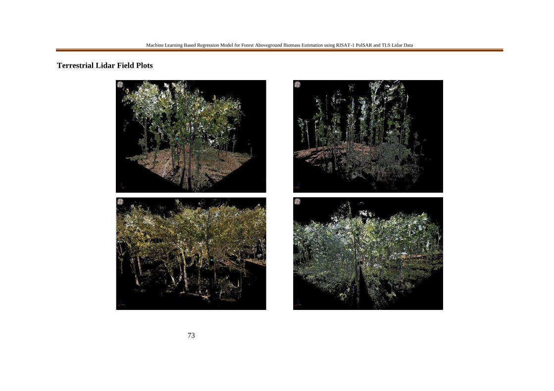
Machine Learning Based Regression Model for Forest Aboveground Biomass Estimation using RISAT-1 PolSAR and TLS Lidar Data
73
Terrestrial Lidar Field Plots

Machine Learning Based Regression Model for Forest Aboveground Biomass Estimation using RISAT-1 PolSAR and TLS Lidar Data
74

Machine Learning Based Regression Model for Forest Aboveground Biomass Estimation using RISAT-1 PolSAR and TLS Lidar Data
75

Machine Learning Based Regression Model for Forest Aboveground Biomass Estimation using RISAT-1 PolSAR and TLS Lidar Data
76

Machine Learning Based Regression Model for Forest Aboveground Biomass Estimation using RISAT-1 PolSAR and TLS Lidar Data
77
Field Data
TLS
Plot
Lat Long Biomass (t/ha) Height(m)
Plot 1 30.36973 77.72696 312.9246 22.832
Plot 2 30.35173 77.72258 249.5476 25.797
Plot 3 30.36955 77.73597 263.59 28.567
Plot 4 30.33616 77.7676 396.0751598 28.989
Plot 5 30.34037 77.75648 482.35842 26.732
Plot 6 30.36685 77.7128 321.8269 24.367
Plot 7 30.35808 77.71675 329.7345 22.242
Plot 8 30.3802 77.70256 475.3704 22.405
Plot 9 30.42037 77.67141 441.696 24.435
Plot 10 30.39091 77.71485 401.2888333 27.093
Plot 11 30.39461 77.69461 364.8354 23.497
Plot 12 30.41927 77.68437 365.3131588 24.502
Plot 13 30.36557 77.71947 285.7895 22.04
Plot 14 30.37038 77.72997 407.9679866 27.26

Machine Learning Based Regression Model for Forest Aboveground Biomass Estimation using RISAT-1 PolSAR and TLS Lidar Data
78
Field Photos


