Machine Learning Approach For Credit Score Analysis v8 - Final

14

MACHINE LEARNING APPROACH FOR

CREDIT SCORE ANALYSIS: A CASE STUDY OF

PREDICTING MORTGAGE LOAN DEFAULTS

Mohamed Hani AbdElHamid Mohamed Tawfik ElMasry

Submitted in partial fulfilment of the requirements for the degree of Statistics and Information Management specialized in Risk Management and Analysis

- 1 -

NOVA Information Management School

Instituto Superior de Estatística e Gestão de Informação

Universidade Nova de Lisboa

MACHINE LEARNING APPROACH FOR CREDIT SCORE ANALYSIS: A CASE STUDY OF PREDICTING

MORTGAGE LOAN DEFAULTS

by

Mohamed Hani AbdElHamid Mohamed Tawfik ElMasry Submitted in partial fulfilment of the requirements for the degree of Statistics and Information Management specialized in Risk Management and Analysis Supervisor: Professor Dr. Jorge Miguel Ventura Bravo

-----------------------------------------------------------

March 2019

- 2 -

Table of Contents LIST OF TABLES ...................................................................................................................................... - 4 -

LIST OF FIGURES .................................................................................................................................... - 5 -

LIST OF GRAPHS ..................................................................................................................................... - 6 -

ABSTRACT ................................................................................................................................................ - 7 -

RESUMO .................................................................................................................................................... - 8 -

1. INTRODUCTION .......................................................................................................................... - 9 -

1.1. PURPOSE .................................................................................................................................... - 12 -

1.2. THESIS OUTLINE ...................................................................................................................... - 12 -

2. LITERATURE REVIEW ............................................................................................................ - 13 -

2.1. A GLIMPSE FROM PARALLEL STUDIES ............................................................................. - 13 -

2.2. RESULTS FROM RELATED WORK ....................................................................................... - 14 -

3. MODELS PRESENTATION ....................................................................................................... - 16 -

3.1. ENSEMBLE ................................................................................................................................. - 16 -

3.1.1. STACKING .................................................................................................................................. - 20 -

3.2. PREDICTION MODELS ............................................................................................................ - 21 -

3.2.1. LOGISTIC REGRESSION ......................................................................................................... - 21 -

3.2.2. DECISION TREE ........................................................................................................................ - 22 -

3.2.3. RANDOM FOREST .................................................................................................................... - 23 -

3.2.4. K-NEAREST NEIGHBORS (KNN) ............................................................................................ - 24 -

3.2.5. SUPPORT VECTOR MACHINE (SVM) ................................................................................... - 24 -

3.2.6. MULTIPLE IMPUTATION BY CHAINED EQUATIONS (MICE) ... ...................................... - 25 -

3.3. EVALUATION CRITERIA ........................................................................................................ - 26 -

4. DATASET PROPERTIES ........................................................................................................... - 30 -

4.1. DATA DICTIONARY ................................................................................................................. - 30 -

4.1.1. ORIGINATION DATA................................................................................................................ - 31 -

4.1.2. PERFORMANCE DATA ............................................................................................................ - 34 -

4.2. EXPLORATORY ANALYSIS .................................................................................................... - 37 -

4.3. DATA WRANGLING .................................................................................................................. - 38 -

4.3.1. FEATURE IMPORTANCE ......................................................................................................... - 39 -

4.3.2. FEATURE ENGINEERING ....................................................................................................... - 40 -

4.3.3. MISSING OBSERVATIONS ...................................................................................................... - 41 -

4.4. DATA IMBALANCE ................................................................................................................... - 43 -

5. MODELLING .............................................................................................................................. - 45 -

- 3 -

5.1. BENCHMARK MODEL ............................................................................................................. - 45 -

5.2. ENSEMBLE TECHNIQUE ......................................................................................................... - 47 -

6. RESULTS ..................................................................................................................................... - 50 -

7. CONCLUSION ............................................................................................................................ - 53 -

8. REFERENCES ............................................................................................................................. - 55 -

- 4 -

List of Tables

TABLE 1:RESULTS FROM RELATED WORK ................................................................................... - 15 -

TABLE 2: AVERAGING EXAMPLE ..................................................................................................... - 17 -

TABLE 3: VOTING EXAMPLE ............................................................................................................. - 17 -

TABLE 4: CORRECTNESS OF PREDICTIONS PERFORMANCE MEA SURE ............................... - 26 -

TABLE 5: ACCURACY OF PROBABILITY PREDICTIONS PERFOR MANCE MEASURE .......... - 27 -

TABLE 6: DISCRIMINATORY ABILITY PERFORMANCE MEASURE ......................................... - 27 -

TABLE 7:CONTINGENCY TABLE OF BINARY CLASSIFICATION ............................................... - 28 -

TABLE 8: ORIGINATION FILE, DATA DICTIONARY ........ ............................................................. - 31 -

TABLE 9: PERFORMANCE FILE, DATA DICTIONARY ........ .......................................................... - 34 -

TABLE 10:ACCURACY RATE FOR LOGISTIC REGRESSION .... ................................................... - 46 -

TABLE 11: ACCURACY RATE FOR LEVEL ONE CLASSIFIERS . .................................................. - 49 -

- 5 -

List of Figures

FIGURE 1: STACKING ENSEMBLE .................................................................................................... - 11 -

FIGURE 2:A COMMON ENSEMBLE ARCHITECTURE ........... ........................................................ - 17 -

FIGURE 3:A GENERAL BOOSTING PROCEDURE ........................................................................... - 18 -

FIGURE 4:THE BAGGING ALGORITHM .................... ....................................................................... - 19 -

FIGURE 5:A GENERAL STACKING PROCEDURE ........................................................................... - 20 -

FIGURE 6:SIMPLE EXAMPLE OF A DECISION TREE ........ ............................................................ - 23 -

FIGURE 7:ILLUSTRATES HOW TO CLASSIFY AN INSTANCE BY A 3-NEAREST NEIGHBOR CLASSIFIER ............................................................................................................................................ - 24 -

FIGURE 8:THE MARGIN MAXIMIZATION IN SVMS .......... ............................................................ - 25 -

FIGURE 9: THREE TYPES OF PERFORMANCE MEASURE ........................................................... - 26 -

FIGURE 10: ENSEMBLE METHODOLOGY ....................................................................................... - 48 -

- 6 -

List of Graphs

GRAPH 1: ROC SPACE .......................................................................................................................... - 29 -

GRAPH 2:DEFAULT RATE BY YEAR ACROSS OUR DATASET ... ................................................. - 37 -

GRAPH 3:DEFAULT RATE BY ORIGINATION YEAR .......... ........................................................... - 38 -

GRAPH 4:MISSING VALUES VISUALIZATION .............. .................................................................. - 42 -

GRAPH 5:MISSING VALUES VISUALIZATION AFTER ZERO-VAR IABLES ELIMINATION ... - 43 -

GRAPH 6: ROC CURVE BASED ON THE ELIMINATED NAS MODE L ......................................... - 46 -

GRAPH 7: ROC CURVE BASED ON THE IMPUTED NAS MODEL . ............................................... - 47 -

GRAPH 8: MODELS’ ACCURACY ....................................................................................................... - 50 -

GRAPH 9:ROC CURVE OF ENSEMBLE MODEL .............................................................................. - 51 -

GRAPH 10:ACCURACY COMPARISON OF STACKING ENSEMBLE . ........................................... - 52 -

- 7 -

NOVA Information Management School Instituto Superior de Estatística e Gestão de Informação


Master of Statistics and Information Management Specialized in Risk Management and Analysis

MACHINE LEARNING APPROACH FOR CREDIT SCORE ANALYSIS: A CASE STUDY OF PREDICTING MORTGAGE LOAN DEFAULTS

By Mohamed Hani ElMasry

Abstract

To effectively manage credit score analysis, financial institutions instigated techniques and models that

are mainly designed for the purpose of improving the process assessing creditworthiness during the

credit evaluation process. The foremost objective is to discriminate their clients – borrowers – to fall

either in the non-defaulter group, that is more likely to pay their financial obligations, or the defaulter

one which has a higher probability of failing to pay their debts. In this paper, we devote to use machine

learning models in the prediction of mortgage defaults. This study employs various single classification

machine learning methodologies including Logistic Regression, Classification and Regression Trees,

Random Forest, K-Nearest Neighbors, and Support Vector Machine. To further improve the predictive

power, a meta-algorithm ensemble approach – stacking – will be introduced to combine the outputs –

probabilities – of the afore mentioned methods. The sample for this study is solely based on the publicly

provided dataset by Freddie Mac. By modelling this approach, we achieve an improvement in the model

predictability performance. We then compare the performance of each model, and the meta-learner, by

plotting the ROC Curve and computing the AUC rate. This study is an extension of various preceding

studies that used different techniques to further enhance the model predictivity. Finally, our results are

compared with work from different authors.

Key words:

Credit Scoring, Machine Learning, Predictive Modelling, Stacking Ensemble, Freddie Mac, Logistic

Regression, Decision Tree, Random Forest, K-Nearest Neighbors, Support Vector Machine

- 8 -

NOVA Information Management School Instituto Superior de Estatística e Gestão de Informação


Master of Statistics and Information Management Specialized in Risk Management and Analysis

MACHINE LEARNING APPROACH FOR CREDIT SCORE ANALYSIS: A CASE STUDY OF PREDICTING MORTGAGE LOAN DEFAULTS

By Mohamed Hani ElMasry

Resumo

Para gerir com eficácia o risco de crédito, as instituições financeiras desenvolveram técnicas e modelos

para melhorar o processo de avaliação da qualidade de crédito durante o processo de avaliação de

propostas de crédito. O objetivo final é o de classificar os seus clientes - tomadores de empréstimos -

entre aqueles que tem maior probabilidade de cumprir as suas obrigações financeiras, e os potenciais

incumpridores que têm maior probabilidade de entrar em default. Nesta dissertação usamos diferentes

metodologias de machine learning, incluindo Regressão Logistica, Classification and Regression Trees,

Random Forest, K-Nearest Neighbors, e Support Vector Machine na previsão do risco de default em

crédito à habitação. Para melhorar o poder preditivo dos modelos, introduzimos a abordagem do

conjunto de meta-algoritmos - stacking - para combinar as saídas - probabilidades - dos métodos acima

mencionados. A amostra deste estudo é baseada exclusivamente no conjunto de dados fornecido

publicamente pela Freddie Mac. Avaliamos em que medida a utilização destes modelos permite uma

melhoria no desempenho preditivo. Em seguida, comparamos o desempenho de cada modelo e a

stacking approach através da Curva ROC e do cálculo da AUC. Este estudo é uma extensão de vários

estudos anteriores que usaram diferentes técnicas para melhorar a capacidade preditiva dos modelos.

Palavras-chave:

Scoring de crédito, Machine Learning, Predictive Modelling, Stacking Ensemble, Freddie Mac,

Regressão logística, Decision Tree, Random Forest, K-Nearest Neighbors, Support Vector Machine

- 9 -

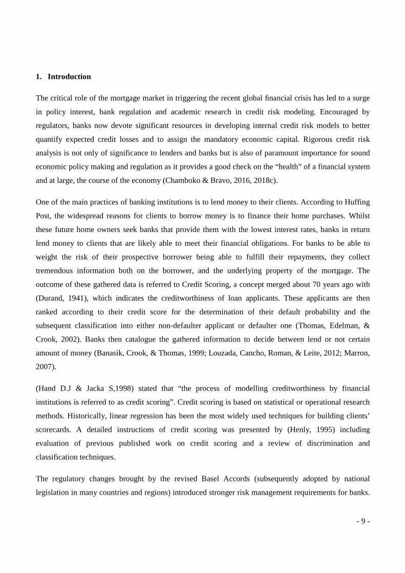
1. Introduction

The critical role of the mortgage market in triggering the recent global financial crisis has led to a surge

in policy interest, bank regulation and academic research in credit risk modeling. Encouraged by

regulators, banks now devote significant resources in developing internal credit risk models to better

quantify expected credit losses and to assign the mandatory economic capital. Rigorous credit risk

analysis is not only of significance to lenders and banks but is also of paramount importance for sound

economic policy making and regulation as it provides a good check on the “health” of a financial system

and at large, the course of the economy (Chamboko & Bravo, 2016, 2018c).

One of the main practices of banking institutions is to lend money to their clients. According to Huffing

Post, the widespread reasons for clients to borrow money is to finance their home purchases. Whilst

these future home owners seek banks that provide them with the lowest interest rates, banks in return

lend money to clients that are likely able to meet their financial obligations. For banks to be able to

weight the risk of their prospective borrower being able to fulfill their repayments, they collect

tremendous information both on the borrower, and the underlying property of the mortgage. The

outcome of these gathered data is referred to Credit Scoring, a concept merged about 70 years ago with

(Durand, 1941), which indicates the creditworthiness of loan applicants. These applicants are then

ranked according to their credit score for the determination of their default probability and the

subsequent classification into either non-defaulter applicant or defaulter one (Thomas, Edelman, &

Crook, 2002). Banks then catalogue the gathered information to decide between lend or not certain

amount of money (Banasik, Crook, & Thomas, 1999; Louzada, Cancho, Roman, & Leite, 2012; Marron,

2007).

(Hand D.J & Jacka S,1998) stated that “the process of modelling creditworthiness by financial

institutions is referred to as credit scoring”. Credit scoring is based on statistical or operational research

methods. Historically, linear regression has been the most widely used techniques for building clients’

scorecards. A detailed instructions of credit scoring was presented by (Henly, 1995) including

evaluation of previous published work on credit scoring and a review of discrimination and

classification techniques.

The regulatory changes brought by the revised Basel Accords (subsequently adopted by national

legislation in many countries and regions) introduced stronger risk management requirements for banks.

- 10 -

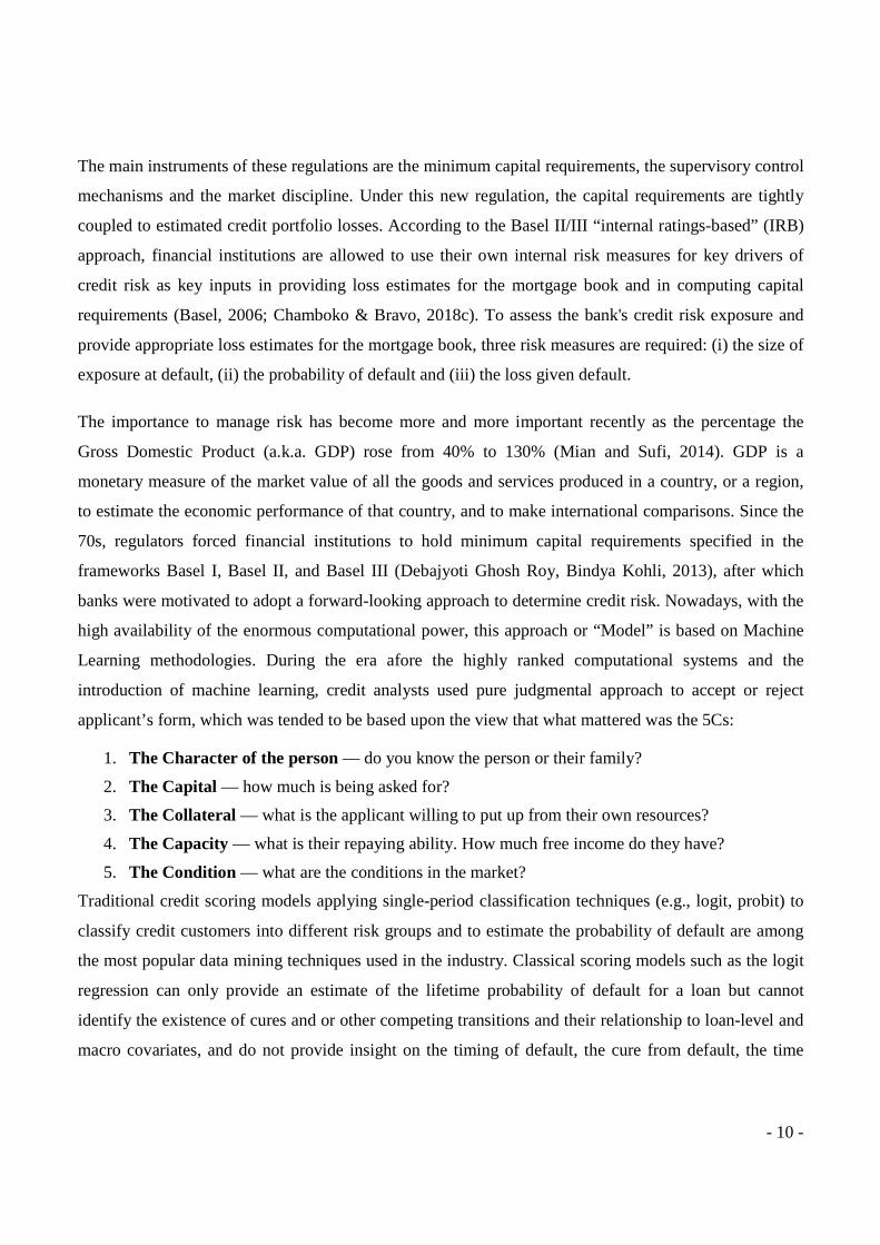
The main instruments of these regulations are the minimum capital requirements, the supervisory control

mechanisms and the market discipline. Under this new regulation, the capital requirements are tightly

coupled to estimated credit portfolio losses. According to the Basel II/III “internal ratings-based” (IRB)

approach, financial institutions are allowed to use their own internal risk measures for key drivers of

credit risk as key inputs in providing loss estimates for the mortgage book and in computing capital

requirements (Basel, 2006; Chamboko & Bravo, 2018c). To assess the bank's credit risk exposure and

provide appropriate loss estimates for the mortgage book, three risk measures are required: (i) the size of

exposure at default, (ii) the probability of default and (iii) the loss given default.

The importance to manage risk has become more and more important recently as the percentage the

Gross Domestic Product (a.k.a. GDP) rose from 40% to 130% (Mian and Sufi, 2014). GDP is a

monetary measure of the market value of all the goods and services produced in a country, or a region,

to estimate the economic performance of that country, and to make international comparisons. Since the

70s, regulators forced financial institutions to hold minimum capital requirements specified in the

frameworks Basel I, Basel II, and Basel III (Debajyoti Ghosh Roy, Bindya Kohli, 2013), after which

banks were motivated to adopt a forward-looking approach to determine credit risk. Nowadays, with the

high availability of the enormous computational power, this approach or “Model” is based on Machine

Learning methodologies. During the era afore the highly ranked computational systems and the

introduction of machine learning, credit analysts used pure judgmental approach to accept or reject

applicant’s form, which was tended to be based upon the view that what mattered was the 5Cs:

1. The Character of the person — do you know the person or their family?

2. The Capital — how much is being asked for?

3. The Collateral — what is the applicant willing to put up from their own resources?

4. The Capacity — what is their repaying ability. How much free income do they have?

5. The Condition — what are the conditions in the market?

Traditional credit scoring models applying single-period classification techniques (e.g., logit, probit) to

classify credit customers into different risk groups and to estimate the probability of default are among

the most popular data mining techniques used in the industry. Classical scoring models such as the logit

regression can only provide an estimate of the lifetime probability of default for a loan but cannot

identify the existence of cures and or other competing transitions and their relationship to loan-level and

macro covariates, and do not provide insight on the timing of default, the cure from default, the time

- 11 -

since default and time to collateral repossession (Gaffney et al., 2014; Chamboko & Bravo, 2018a,b,c).

Nowadays, with the revolution of big data and its uncontroversial positive effect, banking institutions

use machine learning approach, which mainly refers to a set of algorithms designed to tackle

computationally intensive pattern-recognition problems in extremely large datasets. The widely used

ones are Bagging (Leo Breiman, 1996), Boosting (Schapire, Freund, Bartlett, & Lee, 1998), and recently

Stacking (Wolpert, 1992). These are called Ensemble methods (Dumitrescu et al. 2018).

Bagging and Boosting aim at improving the predictive power of machine learning algorithms by using a

linear combination of predictions from many variants of this algorithm, through averaging or majority

vote, rather than individual model. Bagging is the application of the Bootstrap (Efron & Tibshirani,

1993) procedure to a high-variance machine learning algorithm, typically decision trees. Boosting uses

an iterative method, where it mainly learns from individuals that were misclassified in previous

iterations by giving them more weight so that in the next iteration the learner would focus more on them.

We will not dig any deeper in Bagging or Boosting in this paper, as we will be more focused on the

Stacking technique. For a review of Bagging and Boosting methods see (Bühlmann, 2012; Hastie,

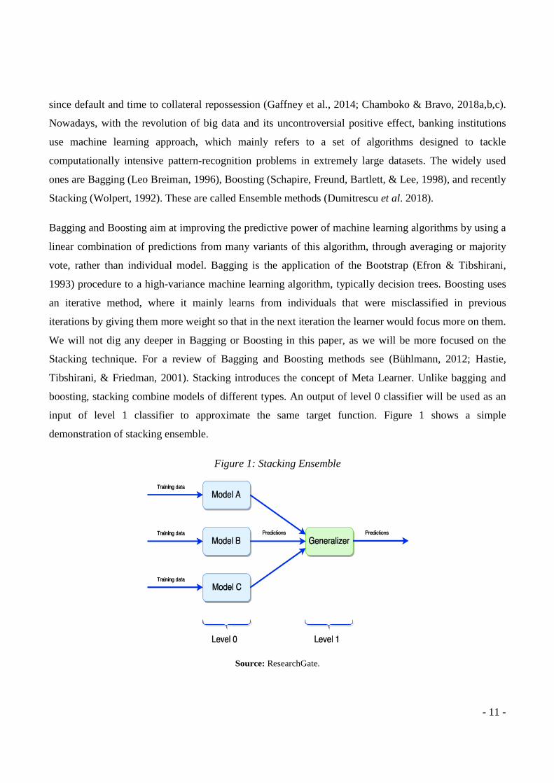
Tibshirani, & Friedman, 2001). Stacking introduces the concept of Meta Learner. Unlike bagging and

boosting, stacking combine models of different types. An output of level 0 classifier will be used as an

input of level 1 classifier to approximate the same target function. Figure 1 shows a simple

demonstration of stacking ensemble.

Figure 1: Stacking Ensemble

Source: ResearchGate.

- 12 -

1.1. Purpose

The novelty of this paper lies in making use of stacking ensemble (Smyth & Wolpert, 1998; Wolpert,

1992) in predicting the mortgage default. We use machine learning methods, such as Linear

Discriminate Analysis (LDA), Classification and Regression Trees (CART), Random Forest (RM), K-

Nearest Neighbors (KNN), and Support Vector Machine (SVM) as a level 0 classifier and use the output

as an input to Logistic Regression (LR) model. We shall examine and compare the output with a single

classifier output of the same level 1 model, logistic regression, via AUC and ROC curve. In this thesis,

we are using a data set provided by Freddie Mac. Freddie Mac is a government-sponsored enterprise that

plays a central role in the US housing finance system and at the start of their conservatorships held or

guaranteed about $5.2 trillion of home mortgage debt. The firm was often cited as a shining example of

public-private partnerships—that is, the harnessing of private capital to advance the social goal of

expanding homeownership (Frame, Fuster, Tracy, & Vickery, 2015).

1.2. Thesis Outline

The first section of the paper will introduce the credit risk modelling and highlight some of the

techniques previously used and wide grow of the data presence, which led to surfacing of the statistical

techniques. The second section will be the literature review and the model presentation. In the third

section, we will focus on the methodology used for the data preparation, where we will discuss “mice”

for missing data imputation, some feature selection techniques, and Stacking Ensemble. The third

section will also discuss the modelling technique that will be applied on the data. It is worthy to mention

that R-Studio was used throughout the entire pre-processing and modelling stages. The fourth section

will explore our dataset and highlight the relationship between the default rate and the available

variables. The fifth section will be applying the models to our dataset. The sixth section will highlight all

the outputs and discuss the accuracy of each model. The sixth and the final section will conclude our

work.

- 13 -

2. Literature Review

In this section, we provide a brief lookback on previous studies by various authors, we well as some of

their remarkable results.

2.1. A Glimpse from Parallel Studies

There are many studies developed, and still developing, in this subject. Various methodologies and

approaches were applied to increase the predictive power and the output accuracy level with the least

overfitting issue, yet, many models and methodologies remain uncovered and assorted questions remain

to be answered. (AlAmari, 2002) highlighted some of the questions regarding the optimal methods for

customer evaluations and the variables – features – that a credit analyst should include in assessing a

borrower’s application. He also extended his argument with more questions like “What is the best

statistical technique on the basis of the highest average correct classification rate or lowest

misclassification cost or other evaluation criteria?”. Some modelling cases follow around studies on this

area, (Hand, 2005) for example, used latent-variable technique to split the clients’ physiognomies into

primary characteristics (X) and behavioral characteristics (Y). Then the study summarizes them into

overall measure of credit consumer scores. Early research focused on determining the major factors in

determining default rates rather than building a predictive model to discriminate between the good client

and the bad one (non-defaulter and defaulter respectively). For example, (Vandell, 1978) hypothesis

stated that the ratio of loan value to the property value are the foremost variable.

Although application of machine learning in Finance is relatively new concept, yet, much research has

been conducted in that area. (Khandani, Kim, & Lo, 2010), (Butaru et al., 2016), (Fitzpatrick & Mues,

2016), (Jafar Hamid & Ahmed, 2016), (I. Brown & Mues, 2012), (Bolarinwa, 2017) and (Sealand, 2018)

employed machine learning in predicting loan default. Some of these studies used small datasets with

several thousand mortgages, while other used dataset of millions of mortgages. Models used include

logistic regression (single and multinomial), Naïve Bayes, Random Forest, Ensemble (Y. W. Zhou,

Zhong & Li, 2012)1, K-Nearest Neighborhood and Survival Analysis (Bellotti & Crook, 2009).

- 14 -

In (Bolarinwa, 2017) research, random forest performed extremely well with an accuracy of 95.68%,

and Naïve Bayes had the lowest accuracy of 70.74%. Worth mentioning that most published studies

compiled data from different sources such as employment rates and rent ratio data. (Sealand, 2018)

summarized the results from the top research studies carried that highlighted an AUC output of 99.42%,

95.64%, and 92.92% for (I. Brown & Mues, 2012), (Bolarinwa, 2017), and (Deng, 2016) respectively.

(Groot, 2016), (Deng, 2016), (Sealand, 2018) and (Bolarinwa, 2017) used either data from Freddie Mac,

or Fennie Mae.

When applying these machine learning techniques, all research followed (Koh, Tan & Goh, 2006)

illustration of the use of data mining techniques, the suggested model has five steps: defining the

objective, selecting variables, selecting sample and collecting data, selecting modelling tools and

constructing models, validating and assessing models. Feature reduction was another technique

introduced in the financial world by (Azam, Danish & Akbar, 2012) who evaluated the significance of

loan applicant socioeconomic attributes on personal loan decision in banks using descriptive statistics

and logistic regression, which identified that out of six independent variables only three variables

(region, residence status and year with the current organization) have significant impact on personal loan

decision.

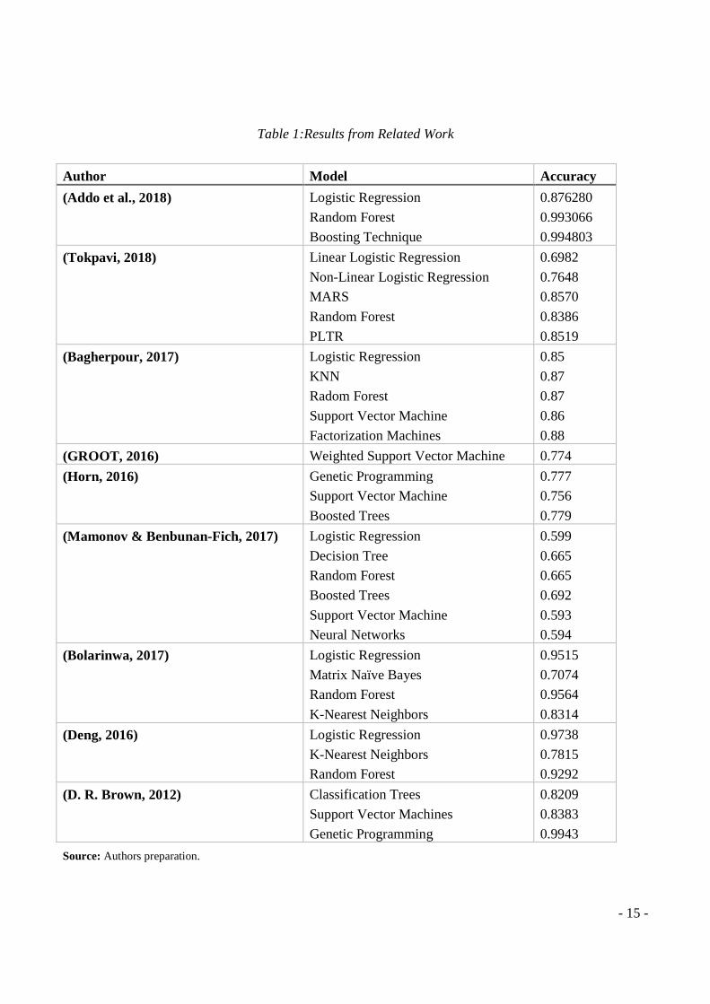
2.2. Results from Related Work

Results from related previous work, such as that of (Addo, Guegan, & Hassani, 2018), (Tokpavi, 2018),

(Bagherpour, 2017), (GROOT, 2016), (Horn, 2016), (Mamonov & Benbunan-Fich, 2017), (Bolarinwa,

2017), (Deng, 2016), and (D. R. Brown, 2012) are included in Table 1.

- 15 -

Table 1:Results from Related Work

Author Model Accuracy

(Addo et al., 2018) Logistic Regression

Random Forest

Boosting Technique

0.876280

0.993066

0.994803

(Tokpavi, 2018) Linear Logistic Regression

Non-Linear Logistic Regression

MARS

Random Forest

PLTR

0.6982

0.7648

0.8570

0.8386

0.8519

(Bagherpour, 2017) Logistic Regression

KNN

Radom Forest

Support Vector Machine

Factorization Machines

0.85

0.87

0.87

0.86

0.88

(GROOT, 2016) Weighted Support Vector Machine 0.774

(Horn, 2016) Genetic Programming


Boosted Trees

0.777

0.756

0.779

(Mamonov & Benbunan-Fich, 2017) Logistic Regression

Decision Tree

Random Forest

Boosted Trees


Neural Networks

0.599

0.665

0.665

0.692

0.593

0.594

(Bolarinwa, 2017) Logistic Regression

Matrix Naïve Bayes

Random Forest

K-Nearest Neighbors

0.9515

0.7074

0.9564

0.8314

(Deng, 2016) Logistic Regression

K-Nearest Neighbors

Random Forest

0.9738

0.7815

0.9292

(D. R. Brown, 2012) Classification Trees

Support Vector Machines

Genetic Programming

0.8209

0.8383

0.9943

Source: Authors preparation.

- 16 -

3. Models Presentation

In this section we aim to present the differences between the Ensemble techniques and discuss the

prediction models used in our study.

3.1. Ensemble

Ensemble methods that train multiple learners (the learned model can be called a hypothesis) and then

combine them for use, with Boosting and Bagging as representatives, are a kind of state-of-the art

learning approach. Ensemble methods train multiple learners to solve the same problem.

Contrary to ordinary learning approaches which try to construct one learner from training data, ensemble

methods try to construct a set of learners and combine them. Ensemble learning is also called

committee-based learning, or learning multiple classifier systems (Z.-H. Zhou, 2012). Ensemble is

merely a technique that boost the accuracy of weak learners (also referred to as base learners) to strong

learners, which can make very accurate predictions. It combines two or more algorithms of similar or

dissimilar types called base learners. This makes a more robust system, which incorporates the

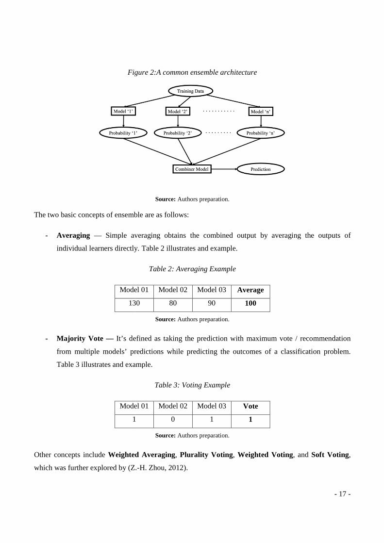
predictions from all the base learners to get our final “accurate” and less likely biased decision. Figure 2

shows a common ensemble architecture.

There are three threads of early contributions that led to the current area of ensemble methods; that is,

combining classifiers, ensembles of weak learners and mixture of experts.

- Combining classifiers was mostly studied in the pattern recognition community. Researchers in

this thread generally work on strong classifiers and try to design powerful combining rules to get

stronger combined classifiers.

- Ensembles of weak learners was mostly studied in the machine learning community.

Researches in this field often work on weak learners and try to design powerful algorithms to

boost the performance from weak to strong.

- Mixture of experts was mostly studied in the neural networks’ community. Researchers generally consider a divide-and-conquer strategy, try to learn a mixture of parametric models jointly and use combining rules to get an overall solution.

Figure

The two basic concepts of ensemble are as follows:

- Averaging — Simple averaging obtains the combined output by averaging the outputs of

individual learners directly.

Model 01

130

- Majority Vote — It’s defined as taking the prediction with maximum vote / recommendation

from multiple models’ predictions while predicting the outcomes of a classification problem.

Table 3 illustrates and example.

Model 01

1

Other concepts include Weighted Averaging

which was further explored by (Z.

Figure 2:A common ensemble architecture


f ensemble are as follows:

Simple averaging obtains the combined output by averaging the outputs of

individual learners directly. Table 2 illustrates and example.

Table 2: Averaging Example

Model 01 Model 02 Model 03 Average

130 80 90 100


It’s defined as taking the prediction with maximum vote / recommendation


example.

Table 3: Voting Example

Model 01 Model 02 Model 03 Vote

1 0 1 1


Weighted Averaging, Plurality Voting , Weighted Voting

(Z.-H. Zhou, 2012).

- 17 -

Simple averaging obtains the combined output by averaging the outputs of

It’s defined as taking the prediction with maximum vote / recommendation


Weighted Voting, and Soft Voting,

Boosting and Bagging

There are two paradigms of ensemble methods, that is, sequential ensemble methods, wh

learners are generated sequentially, with Boosting as a representative, and parallel ensemble methods

where the base learners are generated in parallel, with Bagging as a representative.

The basic motivation of sequential methods is to exploit

the overall performance can be boosted in a residual

of parallel ensemble methods is to exploit the independence between the base learners, since the error

can be reduced dramatically by combining independent base learners.

Boosting

Boosting refers to boosting performance of weak models. It involves the first algorithm is trained on the

entire training data and the subsequent algorithms are built by fitting the

thus giving higher weight to those observations that were poorly predicted by the previous model.

Figure

Source: Ensemble Methods Foundations and Algorithms

The general boosting procedure is quite simple. Suppose the weak learner will work on any data

distribution it is given and take the binary classification task as an example; that is, we are trying to

classify instances as positive and negative. The training instances in space X are drawn i.i.d. from

distribution D, and the ground-truth function is

X2 and X3, each takes 1/3 amount of the distribution, and a learner working by random guess has 50%

There are two paradigms of ensemble methods, that is, sequential ensemble methods, wh



The basic motivation of sequential methods is to exploit the dependence between the base learners, since

the overall performance can be boosted in a residual-decreasing way. Meanwhile, the basic motivation


be reduced dramatically by combining independent base learners.


entire training data and the subsequent algorithms are built by fitting the residuals of the first algorithm,


Figure 3:A general boosting procedure

Ensemble Methods Foundations and Algorithms (Z.-H. Zhou, 2012)


is given and take the binary classification task as an example; that is, we are trying to


truth function is ‘f’. Suppose the space X is composed of three parts

, each takes 1/3 amount of the distribution, and a learner working by random guess has 50%

- 18 -

There are two paradigms of ensemble methods, that is, sequential ensemble methods, where the base



the dependence between the base learners, since

decreasing way. Meanwhile, the basic motivation



residuals of the first algorithm,


H. Zhou, 2012).


is given and take the binary classification task as an example; that is, we are trying to


e space X is composed of three parts X1,

, each takes 1/3 amount of the distribution, and a learner working by random guess has 50%

classification error on this problem. We want to get an accurate (e.g., zero error) classifier on the

problem, but we are unlucky and only have a weak classifier at hand, which only has correct

classifications in spaces X1 and X

Let’s denote this weak classifier as

The idea of boosting is to correct the mistakes made by

from D, which makes the mistakes of

we can train a classifier h2 from D

which has corrected classifications in

and h2 in an appropriate way, the combined classifier will have correct classifications in

some errors in X2 and X3. Again, we derive a new dist

classifier more evident, and train a classifier

classifications in X2 and X3. Then, by combining

space of X1, X2 and X3, at least two classifiers make correct classifications.

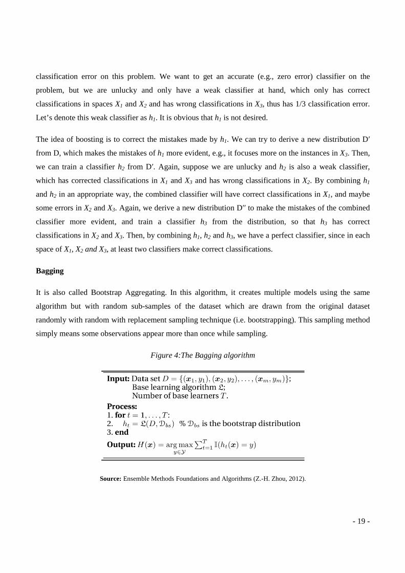
Bagging

It is also called Bootstrap Aggregating. In this algorithm, it creates multiple models using the same

algorithm but with random sub-

randomly with random with replacement sampling technique (i.e. bootstrapping). This sampling method

simply means some observations appear more than once while sampling.



we are unlucky and only have a weak classifier at hand, which only has correct

X2 and has wrong classifications in X3, thus has 1/3 classification error.

Let’s denote this weak classifier as h1. It is obvious that h1 is not desired.

The idea of boosting is to correct the mistakes made by h1. We can try to derive a new distribution D

from D, which makes the mistakes of h1 more evident, e.g., it focuses more on the instances in

from D′. Again, suppose we are unlucky and h2

classifications in X1 and X3 and has wrong classifications in

the combined classifier will have correct classifications in

Again, we derive a new distribution D′′ to make the mistakes of the combined

classifier more evident, and train a classifier h3 from the distribution, so that

. Then, by combining h1, h2 and h3, we have a perfect classifier, since in each

, at least two classifiers make correct classifications.


-samples of the dataset which are drawn


simply means some observations appear more than once while sampling.

Figure 4:The Bagging algorithm


- 19 -


we are unlucky and only have a weak classifier at hand, which only has correct

, thus has 1/3 classification error.

. We can try to derive a new distribution D′

more evident, e.g., it focuses more on the instances in X3. Then,

2 is also a weak classifier,

and has wrong classifications in X2. By combining h1

the combined classifier will have correct classifications in X1, and maybe

′′ to make the mistakes of the combined

from the distribution, so that h3 has correct

, we have a perfect classifier, since in each


from the original dataset


H. Zhou, 2012).

After fitting several models on different samples, th

weighted average or a voting method.

The bagging and boosting algorithms are suitable means to increase efficiency of

algorithms, however, the loss of simplicity of this classification sche

disadvantage (Machova, Puszta, Barcak, & Bednar, 2006)

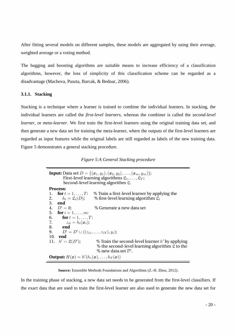
3.1.1. Stacking

Stacking is a technique where a learner is trained to combine the individual

individual learners are called the

learner, or meta-learner. We first train the first

then generate a new data set for training the meta

regarded as input features while the original labels are still regarded as labels of the new training data.

Figure 5 demonstrates a general stacking procedure.

F


In the training phase of stacking, a new data set needs to be generated from the first

the exact data that are used to train the first

After fitting several models on different samples, these models are aggregated by using their average,

method.

The bagging and boosting algorithms are suitable means to increase efficiency of

algorithms, however, the loss of simplicity of this classification scheme can be

(Machova, Puszta, Barcak, & Bednar, 2006).

is a technique where a learner is trained to combine the individual

individual learners are called the first-level learners, whereas the combiner is called the

We first train the first-level learners using the original training data set, and

new data set for training the meta-learner, where the outputs of the first


Figure 5 demonstrates a general stacking procedure.

Figure 5:A General Stacking procedure


In the training phase of stacking, a new data set needs to be generated from the first

the exact data that are used to train the first-level learner are also used to generate the new data set for

- 20 -

aggregated by using their average,

The bagging and boosting algorithms are suitable means to increase efficiency of a classification

me can be regarded as a

is a technique where a learner is trained to combine the individual learners. In stacking, the

, whereas the combiner is called the second-level

level learners using the original training data set, and

learner, where the outputs of the first-level learners are


hou, 2012).

In the training phase of stacking, a new data set needs to be generated from the first-level classifiers. If

level learner are also used to generate the new data set for

- 21 -

training the second-level learner, there will be a high risk of overfitting. Hence, it is suggested that the

instances used for generating the new data set are excluded from the training examples for the first-level

learners, and a cross- validation or leave-one-out procedure is often recommended.

Generally stacking proved success in many different applications. (Leo Breiman, 1996) demonstrated

the success of stacked regression, where he used linear regression models with different numbers of

variables as the first-level learners, and least-square linear regression model as the second-level learner

under the constraint that all regression coefficients are non-negative. This non-negativity constraint was

found to be crucial to guarantee that the performance of the stacked ensemble would be better than

selecting the single best learner.

Since many previous studies were conducted using Boosting and Bagging, in our paper we will be

implementing stacking ensemble technique to fit our model.

3.2. Prediction Models

In this section, we will briefly explore the prediction models used in this paper. Models explored include

Logistic Regression, Decision Tree, Random Forest, K-Nearest Neighbors, and Support Vector

Machine.

3.2.1. Logistic Regression

Logistic Regression model (Cox, 1958) is a statistical method utilized in machine learning to assess the

relationship between a dependent categorical variable (output) and one or more independent variables

(predictors) by employing a logistic function to evaluate the probabilities. Logistic Regression can be

binary (output variable has two classes), multinomial (output variable has more than two classes) or

ordinal (Bolarinwa, 2017). In our study we only use the linear output as we are only discriminate

between default and non-default loans.

The logistic function is given by formula (1):

- 22 -

�� =1

1 + �� (1)

where f(x), in this scope, represents the probability of an output variable (two classes: 0 or 1), �0 is the

linear regression intercept and �1 is the multiplication of the regression coefficient by x value of the

independent variable. In our application, the output variable with the value 1 represents the probability

of loan status being default and 0 is the probability of loan status equaling paying. This information can

be represented in a form of a logistic equation as shown in formula (2):

� = �� = 1� =1

1 + ��(��⋯��) (2)

where k is the number of independent variables. Therefore, the logistic regression formula for default

loans becomes:

�(�)

1 − �(�)= ��(��⋯��) (3)

Concluding that the formula for non-default loans will simply be 1-p.

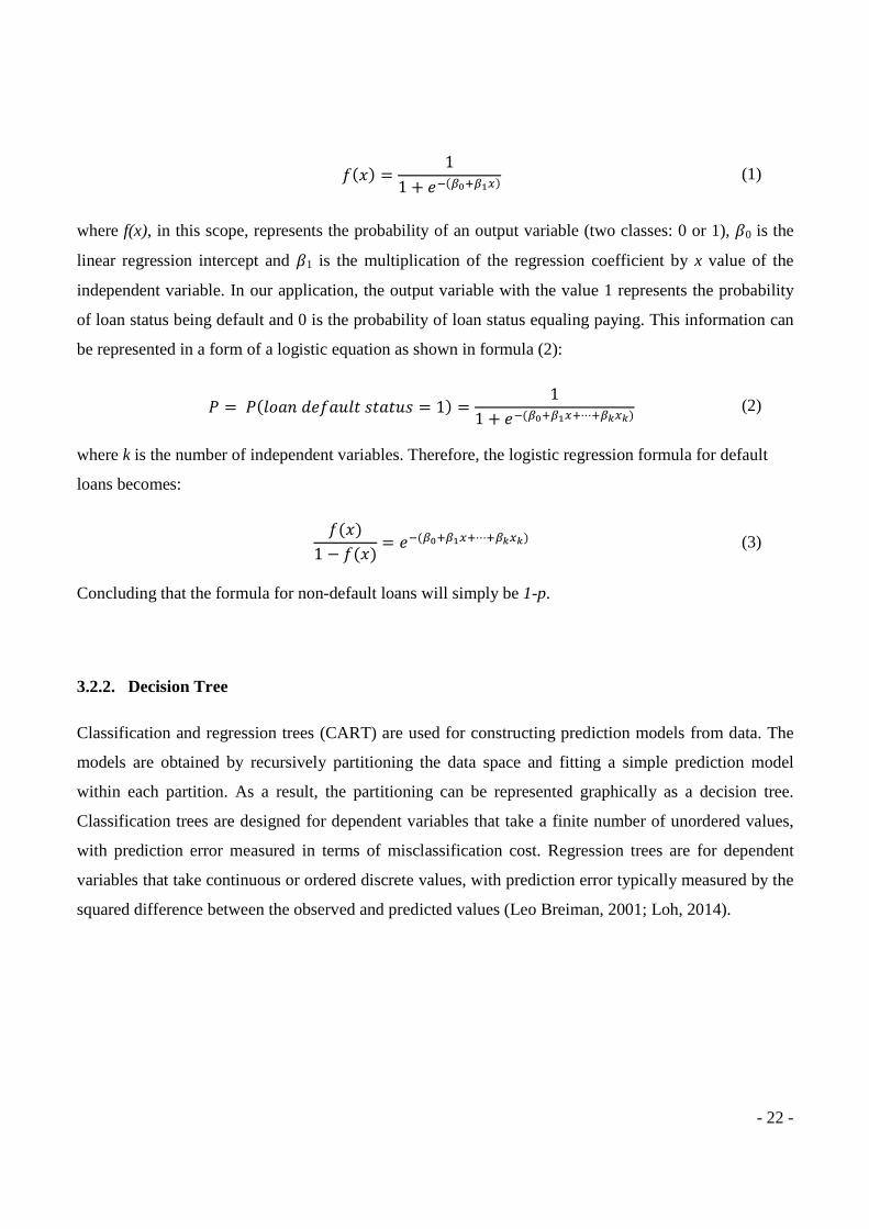
3.2.2. Decision Tree

Classification and regression trees (CART) are used for constructing prediction models from data. The

models are obtained by recursively partitioning the data space and fitting a simple prediction model

within each partition. As a result, the partitioning can be represented graphically as a decision tree.

Classification trees are designed for dependent variables that take a finite number of unordered values,

with prediction error measured in terms of misclassification cost. Regression trees are for dependent

variables that take continuous or ordered discrete values, with prediction error typically measured by the

squared difference between the observed and predicted values (Leo Breiman, 2001; Loh, 2014).

Figure


One problem with decision trees is that features with a

their relevance to classification. The information gain split would be quite large in this case. This is

where C4.5 algorithm (Quinlan, 1992)

criterion by employing gain ratios, which is simply a variant of the information gain criterion, taking

normalization on the number of feature values. In real

selected as the split. Cart (L Breiman, Friedman, Olshen & Stone, 1984)

algorithm, which uses Gini index for selecting the split

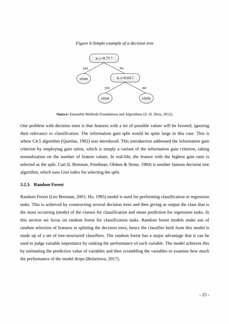
3.2.3. Random Forest

Random Forest (Leo Breiman, 2001; Ho, 1995)

tasks. This is achieved by constructing several decision trees and then giving as output the class that is

the most occurring (mode) of the classes for classification and mean prediction for regression tasks. In

this section we focus on random forest for classification tasks. Random

random selection of features in splitting the decision trees, hence the classifier built from this model is

made up of a set of tree-structured classifiers.

used to judge variable importance by ranking the performance of each variable. The model achieves this

by estimating the predictive value of variables and then scrambling the variables to examine how much

the performance of the model drops

Figure 6:Simple example of a decision tree


One problem with decision trees is that features with a lot of possible values will be favored, ignoring


(Quinlan, 1992) was introduced. This introduction addressed the information gain


n the number of feature values. In real-life, the feature with the highest gain ratio is

(L Breiman, Friedman, Olshen & Stone, 1984) is another famous decision tree

ses Gini index for selecting the split.

(Leo Breiman, 2001; Ho, 1995) model is used for performing classification or regression

onstructing several decision trees and then giving as output the class that is


this section we focus on random forest for classification tasks. Random forest models make use of


structured classifiers. The random forest has a major advantage that it can be

able importance by ranking the performance of each variable. The model achieves this


the performance of the model drops (Bolarinwa, 2017).

- 23 -

H. Zhou, 2012).

lot of possible values will be favored, ignoring


introduced. This introduction addressed the information gain


life, the feature with the highest gain ratio is

is another famous decision tree

for performing classification or regression

onstructing several decision trees and then giving as output the class that is


forest models make use of


The random forest has a major advantage that it can be

able importance by ranking the performance of each variable. The model achieves this


- 24 -

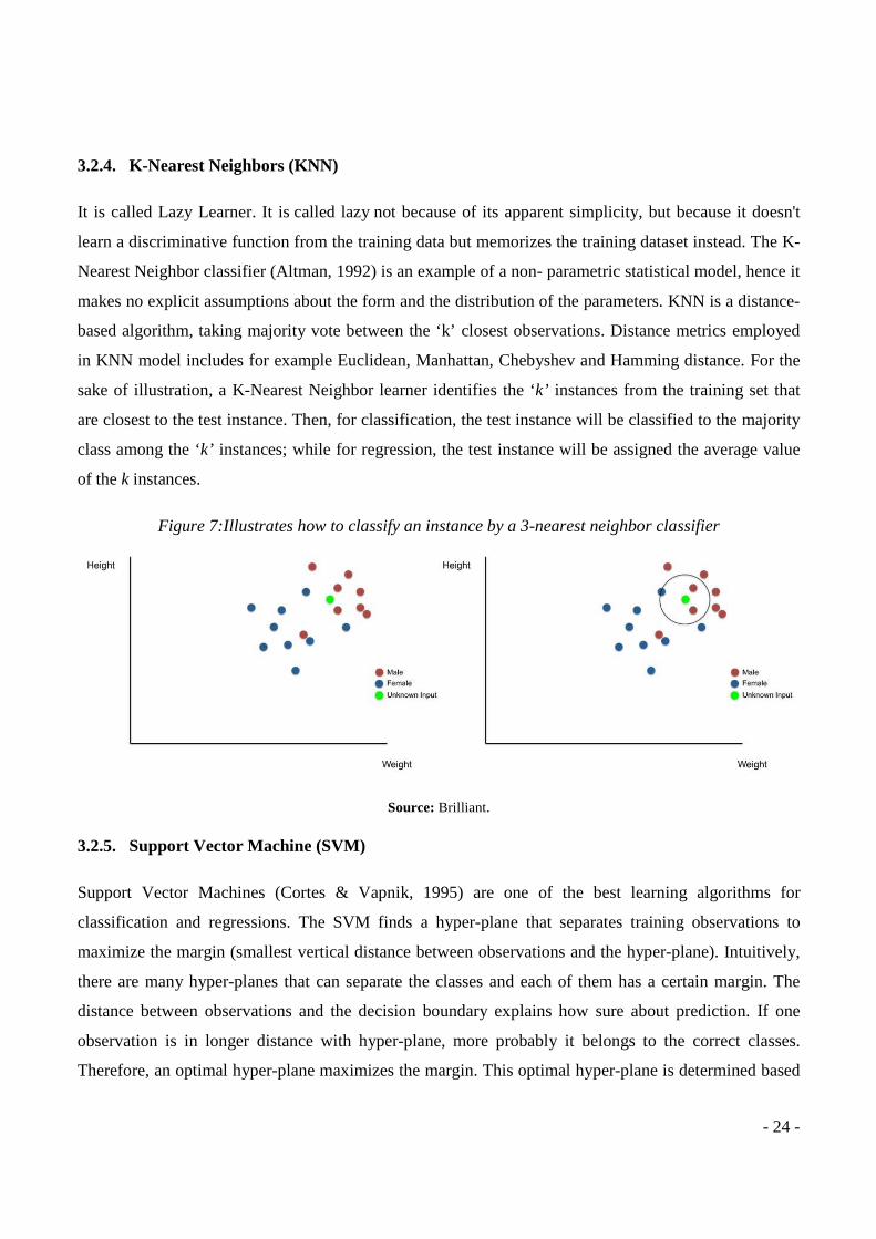
3.2.4. K-Nearest Neighbors (KNN)

It is called Lazy Learner. It is called lazy not because of its apparent simplicity, but because it doesn't

learn a discriminative function from the training data but memorizes the training dataset instead. The K-

Nearest Neighbor classifier (Altman, 1992) is an example of a nonparametric statistical model, hence it

makes no explicit assumptions about the form and the distribution of the parameters. KNN is a distance-

based algorithm, taking majority vote between the ‘k’ closest observations. Distance metrics employed

in KNN model includes for example Euclidean, Manhattan, Chebyshev and Hamming distance. For the

sake of illustration, a K-Nearest Neighbor learner identifies the ‘k’ instances from the training set that

are closest to the test instance. Then, for classification, the test instance will be classified to the majority

class among the ‘k’ instances; while for regression, the test instance will be assigned the average value

of the k instances.

Figure 7:Illustrates how to classify an instance by a 3-nearest neighbor classifier

Source: Brilliant.

3.2.5. Support Vector Machine (SVM)

Support Vector Machines (Cortes & Vapnik, 1995) are one of the best learning algorithms for

classification and regressions. The SVM finds a hyper-plane that separates training observations to

maximize the margin (smallest vertical distance between observations and the hyper-plane). Intuitively,

there are many hyper-planes that can separate the classes and each of them has a certain margin. The

distance between observations and the decision boundary explains how sure about prediction. If one

observation is in longer distance with hyper-plane, more probably it belongs to the correct classes.

Therefore, an optimal hyper-plane maximizes the margin. This optimal hyper-plane is determined based

on observations within the margin which are called support vectors. Therefore, the observations out

of support vectors don’t influence the hyper

The idea behind SVM’s is that of mapping the original data into a new, high

is possible to apply linear models to obtain a separating hyper

of the problem, in the case of classification tasks. The mapping of the original data into this new space is

carried out with the help of the so

dual representation induced by kernel functions.

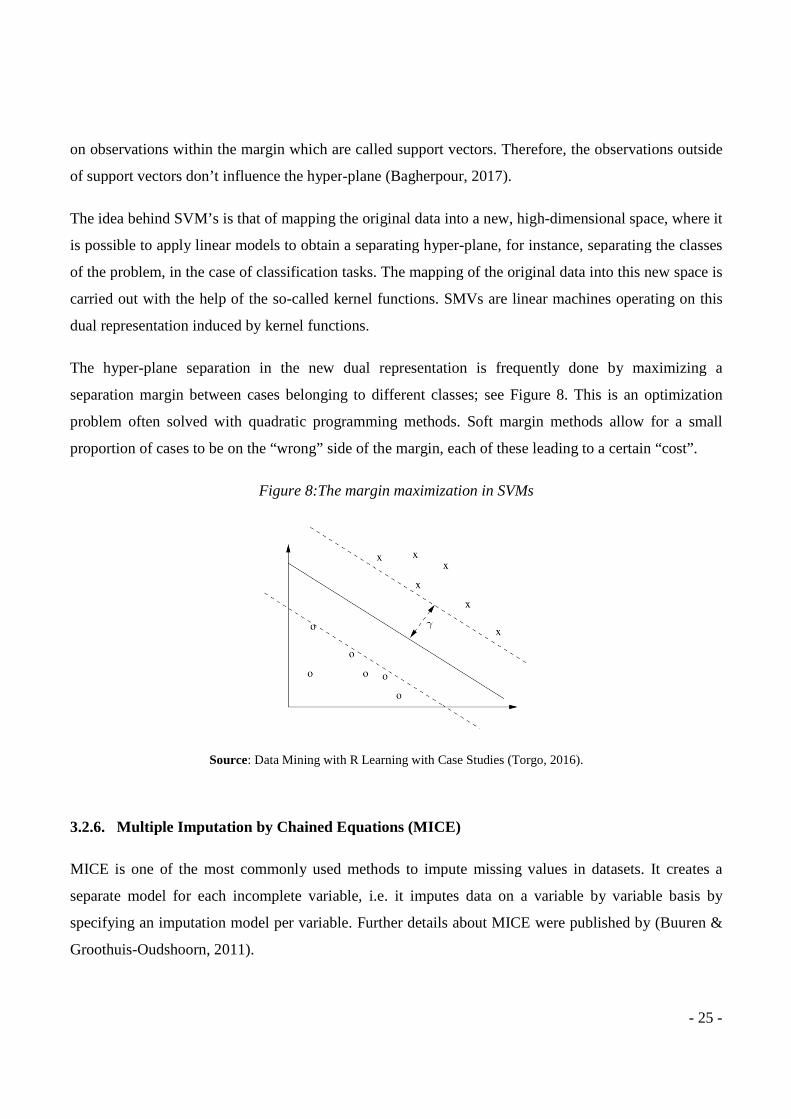
The hyper-plane separation in the new dual representation is frequently done by maximizing a

separation margin between cases belonging to different classes; see Figure

problem often solved with quadratic programming methods. Soft margin methods allow for a small

proportion of cases to be on the “wrong” side of the margin, each of these leading to a certain “cost”.

Figure

Source: Data

3.2.6. Multiple Imputation by Chained Equations (

MICE is one of the most commonly used methods to impute missing values in datasets. It creates a

separate model for each incomplete variable, i.e. it imputes data on a variable

specifying an imputation model per variable. Further details about MICE were published by

Groothuis-Oudshoorn, 2011).

on observations within the margin which are called support vectors. Therefore, the observations out

of support vectors don’t influence the hyper-plane (Bagherpour, 2017).

s is that of mapping the original data into a new, high-dimensional space, where it

is possible to apply linear models to obtain a separating hyper-plane, for instance, separating the classes


carried out with the help of the so-called kernel functions. SMVs are linear machines operating on this

entation induced by kernel functions.

plane separation in the new dual representation is frequently done by maximizing a

separation margin between cases belonging to different classes; see Figure 8

th quadratic programming methods. Soft margin methods allow for a small


Figure 8:The margin maximization in SVMs

: Data Mining with R Learning with Case Studies (Torgo, 2016)

Multiple Imputation by Chained Equations (MICE)


separate model for each incomplete variable, i.e. it imputes data on a variable

specifying an imputation model per variable. Further details about MICE were published by

- 25 -

on observations within the margin which are called support vectors. Therefore, the observations outside

dimensional space, where it

nstance, separating the classes


called kernel functions. SMVs are linear machines operating on this

plane separation in the new dual representation is frequently done by maximizing a

8. This is an optimization

th quadratic programming methods. Soft margin methods allow for a small


(Torgo, 2016).


separate model for each incomplete variable, i.e. it imputes data on a variable by variable basis by

specifying an imputation model per variable. Further details about MICE were published by (Buuren &

- 26 -

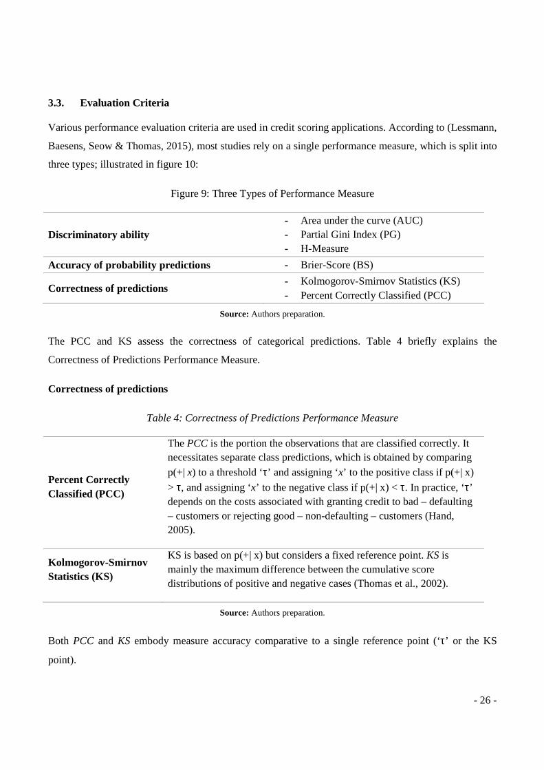
3.3. Evaluation Criteria

Various performance evaluation criteria are used in credit scoring applications. According to (Lessmann,

Baesens, Seow & Thomas, 2015), most studies rely on a single performance measure, which is split into

three types; illustrated in figure 10:

Figure 9: Three Types of Performance Measure

Discriminatory ability - Area under the curve (AUC) - Partial Gini Index (PG) - H-Measure

Accuracy of probability predictions - Brier-Score (BS)

Correctness of predictions - Kolmogorov-Smirnov Statistics (KS) - Percent Correctly Classified (PCC)


The PCC and KS assess the correctness of categorical predictions. Table 4 briefly explains the

Correctness of Predictions Performance Measure.

Correctness of predictions

Table 4: Correctness of Predictions Performance Measure

Percent Correctly Classified (PCC)

The PCC is the portion the observations that are classified correctly. It necessitates separate class predictions, which is obtained by comparing

p(+| x) to a threshold ‘τ’ and assigning ‘x’ to the positive class if p(+| x)

> τ, and assigning ‘x’ to the negative class if p(+| x) < τ. In practice, ‘τ’ depends on the costs associated with granting credit to bad – defaulting – customers or rejecting good – non-defaulting – customers (Hand, 2005).

Kolmogorov-Smirnov Statistics (KS)

KS is based on p(+| x) but considers a fixed reference point. KS is mainly the maximum difference between the cumulative score distributions of positive and negative cases (Thomas et al., 2002).


Both PCC and KS embody measure accuracy comparative to a single reference point (‘τ’ or the KS

point).

- 27 -

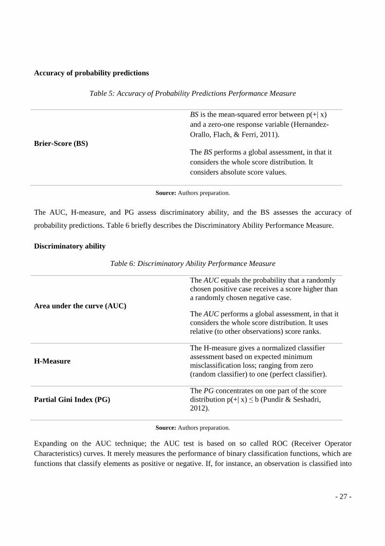
Accuracy of probability predictions

Table 5: Accuracy of Probability Predictions Performance Measure

Brier-Score (BS)

BS is the mean-squared error between p(+| x) and a zero-one response variable (Hernandez-Orallo, Flach, & Ferri, 2011).

The BS performs a global assessment, in that it considers the whole score distribution. It considers absolute score values.


The AUC, H-measure, and PG assess discriminatory ability, and the BS assesses the accuracy of

probability predictions. Table 6 briefly describes the Discriminatory Ability Performance Measure.

Discriminatory ability

Table 6: Discriminatory Ability Performance Measure

Area under the curve (AUC)

The AUC equals the probability that a randomly chosen positive case receives a score higher than a randomly chosen negative case.

The AUC performs a global assessment, in that it considers the whole score distribution. It uses relative (to other observations) score ranks.

H-Measure

The H-measure gives a normalized classifier assessment based on expected minimum misclassification loss; ranging from zero (random classifier) to one (perfect classifier).

Partial Gini Index (PG) The PG concentrates on one part of the score distribution p(+| x) ≤ b (Pundir & Seshadri, 2012).


Expanding on the AUC technique; the AUC test is based on so called ROC (Receiver Operator Characteristics) curves. It merely measures the performance of binary classification functions, which are functions that classify elements as positive or negative. If, for instance, an observation is classified into

- 28 -

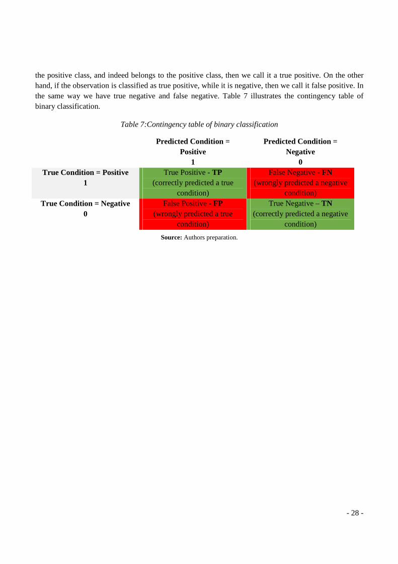
the positive class, and indeed belongs to the positive class, then we call it a true positive. On the other hand, if the observation is classified as true positive, while it is negative, then we call it false positive. In the same way we have true negative and false negative. Table 7 illustrates the contingency table of binary classification.

Table 7:Contingency table of binary classification

Predicted Condition = Positive

1

Predicted Condition = Negative

0 True Condition = Positive

1 True Positive - TP

(correctly predicted a true condition)

False Negative - FN (wrongly predicted a negative

condition) True Condition = Negative

0 False Positive - FP

(wrongly predicted a true condition)

True Negative – TN (correctly predicted a negative

condition)


Plotting the ROC Curve

ROC space is defined by FPR and TPR as

between true positive (benefits) and false positive (costs). The best possible prediction method would

yield a point in the upper left corner or coordinate (0,1) of the ROC space

(no false negatives) and 100% specificity (no false positives). The (0,1) point is also called a perfect

classification. A completely random guess would give a point along a diagonal line (the so

no-discrimination) from the left bottom to the top right corners (regardless of the positive and negative

base rates). An intuitive example of random guessing is a decision by flipping coins (heads or tails). As

the size of the sample increases, a random classifier's R

The diagonal divides the ROC space. Points above the diagonal represent good classification results

(better than random), points below the line represent poor results (worse than random).

Given that there is imbalance shown in

to reason whether and how class skew affects the performance measures. The

are not affected by class imbalance

imbalance as they are based on the score distribution of a classifier

class skew (Gong & Huang, 2012)

of AUC by plotting the ROC Curve

model’s accuracy.

R and TPR as ‘x’ and ‘y’ axes respectively, which depicts relative trade


yield a point in the upper left corner or coordinate (0,1) of the ROC space, representing 100% sensitivity


classification. A completely random guess would give a point along a diagonal line (the so

tion) from the left bottom to the top right corners (regardless of the positive and negative


the size of the sample increases, a random classifier's ROC point migrates towards (0.5,0.5).



Graph 1: ROC Space

Source: OpenEye Scientific.

there is imbalance shown in the class distributions in our data (see section 4.

to reason whether and how class skew affects the performance measures. The

t affected by class imbalance (Fawcett, 2005), however, the BS and the

based on the score distribution of a classifier, i.e. BS

(Gong & Huang, 2012). For this reason, in our project we consider

of AUC by plotting the ROC Curve a viable approach for classifier comparisons

- 29 -

axes respectively, which depicts relative trade-offs


, representing 100% sensitivity


classification. A completely random guess would give a point along a diagonal line (the so-called line of

tion) from the left bottom to the top right corners (regardless of the positive and negative


OC point migrates towards (0.5,0.5).



the class distributions in our data (see section 4.4), it is important

to reason whether and how class skew affects the performance measures. The AUC, PG, and H-measure

and the KS are affected by class

and KS are robust toward

we consider the performance measure

or classifier comparisons, highlighting the

- 30 -

4. Dataset Properties

In this section we present the data set used in our paper, which is publicly provided by Freddie Mac. The

dataset covers approximately 25.7 million fixed-rate mortgages originated between January 1, 1999 and

March 31, 2017. Monthly loan performance data, including credit performance information up to and

including property disposition, is being disclosed through September 30, 2017 (Freddie Mac Overview,

2018). Working on “Big” data, such as the one provided here, is quite a challenge given that it does not

only require a high-pitched computational power, but also most of the regular programs don’t have the

necessary capability to process such information. An unpretentious definition of Big Data is data that is

big in Volume, i.e. Tall and Wide Data. Various tools were introduced such as H20 Library, which uses

in-memory compression to handle billions of data even with a small cluster (Bash, 2015). Although this

state-of-art library is very promising dealing with our dataset, yet R-Studio still needs to load the dataset

onto the computer memory, which would not be currently sufficient. That said, we instead proceeded

with using Freddie Mac’s sample data, also available publicly on their website, which consists on

random samples of 50,000 loans selected from each full year. On these samples the website guarantees

the proportional number of loans from each partial year of the full Single-Family Loan-Level Dataset.

The Dataset includes two sets of files, Loan-level origination files, and monthly loan performance on a

portion of the fully amortizing 30-year fixed-rate Single Family mortgages that Freddie Mac acquired

with origination dates from 1999 to the Origination Cut-off Date. The Loan-Level origination file

contain information for each loan at the time of origination and Monthly Loan Performance Files

contain corresponding monthly performance data. That said, we have an eye on the loans that were

approved only, and not the ones that clients applied for, but their loans never went through.

4.1. Data Dictionary

In this section, we provide information regarding the layout of each file, origination and monthly

performance, that are available publicly on the website of Freddie Mac, in addition to information about

each data elements contained within each file type.

- 31 -

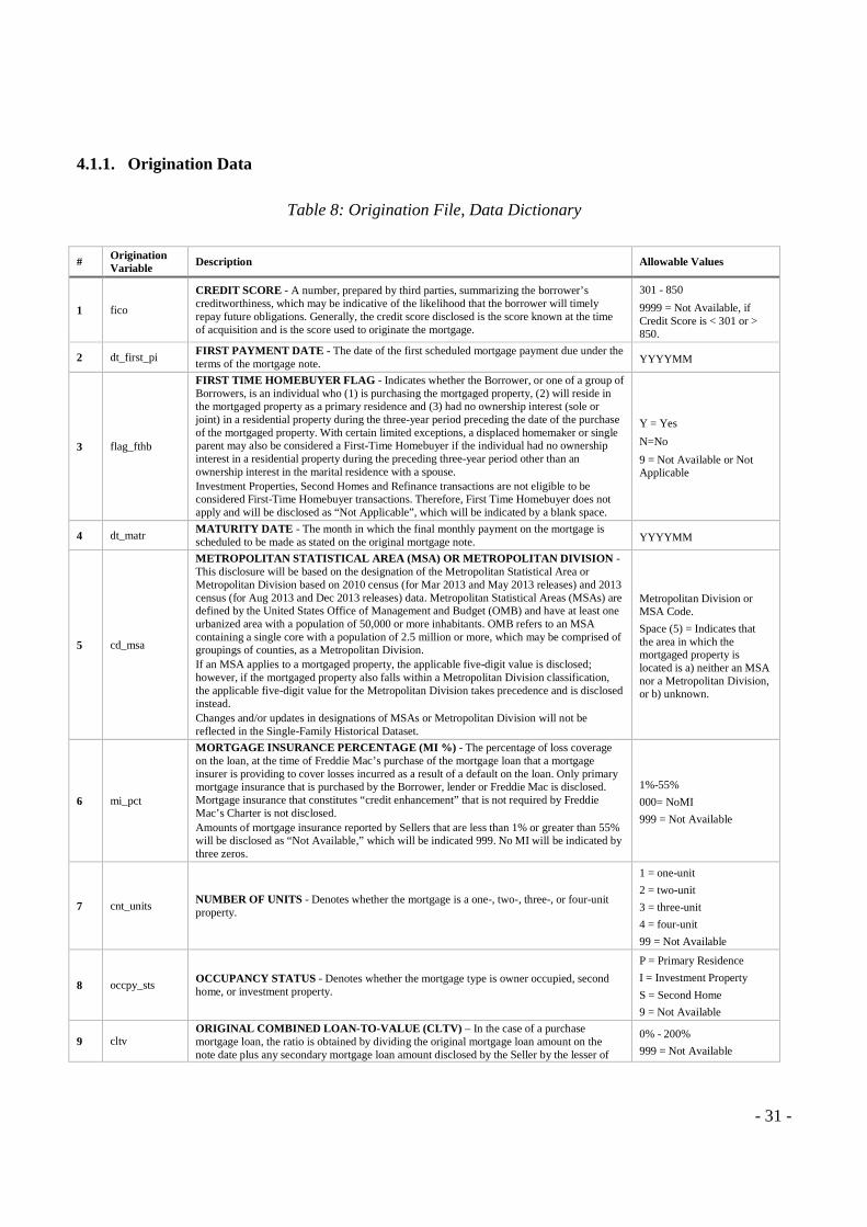
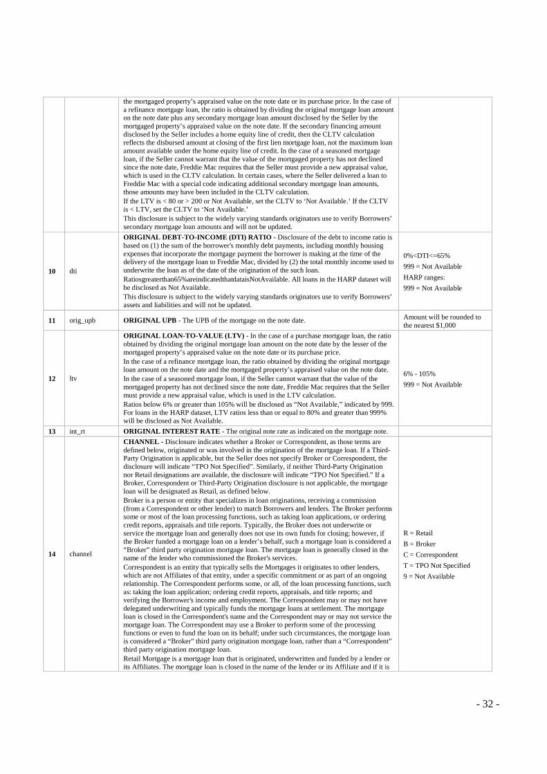
4.1.1. Origination Data

Table 8: Origination File, Data Dictionary

# Origination Variable Description Allowable Values

1 fico

CREDIT SCORE - A number, prepared by third parties, summarizing the borrower’s creditworthiness, which may be indicative of the likelihood that the borrower will timely repay future obligations. Generally, the credit score disclosed is the score known at the time of acquisition and is the score used to originate the mortgage.

301 - 850

9999 = Not Available, if Credit Score is < 301 or > 850.

2 dt_first_pi FIRST PAYMENT DATE - The date of the first scheduled mortgage payment due under the terms of the mortgage note. YYYYMM

3 flag_fthb

FIRST TIME HOMEBUYER FLAG - Indicates whether the Borrower, or one of a group of Borrowers, is an individual who (1) is purchasing the mortgaged property, (2) will reside in the mortgaged property as a primary residence and (3) had no ownership interest (sole or joint) in a residential property during the three-year period preceding the date of the purchase of the mortgaged property. With certain limited exceptions, a displaced homemaker or single parent may also be considered a First-Time Homebuyer if the individual had no ownership interest in a residential property during the preceding three-year period other than an ownership interest in the marital residence with a spouse. Investment Properties, Second Homes and Refinance transactions are not eligible to be considered First-Time Homebuyer transactions. Therefore, First Time Homebuyer does not apply and will be disclosed as “Not Applicable”, which will be indicated by a blank space.

Y = Yes

N=No

9 = Not Available or Not Applicable

4 dt_matr MATURITY DATE - The month in which the final monthly payment on the mortgage is scheduled to be made as stated on the original mortgage note. YYYYMM

5 cd_msa

METROPOLITAN STATISTICAL AREA (MSA) OR METROPOLITAN DIVISION - This disclosure will be based on the designation of the Metropolitan Statistical Area or Metropolitan Division based on 2010 census (for Mar 2013 and May 2013 releases) and 2013 census (for Aug 2013 and Dec 2013 releases) data. Metropolitan Statistical Areas (MSAs) are defined by the United States Office of Management and Budget (OMB) and have at least one urbanized area with a population of 50,000 or more inhabitants. OMB refers to an MSA containing a single core with a population of 2.5 million or more, which may be comprised of groupings of counties, as a Metropolitan Division. If an MSA applies to a mortgaged property, the applicable five-digit value is disclosed; however, if the mortgaged property also falls within a Metropolitan Division classification, the applicable five-digit value for the Metropolitan Division takes precedence and is disclosed instead. Changes and/or updates in designations of MSAs or Metropolitan Division will not be reflected in the Single-Family Historical Dataset.

Metropolitan Division or MSA Code.

Space (5) = Indicates that the area in which the mortgaged property is located is a) neither an MSA nor a Metropolitan Division, or b) unknown.

6 mi_pct

MORTGAGE INSURANCE PERCENTAGE (MI %) - The percentage of loss coverage on the loan, at the time of Freddie Mac’s purchase of the mortgage loan that a mortgage insurer is providing to cover losses incurred as a result of a default on the loan. Only primary mortgage insurance that is purchased by the Borrower, lender or Freddie Mac is disclosed. Mortgage insurance that constitutes “credit enhancement” that is not required by Freddie Mac’s Charter is not disclosed. Amounts of mortgage insurance reported by Sellers that are less than 1% or greater than 55% will be disclosed as “Not Available,” which will be indicated 999. No MI will be indicated by three zeros.

1%-55%

000= NoMI

999 = Not Available

7 cnt_units NUMBER OF UNITS - Denotes whether the mortgage is a one-, two-, three-, or four-unit property.

1 = one-unit

2 = two-unit

3 = three-unit

4 = four-unit

99 = Not Available

8 occpy_sts OCCUPANCY STATUS - Denotes whether the mortgage type is owner occupied, second home, or investment property.

P = Primary Residence

I = Investment Property

S = Second Home

9 = Not Available

9 cltv ORIGINAL COMBINED LOAN-TO-VALUE (CLTV) – In the case of a purchase mortgage loan, the ratio is obtained by dividing the original mortgage loan amount on the note date plus any secondary mortgage loan amount disclosed by the Seller by the lesser of

0% - 200%

999 = Not Available

- 32 -

the mortgaged property’s appraised value on the note date or its purchase price. In the case of a refinance mortgage loan, the ratio is obtained by dividing the original mortgage loan amount on the note date plus any secondary mortgage loan amount disclosed by the Seller by the mortgaged property’s appraised value on the note date. If the secondary financing amount disclosed by the Seller includes a home equity line of credit, then the CLTV calculation reflects the disbursed amount at closing of the first lien mortgage loan, not the maximum loan amount available under the home equity line of credit. In the case of a seasoned mortgage loan, if the Seller cannot warrant that the value of the mortgaged property has not declined since the note date, Freddie Mac requires that the Seller must provide a new appraisal value, which is used in the CLTV calculation. In certain cases, where the Seller delivered a loan to Freddie Mac with a special code indicating additional secondary mortgage loan amounts, those amounts may have been included in the CLTV calculation. If the LTV is < 80 or > 200 or Not Available, set the CLTV to ‘Not Available.’ If the CLTV is < LTV, set the CLTV to ‘Not Available.’ This disclosure is subject to the widely varying standards originators use to verify Borrowers’ secondary mortgage loan amounts and will not be updated.

10 dti

ORIGINAL DEBT-TO-INCOME (DTI) RATIO - Disclosure of the debt to income ratio is based on (1) the sum of the borrower's monthly debt payments, including monthly housing expenses that incorporate the mortgage payment the borrower is making at the time of the delivery of the mortgage loan to Freddie Mac, divided by (2) the total monthly income used to underwrite the loan as of the date of the origination of the such loan. Ratiosgreaterthan65%areindicatedthatdataisNotAvailable. All loans in the HARP dataset will be disclosed as Not Available. This disclosure is subject to the widely varying standards originators use to verify Borrowers’ assets and liabilities and will not be updated.

0%<DTI<=65%

999 = Not Available

HARP ranges:

999 = Not Available

11 orig_upb ORIGINAL UPB - The UPB of the mortgage on the note date. Amount will be rounded to the nearest $1,000

12 ltv

ORIGINAL LOAN-TO-VALUE (LTV) - In the case of a purchase mortgage loan, the ratio obtained by dividing the original mortgage loan amount on the note date by the lesser of the mortgaged property’s appraised value on the note date or its purchase price. In the case of a refinance mortgage loan, the ratio obtained by dividing the original mortgage loan amount on the note date and the mortgaged property’s appraised value on the note date. In the case of a seasoned mortgage loan, if the Seller cannot warrant that the value of the mortgaged property has not declined since the note date, Freddie Mac requires that the Seller must provide a new appraisal value, which is used in the LTV calculation. Ratios below 6% or greater than 105% will be disclosed as “Not Available,” indicated by 999. For loans in the HARP dataset, LTV ratios less than or equal to 80% and greater than 999% will be disclosed as Not Available.

6% - 105%

999 = Not Available

13 int_rt ORIGINAL INTEREST RATE - The original note rate as indicated on the mortgage note.

14 channel

CHANNEL - Disclosure indicates whether a Broker or Correspondent, as those terms are defined below, originated or was involved in the origination of the mortgage loan. If a Third-Party Origination is applicable, but the Seller does not specify Broker or Correspondent, the disclosure will indicate “TPO Not Specified”. Similarly, if neither Third-Party Origination nor Retail designations are available, the disclosure will indicate “TPO Not Specified.” If a Broker, Correspondent or Third-Party Origination disclosure is not applicable, the mortgage loan will be designated as Retail, as defined below. Broker is a person or entity that specializes in loan originations, receiving a commission (from a Correspondent or other lender) to match Borrowers and lenders. The Broker performs some or most of the loan processing functions, such as taking loan applications, or ordering credit reports, appraisals and title reports. Typically, the Broker does not underwrite or service the mortgage loan and generally does not use its own funds for closing; however, if the Broker funded a mortgage loan on a lender’s behalf, such a mortgage loan is considered a “Broker” third party origination mortgage loan. The mortgage loan is generally closed in the name of the lender who commissioned the Broker's services. Correspondent is an entity that typically sells the Mortgages it originates to other lenders, which are not Affiliates of that entity, under a specific commitment or as part of an ongoing relationship. The Correspondent performs some, or all, of the loan processing functions, such as: taking the loan application; ordering credit reports, appraisals, and title reports; and verifying the Borrower's income and employment. The Correspondent may or may not have delegated underwriting and typically funds the mortgage loans at settlement. The mortgage loan is closed in the Correspondent's name and the Correspondent may or may not service the mortgage loan. The Correspondent may use a Broker to perform some of the processing functions or even to fund the loan on its behalf; under such circumstances, the mortgage loan is considered a “Broker” third party origination mortgage loan, rather than a “Correspondent” third party origination mortgage loan. Retail Mortgage is a mortgage loan that is originated, underwritten and funded by a lender or its Affiliates. The mortgage loan is closed in the name of the lender or its Affiliate and if it is

R = Retail

B = Broker

C = Correspondent

T = TPO Not Specified

9 = Not Available

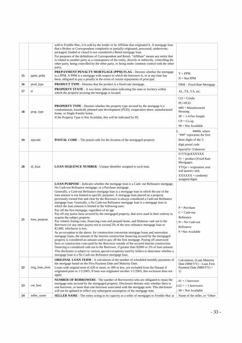
- 33 -

sold to Freddie Mac, it is sold by the lender or its Affiliate that originated it. A mortgage loan that a Broker or Correspondent completely or partially originated, processed, underwrote, packaged, funded or closed is not considered a Retail mortgage loan. For purposes of the definitions of Correspondent and Retail, “Affiliate" means any entity that is related to another party as a consequence of the entity, directly or indirectly, controlling the other party, being controlled by the other party, or being under common control with the other party.

15 ppmt_pnlty PREPAYMENT PENALTY MORTGAGE (PPM) FLAG - Denotes whether the mortgage is a PPM. A PPM is a mortgage with respect to which the borrower is, or at any time has been, obligated to pay a penalty in the event of certain repayments of principal.

Y = PPM

N = Not PPM

16 prod_type PRODUCT TYPE - Denotes that the product is a fixed-rate mortgage. FRM – Fixed Rate Mortgage

17 st PROPERTY STATE - A two-letter abbreviation indicating the state or territory within which the property securing the mortgage is located. AL, TX, VA, etc.

18 prop_type

PROPERTY TYPE - Denotes whether the property type secured by the mortgage is a condominium, leasehold, planned unit development (PUD), cooperative share, manufactured home, or Single-Family home. If the Property Type is Not Available, this will be indicated by 99.

CO = Condo

PU=PUD

MH = Manufactured Housing

SF = 1-4 Fee Simple

CP = Co-op

99 = Not Available

19 zipcode POSTAL CODE – The postal code for the location of the mortgaged property

mm. ###00, where “###” represents the first

three digits of the 5-

digit postal code

Space(5)= Unknown

20 id_loan LOAN SEQUENCE NUMBER - Unique identifier assigned to each loan.

F1YYQnXXXXXX

F1 = product (Fixed Rate Mortgage);

YYQn = origination year and quarter; and,

XXXXXX = randomly assigned digits

21 loan_purpose

LOAN PURPOSE - Indicates whether the mortgage loan is a Cash- out Refinance mortgage, No Cash-out Refinance mortgage, or a Purchase mortgage. Generally, a Cash-out Refinance mortgage loan is a mortgage loan in which the use of the loan amount is not limited to specific purposes. A mortgage loan placed on a property previously owned free and clear by the Borrower is always considered a Cash-out Refinance mortgage loan. Generally, a No Cash-out Refinance mortgage loan is a mortgage loan in which the loan amount is limited to the following uses: Pay off the first mortgage, regardless of its age Pay off any junior liens secured by the mortgaged property, that were used in their entirety to acquire the subject property Pay related closing costs, financing costs and prepaid items, and Disburse cash out to the Borrower (or any other payee) not to exceed 2% of the new refinance mortgage loan or $2,000, whichever is less. As an exception to the above, for construction conversion mortgage loans and renovation mortgage loans, the amount of the interim construction financing secured by the mortgaged property is considered an amount used to pay off the first mortgage. Paying off unsecured liens or construction costs paid by the Borrower outside of the secured interim construction financing is considered cash out to the Borrower, if greater than $2000 or 2% of loan amount. This disclosure is subject to various special exceptions used by Sellers to determine whether a mortgage loan is a No Cash-out Refinance mortgage loan.

P = Purchase

C = Cash-out

Refinance

ww. N = No Cash-out

Refinance

9 =Not Available

22 orig_loan_term

ORIGINAL LOAN TERM - A calculation of the number of scheduled monthly payments of the mortgage based on the First Payment Date and Maturity Date. Loans with original term of 420 or more, or 300 or less, are excluded from the Dataset if originated prior to 1/1/2005. If loan was originated on/after 1/1/2005, this exclusion does not apply.

Calculation: (Loan Maturity Date (MM/YY) – Loan First Payment Date (MM/YY) + 1)

23 cnt_borr

NUMBER OF BORROWERS - The number of Borrower(s) who are obligated to repay the mortgage note secured by the mortgaged property. Disclosure denotes only whether there is one borrower, or more than one borrower associated with the mortgage note. This disclosure will not be updated to reflect any subsequent assumption of the mortgage note.

aaa. 01 = 1 borrower

bbb. 02 = > 1 borrowers

ccc. 99 = Not Available

24 seller_name SELLER NAME - The entity acting in its capacity as a seller of mortgages to Freddie Mac at Name of the seller, or “Other

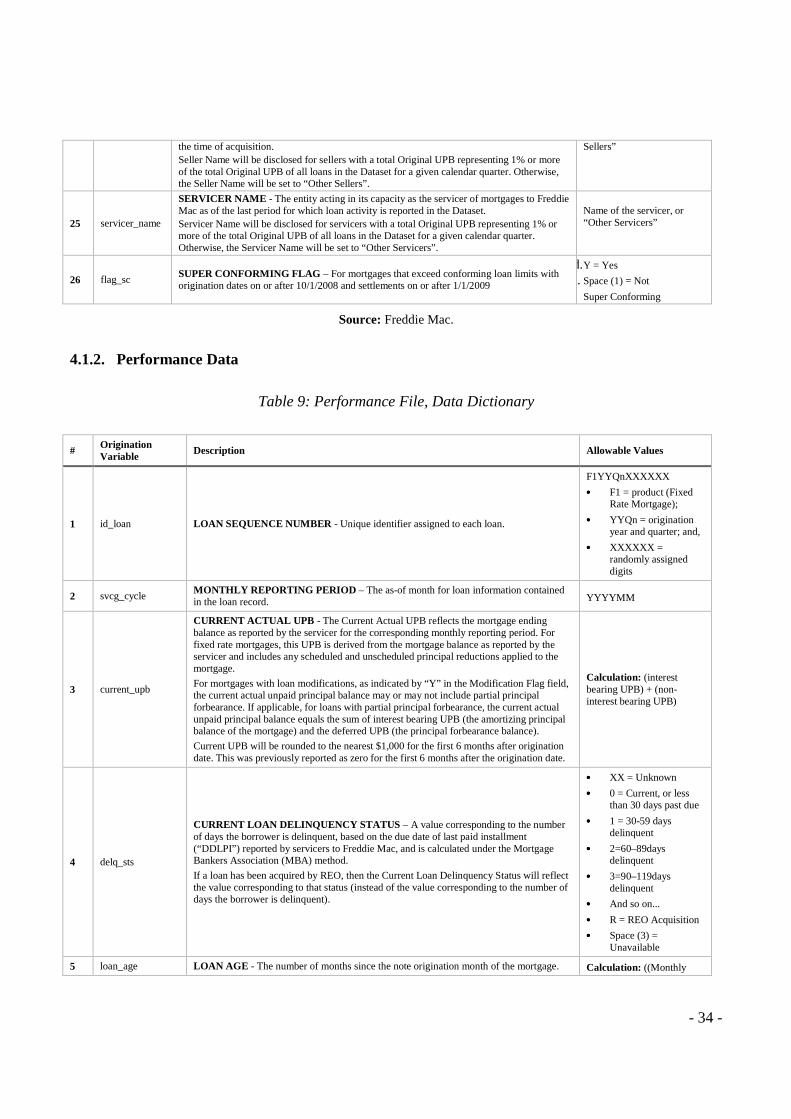
- 34 -

the time of acquisition. Seller Name will be disclosed for sellers with a total Original UPB representing 1% or more of the total Original UPB of all loans in the Dataset for a given calendar quarter. Otherwise, the Seller Name will be set to “Other Sellers”.

Sellers”

25 servicer_name

SERVICER NAME - The entity acting in its capacity as the servicer of mortgages to Freddie Mac as of the last period for which loan activity is reported in the Dataset. Servicer Name will be disclosed for servicers with a total Original UPB representing 1% or more of the total Original UPB of all loans in the Dataset for a given calendar quarter. Otherwise, the Servicer Name will be set to “Other Servicers”.

Name of the servicer, or “Other Servicers”

26 flag_sc SUPER CONFORMING FLAG – For mortgages that exceed conforming loan limits with origination dates on or after 10/1/2008 and settlements on or after 1/1/2009

ddd. Y = Yes

eee. Space (1) = Not

Super Conforming

Source: Freddie Mac.

4.1.2. Performance Data

Table 9: Performance File, Data Dictionary

# Origination Variable

Description Allowable Values

1 id_loan LOAN SEQUENCE NUMBER - Unique identifier assigned to each loan.

F1YYQnXXXXXX

•••• F1 = product (Fixed Rate Mortgage);

•••• YYQn = origination year and quarter; and,

•••• XXXXXX = randomly assigned digits

2 svcg_cycle MONTHLY REPORTING PERIOD – The as-of month for loan information contained in the loan record. YYYYMM

3 current_upb

CURRENT ACTUAL UPB - The Current Actual UPB reflects the mortgage ending balance as reported by the servicer for the corresponding monthly reporting period. For fixed rate mortgages, this UPB is derived from the mortgage balance as reported by the servicer and includes any scheduled and unscheduled principal reductions applied to the mortgage.

For mortgages with loan modifications, as indicated by “Y” in the Modification Flag field, the current actual unpaid principal balance may or may not include partial principal forbearance. If applicable, for loans with partial principal forbearance, the current actual unpaid principal balance equals the sum of interest bearing UPB (the amortizing principal balance of the mortgage) and the deferred UPB (the principal forbearance balance).

Current UPB will be rounded to the nearest $1,000 for the first 6 months after origination date. This was previously reported as zero for the first 6 months after the origination date.

Calculation: (interest bearing UPB) + (non- interest bearing UPB)

4 delq_sts

CURRENT LOAN DELINQUENCY STATUS – A value corresponding to the number of days the borrower is delinquent, based on the due date of last paid installment (“DDLPI”) reported by servicers to Freddie Mac, and is calculated under the Mortgage Bankers Association (MBA) method.

If a loan has been acquired by REO, then the Current Loan Delinquency Status will reflect the value corresponding to that status (instead of the value corresponding to the number of days the borrower is delinquent).

•••• XX = Unknown

•••• 0 = Current, or less than 30 days past due

•••• 1 = 30-59 days delinquent

•••• 2=60–89days delinquent

•••• 3=90–119days delinquent

•••• And so on...

•••• R = REO Acquisition

•••• Space (3) = Unavailable

5 loan_age LOAN AGE - The number of months since the note origination month of the mortgage. Calculation: ((Monthly

- 35 -

To ensure the age measurement commences with the first full month after the note origination month, subtract 1.

Reporting Period) – Loan Origination Date (MM/YY)) – 1 month

6 mths_remng

REMAINING MONTHS TO LEGAL MATURITY - The remaining number of months to the mortgage maturity date.

For mortgages with loan modifications, as indicated by “Y” in the Modification Flag field, the calculation uses the modified maturity date.

Calculation: (Maturity Date (MM/YY) – Monthly Reporting Period (MM/YY)

7 repch_flag REPURCHASE FLAG - Indicates loans that have been repurchased or made whole (not inclusive of pool-level repurchase settlements).

This field is only populated only at loan termination month.

•••• N = Not Repurchased

•••• Y = Repurchased

•••• Space (1) = Not Applicable

8 flag_mod MODIFICATION FLAG – For mortgages with loan modifications, indicates that the loan has been modified.

•••• Y = Yes

•••• Space (1) = Not Modified

9 cd_zero_bal ZERO BALANCE CODE - A code indicating the reason the loan's balance was reduced to zero.

•••• 01 = Prepaid or Matured (Voluntary Payoff)

•••• 02 = Third Party Sale

•••• 03=ShortSale or Charge Off

•••• 06 = Repurchase prior to Property Disposition

•••• 09 = REO Disposition

•••• 15 = Note sale/Reperforming sale

10 dt_zero_bal ZERO BALANCE EFFECTIVE DATE - The date on which the event triggering the Zero Balance Code took place.

•••• YYYYMM

•••• Space(6) = Not Applicable

11 current_int_rt CURRENT INTEREST RATE - Reflects the current interest rate on the mortgage note, considering any loan modifications.

12 non_int_brng_upb CURRENT DEFERRED UPB: The current non-interest bearing UPB of the modified mortgage.

$ Amount. Non-Interest Bearing UPB.

13 dt_lst_pi DUE DATE OF LAST PAID INSTALLMENT (DDLPI) : The due date that the loan’s scheduled principal and interest is paid through, regardless of when the installment payment was actually made.

•••• YYYYMM

14 mi_recoveries MI RECOVERIES - Mortgage Insurance Recoveries are proceeds received by Freddie Mac in the event of credit losses. These proceeds are based on claims under a mortgage insurance policy.

$ Amount. MI Recoveries.

15 net_sale_proceeds

NET SALES PROCEEDS - The amount remitted to Freddie Mac resulting from a property disposition or loan sale (which in the case of bulk sales, may be an allocated amount) once allowable selling expenses have been deducted from the gross sales proceeds.

A value of “C” in Net Sales Proceeds stands for Covered, which means that as part of the property disposition process, Freddie Mac was “Covered” for its total indebtedness (defined as UPB at disposition plus delinquent accrued interest) and net sale proceeds covered default expenses incurred by Servicer during the disposal of the loan.

A value of “U” indicates that the amount is unknown.

$ Amount. Gross Sale Proceeds – Allowable Selling Expenses.

C = Covered U = Unknown

16 non_mi_recoveries

NON-MI RECOVERIES : Non-MI Recoveries are proceeds received by Freddie Mac based on repurchase/make whole proceeds, non-sale income such as refunds (tax or insurance), hazard insurance proceeds, rental receipts, positive escrow and/or other miscellaneous credits.

$ Amount. Non-MI Recoveries.

17 expenses

EXPENSES - Expenses will include allowable expenses that Freddie Mac bears in the process of acquiring, maintaining and/ or disposing a property (excluding selling expenses, which are subtracted from gross sales proceeds to derive net sales proceeds). This is an aggregation of Legal Costs, Maintenance and Preservation Costs, Taxes and Insurance, and Miscellaneous Expenses

$ Amount. Allowable Expenses.

- 36 -

18 legal_costs

LEGAL COSTS - The amount of legal costs associated with the sale of a property (but not included in Net Sale Proceeds). Prior to population of a Zero Balance Code equal to 03 or 09, this field will be populated as “Not Applicable,” Following population of a Zero Balance Code equal to 03 or 09, this field will be updated (as applicable) to reflect the cumulative total. Space(12) – Not applicable

$ Amount

19 maint_pres_costs

MAINTENANCE AND PRESERVATION COSTS – The amount of maintenance, preservation, and repair costs, including but not limited to property inspection, homeowner’s association, utilities, and REO management, that is associated with the sale of a property (but not included in Net Sale Proceeds). Prior to population of a Zero Balance Code equal to 03 or 09, this field will be populated as “Not Applicable,” Following population of a Zero Balance Code equal to 03 or 09, this field will be updated (as applicable) to reflect the cumulative total. Space (12) – Not applicable

$ Amount

20 taxes_ins_costs

TAXES AND INSURANCE – The amount of taxes and insurance owed that are associated with the sale of a property (but not included in Net Sale Proceeds). Prior to population of a Zero Balance Code equal to 03 or 09, this field will be populated as “Not Applicable,”. Following population of a Zero Balance Code equal to 03 or 09, this field will be updated (as applicable) to reflect the cumulative total. Space(12) – Not applicable

$ Amount

21 misc_costs

MISCELLANEOUS EXPENSES - Miscellaneous expenses associated with the sales of the property but not included in Net Sale Proceeds). Prior to population of a Zero Balance Code equal to 03 or 09, this field will be populated as “Not Applicable,”. Following population of a Zero Balance Code equal to 03 or 09, this field will be updated (as applicable) to reflect the cumulative total. Space(12) – Not applicable.

$ Amount

22 actual_loss

ACTUAL LOSS CALCULATION - Actual Loss was calculated using the below approach:

Actual Loss = (Default UPB – Net Sale_Proceeds) + Delinquent Accrued Interest - Expenses – MI Recoveries – Non-MI Recoveries.

Delinquent Accrued Interest = (Default_Upb – Non-Interest bearing UPB) * (Current Interest rate – 0.35) * (Months between Last Principal & Interest paid to date and zero balance date) * 30/360/100.

Please note that the following business rules are applied to this calculation:

i. For all loans, 35 bps is used as a proxy for servicing fee

ii. The Actual Loss Calculation will be set to zero for loans with Repurchase Flag =’Y

iii. The Actual Loss Calculation will be set to zero for loans with Net Sale Proceeds = C (Covered)

iv. The Actual Loss Calculation will be set to zero for loans with Net Sales Proceeds = ‘U” (Net Sales Proceeds are missing, or expenses are not available.

v. The Actual Loss Calculation will be set to missing for loans disposed within three months prior to the performance cutoff date.

vi. Modification Costs are currently not included in the calculation of the Actual Loss Calculation Field

$ Amount

23 modcost

MODIFICATION COST - The cumulative modification cost amount calculated when Freddie Mac determines such mortgage loan has experienced a rate modification event. Modification Cost

is applicable for loans with rate changes only. This amount will be calculated on a monthly basis beginning with the first reporting period a modification event is reported and disclosed in the last performance record.

For example:

(Original Interest Rate/1200 * Current Actual UPB) – (Current Interest Rate/1200 * (sum (Current Actual UPB, -Current Deferred UPB)) and aggregate each month since modification through the Performance Cutoff Date into a cumulative amount

$ Amount

24 stepmod_ind STEP MODIFICATION FLAG – A Y/N flag will be disclosed for every modified loan, to denote if the terms of modification agreement call for note rate to increase over time.

•••• Y = Yes

•••• N=No

•••• Space (1) = Not Step Mod

25 dpm_ind DEFERRED PAYMENT MODIFICATION – A Y/N flag will be disclosed to indicate Deferred Payment Modification for the loan.

•••• Y = Yes

•••• N=No

Source: Freddie Mac.

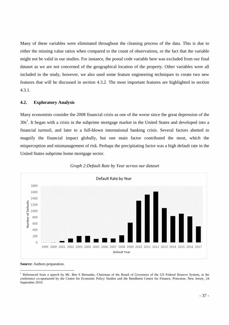
- 37 -

Many of these variables were eliminated throughout the cleaning process of the data. This is due to

either the missing value ratios when compared to the count of observations, or the fact that the variable

might not be valid in our studies. For instance, the postal code variable here was excluded from our final

dataset as we are not concerned of the geographical location of the property. Other variables were all

included in the study, however, we also used some feature engineering techniques to create two new

features that will be discussed in section 4.3.2. The most important features are highlighted in section

4.3.1.

4.2. Exploratory Analysis

Many economists consider the 2008 financial crisis as one of the worse since the great depression of the

30s1. It began with a crisis in the subprime mortgage market in the United States and developed into a

financial turmoil, and later to a full-blown international banking crisis. Several factors abetted to

magnify the financial impact globally, but one main factor contributed the most, which the

misperception and mismanagement of risk. Perhaps the precipitating factor was a high default rate in the

United States subprime home mortgage sector.

Graph 2:Default Rate by Year across our dataset


1 Referenced from a speech by Mr. Ben S Bernanke, Chairman of the Board of Governors of the US Federal Reserve System, at the conference co-sponsored by the Centre for Economic Policy Studies and the Bendheim Centre for Finance, Princeton, New Jersey, 24 September 2010.

0

200

400

600

800

1000

1200

1400

1600

1800

1999 2000 2001 2002 2003 2004 2005 2006 2007 2008 2009 2010 2011 2012 2013 2014 2015 2016 2017

Nu

mb

er o

f D

efa

ult

s

Default Year

Default Rate by Year

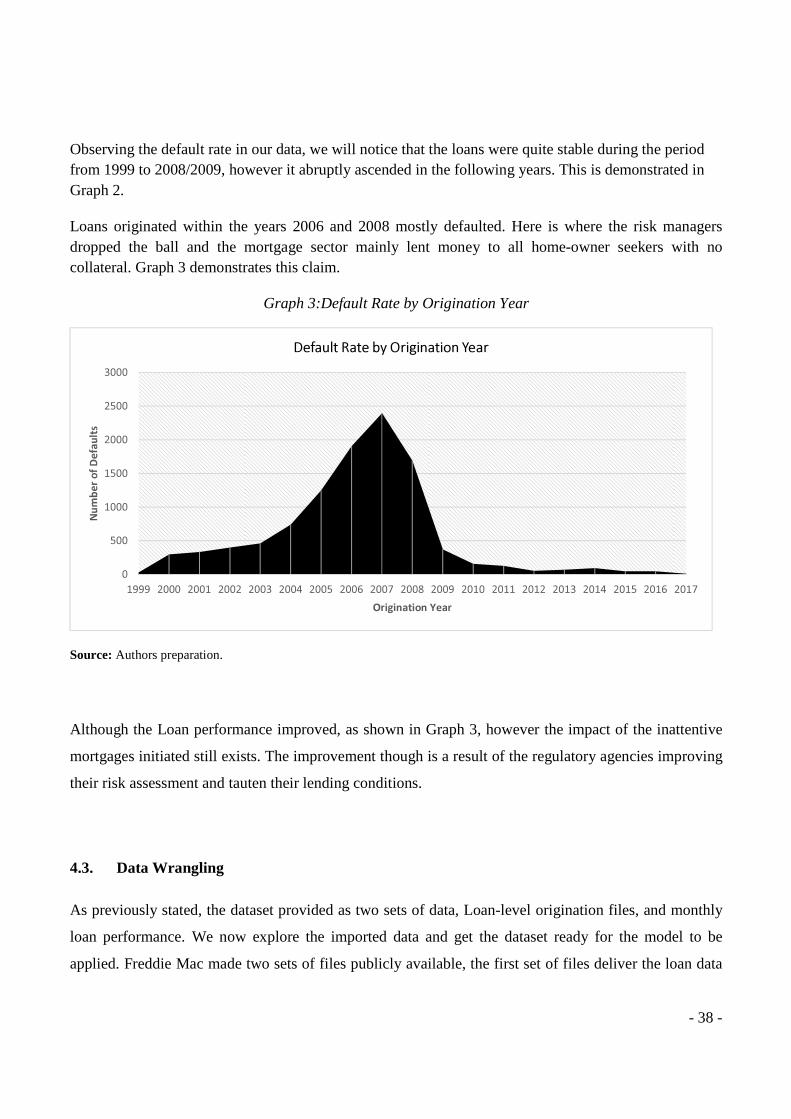
- 38 -

Observing the default rate in our data, we will notice that the loans were quite stable during the period from 1999 to 2008/2009, however it abruptly ascended in the following years. This is demonstrated in Graph 2.

Loans originated within the years 2006 and 2008 mostly defaulted. Here is where the risk managers dropped the ball and the mortgage sector mainly lent money to all home-owner seekers with no collateral. Graph 3 demonstrates this claim.

Graph 3:Default Rate by Origination Year


Although the Loan performance improved, as shown in Graph 3, however the impact of the inattentive

mortgages initiated still exists. The improvement though is a result of the regulatory agencies improving

their risk assessment and tauten their lending conditions.

4.3. Data Wrangling

As previously stated, the dataset provided as two sets of data, Loan-level origination files, and monthly

loan performance. We now explore the imported data and get the dataset ready for the model to be

applied. Freddie Mac made two sets of files publicly available, the first set of files deliver the loan data

0

500

1000

1500

2000

2500

3000

1999 2000 2001 2002 2003 2004 2005 2006 2007 2008 2009 2010 2011 2012 2013 2014 2015 2016 2017

Nu

mb

er o

f D

efa

ult

s

Origination Year

Default Rate by Origination Year

- 39 -

at the moment of origination, and the set of files deliver the loan performance on monthly basis. File

layouts and data dictionary were provided in section 4.1. and 4.2., representing loan-level origination

files and loan-level performance files respectively.

• Loan-level Origination Files

We created a data frame where we append all the data from the sample files for the years 1999 to

2017. The appended file has 26 variables which holds various details associated with the loan

origination annually. An important variable here is the Loan ID, which will be used later to link

the loan performance appended file to the origination one. The Loan ID is unique in the

origination file.

• Loan-level Performance Files

We created a data frame where we append all the data from the sample files for the years 1999 to

2017. The appended file has 23 variables which holds various details associated with the

borrower status quo on monthly basis. In this file, the Loan ID is not unique as it contains the

loan performance on monthly basis, so within one year the Loan ID might be repeated twelve

times (if the loan did not default). Therefore, our next step is to ensure the Loan ID variable is

distinguished. That said, we selected only the Loan ID with the highest Loan age value, as this

would represent the final outcome of the selected loan, whether it was defaulted or not.

4.3.1. Feature Importance

Subsequently, we join the two sets of data, Origination and Performance ones by our Unique variable,

the Loan ID, but before we proceed any further, it is imperative to select which attributes in our data that

are most relevant to the predictive model that we are building. (Guyon & Elisseeff, 2003) highlighted

that the objective of variable selection is threefold: improving the prediction performance of the

predictors, providing faster and more cost-effective predictors, and providing a better understanding of

the underlying process that generated the data.

- 40 -

Propitiously, Caret R Package can automatically rank all variables available by its importance by

building a model. This package can also remove any redundant variables by building a correlation

matrix of the data’s attributes and reports on attributes that are highly correlated with each other, which

can be removed. For simplicity, we will be ranking our variables by importance in our project. One of

the most widely used model that presents the importance of a variable in a dataset is Random Forest

(RF). Constructing this model, we discover that the “Zero Balance Code”, and the “Current Loan

Delinquency Status” are ranked the highest. Both variables play an instrumental role in determining

whether a loan defaulted or not. “Loan Age”, “Credit Score”, and “Original Combined Loan-to-Value”

were also in the list.

4.3.2. Feature Engineering

Before engineering a new feature (or variable), we studied the variables that would reflect to us which

loan has defaulted and which has not. Based on the definition provided by Freddie Mac, each loan

should be in one of three stages: Prepaid (loans that were fully paid before or after the expiration of the

mortgage), Paying (loans that are still active), and Default (loans that were not fully paid).

• Default Status Variable

We calculated default using current loan delinquency status given in the data. Delinquency status

measures the number of days the borrower is delinquent (i.e. couldn’t meet up with monthly

obligations) as specified by Freddie Mac. In the data, status 0 implies current or less than 30 days,

status 1 implies greater than 30 days but less than 60 days, status 2 implies greater than 60 days but

less than 90 days while status 3 refers to delinquency for days between 90 and 119. We calculated

maximum delinquency status for each loan and then specify the output variable as follows: if the

maximum delinquency status is greater than 3 (i.e. loan is of delinquency status 3 and above) or zero

balance code is greater than 9 (zero balance code is used to indicate why the loan balance was

reduced to zero, 09 indicates deed in lieu loans) we classify such loan as default. If the zero-balance

code is 01 (01 indicates prepaid or matured loans) we classify such loans as prepaid, the rest of the

loans we classify as paying. New feature (Default Status) is engineered to represent the final

outcome of each loan.

- 41 -

• Credit Scoring Variable

This newly created variable reflects another aspect of the borrower, which defines whether this

borrower is “good” or “bad”. This is merely based on the FICO score provided in the data set. Any

Borrower with 550 credit score or above is considered as a “good” borrower, lower than 550 is

considered as a “bad” borrower.

4.3.3. Missing Observations

To visually explore the missing values, we plot the number of missing values for each variable. Graph

04 represents the variables on the ‘y’ axis and the volume of the missing items on the ‘x’ axis. We have

almost 10 Variables with 100% of its observations are not available. Whether these variables were

missing at random or not, we will exclude them from our studies as it will not be possible to be imputed.

Graph 05 is the new representation of missing values versus variables after eliminating the variables

with no observations. All the remaining missing values were imputes using mice. Mice merely builds a

separate model for each missing observation and imputes it using all the observations in the given

variables.

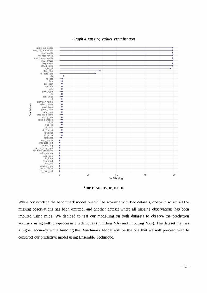
- 42 -

Graph 4:Missing Values Visualization


While constructing the benchmark model, we will be working with two datasets, one with which all the

missing observations has been omitted, and another dataset where all missing observations has been

imputed using mice. We decided to test our modelling on both datasets to observe the prediction

accuracy using both pre-processing techniques (Omitting NAs and Imputing NAs). The dataset that has

a higher accuracy while building the Benchmark Model will be the one that we will proceed with to

construct our predictive model using Ensemble Technique.

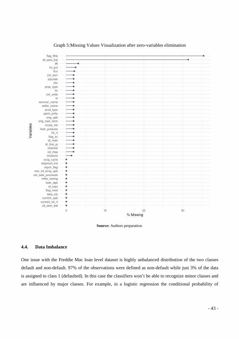
- 43 -

Graph 5:Missing Values Visualization after zero-variables elimination


4.4. Data Imbalance

One issue with the Freddie Mac loan level dataset is highly unbalanced distribution of the two classes

default and non-default. 97% of the observations were defined as non-default while just 3% of the data

is assigned to class 1 (defaulted). In this case the classifiers won’t be able to recognize minor classes and

are influenced by major classes. For example, in a logistic regression the conditional probability of

- 44 -

minor classes are underestimated (Cieslak & Chawla, 2008) and Tree based classifiers, and KNN yield

high recall but low sensitivity when the data set is extremely unbalanced (King & Zeng, 2001).

Before fitting the model over the training dataset and forecast classes over the testing dataset, we should

balance the data. There are different methods to balance the data such as oversampling , under-sampling,

and Synthetic Minority Oversampling Technique (SMOTE) proposed by (Chawla, Bowyer, Hall &

Kegelmeyer, 2002). Oversampling methods replicate the observations from the minority class to balance

the data. However, adding the same observation to the original data causes overfitting, where the

training accuracy is high but forecast accuracy over testing data is low. Conversely, the under-sampling

methods remove the majority of classes to balance data. Obviously, removing observations causes the

training data to lose useful information pertaining to the majority class. SMOTE finds random points

within nearest neighbors of each minor observation and by boosting methods generates new minor

observations. Since the new data are not the same as the existing data, the overfitting problem won’t be

an issue anymore, and we won’t lose the information as much as with the under-sampling methods. For

these reasons, this study considers the SMOTE function to balance the data.

- 45 -

5. Modelling

This part of the project aims to construct a predictive model using ensemble technique to guide the

decision of accepting or refusing the sale of a mortgage loan to a prospective home owner, estimating

his probability of default. The Splitting process of the data into “train” and “test” must be executed

carefully to ensure that the same ratio of classes is present in the training set and the test set. For this to

be accomplished, we use stratified sampling. Our data is split into two training datasets (35% each), and

testing dataset of 30%. The purpose of the two training datasets will be explained in section 5.2.

5.1. Benchmark Model

In the simple logistic regression model, the output variable has two classes (e.g. 0 or 1). In our

application, value 1 represents the loan status being default and 0 is the loan status equaling paying. The

model was constructed using the ‘glm’ function in R. In our project, we are embracing a situation where

we want to estimate if we will get a case of default in each particular customer that asks for a loan

(� ∈ �0,1�), where 1 = Default and 0 = Non-default, so this should be modeled using a binomial

distribution and logit link function. For any particular loan, we will have a vector of variables which

may allow us to model default called predictor variables. We use � = ��, ��, … , �� to represent a

vector of random variables, as so, this is a classification problem, where we require the probability of the

event, rather than just a point estimate of outcome.

Therefore, we are looking to develop a model to estimate �� = 1|� = ��, that represents the

probability of default (PD), depending on characteristics x. The logistic regression model is then

�� = 1|� = �� = �� + � �� where �� is the logistic link function (logit), �� =�

��=

��

�� and

�� is an intercept and � = (��, … ,�) is a vector of coefficients, on for each predictor variable.

Parameter estimates for �� and � are obtained through MLE (Maximum Likelihood Methods).

Using � = �� = ln � �

�� ⇒ �� = ln � �

��, with a logistic regression model, we represent the

linear combination of explanatory variables as the logit of the success probability. The function �� =

�� + � � is then called the log-odds score since �� = �� = 1|� = �� = log ��(��|��)�(��|��

�.

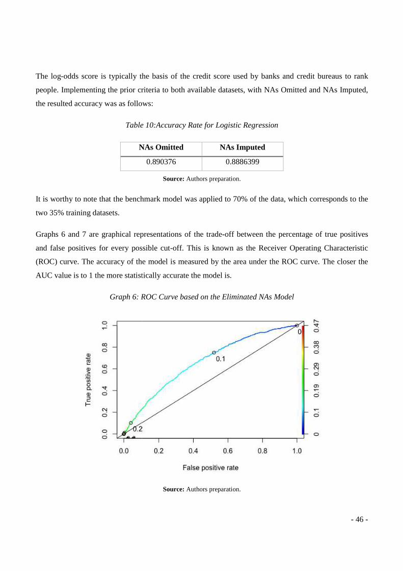
The log-odds score is typically the basis of the credit score used by banks and credit bureaus to rank

people. Implementing the prior criteria to both available datasets, with NAs Omitt

the resulted accuracy was as follows:

Table

NAs Omitted

It is worthy to note that the benchmark model was app

two 35% training datasets.

Graphs 6 and 7 are graphical representation

and false positives for every possible cut

(ROC) curve. The accuracy of the model is measured by the area under the ROC curve. The closer the

AUC value is to 1 the more statistically accurate the model is.

Graph 6: ROC Curve based on the Eliminat

odds score is typically the basis of the credit score used by banks and credit bureaus to rank

Implementing the prior criteria to both available datasets, with NAs Omitt

the resulted accuracy was as follows:

Table 10:Accuracy Rate for Logistic Regression

NAs Omitted NAs Imputed

0.890376 0.8886399


It is worthy to note that the benchmark model was applied to 70% of the data, which corresponds to the

are graphical representations of the trade-off between the percentage of true positives

and false positives for every possible cut-off. This is known as the Receiver Operating Characteristic


AUC value is to 1 the more statistically accurate the model is.

: ROC Curve based on the Eliminated NAs Model


- 46 -

odds score is typically the basis of the credit score used by banks and credit bureaus to rank

Implementing the prior criteria to both available datasets, with NAs Omitted and NAs Imputed,

lied to 70% of the data, which corresponds to the

off between the percentage of true positives

er Operating Characteristic


ed NAs Model

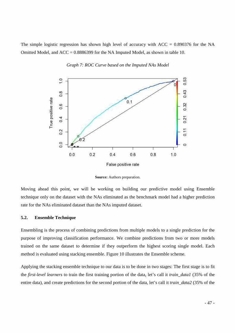
The simple logistic regression has shown high level of accuracy with ACC = 0.890376 for the NA

Omitted Model, and ACC = 0.8886399 for the NA Imputed Model

Graph 7: R

Moving ahead this point, we will be working on building our predictive model using Ensemble

technique only on the dataset with the NAs eliminated as the benchmark model had a higher pre

rate for the NAs eliminated dataset than the NAs imputed dataset.

5.2. Ensemble Technique

Ensembling is the process of combining predictions from multiple models to a single prediction for the

purpose of improving classification performance. We combine

trained on the same dataset to determine if they outperform the highest scoring single model. Each

method is evaluated using stacking ensemble.

Applying the stacking ensemble te

the first-level learners to train the first training portion of the data, let’s call it

entire data), and create predictions for the second portion of the da


Omitted Model, and ACC = 0.8886399 for the NA Imputed Model, as shown in table 10.

: ROC Curve based on the Imputed NAs Model



technique only on the dataset with the NAs eliminated as the benchmark model had a higher pre

rate for the NAs eliminated dataset than the NAs imputed dataset.


purpose of improving classification performance. We combine predictions from two or more models


method is evaluated using stacking ensemble. Figure 10 illustrates the Ensemble scheme.

nsemble technique to our data is to be done in two stages

to train the first training portion of the data, let’s call it

, and create predictions for the second portion of the data, let’s call it

- 47 -


, as shown in table 10.

OC Curve based on the Imputed NAs Model


technique only on the dataset with the NAs eliminated as the benchmark model had a higher prediction


predictions from two or more models


Ensemble scheme.

be done in two stages: The first stage is to fit

to train the first training portion of the data, let’s call it train_data1 (35% of the

ta, let’s call it train_data2 (35% of the

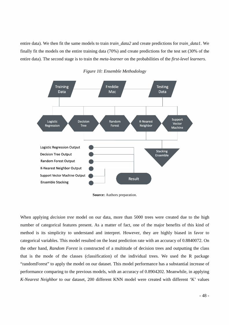
entire data). We then fit the same models to train

finally fit the models on the entire training data (70%) and create predictions for the test set (30% of the

entire data). The second stage is to train the

When applying decision tree model on

number of categorical features present. As a matter of fact, one of the major benefits of this kind of

method is its simplicity to understand and interpret. However, they are highly biased

categorical variables. This model resulted on the least prediction rate with an accuracy of 0.8840072.

the other hand, Random Forest is

that is the mode of the classes (classification) of the indivi

“randomForest” to apply the model on our dataset.

performance comparing to the previous models, with an accuracy of 0.8904202.

K-Nearest Neighbor to our dataset, 200 different KNN model were created with different

We then fit the same models to train train_data2 and create predictions for

inally fit the models on the entire training data (70%) and create predictions for the test set (30% of the

entire data). The second stage is to train the meta-learner on the probabilities of the

Figure 10: Ensemble Methodology


model on our data, more than 5000 trees were created due to the high


method is its simplicity to understand and interpret. However, they are highly biased

iables. This model resulted on the least prediction rate with an accuracy of 0.8840072.

is constructed of a multitude of decision trees and outputting the class

that is the mode of the classes (classification) of the individual trees.

“randomForest” to apply the model on our dataset. This model performance has

performance comparing to the previous models, with an accuracy of 0.8904202.

to our dataset, 200 different KNN model were created with different

- 48 -

and create predictions for train_data1. We

inally fit the models on the entire training data (70%) and create predictions for the test set (30% of the

on the probabilities of the first-level learners.

trees were created due to the high


method is its simplicity to understand and interpret. However, they are highly biased in favor to

iables. This model resulted on the least prediction rate with an accuracy of 0.8840072. On

a multitude of decision trees and outputting the class

dual trees. We used the R package

has a substantial increase of

performance comparing to the previous models, with an accuracy of 0.8904202. Meanwhile, in applying

to our dataset, 200 different KNN model were created with different ‘K’ values

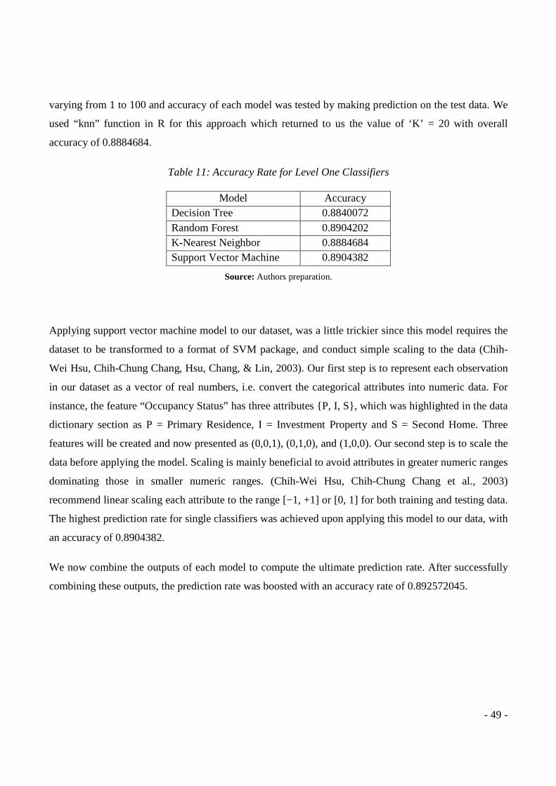
- 49 -

varying from 1 to 100 and accuracy of each model was tested by making prediction on the test data. We

used “knn” function in R for this approach which returned to us the value of ‘K’ = 20 with overall

accuracy of 0.8884684.

Table 11: Accuracy Rate for Level One Classifiers

Model Accuracy Decision Tree 0.8840072 Random Forest 0.8904202 K-Nearest Neighbor 0.8884684 Support Vector Machine 0.8904382


Applying support vector machine model to our dataset, was a little trickier since this model requires the

dataset to be transformed to a format of SVM package, and conduct simple scaling to the data (Chih-

Wei Hsu, Chih-Chung Chang, Hsu, Chang, & Lin, 2003). Our first step is to represent each observation

in our dataset as a vector of real numbers, i.e. convert the categorical attributes into numeric data. For

instance, the feature “Occupancy Status” has three attributes {P, I, S}, which was highlighted in the data

dictionary section as P = Primary Residence, I = Investment Property and S = Second Home. Three

features will be created and now presented as (0,0,1), (0,1,0), and (1,0,0). Our second step is to scale the

data before applying the model. Scaling is mainly beneficial to avoid attributes in greater numeric ranges

dominating those in smaller numeric ranges. (Chih-Wei Hsu, Chih-Chung Chang et al., 2003)

recommend linear scaling each attribute to the range [−1, +1] or [0, 1] for both training and testing data.

The highest prediction rate for single classifiers was achieved upon applying this model to our data, with

an accuracy of 0.8904382.

We now combine the outputs of each model to compute the ultimate prediction rate. After successfully

combining these outputs, the prediction rate was boosted with an accuracy rate of 0.892572045.

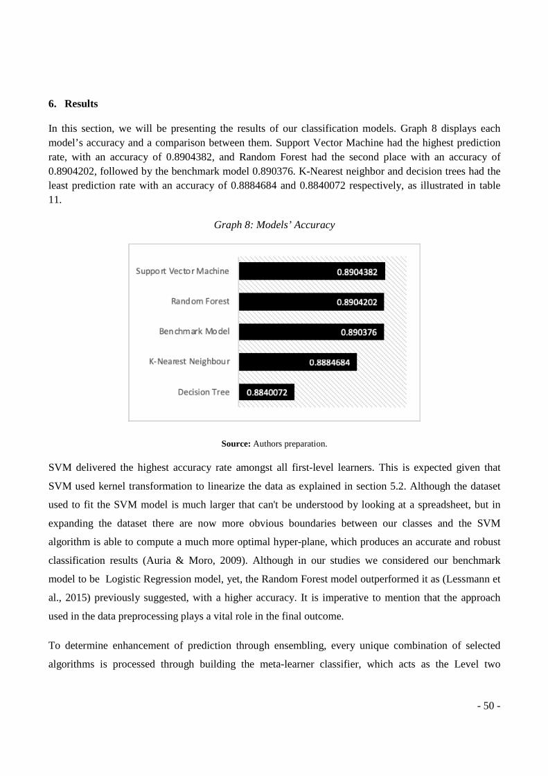
- 50 -

6. Results

In this section, we will be presenting the results of our classification models. Graph 8 displays each model’s accuracy and a comparison between them. Support Vector Machine had the highest prediction rate, with an accuracy of 0.8904382, and Random Forest had the second place with an accuracy of 0.8904202, followed by the benchmark model 0.890376. K-Nearest neighbor and decision trees had the least prediction rate with an accuracy of 0.8884684 and 0.8840072 respectively, as illustrated in table 11.

Graph 8: Models’ Accuracy


SVM delivered the highest accuracy rate amongst all first-level learners. This is expected given that

SVM used kernel transformation to linearize the data as explained in section 5.2. Although the dataset

used to fit the SVM model is much larger that can't be understood by looking at a spreadsheet, but in

expanding the dataset there are now more obvious boundaries between our classes and the SVM

algorithm is able to compute a much more optimal hyper-plane, which produces an accurate and robust

classification results (Auria & Moro, 2009). Although in our studies we considered our benchmark

model to be Logistic Regression model, yet, the Random Forest model outperformed it as (Lessmann et

al., 2015) previously suggested, with a higher accuracy. It is imperative to mention that the approach

used in the data preprocessing plays a vital role in the final outcome.

To determine enhancement of prediction through ensembling, every unique combination of selected

algorithms is processed through building the meta-learner classifier, which acts as the Level two

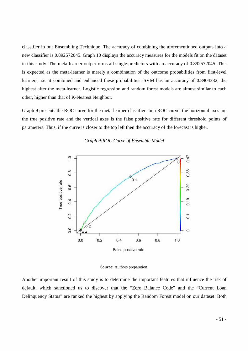
classifier in our Ensembling Technique. The accuracy o

new classifier is 0.892572045. Graph

in this study. The meta-learner outperforms all single predictors

is expected as the meta-learner is merely a combination of the outcome probabilities from first

learners, i.e. it combined and enhanced these probabilities. SVM has an accuracy of 0.8904382, the

highest after the meta-learner. Logistic regression and

other, higher than that of K-Nearest

Graph 9 presents the ROC curve for the meta

the true positive rate and the vertical axes is the fals

parameters. Thus, if the curve is closer to the top left then the accuracy of the forecast is higher.

Graph

Another important result of this study is to determine the important features

default, which sanctioned us to

Delinquency Status” are ranked the highest

classifier in our Ensembling Technique. The accuracy of combining the aforementioned outputs into a

Graph 10 displays the accuracy measures for the models fit on the dataset

learner outperforms all single predictors with an accuracy of 0.892572045

learner is merely a combination of the outcome probabilities from first

, i.e. it combined and enhanced these probabilities. SVM has an accuracy of 0.8904382, the

learner. Logistic regression and random forest models are almost similar to each

Nearest Neighbor.

Graph 9 presents the ROC curve for the meta-learner classifier. In a ROC curve, the horizontal axes

the true positive rate and the vertical axes is the false positive rate for different threshold points of

f the curve is closer to the top left then the accuracy of the forecast is higher.

Graph 9:ROC Curve of Ensemble Model


rtant result of this study is to determine the important features

default, which sanctioned us to discover that the “Zero Balance Code” and the “Current Loan

Delinquency Status” are ranked the highest by applying the Random Forest model on our dataset

- 51 -

f combining the aforementioned outputs into a

displays the accuracy measures for the models fit on the dataset

with an accuracy of 0.892572045. This

learner is merely a combination of the outcome probabilities from first-level

, i.e. it combined and enhanced these probabilities. SVM has an accuracy of 0.8904382, the

random forest models are almost similar to each

In a ROC curve, the horizontal axes are

e positive rate for different threshold points of

f the curve is closer to the top left then the accuracy of the forecast is higher.

rtant result of this study is to determine the important features that influence the risk of

discover that the “Zero Balance Code” and the “Current Loan

t model on our dataset. Both

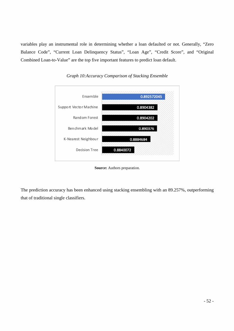
- 52 -

variables play an instrumental role in determining whether a loan defaulted or not. Generally, “Zero

Balance Code”, “Current Loan Delinquency Status”, “Loan Age”, “Credit Score”, and “Original

Combined Loan-to-Value” are the top five important features to predict loan default.

Graph 10:Accuracy Comparison of Stacking Ensemble


The prediction accuracy has been enhanced using stacking ensembling with an 89.257%, outperforming

that of traditional single classifiers.

- 53 -

7. Conclusion

For decades, banking institutions’ main focus is to lend debtors’ money, while these lenders mostly aim

to purchase their dream house with the borrowed money. Banks’ decision on whether to approve or

reject a mortgage application is mostly based on the lenders’ credit score. Credit score is a numerical

expression that represents the borrower’s creditworthiness, which is based on tremendous information

being gathered by financial institutions both on the borrower and the underlying property of the

mortgage. Statistical Modelling played an instrumental role in determining whether a prospective home

owner would default or not. A benchmark model is the logistic regression, due to its interpretability.

Since the revolution of big data, default’s prediction became more and more intriguing area to be

explored, and more sophisticated models were implemented that outperformed the traditional classifier

model logistic regression. This paper is devoted to further enhance the logistic regression model by

implementing a stacking ensemble technique, which is merely combining the outputs of different

sophisticated models, (including Random Forest, K-Nearest Neighbor, Decision Tree, and Support

Vector Machine) and use their probability outcome as an input for the Logistic Regression. Dataset used

in our classification modelling is made publicly available by Freddie Mac.

This paper has been both data-focused and method-focused. Data-focused in the sense that the

prediction models were based solely on mortgage dataset provided by Freddie Mac. Method-focused in

the sense of basically applying stacking ensemble technique to classify mortgages into defaults and non-

defaults loans. Given the data dictionary provided by Freddie Mac, and some data exploratory analysis

techniques, we delve into the structure of both the loan origination and performance datasets as well as

examine the relationship between default rate and certain variables. We implemented some data pre-

processing techniques such as examining the relationship between the default rates and the dataset

variables and construction of a random forest model to determine the variable importance. “Zero

Balance Code”, and the “Current Loan Delinquency Status” have the highest influential role in

determining whether a loan defaulted or not. We then used feature engineering techniques to create a

new classification variable that displays “1” for default loans, and “0” for non-default loans. We

benchmarked our study by applying a logistic regression model to our dataset that yielded in a prediction

accuracy of 88.86% for the dataset with missing observation imputed using mice, versus 89.04% for the

dataset with missing observation omitted. The results confirm that applying machine learning methods

- 54 -

yields better forecast accuracy than traditional single classifier models such as logistic regression. The

prediction accuracy of our stacking ensemble is 89.257% outperforming other models used in our study.

Despite the high accuracy of the meta-learner when compared to that of the first-learners, it is highly

unlikely that this technique would be adopted to replace the commonly used Logistic Regression or

Random Forest in Credit Score Analysis. The foremost reason is that the effort exerted to develop the

model is disproportionate to the return. Although other techniques presented in this paper have a slightly

lower classification power, yet, the ease of deployment would definitely play an instrumental role. In

addition, these models are provided as built-in functions in some libraries that can be used quite

effortlessly in R and Python, or in a drag-and-drop application such as Knime, or SAS Enterprise Miner.

A model that is only slightly better most likely will not lead to a change in paradigm.

The technique presented in this paper is generic, solely based on the variables in the dataset. To produce

a more robust model, it is necessary to engineer some new features including Economical Features

such as “unemployment rate”, “rent ratio” , and “vacant ratio” . Social Features that would strengthen

the model prediction would be “divorce rates”, and “marriage rates”. Financial Feature that could be

included are “Consumer Debt Percentage Change”, and “Mortgage Debt Percentage Change”. These

features might be relevant factors in mortgage defaults prediction. One could therefore further expand

the study to include Survival Analysis. Survival Analysis is a statistical approach to estimate the

expected time for an event to take place, in our case, when the “default” occurs. Another interesting

model to explore is the Cox Proportional Hazard model, which is a method for estimating and analyzing

the impact of several given features until an event happens. Both of these afore mentioned further

research opportunities would allow us to examine the probability of survival and impact of different

variables on the hazard rate. The timing when customers default is an interesting area to investigate

since it can provide the bank with the ability to compute the probability over a customer’s lifetime and

perform profit scoring.

- 55 -

8. References

Addo, P. M., Guegan, D. & Hassani, B. (2018). Credit Risk Analysis Using Machine and Deep Learning Models. SSRN. https://doi.org/10.2139/ssrn.3155047

Altman, N. S. (1992). An introduction to kernel and nearest-neighbor nonparametric regression. American Statistician. https://doi.org/10.1080/00031305.1992.10475879

Auria, L. & Moro, R. A. (2009). Support Vector Machines (SVM) as a Technique for Solvency Analysis. SSRN. https://doi.org/10.2139/ssrn.1424949

Azam, R., Danish, M. & Akbar, S. S. (2012). The significance of socioeconomic factors on personal loan decision a study of consumer banking local private banks in Pakistan. IQRA University.

Bagherpour, A. (2017). Predicting Mortgage Loan Default with Machine Learning Methods.

Banasik, J., Crook, J. N. & Thomas, L. C. (1999). Not if but when will borrowers default. Journal of the Operational Research Society, 50(12), 1185–1190. https://doi.org/10.1057/palgrave.jors.2600851

Bash, E. (2015). Machine Learning with R and H2O. Packt. https://doi.org/10.1017/CBO9781107415324.004

Bellotti, T. & Crook, J. (2009). Support vector machines for credit scoring and discovery of significant features. Expert Systems with Applications, 36(2 PART 2), 3302–3308. https://doi.org/10.1016/j.eswa.2008.01.005

Bolarinwa, A. (2017). Machine learning applications in mortgage default prediction. University of Tampere. Retrieved from http://urn.fi/URN:NBN:fi:uta-201712122923

Breiman, L. (1996). Bagging predictors. Machine Learning, 24(2), 123–140. https://doi.org/10.1007/BF00058655

Breiman, L. (2001). Random forests. Machine Learning. https://doi.org/10.1023/A:1010933404324

Breiman, L., Friedman, J. H., Olshen, R. A. & Stone, C. J. (1984). Classification and Regression Trees. The Wadsworth statisticsprobability series (Vol. 19). https://doi.org/10.1371/journal.pone.0015807

Brown, D. R. (2012). A Comparative Analysis of Machine Learning Techniques For Foreclosure Prediction. Nova Southeastern University. Retrieved from https://nsuworks.nova.edu/gscis_etd/105/

Brown, I. & Mues, C. (2012). An experimental comparison of classification algorithms for imbalanced credit scoring data sets. Expert Systems with Applications, 39(3), 3446–3453. https://doi.org/10.1016/j.eswa.2011.09.033

Bühlmann, P. (2012). Bagging, boosting and ensemble methods. In Handbook of Computational Statistics: Concepts and Methods: Second Edition. https://doi.org/10.1007/978-3-642-21551-3__33

- 56 -

Butaru, F., Chen, Q., Clark, B., Das, S., Lo, A. W. & Siddique, A. (2016). Risk and risk management in the credit card industry. Journal of Banking & Finance. https://doi.org/10.1016/j.jbankfin.2016.07.015

Buuren, S. van & Groothuis-Oudshoorn, K. (2011). mice : Multivariate Imputation by Chained Equations in R. Journal of Statistical Software. https://doi.org/10.18637/jss.v045.i03

Chamboko, R., Bravo, J. M. (2016). On the Modelling of Prognosis from Delinquency to Normal Performance on Retail Consumer Loans. Risk Management 18 (4), 264–287.

Chamboko, R., Bravo, J. M. (2018a). Modelling and forecasting recurrent recovery events on consumer loans. International Journal of Applied Decision Sciences, Vol. 12, No. 3, 271-287.

Chamboko, R., Bravo, J. M. (2018b). Frailty correlated default on retail consumer loans in developing markets. International Journal of Applied Decision Sciences, Vol. 12, No. 3, pp.257–270.

Chamboko, R. & Bravo, J. M. (2018c). A multi-state approach to modelling intermediate events and multiple mortgage loan outcomes. Working Paper, submitted to Journal of Banking and Finance.

Chawla, N. V., Bowyer, K. W., Hall, L. O. & Kegelmeyer, W. P. (2002). SMOTE: Synthetic minority over-sampling technique. Journal of Artificial Intelligence Research. https://doi.org/10.1613/jair.953

Chih-Wei Hsu, Chih-Chung Chang, and C.-J. L., Hsu, C.-W., Chang, C.-C. & Lin, C.-J. (2003). A practical guide to support vector classification. BJU International. https://doi.org/10.1177/02632760022050997

Cieslak, D. A. & Chawla, N. V. (2008). Learning decision trees for unbalanced data. In Lecture Notes in Computer Science (including subseries Lecture Notes in Artificial Intelligence and Lecture Notes in Bioinformatics). https://doi.org/10.1007/978-3-540-87479-9_34

Cortes, C. & Vapnik, V. (1995). Support-Vector Networks. Machine Learning. https://doi.org/10.1023/A:1022627411411

Cox, D. R. (1958). The Regression Analysis of Binary Sequences. Journal of the Royal Statistical Society. Series B (Methodological). https://doi.org/10.1007/BF03180993

Debajyoti Ghosh Roy, Bindya Kohli, S. K. (2013). BASEL I TO BASEL II TO BASEL III. AIMA Journal of Management & Research.

Deng, G. (2016). Analyzing the Risk of Mortgage Default. University of California. Retrieved from https://www.stat.berkeley.edu/~aldous/Research/Ugrad/Grace_Deng_thesis.pdf

Dumitrescu, Elena, Hue, Sullivan, Hurlin, Christophe, Tokpavi, S. (2018). Machine Learning for Credit Scoring: Improving Logistic Regression with Non Linear Decision Tree Effects.

Durand, D. (1941). Risk Elements in Consumer Instalment Financing. (D. Durand, Ed.). National Bureau of Economic Research. Retrieved from http://www.nber.org/books/dura41-1

- 57 -

Efron, B. & Tibshirani, R. J. (1993). An introduction to the bootstrap. Monographs on Statistics and Applied Probability, No. 57. Chapman and Hall, London, 436 p. Monographs on Statistics and Applied Probability. https://doi.org/10.1016/j.foodhyd.2013.10.011

Fawcett, T. (2006). An introduction to ROC analysis Tom. Irbm. Pattern Recognition Letters, Elsevier, 27(8),861-874 https://doi.org/10.1016/j.patrec.2005.10.010

Fitzpatrick, T. & Mues, C. (2016). An empirical comparison of classification algorithms for mortgage default prediction: Evidence from a distressed mortgage market. In European Journal of Operational Research. https://doi.org/10.1016/j.ejor.2015.09.014

Frame, W. S., Fuster, A., Tracy, J. & Vickery, J. (2015). The Rescue of Fannie Mae and Freddie Mac. Journal of Economic Perspectives, 29(2), 25–52. https://doi.org/10.1257/jep.29.2.25

Gong, R. & Huang, S. H. (2012). A Kolmogorov-Smirnov statistic based segmentation approach to learning from imbalanced datasets: With application in property refinance prediction. Expert Systems with Applications. https://doi.org/10.1016/j.eswa.2011.12.011

GROOT, J. DE. (2016). Credit risk modeling using a weighted support vector machine. UNIVERSITEIT UTRECHT.

Guyon, I. & Elisseeff, A. (2003). An Introduction to Variable and Feature Selection. Journal of Machine Learning Research (JMLR). https://doi.org/10.1016/j.aca.2011.07.027

Hand, D. J. (2005). Good practice in retail credit scorecard assessment. Journal of the Operational Research Society, 56(9), 1109–1117. https://doi.org/10.1057/palgrave.jors.2601932

Hand D.J & Jacka S. (1998). Statistics in Finance. Hand D.J. and Jacka S. (eds.) Statistics in finance, Edward Arnold.

Hastie, T., Tibshirani, R. & Friedman, J. (2001). The Elements of Statistical Learning. The Mathematical Intelligencer. https://doi.org/10.1198/jasa.2004.s339

Hernandez-Orallo, J., Flach, P. & Ferri, C. (2011). Brier Curves: a New Cost-Based Visualisation of Classifier Performance. In Proceedings of the 28th International Conference on Machine Learning (ICML).

Ho, T. K. (1995). Random decision forests. In Proceedings of 3rd International Conference on Document Analysis and Recognition (Vol. 1, pp. 278–282 vol.1). https://doi.org/10.1109/ICDAR.1995.598994

Horn, D. M. (2016). Credit Scoring Using Genetic Programming. Nova IMS Universidade Nova de Lisboa.

Jafar Hamid, A. & Ahmed, T. M. (2016). Developing Prediction Model of Loan Risk in Banks Using Data Mining. Machine Learning and Applications: An International Journal. https://doi.org/10.5121/mlaij.2016.3101

- 58 -

Khandani, A. E., Kim, A. J. & Lo, A. W. (2010). Consumer credit-risk models via machine-learning algorithms. Journal of Banking and Finance. https://doi.org/10.1016/j.jbankfin.2010.06.001

King, G. & Zeng, L. (2001). Logistic Regression in Rare Events Data. Political Analysis. https://doi.org/10.1093/oxfordjournals.pan.a004868

Koh, H. C., Tan, W. C. & Goh, C. P. (2006). A Two-step Method to Construct Credit Scoring Models with Data Mining Techniques. International Journal of Business and Information, 1(1), 96–118.

Lessmann, S., Baesens, B., Seow, H. V. & Thomas, L. C. (2015). Benchmarking state-of-the-art classification algorithms for credit scoring: An update of research. European Journal of Operational Research, 247(1), 124–136. https://doi.org/10.1016/j.ejor.2015.05.030

Loh, W. Y. (2014). Fifty years of classification and regression trees. International Statistical Review. https://doi.org/10.1111/insr.12016

Louzada, F., Cancho, V. G., Roman, M. & Leite, J. G. (2012). A new long-term lifetime distribution induced by a latent complementary risk framework. Journal of Applied Statistics, 39(10), 2209–2222. https://doi.org/10.1080/02664763.2012.706264

Machova, K., Puszta, M., Barcak, F. & Bednar, P. (2006). A comparison of the bagging and the boosting methods using the decision trees classifiers. Computer Science and Information Systems. https://doi.org/10.2298/CSIS0602057M

Mamonov, S. & Benbunan-Fich, R. (2017). What Can We Learn from Past Mistakes? Lessons from Data Mining the Fannie Mae Mortgage Portfolio. Journal of Real Estate Research.

Marron, D. (2007). “Lending by numbers”: Credit scoring and the constitution of risk within American consumer credit. Economy and Society, 36(1), 103–133. https://doi.org/10.1080/03085140601089846

Mian, A. & Sufi, A. (2014). House of Debt: How They (and You) Caused the Great Recession, and How We Can Prevent It from Happening Again. The University of Chicago Press. https://doi.org/10.1057/be.2015.4

Pundir, S. & Seshadri, R. (2012). A Novel Concept of Partial Lorenz Curve and Partial Gini Index. International Journal of Engineering Science and Innovative Technology (IJESIT), 1(2), 6. Retrieved from https://pdfs.semanticscholar.org/0349/65b6f11e33e59e6b59eebb7e3cbc2725d0c3.pdf

Quinlan, J. R. (1992). C4.5: Programs for Machine Learning. Morgan Kaufmann San Mateo California. https://doi.org/10.1001/jama.1995.03520250075037

Schapire, R. E., Freund, Y., Bartlett, P. & Lee, W. S. (1998). Boosting the margin: A new explanation for the effectiveness of voting methods. Annals of Statistics. https://doi.org/10.1214/aos/1024691352

- 59 -

Sealand, J. C. (2018). Short-term Prediction of Mortgage Default using Ensembled Machine Learning Models. Slippery Rock University. Retrieved from https://www.researchgate.net/profile/Jesse_Sealand/publication/326518013_Short-term_Prediction_of_Mortgage_Default_using_Ensembled_Machine_Learning_Models/links/5b51de7baca27217ffa788bb/Short-term-Prediction-of-Mortgage-Default-using-Ensembled-Machine-Lea

Smyth, P. & Wolpert, D. (1998). Stacked density estimation. Advances in Neural Information Processing Systems.

Thomas, L., Edelman, D. & Crook, J. (2002). Credit Scoring and Its Applications. Mathematical Modeling and Computation. Society for Industrial and Applied Mathematics. https://doi.org/doi:10.1137/1.9780898718317

Tokpavi, H. S. H. C. S. (2018). Machine Learning for Credit Scoring: Improving Logistic Regression with Non Linear Decision Tree Effects. Retrieved from https://www.researchgate.net/publication/318661593_Machine_Learning_for_Credit_Scoring_Improving_Logistic_Regression_with_Non_Linear_Decision_Tree_Effects?enrichId=rgreq-65273f515fe3e5309ed5c83341701df6-XXX&enrichSource=Y292ZXJQYWdlOzMxODY2MTU5MztBUzo1OTM

Torgo, L. (2016). Data mining with R: Learning with case studies, second edition. Data Mining with R: Learning with Case Studies, Second Edition. https://doi.org/10.1201/9781315399102

Vandell, K. D. (1978). Distributional Consequences of Alternative Mortgage Instruments. Real Estate Economics. https://doi.org/10.1111/1540-6229.00172

Wolpert, D. H. (1992). Stacked generalization. Neural Networks, 5(2), 241–259. https://doi.org/10.1016/S0893-6080(05)80023-1

Zhou, Y. W., Zhong, Y. & Li, J. (2012). An uncooperative order model for items with trade credit, inventory-dependent demand and limited displayed-shelf space. European Journal of Operational Research, 223(1), 76–85. https://doi.org/10.1016/j.ejor.2012.06.012

Zhou, Z.-H. (2012). Ensemble Methods: Foundations and Algorithms. Ensemble Methods: Foundations and Algorithms. https://doi.org/doi:10.1201/b12207-2

Machine Learning Approach For Credit Score Analysis v8 - Final

Documents

Transcript of Machine Learning Approach For Credit Score Analysis v8 - Final