MACHINE LEARNING AND PATTERN RECOGNITION Fall 2004 ...

MACHINE LEARNING AND

PATTERN RECOGNITION

Fall 2004, Lecture 1:

Introduction and Basic Concepts

Yann LeCunThe Courant Institute,New York Universityhttp://yann.lecun.com

Y. LeCun: Machine Learning and Pattern Recognition – p. 1/29

Before we get started...

Course web site: http://www.cs.nyu.edu/ yann/2004f-G22-3033-002/index.html

Evaluation: Assignements (mostly small programming projects) [60%] + largerfinal project [40%].

Course mailing list:http://www.cs.nyu.edu/mailman/listinfo/g22_3033_002_fa04

Text Books: mainly “Pattern Classification” by Duda, Hart, and Stork, but anumber of other books can be used reference material: “Neural Networks forPattern Recognition” by Bishop, and “Element of Statistical Learning” byHastie, Tibshirani and Friedman.

... but we will mostly use resarch papers and tutorials.

formal prerequisite: linear algebra. You might want to brush up on probabilitytheory, multivariate calculus (partial derivatives ...), optimization (least squaremethod...), and the method of Lagrange multipliers for constrainedoptimization. We will review those topics in class.

Programming projects: can be done in any language, but I STRONGLYrecommend to use Lush ( http://lush.sf.net ). Skeleton code in Lush will beprovided for most projects.


What is Learning?

Learning is acquiring and improving performance through experience.

Pretty much all animals with a central nervous system are capable of learning(even the simplest ones).

What does it mean for a computer to learn? Why would we want them to learn?How do we get them to learn?

We want computers to learn when it is too difficult or too expensive to programthem directly to perform a task.

Get the computer to program itself by showing examples of inputs and outputs.

In reality: we will write a “parameterized” program, and let the learningalgorithm find the set of parameters that best approximates the desired functionor behavior.


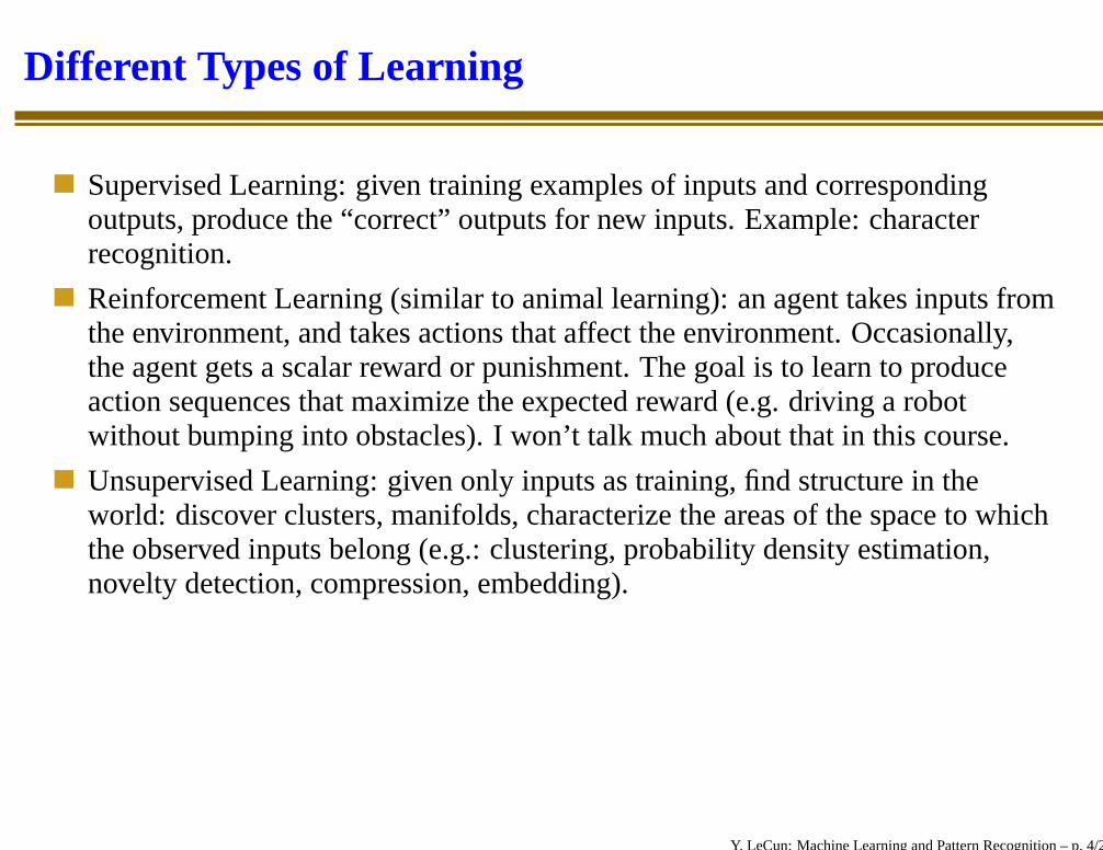
Different Types of Learning

Supervised Learning: given training examples of inputs and correspondingoutputs, produce the “correct” outputs for new inputs. Example: characterrecognition.

Reinforcement Learning (similar to animal learning): an agent takes inputs fromthe environment, and takes actions that affect the environment. Occasionally,the agent gets a scalar reward or punishment. The goal is to learn to produceaction sequences that maximize the expected reward (e.g. driving a robotwithout bumping into obstacles). I won’t talk much about that in this course.

Unsupervised Learning: given only inputs as training, find structure in theworld: discover clusters, manifolds, characterize the areas of the space to whichthe observed inputs belong (e.g.: clustering, probability density estimation,novelty detection, compression, embedding).


Related Fields

Statistical Estimation: statistical estimation attempts to solve the same problemas machine learning. Most learning techniques are statistical in nature.

Pattern Recognition: pattern recognition is when the output of the learningmachine is a set of discrete categories.

Neural Networks: neural nets are now one many techniques for statisticalmachine learning.

Data Mining: data mining is a large application area for machine learning.

Adaptive Optimal Control: non-linear adaptive control techniques are verysimilar to machine learning methods.

Machine Learning methods are an essential ingredient in many fields:bio-informatics, natural language processing, web search and text classification,speech and handwriting recognition, fraud detection, financial time-seriesprediction, industrial process control, database marketing....


Applications

handwriting recognition, OCR: reading checks and zipcodes, handwritingrecognition for tablet PCs.

speech recognition, speaker recognition/verification

security: face detection and recognition, event detection in videos.

text classification: indexing, web search.

computer vision: object detection and recognition.

diagnosis: medical diagnosis (e.g. pap smears processing)

adaptive control: locomotion control for legged robots, navigation for mobilerobots, minimizing pollutant emissions for chemical plants, predictingconsumption for utilites...

fraud detection: e.g. detection of “unusual” usage patterns for credit cards orcalling cards.

database marketing: predicting who is more likely to respond to an ad campaign.

(...and the antidote) spam filtering.

games (e.g. backgammon).

Financial prediction (many people on Wall Street use machine learning).Y. LeCun: Machine Learning and Pattern Recognition – p. 6/29

Demos / Concrete Examples

Handwritten Digit Recognition: supervised learning for classification

Handwritten Word Recognition: weakly supervised learning for classificationwith many classes

Face detection: supervised learning for detection (faces against everything elsein the world).

Object Recognition: supervised learning for detection and recognition withhighly complex variabilities

Robot Navigation: supervised learning and reinforcement learning for control.


Two Kinds of Supervised Learning

Regression: also known as “curve fitting”or “function approximation”. Learn acontinuous input-output mapping from alimited number of examples (possiblynoisy).

Classification: outputs are discrete vari-ables (category labels). Learn a decisionboundary that separates one class from theother. Generally, a “confidence” is also de-sired (how sure are we that the input be-longs to the chosen category).


Unsupervised Learning

Unsupervised learning comes down to this: if the input looks like the training samples,output a small number, if it doesn’t, output a large number.

This is a horrendously ill-posed problem in highdimension. To do it right, we must guess/discoverthe hidden structure of the inputs. Methods differby their assumptions about the nature of the data.

A Special Case: Density Estimation. Find afunction f such f(X) approximates theprobability density of X , p(X), as well aspossible.

Clustering: discover “clumps” of points

Embedding: discover low-dimensional manifoldor surface near which the data lives.

Compression/Quantization: discover a functionthat for each input computes a compact “code”from which the input can be reconstructed.


Learning is NOT Memorization

rote learning is easy: just memorize all the training examples and theircorresponding outputs.

when a new input comes in, compare it to all the memorized samples, andproduce the output associated with the matching sample.

PROBLEM: in general, new inputs are different from training samples.

The ability to produce correct outputs or behavior on previously unseen inputs iscalled GENERALIZATION.

rote learning is memorization without generalization.

The big question of Learning Theory (and practice): how to get goodgeneralization with a limited number of examples.


A Simple Trick: Nearest Neighbor Matching

Instead of insisting that the input be exactlyidentical to one of the training samples, let’scompute the “distances” between the input and allthe memorized samples (aka the prototypes).

1-Nearest Neighbor Rule: pick the class of thenearest prototype.

K-Nearest Neighbor Rule: pick the class that hasthe majority among the K nearest prototypes.

PROBLEM: What is the right distance measure?

PROBLEM: This is horrendously expensive if thenumber of prototypes is large.

PROBLEM: do we have any guarantee that we getthe best possible performance as the number oftraining samples increases?


How Biology Does It

The first attempts at machine learning in the 50’s,and the development of artificial neural networksin the 80’s and 90’s were inspired by biology.

Nervous Systems are networks of neuronsinterconnected through synapses

Learning and memory are changes in the“efficacy” of the synapses

HUGE SIMPLIFICATION: a neuron computes aweighted sum of its inputs (where the weights arethe synaptic efficacies) and fires when that sumexceeds a threshold.

Hebbian learning (from Hebb, 1947): synapticweights change as a function of the pre- andpost-synaptic activities.

orders of magnitude: each neuron has 103 to 105

synapses. Brain sizes (number of neurons): housefly: 105; mouse: 5.106, human: 1010.


The Linear Classifier

Historically, the Linear Classifier was designed as a highly simplified model of theneuron (McCulloch and Pitts 1943, Rosenblatt 1957):

y = f(

i=N∑

i=0

wixi)

With f is the threshold function: f(z) = 1 iffz > 0, f(z) = −1 otherwise. x0 is assumedto be constant equal to 1, and w0 is interpretedas a bias.In vector form: W = (w0, w1....wn), X =(1, x1...xn):

y = f(W ′X)

The hyperplane W ′X = 0 partitions the spacein two categories. W is orthogonal to the hy-perplane.


Vector Inputs

With vector-based classifiers such as the linear classifier, we must represent objects inthe world as vectors.Each component is a measurement or a feature of the the object to be classified.For example, the grayscale values of all the pixels in an image can be seen as a (veryhigh-dimensional) vector.


A Simple Idea for Learning: Error Correction

We have a training set Sconsisting of P input-outputpairs: S = (X1, y1), (X2, y2), ....(XP , yP ).A very simple algorithm:- show each sample in sequence repetitively- if the output is correct: do nothing- if the output is -1 and the desired output +1: increasethe weights whose inputs are positive, decrease theweights whose inputs are negative.- if the output is +1 and the desired output -1: de-crease the weights whose inputs are positive, increasethe weights whose inputs are negative.More formally, for sample p:

wi(t + 1) = wi(t) + (ypi − f(W ′Xp))xp

i

This simple algorithm is called the Perceptron learn-ing procedure (Rosenblatt 1957).


The Perceptron Learning Procedure

Theorem: If the classes are linearly separable (i.e. separable by a hyperplane), thenthe Perceptron procedure will converge to a solution in a finite number of steps.Proof: Let’s denote by W ∗ a normalized vector in the direction of a solution. Supposeall X are within a ball of radius R. Without loss of generality, we replace all Xp

whose yp is -1 by −Xp, and set all yp to 1. Let us now define the marginM = minpW

∗Xp. Each time there is an error, W.W ∗ increases by at leastX.W ∗ ≥M . This means Wfinal.W

∗ ≥ NM where N is the total number of weightupdates (total number of errors). But, the change in square magnitude of W isbounded by the square magnitude of the current sample Xp, which is itself boundedby R2. Therefore, |Wfinal|2 ≤ NR2. combining the two inequalities

Wfinal.W∗ ≥ NM and |Wfinal| ≤

√NR, we have

Wfinal.W∗/|Wfinal| ≥

√

(N)M/R

. Since the left hand side is upper bounded by 1, we deduce

N ≤ R2/M2


Good News, Bad News

The perceptron learning procedure can learn a linear decision surface, if such asurface exists that separates the two classes. If no perfect solution exists, theperceptron procedure will keep wobbling around.What class of problems is Linearly Separable, and learnable by a Perceptron?There are many interesting applications where the data can be represented in a waythat makes the classes (nearly) linearly separable: e.g. text classification using “bag ofwords” representations (e.g. for spam filtering).Unfortunately, the really interesting applications are generally not linearly separable.This is why most people abandonned the field between the late 60’s and the early 80’s.We will come back to the linear separability problem later.


Regression, Mean Squared Error

Regression or function approximation is finding afunction that approximates a set of samples as wellas possible.Classic example: linear regression. We aregiven a training set S of input/output pairs S =

{(X1, y1), (X2, y2)....(XP , yP )}, and we must findthe parameters of a linear function that best predictsthe y’s from the X’s in the least square sense. In otherwords, we must find the parameter W that minimizesthe quadratic loss function L(W,S):

L(W,S) =1

P

P∑

i=1

L(W, yi, Xi)

where the per-sample loss function L(W, yi, Xi) is defined as:

L(W, yi, Xi) =1

2(yi −W ′Xi)2


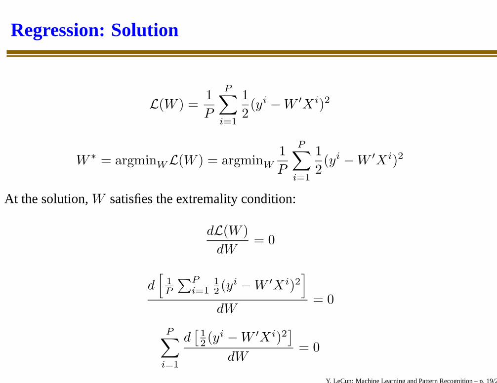
Regression: Solution

L(W ) =1

P

P∑

i=1

1

2(yi −W ′Xi)2

W ∗ = argminWL(W ) = argminW

1

P

P∑

i=1

1

2(yi −W ′Xi)2

At the solution, W satisfies the extremality condition:

dL(W )

dW= 0

d[

1P

∑P

i=112 (yi −W ′Xi)2

]

dW= 0

P∑

i=1

d[

12 (yi −W ′Xi)2

]

dW= 0


A digression on multivariate calculus

W : a vector of dimension N . W ′ denotes the transpose of W , i.e. if W isN × 1 (column vector), W ′ is 1×N (line vector).

F (W ): a multivariate scalar-valued function (an N -dimensional surface in anN + 1 dimensional space).

dF (W )

dW=

[

∂F (W )

∂w1,∂F (W )

∂w2, . . .

∂F (W )

∂wN

]

is the gradient of F (W ) with respect to W (it’s a line vector).

The gradient of a function that maps N -dim vectors scalars is a 1×N linevector.

example 1: linear function: F (W ) = W ′X where X is an N -dim vector:d(W ′X)

dW= X ′

example 2: quadratic function F (W ) = (y −W ′X)2 where y is a scalar:d(y−W ′X)2

dW= −2(y −W ′X)X ′.


Regression: Solution

The gradient of L(W) is:

dL(W )

dW=

P∑

i=1

d[

12 (yi −W ′Xi)2

]

dW=

P∑

i=1

−(yi −W ′Xi)Xi′

The extremality condition becomes:

1

P

P∑

i=1

−(yi −W ′Xi)Xi′ = 0

Which we can rewrite as:

[

P∑

i=1

yiXi

]

−[

P∑

i=1

XiXi′

]

W = 0


Regression: Direct Solution

P∑

i=1

yiXi − [

P∑

i=1

XiXi′]W = 0

Can be written as:

[P

∑

i=1

XiXi′]W =P

∑

i=1

yiXi

This is a linear system that can be solved with a number of traditional numericalmethods (although it may be ill-conditioned or singular).

If the covariance matrix A =∑P

i=1 XiXi′ is non singular, the solution is:

W ∗ =

[

P∑

i=1

XiXi′

]−1P

∑

i=1

yiXi


Regression: Iterative Solution

Gradient-based minimization: W (t + 1) = W (t)− η dL(W )dW

where η is a well chosen coefficient (often a scalar, sometimes diagonal matrix withpositive entries, occasionally a full symmetric positive definite matrix).The k-th component of the gradient of the quadratic loss L(W ) is:

∂L(W )

∂wk

=

P∑

i=1

−(yi −W (t)′Xi)xik

If η is a scalar or a diagonal matrix, we can write the udpate equation for a single

component of W : wk(t + 1) = wk(t) + η∑P

i=1(yi −W (t)′Xi)xi

k

This update rules converges for well-chosen, small-enough values of η (more on thislater).


Regression, Online/Stochastic Gradient

Online gradient descent, aka Stochastic Gradient:

W (t + 1) = W (t)− ηd(W, Y i, Xi)

dW

wk(t + 1) = wk(t) + η(t)(yi −W (t)′Xi)xik

No sum! The average gradient is replaced by its instantaneous value.This is called stochastic gradient descent. In many practical situation it isenormously faster than batch gradient.But the convergence analysis of this method is very tricky.One condition for convergence is that η(t) must be decreased according to a schedulesuch that

∑

t η(t)2 converges while∑

t η(t) diverges.One possible such sequence is η(t) = η0/t.We can also use second-order methods, but we will keep that for later.


Least Mean Squared Error for Classification

We can use the Mean Squared Error criterion witha linear regressor to perform classification (althoughthis is clearly suboptimal).We compute a linear discriminant functionG(W, X) = W ′X and compare it to a threshold T .If G(W, X) is larger than T , we classify X in class1, if it is smaller than T , we classify X n class 2.

To compute W , we simply minimize the quadratic loss function

L(W ) =1

P

P∑

i=1

1

2(yi −W ′Xi)2

where yi = +1 if training sample X i is of class 1 and yi = −1 if trainingsample Xi is of class 2.

This is called the Adaline algorithm (Widrow-Hoff 1960).


Linear Classifiers

In multiple dimensions, the linear discriminant function G(W, X) = W ′X partitionsthe space into two half-spaces separated by a hyperplane.


A Richer Class of Functions

What if we know that the process that generatedour samples is non linear? We can use a richerfamily of functions, e.g. polynomials, sum oftrigonometric functions....PROBLEM: if the family of functions is too rich,we run the risk of overfitting the data. If the fam-ily is too restrictive we run the risk of not beingable to approximate the training data very well.QUESTIONS: How can we choose the richnessof the family of functions? Can we predict the per-formance on new data as a function of the trainingerror and the richness of the family of functions?Simply minimizing the training error may not giveus a solution that will do well on new data.


Learning as Function Estimation

pick a machine G(W, X) parameterized by W . Itcan be complicated and non-linear, but it better bedifferentiable with respect to W .

pick a per-sample loss function L(Y, G(W, X)).

pick a training setS = (X1, Y 1), (X2, Y 2), ....(XP , Y P ).

find the W that minimizesL(W,S) = 1

P

∑

i L(Y i, G(W, Xi))


Learning as Function Estimation (continued)

If L(Y i, G(W, Xi)) is differentiable with respect toW , use a gradient-based minimization technique:

W ←W − η∂L(W )

∂W

or use a stochastic gradient minimization technique:

W ←W − η∂L(Y i, G(W, Xi))

∂W


MACHINE LEARNING AND PATTERN RECOGNITION Fall 2004 ...

Documents

Transcript of MACHINE LEARNING AND PATTERN RECOGNITION Fall 2004 ...