1

MACH Rocketry Spring 2020 Report

Luke Egbert, Team Lead

Jamie Weiss, Team Lead

Adam DeCino

TC Della Penna

Kian Roybal

Trevor Toft

2

Abstract In Spring 2017, we launched our first rocket for this project. The first rockets were

hobby store Estes kits and quickly after these first launches, we were launching our first high

power rockets to obtain certifications that would allow us to fly larger, more powerful

rockets. After 18 months of flying rockets and learning all we could, we began planning for

our proof of concept rocket in late Spring 2019. This rocket was to be a data acquisition tool

that would allow us to see how well our designs translated into the real world and how well

our software predicted the flight. During the Summer 2019 we wrote a MATLAB code to

predict the rocket flight which included supersonic airflow and coefficient of drag

calculations well beyond Mach. The test rocket went to 35,300 ft and Mach 2.0 as predicted

by the software. This flight also proved that our other designed components functioned as

well; these included fins, ejection charges, motor closures, and the nozzle. After this success

we were ready to move forward with the larger design and planning started in August 2019.

This rocket was originally planned to reach Mach 4.5 at 30,000 ft and then proceed to an

altitude of over 300,000 ft. Unfortunately, due to budgetary restrictions, we were forced to

scale back the project and optimize the design for weight and speed. We took what we could

from the rocket that we launched and began to redesign. The simulations said that the rocket

would reach over 65,000 ft and Mach 3.0. At these speeds and altitudes special

considerations must be made, including fin geometry/vibration, surface area reduction, rigid

motor to air frame attachment, and high-altitude ejection charges. As we began design of

these components we simultaneously designed and tested a new, more energetic propellant.

We optimized the fins for the minimum surface area, minimum weight, and the highest

possible Mach number without the fins vibrating apart. By weight reducing the coupling

3

mechanism we were able to reduce its weight by almost 50% over the previous design and

still maintain rigidity. High-altitude ejection charges were tested in a custom built vacuum

chamber with a pressure sensor and a variety of charges were tested so we could obtain the

most desirable results. The launch date for this rocket has been pushed back due to

unforeseen circumstances, but we do plan on flying it as soon as possible.

4

Table of Contents

Abstract ..................................................................................................................................................................... 2

List of Figures ......................................................................................................................................................... 6

List of Tables ........................................................................................................................................................ 10

Introduction ......................................................................................................................................................... 11

Launch from BALLS 28 .................................................................................................................................... 12

Original and Modified Design ........................................................................................................................ 13

Motor Hardware ............................................................................................................................................ 14

Motor Casing .................................................................................................................................................... 15

Original Fins ..................................................................................................................................................... 16

Modified Fins ................................................................................................................................................... 18

Ejection Charges ............................................................................................................................................. 21

Original Forward Closure ........................................................................................................................... 22

Modified Forward Closure ......................................................................................................................... 24

Launch Tower ................................................................................................................................................. 25

Motor Mixing and Testing ............................................................................................................................... 28

Formula X Characterization ........................................................................................................................... 29

Original Final Motor .......................................................................................................................................... 31

Modified Final Motor ........................................................................................................................................ 32

Nozzle Analysis and Design ............................................................................................................................ 38

Original Final Nozzle .................................................................................................................................... 41

Modified Final Nozzle .................................................................................................................................. 42

Machining and Analysis ................................................................................................................................... 46

Materials Testing ................................................................................................................................................ 51

Materials Selection ............................................................................................................................................ 53

Analysis .................................................................................................................................................................. 59

Original Simulation Output ............................................................................................................................ 73

Program Architecture....................................................................................................................................... 76

Results ................................................................................................................................................................ 77

Discussion of Program ................................................................................................................................. 80

Pressure Transducer ........................................................................................................................................ 81

5

Discussion of Code ........................................................................................................................................ 81

Conclusion............................................................................................................................................................. 82

References ............................................................................................................................................................ 83

Appendices ........................................................................................................................................................... 84

Rocket Basic Sim MATLAB Code .............................................................................................................. 84

Distributed Mass Properties Program ................................................................................................... 95

Arduino Pressure Transducer Code ..................................................................................................... 101

6

List of Figures Figure 1: 8-inch diameter final rocket.

Figure 2: 5:1 Von Karman 8-inch nose cone for final rocket.

Figure 3: Cross sectional view of final rocket.

Figure 4: This model was run at 150% the expected maximum pressure and has a safety

factor of 2. Analysis of the closures and attachment of the closures will still need to be done

in the future.

Figure 5: The two rockets simulated in Open Rocket have a stability that is very close to the

same, but the second rocket has a 10% reduction in surface area resulting in lower drag.

Figure 6: Old fin with new fin cut away.

Figure 7: Fin analysis and divergent Mach number.

Figure 8: Brass tee charge that is used for high altitude ejection.

Figure 9: Forward closure for final rocket.

Figure 10: Exploded view of airframe components.

Figure 11: New design for coupling flange.

Figure 12: Model of lower tower section with motor tube.

Figure 13: View of tower rails supporting the motor tube.

Figure 14: Pressure vs Time for one of the test burns.

Figure 15: Burn Rate vs Chamber Pressure graph to calculate a and n.

7

Figure 16: The 3D printed casting bases.

Figure 17: Grains curing.

Figure 18: Grain length, propellant diameter, and core size. Total length of propellant is 48

inches.

Figure 19: The blue curve is thrust in pounds, the green curve is pressure in psi, the pink

curve is mass flux in lb/s-in2, and the red curve is Kn.

Figure 20: Outputs from BurnSim.

Figure 21: Thrust vs Time curve from motor test.

Figure 22: Pressure vs Time curve from motor test.

Figure 23: Picture of test burn.

Figure 24: Current Tripoli N research record.

Figure 25: Coupler used for airframe to motor case connection on a 4-inch rocket.

Figure 26: Analysis done on the coupler used for the BALLS 28 rocket.

Figure 27: New concept of coupler designed to match motor OD to the airframe OD.

Figure 28: Analysis of stress and displacement under 1000 lb compressive load.

Figure 29: Stress/Strain curves for the three carboard tubes, D = 101.6 mm, tested in

compression.

Figure 30: Stress/Strain curves for the three blue phenolic tubes, D = 101.6 mm, tested in

compression.

8

Figure 31: Flowchart of the basic operation in Basic_Rocket_Sim.m.

Figure 32: The basic forces on the rocket represented in Equations (5) & (6).

Figure 33: Motor profile from http://www.thrustcurve.org/simfilesearch.jsp?id=332.

Figure 34: The fit, data points and calculated Mach numbers used in the simulation.

Figure 35: The velocity vs. vertical acceleration graph.

Figure 36: The vertical acceleration vs. time comparison.

Figure 37: Thrust comparison between nominal and adjusted calculations within the

simulation.

Figure 38: The velocity vs. time comparison.

Figure 39: The Displacement vs. time comparison from a launch altitude of 1642.68 [m].

Figure 40: The angular displacement vs. time comparison.

Figure 41: Free body diagram of forces at a given section height of the rocket.

Figure 42: Max Acceleration and Max Velocity calculations from simulation.

Figure 43: Mass flow over time to be checked with thrust curve.

Figure 44: Thrust curve over time to be checked with mass flow curve.

Figure 45: LV-Haack profile with X-axis of symmetry.

Figure 46: Zoomed view of the LV-Haack profile with X-axis of symmetry.

Figure 47: List of mass property results of LV-Haack nose cone as solve by SolidWorks.

9

Figure 48: Resulting volume of LV-Haack nose cone as solve by program.

10

List of Tables Table 1: Calculations of Kn for ballistic test motor.

Table 2: The inputs are Kn, pressure, burn rate and isp* is the output.

Table 3: Grain number with their lengths, weights, and calculated density.

Table 4: 1 inch nozzle throat with 15° convergent angle and 15° divergent angle.

Table 5: 1 inch nozzle throat with 15° convergent angle and 18° divergent angle.

Table 6: 1 inch nozzle throat with 15° convergent angle and 23° divergent angle.

Table 7: Compression of mechanical properties for standard carboard tubing with D = 101.6

mm.

Table 8: Compression of mechanical properties for blue phenolic tubing with D = 101.6 mm.

Table 9: Compression of mechanical properties for fiberglass tubing with D = 101.6 mm.

Figure 10: Comparison of maximum allowable thrust in Newtons for three different

materials.

Table 11: Flight statistics comparison.

Table 12: Calculations and program inputs.

11

Introduction Rocketry is something that we have been doing since the beginning of 2017 and it is

exciting now that we are working towards such a large goal with the biggest rocket we have

ever built. Going through design and analysis has been very important since we started

getting into higher power rockets with very large amounts of thrust. There are many factors

that can affect a rockets flight from, drag, to atmospheric conditions, to stability of the rocket

and so on. Taking these things into account into our simulation program that we designed

will be very helpful in predicting our rocket’s flight.

Getting the opportunity to launch our 4-inch sub-minimum diameter rocket at BALLS

28 was very important in determining what kind of design we were going to pursue forward

with. Since the design worked so well, and the flight went excellent, we wanted to upscale

the rocket, but due to budgetary restrictions, we had to scale the project back. The motor

was also a very important aspect of that flight because we fully tested and characterized the

propellant and launched the largest motor that we had ever mixed. Working on the

propellant for so long has taught us a lot about the way it behaves and the way that we want

to modify it for the final rocket. Machining the aluminum coupler between the motor casing

and the payload was vital because we were able to do finite element analysis on it and knew

that it would withstand the flight that it was going to undergo.

Analyzing not only the flight but the material selection has been very beneficial. We

have tested three different kinds of materials that are used to make rockets and by a large

margin filament wound fiberglass is the strongest and the one that we have been using, and

will continue to use, for these high impulse flights. We wanted to wind our own fiberglass

12

and test those samples to see how they compare to the off the shelf fiberglass, but due to

campus closing we were going to use off the shelf fiberglass instead.

A simulation method was developed to aid the rocketry design process. Routines have

been programmed as needed to obtain mass properties for the distinct sections of a rocket.

This MATLAB procedure will take in known geometries of the rocket and return their

calculated mass values. Most notably, this software will work in reverse and take in an

allowed mass as input and solve for an optimal nose cone thickness. This thickness is not

arbitrary and will provide the cross-sectional area that satisfies the maximum allowable

stress along with its safety factor. This procedure is tentative and to be developed and

updated as the selected material mass-properties are researched.

Launch from BALLS 28 We attended BALLS 28 on the Black Rock Desert in Nevada from September 20-22,

2019. We prepared over the Summer and start of the Fall 2019 semester and launched a 4-

inch sub-minimum diameter rocket on an experiment N3300 to an altitude of 35,300 feet

and 1550 mph. The casing, fin can, fiberglass, and electronics were off the shelf, but the

motor, electronics bay, and aluminum coupler were manufactured by the team. The motor

was an 8 grain 98 mm made from the Purple Pig propellant and had about 3300 N of average

thrust, 14,000 N-s of impulse, and a 3.7 second burn time. The length of the grains near the

forward closure were shorter than the grains near the nozzle because of the high L/D of the

motor. The grains were also stepped with a larger core near the nozzle to account for the

erosive burning that would have happened if the grains were not stepped. Erosive burning

happens when the diameter of the core of the grain is too close to the diameter of the nozzle

13

throat and the exhaust gases as they are ejected erodes the nozzle. The launch was very

successful and allowed us to fly a similar model to what we are building for senior design.

Original and Modified Design Design of the final rocket will be influenced heavily by testing that we have yet to

conduct and data that we have collected from previous rocket launches. The summer

project for the BALLS 28 launch gave a lot of good data and worked as a proof of concept

for a scaled down version of the final rocket that we plan to launch.

Figure 1: 8-inch diameter final rocket.

It will be necessary to test at least two motors on our way to building the big motor

for the final rocket. The tip of the nose cone we plan on building out of titanium and

stainless steel since the tip will experience the most heat and the fiberglass would be at a

high risk of delamination at that point. The nose cone will be filament wound fiberglass

using the X winder and will double as our payload section where the parachutes, cameras,

and electronics will be housed. The forward closure of the motor will double as the

14

mounting point for the nose cone/payload and will be heavily influenced by the rocket we

flew at BALLS 28. The motor casing closures will be secured using grub screws due to their

low profile allowing for better aerodynamics. The nozzle will be made from graphite and

the carrier will be made from aluminum. They will be secured using the same grub screws

as used to secure the forward closure. The fins will be made of aluminum and we will affix

them directly to the motor casing in a way that will not affect the temper of the aluminum.

Figure 2: 5:1 Von Karman 8-inch nose cone for final rocket.

Motor Hardware Designing two casings that are incremental steps towards what we want to do will

be necessary. We will use these motors to test the pressures and temperatures that we can

expect to see in the final motor. For everything up to this point we have been using

standard snap ring casings and casting tubes/liners so building these cases will be very a

new challenge and will prepare us for the final case we need to build. We will also be using

a new technique with these larger motors called case bonding. This technique adheres the

propellant to the inside of the case with some kind of protective layer in between the

15

propellant and the case so the case does not burn through. Both the screw in closures and

case bonding are expandable to a motor of whatever size we want to build and are in fact

very similar to how NASA builds the solid boosters.

From the aft end forward, the grub screws are holding in the nozzle carrier, there

are three fins affixed to the motor casing, the forward closure is being held in by grub

screws as well, and the nose cone has the stepped metal tip.

Figure 3: Cross sectional view of the final rocket.

Motor Casing The motor casing is the largest component of both the airframe and motor. This

cylinder must withstand the internal pressure of the motor and the longitudinal forces

exerted as the rocket travels into large Mach numbers. Fortunately, the internal pressure of

the motor and the pressure on the front end of the motor casing will be opposite each other

and the aluminum casing will be more than strong enough for the compressive forces. The

internal pressure is going to be the main force that we are concerned about. This pressure,

in combination with the temperature rise, due to the motor burning inside, will be a large

16

issue that we must face. For the time being, we will use FEA in SolidWorks for simulating the

pressure. Figure (4) is a standard length of tubing that has a standard wall thickness, and it

is showing more than strong enough for this flight.

.

Figure 4: This model was run at 150% the expected maximum pressure and has a safety factor

of 2. Analysis of the closures and attachment of the closures will still need to be done in the

future.

This will also be done to find the strength of the closures. The closures will be made

from aluminum and will have strength comparable to the rupture strength of the cylinder.

In this case we will design the “weakest” point to be the nozzle end, so we may control the

potential failure mode. The thinking behind this is that if the motor over-pressurizes then

the nozzle will shoot out and the rocket will be mostly undamaged. This will allow recovery

to still work and data from the flight computer to still be collected.

Original Fins The design for the fins will continue to change as the rocket comes together, but the

principles that we use to design them will remain constant. For these very large velocities

17

many things must be considered. If the fins are tall, extending far from the motor casing, then

they could begin to vibrate until they fail and come off the rocket. Extra area also increases

drag, so making the fins as small as possible will be very important. The current thinking is

that by taking the fin design that we have been using and moving the fin tip aft this will allow

for the center of pressure of the fin to also move back and maximize the fin’s effect on the

center of pressure of the rocket. This has the added benefit of allowing us to make the fins

have a smaller surface area and be shorter, solving all the issues we are faced with. The fin

designs will be designed in Open Rocket and then put into a fin simulation software to find

the maximum speed that we can fly with the proposed design. This software is commercial

and finds the velocity that the fin will begin to vibrate at. In Figure (5) we can see that the

effect of pulling the area as far back as possible can have similar results to the stability with

a smaller area.

18

Figure 5: The two rockets simulated in Open Rocket have a stability that is very close to the

same, but the second rocket has a 10% reduction in surface area resulting in lower drag.

Modified Fins When it comes to fins, the design must account for the high temperature, high

windspeed, and high frequency vibration. They will have the largest area towards the back

to maximize effect of shifting CP. They will be made of aluminum that is affixed to the

motor casing. Aluminum will be the best choice for fin material due to its high melting point

and relatively low weight. Further analysis will determine theoretical maximum

temperatures we can expect on the leading edge of the fins. Aluminum will be able to

withstand the temperature better than the composite alternative. Also, the high velocities

that we are aiming for will cause some issues including vibration in the fins that could

cause the fins to fail. Making the fins shorter and closer to the body of the rocket will

increase the resonance frequency and increase the velocity that this velocity would occur

at. We will also need to find the theoretical best shape for the fins using subsonic testing in

the wind tunnel. These shapes that we test will also be tested in commercial fin flutter

software at our target velocity. From these tests we will find the fin shape that gives the

best efficiency with the lowest chance of flutter. Also, designing the fins to have the largest

effect on CP per unit surface area will help determine the fin sizing. This will be the largest

factor in designing the rocket and will account for the loss of propellent throughout the

burn. Aiming for an initial stability of between 1.2 to 1.8 calibers (rocket diameters) we will

be able to size the fins to get the exact stability that we want during the powered portion of

the flight.

19

The fins have been complicated to analyze because of complexities in the harmonics

of the fins and how they resonate with velocity. Depending on the fin geometry, attachment

method to the rocket, and the material, the flutter velocity will change. The flutter velocity

is the resonance frequency of the fins, and how the fins interact with the air as they pass

through the fluid. As the Mach number rises, the air behaves more and more as a viscous

fluid. This interaction becomes important for our fin design when the Mach number

reaches greater than 2. This rocket will go faster than Mach 3 so this will be analyzed with

the available tools. We will primarily be using the FinSim software to do this analysis. The

reason for this software is that the interactions between the velocity and the resonance

frequency is beyond the scope of our undergrad degree. Having said this, the fins that we

used for the BALLS rocket this last year were a very robust design for the vibration, but the

fin design is not very efficient. A different fin design will be necessary for a faster and more

efficient rocket. To make an efficient fin the center of pressure must be as far back on the

fin as possible, because the center of pressure of the entire rocket is so heavily dependent

on the fins. This means that similar to affecting the center of gravity of a system of masses

on a bar by moving a mass further away and therefore increasing the lever arm for that

mass and increasing its impact on the whole system. The center of pressure can be seen in

the same way, as a series of center of pressures, all with some lever arm from the total

center of pressure. This means that by moving the fins backwards that they will have a

greater impact on the CP per unit area. That being said, we are looking for a shape that has

the smallest area but the largest impact on the center of pressure. The design that we have

settled for is a convenient shape that we can take from the existing fin can, that we know is

easily capable of withstanding high velocity. We will modify the fins to get this shape.

20

Figure 6: Old fin with new fin cut away.

This new fin will reduce the surface area by 11% and has a more efficient design for

the actual shape. Also, it will lighten the rocket by reducing the size of the fin and reducing

the length of the fin can.

Fin simulation software shows that with the new fin design that the fins will flutter

at a Mach number of 4.74 and the ultimate failure velocity will be 6.45. These numbers are

not 100% accurate, but they do give an estimate and a confidence. They show that the fins

should be fine at a much higher Mach number than we will function at. These numbers will

also be in an idealized situation and any perturbance will cause a greater deformation in

the fins. Also, the rocket will encounter some angle of attack and the force on the fins will

be larger than predicted by the software. This will be compensated for by having a

substantial safety factor in terms of velocity.

21

Figure 7: Fin analysis and divergent Mach number.

Ejection Charges These charges will be what actually separates the rocket at apogee, and this alone

will require many hours of testing. The rapid creation of gas is the goal of the charges, but

many things will affect our gas production rate and efficiency. The altitude will be the

largest hurdle to overcome and this is why we plan on building a vacuum chamber to

simulate the high atmosphere. This will allow us to make and test as many charges and

types of gas generation that we want to. From what we have researched, tested, and flown,

black powder will be our most likely candidate. These Black Powder charges will be housed

in machined “charge wells” that will contain the gasses and burning powder for long

22

enough for a full combustion of powder to take place. We will test various shapes to find

the smallest size that is able to achieve full combustion.

Figure 8: Brass tee charge that is used for high altitude ejection charges.

Original Forward Closure The forward closure must be simple in design, robust, and light weight. We are

looking at making the forward closure and coupler section to the nose cone in one part.

This part will need to hold pressure and withstand a substantial heat during the thrust

phase, along with being the attachment point for the nose cone/ payload section. This will

23

be more light weight and allow for a very secure connection between the nose cone and

motor. This will also be a bolt on or “Frankenstein” attachment style and will have a

forward ring similar to the rocket launched at BALLS recently. This design did well

practically and was easy enough for us to manipulate in the rocket. This shows that a well

thought out and thoroughly simulated part will also be successful in a larger rocket.

Figure 9: Forward closure for the final rocket.

24

Modified Forward Closure We also have a new design for the coupling flange that serves to attach the airframe to the

motor. The new design is 325 grams lighter than the part used for the BALLS launch and has

adequate strength to withstand a 300lbf side load. The fiberglass will be made with a slightly

smaller diameter than the BALLS airframe. This is to eliminate the transitional area between

the motor tube and the airframe. We have built a mandrel out of MDF in order to make

sections of airframe for testing. Our hope is that we will be able to match the strength of

factory parts.

Figure 10: Exploded view of airframe components.

25

Figure 11: New Design of Coupling Flange

The FEA of the coupling flange was done with a 300 lbf transverse load applied. This

load was estimated based on the data given by our simulation of the 8-inch motor. This

analysis will be updated as soon as we are able to process the data gathered at the most

recent motor test.

Launch Tower We began working on some of the elements of support and logistics that will be

necessary for us to launch. We have built a pressure chamber with a pressure transducer

which we plan to test ejection charges in. We have also designed a launch tower and have

begun the process of applying for a waiver with the FAA and finding a launch location.

The launch tower will guide the rocket in the first moments of the launch until the

rocket becomes stable. The design we came up with utilizes off-the-shelf materials for

26

construction and will be able to adjust for various airframe diameters. The tower will have a

fixed external frame that supports adjustable internal rails that will guide the rocket. We will

build the frame and rails out of Unistrut and accessory brackets as well as 3/8 all thread.

There will be a bottom and a top section of the tower, each 10 feet tall and connected with

four-hole brackets. A model of the bottom section is shown in figure (12) with a model of an

8 inch motor tube.

Figure 12: Model of lower tower section with motor tube.

27

Figure (12) is a view of the lower section showing the three rails supporting the motor

tube as well as the tubular rings which will give the tower added rigidity.

Figure 13: View of tower rails supporting the motor tube.

Stakes will be driven through three holes in the base of the tower. For additional

support, each frame member will have a 3/16-inch stainless steel cables as guy wires at the

midpoint and top of the section. The top section of the tower will have additional guy wires

at the midpoint and top. Some changes to the current design may be going from rings to

hexagons in order to make manufacturing easier and faster. We also have plans for

increasing the stiffness between the outer frame and inner rails using tubing.

28

Motor Mixing and Testing Over the course early to mid-2019, we worked on characterizing a propellant.

Characterizing a propellant means that you start off with a formula, and you make grains, to

then test them in a motor and see what the data looks like. We mixed many batches of a

formula we got from Brad McGarvey called Purple Pig. The first few batches were all 54 mm

grains that we used in 2, 3, and 4 grain motors. All were successful burns, but the chamber

pressure was lower than we wanted it to be. We were running a pressure of about 150 – 250

psi where most propellants run closer to 1000 psi. The next grains we mixed were for

another 54 mm, a 75 mm, and a 98 mm. The 54 mm was a 2 grain with a different sized nozzle

to allow us to obtain a higher chamber pressure. The 75 mm was a 3 grain and the 98 mm

was a 2 grain. After those tests, we were able to characterize the propellant because we had

enough data. The first program that was used was ProPep 3 which is a program where you

input the formula and then all the information about the grains, and it calculates a burn rate

coefficient and a burn rate exponent. Those numbers are needed for the next program that

is used which is called BurnSim. In BurnSim, your propellant gets entered and you can enter

the grains and the nozzle dimensions so you can test the propellant. BurnSim outputs a

thrust curve, the ISP, the impulse, mass flow, and burn time. BurnSim can be used to verify

the data from your test burns and it can also be used to make larger motors and see what

their burn will look like. From the test burn data, we learned that the propellant was not as

energetic as we would have liked it to be, so we plan on modifying the propellant over the

next few months. The process of characterizing a propellant was invaluable and it will allow

us to characterize a new one much more efficiently.

29

Formula X Characterization After BALLS 28, we decided we needed a more energetic propellant to be able to

achieve our goals. We started working on new formulas and talking with experienced people

in rocketry and developed a formula that we think is the best for our situation. We spent a

week mixing small batches to try to figure out the ratio of liquids to the curative so we would

have complete cure. Then we made five pucks with a propellant diameter of 2.88 inch and a

length of 1.00 inch. We were lent a ballistic evaluation motor which was a thick-walled

cylinder with closures and a spot for interchangeable nozzles. We machined nozzles with

different core diameters and no divergent or convergent cones. We wanted to have five

different nozzles so we could have five different Kn values.

𝐾𝑛 =𝑎𝑟𝑒𝑎 𝑜𝑓 𝑏𝑢𝑟𝑛𝑖𝑛𝑔 𝑝𝑟𝑜𝑝𝑒𝑙𝑙𝑎𝑛𝑡 𝑠𝑢𝑟𝑓𝑎𝑐𝑒

𝑎𝑟𝑒𝑎 𝑜𝑓 𝑛𝑜𝑧𝑧𝑙𝑒 𝑡ℎ𝑟𝑜𝑎𝑡 (1)

Table (1) shows what the values of Kn are based on the nozzle throat.

Table 1: Calculations of Kn for ballistic motor.

Propellant

Diameter [in]

Nozzle

Throat [in]

Area Propellant

[in2]

Area

Nozzle [in2]

Kn

2.88 0.1875 6.514 0.0276 235.9296 2.88 0.1719 6.514 0.0232 280.7757 2.88 0.1563 6.514 0.0192 339.7386 2.88 0.1406 6.514 0.0155 419.4304 2.88 0.1250 6.514 0.0123 530.8416

After running the five test burns in the ballistic motor, we sorted through the data and

plotted pressure vs time. One of the burn graphs is shown in figure (14).

30

Figure 14: Pressure vs Time graph for one of the test burns.

To find the average pressure over the course of the burn the square wave portion is analyzed.

To find the burn rate the “turn on” and “turn off” are found and the two times are subtracted,

and the length of the grain is divided by the time. Once the burn rate is found, the propellant

can be characterized. Table (2) represents the inputs to calculate the isp* and figure (15)

represents the output.

Table 2: The inputs are Kn, pressure, burn rate and isp* is the ouput.

Kn psi burn rate isp*

Test 1 235.9296 489.6478 0.1251 255.1356

Test 2 280.7757 495.1629 0.1419 191.1766

Test 3 339.7386 581.1354 0.1515 173.7100

Test 4 419.4304 762.8155 0.1564 178.9174

Test 5 530.8416 889.6208 0.1577 163.5285

0

1000000

2000000

3000000

4000000

5000000

6000000

7000000

8000000

9000000

0 2 4 6 8

Pre

ssu

re (

Pa)

Time (s)

31

Figure (15) is a logarithmic plot to find the burn rate coefficient (a) and the burn rate

exponent (n).

Figure 15: Burn Rate vs Chamber Pressure graph to calculate a and n.

Once the a and n are found they can be put into Burnsim and any motor can now be

designed, and the results will be very accurate.

Original Final Motor The 8 inch motor was designed in Burnsim and we scaled it down for a 4 and 6 in test.

Over Fall Break, 60 pounds of propellant was mixed, and casting tube and liner was ordered.

We have both the 4 and 6 inch cases and we will be able to pour the grains and test early in

the new year. It will be a great test of the new propellant and it will also be good to look at

the thrust and pressure data from the tests and compare it to Burnsim and see if anything

needs to be tuned to fit how the actual propellant is performing.

y = 0.0821x0.0964

0.14

0.145

0.15

0.155

0.16

0.165

0.00 200.00 400.00 600.00 800.00 1000.00 1200.00 1400.00

Bu

rn R

ate

(IP

S)

Chamber Pressure (PSI)

32

Modified Final Motor After the characterization of Formula X, we realized that this propellant liked high Kn

numbers, so we knew we wanted to test the motors at a higher Kn as well. Initially, we were

going to test a 4 inch, a 6 inch, and then fly the 8 inch. Due to limitations in our budget, we

had to scale back. We decided that we were going to fly the same rocket that we flew at BALLS

28 but with the new, more energetic propellant. We also were going to focus on making the

rocket as optimized as possible. After discussing the possibility of different test stand burns

we decided we just wanted to test the 4 inch motor which is the same motor that we are

going to fly.

The motor was entered into BurnSim and a nozzle throat was chosen based on the

pressures. We decided that the profile BurnSim created was what we were looking for and

cast the grains based on the dimensions that we had entered into BurnSim. We decided to

3D print casting bases so we could create a dishing on one end of each of the grains to create

and standoff so the flame front can get in between each of the grains. This is a traditional

Bates grain geometry and usually O-rings are used as a standoff between grains, but we

wanted to see if we could create a dishing that would work.

33

Figure 16: The 3D printed casting bases.

Figure 17: Grains curing.

34

After the grains were cast, we weighed and measured all the grains to see how they

compared to each other. We also calculated a density of each grain and averaged it to get the

overall density of the propellant.

Table 3: Grain numbers with their lengths, weights, and calculated density.

grain # core dia CT ID grain L

predicted weight

Recorded weight

[g]

Weight in lbs -

CT Calculated

density

1 1.25 3.24 4 0.745 0.744 1.5927 0.05674 2 1.25 3.24 4 0.745 0.744 1.5927 0.05674 3 1.25 3.24 4 0.745 0.742 1.5883 0.05658 4 1.25 3.24 4 0.745 0.744 1.5927 0.05674 5 1.315 3.24 7.875 1.439 1.442 3.0854 0.05689 6 1.315 3.24 7.9375 1.450 1.456 3.1155 0.05700 7 1.66 3.24 7.9375 1.280 1.292 2.7539 0.05706 8 1.66 3.24 8 1.291 1.316 2.8061 0.05769

Below are the characteristics of the motor along with the curves and outputs.

Figure 18: Grain length, propellant diameter, and core size. Total length of the propellant is 48

inches.

35

Figure 19: The blue curve is thrust in pounds, the green curve is pressure in psi, the pink curve

is mass flux in lb/s-in2, and the red curve is Kn.

Figure 20: Outputs from BurnSim.

Once the data was received from the test, we were able to sort through it. As we have

noticed with other motors that we have tested, BurnSim was conservative with the

simulation. It is hard to figure out which number is driving why the theoretical does not align

with the actual test burn, so the numbers need to be played with until BurnSim aligns better

with the actual results. Sometimes, it is not possible to get it to fully resemble the actual

motor and that is why testing is necessary to prove how the motor is performing.

36

Figure 21: Thrust vs Time curve from motor test.

Figure 22: Pressure vs Time curve from motor test.

Looking at the difference of the test stand data versus BurnSim it is apparent that the

thrust curve is not what BurnSim predicted it would look like. It is similar, and they are both

relatively flat burns, but this curve is ever so slightly regressive instead of ever so slightly

0

1000

2000

3000

4000

5000

6000

0 1 2 3 4 5 6

Th

rust

(N

)

Time (s)

0

1000000

2000000

3000000

4000000

5000000

6000000

7000000

0 1 2 3 4 5 6

Pre

ssu

re (

Pa)

Time (s)

37

progressive. Both curves do produce a good square wave portion and we were very happy

with how the motor performed. After going through the data the burn time was 5.56 sec, the

average pressure was 664 psi with a peak pressure of 864 psi, the average thrust was 3326

N, and the total impulse was 18,527 Ns. The motor is a 90% N3300.

Figure 23: Picture of test burn.

Since this is such a large N, we decided we are going to try for the Tripoli Research

Record. The current record is 31,580 feet which we exceeded that altitude already at BALLS

28 with 35,300 feet.

38

Figure 24: Current Tripoli N research record.

Since we did not state we were going for a record then we were not allowed to claim it.

According to the simulations, our rocket will exceed 60,000 feet so we had to apply for a

unique FAA waiver. We plan on flying out at the Mojave Desert with Friends of Amateur

Rocketry from April 25-26, 2020. The process of applying for the waiver was straightforward

once we knew for sure that the rocket was considered a Class 2 rocket since the motor is

under the P impulse range. The waiver was applied for on February 19, 2020 and we have

been in contact with the FAA since then.

Nozzle Analysis and Design In the early phases of MACH Rocketry, our team has experimented with different

nozzle sizes during test burns and other high-power flights. Iterations of tests were

completed to ensure that the most efficient nozzle would be used for our final design. This

derived from computing chamber pressures generated by the ignition and burning of the

propellant and the throat diameter of the nozzle. Our first test burns of the propellant

designed and characterized by our team showed a low chamber pressure which resulted in

a small amount of thrust. By decreasing the throat diameter of the nozzle, the chamber

pressure will increase, creating a more powerful thrust out of the rocket and ultimately

propelling it to higher altitudes.

39

In order to properly design and test rocket nozzles, it is important to understand the

theory behind the part. The nozzle is designed to take hot gases and exert them out the

opposite direction of desired flight as fast as possible. This forces the rocket to fly directly up

at extreme speeds. The solid rocket propellant, sitting stationary in the casing, is ignited and

the fuel is burned creating hot gases that need a place to escape. The nozzle is designed to let

those gases flow smoothly into the entrance and then through the nozzle throat. The nozzle

then diverges into a larger diameter. This geometry allows the hot gases to exert force on the

nozzle walls and the mass flow rate to speed up beyond Mach 1.0. The ideal nozzle pressure

will equal the atmospheric pressure at the exit of the nozzle cone, creating a rectangle-like

shape of mass being exerted out the aft end and forcing the rocket forward at its most

efficient rate. The dimensions of the nozzle are crucial to this effect and will be calculated

and characterized for our final rocket design.

Our team began by testing rocket motors on a smaller scale in order to ensure the fuel

mixture was mixed appropriately and would successfully burn. Once the data from these test

burns was gathered and analyzed, the process was repeated on a larger scale. After multiple

tests, the fuel was completely characterized, and the rocket motor was ready for flight. The

nozzle dimensions were determined following this process given the chamber pressure data.

The initial tests of the smaller motors produced low pressures around 200 psi. This needed

to increase in order to produce a large amount of thrust. The nozzle throat was then

decreased to 1.172 in. to restrict the mass flow rate entering the convergent section of the

nozzle and increasing the Mach number in the divergent section. The chamber pressure of

the motor for BALLS 28 was about 650 psi according to BurnSim which was suitable for our

40

launch. The flight was successful, and the motor produced a total impulse of approximately

14,000 N-s, and 742 lbs of average thrust.

The future design of the rocket will be on a much larger scale and therefore will need

a significantly larger amount of thrust. The nozzle will be crucial in determining the correct

amount of thrust needed. The design of the nozzle will consist of a 6 in cylindrical piece of

graphite, which will then be machined, creating the convergent and divergent sections. The

nozzle will be held in place by nozzle carrier group. The outside diameter will fit directly into

the inside diameter of the rocket motor casing. The nozzle carrier group will be machined

out of 6061 T6 Aluminum and will be held in by 6 set screws placed evenly around the

cylindrical shape. The nozzle will fit inside the carrier group, ensuring the nozzle will not be

forced out of the aft end of the rocket during flight. There are a few considerations when

designing the nozzle and nozzle carrier. The main consideration will be the thermal

expansion properties of graphite and aluminum. If they expand at different enough rates

then the nozzle could become dislodged in the carrier, causing the thrust to be affected.

Another consideration for this design is the quality of the graphite. There are many different

qualities of graphite that can be purchased from manufactures. These include, very fine, fine,

and rough. Each quality has advantages and disadvantages, and these must be considered

when designing the nozzle. The rough graphite is the most cost beneficial but the lowest

quality. The very fine is the most expensive of all the options but has the finest detail. These

design limitations are crucial to the performance of the rocket nozzle and will be considered

in the final design.

41

In order to ensure the best nozzle design for the rocket there will be iterations of

testing and machining. Our team will be purchasing a smaller diameter section of graphite

to machine and test in a rocket motor. Before the machining process begins, the team will

test a 3-D model in SolidWorks using the flow simulation tool. This will give the team

valuable data for entrance length, throat diameter, throat length, and exit length. Following

computational analysis, the team will machine the nozzle and test the product in a motor

burn test. Solidifying the machining process and gathering critical data, our team will be able

to move forward with the final nozzle design.

Original Final Nozzle The nozzle is a critical element to the final performance of the rocket and has been

analyzed extensively. The geometry of the nozzle is crucial to its performance and that has

been the main design concern. From the propellant testing, certain characteristics have been

determined such as Kn values, chamber pressures, burn time and Cp/Cv values. We have

created a program to calculate the throat diameter of the nozzle from these values. The rest

of the rocket nozzle dimensions can be calculated from knowing the diameter of the throat.

This is essential to ensuring maximum performance of the rocket in its final launch. We are

going to start manufacturing of the nozzles the week of finals. This will be the first step in

the chain to creating the nozzle for the final rocket. The first nozzle will be 4 inches in

diameter and will be used in a motor test, the next nozzle will be 6 inches and will be used in

a motor test as well, and the final nozzle will be manufactured to be used in the final rocket.

The final 8 inch diameter rocket will utilize a nozzle carrier design that will reduce the

amount of graphite used and will save money and weight. The nozzle will be bolted into an

aluminum hollow carrier to ensure that it stays in the rocket during maximum acceleration.

42

The nozzle carrier will have a boat tail design incorporated to decrease aerodynamic drag

on the rocket.

Modified Final Nozzle A new nozzle configuration was determined to be essential to the success of the final

flight. Multiple iterations of geometries were tested using an online simulator. The theory

behind the geometry was established and researched before advancing onto the testing and

machining of the part. There were a few concerns with the design of the nozzle geometry

including the pressure of the chamber that the nozzle throat creates and the over/under

expansion and actual performance and thrust.

The chamber pressure is crucial to the performance of the rocket. This pressure is

directly related to the propellant and the nozzle throat dimensions. After running multiple

simulations it was determined that the nozzle throat would be 1 inch in diameter. With the

new formula for the propellant, this diameter would create a chamber pressure of

approximately an average of 700 psi. This is a semi-conservative approach for our rocket.

After the most recent motor test the results show a maximum chamber pressure of 864 psi

and an average pressure of 664 psi. This is a positive result of the test but can be improved

by approximately 100 psi. Simulations were performed in order to determine the new nozzle

throat. The new nozzle throat will be more restricting and will have a diameter of 0.97 inches.

Expansion is directly related to the performance of the nozzle and thrust which will

ultimately enhance the performance of the rocket. A study of expansion was conducted using

the nozzle simulator. This study evaluates the performance of the nozzle using three

different geometries. The results are shown below.

43

Table 4: 1 inch nozzle throat with 15° convergent angle and 15° divergent angle.

Altitude Thrust Isp State feet lbf sec 1000 930.01 242.6 UnderExpanded 2000 941.72 243.3 UnderExpanded 3000 953.43 244.0 UnderExpanded 4000 965.13 244.7 UnderExpanded 5000 976.84 245.4 UnderExpanded 6000 988.11 245.9 UnderExpanded 7000 999.82 246.6 UnderExpanded 8000 1011.09 247.1 UnderExpanded 9000 1022.36 247.7 UnderExpanded 10000 1033.63 248.2 UnderExpanded 11000 1045.77 248.9 UnderExpanded 12000 1056.61 249.3 UnderExpanded 13000 1068.10 249.9 UnderExpanded 14000 1079.15 250.3 UnderExpanded 15000 1089.15 250.5 UnderExpanded

MACH # at exit = 2.78 Avg Thrust = 1010.73 lbf Avg Isp = 247.0 sec Max Thrust = 1089.15 lbf Thrust Coefficient (Cf) = 1.64 (At max thrust)

Table 5: 1 inch throat with 15° convergent angle and 18° divergent angle.

Altitude Thrust Isp State feet lbf sec 1000 936.158 244.2 UnderExpanded 2000 948.78 245.1 UnderExpanded 3000 961.411 246.1 UnderExpanded 4000 974.04 247 UnderExpanded 5000 986.66 247.9 UnderExpanded 6000 998.716 248.6 UnderExpanded 7000 1011.342 249.4 UnderExpanded 8000 1023.395 250.2 UnderExpanded 9000 1035.448 250.8 UnderExpanded 10000 1047.5 251.5 UnderExpanded 11000 1060.7 252.5 UnderExpanded

44

12000 1072.179 253 UnderExpanded 13000 1084.519 253.7 UnderExpanded 14000 1096.285 254.3 UnderExpanded 15000 1106.674 254.5 UnderExpanded

MACH # at exit = 2.96

Avg Thrust = 1022.92 lbf

Avg Isp = 249.9 sec

Max Thrust = 1106.67 lbf

Thrust Coefficient (Cf) = 1.659 (At max thrust)

Table 6: 1 inch nozzle throat with 15° convergent angle and 23° divergent angle.

Altitude Thrust Isp State feet lbf sec 1000 933.389 243.5 OverExpanded 2000 947.286 244.7 OverExpanded 3000 961.183 246 OverExpanded 4000 975.08 247.2 OverExpanded 5000 988.977 248.4 OverExpanded 6000 1002.096 249.4 OverExpanded 7000 1015.993 250.6 OverExpanded 8000 1029.113 251.5 UnderExpanded 9000 1042.232 252.5 UnderExpanded 10000 1055.351 253.4 UnderExpanded 11000 1070.026 254.7 UnderExpanded 12000 1082.367 255.4 UnderExpanded 13000 1095.875 256.3 UnderExpanded 14000 1108.606 257.1 UnderExpanded 15000 1119.47 257.4 UnderExpanded

MACH # at exit = 3.16

Avg Thrust = 1028.47 lbf

Avg Isp = 251.2 sec

Max Thrust = 1119.47 lbf

Thrust Coefficient (Cf) = 1.659 (At max thrust)

45

The altitude shown in the first column in the three tables is determined from the burn

time of the rocket. This is an approximation given that the burn time will be around 5.5 to 6

seconds. It is clear from these results that the largest exit cone angle of 23° has the optimal

performance. The thrust is the largest of the three geometries as well as the mach number at

the exit of the nozzle. The expansion was also shown for each of the scenarios and it was

determined that the data from Table (6) had the best expansion ratios. The optimal

performance for any nozzle would have a parallel plume out of the exit of the nozzle giving

it a perfectly expanded ratio. In the final geometry of 23° divergent cone angle, the expansion

is almost perfectly parallel throughout the majority of the burn. This will produce the highest

amount of thrust and will be completely optimized for the final flight.

As discussed earlier, a motor test was conducted to test the new propellant formula

as well as the 1 inch nozzle throat with a 15° convergent cone angle and divergent cone angle.

The nozzle was machined out of superfine isomolded graphite using the lathe. The cylinder

was cut to length and then machined down to the correct outside diameter. The first step to

cut the inside geometry was to bore out the nozzle throat diameter all the way through the

cylinder of graphite. Once this step was accomplished, the entrance cone was machined. The

lathe was set at the appropriate angle and we began cutting in and then reversing the cut

outwards. This step was repeated until the exit diameter was the correct dimension. The

nozzle was then flipped around and chucked up to begin cutting the entrance cone. This was

much longer of a process and took multiple passes. Once the entrance diameter dimension

was met, the sanding and polishing process began. We started with 800 grit sandpaper at

typical rotating lathe machining speeds and with my finger, carefully pressed the sandpaper

onto the inside surface of the graphite nozzle. After multiple passes, we switched to 1000

46

grit sandpaper, repeating the same steps. The final polish was created using 1500 grit

sandpaper and pressing with a great amount of force on the inside surface of the nozzle. This

removed any leftover grit on the graphite and created a polished surface finish. This is

essential to achieving the optimal performance of the nozzle as well as making post clean up

processes easier.

The nozzle performed very well during the motor test. The new nozzle will contain

the updated geometry with a 23° divergent cone angle with a 0.97 inch throat diameter.

Machining of the new nozzle will begin shortly and will be the final nozzle for the final rocket.

Machining and Analysis The objective of this project dictates that we minimize the effects of aerodynamic drag

on the rocket. We decided to try a sub-minimum diameter design to reduce both the weight

and drag caused by a larger diameter airframe. In order to eliminate the lower portion of the

rocket which typically incorporates the fins, a motor tube and centering rings, we designed

a coupler that makes the connection between the upper airframe and the motor case. We

built and launched a rocket as a proof of concept for the design using a 4-inch airframe and

motor case. The coupler that we manufactured can be seen in Figure (25).

47

Figure 25: Coupler used for airframe to motor case connection on a 4-inch rocket.

This design has a 1.5-inch sleeve which slips down over the top of the motor case. The

sleeve caused a step in the outer diameter (OD) of the rocket between the airframe and the

motor case. The inner diameter (ID) of this sleeve was machined to match the OD of the

motor case with a 0.002-inch clearance. The idea was to minimize the movement between

the coupler and the motor to increase the stability of the assembly. The motor case sits flush

against a 0.25-inch thick ring that transmits the force of thrust to the rest of the airframe.

Analysis of this ring under a 1100 lb. compressive load gave a safety factor (S.F.) of greater

than 19. Although a lower S.F. would reduce the weight of the part and increase the altitude

of the rocket, strength was our concern for this build. The next iteration will be better

optimized to decrease the weight of the part and still maintain a reasonable S.F.

48

Figure 26: Analysis done on the coupler that was used for the BALLS 28 rocket.

A lathe was used to turn the top 6 inches of the coupler down to match the inner diameter of

the fiberglass coupler which in turn slid into the fiberglass section of airframe. The inner

fiberglass coupler was unnecessary and will likely be revised in the next design evolution to

save weight. Both the bottom and top IDs were machined using the same process.

49

A solid 6061-T6 aluminum cylinder was faced on both ends to ensure a perpendicular

surface. The center of the cylinder was then drilled to a 1-inch ID using several drills of

increasing diameter. A boring bar was then used to take the ID out to the final desired

dimension. Once the inner and outer diameters had been machined our next operation was

to drill and tap holes in the upper portion. These holes were tapped with 8-32 threads and

were used to attach the fiberglass airframe to the coupler. Windows were machined out of

the walls of the coupler using a 0.5-inch end mill to reduce weight.

The design of the final rocket will use a similar method for attaching the airframe to

the motor case. The most notable difference with the new design is that the coupler is

incorporated into the forward closure of the motor. This is made possible by designing the

forward closure with a different method of retention. The previous rocket used a retaining

ring in a groove cut into the inside of the motor tube to keep the forward closure in place.

The new motor will have a series of set screws threaded into the forward closure, allowing

the top of the forward closure to be flush with the top of the motor tube. This feature will

allow us to match the OD of the airframe to the OD of the motor case without a stepped or

tapered transition. This should aid in reducing the aerodynamic drag and reduce the

possibility of bow-shock at the different OD’s.

50

Figure 27: New concept of coupler designed to match the motor OD to the airframe OD.

The new design shown in Figure 19 incorporates rigid fingers which will be bolted to

the forward closure. The fingers will be offset from the OD of the forward closure so that the

OD of the fiberglass airframe matches the OD of the motor case. Analysis of these fingers

under a 1100 lb. compressive load yielded a maximum normal stress of 1626.57 psi and a

maximum displacement of 1.7 × 10−5 inches. The forces applied for this analysis were

estimated using the thrust applied by the 4-inch rocket. The thrust of the final rocket should

be much greater however the load will be distributed to the fiberglass airframe directly with

this design. This will allow us to decrease the thickness of the web on the supports. The

purpose of the fingers will be to add support in the event of a moment being applied to the

airframe. For this reason, it may be necessary to increase the number of supports.

51

Figure 28: Analysis of stress and displacement under 1100 lb. compressive load.

Materials Testing High power rocketry requires a thorough evaluation of engineering topics including

aerodynamics, propellant characterization, nozzle design, electronics, and material design.

Material testing and evaluation is crucial to ensuring a successful flight under extreme

compressive loads. The purpose of this test was to determine the mechanical properties of

multiple materials in hollow cylindrical form to augment and enhance the design of the body

tube on our rocket. The three materials, standard cardboard, blue phenolic, and fiberglass

tubing, were placed under compression until fracture and the mechanical properties were

recorded. These properties were analyzed, and important specifications were calculated to

determine the optimum body tube material. The compressive strength of fiberglass, 175.14

MPa, outperformed the other materials by an excellent margin. This value was evaluated and

determined to withstand an average thrust value of 90018.35 N. It was determined that

fiberglass is the best material for high power rocketry and our design.

52

There are many aspects to building and designing a rocket. To enhance the

performance in each of these categories, the designer must consider the materials necessary.

In this portion, material design and testing will be evaluated and discussed. Our team, MACH

Rocketry, conducted compression tests on multiple materials to determine the best possible

material for our body tube. This can improve strength, aerodynamics and save weight,

ultimately achieving a greater altitude. The purpose of this test was to determine the

mechanical properties of multiple materials in hollow cylindrical form to augment and

enhance the design of the body tube on our rocket.

This test consisted of three separate materials to be evaluated under compression.

The materials will be standard cardboard tubing, phenolic tubing commonly referred to as

blue tube, and filament wound fiberglass.

The compression tests were conducted using the Instron Machine as well as the

certified MTP concrete compression tester. The pre-processing of the materials included

cutting down an original 4 feet length tube of each of the materials into smaller sample sizes.

The tubes were cut down into 6 in lengths with each material consisting of 4 in diameter

sections. The ends of the cylinders were sanded down to ensure a flat contact surface for the

testing devices. The exact lengths, inside diameter, and outside diameters were measured

before conducting the compression test. The cross-sectional area was then calculated using

equation (2) to record and calculate the stress later on.

𝐴𝑐 = 𝜋 ∗ (𝑂𝐷2−𝐼𝐷2

4) (2)

Where OD is the outside diameter of the tubing and ID is the inside diameter of the tubing.

Once these values were calculated and recorded, the samples were ready to test. The Instron

53

was used for the first two samples, the standard cardboard tube and the blue phenolic tubing.

The Instron was calibrated and the sample was placed into the machine. The software was

set to record the extension in millimeters and load in Newtons. The extension rate on the

machine was set to 2 mm/min which was later determined too slow and was increased to 10

mm/min. The safety stop on the Instron was set to 25 kN to ensure that if the sample

exceeded the limits of the machine, the load cell would not malfunction and break. The heads

of the Instron were lowered to right above the sample and then using the small increment

adjustment, brought down flush with the top of the sample. The loads were then balanced

on the software and the protective door was closed. The compression test was then

conducted until the sample failed and the data was recorded. This process was repeated

multiple times for a total of 6 samples, three for each material. The fiberglass was then placed

into the Instron and tested in compression. The material was too strong for the machine,

exceeding the 25 kN load cell, and was determined that it must be tested in a larger, more

powerful machine. Our team decided to use the MTP concrete compression testing machine.

The samples of fiberglass were placed in the machine and the steel heads were placed on the

top and bottom of the sample. The machine was calibrated and began compressing the

material. Once the material had failed, the samples were removed carefully, being aware of

any fiberglass splinters, and evaluated further.

Materials Selection Following the testing of the materials under compression, the data was analyzed, and

the mechanical properties were calculated. The results from the compression test of

standard 4-inch diameter (𝐷 = 101.6 𝑚𝑚) cardboard, blue phenolic, and fiberglass tubing

are shown below in Tables 1, 2, and 3 respectively.

54

Table 7: Comparison of mechanical properties for standard cardboard tubing with D = 101.6 mm.

Table 8: Comparison of mechanical properties for blue phenolic tubing with D = 101.6 mm.

Table 9: Comparison of mechanical properties for fiberglass tubing with D = 101.6 mm.

Given these results and from the calculations of stress and strain from the compression tests

of each material, plots were created to show the relationship between stress and strain for

the given materials. These plots are shown below for the cardboard and blue phenolic tubing.

Sample Length [mm]

Thickness [mm]

Area [mm2]

Compressive Strength

[MPa]

Elastic Modulus

[MPa]

1 151.84 2.06 323.38 10.54 1540.51

2 151.12 1.91 300.26 10.64 1683.60

3 152.76 2.06 323.05 11.05 1354.45

Mean 151.91 2.01 315.56 10.74 1526.20

Std. Dev 0.82 0.09 13.25 0.27 165.02

Sample Length [mm]

Thickness [mm]

Area [mm2]

Compressive Strength

[MPa]

Elastic Modulus

[MPa]

1 152.40 4.57 715.98 24.78 2460.91

2 151.23 3.25 516.66 29.54 2327.43

3 150.93 3.71 577.63 25.92 2505.15

Mean 151.52 3.84 603.42 26.75 2431.16

Std. Dev 0.78 0.67 102.13 2.49 92.52

Sample Length [mm]

Thickness [mm]

Area [mm2]

Compressive Strength

[MPa]

Elastic Modulus

[MPa]

1 152.88 3.61 568.86 162.57 6480.16

2 152.12 3.25 513.81 175.14 5116.59

3 152.70 3.40 537.62 157.20 2454.83

Mean 152.57 3.42 540.10 164.97 4683.86

Std. Dev 0.40 0.18 27.61 9.21 2047.26

55

The fiberglass was tested in the Instron initially but unfortunately, maxed out the 25 kN load

cell’s capabilities. Due to this, our team tested the fiberglass samples in the concrete

compression machine which only produced a total load applied value. A plot for the

fiberglass samples is not available, at this time. Future samples will be wound on the filament

winder and tested appropriately, and plots will be created for these results. The compression

tests produced the load in Newtons and the deformation in millimeters and from this raw

data, the stress and strain can be calculated. The stress is calculated using equation (3).

𝜎 =𝐹

𝐴𝑐 (3)

Where 𝜎 is the stress in MPa, 𝐹 is the load applied to the part in Newtons, and 𝐴𝑐 is the cross-

sectional area of the sample in millimeters. The strain can then be calculated using equation

(4) below.

𝜀 =𝐿 − 𝐿0

𝐿0 (4)

Where 𝜀 is the strain in [mm/mm], 𝐿 is the length of the sample after deformation has

occurred in millimeters, and 𝐿0 is the original length of the sample in millimeters. These

values were plotted and shown below for the cardboard and blue phenolic tubing in Figures

1 and 2 respectively.

56

Figure 29: Stress/Strain curves for three cardboard tubes, D = 101.6 mm, tested in

compression.

0

2

4

6

8

10

12

14

16

18

20

0 0.005 0.01 0.015 0.02 0.025 0.03 0.035 0.04 0.045 0.05

Stre

ss [

MP

a]

Strain [mm/mm]

Cardboard Compression Test

Sample 1

Sample 2

Sample 3

57

Figure 30: Stress/Strain curves for three blue phenolic tubes, D = 101.6 mm, tested in

compression.

A comparison of compressive strength and thrust was calculated to show the maximum

allowable thrust that each material can withstand. The tabulated results are shown below in

Table 10.

Table 10: Comparison of maximum allowable thrust in Newtons for three different materials.

0

5

10

15

20

25

30

35

40

45

50

0 0.0025 0.005 0.0075 0.01 0.0125 0.015 0.0175 0.02

Stre

ss [

MP

a]

Strain [mm/mm]

Blue Phenolic Compresion Test

Sample 1

Sample 2

Sample 3

Material 𝝈𝒎𝒂𝒙

[MPa]

𝑨𝒄

[mm2]

Max Thrust

[N]

Cardboard 11.0509 300.26 3319.28

Blue Phenolic 29.5440 516.66 15269.43

Fiberglass 175.1379 513.81 90018.35

58

The purpose of this study was to determine the mechanical properties of multiple

materials in hollow cylindrical form to augment and enhance the design of the body tube on

our rocket. The strength of these components is critical in knowing how the material will

perform under an applied load. The compressive strength is the critical value for a rocket

body tube because it is the main force acting on the body during the boost phase. The results

from the cardboard tube show a maximum compressive strength value of 11.05 MPa. The

results from the blue phenolic tubing produced a maximum compressive strength value of

29.54 MPa. The results from the fiberglass compression test produced a maximum

compressive strength value of 175.14 MPa. When comparing these values, the strongest

material in compression, is the fiberglass tubing by a large margin. When designing a rocket

body, it is extremely important to consider not only the strength, but the weight. The

densities of these materials were recorded to be 0.689, 1.75, and 1.45 g/cm3 for the

cardboard, blue phenolic and fiberglass tubes respectively. Cardboard has the lowest density

and therefore is extremely light weight, which may be used for low force rocket applications,

but when launching high thrust motors, the compressive strength of the material is too weak

and can fail during boost phase. Comparing the blue phenolic to the fiberglass is essential,

because the densities are similar. The fiberglass tube had a lower density of 1.45 g/cm3 and

a much larger compressive strength value of 175.14 MPa. Compare this to the blue phenolic

tubing density of 1.75 g/cm3 and a compressive strength of 29.54 MPa. The fiberglass is

clearly the superior material for large rockets producing extreme amounts of thrust. This

initial thrust off the launch rail produces a very large compressive force and the fiberglass is

proven to take the force without failure. The fiberglass is also lighter, which is a great

advantage for the designing and building of rockets. With less weight, the rocket can travel

59

to a higher altitude given the same amount of thrust. The maximum allowable thrust for a

given material was shown in Table 4 and the results show that the fiberglass is the strongest

material for large thrust motors. The maximum allowable thrust value for fiberglass was

90018.35 N. The cardboard and blue phenolic tubing produced maximum allowable thrusts

of 3319.28 and 15269.43 N. The cardboard tube works great with small scale motors,

typically Level 1 flights with an impulse range of 160.01-640 N-s. The blue tube would be

recommended for Level 2 flights or for structural components like couplers or electronics

bay tubing. The fiberglass is the strongest material and is recommended for impulse ranges

of 2560.01 N-s and above. This is the optimum material for the rocket that our team is

designing.

Analysis A rocket simulation program, Basic_Rocket_Sim.m, was written for the purpose of

evaluating the flight dynamics of a mass through its ascent to apogee. The simulation’s main

focus is to determine the maximum acceleration, height, and speed of a mass with a given

motor profile. From this data, forces and then stresses can be calculated on the airframe. The

simulation used in conjunction with a mass property program allows an iterative approach

for establishing the properties of a rocket that reaches the desired Mach number at a given

height. Results from the simulation are also used to forensically analyze data from actual

rocket launches and predict the behavior of subsequent rockets going forward. The Dark Star

rocket flight data and its known characteristics were used in the first analysis.

60

Figure 31: Flowchart of the operations in Basic_Rocket_Sim.m.

The simulation uses a mathematical model subject to the following assumptions:

1. Flat earth which does not move relative to the rocket or atmosphere.

2. The rocket is a rigid body.

3. The atmosphere is at rest and the rocket does not experience perturbation.

Given these assumptions, the basic forces on the rocket are described in Figure (32) and

equation (5) in inertial coordinates representing the horizontal and vertical axis.

Inputs

•Constants

•Diameter

•Mass

•Motor Profile

•Local Temperature and Altitude

Dynamic Equations and Sub Functions

•Atmosphere.m

•Thrust.m

•Mass.m

•Drag.m

Output

•Data Array

•Comparison to Experimental Flight Stats.

•Plots

61

Figure 32: The basic forces on the rocket represented in Equations (5) & (6).

→+ 𝛴𝐹𝑥 = 𝑀�̈� = 𝐹𝑇 cos 𝜃 − 𝐹𝐷 cos 𝜃 (5)

↑+ 𝛴𝐹𝑦 = 𝑀�̈� = 𝐹𝑇 sin 𝜃 − 𝐹𝐷 sin 𝜃 − 𝑀𝑔 (6)

Where:

𝑀 = Mass [kg]

𝐹𝑇 = Force of Thrust [N]

𝐹𝐷 = Force of Drag [N]

𝑔 = Gravitational Acceleration [N]

𝛳 = Angle of the symmetrical axis from the horizontal

The main body of the program numerically calculates the velocities and positions for each

axis from equations (5) & (6) using Euler Integration with a given time step. As the resolution

of the time step increases, so does the accuracy of the solution. In order to model the

simulation in accordance with a real launch scenario, the program uses conditionals to

62

evaluate three phases of calculations. The first phase models the rocket as it dwells on the

pad while being restrained by a launch rail until it reaches a positive vertical acceleration.

The second phase models the fixed trajectory while accelerating on the rail of given length

and angle from the horizontal. The third and final phase is the unconstrained acceleration

and motion of the rocket off of the rail.

With each iteration, four sub-functions are used to determine the mass, aerodynamic

force, thrust and properties of the Standard Atmosphere. The sub-function, Mass.m, uses

equation (7) to determine the mass of a rocket with a solid propellant motor at each time

step [1].

𝑀 = 𝑚0 −𝑚𝑝

𝑡𝑝∗ 𝑡 (7)

Where:

𝑀 = Mass [kg]

𝑚0 = Initial mass of the vehicle [kg]

𝑚𝑝 = Mass of the propellant [N]

𝑡𝑝 =Burn duration [s]

𝑡 = Instantaneous time [s]

The sub-function, Thrust.m, determines the thrust force at each time step from a given

thrust curve. In model rocketry, a profile of the engine is often available from sellers on the

web as shown in figure (33). This particular motor, M1400, powered the Dark Star rocket.

63

Figure 33: Motor profile from http://www.thrustcurve.org/simfilesearch.jsp?id=332.

This information included a data set that was used to construct multiple spline lines and their

equations over distinct intervals in Excel. These equations were included in the sub-function,

Mass.m, to calculate the force of thrust at each time step within the appropriate interval. The

thrust curve, propellant mass, and burn duration represent the motor profile. This

information is a required input to “fly” a mass in the simulation.

The properties of the atmosphere at a discreet altitude up to 11 km, are calculated using

the Atmosphere.m sub-function. Equations (8) –(12) are used to evaluate pressure, density,

and temperature from a launch altitude and its ambient temperature based on the 1976

Standard Atmosphere model and the ideal gas law [2]. Local altitude and air temperature are

considered in the calculation.

𝑝 = 𝑝0 (1 +𝑇ℎ

𝑇0∗ ℎ)

−𝑔

𝑅∗𝑇ℎ (8)

𝜌 =𝑝

𝑅𝑇 (9)

𝑇 = 𝑇0 (1 +𝑇ℎ

𝑇0∗ ℎ) (10)

64

𝑇0 = 𝑇𝐿 − ℎ𝐿 ∗ 𝑇ℎ (11)

ℎ = ℎ𝑅 − ℎ𝐿 (12)

Where:

𝑝 = 𝑃𝑟𝑒𝑠𝑠𝑢𝑟𝑒 [𝑃𝑎]

𝜌 = 𝐷𝑒𝑛𝑠𝑖𝑡𝑦 [𝑘𝑔

𝑚3]

𝑇 = 𝑇𝑒𝑚𝑝𝑒𝑟𝑎𝑡𝑢𝑟𝑒 [𝐾]

𝑇ℎ = 𝐺𝑟𝑎𝑑𝑖𝑒𝑛𝑡 𝑜𝑓 𝑇𝑒𝑚𝑝𝑒𝑟𝑎𝑡𝑢𝑟𝑒 (0 𝑘𝑚 < ℎ > 11𝑘𝑚) = −6.5 ∗ 10−3 [𝐾

𝑚]

𝑔 = 9.801 [𝑚

𝑠]

𝑅 = 287 [𝐽

𝑘𝑔∗𝐾]

𝑝0 = 101,325 [𝑃𝑎]

ℎ = 𝐴𝑙𝑡𝑖𝑡𝑢𝑑𝑒 [𝑚]

ℎ𝐿 = 𝐿𝑎𝑢𝑛𝑐ℎ 𝐴𝑙𝑡𝑖𝑡𝑢𝑑𝑒 [𝑚]

ℎ𝑅 = 𝐼𝑛𝑠𝑡𝑎𝑛𝑡𝑎𝑛𝑒𝑜𝑢𝑠 𝑣𝑒𝑟𝑡𝑖𝑐𝑎𝑙 𝑑𝑖𝑠𝑝𝑙𝑎𝑐𝑒𝑚𝑒𝑛𝑡 𝑜𝑓 𝑡ℎ𝑒 𝑟𝑜𝑐𝑘𝑒𝑡 [𝑚]

The sub-function, Drag.m, uses Mach number intervals to calculate the coefficient of

drag, 𝐶𝐷. From equations (5) and (6) the force of drag is demonstrated by equation (13).

𝐹𝐷 =𝐶𝐷

2𝜌𝐴𝑟𝑈2 (13)

Where:

𝐶𝐷 = 𝐶𝑜𝑒𝑓𝑓𝑖𝑐𝑖𝑒𝑛𝑡 𝑜𝑓 𝐷𝑟𝑎𝑔

𝜌 = 𝐷𝑒𝑛𝑠𝑖𝑡𝑦 [𝑘𝑔

𝑚3] 𝑎𝑡 𝑎 𝑑𝑖𝑠𝑐𝑟𝑒𝑒𝑡 𝑎𝑙𝑡𝑖𝑡𝑢𝑑𝑒

𝐴𝑟 = 𝑅𝑒𝑓𝑒𝑟𝑒𝑛𝑐𝑒 𝑎𝑟𝑒𝑎 [𝑚2]

65

𝑈 = 𝑉𝑒𝑙𝑜𝑐𝑖𝑡𝑦 𝑖𝑛 𝑡ℎ𝑒 𝑓𝑙𝑖𝑔ℎ𝑡 𝑑𝑖𝑟𝑒𝑐𝑡𝑖𝑜𝑛 [𝑚

𝑠2]

The 𝐶𝐷 is modeled as a constant value on the interval [0, .8]. From Mach .8 to 1.2 a curve fit

represents the Mach rise determined from the Dark Star data. The fit, data points and

calculated Mach numbers used in the simulation are shown in figure (34).

Figure 34: The fit, data points and calculated Mach numbers used in the simulation are shown.

The Mach rise was evaluated by using the polynomial fit equation (above) on the Mach interval

[.8, 1.2] and was translated by a value of (.09) when calculated in the simulation.

𝐶𝐷 = (.45) is constant for all Mach numbers below (.8). The Mach rise starts at 𝐶𝐷 =

(.45) and reaches a maximum value of (.81). For the purpose of this calculation, the

y = -19.241x3 + 56.037x2 - 52.769x + 16.5610.00

0.10

0.20

0.30

0.40

0.50

0.60

0.70

0.80

0.90

0.000 0.200 0.400 0.600 0.800 1.000 1.200 1.400

CD

Mach #

CD vs. M# Coast

Dark Star

Sim .09 Offset [0, .8]

Poly. (Dark Star)

66

unpowered phase was examined. The data from the Dark Star rocket was chosen after a

nominal burn duration of 4.4 s from Mach [.8, .12] so as to eliminate the error induced by

approximating the force of thrust. The equation for determining the 𝐶𝐷 was reduced to

equation (14) in the rocket’s coordinate system with the symmetric axis, x’, from figure (32)

as the primary axis. The angle 𝜃 describes the flight direction from the horizontal.

𝐶𝐷 = −2 × 𝑀(𝑥′̈+𝑔 sin 𝜃)

𝜌𝐴𝑟𝑈2 (14)

Some iteration was required to establish the (.09) offset, effectively, raising the upper

and lower bounds of the Mach rise. One method was to examine the velocity, 𝑈, vs. the

vertical acceleration from flight and simulated data as shown in figure (35).

0

50

100

150

200

250

300

350

400

450

500

-70 -60 -50 -40 -30 -20 -10 0

Vx'

[m/s

]

Ay [m/s2]

Velocity vs Vertical Acceleration

DarkStar

.09 Offset [0. .8]

67

Figure 35: The velocity vs. vertical acceleration graph was used to translate the polynomial fit

equation in order to refine the approximated 𝐶𝐷.

The schedules for vertical acceleration, velocity, and displacement from the flight

data were compared to those of the simulation over the same time interval, 28.68 s, at the

same resolution, .01 s. The data generated from the simulation, Coast.m, used the values from

the first time step of flight data as initial conditions for the ensuing Euler integration. The

comparative schedules are shown in figures (36), (38), (39), and (40).

Figure 36: The vertical acceleration vs. time comparison with an adjusted peak from the thrust

profile.

-100

-50

0

50

100

150

200

0 5 10 15 20 25 30 35Ver

tica

l A

ccel

erat

ion

[m

/s^

2]

Time [s]

Vertical Acceleration vs Time

Dark Star

Sim

68

The two peak accelerations for the flight and simulated data are 165.4 𝑚

𝑠2 and

167.3 𝑚

𝑠2, respectively, which results in a 1.1% error. The nominal thrust curve for the M1400

motor exhibited a peak thrust of 2291.75 N which is not seen in the flight data. The force of

thrust dominates in equation (6) between 0 s and .14 s which is where the spike occurs. 𝐹𝐷

<< 𝐹𝑇 , 5 N and 2291.75 N, respectively, during this time period. With an accurate mass and

gravitational constant, the peak thrust was adjusted accordingly to reflect the empirical

results. The nominal thrust curve was adjusted to 97%, as well, with the knowledge that the

information given by the manufacturer has an error of ± 5%. Figure (37) shows the adjusted

calculation to nominal.

0

500

1000

1500

2000

2500

0 1 2 3 4 5 6

Th

rust

[N

]

Time [s]

Thrust Comparison

Standard

Sim (14002.m)

69

Figure 37: Thrust comparison between nominal and adjusted calculations within the

simulation. These adjustments reflect a process utilized for iterative flights of the same

configuration.

Figure (38) shows the velocity vs time schedules. The two peak velocities for the flight

and simulated data are 445.3 [𝑚

𝑠] and 437.8 [

𝑚

𝑠] , respectively, which results in a 1.7% error.

Figure 38: The velocity vs. time comparison. The rocket reaches apogee at 28.6[s] while the

simulation takes 29.6 [s] (not shown). Some time-lapse occurs between flight and simulation

due to the resolution of the flight computer.

0

50

100

150

200

250

300

350

400

450

500

0 5 10 15 20 25 30 35

Vel

oci

ty [

m/s

]

Time [s]

Velocity vs Time

Dark Star

Sim

70

Figure (39) shows the vertical displacement vs time schedules. The two maximum

altitudes for the flight and simulated data are 6607.5 [𝑚] and 6691.5 [𝑚] , respectively,

which results in a 1.7% error.

Figure 39: The Displacement vs. time comparison from a launch altitude of 1642.68 [m]. The

rocket reaches apogee at 28.6[s] while the simulation takes 29.6 [s] (not shown). Some time-

lapse occurs between flight and simulation due to the resolution of the flight computer.

Figure (40) shows the angular displacement, 𝜃, vs. time schedules. The rocket

undergoes perturbation and develops an angle of attack which induces a lift force. A

component of the lift force contributes to the drag force when the axis of symmetry is not

0

1000

2000

3000

4000

5000

6000

0 5 10 15 20 25 30 35

Hei

ght[

m]

Time [s]

Vertical Displacement vs Time

Dark Star

Sim

71

aligned with the direction of the velocity. Since these angles are small and for the purpose of

approximating a drag coefficient, their effects are not considered in the calculations.

Figure 40: The angular displacement vs. time comparison. The effects of perturbation are not

considered in this basic simulation.

The simulation proves useful in predicting the flight characteristics of a designed

rocket body with a motor profile as shown in table (11).

Table 11: Flight statistics comparison.

0

10

20

30

40

50

60

70

80

90

100

0 5 10 15 20 25 30 35

Th

eta

[deg

]

Time [s]

Theta vs Time

Dark Star

Sim4

72

Once the maximum acceleration is calculated, the forces and stresses on the

airframe can also be calculated as a function of section height, geometry, and the associated

mass properties of the sections being analyzed. A general free body diagram is described in

figure (31).

Figure 41: Free body diagram of forces at a given section height along the symmetrical axis

of the rocket.

Statistics Flight Simulation Error [%]

Altitude [m] 6607.5 6691.5 1.3

Speed [m/s] 445.3 437.8 1.7

Vertical Acceleration [m/s2] 165.4 167.3 1.1

73

Original Simulation Output TRR 2 .27 CD Floor (Balls)

Given:

Rocket diameter - 8 inches = 0.2032 meters Burn time - 11.02 seconds Propellant mass - 189.723 pounds = 86.06 kg Mass of casing, closures (no propellant added) - 100 pounds = 45.36 kg Total mass (without nose cone) - 289.723 pounds = 140.488kg Total mass (with everything) - 335 pounds = 151.95 kg Isp =228 s

Results:

For a Length to diameter ratio of: 5

Thickness calculated: th = 0.804 [mm] = 0.032 [inches]

Area calculated: area = 0.00051 [m^2]

Density of Nose Assy 2600.000 [kg/m^3]

Mass of LVH 5:1 1.730 [kg]

Mass of Shell @ 1 Cal. 0.270 [kg]

Ult Stress =110.000 [MPa]

Max V Stress at LVH base =8.586 [MPa] SF @Max Velocity 12.8

Max A Stress at LVH base =8.586 [MPa] SF @Max Acceleration 12.8

Max A Stress at Shell =11.587 [MPa] SF @Max Acceleration 9.5

Altitude =83410.8 [m] Launched From 579.0 [m]

Speed =1579.0 [m/s]

Vertical Acceleration =195.7 m/s^2

Mach # 5.2

74

Figure 42: Max Acceleration and Max Velocity calculations from simulation.

Table 12: Calculations and program inputs.

tt 11.021 s tt 11.021 s

X 712.1656 m X 712.1656 m

Y 7864.422 m Y 7864.422 m

Vx 147.4 m/s Vx 147.4 m/s

Vy 1571.951 m/s Vy 1571.951 m/s

Ax -9.11454 m/s2 Ax -9.11454 m/s2

Ay -107.013 m/s2 Ay -107.013 m/s2

U 1578.954 m/s U 1578.954 m/s

A 196.65 m/s220.0 g's A 196.65 m/s2

Alt 8443.422 m Alt 8443.422 m

M# 5.157251 M# 5.157251

ϴ̊ 84.6431 deg ϴ̊ 84.6431 deg

Mp 0 kg Mp 0 kg

FD 5508.269 N FD 5508.269 N

FT 0 N FT 0 N

CD 0.273353 CD 0.273353

MR 56.428 kg MR 56.428 kg

ρ 0.498545 kg/m3ρ 0.498545 kg/m3

Max Acceleration Max Velocity

ISP= 228.8154 s Calc Mp= 86.10305 kg

g0= 9.80665 m/s2Calc Impulse= 193207.7 N*s

c= 2243.912 m/s Mass Ratio= 2.525129

Max ΔU no g ,FD= 2078.519 m/s

Max Disp. Powered No FD= 9113.873 m

Avg Ft= 17532.46

Added Mass (mX)= 2 kg

Mp= 86.06 kg

M0= 140.488 kg

Mf= 56.428 kg

tp= 11.02 s

Calculations

Program Inputs

75

Figure 43: Mass flow over time to be checked with thrust curve.

Figure 44: Thrust curve over time to be checked with the mass flow curve.

The thrust curve is proportional to the mass flow curve. Specific impulse and

propellant mass are congruent with the given data. Maximum velocity in the simulation,

1579.0 [m/s] is within the theoretical threshold of the maximum velocity increment in a

gravitation less and drag free space, 2078.5 [m/s]. The powered displacement in the sim at

76

the end of burn time, 11.02 [s], is 7862.8 [m] which is less than the theoretical displacement

of 9113.8 [m] in a drag free space. The mass of a one caliber shell and LVH 5:1 have to be

verified. It is recommended to proceed with the production of the nose assembly parts

beyond the calculated thickness and to fabricate a thickness ‘that works’ as that mass will

not be a significant factor.

Program Architecture For the mass properties and inertia calculations, the densities are to be determined,

however, will be set to average values for aluminum and fiber glass, 0.10 [lb./in.^3] and 0.05

[lb./in.^3] respectively. For the rocket profile desired, there are three geometries used:

Cylindrical shells, Barrowman fins, and LV-Haack nose cone. The cylindrical shell method

takes the rocket’s governing outer-diameter and a specified wall thickness to revolve the

profile to obtain a volume and mass. These shells can be simply added as needed using the

programmed cylindrical shells function file. The Barrowman Fin profile is defined by four

parameters, fin-root chord, fin-tip chord, fin semi-span, and midpoint distance. Once the

profile has been defined the desired thickness is used to output volume and mass. After one

fin is output, the program also takes n number of fins and generates a symmetrical array

around the fin-can. The LV-Haack file is much more involved as its cross-sectional area is not

constant along its length. The LV-Haack nose cone file takes a diameter-to-length ratio as

parameter and solves for the varying radius that corresponding to a location x along the nose

cone.

𝜃 = cos−1 (1 −2𝑥

𝐿) (15.a)

77

𝑦 =𝑅

√𝜋× √𝜃 −

sin(2𝜃)

2+ 𝐶 sin3(𝜃) (15.b)

Where 𝑦 is the varied radius, and 𝑅 represents the maximum radius at the base of the nose

cone. 𝐿 represents the desired length of the nose cone. 𝐶 is a parameter that defines the shape

of the nose cone, where 𝐶 = 1

3 has a more tangential fit with the body tube of the rocket.

Using the governing LV-Haack equations, this file can take a maximum allowed mass to

obtain a calculated optimum wall thickness to meet the design specifications. Once the

thickness has been solved for, the inner-diameter of the nose cone is solved for by taking the

anti-normal surface unit vector at each point along the outer diameter and is scaled by the

magnitude of wall thickness. A point is plotted at the tip of each vector along the length of

the nose cone. Once the plot of points for the inner diameter is solved, a seventh-order

polynomial fit is applied to generate a function that will be used to integrate using a volume

by shells method.

Additionally, beyond the mass and volume outputs, the center of mass at each

component is being calculated using the center point of the nozzle as datum, with the positive

direction of x-axis pointing to the forward end of the rocket. The y- and z-axes are co-planar

with the aft end of the rocket. The coordinate system is currently a work in progress and will

be programmed to be in agreeance with the material properties software.

Results The dimensions that will be used are to be determined, however, a guessed solution

has been used to test the functionality of the software.

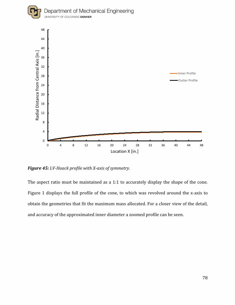
78

Figure 45: LV-Haack profile with X-axis of symmetry.

The aspect ratio must be maintained as a 1:1 to accurately display the shape of the cone.

Figure 1 displays the full profile of the cone, to which was revolved around the x-axis to

obtain the geometries that fit the maximum mass allocated. For a closer view of the detail,

and accuracy of the approximated inner diameter a zoomed profile can be seen.

0

4

8

12

16

20

24

28

32

36

40

44

48

0 4 8 12 16 20 24 28 32 36 40 44 48

Rad

ial D

ista

nce

fro

m C

entr

al A

xis

[in

.]

Location X [in.]

Inner Profile

Outter Profile

79

Figure 46: Zoomed View of the LV-Haack profile with X-axis of symmetry.

The forward end of the nose cone resulted in the most amount of error. The error in

constant thickness tends to zero as x approaches the length of the rocket.

Figure 47: List of mass property results of LV-Haack nose cone as solved by SolidWorks.

0

3

6

9

12

0 3 6 9 12

Rad

ial D

ista

nce

fro

m C

entr

al A

xis

[in

.]

Location X [in.]

Outter Profile

Inner Profile

80

The results shown in figure (47) were calculated by SolidWorks Mass Properties tool.

These results can be compared to the value obtained using the MATLAB procedure

programmed.

Figure 48: Resulting volume of LV-Haack nose cone as solved by program.

The results in figure (47) compare closely to the calculated results shown in figure (48)

using the method described in Materials and Methods section. The mass properties were

compared to SolidWorks models built using the same guessed parameters. The results

calculated were less than 1% difference with respect to the values displayed by the

SolidWorks measurements tool.

Discussion of Program The mass properties for the shell and fin sections of the rocket can be treated as exact

calculations since those geometries are well known. As for the LV-Haack profile, these

calculations are only approximate within 1% accuracy due to their complexity. The error

towards the forward end of the nose cone could be result of calculating the positive root of

the polynomial fit used to define inside of the shape. MATLAB’s fzero command was used to

solve for the polynomial’s root, using a guess of 0.02 [in.] along the length of the nose cone.

The fzero routine iterates until a stop condition was met, for this case, an error less than 10

millionths. Once the root was solved, an array was created using this offset value as the first

index of x.

81

The design method is tentative and has since changed since the start of the project. Initially

the program was first calibrated in order to test the accuracy of calculations. Once the

calculations are properly calibrated, the design architecture and functionality will be

implemented. The program does have a goal, which is to match a cross-sectional area of the

base of the nose cone to the area in the stress calculation along with a clever safety factor.

Pressure Transducer An analog pressure transducer will be used to measure the change of pressure over a

change in time. This data will be used to optimize the amount of black powder charge that

will be used to eject the nose cone and initiate recovery. To do so, a 1600 [psi] pressure

transducer was used. The device is an analog ratiometric sensor with a 5 [Vdc] input with a

max output of 4.5 [Vdc]. The sensor divides the maximum specified rating of 1600 [psi] into

a 10-bit resolution. The sensor will be powered by an Arduino UNO Rev3 microcontroller

and an analog pin will read the signal wire. To obtain the gage pressure the sensor detects,

the bits read from the signal wire will be multiplied by a conversion factor with units of

[psi/bit]. Refer to Arduino code in the appendix for the conversion method.

When the device is first running and ready to collect data the program takes the

average pressure reading over the first half second of being activated. The average pressure

that is obtained and calculated will act as a way to zero the device to read a gage pressure.

The frequency of the data collection is approximately 1000 [Hz]. The results will be printed

to the serial monitor which can then be imported into MATLAB and converted into an array.

Discussion of Code The devices maximum specification of 1600 [psi] too high since it is a ratiometric

device and will be incremented by 10-bits regardless of the voltage input. The pressure step

82

is 2.0 [psi] rounding to the nearest tenth which is too coarse for the data desired. To achieve

better resolution a lower specification is of interest.

Conclusion Having the opportunity to launch a rocket at BALLS 28 was a huge accomplishment

for us. It allowed us to nail down our design and test our skills of mixing a large motor. We

modified the things that we wanted to change and worked towards our goal of building a

large rocket for a high-altitude attempt, but then had to change the design due to budgetary

restrictions. We modified and made a new propellant, changed the design for the forward

closure/adapter to the nose cone, and did more analysis on every part we made either

through flow simulation, finite element analysis, or hand calculations. We are excited for the

day that we get to launch this rocket.

83

References [1] Sutton, George P. , Biblarz, Oscar: Rocket Propulsion Elements : an introduction to the

engineering of rockets. New York: John Wiley & Sons, Inc., 7th ed. 2001. Print.

[2] Boiffier, Jean-Luc. The Dynamics of Flight : The Equations. New York: John Wiley &

Sons, Inc., 1998. Print.

[3] Parker Hannifin Corporation. Parker O-Ring Handbook ORD 5700. 2018. CH 4. Web.

84

Appendices Rocket Basic Sim MATLAB Code

%Rocket_Basic_sim1

clc

clear

close all % Constants

dt=.01;% [s] time step

m0=11.61;% [kg] Initial total mass of rocket

mp=2.992;% [kg] Mass of Propellent

tp=4.4;% [sec] Burn time

Dia=.102;%[m] Max diameter of rocket body

Ar=pi()/4*Dia^2;% [m^2]Ref. Area

YL=1642.68;% [m] Local Altitude

TL=28.7;% [C] Local Temp

RailLength=6.5;%[m]6.5

g=9.81;%[m/s^2]

ta=28.68;%Time to apogee from flight data (Approx)

psi0=86*pi()/180;% [radians] Initial Flight direction from horizontal maxit=1000000;%maximum Iterations

% Preallocate Arrays

dat = zeros(17,maxit); Stat=zeros(15,1); Err=zeros(3,1); Boostexport=zeros(1,6); %Initialize Variables

m=m0; z1=0;z2=0;%Initial Pos X,Y

z3=0;z4=0;%Initial Velocities X,Y

Ay=0;Ax=0;%Initial Accel X,Y

Cd=0; Fd=0; Mprev=0; for i=1:maxit

tt=(i-1)*dt; A=(Ax^2+Ay^2)^(1/2);

85

V=(z3^2+z4^2)^(1/2); Yr=z2;% Hieght of Rocket

%Standard Atmosphere Calc with Offset

[M,Row,P,T,Y]=Atmosphere(YL,Yr,TL,V); [Cd]=Drag_Forensic1(M);%Dragconst; k=Cd/2*Row*Ar; [Ft]=m14002(tt);% Thrust Curve of Motor

%2nd Law Euler Integration

% Rocket Dwells on the lauchpad

if Ay<=0 & tt<tp & z2/sin(psi0)<=RailLength

Ff=.6*cos(psi0)*m*g;%Rail friction

Ax=1/m*(Ft*cos(psi0)-cos(psi0)*Ff); Ay=1/m*(Ft*sin(psi0)-m*g-sin(psi0)*Ff); z1=0; z2=0; z3=0; z4=0; Theta=psi0*180/(pi()); %Rocket launches on rail elseif Ay>=0 & z2/sin(psi0)<=RailLength & tt<tp

Ff=.2*cos(psi0)*m*g; Ay=1/m*(Ft*sin(psi0)-k*V^2*sin(psi0)-m*g-sin(psi0)*Ff); Ax=Ay/tan(psi0); z1=z1+(dt*z3); z2=z2+(dt*z4); z3=z3+dt*Ax; z4=z4+dt*Ay; Theta=psi0*180/(pi()); else% Rocket off the rail Ax=1/m*(Ft*z3/(z3^2+z4^2)^(1/2)-k*abs((z3^2+z4^2)^(1/2))*z3); Ay=1/m*(Ft*z4/(z3^2+z4^2)^(1/2)-k*abs((z3^2+z4^2)^(1/2))*z4-m*g); z1=z1+(dt*z3); z2=z2+(dt*z4);

86

z3=z3+dt*Ax; z4=z4+dt*Ay; Theta=atan2(z4,z3)*180/(pi()); Fd=((k*abs((z3^2+z4^2)^(1/2))*z3)^2+(k*abs((z3^2+z4^2)^(1/2))... *z4)^2)^(1/2); end

%debug

% dat=dat(1:13,1:(i-1));%Truncates data matrix for plotting

% break;end [m]=Mass(mp,tp,m0,tt);% Mass Function for Solid Prop. %Store Data

dat(1,i)=tt;%time

dat(2,i)=z1;%x pos

dat(3,i)=z2;%y pos

dat(4,i)=z3;%x vel dat(5,i)=z4;%y vel dat(6,i)=Ax;%x accel dat(7,i)=Ay;%y accel dat(8,i)=V;% resultant vel

dat(9,i)=A;% resultant accel dat(10,i)=Y;% Altitude

dat(11,i)=M;% Mach#

dat(12,i)=Theta;%[Degrees] Flight Angle

dat(13,i)=m;% mass

dat(14,i)=Yr;% hieght

dat(15,i)=Fd;% Drag Force

dat(16,i)=Ft;% Thrust Force

dat(17,i)=Cd;% Coefficient of Drag

%Drag vs Mach Data Plot

if M>=Mprev

DragForce(1,i)=dat(11,i); DragForce(2,i)=dat(15,i); Dcoeff(1,i)=dat(11,i); Dcoeff(2,i)=dat(17,i);

87

Mprev=M; end %Stores selected Data at the end of burn [T,Yacc,ht,Vres,Ares,Theata]

if tt<=tp

Boost=[dat(:,i)]; Boosttrans=Boost.'; Boostexport=[Boosttrans(1,1) Boosttrans(1,7) Boosttrans(1,14)... Boosttrans(1,8) Boosttrans(1,9) Boosttrans(1,12)]; end

%exports Data for schedules

if tt==ta dattrans=dat(1:17,1:i).'; datexport=[dattrans(:,1) dattrans(:,7) dattrans(:,3) ... dattrans(:,8) dattrans(:,12)]; xlswrite('Sim_Export', datexport); end

%Rocket hits the ground

if z2<=0 & tt>tp

dat=dat(1:17,1:i);%Truncates data matrix for plotting

break

end

end

%Exports Cd Data

Dcoefftrans=[Dcoeff(1,:);Dcoeff(2,:)].'; xlswrite('CD_Export', Dcoefftrans); % max flight statistics [alt(m);speed(m/s);accel(m/s^2);Mach#]

FlightStat=[6607.48;445.3;165.4;1.3]; Stat= max(dat,[],2);% Retrieves max values of each row in the dat[]

MaxAccRes=Stat(9,1); %Max Acceleration along rocket axis

[I,J] = find(dat== MaxAccRes);% Finds the subscript

MaxAccResDat=dat(:,J);% Column vector of data for max resultant accel %Calculate Error Percentage

Err=[abs(FlightStat(1,1)-Stat(10,1))/FlightStat(1,1)*100;%altitude

abs(FlightStat(2,1)-Stat(8,1))/FlightStat(2,1)*100;%speed

abs(FlightStat(3,1)-Stat(7,1))/FlightStat(3,1)*100;%vert accel

88

abs(FlightStat(4,1)-Stat(11,1))/FlightStat(4,1)*100];%Mach #

fprintf('Altitude\n'); fprintf( 'Flight %3.1f m\t',FlightStat(1,1)); fprintf( 'Calculated %3.1f m\t',Stat(10,1)); fprintf( 'Percentage Error %3.1f \n',Err(1,1)); fprintf('Speed\n'); fprintf( 'Flight %3.1f m/s\t',FlightStat(2,1)); fprintf( 'Calculated %3.1f m/s\t',Stat(8,1)); fprintf( 'Percentage Error %3.1f\n',Err(2,1)); fprintf('Vertical Acceleration\n'); fprintf( 'Flight %3.1f m/s^2\t',FlightStat(3,1)); fprintf( 'Calculated %3.1f m/s^2\t',Stat(7,1)); fprintf( 'Percentage Error %3.1f\n',Err(3,1)); fprintf('Mach #\n'); fprintf( 'Flight %3.1f m/s^2\t',FlightStat(4,1)); fprintf( 'Calculated %3.1f m/s^2\t',Stat(11,1)); fprintf( 'Percentage Error %3.1f\n',Err(4,1)); figure(1)

plot(dat(1,:),dat(4,:),dat(1,:),dat(5,:))

title('Velocities')

xlabel('Time [s]')

ylabel('Velocity[m/s]')

legend('X','Y')

figure(2)

plot(dat(2,:),dat(3,:))

title('Trajectory')

xlabel('Distance[m]')

ylabel('Height[m]')

figure(3)

plot(dat(1,:),dat(8,:))

title('Velocity')

xlabel('Time [s]')

ylabel('Velocity[m/s]')

figure(4)

plot(dat(1,:),dat(7,:))

89

title('Vertical Acceleration')

xlabel('Time [s]')

ylabel('Acceleration[m/s^2]')

figure(5)

plot(dat(1,:),dat(10,:))

title('Altitude vs Time')

xlabel('Time [s]')

ylabel('Altitude[m]')

figure(6)

plot(DragForce(1,:),DragForce(2,:))

title('Drag Force vs Mach #')

xlabel('Mach #')

ylabel('Drag Force [N]')

figure(7)

plot(dat(1,:),dat(14,:))

title('Verical Displacement vs Time')

xlabel('Time [s]')

ylabel('Hieght[m]')

figure(8)

plot(Dcoeff(1,:),Dcoeff(2,:))

title('Cd vs Mach #')

xlabel('Mach #')

ylabel('Cd')

%Coast_sim1

clc

clear

close all % Constants

dt=.01;% [s] time step

Dia=.102;%[m] Max diameter of rocket body

Ar=pi()/4*Dia^2;% [m^2]Ref. Area

YL=1642.68;% [m] Local Altitude

TL=28.7;% [C] Local Temp

g=9.81;%[m/s^2]

maxit=1000000;%maximum Iterations

% Preallocate Arrays

90

dat = zeros(17,maxit); Stat=zeros(15,1); Err=zeros(3,1); Boostexport=zeros(1,6); %Export from Coast Data Initial conditions

maxt=24.28; Vr=434.74; tilt=5.53; Ayr=0; ht=1367.92; %Initialize Variables

m=8.618;%Mass empty

psi0=(90-tilt)*pi()/180;% [radians] Initial Flight direction from horizontal z1=ht*atan(psi0);z2=ht;%Initial Pos X,Y

z3=Vr*cos(psi0);z4=Vr*sin(psi0);%Initial Velocities X,Y

Ay=0;Ax=0;%Initial Accel X,Y

Cd=0; Fd=0; Ft=0; Mprev=0; for i=1:maxit

tt=(i-1)*dt; A=(Ax^2+Ay^2)^(1/2); V=(z3^2+z4^2)^(1/2); Yr=z2;% Hieght of Rocket

[M,Row,P,T,Y]=Atmosphere(YL,Yr,TL,V);%Standard Atmosphere Calc with Offset [Cd]=Drag_Forensic1(M); k=Cd/2*Row*Ar; % Rocket off the rail Ax=1/m*(Ft*z3/(z3^2+z4^2)^(1/2)-k*abs((z3^2+z4^2)^(1/2))*z3); Ay=1/m*(Ft*z4/(z3^2+z4^2)^(1/2)-k*abs((z3^2+z4^2)^(1/2))*z4-m*g);

91

z1=z1+(dt*z3); z2=z2+(dt*z4); z3=z3+dt*Ax; z4=z4+dt*Ay; Theta=atan2(z4,z3)*180/(pi()); Fd=((k*abs((z3^2+z4^2)^(1/2))*z3)^2+... (k*abs((z3^2+z4^2)^(1/2))*z4)^2)^(1/2);

%Store Data

dat(1,i)=tt;%time

dat(2,i)=z1;%x pos

dat(3,i)=z2;%y pos

dat(4,i)=z3;%x vel dat(5,i)=z4;%y vel dat(6,i)=Ax;%x accel dat(7,i)=Ay;%y accel dat(8,i)=V;% resultant vel

dat(9,i)=A;% resultant accel dat(10,i)=Y;% Altitude

dat(11,i)=M;% Mach#

dat(12,i)=Theta;%[Degrees] Flight Angle

dat(13,i)=m;% mass

dat(14,i)=Yr;% hieght

dat(15,i)=Fd;% Drag Force

dat(16,i)=Ft;% Thrust Force

dat(17,i)=Cd;% Coefficient of Drag

%Drag vs Mach Data Plot

if M>=Mprev

DragForce(1,i)=dat(11,i); DragForce(2,i)=dat(15,i); Dcoeff(1,i)=dat(11,i); Dcoeff(2,i)=dat(17,i); Mprev=M; end

%exports Data for schedules

if tt==maxt dattrans=dat(1:17,1:i).';

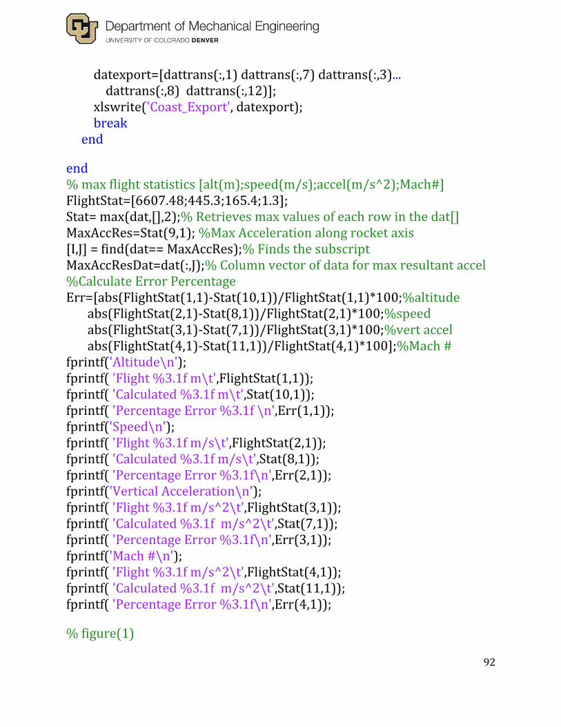
92

datexport=[dattrans(:,1) dattrans(:,7) dattrans(:,3)... dattrans(:,8) dattrans(:,12)]; xlswrite('Coast_Export', datexport); break

end end

% max flight statistics [alt(m);speed(m/s);accel(m/s^2);Mach#]

FlightStat=[6607.48;445.3;165.4;1.3]; Stat= max(dat,[],2);% Retrieves max values of each row in the dat[]

MaxAccRes=Stat(9,1); %Max Acceleration along rocket axis

[I,J] = find(dat== MaxAccRes);% Finds the subscript

MaxAccResDat=dat(:,J);% Column vector of data for max resultant accel %Calculate Error Percentage

Err=[abs(FlightStat(1,1)-Stat(10,1))/FlightStat(1,1)*100;%altitude

abs(FlightStat(2,1)-Stat(8,1))/FlightStat(2,1)*100;%speed

abs(FlightStat(3,1)-Stat(7,1))/FlightStat(3,1)*100;%vert accel abs(FlightStat(4,1)-Stat(11,1))/FlightStat(4,1)*100];%Mach #

fprintf('Altitude\n'); fprintf( 'Flight %3.1f m\t',FlightStat(1,1)); fprintf( 'Calculated %3.1f m\t',Stat(10,1)); fprintf( 'Percentage Error %3.1f \n',Err(1,1)); fprintf('Speed\n'); fprintf( 'Flight %3.1f m/s\t',FlightStat(2,1)); fprintf( 'Calculated %3.1f m/s\t',Stat(8,1)); fprintf( 'Percentage Error %3.1f\n',Err(2,1)); fprintf('Vertical Acceleration\n'); fprintf( 'Flight %3.1f m/s^2\t',FlightStat(3,1)); fprintf( 'Calculated %3.1f m/s^2\t',Stat(7,1)); fprintf( 'Percentage Error %3.1f\n',Err(3,1)); fprintf('Mach #\n'); fprintf( 'Flight %3.1f m/s^2\t',FlightStat(4,1)); fprintf( 'Calculated %3.1f m/s^2\t',Stat(11,1)); fprintf( 'Percentage Error %3.1f\n',Err(4,1)); % figure(1)

93

% plot(dat(1,:),dat(4,:),dat(1,:),dat(5,:))

% title('Velocities')

% xlabel('Time [s]')

% ylabel('Velocity[m/s]')

% legend('X','Y')

% figure(2)

% plot(dat(2,:),dat(3,:))

% title('Trajectory')

% xlabel('Distance[m]')

% ylabel('Height[m]')

% figure(3)

% plot(dat(1,:),dat(8,:))

% title('Velocity')

% xlabel('Time [s]')

% ylabel('Velocity[m/s]')

% figure(4)

% plot(dat(1,:),dat(7,:))

% title('Vertical Acceleration')

% xlabel('Time [s]')

% ylabel('Acceleration[m/s^2]')

% figure(5)

% plot(dat(1,:),dat(10,:))

% title('Altitude vs Time')

% xlabel('Time [s]')

% ylabel('Altitude[m]')

% figure(6)

% plot(DragForce(1,:),DragForce(2,:))

% title('Drag Force vs Mach #')

% xlabel('Mach #')

% ylabel('Drag Force [N]')

% figure(7)

% plot(dat(1,:),dat(14,:))

% title('Verical Displacement vs Time')

% xlabel('Time [s]')

% ylabel('Hieght[m]')

94

%Drag_Forensic1

function[Cd]=Drag_Forensic1(M)

fudge=0.09; Cons=.8; if M<=Cons

M=Cons; Cd=-19.241*M^3+56.037*M^2-52.769*M+16.561+fudge; %Cd=1.8433*M^3-0.1717*M^2+.0356*M;

elseif M>Cons & M<=1.2

Cd=-19.241*M^3+56.037*M^2-52.769*M+16.561+fudge; else

Cd=-M+1.9736; End %m14002

function[Ft]=m14002(tt)% average thrust peak

if tt>=0 & tt<.02

Ft=49581*tt; elseif tt>=.02 & tt<.07

Ft=18961*tt+612.39; elseif tt>=.07 & tt<.11

Ft=4363.5*tt+1634.2; elseif tt>=.11 & tt<.14

Ft=-4593.7*tt+2619.5; elseif tt>=.14 & tt<3.53

Ft=-11.045*tt^2-182.34*tt+1988.6; elseif tt>=3.53 & tt<3.7

Ft=-14822*tt^2+105456*tt-186364; elseif tt>=3.7 & tt<4.43

Ft=604.45*tt^2-5948.2*tt+14638; else

Ft=0; end

95

Ft=.97*Ft; End %Atmosphere

function[M,Row,P,T,Y]=Atmosphere(YL,Yr,TL,V)

K=1.4;% Ratio of spec. heat AIR

R=287; %[J/kg*K] Gas constant

tL=TL+273.1; % [K] local temperature

Y=YL+Yr;%[m] Altitude

alpha=-0.00357/(1.8*0.3048);%[change in K or Cels. per meter]

P0=101300;% [Pa]

T0=tL-alpha*YL; Row=P0/R*((T0+alpha*Y)^(4.26))/(T0^(5.26));% density {kg/m^3]

P=P0*((T0+alpha*Y)/T0)^(5.26);%[pa] Pressure at Altitude

T=P/(Row*R);%[K] Temp at Altitude

M=V/((K*R*T)^(1/2)); %Mach Number

end

Distributed Mass Properties Program

%Program by Kian Roybal

%Date Created Friday, Sept 20, 2019

%Date Modified Tuesday, October 8, 2019

%Description:

%This program will assist in the design process by allowing a stream-lined

%way to distribute an allowed mass through the distinct sections of the

%rocket. Given a governing diameter is known, and an output

%maximum-allowed-mass from the properties and kinetics calculator are known

%this routine will solve for the thickness that meets it to a safety factor

%stress such that the cross-sectional area satisfies this criteria.

%

%*NOTE* the design method is tentative and is subject to change. Currently

%a change is undergoing, and this file up-to-date does NOT meet the

%description but soon to be updated to function as such.

%Initiate:

clc;clear;close all

%===========================%

%===== Rocket sections =====%

96

%===========================%

%==Material properties===%

%-- Density of material [lb/in.^3]

rho_Al = 0.1;

rho_fiber = .05;

%Governing dimension:

%-- Diameter

D = 8; %[in.]

R = D/2; %[in.]

%-- Motor tube [in.]

D_tube = 4;

%this parameter describes the length in which the tube extends from aft end

tube_extended = 4;

L_tube = 12*5+tube_extended;

th_tube = 0.25;

ID_tube = D_tube-th_tube;

[xbar_tube, ybar_tube, zbar_tube, m_tube] = ...

shell_masscenter(ID_tube,D_tube,L_tube,rho_Al);

Z_cbar_tube = zbar_tube;

%-- Aft end [in.]

L_aft = 12*5;

th_aft = 0.25;

ID_aft = D-th_aft;

[xbar_aft, ybar_aft, zbar_aft, m_aft] = shell_masscenter(ID_aft,D,...

L_aft,rho_Al);

Z_cbar_aft = zbar_tube+tube_extended;

%-- Center/Ebay [in.]

L_ebay = 12*1;

th_ebay = 0.25;

ID_ebay = D-th_ebay;

[xbar_ebay, ybar_ebay, zbar_ebay, m_ebay] = ...

shell_masscenter(ID_ebay,D,L_ebay,rho_fiber);

Z_cbar_ebay = Z_cbar_aft+zbar_ebay;

%-- Nosecone [in.]

L_nose = 48;

th_nose = 0.5;

[m_nose,zbar_nose,lala,lsdf,V] = LVH_masscenter(D,th_nose,L_nose,rho_Al);

Z_cbar_nose = Z_cbar_ebay+zbar_nose;

%-- Fincan [in]

L_fincan = 10;

th_fincan = 0.125;

D_fincan = D+th_fincan;

[xbar_fincan, ybar_fincan, zbar_fincan, m_fincan] = ...

97

shell_masscenter(D,D_fincan,L_fincan,rho_Al);

Z_cbar_fincan = Z_cbar_tube + zbar_fincan;

%Fins

th_fin = 0.125;

%This parameter describes distance the point closest to aft end

fins_extended = 2;

%Fin Root Chord

Cr = 8;

%Fin Tip Chord

Ct = 7;

%Fin Semispan

S = 6;

%Midpoint length

Lf = 10.5;

%unitary fin data

[xbar_fin, ybar_fin, zbar_fin, m_fin] = ...

fin_masscenter(Cr, Ct, S, Lf, th_fin, rho_Al);

%Z_cbar_fins = Z_cbar_tube+fins_extended+zbar;

%Misc. units

n_fins = 4;

theta_seperation = 360/n_fins; %[deg.]

m_fins = m_fin*n_fins;%[lb]

%ZBAR = sum(Z_cbar_i*vol_i)/sum(vol_i);

%Total mass

mass = [m_aft,m_fincan,m_fins,m_tube,m_ebay,m_nose];

mass_Total = sum(mass);%[lb]

V = V*(2.54e1)^3;

fprintf('Resulting Volume of the LV-Haack nosecone is: %1.3e [mm^3]',V);

Code Block 1: Main Routine

function [mass,zbar,outter,inner,vol] = LVH_masscenter(D,th,L,rho)

num = 400;

dx = L/num;

R = D/2;

syms x u

func_radicand = acos(1-2*x/L)-sin(2*acos(1-2*x/L))/2+...

(2/3)*sin(acos(1-2*x/L))^3;

func = R/sqrt(pi)*sqrt(func_radicand);

OD_int = pi*int(func^2,x,0,L);

98

dfunc = diff(func);

dfunc = matlabFunction(dfunc);

func = matlabFunction(func);

len = length(0:dx:L);

[Y,X] = deal(zeros(1,len));

[xx,yy] = deal(zeros(1,len-1));

N = zeros(2,len-1);

for i = 1:len

X(i) = (i-1)*dx;

Y(i) = func(X(i));

if i > 1

Ni = [dfunc(X(i));-1];

Nj = th*Ni/norm(Ni);

N (:,i-1) = Nj;

xx(i-1) = X(i)+Nj(1,1);

yy(i-1) = Y(i)+Nj(2,1);

end

end

%The First least squares fit will be used to solve for the function that

%defines thes the inside radius of the nosecone

%=========================

%----- LEAST SQUARES -----

%--- Sixth order model ---

%=========================

A = ones(len-2,7); flex = xx';

A(:,6) = flex(1:end-1);

bb = yy'; b = bb(1:end-1);

for k = 1:1:len-2

A(k,1) = xx(k)^6; A(k,2) = xx(k)^5; A(k,3) = xx(k)^4;

A(k,4) = xx(k)^3; A(k,5) = xx(k)^2;

end

v = (A'*A)\A'*b;

clc;

func_6th = @(xx) v(1)*xx^6+v(2)*xx^5+v(3)*xx^4+v(4)*xx^3+v(5)*xx^2+...

v(6)*xx+v(7);

xroot = fzero(func_6th,.1,optimset('TolX',1e-8,'Display','off'));

dxx = (L-xroot)/(num-1);

xarray = xroot:dxx:L;

yarray = zeros(1,num);

for i = 1:1:num

yarray(i) = func_6th(xarray(i));

end

%LV-HAACK function inserted into the mass center definition

%was not integrable by matlab fit the points and integrate the 7th order

%Polynomial fit

99

%=========================

%----- LEAST SQUARES -----

%-- Seventh order model --

%=========================

A = ones(len,8); flex_2 = X';

A(:,7) = flex_2;

jj = Y';

for k = 1:1:len

A(k,1) = X(k)^7; A(k,2) = X(k)^6; A(k,3) = X(k)^5;

A(k,4) = X(k)^4; A(k,5) = X(k)^3; A(k,6) = X(k)^2;

end

vv = (A'*A)\A'*jj;

func_7th = @(xx) vv(1)*xx^7+vv(2)*xx^6+vv(3)*xx^5+vv(4)*xx^4+vv(5)*xx^3+...

vv(6)*xx^2+vv(7)*xx+vv(8);

xroot2 = fzero(func_7th,.1,optimset('TolX',1e-8,'Display','off'));

dxx2 = (L-xroot2)/(num);

xarray2 = xroot2:dxx2:L;

yarray2 = zeros(1,num);

for i = 1:1:len

yarray2(i) = func_7th(xarray2(i));

end

OD_fn = vv(1)*u^7+vv(2)*u^6+vv(3)*u^5+vv(4)*u^4+vv(5)*u^3+...

vv(6)*u^2+vv(7)*u+vv(8);

OD_Myz = int(u*OD_fn,u,xroot2,L);

OD_mm = int(OD_fn,u,xroot2,L);

ID_fn = v(1)*u^6+v(2)*u^5+v(3)*u^4+v(4)*u^3+v(5)*u^2+...

v(6)*u+v(7);

ID_int = pi*int(ID_fn^2,u,xroot,L);

ID_Myz = int(u*ID_fn,u,xroot,L);

ID_mm = int(ID_fn,u,xroot,L);

zbar = double((OD_Myz-ID_Myz)/(OD_mm-ID_mm));

zbar = L - zbar;

vol = double(OD_int - ID_int);

mass = rho*vol;

clc;

outter = [X' Y'];

inner = [xarray' yarray'];

end

Code Block 2: LV-Haack Routine

function [xbar, ybar, zbar, m] = fin_masscenter(Cr, Ct, S, Lf, Th, rho)

%DESCRIPTION:

%This function file will return 3D mass center coordinates of a singular

%fin, as well as its mass

%

100

%----- output is formatted as follows:

%----- [xbar, ybar, zbar, mass]

%----- Input index:

%----- 1) Cr = Fin Root Chord :::: dimension: [L]

%----- 2) Ct = Fin Tip Chord :::: dimension: [L]

%----- 3) S = Fin Semispan :::: dimension: [L]

%----- 4) Lf = Midpoint length :::: dimension: [L]

%----- 5) Th = Thickness :::: dimension: [L]

%----- 6) rho = desnity :::: dimension: [M/L^3]

%=========================================================================

%Calculated geometry

del = sqrt(Lf^2 - S^2);

l1 = Cr/2 + del - Ct/2;

l2 = Cr/2 + del + Ct/2;

%Composite shape made up of 2 right triangles and a rectangle

%--- Index: [1] Triangle [2] Rectangle [3] Triangle

A1 = 1/2*l1*S;

V1 = A1*Th;

m1 = V1*rho;

xbar1 = 1/3*S;

ybar1 = 2/3*l1;

A2 = (Cr-l1)*S;

V2 = A2*Th;

m2 = V2*rho;

xbar2 = 1/2*S;

ybar2 = l1+1/2*(Cr-l1);

A3 = 1/2*(l2-Cr)*S;

V3 = A3*Th;

m3 = V3*rho;

xbar3 = 2/3*S;

ybar3 = Cr + (1/3)*(l2-Cr);

m = m1 + m2 + m3;

%Compute mass center

xbar = (xbar1*m1 + xbar2*m2 + xbar3*m3)/m;

ybar = (ybar1*m1 + ybar2*m2 + ybar3*m3)/m;

zbar = 0;

end

Code Block 3: Fin Mass Routine

function [xbar, ybar, zbar, m, V] = shell_masscenter(ID, OD, h, rho)

%DESCRIPTION:

101

%This function file will return 3D mass center coordinates of a singular

%shell (tube section), as well as its mass.

%

% IMPORTANT NOTE:

% ----- [ for solid cylinder take ID input = 0 ] ----

%

%note: datum of shell is the aft end, with cardinal axes through center

%

%----- output is formatted as follows:

%----- [xbar, ybar, zbar, mass]

%----- Input index:

%----- 1) ID = inner diameter :::: dimension: [L]

%----- 2) OD = outter diameter :::: dimension: [L]

%----- 3) h = height of shell :::: dimension: [L]

%----- 4) rho = desnity :::: dimension: [M/L^3]

%=========================================================================

%Calculate cross sectional area:

A = pi*1/4*(OD^2 - ID^2);

%Calculate mass properties

V = A*h;

m = V*rho;

%by symmetry and orientation xbar and zbar are centered on origin

xbar = 0;

ybar = 1/2 * h;

zbar = 0;

end

Code Block 4: Shell Mass Routine

Arduino Pressure Transducer Code

/*Author: Kian C Roybal

*

* Description:

* Analog read, the output of a pressure transducer. The pressure transducer is a

ratiometric,

* from 10% to 90% of the power supply voltate. Therefore the analoRead on the pin

should give

* an output that is also a ratio against the maximum specifcation of 1600psi

*

102

*/

//Pin number 14 is the A0 for the arduino uno r3

int dataPin = 14;

//Analog read value corresponding to the reading of the transducer

int val = 0;

int atmospheric = 0;

float atm = 0.0;

float maxPSI = 1600.0;

float maxval = 921.0;

float max1600;

float readPSI;

float gagePressure;

void setup() {

//Initialize the baud rate of 9600

Serial.begin(9600);

//Begin zeroing atmospheric pressure

delay(100);

atmospheric = analogRead(dataPin);

atm = atmospheric;

delay(100);

atmospheric = analogRead(dataPin);

atm = atm + atmospheric;

delay(100);

atmospheric = analogRead(dataPin);

103

atm = atm + atmospheric;

delay(100);

atmospheric = analogRead(dataPin);

atm = atm + atmospheric;

delay(100);

atmospheric = analogRead(dataPin);

atm = atm + atmospheric;

atm = int(atm/5);

//Atmospheric zeroing complete

Serial.println("Atmospheric rating: ");

Serial.print(atm);

Serial.println("");

delay(1000);

}

void loop() {

val = analogRead(dataPin);

//offset the atmospheric reading to act as a zero

max1600 = maxval - atm;

readPSI = val - atm;

//zeroing complete

//converts the bits to a gagepressure

gagePressure = maxPSI *readPSI/max1600;

//Print data

104

Serial.println("byte reading: ");

Serial.print(val);

Serial.println("");

Serial.println("Pressure reading: ");

Serial.print(gagePressure);

Serial.print(" [psi]");

Serial.println("");

Serial.println("");

delay(1);//1000 data per second

}

[End of Arduino code: Pressure Transducer]