MA 151, Applied Calculus, Fall 2017, Final Exam Preview 1...

MA 151, Applied Calculus, Fall 2017, Final Exam Preview 1

Basic Functions

1. Identify each of the graphs below as one of the following functions:

x3 − 4x2 + x

ex

ln(x)

x2

x3

(1/2)x

2

−x4 + 4x2 + 10

5x− 10

−5x+ 10

Function notation, solving function equations

2. (This problem as a whole is obviously too long for the final: but I could have a problem with a coupleof parts like this.)

(a) Let f(x) = 3x+ 5. Solve f(x) = 3.

Solution:

3x+ 5 = 3

3x = −2x = −2/3

(b) Let f(x) = x2. Solve f(x) = 5.

Solution:

x2 = 5

x = ±√5


(c) Let f(x) = 2x3 − 5. Solve f(x) = −10.

Solution:

2x3 − 5 = −102x3 = −5

x3 = −5

3

x =3

√−5

3

= − 3√5/3

(d) Let f(x) = x2 − 2x− 15. Solve f(x) = 0.

Solution:

x2 − 2x− 15 = 0

(x− 5)(x+ 3) = 0

(x− 5) = 0 or (x+ 3) = 0

x = 5 or − 3

(e) Let f(x) = x2 − 2x− 14. Solve f(x) = 0.

Solution:

x2 − 2x− 14 = 0

x =2±

√(−2)2 − 4(1)(−14)

2(1)

=2±√4 + 56

2

=2±√60

2

(f) Let f(x) = ex − 2x2ex. Solve f(x) = 0.

Solution:

ex − 2x2ex = 0

ex(1− 2x2) = 0

ex = 0 or (1− 2x2) = 0

ex = 0 is impossible

1− 2x2 = 0

2x2 = 1

x2 = 1/2

x = ±√1/2

4

(g) Let f(x) =1

x+ 1. Solve f(x) = 0.

Solution:

1

x+ 1 = 0

1

x= −1

1

x=−11

1 = −x (cross multiply)

x = −1

(h) Let f(x) =2

x2− 5. Solve f(x) = 0.

Solution:

2

x2− 5 = 0

2

x2= 5

2

x2=

5

1

2 = 5x2 (cross multiply)

x2 = 2/5

x = ±√2/5

(i) Let f(x) = 3ex − 5. Solve f(x) = 0.

Solution:

3ex − 5 = 0

3ex = 5

ex = 5/3

ln(ex) = ln(5/3)

x = ln(5/3)

(j) Let f(x) = 4e2x − 3. Solve f(x) = 0.

Solution:

4e2x − 3 = 0

4e2x = 3

e2x = 3/4

ln(e2x) = ln(3/4)


2x = ln(3/4)

x =1

2ln(3/4)

(k) Let f(x) = ln(x) + 5. Solve f(x) = 0.

Solution:

ln(x) + 5 = 0

ln(x) = −5eln(x) = e−5

x = e−5

(l) Let f(x) = 2 ln(x)− 5. Solve f(x) = 0.

Solution:

2 ln(x)− 5 = 0

2 ln(x) = 5

ln(x) = 5/2

eln(x) = e5/2

x = e5/2

(m) Let f(x) = 3 ln(x+ 1) + 7. Solve f(x) = 0.

Solution:

3 ln(x+ 1) + 7 = 0

3 ln(x+ 1) = −7ln(x+ 1) = −7/3eln(x+1) = e−7/3

(x+ 1) = e−7/3

x = e−7/3 − 1

3. Let f(x) = x2 and g(x) =1

x+ 1.

(a) Find f(x) + g(x).

Solution:

x2 +1

x+ 1.

(b) Find f(x)g(x).

Solution:

x2

(1

x+ 1

).

6

(c) Findf(x)

g(x).

Solution:x2

1x + 1

.

(d) Find f(g(x)).

Solution:

f

(1

x+ 1

)=

(1

x+ 1

)2

.

(e) Find g(f(x)).

Solution:

g(x2) =1

x2+ 1.

Linear, Power Function, and Exponential Modelling

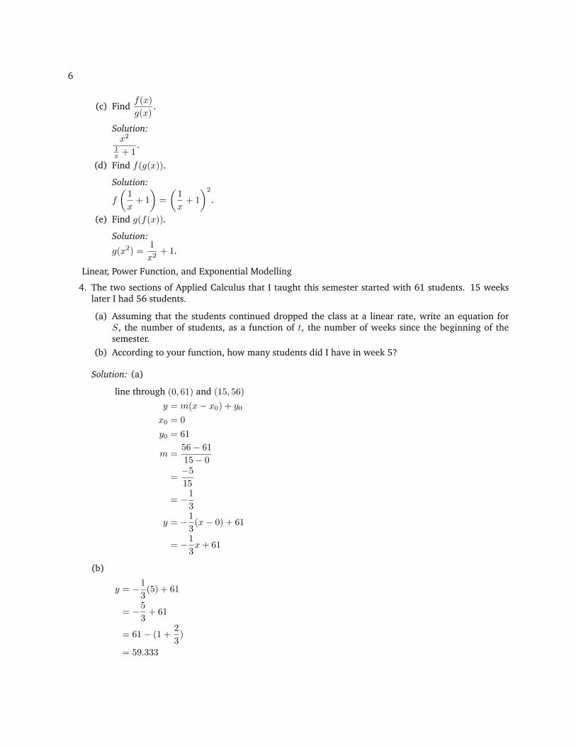
4. The two sections of Applied Calculus that I taught this semester started with 61 students. 15 weekslater I had 56 students.

(a) Assuming that the students continued dropped the class at a linear rate, write an equation forS, the number of students, as a function of t, the number of weeks since the beginning of thesemester.

(b) According to your function, how many students did I have in week 5?

Solution: (a)

line through (0, 61) and (15, 56)

y = m(x− x0) + y0

x0 = 0

y0 = 61

m =56− 61

15− 0

=−515

= −1

3

y = −1

3(x− 0) + 61

= −1

3x+ 61

(b)

y = −1

3(5) + 61

= −5

3+ 61

= 61− (1 +2

3)

= 59.333


5. The arctic ice caps appears to be shrinking at a rate of 4% per decade1.

(a) Assuming that the rate of decrease of ice remains the same, write an equation for I, the percentof the current ice that will be left, as a function of t, the number of decades from now.

(b) According to your equation, what percent of the current amount ice will be left in 50 years?

Solution: (a)

I = Cat C = % of current ice, t=decades, a = 1 + r, r = % change

= 1 · (1− 0.04)t

I = (0.96)t

(b)

I = (0.96)5

= 0.815

= 81.5% of current ice

Functions in Economics

6. (Hughes-Hallet, 4e, #9) A company that makes Adirondack chairs has fixed costs of $5000 and variablecosts of $30 per chair. The company sells the chairs for $50 each.

(a) Find formulas for the cost and revenue functions.

(b) Find the marginal cost and marginal revenue.

(c) Graph the cost and revenue functions on the same axes.

(d) Find the break-even point.

Solution:

(a)

C(q) = 5000 + 30q

R(q) = 50q

(b)

MC = 30

MR50

1From http://www.theguardian.com/environment/2013/sep/18/how-fast-is-arctic-sea-ice-melting

8

(c)

(d)

C(q) = R(q)

5000 + 30q = 50q

20q = 5000

q =5000

20q = 250

7. (Hughes-Hallett, 4e, #28) The demand curve for a product is given by q = 120, 000 − 500p and thesupply curve is given by q = 1000p for 0 ≤ q ≤ 120, 000, where price is in dollars.

(a) At a price of $100, what quantity are consumers willing to buy and what quantity are producerswilling to supply? Will the market push prices up or down?

(b) Find the equilibrium price of quantity. Does your answer to part (a) support the observation thatmarket forces tend to push prices closer to the equilibrium price?

Solution:

(a)

consumers willing to buy: q120, 000− 500p

= 120, 000− 500(100)

= 70, 000

suppliers willing to make: q = 1000p

= 1000(100)

= 100, 000

Market forces will move prices down, because there are too many items being made.

(b)

supply = demand

1000p = 120000− 500p


500p = 120000

p =120000

500= 80

This agrees with (a) because from p = 100 the price will move down to p = 80.

Approximating the Derivative

8. Let f(x) = e−x2

. Find an approximation of f ′(2) by filling in the following table using the same rulesas on the quiz2.

Solution:

x f(x)f(2)− f(x)

2− x

1.9 0.02705185 −0.087362081.99 0.01906121 −0.074556921.999 0.01838903 −0.073390892 0.01831564 ERR2.1 0.01215518 −0.061604612.01 0.01759571 −0.071992612.001 0.01824250 −0.07313447

The numbers we calculated for x = 1.999 and 2.001 are our best approximations. From them we cansay

f ′(2) ≈ −0.073

Graphing Derivatives

9. Shown below is the graph of a cubic function, i.e. a function of the form y = ax3 + bx2 + cx+d. Sketcha graph of the derivative; make sure that your sketch is positive/negative/zero in the right places, andthat it has the right shape.

Solution:

2You should plug numbers in for x that are close to 2. They should be close enough that you get two approximations of f ′(2) thatare the same to the second decimal place. You should always use at least 8 digits in every step of the calculation.

10

To see how to make the second graph, start with the points where f is flat:

graph of f(x) : m = 0 at x = −1.5 and x = 1.5


This means that the graph of f ′(x) should have

graph of f ′(x) : y = 0 at x = −1.5 and x = 1.5

Similarly, see where f is going up:

graph of f(x) : m ≈ 2 at x = −2 and x = 2


graph of f ′(x) : y = 2 at x = −2 and x = 2

Finally, see where f is going down:

graph of f(x) : m ≈ −3 at x = 0


graph of f ′(x) : y = −3 at x = 0

Marginal Cost and Revenue

10. The graph below shows a total cost function. Estimate the marginal cost at q = 700.

Solution: We start by graphing a tangent line (simply move a straight edge towards the graph of C(q)until it just barely touches the graph at q = 700)

Now we estimate the slope of the straight line. The best way to do this is to use points that are as farapart as possible, or to see if the line intersects exactly at one of the grid points.

I’ll use points far apart:(0, 210) and (1000, 810)

12

appear to be on the line. Thus

MC = m ≈ 810− 210

1000− 0=

600

1000= 3/5

11. A company is making complicated things with a cost function given by C(q) = 7e−q − 5√q + 11000q2

and revenue function given by R(q) = 25000q.

(a) Find the marginal cost and marginal revenue.

(b) At q = 300 is the profit increasing or decreasing?

Solution:

(a)

MC =d

dqC(q)

= −7e−q − 5

2q−1/2 + 22000q

MR =d

dqR(q)

= 25000

(b)

MC(300) = −7e−300 − 5

2(300)−1/2 + 22000(300)

= 6599999.86

MR(300) = 25000

Profic is decreasing since MC > MR.

Basic derivatives

12. Find the following derivatives

(a)d

dx3x6

Solution:18x5

(b)d

dx5 3√x

Solution:5

3x−2/3 (note that 3

√x = x1/3)

(c)d

dx

10

x5

Solution:

−50x−6 (note that10

x5= 10x−5)


(d)d

dx17ex

Solution:17ex

(e)d

dx17 ln(x)

Solution:

17 · 1x

Combinations of functions


(a)d

dx3(2x− 5)6

Solution:

d

dx3(2x− 5

)6

= 18(2x− 5

)5

· 2x− 5′

= 18(2x− 5)5 · 2

(b)d

dx5 3√−7x+ 11

Solution:

d

dx5 3

√−7x+ 11 =

5

3

(−7x+ 11

)−2/3

· −7x+ 11′

=5

3(−7x+ 11)

−2/3 · (−7)

(c)d

dx

10

(4x− 5)5

Solution:

d

dx

10

( 4x− 5 )5= −50

(4x− 5

)−6

· 4x− 5′

= −50 (4x− 5)−6 · 4

(d)d

dx17e−x+10

Solution:

d

dx17e−x+1017e

−x+ 10· −x+ 10

′

17e−x+10

· (−1)

14

(e)d

dx17 ln(3x+ 5)

Solution:

d

dx17 ln

(3x+ 5

)= 17 · 1

3x+ 5· 3x+ 5

′


(a)d

dx(3x6 + 5 3

√x)(

10

x5− 17ex)

Solution:

d

dx(3x6 + 5 3

√x)︸︷︷︸

f

(10

x5− 17ex)︸︷︷︸g

f ′ = 18x5 +5

3x−2/3

g′ = −50x−6 − 17ex

f ′g + fg′ =

(18x5 +

5

3x−2/3

)(10

x5− 17ex

)+ (3x6 + 5 3

√x) ·

(−50x−6 − 17ex

)

(b)d

dx

2x2 − x

ex + x2

2x2 − x

ex + x2

← f

← g

f ′ = 4x− 1

g′ = ex + 2x

f ′g − fg′

g2=

(4x− 1)(ex + x2)− (2x2 − x)(ex + 2x)

(ex + x2)2

Derivatives and Tangent Lines

15. (a) Find the Equation of tangent line at x = 5 for f(x) = ln(x).

Solution:

ym(x− x0) + y0

x0 = 5

y0 = f(5) = ln(5)

f ′(x) =1

x

m = f ′(5) =1

5

y =1

5(x− 5) + ln(5)


(b) Find the Equation of tangent line at x = 9 for f(x) = 5√x.

Solution:

ym(x− x0) + y0

x0 = 9

y0 = f(9) = 5√9

= 15

f ′(x) =5

2x−1/2

m = f ′(9) =5

2(9)−1/2

=5

2· 1√

9

=5

2· 13

=5

6

y =5

6(x− 9) + 15

Local Max/Mins

16. Let f(x) = 3x4 − 4x3.

(a) Using your calculator, graph f(x). Use a window that shows all the “interesting” features (inparticular it should show the local max/mins).

Solution:

Note: your window has to be small enough that I can see two things: (1) that the point at (0, 0)is neither a max nor min, (2) that the point (1,−1) is a local min.

16

(b) Describe the critical points, the local max and mins, and where the function is increasing/decreasing.

Solution:critical points: x = 0, 1x = 1 is l. min at x = 1.x = 0 is neitherf ↑ to right of x = 1.f ↓ to left of x = 1.

(c) Take the first derivative of f(x), find the critical points algebraically.

f ′(x) = 12x3 − 12x2

f ′(x) = 0

12x3 − 12x2 = 0

12x2(x− 1) = 0

x2 = 0 or (x− 1) = 0

x = 0, 1

(d) Summarize your work in a “1D# table” (1st Derivative Number Line Table3) table that shows thefirst derivative test and the conclusions that it gives you.

Solution:neither l.minx = 0 x = 1

f ↘ f ↘ f ↗

f ′ < 0 f ′ = 0 f ′ < 0 f ′ = 0 f ′ > 0

Global Max/Mins

17. Let f(x) = x10 − 10x.

(a) Find the critical points of f(x).

Solution:

f ′(x) = 10x9 − 10

f ′(x) = 0

10x9 − 10 = 0

10(x9 − 1) = 0

x9 − 1 = 0

x9 = 1

x =9√1

x = 1

3This should be a number line with the following information: you should label on the number line each critical point. Above eachcritical point you should indicate whether that point is a local max/min/neither. On top of the number line and between the criticalpoints you should indicate whether f is increasing or decreasing. On the bottom of the number line, between the critical points and ateach critical point, you should indicated whether f ′ is +, − or 0.


(b) Apply the Global Max/Min test to find the absolute max/min on the interval 0 ≤ x ≤ 2.

Solution:

x y1 −90 02 1004

G. max: x = 2, y = 1004G. min: x = 1, y = −9

Optimizing Cost and Revenue

18. Shown below is a graph of cost and revenue for a certain company:

(a) If the production level is q = 400, should the company increase production to q = 401? Why orwhy not?

Solution:

Here’s what the graphs look like with a small part of the tangent lines shown:

18

It should be clear that the slope of C is less than the slope of R. In other words:

MR > MC ⇒ profit increases with q

so they should increase production.

(b) Find two critical points of profit. Which one has maximum profit? Why?

Solution:We find two points where the slopes are the same for C and R: these are at q = 126 and q = 730:

The one that is maximum profit is q = 730. The best way to tell this is just to the left of 730 wehave MR > MC and just to the right we have MR < MC.

19. A company has a cost function given by C(q) = 10q + 1 and revenue function given by R(q) = 15√q.


(a) Find the critical point of profit.

Solution:

MC = 10

MR =15

2q−1/2

MC = MR

10 =15

2q−1/2

10 =15

2· 1√q

10 =15

2√q

20√q = 15 (cross multiply)√q =

15

20√q = 3/4

q = (3/4)2

q = 9/16 ≈ 0.562

(b) Is the critical point a maximium for profit? Why?

Solution:The critical point is a maximum for profit. The best way to see this is to note that just to the leftwe have MR > MC and just to the right we have MR < MC:

Average Cost

20. A company is making simple things with a cost function given by C(q) = 5q2 + 1.

(a) Find the average cost at q = 3.

20

Solution:

a(q) =C(q)

q

=5q2 + 1

q

a(3) =5(3)2 + 1

3

=46

3≈ 15.333

(b) Is the average cost increasing or decreasing at q = 3?

Solution:

MC = 10q

MC(3) = 30

The average cost is increasing because MC(3) > a(3).

(c) Repeat the previous two parts graphically, using the graph of 5q2 + 1:

Solution:The average cost equals the slope of the straight line shown below:

a(3) = slope of line


=riserun

=45

3

If we look at q = 3 where the straight line intersects the curve, it’s clear that the curve is steeperat that point. Thus, MC(3) > a(3) and so the average cost is increasing.

Interpreting Integrals as Velocity and Area

21. Set up an integral to find the area below y = e−x2

, above the x-axis, and between 0 and 1.

Solution: ∫ 1

0

e−x2

dx

22. Set up an integral to find the net distance travelled by a falling object with velocity given by v(t) =−9.8t+ 12, from t = 1 to t = 5.

Solution: ∫ 5

1

−9.8t+ 12 dt

Calculating using tables, graphs and calculators

23. Calculate∫ 10

1

x2 dx with a Left Hand Riemann Sum and n = 9.

Solution:

We start with the number line

1 10

Now we divide into 9 equal pieces:

1 2 3 4 5 6 7 8 9 10∆x

So the x-values are 1, 2, 3, . . . , 10.

For the left hand rule we use 1, 2,. . . , 9:∫ 10

1

x2 dx = f(1)× 1 + f(2)× 1 + f(3)× 1 + f(4)× 1 + f(5)× 1

+ f(6)× 1 + f(7)× (1) + f(8)× 1 + f(9)× 1

= (1)2 × 1 + (2)2 × 1 + (3)2 × 1 + (4)2 × 1 + (5)2 × 1

+ (6)2 × 1 + (7)2 × (1) + (8)2 × 1 + (9)2 × 1

= 285

22

For the right hand rule we use 2, 2,. . . , 10:∫ 10

1

x2 dx = f(2)× 1 + f(3)× 1 + f(4)× 1 + f(5)× 1 + f(6)× 1

+ f(7)× (1) + f(8)× 1 + f(9)× 1 + f(10)× 1

= (2)2 × 1 + (3)2 × 1 + (4)2 × 1 + (5)2 × 1 + (6)2 × 1

+ (7)2 × (1) + (8)2 × 1 + (9)2 × 1 + (10)2 × 1

= 384

Note: it is required that you first write out the sum in at least one of the ways I’ve done (i.e. either with“f( )” or with “( )2”) before you calculate the total.

MA 151, Applied Calculus, Fall 2017, Final Exam Preview 1...

Documents

Transcript of MA 151, Applied Calculus, Fall 2017, Final Exam Preview 1...