1

Getting Started with Storm and Sanitary Drainage Analysis using

SWMM5 (Beta-E 01/23/04)

Robert Pitt and Alex Maestre

Department of Civil and Environmental Engineering

University of Alabama

Tuscaloosa, AL 35226

April 18, 2005

Introduction ...................................................................................................................................................................1 Starting SWMM5..........................................................................................................................................................2 “Hello World” Pat Avenue Storm Drainage Design Example.......................................................................................3

Project Information ...................................................................................................................................................3 Creating a New Project .............................................................................................................................................5 Observing the Results .............................................................................................................................................31 Long-term Continuous Simulation .........................................................................................................................41

“Hello World” Pat Avenue Sanitary Drainage Design Example .................................................................................50 Creating the Project ................................................................................................................................................51

References ...................................................................................................................................................................56

This chapter comprises a step-by-step example for a simple storm drainage and sanitary sewer design (PAT

Avenue), prepared by Robert Pitt and Alex Maestre, of the Department of Civil Engineering at the University of

Alabama.

Introduction The US EPA National Risk Management Laboratory and CDM Inc., are rewriting the Storm Water Management

Model (SWMM) software. The original version of this software was developed between 1969-1971, with Metcalf

and Eddy (M&E) of Palo Alto, CA, the main contractor to develop the different modules in the program. M&E

subcontracted some of the modules to Water Resources Engineers of Walnut Creek, CA (WRE) and the University

of Florida (UoF). WRE (now part of CDM), developed the original RUNOFF, RECEIV and GRAPH models. M&E

developed the RUNOFF quality and STORAGe/Treatment routines. UoF developed the TRANSPORT module. In

1973, WRE developed the TRANS model that later in 1977 was modified to EXTRAN (Larry Roesner). Also in

1977, William James developed the minicomputer version known as FASTSWMM and SWESWMM. In 1984,

Computational Hydraulics Institute (CHI), the company formed by William James, developed the first user-friendly

microcomputer version known as PCSWMM. In 1988, version 4 of SWMM was released by EPA and included

some of the enhancements developed by PCSWMM. Since that time, the UoF (Wayne Huber and Jim Heaney),

University of Guelph (where William James taught) and Oregon State University (Wayne Huber) have been

improving version 4, with the release of version 4.4gu in 1999 (James 2002).

SWMM5 was developed for many reasons: the previous versions were developed in DOS-based FORTRAN over

more than a 30 year period with different levels of documentation. The development of the Windows environment

and object oriented programming techniques improved programming capabilities and graphical user interfaces. One

advantage of the new model is that only a single file is needed, and not multiple modules, for a single simulation. A

single file can now be created that contains RUNOFF, TRANSPORT and/or EXTRANS at the same time. SWMM5

uses the same environment that EPANET uses, assigning the values to the objects used during the simulation. Other

reasons for the new SWMM version are its ability to eventually develop routines for modeling stormwater control

practices, to improve the routing procedures of water quality in the model, and to create the possibility to simulate

Real Time Control by manipulating control structures (EPA 2002).

2

Starting SWMM5 The model can be downloaded by going to the EPA web site:

http://www.epa.gov/ednnrmrl/swmm/

Copy the program to your computer and follow the installation instructions. To start the program, go to the shortcut

located on your desktop, or select start/programs/SWMM5.

3

Figure 1

To start the program, go to the shortcut located on your desktop, or select start/programs/SWMM5. The SWMM 5

environment consists of seven areas: Main Menu, Main Toolbar, Drawing Element Toolbar, Data and Map Browser,

SWMM controls, Properties, and the Drawing Area.

Figure 2. SWMM5 Environment

“Hello World” Pat Avenue Storm Drainage Design Example

Project Information This is a very simple example intended to show the user how to access the main components of SWMM5 and to

create and run a simple model. After going through this example, it should be much easier to follow more complex

examples, or to enter site-specific information for a larger and more complex site.

4

Pat Avenue is located in Birmingham, AL. It consists of three subcatchments, three junctions (nodes) and two

conduits (pipes) in a residential area. The water collected during a rainstorm is discharged to a main sewer trunk.

Figure 3 shows the watershed delineation for Pat Avenue.

Figure 3. PAT Avenue subcatchments, joints and conduits (in this example, another link, 1003, was created to allow

all subwatershed flows to be combined before the outfall junction, now 103).

The description of each subcatchment is shown in Table 1.

Table 1. Pat Avenue Subcatchment information:

SUBCATCHMENT Area

(Acres)

Width

(ft)

Slope

(ft/ft)

Percentage

imperviousness

n Manning

impervious

n Manning

pervious

1001 1.067 98.3 0.084 54 0.040 0.410

1011 1.087 74.5 0.093 54 0.040 0.410

1021 1.431 109.0 0.072 54 0.040 0.410

SUBCATCHMENT Horton

maximum

infiltration rate

(in/hr)

Horton

minimum

infiltration rate

(in/hr)

Horton decay

coefficient

(1/sec)

Horton

recovery

coefficient

(fraction)

Maximum

volume

(inches)

1001 1 0.1 0.002 0.001 0*

1011 1 0.1 0.002 0.001 0

1021 1 0.1 0.002 0.001 0

* A zero value for maximum volume disables the maximum volume function

The three subcatchments are similar in all the parameters except area, slope and width. The width of the watershed

can be calculated as the ratio of the area to the longest flow path in the watershed. This is a critical attribute that

affects the watershed time of concentration. The infiltration parameters are the same for all three subcatchments.

The junction properties are shown in Table 2.

Table2. Pat Avenue Junction Information:

JUNCTION

Invert

Elevation

(ft)

Maximum

Depth (ft)

Initial

Depth (ft)

Surcharge

Depth (ft)

Ponded

Area (ft²)

100 791 10 0 0 0

101 769 10 0 0 0

5

102 753 10 0 0 0

103 (Outfall) 745 n/a 0 0 0

The invert elevation corresponds to the elevation of the corresponding junction. The maximum depth is the distance

from the bottom of the junction to the ground surface. The surcharge depth is the additional water depth above the

ground surface used to store water during surcharge conditions. The ponded area is the surface area of the water

accumulated during the surcharge. The conduit information is shown in Table 3.

Table 3. Pat Avenue Conduit Information:

CONDUIT Shape Diameter

(ft)

Length

(ft) n Manning

Inlet invert

height offset

(ft)

1000 Circular 1 300 0.013 0.5

1001 Circular 1 300 0.013 0.5

1003 Circular 1 100 0.013 0.5

CONDUIT

Outlet invert

height offset

(ft)

Initial

flow (cfs)

Entry loss

coefficient

Exit loss

coefficient

Average loss

coefficient

1000 0.5 0 0 0 0

1001 0.5 0 0 0 0

1003 0.5 0 0 0 0

There are two circular concrete pipes, each 1 ft in diameter (the minimum pipe diameter allowed by the local

regulations). The length of each pipe is 300 ft. There is no initial flow in the pipe and entrance and exit losses are

negligible. There is no flap (tidal) gate at the end on the pipe.

Figure 4. PAT Avenue’s joints and conduits characteristics.

Creating a New Project The first step is to name the project. Click on the data browser tab and select the Title/Notes option. In the properties

area, a green plus sign will appear. Click on the green plus to add a title to the project. After assigning the title, you

801 ft

779 ft

763 ft

10 ft

10 ft

300 ft

300 ft

D = 1ft

n = 0.013

D = 1ft

n = 0.013

6

will be able to use the remaining options. The red minus sign will delete the object, and the yellow finger will edit

the object. The remaining options will move up, move down or order the elements in the properties box.

Return to the data browser and click on the options category. The edit option will be active in the properties area. In

order to display the properties, or click on the desired option. Double-click the general button to display the

properties of the project. In the general tab, select the desired units. In this case they are in US. customary units.

Select flow units in cubic feet per second (cfs). The infiltration model used is Horton, but the Green Ampt and

NRCS Curve Number procedures are also available. The routing model used for this example is the kinematic wave

option, a continuity equation for lateral flow in an unsteady channel. In the dynamic wave option (important for

unsteady flows used for evaluating CSOs and SSOs, for example) all the Saint Venant equations are used. Chow

(1988) presents a description of the two models in the distributed flow routing chapter.

7

Continuity Equations:

Conservation Form 0=∂

∂+

∂

∂

t

A

x

Q

Nonconservation Form 0=∂

∂+

∂

∂+

∂

∂

t

y

x

Vy

x

yV

Momentum Equations:

Conservation Form 0)(11 2

=−−∂

∂+

∂

∂+

∂

∂fo SSg

x

yg

A

Q

xAt

Q

A

0)( =−− fo SSg Kinematic Wave

0)( =−−∂

∂fo SSg

x

yg Diffusion Wave

Nonconservation Form

0)( =−−∂

∂+

∂

∂+

∂

∂fo SSg

x

yg

x

VV

t

V Dynamic Wave

In this case, no ponding is allowed at the manholes. Uncheck this option in the general tab and click “OK”. Now

double-click the dates tab on the same window. Assume this simulation started on January 1, 2003 at 00:00 and had

a 24 hour duration, in Birmingham Alabama. The analysis will end on January 2, 2003. The number of antecedent

dry days is zero (it rained immediately before this simulated event). Click OK when finished.

8

Double-click on the Time Steps tab. Select the time steps according to the rain file. In this example, the rain file has

data every 30 minutes. There are no dry weather processes simulated, but the default 1 hour time step needs to be

selected. Select a 5-minute routing time step and a 30-minute reporting time step. The dynamic wave and files tabs

are not used in this example. Click OK when finished.

Now you will import a time series with the precipitation for a 24-hour type II event, corresponding to Birmingham,

AL. In the data browser, select the Time Series option and in the properties area add a new series by clicking on the

green “+” key. In the name field, assign the name “TypeII69” without quotes or spaces. Now press the load button

and select the TypeII 6_9.dat file. This is a type II rain distribution having a total of 6.9 inches in 24 hours, the “25-

yr” reoccurrence event for Birmingham, AL. Click the view button to observe the 24-hour hyetograph. Close the

window and click OK to accept the time series. It must be noted that this rain file only has data for 30-minute

increments, likely too coarse for accurate analyses for small urban areas where the inlet times of concentrations may

be about 5 minutes. A rain file having 5-minute time increments would therefore be more accurate and desirable.

The example is an exercise in using the model and should not be taken as an absolute evaluation.

9

10

Now go to the main menu and select project, defaults. This option will create the default options for the

subcatchments, conduits and junctions in the project. Click on the subcatchments tab. Assign 54 as the percentage

imperviousness, the Manning’s coefficient for pervious areas is 0.410 and for impervious areas is 0.040. Assign

depression storage values for both pervious (0.50 inches) and impervious areas (0.25 inches; mostly flat roofs

having large depression storage amounts). Use 25 as the percentage of zero imperviousness (to account for pitched

roofs that have no depression storage). The infiltration method by default is the Horton equation. Select this method.

Three dots will appear. Click on the three buttons. Assign the values indicated in Table 1. Click OK to accept.

11

Select the Nodes/Links tab. Assign 300 as the length of each pipe. Select conduit geometry circular. Three dots will

appear when you select this option. Click on the three dots to edit the pipe characteristics. Assign a maximum depth

of 1. This will indicate that the pipe is 1 ft in diameter according to the units indicated in the flow unit field. The

pipes are all reinforced concrete. Select a Manning’s coefficient of 0.013 for concrete pipes. The flow units are in

cubic feet per second and the routing system in this example is kinematic wave. Click OK to accept the default

values. You can now start drawing the different elements for the project.

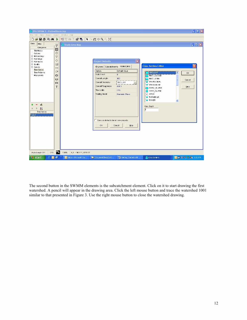
12

The second button in the SWMM elements is the subcatchment element. Click on it to start drawing the first

watershed. A pencil will appear in the drawing area. Click the left mouse button and trace the watershed 1001

similar to that presented in Figure 3. Use the right mouse button to close the watershed drawing.

13

In the main toolbar, use the selector, the black arrow to select elements on the main toolbar. Now click on the

blinking square inside the watershed. Assign the name, description and tag fields “1001”, without the quotes.

Complete the area, width and slope information for this watershed from Table 1. Check that the infiltration

information is correct and close the window.

14

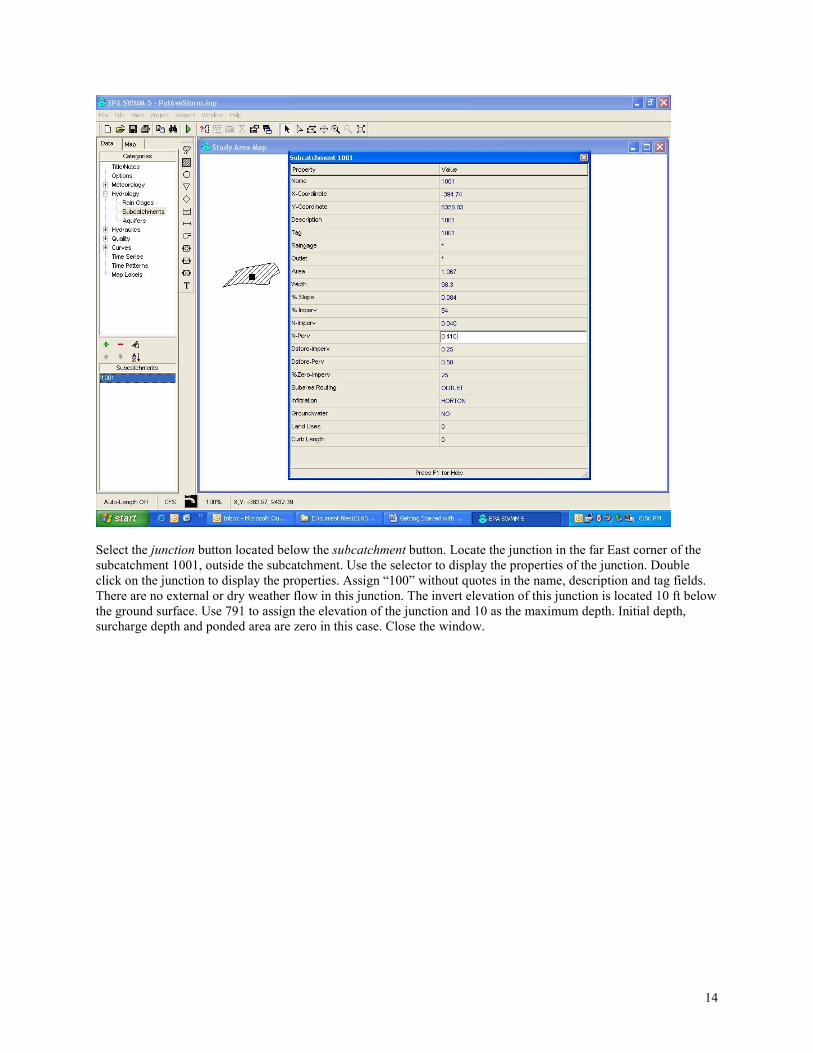
Select the junction button located below the subcatchment button. Locate the junction in the far East corner of the

subcatchment 1001, outside the subcatchment. Use the selector to display the properties of the junction. Double

click on the junction to display the properties. Assign “100” without quotes in the name, description and tag fields.

There are no external or dry weather flow in this junction. The invert elevation of this junction is located 10 ft below

the ground surface. Use 791 to assign the elevation of the junction and 10 as the maximum depth. Initial depth,

surcharge depth and ponded area are zero in this case. Close the window.

15

Double click again in the square located inside the subcatchment. Assign “100” without quotes to the field outlet.

This will indicate that the water produced in this subcatchment will reach the first junction. Close the window. A

dotted line will appear between the square and the junction.

Now a raingage will be created. Click on the button located above the watershed button. It is similar to a cloud

raining. Locate the raingage as shown below.

16

Use the selector from the main toolbar. Double click on the raingage to display its properties. Assign “1” without

quotes to the name, description and tag fields. Click now on the series name. A drop-down menu will appear, select

“Type II”. Close the window. Return to the subcatchment and edit the properties, including selecting “cumulative”

as the data format (the rain is presented in this file as accumulative volumes). Click on the raingage field. A drop

down menu will appear, select 1. Close the window. (Have you saved the project recently?)

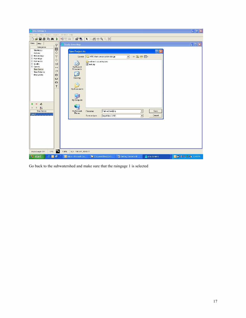
17

Go back to the subwatershed and make sure that the raingage 1 is selected

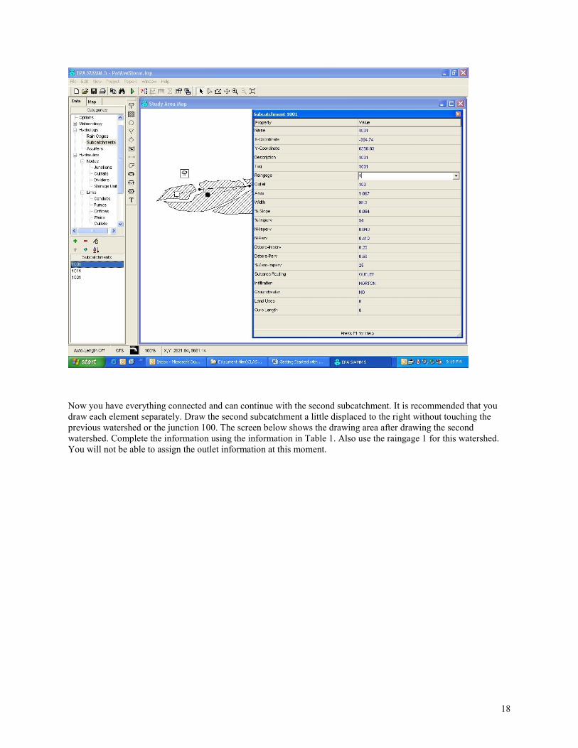
18

Now you have everything connected and can continue with the second subcatchment. It is recommended that you

draw each element separately. Draw the second subcatchment a little displaced to the right without touching the

previous watershed or the junction 100. The screen below shows the drawing area after drawing the second

watershed. Complete the information using the information in Table 1. Also use the raingage 1 for this watershed.

You will not be able to assign the outlet information at this moment.

19

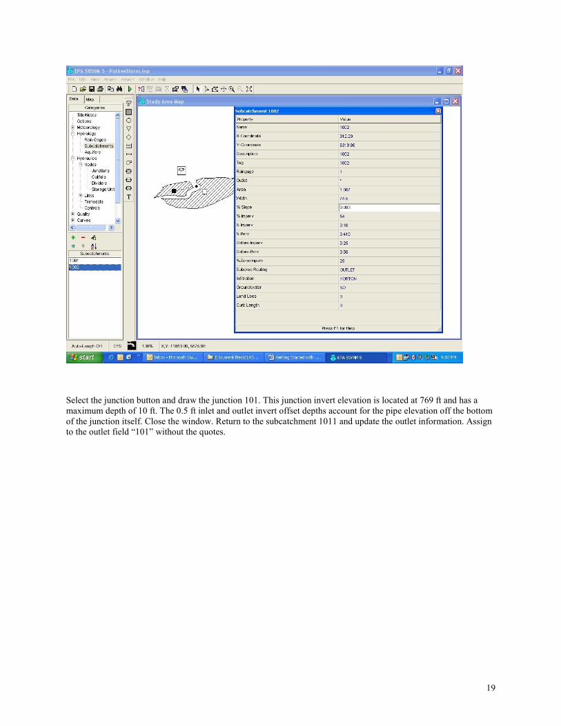
Select the junction button and draw the junction 101. This junction invert elevation is located at 769 ft and has a

maximum depth of 10 ft. The 0.5 ft inlet and outlet invert offset depths account for the pipe elevation off the bottom

of the junction itself. Close the window. Return to the subcatchment 1011 and update the outlet information. Assign

to the outlet field “101” without the quotes.

20

To create the conduit between the junctions 100 and 101, select the seventh button in the SWMM elements toolbar.

Click on the junction 100 and in the junction 101 to create the pipe. Use the selector. Double click on the conduit to

display the properties. You can also click on the little yellow hand located on the properties window. Assign “1000”

without the quotes to the name, description and tag field. Use Table 3 to complete the information of the conduit.

Now create the last watershed using the watershed button and use the information from Table 1 to complete the

required data.

21

22

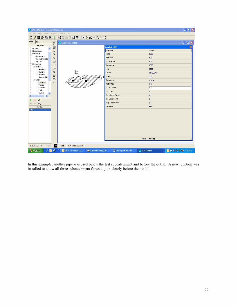
In this example, another pipe was used below the last subcatchment and before the outfall. A new junction was

installed to allow all three subcatchment flows to join clearly before the outfall.

23

24

The last Junction will be modeled as an outfall. Select the fourth element on the SWMM elements toolbar. The

outfall element is located below the junction element. Display its properties. Assign “103” without quotes in the

name, description and tag fields. Assign an invert elevation of 745 ft. There is no tide gate. It is modeled as a free

discharge. The last element is the pipe1003, create this element and update the information using Tables 1, 2 and 3.

25

The rain file used with the raingage is a type II cumulative distribution for a 6.9 inch rain, the “25-yr” recurrence

storm for Birmingham. Different files are needed for each rain depth. A set of standard rain files are located on the

class web site at: www.eng.ua.edu/~rpitt under classes. The files can be modified using Excel. The files are ascii

format (*.txt). Make sure the format is correct. Some problems with Excel is that the SWMM data format MM-DD-

YYYY is not available, and Excel “automatically” converts them to MM/DD/YYYY. The replace function does not

work, as the format is set. If the “normal” format for the cell is used, the “negative” signs transform the values. In

many cases, quotes are also placed on each line, further confusing SWMM. It is best to multiply the rain depths in

Excel, and save as a text file. Then open the file in Notepad and then do a “replace all” command to change the date

format. Finally, save the file before importing into SWMM. The same rain gage and rain event is used for each

subcatchment in this example, but it is possible to have different rain gages to reflect varying rain conditions

throughout an area.

At any time, it is possible to press the F1 key for context-sensitive help.

26

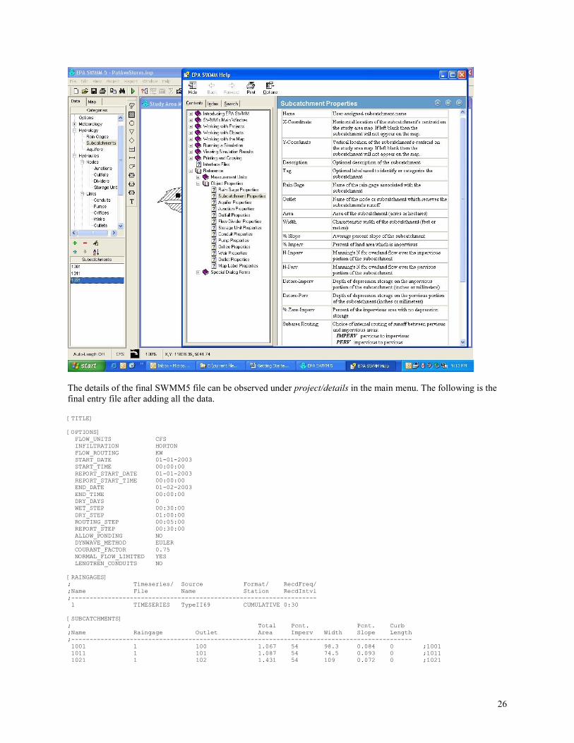
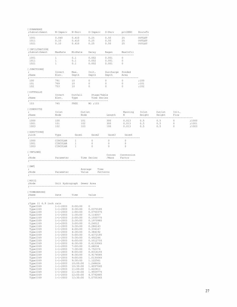
The details of the final SWMM5 file can be observed under project/details in the main menu. The following is the

final entry file after adding all the data.

[TITLE] [OPTIONS] FLOW_UNITS CFS INFILTRATION HORTON FLOW_ROUTING KW START_DATE 01-01-2003 START_TIME 00:00:00 REPORT_START_DATE 01-01-2003 REPORT_START_TIME 00:00:00 END_DATE 01-02-2003 END_TIME 00:00:00 DRY_DAYS 0 WET_STEP 00:30:00 DRY_STEP 01:00:00 ROUTING_STEP 00:05:00 REPORT_STEP 00:30:00 ALLOW_PONDING NO DYNWAVE_METHOD EULER COURANT_FACTOR 0.75 NORMAL_FLOW_LIMITED YES LENGTHEN_CONDUITS NO [RAINGAGES] ; Timeseries/ Source Format/ RecdFreq/ ;Name File Name Station RecdIntvl ;------------------------------------------------------------------- 1 TIMESERIES TypeII69 CUMULATIVE 0:30 [SUBCATCHMENTS] ; Total Pcnt. Pcnt. Curb ;Name Raingage Outlet Area Imperv Width Slope Length ;--------------------------------------------------------------------------------------------- 1001 1 100 1.067 54 98.3 0.084 0 ;1001 1011 1 101 1.087 54 74.5 0.093 0 ;1011 1021 1 102 1.431 54 109 0.072 0 ;1021

27

[SUBAREAS] ;Subcatchment N-Imperv N-Perv S-Imperv S-Perv pctZERO RouteTo ;------------------------------------------------------------------------------- 1001 0.040 0.410 0.25 0.50 25 OUTLET 1011 0.10 0.410 0.25 0.50 25 OUTLET 1021 0.10 0.410 0.25 0.50 25 OUTLET [INFILTRATION] ;Subcatchment MaxRate MinRate Decay Regen MaxInfil ;--------------------------------------------------------------------- 1001 1 0.1 0.002 0.001 0 1011 1 0.1 0.002 0.001 0 1021 1 0.1 0.002 0.001 0 [JUNCTIONS] ; Invert Max. Init. Surcharge Ponded ;Name Elev. Depth Depth Depth Area ;------------------------------------------------------------------------ 100 791 10 0 0 0 ;100 101 769 10 0 0 0 ;101 102 753 10 0 0 0 ;102 [OUTFALLS] ; Invert Outfall Stage/Table ;Name Elev. Type Time Series ;---------------------------------------------------- 103 745 FREE NO ;103 [CONDUITS] ; Inlet Outlet Manning Inlet Outlet Init. ;Name Node Node Length N Height Height Flow ;------------------------------------------------------------------------------------------------------------ 1000 100 101 300 0.013 0.5 0.5 0 ;1000 1001 101 102 300 0.013 0.5 0.5 0 ;1001 1003 102 103 100 0.013 0.5 0.5 0 ;1003 [XSECTIONS] ;Link Type Geom1 Geom2 Geom3 Geom4 ;------------------------------------------------------------------------- 1000 CIRCULAR 1 0 0 0 1001 CIRCULAR 1 0 0 0 1003 CIRCULAR 1 0 0 0 [INFLOWS] ; Concen Conversion ;Node Parameter Time Series /Mass Factor ;---------------------------------------------------------------------- [DWF] ; Average Time ;Node Parameter Value Patterns ;----------------------------------------------------- [RDII] ;Node Unit Hydrograph Sewer Area ;-------------------------------------------- [TIMESERIES] ;Name Date Time Value ;------------------------------------------------- ;Type II 6.9 inch rain TypeII69 1-1-2003 0:00:00 0 TypeII69 1-1-2003 0:30:00 0.0370185 TypeII69 1-1-2003 1:00:00 0.0750375 TypeII69 1-1-2003 1:30:00 0.114057 TypeII69 1-1-2003 2:00:00 0.1550775 TypeII69 1-1-2003 2:30:00 0.1970985 TypeII69 1-1-2003 3:00:00 0.24012 TypeII69 1-1-2003 3:30:00 0.286143 TypeII69 1-1-2003 4:00:00 0.334167 TypeII69 1-1-2003 4:30:00 0.384192 TypeII69 1-1-2003 5:00:00 0.4372185 TypeII69 1-1-2003 5:30:00 0.492246 TypeII69 1-1-2003 6:00:00 0.5512755 TypeII69 1-1-2003 6:30:00 0.6133065 TypeII69 1-1-2003 7:00:00 0.68034 TypeII69 1-1-2003 7:30:00 0.752376 TypeII69 1-1-2003 8:00:00 0.8314155 TypeII69 1-1-2003 8:30:00 0.9174585 TypeII69 1-1-2003 9:00:00 1.0135065 TypeII69 1-1-2003 9:30:00 1.122561 TypeII69 1-1-2003 10:00:00 1.248624 TypeII69 1-1-2003 10:30:00 1.4097045 TypeII69 1-1-2003 11:00:00 1.622811 TypeII69 1-1-2003 11:30:00 1.9559775 TypeII69 1-1-2003 12:00:00 4.5792885 TypeII69 1-1-2003 12:30:00 5.0755365

28

TypeII69 1-1-2003 13:00:00 5.332665 TypeII69 1-1-2003 13:30:00 5.5157565 TypeII69 1-1-2003 14:00:00 5.6598285 TypeII69 1-1-2003 14:30:00 5.7858915 TypeII69 1-1-2003 15:00:00 5.894946 TypeII69 1-1-2003 15:30:00 5.9899935 TypeII69 1-1-2003 16:00:00 6.0760365 TypeII69 1-1-2003 16:30:00 6.1540755 TypeII69 1-1-2003 17:00:00 6.2261115 TypeII69 1-1-2003 17:30:00 6.2921445 TypeII69 1-1-2003 18:00:00 6.355176 TypeII69 1-1-2003 18:30:00 6.4142055 TypeII69 1-1-2003 19:00:00 6.469233 TypeII69 1-1-2003 19:30:00 6.521259 TypeII69 1-1-2003 20:00:00 6.571284 TypeII69 1-1-2003 20:30:00 6.619308 TypeII69 1-1-2003 21:00:00 6.6643305 TypeII69 1-1-2003 21:30:00 6.7083525 TypeII69 1-1-2003 22:00:00 6.749373 TypeII69 1-1-2003 22:30:00 6.7903935 TypeII69 1-1-2003 23:00:00 6.829413 TypeII69 1-1-2003 23:30:00 6.867432 TypeII69 1-2-2003 0:00:00 6.9 [REPORT] CONTROLS NO [COORDINATES] ;Node X-Coord Y-Coord 100 567.61 6560.93 101 2704.51 6711.19 102 6060.10 7262.10 103 6944.91 7262.10 [VERTICES] ;Link X-Coord Y-Coord [Polygons] ;Subcatchment X-Coord Y-Coord 1001 -851.42 6510.85 1001 -884.81 6444.07 1001 -934.89 6393.99 1001 -984.97 6327.21 1001 -1068.45 6260.43 1001 -1135.23 6176.96 1001 -1202.00 6126.88 1001 -1268.78 6060.10 1001 -1202.00 6076.79 1001 -1101.84 6110.18 1001 -984.97 6126.88 1001 -818.03 6160.27 1001 -584.31 6160.27 1001 -400.67 6160.27 1001 -183.64 6143.57 1001 50.08 6143.57 1001 116.86 6160.27 1001 116.86 6210.35 1001 133.56 6293.82 1001 183.64 6360.60 1001 250.42 6410.68 1001 400.67 6477.46 1001 417.36 6494.16 1001 383.97 6577.63 1001 367.28 6627.71 1001 333.89 6677.80 1001 250.42 6777.96 1001 183.64 6777.96 1001 -267.11 6694.49 1001 -634.39 6627.71 1001 -918.20 6510.85 1011 550.92 6777.96 1011 567.61 6744.57 1011 584.31 6711.19 1011 651.09 6661.10 1011 751.25 6594.32 1011 751.25 6494.16 1011 701.17 6427.38 1011 667.78 6410.68 1011 550.92 6360.60 1011 450.75 6327.21 1011 400.67 6310.52 1011 383.97 6277.13 1011 350.58 6227.05 1011 317.20 6143.57 1011 250.42 6060.10 1011 133.56 6026.71 1011 116.86 6026.71

29

1011 116.86 6026.71 1011 16.69 6026.71 1011 -150.25 6026.71 1011 -367.28 6026.71 1011 -534.22 6026.71 1011 -667.78 6026.71 1011 -801.34 6026.71 1011 -884.81 6043.41 1011 -951.59 6043.41 1011 -834.72 5976.63 1011 -767.95 5909.85 1011 -684.47 5809.68 1011 -601.00 5759.60 1011 -534.22 5759.60 1011 -517.53 5759.60 1011 -434.06 5709.52 1011 -317.20 5659.43 1011 -166.94 5642.74 1011 -33.39 5642.74 1011 116.86 5626.04 1011 233.72 5609.35 1011 450.75 5609.35 1011 584.31 5609.35 1011 818.03 5642.74 1011 1051.75 5726.21 1011 1302.17 5809.68 1011 1385.64 5859.77 1011 1602.67 5976.63 1011 1619.37 5976.63 1011 1769.62 6043.41 1011 1886.48 6110.18 1011 1986.64 6126.88 1011 2070.12 6193.66 1011 2136.89 6260.43 1011 2186.98 6293.82 1011 2237.06 6343.91 1011 2270.45 6410.68 1011 2320.53 6460.77 1011 2337.23 6477.46 1011 2387.31 6494.16 1011 2470.78 6560.93 1011 2487.48 6560.93 1011 2504.17 6661.10 1011 2487.48 6727.88 1011 2470.78 6761.27 1011 2454.09 6794.66 1011 2454.09 6811.35 1011 2353.92 6878.13 1011 2270.45 6944.91 1011 2253.76 6928.21 1011 2020.03 6894.82 1011 2003.34 6894.82 1011 1886.48 6928.21 1011 1836.39 6944.91 1011 1702.84 6944.91 1011 1452.42 6944.91 1011 1368.95 6928.21 1011 1268.78 6911.52 1011 1101.84 6911.52 1011 951.59 6911.52 1011 834.72 6928.21 1011 701.17 6861.44 1011 550.92 6828.05 1011 550.92 6811.35 1011 550.92 6811.35 1021 2487.48 6978.30 1021 2520.87 6994.99 1021 2570.95 6978.30 1021 2621.04 6978.30 1021 2704.51 6994.99 1021 2804.67 7011.69 1021 2971.62 7045.08 1021 3088.48 7078.46 1021 3439.07 7178.63 1021 3555.93 7228.71 1021 3856.43 7295.49 1021 4173.62 7295.49 1021 4307.18 7295.49 1021 4373.96 7295.49 1021 4574.29 7295.49 1021 4607.68 7295.49 1021 4791.32 7312.19 1021 4841.40 7312.19 1021 5075.13 7345.58 1021 5375.63 7378.96 1021 5509.18 7378.96 1021 5592.65 7362.27 1021 5626.04 7328.88

30

1021 5776.29 7245.41 1021 5809.68 7178.63 1021 5809.68 7011.69 1021 5792.99 6928.21 1021 5742.90 6727.88 1021 5709.52 6644.41 1021 5626.04 6460.77 1021 5575.96 6427.38 1021 5475.79 6393.99 1021 5375.63 6393.99 1021 5275.46 6393.99 1021 5208.68 6377.30 1021 5158.60 6360.60 1021 5075.13 6310.52 1021 4974.96 6227.05 1021 4858.10 6110.18 1021 4824.71 6093.49 1021 4257.10 5809.68 1021 3856.43 5692.82 1021 3606.01 5592.65 1021 3422.37 5592.65 1021 3055.09 5525.88 1021 2938.23 5525.88 1021 2704.51 5525.88 1021 2353.92 5525.88 1021 2120.20 5509.18 1021 1752.92 5509.18 1021 1669.45 5509.18 1021 1218.70 5592.65 1021 1135.23 5626.04 1021 1135.23 5626.04 1021 1151.92 5642.74 1021 1235.39 5692.82 1021 1335.56 5742.90 1021 1402.34 5792.99 1021 1485.81 5826.38 1021 1636.06 5859.77 1021 1719.53 5926.54 1021 1869.78 5993.32 1021 1953.26 6060.10 1021 2136.89 6143.57 1021 2337.23 6260.43 1021 2420.70 6327.21 1021 2520.87 6393.99 1021 2554.26 6444.07 1021 2621.04 6460.77 1021 2704.51 6494.16 1021 2838.06 6577.63 1021 2871.45 6627.71 1021 2821.37 6711.19 1021 2754.59 6811.35 1021 2687.81 6828.05 1021 2604.34 6811.35 1021 2420.70 7028.38 [SYMBOLS] ;Gage X-Coord Y-Coord 1 -66.78 7228.71 [BACKDROP] DIMENSIONS 0.00 0.00 10000.00 10000.00 UNITS None FILE "" OFFSET 0.00 0.00 SCALING 0.00 0.00

Now you can run the model. In the main toolbar, click the seventh button from the left. The symbol is a green

triangle like a play button. If the run was successful, a window will be displayed showing the successful run label.

31

Observing the Results It is possible to observe the results under report/status in the main menu. An example of the results follows.

32

EPA STORM WATER MANAGEMENT MODEL - VERSION 5.0E (Build 1/23/04) ----------------------------------------------- **************** Analysis Options **************** Flow Units .............. CFS Infiltration Method ..... HORTON Flow Routing Method ..... KW Starting Date ........... JAN-01-2003 00:00:00 Ending Date ............. JAN-02-2003 00:00:00 Wet Time Step ........... 00:30:00 Dry Time Step ........... 01:00:00 Routing Time Step ....... 00:05:00 Report Time Step ........ 00:30:00 ***************** Volume Depth Runoff Continuity acre-feet inches ***************** --------- ------- Total Precipitation ..... 2.061 6.900 Total Losses ............ 0.321 1.074 Total Runoff ............ 1.609 5.385 Initial Storage ......... 0.000 0.000 Final Storage ........... 0.161 0.538 Continuity Error (%) .... -1.409

33

************************* Volume Volume Flow Transport Continuity acre-feet Mgallons ************************* --------- --------- Dry Weather Inflow ...... 0.000 0.000 Wet Weather Inflow ...... 1.602 0.522 Groundwater Inflow ...... 0.000 0.000 RDII Inflow ............. 0.000 0.000 External Inflow ......... 0.000 0.000 External Outflow ........ 1.602 0.522 Initial Stored Volume ... 0.000 0.000 Final Stored Volume ..... 0.000 0.000 Continuity Error (%) .... -0.003 ****************** Node Depth Summary ****************** ---------------------------------------------------------------------------------------- Average Maximum Time of Max Average Total Fraction Depth Depth Occurrence Depth Minutes Courant Node Feet Feet days hr:min Change Flooded Critical ---------------------------------------------------------------------------------------- JUNCTION 100 0.58 0.92 0 12:30 0.0045 0 0.00 JUNCTION 101 0.63 1.16 0 12:30 0.0060 0 0.00 JUNCTION 102 0.65 1.30 0 12:30 0.0069 0 0.00 OUTFALL 103 0.00 0.00 0 00:00 0.0000 0 0.00 ******************** Conduit Flow Summary ******************** --------------------------------------------------------------------------------------- Maximum Time of Max Maximum Time of Max Maximum Total Flow Occurrence Velocity Occurrence /Design Minutes Conduit CFS days hr:min ft/sec days hr:min Flow Surcharged --------------------------------------------------------------------------------------- 1000 3.60e+00 0 12:30 11.38 0 12:30 0.37 0 1001 6.31e+00 0 12:30 11.55 0 12:30 0.77 0 1003 9.83e+00 0 12:30 14.61 0 12:30 0.98 0 Analysis begun: Wed Apr 28 15:12:02 2004

34

Analysis ended: Wed Apr 28 15:12:02 2004

Click on the plot icon (the 9th

from the left on the top tool bar) and select the type of graph and location where

viewing is desired. The following example has “Links” and “Depth” selected in order to plot the depth of flow in the

pipes to visually observe if any pipes surcharged. After these two selections are made, use the selection arrow tool to

click on the links desired to be displayed, and click on the “+” icon in the selection box. Repeat for each link

desired, the click OK for the plot.

35

This plot shows that the most downstream pipe (link 1003) has the deepest flow and is at about 0.8 ft, less than then

the 1 ft pipe diameter. Therefore, no surcharging occurs in these pipes. A similar plot can be created for the nodes

which would be especially important if surcharging does occur to see how far the water rises in the manholes. Recall

that the offset depth for the inlets and outlets for the nodes was 0.5 ft in this example, so the depth can be as great as

1.5 ft before surcharging occurs.

Another option is to show the results in a profile. In the main menu, select Report/graph/profile. The following

figure shows the profile dialog box, with the start and end node selected. After they are selected, the “find path”

button is clicked and the links in the profile are automatically displayed. The click OK to display the profile.

36

37

The animator option is used to display how the profile changes during the simulation. The static plot shows the

depths at the designated time indicated in the lower right-hand corner of the figure. In the above case, water is

shown for the 0.5 ft in the bottom of each node, but none in the pipe. In order to operate the animator, select the drop

down “view/toolbars/animator” option, as indicated below.

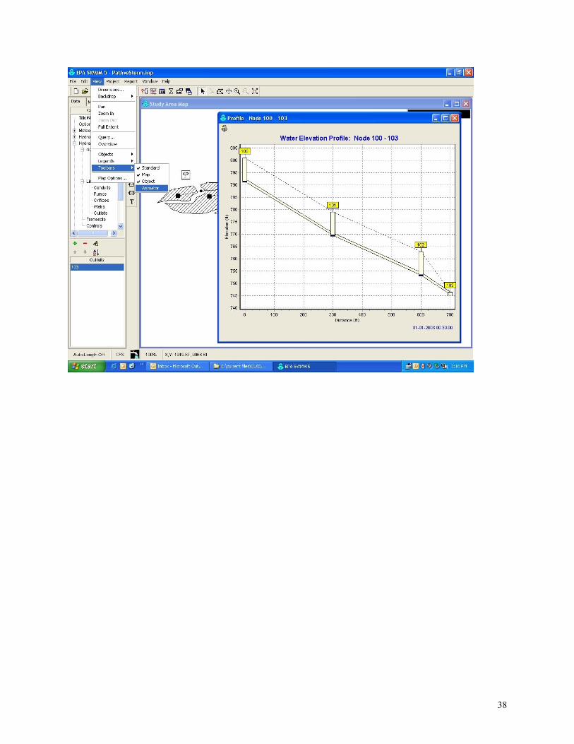
38

39

The lower bar in the animator increases or decreases the speed of the simulation. The left arrow rewinds the

simulation and the right button plays it. The above figure shows the depth at 14:00, with water flowing through the

system. It is difficult to see the water depth in the plotted pipes because of the thinness of the pipes. However, it is

easy to see surcharging conditions during excessive rains.

The results can be observed also in a table. Go to Report/table/by variable in the main menu. Select as object

category: links and as variable: flow. On the map, click conduit 1000, now click the plus sign in the table by

variable window. Now click on the conduit 1001 and click the plus sign to add it to the table. Click OK and the

results will be displayed in a table.

40

41

Long-term Continuous Simulation It is possible to use a variety of rain files with SWMM5. The following illustrates the use of a four month period of

rains monitored at the University of Alabama for this site. The first step is to import the new rain file (4 months of 5

minute observations).

42

43

44

Next, the rain gage needs to be edited for the correct file name and file type. Again, this is a time series of volume

data, collected at 5 minute intervals.

45

It is also necessary to edit the simulation options to reflect the new start and end dates for the simulation.

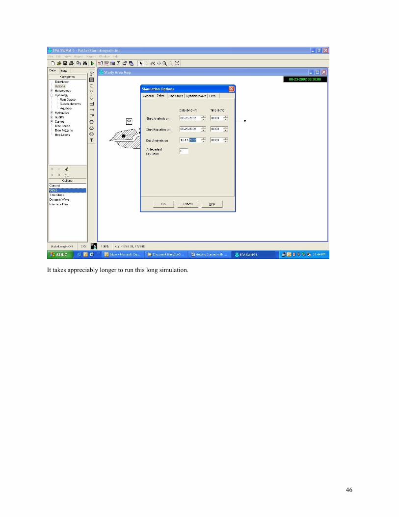
46

It takes appreciably longer to run this long simulation.

47

48

Again, the plotting options need to have the observation locations selected, but using the selector arrow in SWMM

to click on the appropriate link, and then clicking on the “+” sign. Multiple elements of the same type can be

selected for plotting together.

49

50

“Hello World” Pat Avenue Sanitary Drainage Design Example It is easy to also design a sanitary drainage system using SWMM5. In this example, we will use the same location.

The sanitary sewer is another pipe located on the other side of the road, 3 ft below the storm sewer pipe. Three pipes

and three upper manholes are required in this design. Sewage discharges from the residents in the upper part of the

street will be to pipe 2000. The following shows the location of the manholes and pipes in the design

The description of the sewage discharge and the subareas contribution is shown in Table 4.

51

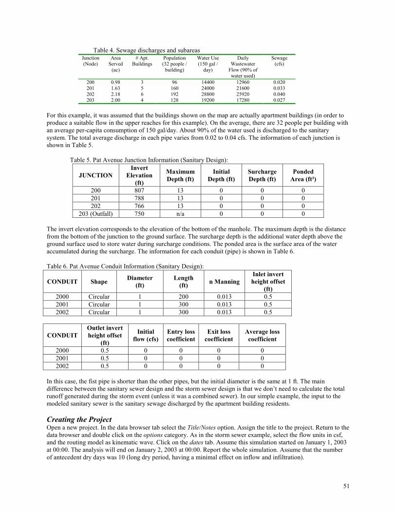
Table 4. Sewage discharges and subareas Junction (Node)

Area Served

(ac)

# Apt. Buildings

Population (32 people /

building)

Water Use (150 gal /

day)

Daily Wastewater

Flow (90% of

water used)

Sewage (cfs)

200 0.98 3 96 14400 12960 0.020

201 1.63 5 160 24000 21600 0.033

202 2.18 6 192 28800 25920 0.040 203 2.00 4 128 19200 17280 0.027

For this example, it was assumed that the buildings shown on the map are actually apartment buildings (in order to

produce a suitable flow in the upper reaches for this example). On the average, there are 32 people per building with

an average per-capita consumption of 150 gal/day. About 90% of the water used is discharged to the sanitary

system. The total average discharge in each pipe varies from 0.02 to 0.04 cfs. The information of each junction is

shown in Table 5.

Table 5. Pat Avenue Junction Information (Sanitary Design):

JUNCTION

Invert

Elevation

(ft)

Maximum

Depth (ft)

Initial

Depth (ft)

Surcharge

Depth (ft)

Ponded

Area (ft²)

200 807 13 0 0 0

201 788 13 0 0 0

202 766 13 0 0 0

203 (Outfall) 750 n/a 0 0 0

The invert elevation corresponds to the elevation of the bottom of the manhole. The maximum depth is the distance

from the bottom of the junction to the ground surface. The surcharge depth is the additional water depth above the

ground surface used to store water during surcharge conditions. The ponded area is the surface area of the water

accumulated during the surcharge. The information for each conduit (pipe) is shown in Table 6.

Table 6. Pat Avenue Conduit Information (Sanitary Design):

CONDUIT Shape Diameter

(ft)

Length

(ft) n Manning

Inlet invert

height offset

(ft)

2000 Circular 1 200 0.013 0.5

2001 Circular 1 300 0.013 0.5

2002 Circular 1 300 0.013 0.5

CONDUIT

Outlet invert

height offset

(ft)

Initial

flow (cfs)

Entry loss

coefficient

Exit loss

coefficient

Average loss

coefficient

2000 0.5 0 0 0 0

2001 0.5 0 0 0 0

2002 0.5 0 0 0 0

In this case, the fist pipe is shorter than the other pipes, but the initial diameter is the same at 1 ft. The main

difference between the sanitary sewer design and the storm sewer design is that we don’t need to calculate the total

runoff generated during the storm event (unless it was a combined sewer). In our simple example, the input to the

modeled sanitary sewer is the sanitary sewage discharged by the apartment building residents.

Creating the Project Open a new project. In the data browser tab select the Title/Notes option. Assign the title to the project. Return to the

data browser and double click on the options category. As in the storm sewer example, select the flow units in csf,

and the routing model as kinematic wave. Click on the dates tab. Assume this simulation started on January 1, 2003

at 00:00. The analysis will end on January 2, 2003 at 00:00. Report the whole simulation. Assume that the number

of antecedent dry days was 10 (long dry period, having a minimal effect on inflow and infiltration).

52

Click on the Time Steps tab. In this example, the rain file will not be included, leave the default value or 30 minutes.

The dry weather processes is simulated, use 1 hour time step in this case. Select a 5-minute routing time step and a

15-minute reporting time step. The dynamic wave and Interface files tabs are not used. Click ok to accept the values.

Now you will import a time series describing the sanitary sewage discharges in the study area. In the data browser,

select the Time Patterns option and in the properties area add a new series. In the name field, assign the name

“patavam” without quotes and spaces. Select type AM. Describe the time pattern, for example “AM Pat Avenue

Pattern”. The following figure shows the 12 percentages of the average flow used before noon: 68, 57, 49, 75, 100,

132, 170, 208, 198, 151, 94, and 75. Create a second pattern called “patavpm” for the PM part of the day. The

percentages are: 79, 81, 91, 98, 100, 102, 83, 85, 87, 79, 70, and 72. These values are the percentages of the basic

average hourly flow value produced by the residents.

Go to the main menu and select: Project/defaults. Click on the Nodes/Links tab. Assign 0 to the node invert and 300

ft to the conduit length. The pipes are circular with a roughness coefficient of 0.013. The flow units are in cfs and

the routing model is kinematic wave. Click O.K. to accept the changes.

Now you can start to draw the pipes, nodes and outfall. Notice that in this case there are three pipes, three junctions

and an outfall. Include all the required information using tables 4, 5 and 6. Start with the junctions and the outfall.

Double click on the first junction to display its properties. Rename the node as 200. Click on inflows. A window will

appear. Select the Dry Weather tab. Select constituent as Flow, the average values is shown in table 4. This flow is

0.020 cfs for the first junction. Assign the time patterns for the AM and PM part of the day. Click OK. Complete the

required information for this node. Create the other two nodes and the outfall. Fill in the required information from

tables 4, 5 and 6. The outfall is free (again, there is no a tide gate at the end). Use the T button in the drawing

elements to add text labels to the map and identify each element. The following figure shows the final sketch for the

layout for the sanitary sewer design.

53

Check in the main menu, project/details that the input file is complete, You can also open your input file with any

word processor. In this moment you are ready to run the program. Compare your file with the following text file: [TITLE] Sanitary Sewer Design Example Pat Avenue Alex Maestre - University of Alabama [OPTIONS] FLOW_UNITS CFS INFILTRATION HORTON FLOW_ROUTING KW START_DATE 01-01-2003 START_TIME 00:00:00 REPORT_START_DATE 01-01-2003 REPORT_START_TIME 00:00:00 END_DATE 01-02-2003 END_TIME 00:00:00 DRY_DAYS 10 WET_STEP 00:15:00 DRY_STEP 01:00:00 ROUTING_STEP 00:05:00 REPORT_STEP 00:15:00 ALLOW_PONDING YES DYNWAVE_METHOD EULER COURANT_FACTOR 0.75 NORMAL_FLOW_LIMITED YES LENGTHEN_CONDUITS NO [JUNCTIONS] ; Invert Max. Init. Surcharge Ponded ;Name Elev. Depth Depth Depth Area ;------------------------------------------------------------------------ 200 807 13 0 0 0 201 788 13 0 0 0 202 766 13 0 0 0

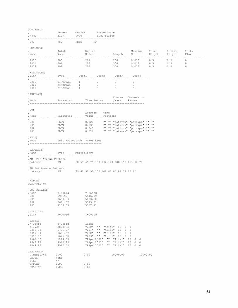
54

[OUTFALLS] ; Invert Outfall Stage/Table ;Name Elev. Type Time Series ;---------------------------------------------------- 203 750 FREE NO [CONDUITS] ; Inlet Outlet Manning Inlet Outlet Init. ;Name Node Node Length N Height Height Flow ;------------------------------------------------------------------------------------------------------------ 2000 200 201 200 0.013 0.5 0.5 0 2001 201 202 300 0.013 0.5 0.5 0 2002 202 203 300 0.013 0.5 0.5 0 [XSECTIONS] ;Link Type Geom1 Geom2 Geom3 Geom4 ;------------------------------------------------------------------------- 2000 CIRCULAR 1 0 0 0 2001 CIRCULAR 1 0 0 0 2002 CIRCULAR 1 0 0 0 [INFLOWS] ; Concen Conversion ;Node Parameter Time Series /Mass Factor ;---------------------------------------------------------------------- [DWF] ; Average Time ;Node Parameter Value Patterns ;----------------------------------------------------- 200 FLOW 0.020 "" "" "patavam" "patavpm" "" "" 201 FLOW 0.033 "" "" "patavam" "patavpm" "" "" 202 FLOW 0.040 "" "" "patavam" "patavpm" "" "" 203 FLOW 0.027 "" "" "patavam" "patavpm" "" "" [RDII] ;Node Unit Hydrograph Sewer Area ;-------------------------------------------- [PATTERNS] ;Name Type Multipliers ;--------------------------------------- ;AM Pat Avenue Pattern patavam AM 68 57 49 75 100 132 170 208 198 151 94 75 ;PM Pat Avenue Pattern patavpm PM 79 81 91 98 100 102 83 85 87 79 70 72 [REPORT] CONTROLS NO [COORDINATES] ;Node X-Coord Y-Coord 200 699.52 5516.69 201 3688.39 5453.10 202 6661.37 5373.61 203 9157.39 5357.71 [VERTICES] ;Link X-Coord Y-Coord [LABELS] ;X-Coord Y-Coord Label 413.35 5898.25 "200" "" "Arial" 10 0 0 3386.33 5771.07 "201" "" "Arial" 10 0 0 6359.30 5691.57 "202" "" "Arial" 10 0 0 8855.33 5675.68 "203" "" "Arial" 10 0 0 1669.32 5214.63 "Pipe 2000" "" "Arial" 10 0 0 4642.29 4960.25 "Pipe 2001" "" "Arial" 10 0 0 7344.99 4912.56 "Pipe 2002" "" "Arial" 10 0 0 [BACKDROP] DIMENSIONS 0.00 0.00 10000.00 10000.00 UNITS None FILE "" OFFSET 0.00 0.00 SCALING 0.00 0.00

55

If everything looks fine, run the model. The results from the model should be similar to the following: EPA STORM WATER MANAGEMENT MODEL - VERSION 5.0E (Build 1/23/04) ----------------------------------------------- Sanitary Sewer Design Example Pat Avenue Alex Maestre - University of Alabama **************** Analysis Options **************** Flow Units .............. CFS Flow Routing Method ..... KW Starting Date ........... JAN-01-2003 00:00:00 Ending Date ............. JAN-02-2003 00:00:00 Routing Time Step ....... 00:05:00 Report Time Step ........ 00:15:00 ************************* Volume Volume Flow Transport Continuity acre-feet Mgallons ************************* --------- --------- Dry Weather Inflow ...... 23.869 7.778 Wet Weather Inflow ...... 0.000 0.000 Groundwater Inflow ...... 0.000 0.000 RDII Inflow ............. 0.000 0.000 External Inflow ......... 0.000 0.000 External Outflow ........ 23.865 7.777 Initial Stored Volume ... 0.000 0.000 Final Stored Volume ..... 0.007 0.002 Continuity Error (%) .... -0.011 ****************** Node Depth Summary ****************** ---------------------------------------------------------------------------------------- Average Maximum Time of Max Average Total Fraction Depth Depth Occurrence Depth Minutes Courant Node Feet Feet days hr:min Change Flooded Critical ---------------------------------------------------------------------------------------- JUNCTION 200 0.78 0.93 0 07:05 0.0063 0 0.00 JUNCTION 201 1.04 1.50 0 07:00 0.0128 0 0.00 JUNCTION 202 1.34 1.50 0 04:00 0.0145 0 0.00 OUTFALL 203 0.00 0.00 0 00:00 0.0000 0 0.00 ******************** Conduit Flow Summary ******************** --------------------------------------------------------------------------------------- Maximum Time of Max Maximum Time of Max Maximum Total Flow Occurrence Velocity Occurrence /Design Minutes Conduit CFS days hr:min ft/sec days hr:min Flow Surcharged --------------------------------------------------------------------------------------- 2000 4.20e+00 0 07:05 13.04 0 07:05 0.38 0 2001 9.65e+00 0 07:00 13.97 0 06:05 1.00 120 2002 8.84e+00 0 10:40 11.94 0 20:05 1.07 560 Analysis begun: Sun Apr 25 20:12:34 2004 Analysis ended: Sun Apr 25 20:12:34 2004

The results show that the diameters of pipes 2001 and 2002 are not large enough to transport the flow (they

surcharge). This pipes can be replaced by larger pipes (1.5 ft pipes will be used). The following figure shows the

current results with pipes 1 ft in diameter.

56

The results after enlarging pipes 2001 and 2002 to the next largest commercial pipe size show that pipe 2002 only

reaches 67% of the total capacity during the peak hour so the new design appears to be satisfactory. The following

figure shows the flow depths at each node with pipes 2001 and 2002 enlarged to 2 ft in diameter.

References http://www.epa.gov/ednnrmrl/swmm/beta_test.htm

US EPA, National Risk Management Research Laboratory, Office of Research and Development, (2002). SWMM

Redevelopment Project Plan. Version 5. Water Supply and Water Resources Division.

James, W., W. Huber, R. Pitt, R. Dickinson, and R. James (2002). Water Systems Models, Hydrology. CHI, Guelph

Ontario Canada. 347 pp.

Chow V., (1988). Applied Hydrology. McGraw Hill Book Co. – New York.