![Journal of Computational and Graphical Statistics Volume 12 Issue 1 2003 [Doi 10.2307_1391072] R. J. Bolton and W. J. Krzanowski -- Projection Pursuit Clustering for Exploratory Data](https://static.fdocuments.us/doc/165x107/55cf8fab550346703b9ea2e8/journal-of-computational-and-graphical-statistics-volume-12-issue-1-2003-doi.jpg)
(M) September 1973 A PROJECTION PURSUIT …inspirehep.net/record/81111/files/slac-pub-1312.pdf ·...
39
~LAC-~~~~-1312 (M) September 1973 A PROJECTION PURSUIT ALGORITHM FOR EXPLORATORY DATA ANALYSIS Jerome H. Friedman Stanford Linear Accelerator Center* Stanford, California 94305 and John W. Tukey Princeton University** Princeton, New Jersey 08540 and Bell Laboratories Murray Hill, New Jersey 07974 ABSTRACT An algorithm for the analysis of multivariate data is presented, and discussed in terms of specific examples. The algorithm seeks to find one- and two-dimensional linear projections of multivariate data that are relatively highly revealing. *Supported by the U.S. Atomic Energy Commission under Contract AT(@+3)515. **Prepared in part in connection with research at Princeton University supported by the U.S. Atomic Energy Commission. (Submitted to IEEE Trans. on Computers)
Transcript of (M) September 1973 A PROJECTION PURSUIT …inspirehep.net/record/81111/files/slac-pub-1312.pdf ·...

~LAC-~~~~-1312 (M) September 1973
A PROJECTION PURSUIT ALGORITHM FOR
EXPLORATORY DATA ANALYSIS
Jerome H. Friedman Stanford Linear Accelerator Center*
Stanford, California 94305 and
John W. Tukey Princeton University**
Princeton, New Jersey 08540 and
Bell Laboratories Murray Hill, New Jersey 07974
ABSTRACT
An algorithm for the analysis of multivariate data is
presented, and discussed in terms of specific examples.
The algorithm seeks to find one- and two-dimensional
linear projections of multivariate data that are
relatively highly revealing.
*Supported by the U.S. Atomic Energy Commission under Contract AT(@+3)515.
**Prepared in part in connection with research at Princeton University supported by the U.S. Atomic Energy Commission.
(Submitted to IEEE Trans. on Computers)

KEY PHRASES
Multivariate data analysis Dimensionality reduction
Statistics Clustering
Multidimensional scaling Mappings
Non-parametric pattern recognition

Introduction
Mapping of multivariate data onto low-dimensional manifolds for visual in-
spection is a commonly used technique in data analysis. The discovery of mappings
that reveal the salient features of the multidimensional point swarm is often far
from trivial. Even when every adequate description of the data requires more
variables than can be conveniently perceived (at one time) by humans, it is quite
often still useful to map the data into a lower, humanly perceivable, dimension-
ality where the human gift for pattern recognition can be applied.
While the particular dimension-reducing mapping used may sometimes be in-
fluenced by the nature of the problem at hand, it seems usually to be dictated
by the intuition of the researcher. Potentially useful techniques can be divided
into three classes:
1) Linear dimension-reducers, which can usually be usefully thought
of as projections.
2) Non-linear dimension-reducers that are defined over the whole
high-dimensional space. (N o examples seem as yet to have been
seriously proposed for use in any generality.)
3) Non-linear mappings that are only defined for the given points --
most of these begin with the mutual interpoint distances as the
basic ingredient. (Minimal spanning trees,2 and iterative algor-
ithms for non-linear mappings, 374 are examples. The literature of
clustering techniques is extensive. *I
While the non-linear algorithms have the ability to provide a more faithful
representation of the multidimensional point swarm than the linear methods, they
*See References- 1 and 2 and their references for a.reasonably extensive bibli- ography on clustering techniques.
-l-

can suffer from some serious shortcomings; namely, the resulting mapping is often
difficult to interpret; it cannot be summarized by a few parameters; it only exists
for the data set used in the analysis, so that additional data cannot be identically
mapped; and, for moderate to large data bases, its use is extremely costly in
computational resources (both CPU cycles and memory).
Our attention here is devoted to linear methods, more specifically to those
expressable as projections (though the technique seems extendable to more general
linear methods). Classical linear methods include principal components and linear
factor analysis. Linear methods have the advantages of straight-forward inter-
pretability and computational economy. Linear mappings provide parameters which
are independently useful in the understanding of the data, as well as being de-
fined throughout the space, thus allowing the same mapping to be performed on
additional data that was not part of the original analysis. The disadvantage of
many classical linear methods is that the only property of the point swarm that
is used to determine the mapping is a global one, usually the swarm's variance
along various directions in the multidimensional space. Techniques that, 'like
projection pursuit, combine global and local properties of multivariate point
swarms to obtain useful linear mappings have been proposed by Kruskal. 5,6 Since
projection pursuit uses trimmed global measures, it has the additional advantage
of robustness against outliers.
-2-

Projection Pursuit
This note describes a linear mapping algorithm that uses interpoint dis-
tances as well as the variance of the point swarm to pursue optimum projections.
This projection pursuit algorithm associates with each direction in the multi-
dimensional space, a continuous index that measures its %sefulness" as a pro-
jection axis, and then varies the projection direction so as to maximize this
index. This projection index is sufficiently continuous to allow the use of
sophisticated hill climbing algorithms for the maximization, thus increasing
computational efficiency. (In particular, both Rosenbrock7 and Powell principal
axis8 methods have proved very successful). For complex data structures, several
solutions may exist, and for each of these the projections can be visually in-
spected by the researcher for interpretation and judgment as to their usefulness.
This multiplicity is often important.
Computationally, the projection pursuit (PP) algorithm is considerably more
economical than the non-linear mapping algorithms. Its memory requirements are
simply proportional to the number of data points, N, while the number of CPU
cycles required grows as NlogN for increasing N. This allows the PP algorithm
to be applied to much larger data bases than is possible with nonlinear mapping
algorithms, where both the memory and CPU requirements tend to grow as 8.
Since the mappings are linear, they have the advantages of straightforward
interpretability and convenient summarization. Also, once the parameters that
define a solution projection are obtained, additional data that did not participate
in the search can be mapped onto it. For example, one may apply projection pur-
suit to a data subsample of size Ns. This requires computation proportional to
Ns log Ms. Once a subsample solution projection is found7 the.entire data set
can->be:projected onto it (for inspection by the researcher) with CPU requirements
simply proportional to N.
-3-

When combined with isolation, 9 projection pursuit has been found to be an
effective tool for cluster detection and separation. As projections are found
that separate the data into two or more apparent clusters, the data points in
each cluster can be isolated. The PP-algorithm can then be applied to each
cluster separately, finding new projections that may reveal further clustering
within each isolated data set. These sub-clusters can each be isolated and the
process repeated.
Because of its computational economy, p rejection pursuit can be repeated
many times on the entire data base, or its isolated subsets, making it a feasible
tool for exploratory data analysis. The algorithm has so far been implemented
for projection onto one and two dimensions; however, there is no fundamental
limitation on the dimensionality of the projection space.
The Projection Index
The choice of the intent of the projection index, and to a somewhat lesser
degree the choice of its details, are crucial for the success of the algorithm.
Our choice of intent was motivated by studying the interaction between human
operators and the computer on the PRIM-9 interactive data display system. JJ This
system provides the operator with the ability to rotate the data to any desired
orientation while continuously viewing a two-dimensional projection of the multi-
dimensional data. These rotations are performed in real time and in a continuous
manner under operator control. This gives the operator the ability to perform
manual projection pursuit. That is, by controlling the rotations and viewing
the changing projections, the operator can try to discover those data orienta-
tions (or equivalently projection directions) that reveal to him interesting
structure. It was found that the strategy most frequently employed by researchers
operating the system was to seek out projections that tended to producemany very
small interpointldistances while; at.:-the--same':Jtime3: maintaining the overall spread
of -the ;d,ata. *Such.strategies will, for instance, tend to;concentrate the points
into clusters while, at the same time, separating the clusters.
-4-
The P-indexes we use to express quantitatively such properties of a projection
axis, 2, can be written as a product of two functions
I (2) = s(g) d(i;) (1)
where s(E) measures the spread of the data, and d(E) describes the "local density"
of the points after projection onto 2. For s(e), we take the trimmed standard
deviation of the dtta from the mean as projected onto e;
s(t) = -1
$l-P)N
i ti=pN (q. i; - Xkj2 / (l-2P)Ni
/ i
where (2)
(1-P)N
I Xk = i=pN
TFi.l? / (l-2p)N.
Here N is the total number of data points, and ?i (i=l,N) are the multivariate
vectors representing each of the data points, ordered according to their pro-
jections xi . 2. A small fraction, p, of the points that lie at each of the
extremes of the projection are omitted from both sums. Thus, extreme values of
??i * e do not contribute to s(g), which is thus robust against extreme outliers.
For d(e), we use an average nearness function of the form
N N
d(E) = c c i=l j=l
f(rij) l(R-rij)
where r ij = 1 zp-?j.q
(3)
and l(T)) is unity for positive valued arguments and zero for negative values.
(Thus, the double sum is confined to pairs with 0 5 r.. < R.) The function f(r) 1J
should be monotonically decreasing for increasing r in the range r 5R, reducing
to zero at r=R. This continuity assures maximum smoothness of the objective
function, I(S). -5-

For moderate to large sample size, N, the cutoff radius, R, is usually chosen
so that the average number of points contained within the window, defined by the
step function l(R-r..), is not only a small fraction of N but increases much more 1J
slowly than N, say as log N. After sorting the projected point values, ?i * 2,
the number of operations required to evaluate d(E) [as well as s(6)] is thus about
a fixed multiple of N log N (probably no more than this for large N). Since sorting
requires a number of operations proportional to N log N, the same is true of the
entire evaluation of d(c) and s(E) combined.
Projections onto two dimensions are characterized by two directions 2 and
conveniently taken to be orthogonal with respect to the initially given co-
ordinates and their scales). For this case, equation (2) generalizes to
s(l& = s(6) s(X)
and r.. becomes r l/2
I-J ij = [(qa - Zj.l?'
(2a)
(34
in equation (3).
Repeated application of the algorithm has shown that it is insensitive to
the explicit functional form of f(r) and shows major dependence only on its
characteristic width
f(r)dr. 0
-1 R i R
! rf(r)rdr
r r= 1 I
i J f(r)rdr
0 0
(one dimension) (4)
, (two dimensions) . (44
-6-

It is this characteristic width that seems to define ltlocal" in the search for
maximum local density. Its value establishes the distance in the projected sub-
space over which the local density is averaged, and thus establishes the scale
of density variation to which the algorithm is sensitive. Experimentation has
also shown that when a preferred direction is available, the algorithm is re-
markably stable against small to moderate changes in ?, but it does respond to
large changes in its value (say a few factors of two).
The projection index I(??) [ or I(s,x) for two-dimensional projections]
measures the degree to which the data points in the projection are both concen-
trated locally (d($?).,large),~while, at8~thesame:time, 'expanded globally (s(E) large).
Experience ‘has,.-shown--thatcprojectiops:thatr‘ihave,:this'property.'1o~a large degree
tend.-:8to-be,'those;that:are,most interesting:torresearchersL~-~;Thus;~~it,seems natural
to pursue-those'projections;that-maximize this index.
One-Dimensional Projection Pursuit
The projection index for projection onto a one-dimensional line imbedded in
an n-dimensional space is a function of n-l independent variables that define the
direction of the line, conveniently its direction cosines. These cosines are the
n components of a vector parallel to the line subject to the constraint that the
squares of these components sum to unity. Thus, we seek the maxima of the P-
index, I(s), on the (n-l)-dimensional surface of a sphere of unit radius, Sn(l),
in an n-dimensional Euclidean space.
One technique for accomplishing this is to apply a solid angle transform
(sAT)~~ which reversibly maps such a sphere to an (n-l)-dimensional infinite z.
Euclidean space E n-l (-co,co).(see appendix). This reduces the problem from
finding the maxima of I(s) on the unit sphere in n-dimensions, to finding the
equivalent maxima of I[SAT('$)] in En-'(-co,co). This replacement of the con-
strained optimization problem with a totally unconstrained one, greatly increases
-7-

the stability of the algorithm and simplifies its implementation. The variables
of the search are the n-l SAT parameters, and for any such set of parameters there
exists a unique point on the n-dimensional sphere defined by the n components
of ii.
The computational resources required by projection pursuit are greatly
affected by the algorithm used in the search for the maxima of the. projection
index. Since the number of CPU cycles required to evaluate the P-index for N
data points grows as NlogN, it is important for moderate to large data sets to
employ a search algorithm that requires as few evaluations of the object function
as possible. It is usually the case that the more sophisticated the search al-
gorithm, the smoother the object function is required to be for stability. The
P-index, I(e), as defined above, is remarkably smooth, and both Rosenbrock 12 and
Powell principal axis 13 search algorithms have been successfully applied without
encountering any instability problems. For these algorithms, the number of
objective function evaluations per varied parameter required to find a solution
projection has been found to vary considerably from instance to instance and to
be strongly influenced by the convergence criteria established by the user.
Applying a rather demanding convergence criteria, approximately 15-25 evaluations
per varied parameter were required to achieve a solution. (Stopping when the
P-index changes by only a few percent seems reasonable. A convergence criteria
of one percent was used in all of our applications.)
In order to be useful as a tool for exploratory data analysis on data sets
with complex structure, it is important that the algorithm find several solutions -a ?-,.,. i; that represent potentially informative projections for inspection by the re-
r. searcher. This can be accomplished by applying the algorithm many times with
different starting directions for the search. Useful starting directions in-
clude the larger principal axes of the data set, the original coordinate axes,
and even directions chosen at random. From each starting direction, Es, the
-%-

I
* algorithm finds the solution projection axis, c
S’ corresponding to the first
maximum of the P-index uphill from the starting point. From these searches,
several quit-e-distinct solutions often result..F Each-of.,these ,projections ,can
then be examined_to determine their usefulness! in-datainterpretation.
In order to encourage the algorithm to find additional distinct solutions,
it is useful to be able to reduce the dimensionality of the sphere to be searched.
This can be done by choosing an arbitrary set of directions, {8,}m,, m < n,
which need not be mutually orthogonal, and applying the constraints
It” i=o -G i = 1,m (4)
on the solution direction E*. Possible choices for constraint directions might
be solution directions found on previous searches, or directions that are known
in advance to contain considerable, but well understood, structure. Also, when
the choice of scales for the several coordinates is guided by considerations out-
side the data, one might wish to remove directions with small variance about the
mean, since these directions often provide little information about the structure
of the data. The introduction of each such:eonstraint?directidn reduces,:by+one
the number of search variables, and thus increases the computational efficiency
of the algorithm.
The algorithm can allow for the introduction of an arbitrary number, m < n,
of non-parallel constraint directions. This is accomplished by using Householder
reductions14 to form an orthogonal basis for the (n-m)-dimensional orthogonal
subspace of the m-dimensional subspace spanned by the m constraint vectors
I’il~=l’ The n-m-l search variables are then the solid angle transform param-
eters of the unit sphere in this (n-m)-dimensional space. The transformation
from the original n-dimensional data space proceeds in two steps. First, a
linear dimension reducing transformation to the (n-m)-dimensional complement
subspace, and then the nonlinear SAT that maps the sphere, Sn(gi), to E p-?$).
-9-
Two-Dimensional Projection Pursuit A
The projection index, I(g,&), for a two-dimensional plane imbedded in an
n-dimensional space is defined by eqns 2a, 3 and 3a. This index is a function
of the parameters that define such a plane. Proceeding in analogy
with one-dimensional projection pursuit, one could seek the maximum of I($,;)
with respect to these parameters. The data projected onto the plane represented A*
by the solution vectors, It" and t , can then be inspected by the researcher.
Another useful strategy is to hold one of the directions (for example 2)
constant along some interesting direction, and then seek the maximum of h
with respect to & in? -l(s), the (n-1)-d* imensional subspace orthogonal
This reduces the number of search parameters to n-2. The choice of the
I&G to I?. constant
direction, 2, could be motivated by the problem at hand (like one of the original
or principal axes), or it could be a solution direction found in a one dimensional
projection pursuit.
A third, intermediate, strategy would be to first fix 2 and seek the maxi-
mum of 1(2,x) in 'En-'(s), as described above. Then, holding l fixed at the
solution value Z+, vary G in ‘Zn-l(X*) seeking a further maximum of I(%?,T). This
process of alternately fixing one direction and varying the other in the orthog-
onal subspace of the first, can be repeated until the solution becomes stable. A*
The final directions R* and & are then regarded as defining the solution plane.
This third strategy, while not as completely general as the first, is computationally
much more efficient. This is due to the economies that can be achieved in com-
puting I($?,:), k nowing that one of the directions is constant and that 2-z = 0.
(Using similar criteria for choosing the cutoff radius as that used for one-
dimensional projection pursuit, and sorting the projected values along the constant
direction, allows 1(6,x) to b e evaluated with a number of operations proportional
to N log N.)
As for the one-dimensional case, the two-dimensional P-index, I(%?,:) is
sufficiently smooth to allow the use of sophisticated optimization algorithms.
Also, constraint directions can be introduced in the same manner as described
above for one dimensional projection pursuit.
- 10 -

Some Experimental Results
To illustrate the application of the algorithm, we describe its effect upon
several data sets. The first two are artifically generated so that the results
can be compared with the known data structure. The third is the well known
Iris data used by Fisher-l5 and the fourth is a data set taken from a particle
physics experiment. For these examples, f(r) = R-r, for one-dimensional pro-
jection pursuit (eqn 3), while for two-dimensional projection pursuit (eqn 3a),
f(r) = R2-r2. In both cases R was set to ten percent of the square root of the
data variance along the largest principal axis, and the trimming (eqn 2) was
P = .05.
1) Uniformally Distributed Random Data
To test the effectofprojection pursuit on artificial data having no pre-
ferred projection axes, we generated 975 data points, randomly, from a uniform
distribution inside a lb-dimensional sphere, and repeatedly applied one and two-
dimensional projection pursuit to the sample with different starting directions.
Table 1 shows the results of 2% such trials with one-dimensional projection pur-
suit where the starting directions were the 14 original axes and the 14 principal
axes of the data set. The results of the two-dimensional projection pursuit
tr&als were very similar.
The results shown in Table 1 strongly reflect the uniform nature of the 14-
dimensional data set. The standard deviation of the index values for the starting
directions is less than one percent, while the increase achieved at the solutions
averages four percent. Also, only two searches (runs 13 and 14) appeared to con-
verge to the same solution. The angle between the two directions corresponding
to the largest P-indices found (runs 19 and 21) was 67 degrees. The small in-
crease in the P-index from the starting to the solution directions, indicates
that the algorithm considers these solution directions at most only slightly
better projection axes than the starting directions. Visual inspection of the
data projections verifies this assessment.
- 11 -

2) Gaussian Data Distributed at the Vertices of a Simplex
The previous example shows that projection pursuit finds no seriously pre-
ferred projection axes when applied to spherically-uniform random data. Another
interesting experiment is to test its effect on an artificial data set with con-
siderable multidimensional structure. Following Sammon, 4 we applied one-dimensional
projection pursuit to a data set consisting of 15 spherical Gaussian clusters of
65 points, each centered at the vertices of a lb-dimensional simplex. The variance
of each cluster is one, while the distance between centers is ten. Thus, the
clusters are well separated in the l&dimensional space. Figure la shows this
data projected onto the direction of its largest principal axis. (For this sample,
the largest standard deviation was about 1.15 times the smallest.) As can be seen,
this projection shows no hint of the multidimensional structure of the data. In-
spection of the one and two-dimensional projections onto the other principal axes
shows the same result.
Using the largest principal axis (Fig. la@ as the starting direction, the
one-dimensional PP algorithm yielded the solution shown in Figure lb. The three-
fold increase in the P-index at the solution indicates that the algorithm con-
siders it a much better projection axis than the starting direction. This is
verified by visual inspection of the data as projected onto the solution axis,
where the data set is seen to break up into two well separated clusters of 65 and
910 points.
In order to investigate possible additional structure, we isolated each of
the clusters and applied projection pursuit to each one individually. The results
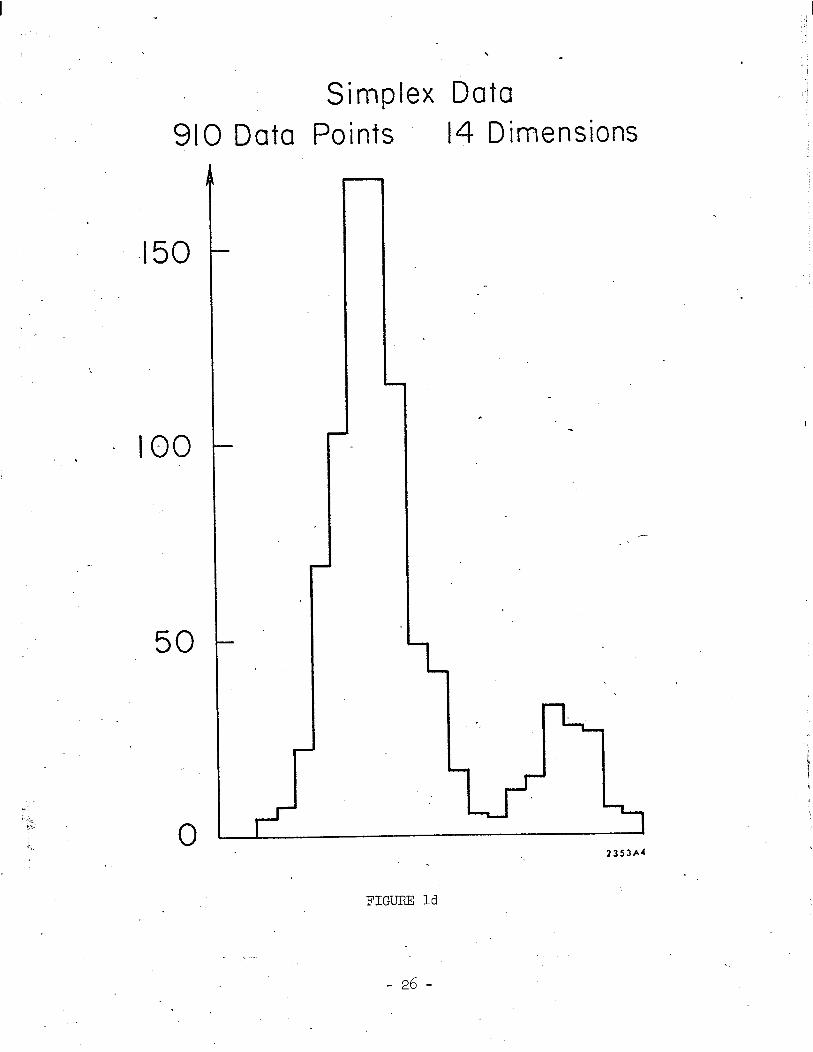
are shown in Figures lc and Id. The solution projection for the 65 point isolate 3. *.a showed no evidence for additional clustering, while the 910 point sample clearly i.
separated into two subclusters of 130 and 780 points. We further isolated these
two subclusters and applied projection pursuit to each one individually. The
results are illustrated in Figures le and l-f. The solution for the 130 point
subcluster shows it divided into two clusters of 65 points each,while the 780
point cluster separates into a 65 point cluster and 715 point cluster.
- 12 -
Continuing with these repeated applications of isolation and projection pursuit,
one finds, after using a sequence of linear projections, that the data set is
composed of 15 clusters of 65 points each.
Two-dimensional projection pursuit could equally well be applied at each
stage in the above analysis. This has the advantage that the solution at a given
stage sometimes separates the data set into three apparent clusters. The dis-
advantage is the increased computational requirements of the two-dimensional
projection pursuit algorithm.
3) Iris Data
This is a classical data set first used by Fisher 15 and subsequently by many
other researchers for testing statistical procedures. The data consists of measure-
ments made on 50 observations from each of three species,. (,one-*quite d'iffereat than
the other two) of Iris flowers. Four measurements were made on each flower and
there were 150 flowers in the entire data set. Taking the largest principal axes
as starting directions, we applied projection pursuit to the entire four-dimensional
data-+set#.:The result for two-dimensional projection pursuit is shown in Figure 2a.
As can be seen, the data as projected on the solution plane shows clear separation
into two well defined clusters of 50 (one species) and 100 (two unresolved species)
points. The one-dimensional algorithm also clearly separates the data into these
two clusters. However, this two-cluster separation is easy to achieve and is
readily apparent from simple inspection of the original data.
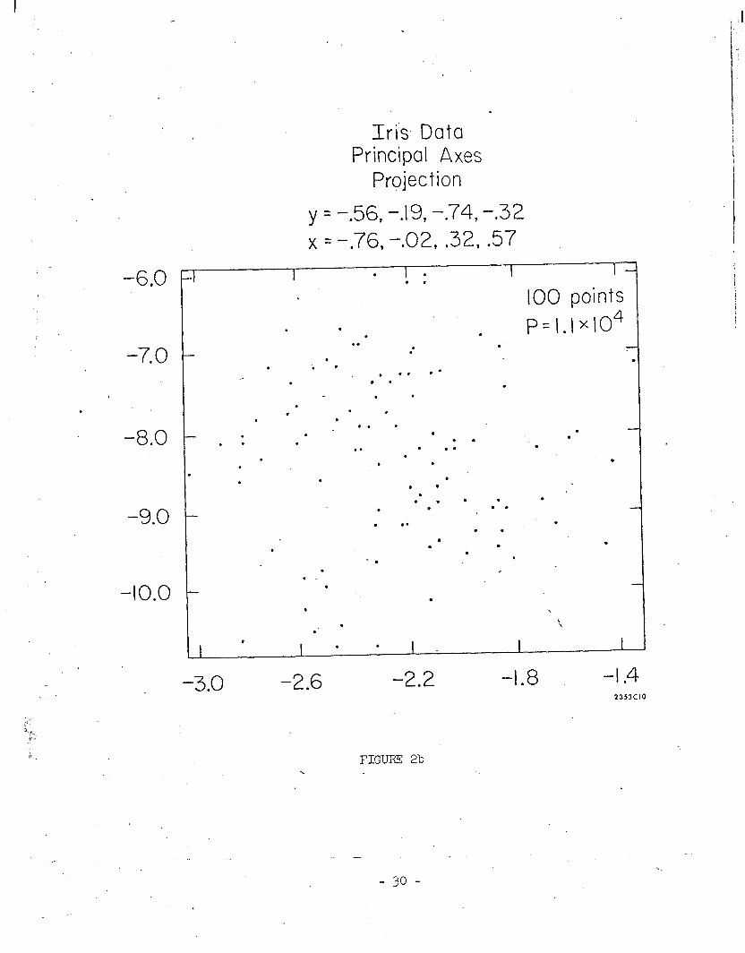
Applying the procedure discussed above, we isolate the 100 point cluster
(largest standard deviation was about six times the smallest) and re-apply pro-
jection pursuit, starting with the largest principal axes of the isolate. Figure
2b shows the data projected onto the plane defined by the two largest principal
axes. Here the data seem to show no ppparent clustering.
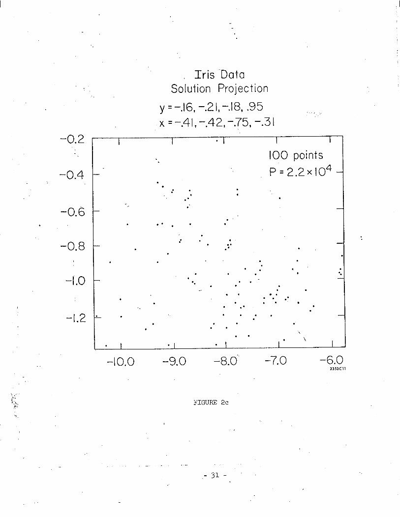
One dimensional projection pursuit, starting with the largest principal
axis, was unable to separate this isolate into d-iscerncble clusters. Figure-2c
shows the results of two-dimensional projection pursuit starting with the plane
of Figure 2b. This solution plane seems to divide the projected data into two
discernible clusters. One in the lower right hand quadrant with higher than - 13 -

average density seems slightly separated from another, which is somewhat sparser
and occupies most of the rest of the projection. In order to see to what extent
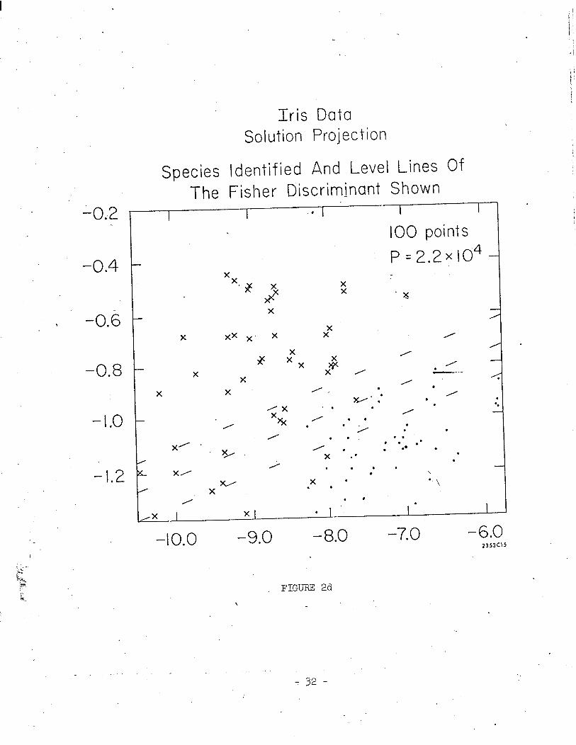
this apparent clustering corresponds to the different Iris species known to be
contained in this isolate, Figure 2d tags these species. As can be seen, the
two clusters very closely correspond to the two Iris species. Also shown in
Figure 2d are some level lines of(the projection onto the same plane of) Fisher's
linear discriminant function L3, ?, for this isolate calculated by using the known
identities of the two species. In this example, the angle between the direction
upon which this linear discriminant function is a projection, and this plane, is
a little more than 45’.
The projection pursuit solution can be compared to a two-dimensional pro-
jection of this isolate that is chosen to provide maximum separation of the two
species, given the a priori information as to which species each data:lpoint-repre-
sents. Figure 2e shows the isolate projected onto such a plane whose horizontal
coordinate is the value of Fisher's linear discriminant for the isolate in the
full four-dimensional space, ?, while the vertical axis is the value of a similar
Fisher linear discriminant in %'(?), the three-dimensional space orthogonal to
$+ . I4 (Ift.~t&dI!Wk&l;lin3 y&ria-nceJ'- were; spherica>! iAn,.-&'& ih~t&~ly~~gi~e.n- c&r&,nate
system, this vertical coordinate would not be well defined, since the centers of
the two species groups would coincide inz3(?). While we may feel that the
vertical coordinate adds little to the horizontal one, linear discrimination
seems to offer no better choice of a second coordinate, especially since we
would like this view also to be a projection of the original data -- a projection
in terms of the original coordinates and scales -- as all two-dimensional pro-
jection pursuit views are required to be.) A comparison of Figures 2d and 2e
shows that the unsupervised projection pursuit solution achieves separation Of
the two species equivalent to this discriminant plane. Since these two species
are known to touch in the full four-dimensional space, 2,4 it is probably not
possible to find a projection that completely separates them.
- 14 -

4) Particle Physics Data
For the final example, we apply projection pursuit to a data set taken from
17 a high energy particle physics scattering experiment . In this experiment, a
beam of positively charged pi mesons, with an energy of 16 billion electron volts,
was used to bombard a stationary target of protons contained in hydrogen nuclei.
Five hundred examples were recorded of those nuclear reactions in which the final
produets were a proton, two positively charged pi-mesons, and a negatively charged
pi-meson. Such a nuclear reaction with four reaction products can be completely
- described by 7 independent measurables*. This data can thus be regarded as 500
points in a seven-dimensional space.
The data projected onto its largest principal axis is shown in Figure 3a,
while the projection onto the plane defined by the largest two principal axes is
shown in Figure 3c. (The largest standard deviation was about eight times the
smallest). One-dimensional projection pursuit was applied starting with the largest
principal axis. Figure 3b shows the data projected onto the solution direction.
The result of a two-dimensional projection pursuit starting with the plane of
Figure 32 is shown in Figure 3d.
Although the principal axis projections indicate possible structure within
the data set, the projection pursuit solutions are clearly more revealing. This
is indicated by the substantial increase in the P-index, and is verified by visual
inspection. In particular, the two-dimensional solution projection shows that
there are at least three clusters, possibly connected, one of which reasonably
separates from the other two. Proceeding as above, one could isolate this cluster
from the others and apply projection pursuit to the two samples separately, con-
=: tinuing the analysis.
CQ * -I- + For this reaction, zbf pt +pzl n2 n-, the following measurables were used:
x1 = /A2(?c, 37;) ni), x2 = P2& + x3 = V2(P, 4, x4 = P2(C g> x5 = P2(P, q,
x6 = p2(??, ?(;> -p,), and X7 = P(P, fli, -P,). Here, p2(A, B, * C) = (EA f EB f EC)'
-(FA + FB 2 FC)' and y2(A, -t- B) = (EA k EB)2 - (FA 5 ?B)2, where E and? represent
the particle's energy and momentum respectively, as measured in billions of electron volts. The notation (a2-represents the inner-product ?s?. The ordinal assignment of the two n'lS was done randomly.
- 15 -

I
Discussion
The experimental results of the previous section indicate that the PP algo-
rithm behaves reasonably. That is, it tends to find structure when it exists in
the multidimensional data and it does not find structure when it is known not to
exist. When combined with isolation, projection pursuit seems to be an effective
tool for the detection of certain types of clustering.
Because projection pursuit is a linear mapping algorithm, it suffers from
some of the well known limitations of linear mapping. The algorithm will have
difficulty in detecting clustering about highly curved surfaces in the full dimen-
sionality. In particular, it cannot detect nested spherical clustering. It can,
however, detect nested cylindrical clustering where the cylinders have parallel
generators.
Projection pursuit leaves to the researcher's discretion the choice of
measurement variables and metric. The algorithm is, of course, sensitive to
change of relative scale of the input measurement variables, as well as to highly
nonlinear transformations of them. If there is no a priori motivation for a
choice of scale for the measurement variables, then they can be independently
scaled (standardized) so as to all have the same variance. In the spirit of
exploratory data analysis, the researcher might employ projection pursuit to
several carefully selected non-linear transformations of his measurement variables. -,
For example;-transformations'-to various-spherical polar coordinate:representations 11
would enable projection pursuit to detect nested spherical clustering. Frequently with multidimensional data, only a few of the measurement
variables contribute to the structure or clustering. The clusters may overlap
in many of the dimensions and separate in only a few. As pointed out by both
Sammon' and Kruskal' , those variables that are irrelevant to the structure or
clustering can dilute the effect of those that display it, especially for those
mapping algorithms that depend solely on the multidimensional interpoint distances.
It is easy to see that the projection pursuit algorithm does not suffer seriously
- 16 -

from this effect. Projection pursuit will automatically tend to avoid projections
involving those measurement variables that do not contribute to data structure,
since the inclusion of these variables will tend to reduce d(E) while not modi-
fying s(2) greatly.
In order to apply the PP algorithm, the researcher is not required to possess
a great deal of a priori knowledge concerning the structure of his data, either
for setting up the control parameters for the algorithm or.for interpreting its
results. The only control parameter requiring care is the characteristic radius
g defined in eqn. 4. Its value establishes the minimum scale of density variation
detectable by the algorithm. A choice for its value can be influenced by the
global scale of the data as well as any information that may be known about the
nature of the variations in the multivariate density of the points. The sample
size is also an important consideration since the radius should be large enough
to include, on the average, enough points (in each projection) to obtain a
reasonable estimate of the local density. These considerations usually result
in a compromise,. r=-~' making $ as small as possible, consistent with the sample
size requirement. Because of the computational efficiency of the algorithm,
however, it is possible to apply it several times with different values for I.
Interpretation of the results of projection pursuit is especially straightforward
owing to the linear nature of the mapping.
The researcher also has the choice of the dimensionality of the projection
subspace. That is, whether to employ one, two or higher dimensional projection
pursuit. The two-dimensional projection pursuit algorithm is slower and slightly
less stable than the one-dimensional algorithm; however, the resulting two-
dimensional map contains much more information about the data. Experience has
shown that a useful strategy is to first find several one-dimensional PP solutions,
then use each of these directions as one of the starting axes for two-dimensional
projection pursuits.
Acknowledgment
Helpful discussions with William H. Rogers.. and Gene H. Golub are gratefully acknowledged.
- I( -

APPENDIX
This section presents the solid angle transform (SAT) that reversibly maps
the surface of a unit sphere in an n-dimensional space, Sn(l), to an (n-l)-
dimensional infinite Euclidean space, E n-l (-%4* This transformation is de-
rived in Reference 11 and only the results are presented here.
Let (X1,X2,. ..j :X!n)be the coordinates of a point lying on the surface of an
n-dimensional unit.. sphere and (7 7 1' 2’” .?lnml) be the corresponding point in an
(n-l)-dimensional unit hypercube E n-1(0,1). Then for -n.:even, the :transformaltion
is 1 1
'2i = [.~~ n:;i(n-21)l COS [sin-1,1i{(n-2i;I sin(2fly2i-l)
(1 Ci. <n/2-1)
b-f -1 xjn = n 2-1 ,1-/b-23 -3 sin(2Jrr] )
n-l . L j=l J
X 2i-1 = '2i cot (274 2i-1)
xn =
x = n-l
x 2i =
'2i-1 =
(15i<n/2) ,
L j=l J
n-3
l/(n-2J>
i I
All
j=l 2j
(Tn-2 - 11,2_2)1’2 sin(2flVn-l)
! 5: ?)2j l/C n-2j 11
] cos [sin-1712i1/(n-2ig sin( 2nV2i-l)
1 5 i 5 (n-3)/2
X 2i cot (2l-q 2i-1) IS i s (n-1)/2 .
- la -

The Jacobian of this transformation,
Jn(l) = 2~7~ 42 > rc;,
is a constant, namely the well known expression for the surface area of an
n-dimensional sphere of unit radius. Adjusted by a factor of the (n-1)st root
of J n, the transformation is volume preserving, one to one, and onto. The in-
verse transformation can easily be obtained by solving the above equations for
the q's in terms of the X-coordinates. The unit hypercube, E n-1(0,1), can be
expanded to the infinite Euclidean space, E n-l (-co,oo), by using standard 8S.
techniques, la specifically multiple reflection.
- 19 -

REFERENCES
1. Bolshev, L.N. 1969. Bull. Internat. Stat. Inst., 3, pp 411-425.
2. Zahn, C.T., "Graph-theoretical methods for detecting and describing gestalt clusters,' IEEE Trans. Computers, Vol. C-20, pp. 68-86, January 1971.
3. Shepard, R.N. and Carroll, J.D., "Parametric representation of non- linear data structures,' in Multivariate Analysis, P. Krishnaiah, Ed., New York: Academic Press, 1966.
4. Sammon, Jr., J.W., "A nonlinear mapping for data structure analysis", IEEE Trans. Computers, Vol. C-18, pp. 401-409, May 1969.
5. Kruskal, J.B., 'Toward a practical method which helps uncover the structure of a set of multivariate observations by finding the linear transformation which optimizes a new 'index of condensation'," in Statistical Computation, R.C. Milton and J.A. Nelder, Ed., New York, Academic Press, 1969.
6. Kruskal, J.B., 'Linear transformation of multivariate data to reveal clustering," in Multidimensional Scaling: Theory and Application in the Behavorial Sciences, Vol. 1, Theory, New York and London, Seminar Press, 1972.
7. Rosenbrock, H.H., 'An automatic method for finding the greatest or least value of a function," Comp. J., Vol. 3, pp. 175-184, 1960.
a. Powell, M.J.D., "An efficient method for finding the minimum of a function of several variables without calculating derivates," Comp. J., vol. 7, pp. 955-162, 1964.
9. Maltson, R.L. and Dammann, J.E., "A technique for determining and coding subclasses in pattern recognition problems," IBM Journal, Vol. 9, pp. 294-302, July 1965.
10. Film: ‘JpR,-g” , produced by Stanford Linear Accelerator Center, Stanford, California, Bin 88 Productions, April 1973.
11. Friedman, J.H. and Steppel, S., "Non-linear constraint elimination in high dimensionality through reversible transformations," Stanford Linear Accelerator Center, Stanford, California, Report, SLAC PUB-1292, -August 1973.
. .
12. Derenzo, S., “MINl?-68 - A general minimizing routine," Lawrence Berkeley Laboratory, Berkeley, California, Group A Technical Report P-190, 1969.
13 * Brent, R.P., "Algorithms for minimization without derivatives," Englewood Cliffs, N.H.,: Prentice-Hall, 1973.
14. Golub, G.H., "Numerical methods for solving linear least squares problems," Numer. Math., vol. 7, pp. 206-216, 1965.
- 20 -

15.. Fisher, R.A., "Multiple measurements in taxonomic problems," Contri- butions to Mathematical Statistics, New York: Wiley.
16. Sammon, Jr., J.W., "An optimal discriminant plane," IEEE Trans. Com- puters, vol. C-19, pp. 826-829, September 1970.
17. Ballam, J., Chadwick, G.B., Guiragossian, Z.C.G., Johnson, W.B., Leith, D.W.G.S. and Moriyasu+ II., llVan Hove analysis of the reactions ~-p+~?-G-n+p and n p+fl(+n+fl p at 16 GeV/C, Phys. Rev., 2 vol, 4, pp. 1946-1947, Oct. 1971.
18. Box, M.J., Computer Journal 9, x.-67-77, (1966).
- 21 -

SPHERICALLY RANDOM DATA
14 Dimensions 975 Data Points
Search No.
P-Index Starting
P-Index Search P-Index P-Index Solution No. Starting Solution
5 6
7 a
9 10
11 12
13 14
151.8 156.3 15 150.6
150.7 156.7 16 150.6
149.4 156.0 17 151.0
152.4 159.7 18 152.2
152.3 159.2 19 152.1
151.0 154.4 20 152-P
152.6 155.6 21 150.0
149.6 155.4 22 150.0
150.0 156.1 23 150.7
151.8 153.0 24 151.5 154.0 154.6 25 151.0
151.4 156.7 26 152.8
149.7 154.1 27 151 .a
152.1 154.2 28 152.1
155.8
156.9
157.0
155-6 160.2
159-o 160.8
157-P
155.4 158.4
155.3 1.59.6 157.0
157-P
TABLE 1
- 22 -

I
. --
975
100
80
60
40
20
0
-
S mplex Data Data Points 14 Dimensions
Largest Principal Axis P-Index= 1.00 X IO5
2353Al
FIGURE 1;
-
- 23 - _ . .
Simplex Data 975 Data Points 14 Dimensions
200
P-Index=3.37x10⁵-
235382
FIGURE 1-b
- 24 -

.
.
65 Data 2op .
lot
0- 2353+
Simplex
Points _
Data 14 Dimensions
FIGURE lc
:
-25- _
Simplex Ddta 910 Data Points I4 Dimensions
.I 50
IO0
50
0 rJ
.
235344
FIGURE Id
.-
- 26 -

40
20
0
130 Data
Simplex Data 14 Dimensions
L
.
2 353~5
FIkN3 le
- .27 -

I
Simplex’ Dota
780 Data Points I4 Dimensions
,2353A6
FIGURE If
- 28 --
I

.
: 4.0
3.0
Solution Projectibn
y = 0, .04, .83, ~56 - X = -.16, .23, -.54, -.79
. I I I I .‘ I . . .
l . . I50 points . .
. . .
.*. . .* .*.
. . .* . . l . .
c
. . l l _.* l . l . . . . l . . 0.0
. . .* ,* .*
.* . ‘==: . . .* . .
. .*
. 0.
. . .
l .* l . . .
2.0
-6.0 -5.0 -4.0
l
. .
.* .*.:*. . . . l .:c .* . l y.7”. .*.
. l . . .
-3.0 -2.0 -1.0 2353C9
FIGURF: 2a
- 29 -
Iris Data
-6.0
-7.0
,
-8.0
-9.0
-10.0
Principal Axes Project ion
Y = -.56, -.19, ~74, -.32 X= -76, -.02, .32, .57
- 1 I I - . . . .
. .
100 points . P=l.lx104 .
. . : :
. . ‘. l
. -0 l =
, . . .
.
. .
. .
. .
. .
. . l
. . . .
. . .
.
. l .
l . . . . .
. . . .
.
. .
.
. . . .
. . l
.
. . l . .
. . . .
. . . . . .
. . . . .
.
.
I
.
. I I . . I I I
-3.0 -2.6 -2.2 -1.8 -1.4 2353ClO
FIGURE 2b
I_
- 30 -
, Iris ‘Data Solution Projection
Y = -.16, -21, -.18, .95
-0.2
-0.8
,X = -.4l, -.42, -.75, -.3 I
. .
:
. l .
.
. .*’ :
. l
.* . .
100 points P=2.2x10⁴
.
. .
. . .
. - -1’ .
. . .
. .
. . . .
l : .
. . *
. . . . . .
. . . . . . .* . . l .
. .* .
.
. . . . .
. :
.
. . I
-10.0 -9.0 -8.0’. -7.0 -6.0 2353Cll
FIGUFiE 2c
_ _._.. - _ - .-31.7
. -0.G
-0.8
Iris Data Solution Projection
Species Identified And Level Lines Of The Fisher Discriminant Shown
I I . I I 100 points P=2.2x10⁴
I
I L----
. / .
.
.
X
X
xx *
xx x
x X
>E2( X
* Y
X
0 . . . . . . . .- 0 .
x .* l
.* . .
i
.
. . l .
. ‘\
x l ‘\ . .
. * .
-10.0 -9.0 -8.0 -7.0 -6.0 2353Clf,
FIGURE 2d
I
/
.
. l .

2.5
I.5
Iri.& Data _ Linear Discriminant
Projection
X = -.80, -.05, -.09, -.60 y=.60, .06, -.09, -.80
I . I I
. . l . . .
. .
X l .
x x
X l . l .
X . . . . . . ,
‘. .
K
X
X X
. X
x- x X
xx
X X
X ‘. . .
. .
i< xx
. X x l * . .
X . . . . . xx l x
. *
xx
.
xxx l
x x .
X
.
X . .
X
X X X
X
I X I I
7.0 6.0 . .
FIGURE 2e
- 33 -
5.0 2353C12

40
20
0
Particle Physics +-P -7f -I- 4- p-r -7-C . .
Data 16 GN..c
Largest Principa! Axis. P-Index = 2630
,
I I I I I . I I
-15 ‘-IO -5 0 5 IO I5 2353A7
FIGURE 3a
-34-

t
120
Particle Physics Data 77-+p--+- -TT+~T+TT- I6 GeVk
100
- 80
60
40
20
Solution Projection P-Index= 5879 -
.
,I I I I I 0 1
-20 -15 -10 -5 2353A8
3*
FIG% 3b
- 35 -

Particle Physics Data
15‘
IO
. 5,
0
-5
-10
-15
lT+p - -rfp-r’-r- 16 GeWc Largest Principal Axes
Projection P-Index = 45.3
I I I I I . . . - . .@.... . . . . . 0.0 . . . . . .
. .
.
. :.. . . . . . . . . . . . z l l
.t l
.* * . . l l 0. . : .
. , . \ . . .
. . . .
. . .
. . : l 0’.
. % l
. . . . .* . . . .
c l .
. l .:...
. : ’ . . .
. ’ ’ . l
. . . . :. . . l : .:*.. . .’ . ..- . . .
. . . ., .: .
. . . . . . .., l
. . . . ’ . l .:.* . . . .
l .- . . .
. . . . l , *
. . . :’ . . .* * 2 . . . . .
. l l ‘. . . . .
. l l l .* . . . . . . : . .
* . : . 0. l ‘.*.
. . 2 l . . .: . , . . . . .
. ,.,I. . . i .-•
. . * . . . ‘.
l .
’ l . . . . . 0.. l . . l . . . . . l
l . . . . . . . .
. . l l .
. l . . . .; l
I I I I I l .*
-20 45 -10 -5 0 5 2353c,3
FIGURE 3c
- 36 -

.
0
.
-5
I Particle Physics Data 7T+p- 77-+p~‘7~ 16 GeV/c
Solution Projection P-Index = 305.0
. .
*. . l 2 . .
. l ; . . ,.. .* . . . -. . .
. .
. O.’ t l . .
l :*’ l * . . .,. . . . . :
. . : -. . . . . . . . . . . .
. l .*
* ‘. .
. , . 2 . ‘ .
.*
. . .
l . .** l ,
.* . .* l . . . . . l .
*. * . l 0
. . .
Z7.Y . = .y4*. .
..*,. . . ‘..*‘, . 5 ‘. l *?&<. .
l . . . : .
l . ..*
. . .
.
.
. .
\ .
I I . I I I
I.
2 ,. I\ .
. . i
. . l .
a . ..*
.’
-15 -IO -5 0 5 IO I5 2353Cl4
.
FIGURE 3d
._ -.37 -