(m)-Self-Dual Polygons

THESIS

Submitted in Partial Fulfillmentof the Requirements for the

Degree of

BACHELOR OF SCIENCE (Mathematics)

at the

POLYTECHNIC INSTITUTE OF NEW YORK

UNIVERSITYby

Valentin Zakharevich

June 2010

(m)-Self-Dual Polygons

THESIS

Submitted in Partial Fulfillment

of the Requirements for the

Degree of

BACHELOR OF SCIENCE (Mathematics)

at the

POLYTECHNIC INSTITUTE OF NEW YORK UNIVERSITY

by

Valentin Zakharevich

June 2010

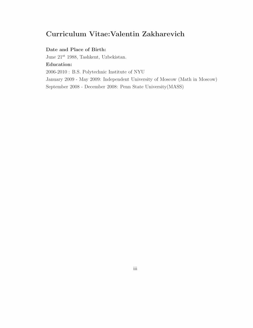
Curriculum Vitae:Valentin Zakharevich

Date and Place of Birth:

June 21st 1988, Tashkent, Uzbekistan.

Education:

2006-2010 : B.S. Polytechnic Institute of NYU

January 2009 - May 2009: Independent University of Moscow (Math in Moscow)

September 2008 - December 2008: Penn State University(MASS)

iii

ABSTRACT

(m)-Self-Dual Polygons

by

Valentin Zakharevich

Advisor: Sergei Tabachnikov

Advisor: Franziska Berger

Submitted in Partial Fulfillment of the Requirements

for the Degree of Bachelor of Science (Mathematics)

June 2010

Given a polygon P = {A0, A1, . . . , An−1} with n vertices in the projective space

CP2, we consider the polygon Tm(P ) in the dual space CP∗2 whose vertices correspond

to the m-diagonals of P , i.e., the diagonals of the form [Ai, Ai+m]. This is a general-

ization of the classical notion of dual polygons where m is taken to be 1. We ask the

question, ”When is P projectively equivalent to Tm(P )?” and characterize all poly-

gons having this self-dual property. Further, we give an explicit construction for all

polygons P which are projectively equivalent to Tm(P ) and calculate the dimension

of the space of such self-dual polygons.

iv

Contents

1 Introduction 1

2 Projective Geometry 3

2.1 Projective Spaces . . . . . . . . . . . . . . . . . . . . . . . . . . . . . 3

2.2 Coordinates . . . . . . . . . . . . . . . . . . . . . . . . . . . . . . . . 4

2.3 Projective Isomorphisms . . . . . . . . . . . . . . . . . . . . . . . . . 7

2.4 Cross-Ratio . . . . . . . . . . . . . . . . . . . . . . . . . . . . . . . . 9

2.5 Projective Duality . . . . . . . . . . . . . . . . . . . . . . . . . . . . 12

2.6 Bilinear Forms . . . . . . . . . . . . . . . . . . . . . . . . . . . . . . 15

2.6.1 Symmetric Bilinear Forms . . . . . . . . . . . . . . . . . . . . 16

2.6.2 Non-symmetric Bilinear Forms . . . . . . . . . . . . . . . . . . 20

3 (l, m)-Self-Dual Polygons 27

3.1 Notation . . . . . . . . . . . . . . . . . . . . . . . . . . . . . . . . . . 28

3.2 The Case n = 2l + m . . . . . . . . . . . . . . . . . . . . . . . . . . . 28

3.2.1 Explicit Construction . . . . . . . . . . . . . . . . . . . . . . . 31

3.3 The Case n 6= 2l + m . . . . . . . . . . . . . . . . . . . . . . . . . . . 33

3.3.1 Explicit Construction. . . . . . . . . . . . . . . . . . . . . . . 34

4 Geometric Surprises 40

4.1 Corner Invariants . . . . . . . . . . . . . . . . . . . . . . . . . . . . . 42

4.2 Geometrical Proofs . . . . . . . . . . . . . . . . . . . . . . . . . . . . 44

4.2.1 Inscribed 6-gons. . . . . . . . . . . . . . . . . . . . . . . . . . 45

4.2.2 Inscribed 7-gons. . . . . . . . . . . . . . . . . . . . . . . . . . 49

5 Conclusion 52

v

1 Introduction

The field of projective geometry originated as a study of geometrical objects under

projections which was particularly important in fine art and architecture. In order

to create an image that has the correct perspective, one needs to know how three-

dimensional objects project onto two-dimensional canvas. In modern times, one may

find applications of projective geometry in 3D graphics and computer vision.

An important object in this area is the space of lines passing through a given

point. Let a point p be fixed in a three dimensional space, and let a plane L be given

which does not intersect the point p. We can associate points on the plane L with

lines passing through the point p by drawing a line through that point on the plane

and p. This covers almost all lines passing through p except for the lines which are

parallel to L. For that reason, regular Euclidean planes are not ideal objects to study

projections. The ideal object of study is the set of lines passing through the point p.

This object, the projective plane, is a plane with additional structure at “infinity”.

For a more thorough introduction to the field, see [1].

Although the study of projective geometry originates from purely geometric in-

centives, it possesses a rich algebraic structure. For example, projective spaces are

ideal for studying algebraic curves. Also, there are interesting geometric relations

in projective spaces that arise from algebraic constructions. In this thesis, we will

closely work with the dual projective space which arises from the notion of dual vector

spaces.

It turns out that the most natural way to define and study projective spaces is

by considering vector spaces. We will assume that the reader is familiar with vector

spaces and will not define notions or prove statements that one should learn in a

standard Linear Algebra course.

In Section 2 of this thesis we will introduce the notion of projective geometry

and projective duality which will serve as the foundation for the work presented in

Section 3.

In Section 3 we will present original research that has originated

from the work done during an REU(Research Experience for Undergraduates)

1

program at the Penn State University during the summer of 2009. Given an n-gon

P = {A0, A1, . . . , An−1} in the projective plane, we will consider the n-gon Tm(P )

in the dual projective plane whose vertices correspond to m-diagonals of P i.e., the

diagonals of the form [Ai, Ai+m]. We will construct all n-gons P with the property

that P is projectively equivalent to Tm(P ) and calculate the dimension of the space

of such m-self-dual polygons.

In Section 4 we will present the recently discovered relations between m-self-dual

n-gons and those n-gons inscribed into a non-singular conic. These relations are still

not very well understood and have partially motivated the research of Section 3.

2

2 Projective Geometry

2.1 Projective Spaces

Let V be an n-dimensional vector space over a field k. The n-dimensional affine

space An = A(V ) is the geometric representation of V . The points of An correspond

to vectors of V , and the origin corresponds to the zero vector. The n-dimensional

hyperplanes of An are translations of n-dimensional subspaces of V . The definition of

affine spaces provides a natural dictionary between the language of algebra and the

language of geometry.

Let V be an (n + 1)-dimensional vector space over a field k. Let Pn = P(V ) be

the projectivization of the vector space V : the points of P(V ) are one-dimensional

subspaces of V or, equivalently, lines passing through the origin in A(V ). To visualize

the points of the projective space, one uses a screen, i.e., an n-dimensional hyperplane

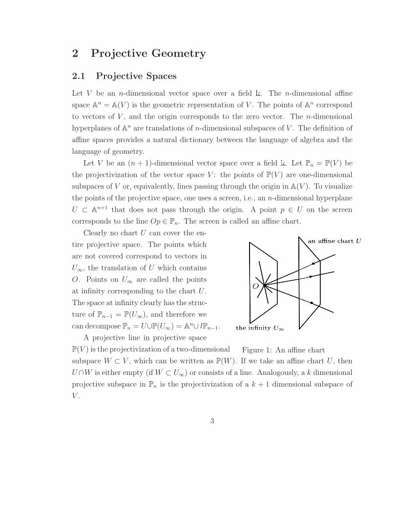
U ⊂ An+1 that does not pass through the origin. A point p ∈ U on the screen

corresponds to the line Op ∈ Pn. The screen is called an affine chart.

Clearly no chart U can cover the en-

Figure 1: An affine chart

tire projective space. The points which

are not covered correspond to vectors in

U∞, the translation of U which contains

O. Points on U∞ are called the points

at infinity corresponding to the chart U .

The space at infinity clearly has the struc-

ture of Pn−1 = P(U∞), and therefore we

can decompose Pn = U∪P(U∞) = An∪ lPn−1.

A projective line in projective space

P(V ) is the projectivization of a two-dimensional

subspace W ⊂ V , which can be written as P(W ). If we take an affine chart U , then

U∩W is either empty (if W ⊂ U∞) or consists of a line. Analogously, a k dimensional

projective subspace in Pn is the projectivization of a k + 1 dimensional subspace of

V .

3

Proposition 2.1. Let U, W be two projective subspaces of Pn such that

dim U + dim W ≥ n, then U ∩W 6= ∅.

Proof. Let U ′, W ′ ⊂ V be such that P(U ′) = U and P(W ′) = W . Then

dim U ′ = dim U + 1,

dim W ′ = dim W + 1,

and

dim U ′ + dim W ′ ≥ n + 2.

Since dim V = n + 1, U ′ ∩W ′ 6= {0}, or equivalently, U ∩W 6= ∅

In particular, this means that any two lines in P2 intersect.

2.2 Coordinates

Let V be an n+1-dimensional vector space over k and let {e0, e1, ..., en} be a fixed basis

of V . Any two vectors v = {v0, v1, . . . , vn} and w = {w0, w1, . . . , wn}, represented in

terms of the fixed basis, represent the same point p ∈ P(V ) if and only if vi = λwi

for some λ 6= 0. Therefore only the ratios vi

vjare necessary to represent a point p.

Thus we write p = (v0 : v1 : . . . : vn) (defined up to proportionality) for the point

represented by the vector v = {v0, v1, . . . , vn}.

We would also like to know how to introduce a coordinate system on an affine

chart. Let U be an affine chart. There exists a unique α ∈ V ∗, where V ∗ is the vector

space dual to V consisting of all linear maps V → k, such that U is given by the

equation α(x) = 1 1. We will denote this affine chart by Uα. Let v ∈ V be such that

α(v) 6= 0. The one dimensional subspace spanned by v intersects U at the point vα(v)

.

Otherwise, if α(v) = 0 then v ∈ U∞. To introduce coordinates on the affine chart

Uα, fix n linear forms x1, x2, ..., xn ∈ V ∗, such that along with α, they form a basis

1This is the case since a hyperplane of codimension 1 in An+1 is given by the equation∑n

i=0αixi = β . It passes through the origin if and only if β = 0. Therefore, since an affine chart

is a hyperplane that does not pass through the origin, we can write it as α(x) =∑n

i=0

αi

βxi = 1

4

for V ∗. To any point p ∈ Uα which is represented by a vector v ∈ V , we can assign

n coordinates ti = xi(v

α(v)). Clearly these numbers do not depend on the choice of

the vector v, since they are the same for λv, where λ 6= 0. Now given these affine

coordinates (t1, t2, . . . , tn) of a point p ∈ Uα, we can recover the point in the following

way. Let ei be a basis of V such that

xi(ej) = δij , i, j = 0, . . . , n

where we take x0 = α. Now it is clear to see that the point p corresponds to the

vector v = e0 +n∑

i=1

tiei.

Example 2.2. Let P2 = P(V ), {e0, e1, e2} be a fixed basis of V and {x0, x1, x2} the

corresponding dual basis such that xi(ej) = δij for i, j = 0, 1, 2. A polynomial q in the

variables xi does not give a well defined function on Pn, since in general q(v) 6= q(λv),

but if q is homogeneous of degree d then λdq(v) = q(λv), and the set q(v) = 0 is a

well defined set in Pn. Consider the following homogeneous equation.

x20 + x2

1 = x22

This is the equation of a cone in A3 if we are working over the field R, and we

will see how it looks like in different affine charts of P. (Of course we expect to get

different conic sections.)

Consider the affine chart Ux2 . Let our coordinates on this chart be t0, t1 where

t0 = x0(v

x2(v)) and t1 = x1(

vx2(v)

). A point p with coordinates (t0, t1) corresponds to

the vector t0e0 + t1e1 + e2, and equivalently the equation of the cone restricted to Ux2

becomes

t20 + t21 = 1

which is a circle. Analogously if we consider Ux0, t1 = x1|Ux0and t2 = x2|Ux0

, then

the equation becomes

1 + t21 = t22

5

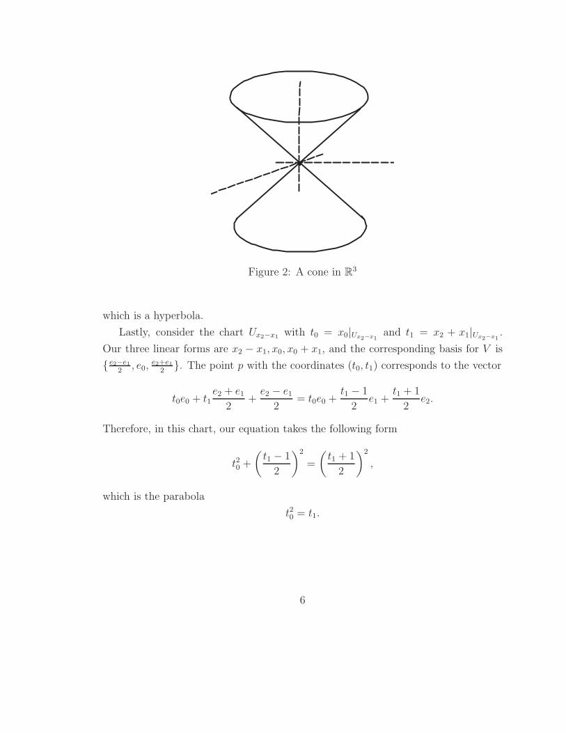
Figure 2: A cone in R3

which is a hyperbola.

Lastly, consider the chart Ux2−x1 with t0 = x0|Ux2−x1and t1 = x2 + x1|Ux2−x1

.

Our three linear forms are x2 − x1, x0, x0 + x1, and the corresponding basis for V is

{ e2−e1

2, e0,

e2+e1

2}. The point p with the coordinates (t0, t1) corresponds to the vector

t0e0 + t1e2 + e1

2+

e2 − e1

2= t0e0 +

t1 − 1

2e1 +

t1 + 1

2e2.

Therefore, in this chart, our equation takes the following form

t20 +

(

t1 − 1

2

)2

=

(

t1 + 1

2

)2

,

which is the parabola

t20 = t1.

6

2.3 Projective Isomorphisms

When studying a particular space, it is natural to consider isomorphisms which pre-

serve important properties of this space. In our case the natural isomorphism is a

projective linear isomorphism. Let U , V be two (n + 1)-dimensional vector spaces.

A vector linear isomorphism f : U → V induces a map f : P(U) → P(V ) which is

called a projective linear isomorphism. f takes the point p corresponding to vector

v to the point f(p) corresponding to the vector f(v). It is clear that the map f

is well defined, and that two linear isomorphisms f, g from U to V give rise to the

same projective linear isomorphism if and only if they are proportional. The map f

sends k-dimensional hyperplanes to k-dimensional hyperplanes the same way f takes

(k + 1)-dimensional subspaces to (k + 1)-dimensional subspaces. To justify the term

“projective”, consider the following example.

Proposition 2.3. Let l1, l2 be two lines in P2, and let p /∈ l1 ∪ l2. If the map

πp : l1 → l2 is the projection that sends a point q ∈ l1 to the intersection of lines

[q, p] ∩ l2, then it is a projective linear isomorphism.

Figure 3: Projection in P2

Proof. Let e0 ∈ V represent l1 ∩ l2. Pick any point q ∈ l1 not equal to l1 ∩ l2.

Let e1, e2 ∈ V be such that e1 represents q, e2 represents πp(q), and e1 + e2 repre-

7

sents p. This can clearly be done since we can scale e1, e2 and p lies in the span

of {e1, e2}. Now if we let {e0, e1} be the basis of the subspace corresponding to l1

and {e0, e2} be the basis of the subspace corresponding to l2, the map πp is induced

from the map M , which sends e0 → −e0 and e1 → e2.2 To see this, take a point r

corresponding to xe0 + ye1 where y 6= 0 and consider the point r′ corresponding to

M(xe0 + ye1) = −xe0 + ye2. Now it is clear that πp(r) = r′ since p = e1 + e2 lies in

the span of {xe0 + ye1,−xe0 + ye2}. If r corresponds to e0, then it is clearly fixed by

both πp and M .

Definition 1. A set of points {p1, p2, . . . , pm} ⊂ Pn = P(V ) is called linearly general

if no collection of (n + 1) points pi lies on a hyperplane Pn−1 ⊂ Pn.

Equivalently, this means that for any collection of (n + 1) points pi, the set of

vectors representing those points forms a basis for V .

Proposition 2.4. Let dim(U) = dim(V ) = (n+1) and let {p0, p1, . . . , pn+1} ⊂ P(U),

{q0, q1, . . . , qn+1} ⊂ P(V ) be two linearly general collections of points. Then there

exists a unique projective linear isomorphism M : P(U)→ P(V ) such that M(pi) = qi

for all i.

Proof. Fix vectors pi ∈ U and qi ∈ V such that pi and qi represent points pi and qi re-

spectively for all i. Since both collections of points are linearly general, {p0, p1, . . . , pn}

and {q0, q1, . . . , qn} form basis for U and V , respectively. If a linear map M : V → U

induces a desired map M : P(U)→ P(V ) then M(pi) = λiqi for some non-zero num-

bers λi and i = 0, 1, . . . , n. Also, since {p0, p1, . . . , pn} and {q0, q1, . . . , qn} are bases

for U and V respectively and since the two collections of points are linearly general,

there are unique non-zero constants ai and bi such that

pn+1 =n∑

i=0

aipi qn+1 =n∑

i=0

biqi

2With respect to the given basis, the map M has the following matrix,

(

−1 00 1

)

and therefore

is clearly non-degenerate.

8

The numbers ai are not zero for all i since otherwise pn+1 would belong to some

hyperplane Pn−1 ⊂ Pn spanned by n points pi contradicting that the collection

{p0, p1, . . . , pn+1} is linearly general. Similarly, the numbers bi are not zero for all i .

Also

M(pn+1) =

n∑

i=0

λiaiqi

and M(pn+1) = qn+1 if and only if λi = c bi

aifor some non zero constant c and all i.

These numbers are well defined since ai 6= 0. The map M induces the same projective

isomorphism M for any value of c which is therefore defined uniquely.

For example this means that any three points on P1 can be sent to any other three

points on P1 via a projective linear isomorphism, and there is a unique such map.

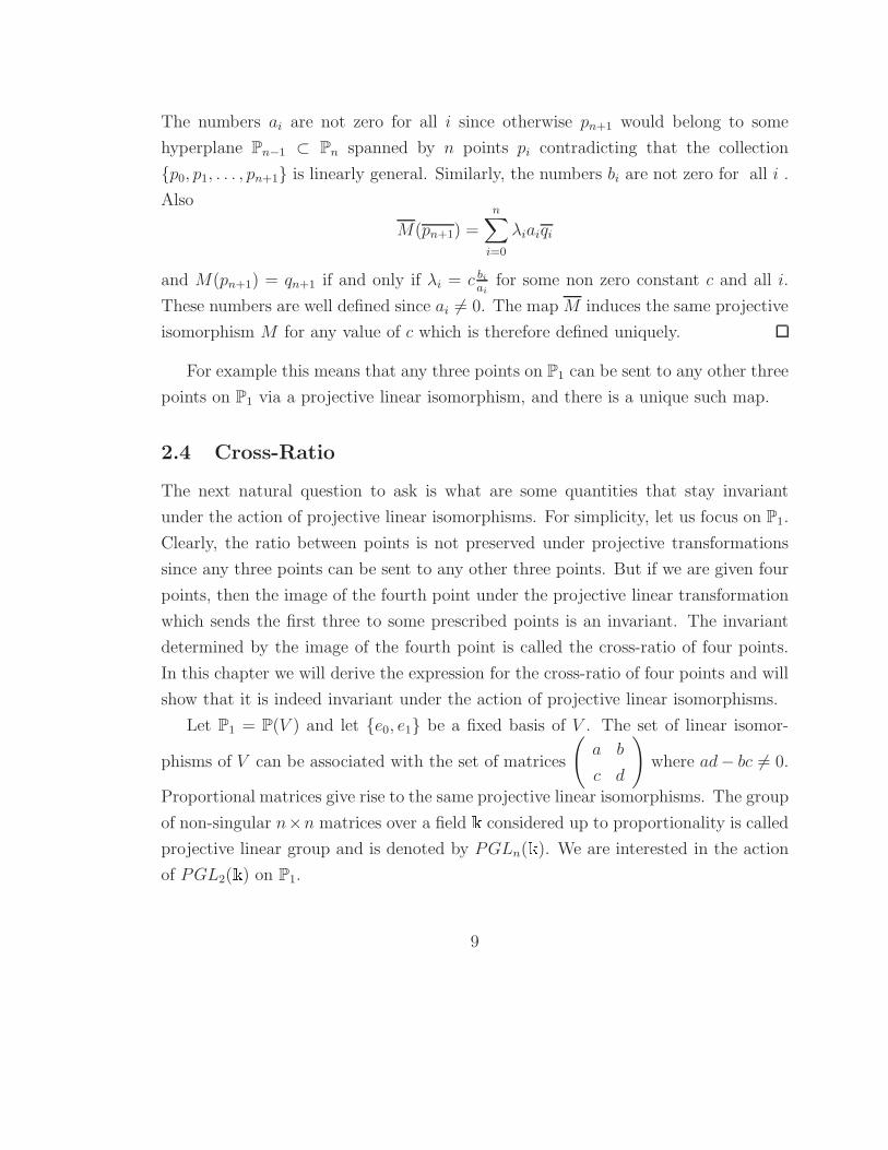
2.4 Cross-Ratio

The next natural question to ask is what are some quantities that stay invariant

under the action of projective linear isomorphisms. For simplicity, let us focus on P1.

Clearly, the ratio between points is not preserved under projective transformations

since any three points can be sent to any other three points. But if we are given four

points, then the image of the fourth point under the projective linear transformation

which sends the first three to some prescribed points is an invariant. The invariant

determined by the image of the fourth point is called the cross-ratio of four points.

In this chapter we will derive the expression for the cross-ratio of four points and will

show that it is indeed invariant under the action of projective linear isomorphisms.

Let P1 = P(V ) and let {e0, e1} be a fixed basis of V . The set of linear isomor-

phisms of V can be associated with the set of matrices

(

a b

c d

)

where ad− bc 6= 0.

Proportional matrices give rise to the same projective linear isomorphisms. The group

of non-singular n×n matrices over a field k considered up to proportionality is called

projective linear group and is denoted by PGLn(k). We are interested in the action

of PGL2(k) on P1.

9

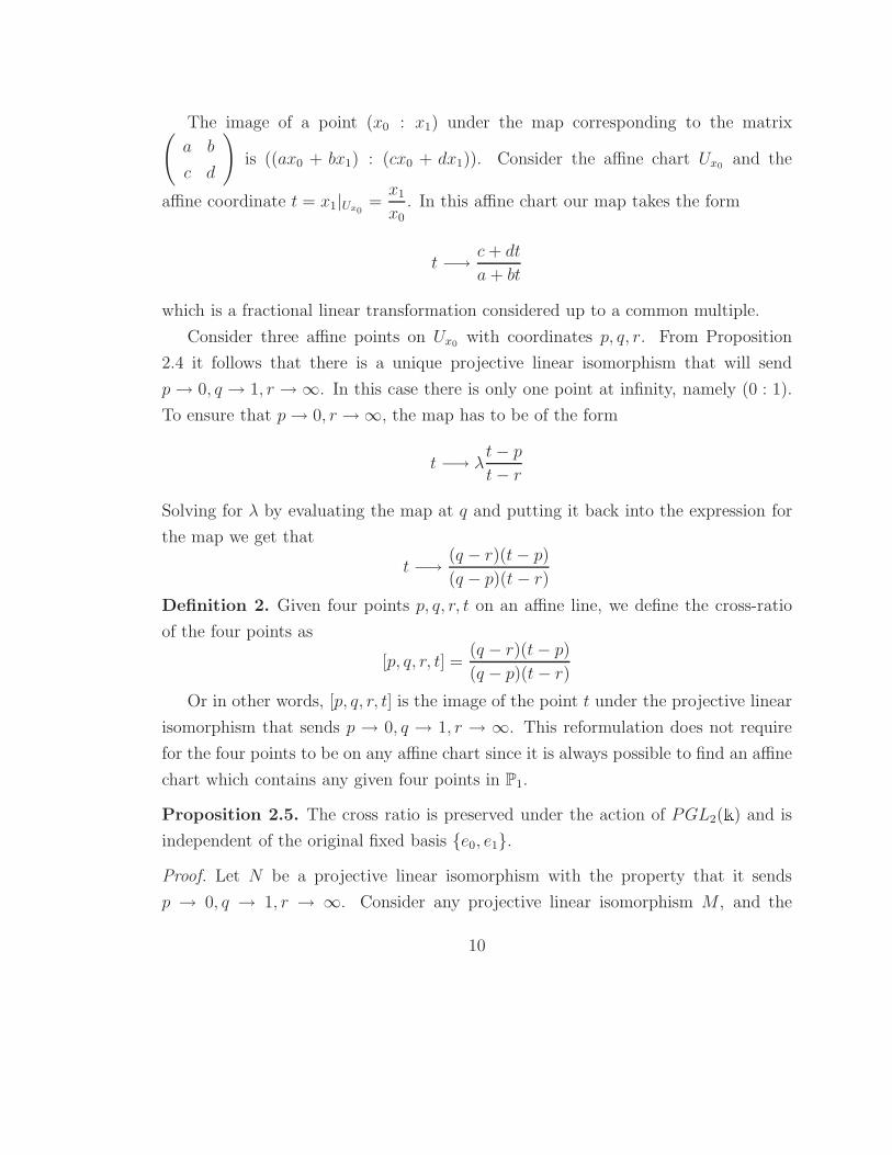
The image of a point (x0 : x1) under the map corresponding to the matrix(

a b

c d

)

is ((ax0 + bx1) : (cx0 + dx1)). Consider the affine chart Ux0 and the

affine coordinate t = x1|Ux0=

x1

x0. In this affine chart our map takes the form

t −→c + dt

a + bt

which is a fractional linear transformation considered up to a common multiple.

Consider three affine points on Ux0 with coordinates p, q, r. From Proposition

2.4 it follows that there is a unique projective linear isomorphism that will send

p→ 0, q → 1, r →∞. In this case there is only one point at infinity, namely (0 : 1).

To ensure that p→ 0, r →∞, the map has to be of the form

t −→ λt− p

t− r

Solving for λ by evaluating the map at q and putting it back into the expression for

the map we get that

t −→(q − r)(t− p)

(q − p)(t− r)

Definition 2. Given four points p, q, r, t on an affine line, we define the cross-ratio

of the four points as

[p, q, r, t] =(q − r)(t− p)

(q − p)(t− r)

Or in other words, [p, q, r, t] is the image of the point t under the projective linear

isomorphism that sends p → 0, q → 1, r → ∞. This reformulation does not require

for the four points to be on any affine chart since it is always possible to find an affine

chart which contains any given four points in P1.

Proposition 2.5. The cross ratio is preserved under the action of PGL2(k) and is

independent of the original fixed basis {e0, e1}.

Proof. Let N be a projective linear isomorphism with the property that it sends

p → 0, q → 1, r → ∞. Consider any projective linear isomorphism M , and the

10

images of p, q, r, t under M . By Proposition 2.4 there exists a unique projective linear

isomorphism which sends M(p)→ 0, M(q)→ 1, M(r)→∞. But NM−1 is this map,

and therefore NM−1(M(t)) = N(t). It is clear that the cross ratio is independent of

the choice of the basis vectors since a change of basis is nothing but an application

of a linear isomorphism which we have shown to not effect the cross ratio.

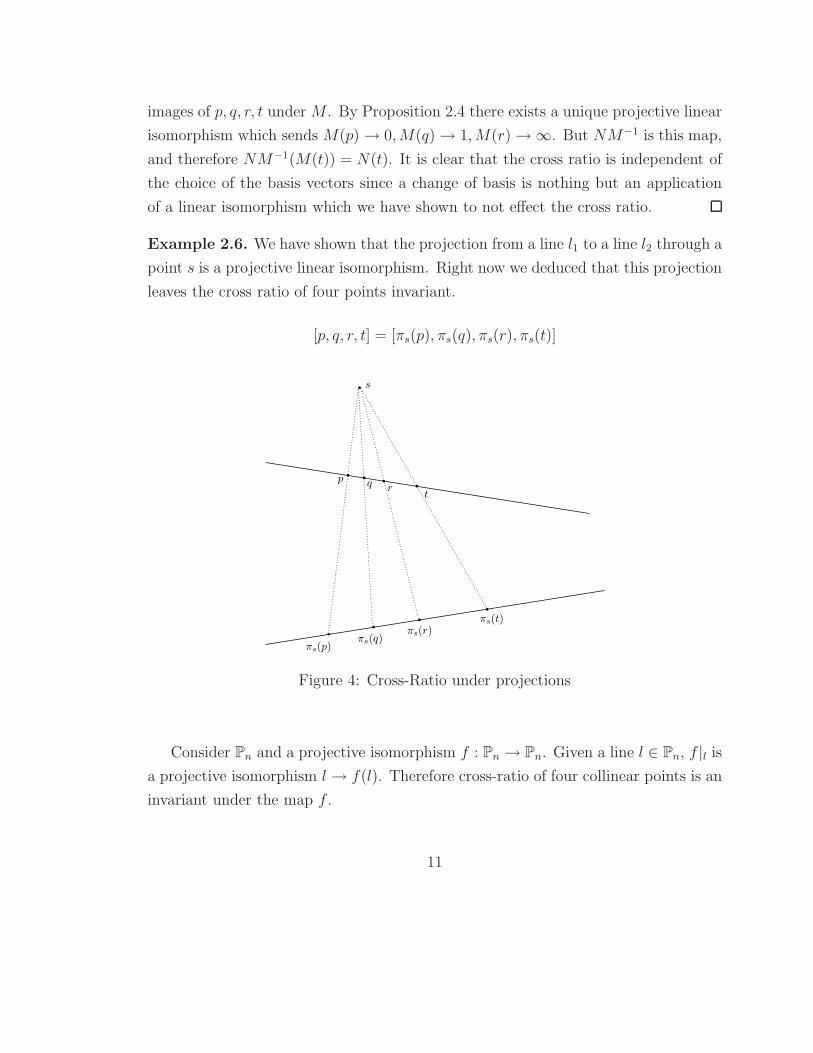
Example 2.6. We have shown that the projection from a line l1 to a line l2 through a

point s is a projective linear isomorphism. Right now we deduced that this projection

leaves the cross ratio of four points invariant.

[p, q, r, t] = [πs(p), πs(q), πs(r), πs(t)]

Figure 4: Cross-Ratio under projections

Consider Pn and a projective isomorphism f : Pn → Pn. Given a line l ∈ Pn, f |l is

a projective isomorphism l → f(l). Therefore cross-ratio of four collinear points is an

invariant under the map f .

11

2.5 Projective Duality

Let V be a finite-dimensional vector space and let V ∗ be the vector space dual to V

consisting of all linear maps α : V → k. If α ∈ V ∗ and v ∈ V , we will denote by

〈α, v〉 the value of α at v: α(v).

Definition 3. Let U be a subspace of V . Let the annihilator of U be U◦ ⊂ V ∗ where

U◦ = {α ∈ V ∗|〈α, v〉 = 0 for all v ∈ U}.

It is an elementary fact from Algebra that dim U + dim U◦ = dim V = dim V ∗.

Also, (U◦)◦ = U under the natural identification of V with (V ∗)∗. This notion of

duality becomes very important when we consider the projectivization of V and V ∗.

Definition 4. Let V be a vector space, P = P(V ) and U be a subspace of V . Define

the dual projective space as

P∗ = P(V ∗).

and the dual of P(U) ⊂ P as

P(U)∗ = P(U◦) ⊂ P∗.

Clearly (P(U)∗)∗ = P(U) for the reason that (U◦)◦ = U . The algebraic properties

of U◦ become geometric properties when we consider the duality in the projective

space.

Proposition 2.7. Let H ⊂ Pn be a hyperplane of dimension k. Then H∗ ⊂ P∗n is a

hyperplane of dimension n− k − 1.

Proof. If H is a hyperplane of dimension k, then H = P(U), where U ⊂ V is of

dimension (k + 1). By definition,

H∗ = P(U◦)

12

Since dim V = (n + 1) and dim U◦ = (n + 1)− (k + 1) = (n− k),

dim H∗ = dim U◦ − 1 = n− k − 1

For the remainder of the section we will deal with properties of duality in P2. On a

projective plane, duality takes lines to points and points to lines. What is important

is that projective duality preserves incidences in the following way

a line l ⊂ P2 ←→ a point l∗ ∈ P∗2

the points p ∈ l ←→ the lines p∗ passing through l∗

the line passing through ←→ the intersection point of lines p∗1, p∗2

two points p1, p2 ∈ P2

Proposition 2.8. Let point p be on a line l ⊂ P2. Then l∗ ∈ p∗.

Proof. Let {e0, e1, e2} be a basis of V such that e0 represents p and the linear span

of {e0, e1} represents l. Also, let {x0, x1, x2} be the basis of V ∗ such that

〈xi, ej〉 = δij

It follows that x2 represents l∗ and that the linear span of {x1, x2} represents p∗.

Therefore l∗ ∈ p∗.

Proposition 2.9. Let p1, p2 ∈ P2, and let l be the line passing through p1 and p2.

Then p∗1 and p∗2 intersect at l∗.

Proof. By Proposition 2.8, l∗ ∈ p∗1 and l∗ ∈ p∗2, which means exactly that p∗1 and p∗2intersect at l∗.

From Example 2.6 we can see that the cross-ratio can be consider as a quantity

assigned to four concurrent lines (lines meeting at a single point). Projective duality

13

takes four concurrent lines to four collinear points, and the next proposition shows

that the cross-ratio is preserved under duality.

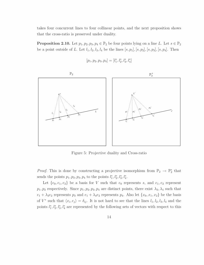
Proposition 2.10. Let p1, p2, p3, p4 ∈ P2 be four points lying on a line L. Let s ∈ P2

be a point outside of L. Let l1, l2, l3, l4 be the lines [s, p1], [s, p2], [s, p3], [s, p4]. Then

[p1, p2, p3, p4] = [l∗1, l∗2, l

∗3, l

∗4]

Figure 5: Projective duality and Cross-ratio

Proof. This is done by constructing a projective isomorphism from P2 → P∗2 that

sends the points p1, p2, p3, p4 to the points l∗1, l∗2, l

∗3, l

∗4.

Let {e0, e1, e2} be a basis for V such that e0 represents s, and e1, e2 represent

p1, p2 respectively. Since p1, p2, p3, p4 are distinct points, there exist λ3, λ4 such that

e1 + λ3e2 represents p3 and e1 + λ4e2 represents p4. Also let {x0, x1, x2} be the basis

of V ∗ such that 〈xi, ej〉 = δij . It is not hard to see that the lines l1, l2, l3, l4 and the

points l∗1, l∗2, l

∗3, l

∗4 are represented by the following sets of vectors with respect to this

14

basis.

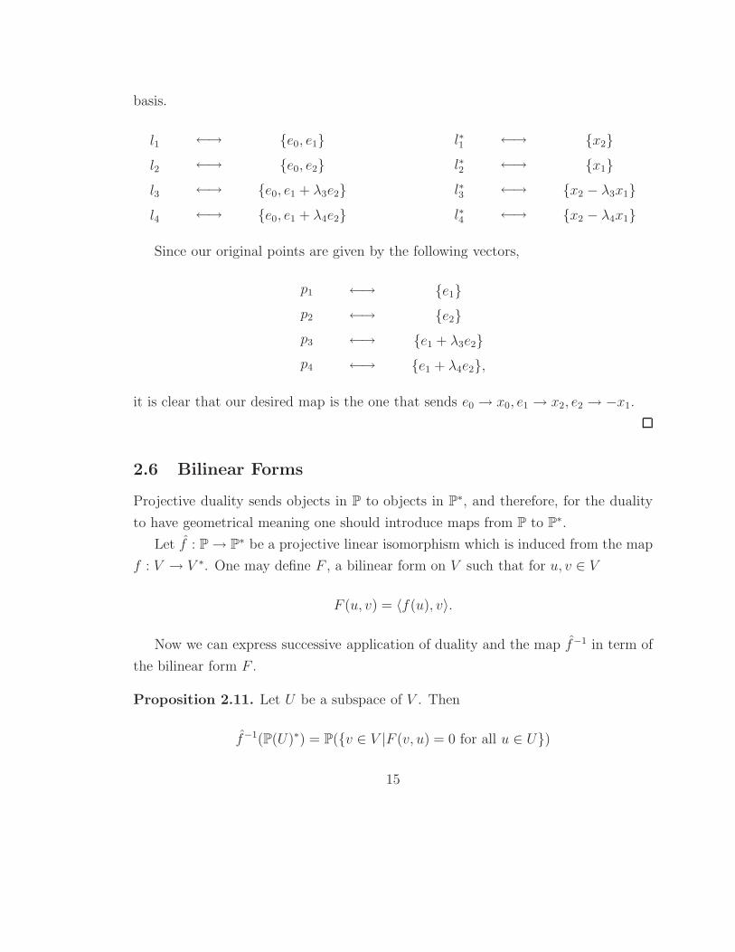
l1 ←→ {e0, e1} l∗1 ←→ {x2}

l2 ←→ {e0, e2} l∗2 ←→ {x1}

l3 ←→ {e0, e1 + λ3e2} l∗3 ←→ {x2 − λ3x1}

l4 ←→ {e0, e1 + λ4e2} l∗4 ←→ {x2 − λ4x1}

Since our original points are given by the following vectors,

p1 ←→ {e1}

p2 ←→ {e2}

p3 ←→ {e1 + λ3e2}

p4 ←→ {e1 + λ4e2},

it is clear that our desired map is the one that sends e0 → x0, e1 → x2, e2 → −x1.

2.6 Bilinear Forms

Projective duality sends objects in P to objects in P∗, and therefore, for the duality

to have geometrical meaning one should introduce maps from P to P∗.

Let f̂ : P→ P∗ be a projective linear isomorphism which is induced from the map

f : V → V ∗. One may define F , a bilinear form on V such that for u, v ∈ V

F (u, v) = 〈f(u), v〉.

Now we can express successive application of duality and the map f̂−1 in term of

the bilinear form F .

Proposition 2.11. Let U be a subspace of V . Then

f̂−1(P(U)∗) = P({v ∈ V |F (v, u) = 0 for all u ∈ U})

15

Proof. The claim follows after rewriting the right hand side of the equality in terms

of the map f .

{v ∈ V |F (v, u) = 0 for all u ∈ U} = {v ∈ V |〈f(v), u〉 = 0 for all u ∈ U} = f−1(U◦)

We can also work in the opposite direction. Given a bilinear form F on V , we can

define a map f : V → V ∗ as

f(v) = F (v, ∗) ∈ V ∗.

F is called non-degenerate if f is an isomorphism.

2.6.1 Symmetric Bilinear Forms

Now we consider a special case when the bilinear form F is symmetric.

Proposition 2.12. Given a non-degenerate symmetric bilinear form F on an

(n + 1)-dimensional vector space V over an algebraically closed field k, there exists a

basis {e0, e1, . . . , en} of V in which F is given by the identity matrix I, i.e.,

F (u, v) = utIv

Proof. The procedure of finding the desired basis is essentially the same as the Gram-

Schmidt method. Pick a vector v0 such that F (v0, v0) 6= 0. It is obvious that such

vector exists. Let e0 = v0/√

F (v0, v0). This is possible since k is algebraically closed.

Let

U0 = {e0}⊥ = {v ∈ V |F (v, u) = 0 for all u ∈ {e0} }.

Any vector v can be decomposed into

v = (v − F (v, e0)e0) + F (v, e0)e0,

16

where (v − F (v, e0)e0) is in {e0}⊥ and F (v, e0)e0 is in {e0}. Moreover this decompo-

sition is unique since

{e0} ∩ {e0}⊥ = {0}

and we can conclude that V = {e0}⊕U0. Also, F is non-degenerate on U0. Repeating

the same procedure on U0 we get e1 and U1. After finitely many steps, we end up

with a basis {e0, e1, . . . , en}.

Definition 5. Let F be a fixed symmetric bilinear form on V and P(U) ⊂ P(V ).

Then

P(U)⊥ = P({v ∈ V |F (v, u) = 0 for all u ∈ U})

and this duality is called polar duality.

The special name comes from the intimate connection between polar duality with

respect to the bilinear form F and the conic defined by the equation

F (v, v) = 0.

Lets investigate what polar duality looks like. Let a basis of V in which the

bilinear form F is given by the identity matrix I be fixed. Then for a given point

(v0 : v1 : . . . : vn) ∈ P(V ) we have

(v0 : v1 : . . . : vn)⊥ = {(x0 : x1 : . . . : xn) ∈ P(V )|n∑

i=0

xivi = 0}

The following remark tells us how much freedom we have while choosing the basis

in Proposition 2.12.

Definition 6. Let On(k) be the set of orthogonal n × n matrices A with entries ink, such that

AAt = I.

Remark. Let V be a vector space over a field k with a fixed basis and F be a bilinear

form given by the identity matrix I with respect to this basis. It is a well known

17

fact that the set of isomorphisms f of V which leave the bilinear form F invariant,

i.e., F (u, v) = F (f(u), f(v)), is given by the set On+1(k) if we associate linear maps

V → V with (n + 1)× (n + 1) matrices via the given basis.

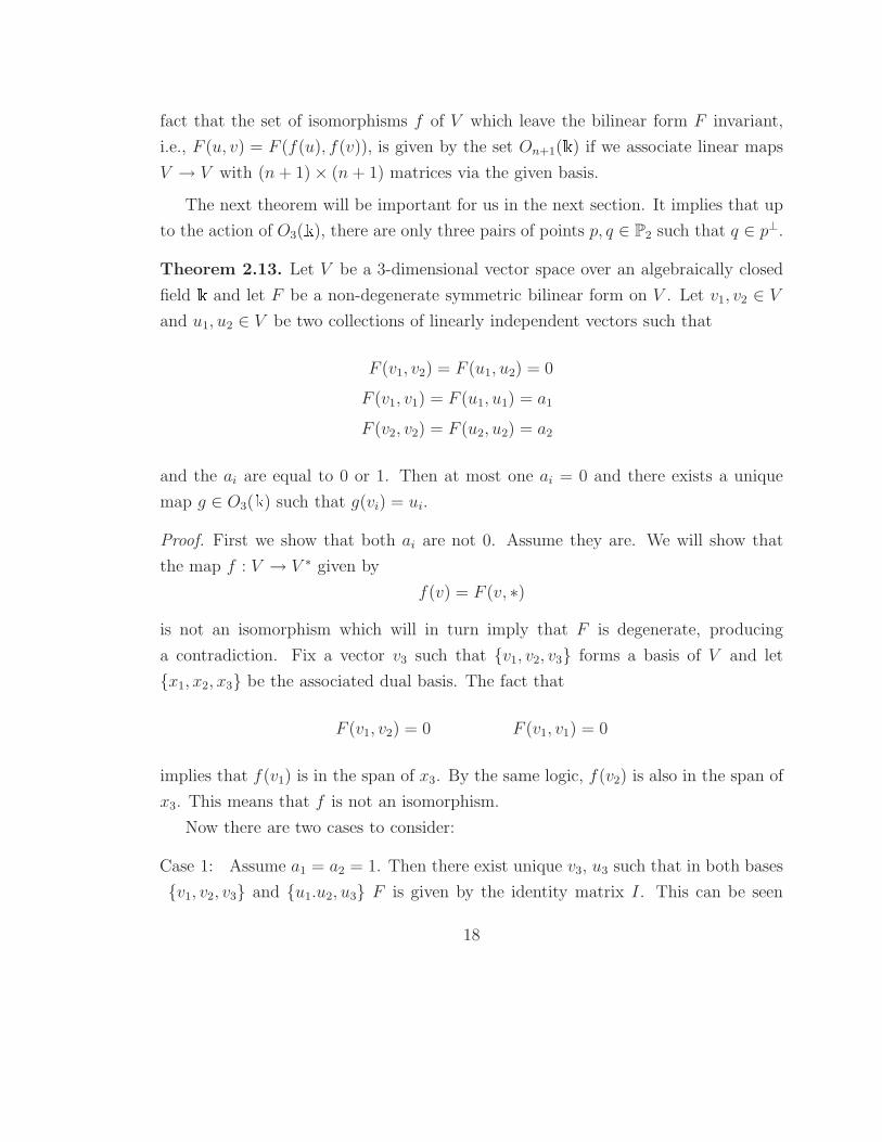
The next theorem will be important for us in the next section. It implies that up

to the action of O3(k), there are only three pairs of points p, q ∈ P2 such that q ∈ p⊥.

Theorem 2.13. Let V be a 3-dimensional vector space over an algebraically closed

field k and let F be a non-degenerate symmetric bilinear form on V . Let v1, v2 ∈ V

and u1, u2 ∈ V be two collections of linearly independent vectors such that

F (v1, v2) = F (u1, u2) = 0

F (v1, v1) = F (u1, u1) = a1

F (v2, v2) = F (u2, u2) = a2

and the ai are equal to 0 or 1. Then at most one ai = 0 and there exists a unique

map g ∈ O3(k) such that g(vi) = ui.

Proof. First we show that both ai are not 0. Assume they are. We will show that

the map f : V → V ∗ given by

f(v) = F (v, ∗)

is not an isomorphism which will in turn imply that F is degenerate, producing

a contradiction. Fix a vector v3 such that {v1, v2, v3} forms a basis of V and let

{x1, x2, x3} be the associated dual basis. The fact that

F (v1, v2) = 0 F (v1, v1) = 0

implies that f(v1) is in the span of x3. By the same logic, f(v2) is also in the span of

x3. This means that f is not an isomorphism.

Now there are two cases to consider:

Case 1: Assume a1 = a2 = 1. Then there exist unique v3, u3 such that in both bases

{v1, v2, v3} and {u1.u2, u3} F is given by the identity matrix I. This can be seen

18

from the proof of Proposition 2.12. In this case it is obvious that the only orthogonal

map with the desired conditions is the one that sends g(vi) = ui.

Case 2: Without loss of generality assume that a1 = 0 and a2 = 1. The outline of

the argument is the following. We will show that there are unique vectors v3 and u3

such that

F (v3, v1) = F (u3, u1) = 1

F (v3, v2) = F (u3, u2) = 0

F (v3, v3) = F (u3, u3) = 0

and that the sets {v1, v2, v3} and {u1, u2, u3} form bases for V . In this case the only

map satisfying the desired properties is again the one that sends g(vi) = ui. The

reason for that is that if g is orthogonal, then g(v3) must possess all the properties

that u3 has. Since we will show that u3 is the only vector with such properties, we

will have shown that g(v3) must be u3.

We will show the existence and uniqueness of v3. The argument for u3 is the same.

Since

F (v2, v1) = 0 F (v2, v2) = 1,

we know that v2 /∈ {v2}⊥.Therefore for {v1, v2, v3} to form a basis and for F (v3, v2) =

0, v3 must be of the following form

v3 = λ1v1 + λ2v′3

where λ2 6= 0 and v′3 is some vector such that v′

3 ∈ {v2}⊥. Since F (v3, v1) = 1 we

get that

F (v3, v1) = λ1F (v1, v1) + λ2F (v1, v′3) = λ2F (v1, v

′3) = 1

or equivalently

λ2 =1

F (v1, v′3)

19

which is defined and is unique since v′3 /∈ v⊥

1 = {v1, v2}. Also since F (v3, v3) = 0 we

get that

F (v3, v3) = λ21F (v1, v1) + 2λ1λ2F (v1, v

′3) + λ2

2F (v′3, v

′3)

= 2λ1 +F (v′

3, v′3)

F (v1, v′3)

2= 0

Which fixes λ1 uniquely.

2.6.2 Non-symmetric Bilinear Forms

In this section we investigate how many “distinct” non-symmetric forms there are.

We will focus on a three-dimensional vector space V over the field C since that is

what we need for the next section. The next lemma will be important for us in order

to analyze non-symmetric bilinear forms.

Definition 7. A bilinear form F on V is called skew-symmetric if F (u, v) = −F (v, u)

for all u, v ∈ V .

Lemma 2.1. Let F be a bilinear form on V . Then there exist a symmetric bilinear

form F+ and a skew-symmetric bilinear form F− such that

F = F− + F−.

Further, these bilinear forms are unique.

Proof. Fix a basis for V so that F can be associated with a matrix that we will again

call F . Then let

F− =F − F t

2F+ =

F + F t

2.

It is clear that F = F− + F+. The facts that F− is skew-symmetric and that F+ is

symmetric follow from the following relation

utFv = vtF tu.

20

Assume that there are distinct matrices F ′− and F ′

+ which have those properties. Then

F ′− + F ′

+ = F− + F+

F− − F ′− = F+ − F ′

+.

Since both sides of the last equality must be symmetric and skew-symmetric, we know

that they must be exactly 0. Therefore F ′− = F− and F ′

+ = F+.

The following is a classical lemma concerning skew-symmetric bilinear forms

Lemma 2.2. Let F be a skew-symmetric bilinear form on V . Let f : V → V ∗ be

defined as

f(v) = F (v, ∗).

Then rank of f is even.

Proof. Let U ⊂ V such that f |U : U → f(U) is an isomorphism. Our goal is to prove

that dim U = n is even. The first claim that we want to make is that we can consider

the map f |U as a map from U to U∗. The space V can be decomposed into

V = U ⊕ ker f,

and therefore V ∗ can be decomposed into

V ∗ = U∗ ⊕ (ker f)∗

where U∗ = (ker f)◦ and ker f ∗ = U◦. We need to show that f(U) ⊂ U∗. Assume it

is not. Then there exists u ∈ U such that f(u) /∈ (ker f)◦ or equivalently that there

exists v ∈ ker f such that 〈f(u), v〉 6= 0. But this is a contradiction since

〈f(u), v〉 = F (u, v) = −F (v, u) = −〈f(v), u〉 = 0.

By abuse of notation we write f for f |U . Pick any vector e1 in U . Consider the

21

following set,

e⊥1 = {v ∈ U |〈f(e1), v〉 = 0}

Since e⊥1 = f(e1)◦ we know that dim e⊥1 = n − 1. Also e1 ∈ e⊥1 since

F (e1, e1) = −F (e1, e1) = 0. This means that there exists a vector f1, not a mul-

tiple of e1 such that U = e⊥1 ⊕ {f1}. In particular 〈f(e1), f1〉 6= 0. By scaling f1, we

can assume that

〈f(e1), f1〉 = 1.

Let W1 = {e1, f1} and let

U1 = W⊥1 = {u ∈ U |〈v, u〉 = 0 for all v ∈ W1}

Since U1 = f(e1)◦ ∩ f(f1)

◦, we can conclude that dim U1 = n − 2 since it is an

intersection of two distinct (n− 1)-dimensional subspaces. Also U1 ∩W1 = {0} since

neither e1 or f1 are in U1 (since F (e1, f1) = 1). This means that

U = U1 ⊕W1.

Also, since F (u, v) = 0 for all u ∈ U1, v ∈ W1, we can consider the map

f |U1 : U1 → U∗1 .

Repeating the same procedure for U1 we get vectors {e2, f2}. After finitely many

steps we will have found basis for U which consists of {e1, e2, . . . , en2, f1, f2, . . . , fn

2}.

This basis is called symplectic basis of U . It is clear that dim U must be even.

Theorem 2.14. Let F be a non-degenerate non-symmetric bilinear form on a vector

space V = C3. Then there exists a basis in V with respect to which F has one of the

following forms:

22

Hφ =

cos φ sin φ 0

− sin φ cos φ 0

0 0 1

, J =

1 1 0

−1 0 0

0 0 1

, K =

1 1 0

−1 0 1

0 1 0

.

Also, for the case Hφ if 2φ is a multiple of π then the dimension of the group of

transformations preserving Hφ is 3, and otherwise it is 1.

Proof. The first thing that is important to see is that, given a basis {e1, e2, e3} of V ,

F is given by the matrix M = (aij), where aij = F (ei, ej).

Let F−, F+ be skew-symmetric and symmetric bilinear forms respectively such

that F = F− + F+. Let f−, f+ : V → V ∗ be the associated maps. We know that

F− 6= 0 since F is non-symmetric. Since by Lemma 2.2 the rank of f− is even, and

we know it is not 0, it must be 2. Let W = ker f−. Since rank of f− is 2, dim W = 1.

Case 1: F+|W 6= 0, rank f+ = 3.

Fix e3 ∈W such that F+(e3, e3) = 1. This is possible since F+|W 6= 0. Also since W

is one-dimensional, e3 is unique. Let Z = W⊥ with respect to F+, i.e.,

Z = {v ∈ V |F+(u, v) = 0 for all u ∈W}.

Fix e′1, e′2 ∈ Z such that F+(e′i, e

′j) = δij. This is possible by Proposition 2.12 since

F+ is a non-degenerate bilinear form on Z. There is one degree of freedom while

choosing e′1, e′2. This is the case since one only needs to fix the direction of e′1 (the

relation F+(e′1, e′1) = 1 defines the scaling). Therefore, e′1 could be thought of as

being chosen on P(Z) which is one dimensional. Also e′2 is fixed by the choice of e′1

and therefore does not add to the number of degrees of freedom.

Now let e1 = λe′1 and e2 = λe′2. We will find the value of λ such that F is given by

23

Hφ in the basis {e1, e2, e3}. In this basis F is given by

M =

λ2 λ2F−(e′1, e′2) 0

−λ2F−(e′1, e′2) λ2 0

0 0 1

There are four values of λ such that

det M = λ4 + λ4F−(e′1, e′2)

2 = 1,

since det M 6= 0 (F is non-degenerate). Picking any of those values of λ, we get

that M = Hφ where φ is given by cos φ = λ2. Also we know that λ 6= 0, therefore

φ 6= kπ/2. The choice of λ does not add to the number of degrees of freedom for the

choice of basis since there are finitely many choices for λ.

Case 2: F+|W 6= 0, rank f+ = 2.

Let e3 and Z be the same as in Case 1. Let f+ : V → V ∗ be the map associated

with F+. Since F+|W 6= 0, ker f+ ⊂ Z. Also, Z is two-dimensional and ker f+ is one

dimensional, therefore we can pick e1 ∈ Z − ker f+ such that F+(e1, e1) = 1. This

is possible since if v ∈ Z − ker f+, then F+(v, v) 6= 0, since otherwise v would be in

ker f+. Also fix some e′2 ∈ ker f+. Let e2 = λe′2. For an appropriate value of λ, in

the basis {e1, e2, e3}, F is given by the matrix J . In this basis F is given by

M =

1 λF−(e1, e′2) 0

−λF−(e1, e′2) 0 0

0 0 1

Therefore choosing

λ =1

F−(e1, e′2)

gives us the desired basis.

Case 3: F+|W 6= 0, rank f+ = 1.

24

In this case, fix e3 in the same way as in Case 1. Let f+ be the same as in Case 2.

Pick e1, e2 ∈ ker f+ such that F−(e1, e2) = 1. This is obviously possibly since F− is

non-degenerate on ker f+. In the basis {e1, e2, e3}, F is given by the matrix

Hπ2

=

0 1 0

−1 0 0

0 0 1

Now the question is how many degrees of freedom we have while choosing the sym-

plectic basis for the space ker f+. Clearly e1 can be chosen anywhere in ker f+ which

adds 2 degrees of freedom. Once e1 is chosen, to choose e2, we have to pick a point

on P(ker f+) (the scaling is fixed by the relation F−(e1, e2) = 1). Therefore, there

are 3 degrees of freedom while choosing the basis in this case.

Case:4 F+|W = 0, rank f+ = 3.

Let Z be the same as in the cases above. Fix some e′3 ∈ W . Consider the set

C = {v ∈ V |F+(v, v) = 0}. In a basis in which F+ is given by the matrix I, this set

is given by the equation

x21 + x2

2 + x23 = 0.

Therefore it does not belong to any two dimensional subspace. In particular C 6⊂ Z.

Let e′2 ∈ C − Z. Then F+(e′2, e′2) = 0 and F+(e′2, e

′3) 6= 0. By scaling e′2, we

may assume that F+(e′2, e′3) = 1. Take e1 ∈ {e

′3}

⊥ ∩ {e′2}⊥, where the orthogonal

compliment is taken with respect to F+.The set {e1, e′2, e

′3} forms a basis. This is

true because if e1 was a combination of e′2 and e′3, it could not be perpendicular to

both e2 and e3 since

F+(e′2, e′2) = 0 F+(e′3, e

′3) = 0 F+(e′2, e

′3) = 1

For this reason we have that F+(e1, e1) 6= 0, because otherwise e1 would be perpen-

dicular to all three basis vectors contradicting the non-degeneracy of f+. Therefore

we can scale e1 so that F+(e1, e1) = 1. Let e2 = λe′2 and e3 = λ−1e′3. For an appro-

25

priate value of λ, in the basis {e1, e2, e3}, F is given by the matrix K. In this basis

F is given by

M =

1 λF−(e1, e′2) 0

−λF−(e1, e′2) 0 1

0 1 0

Also F−(e1, e′2) 6= 0 because otherwise F− would be 0. Therefore setting

λ =1

F−(e1, e′2)

gives us the desired basis.

Case 5: F+|W = 0, rank f+ < 3.

Let f : V → V ∗ be the map associated with F . Let U be a one dimensional subspace

of V such that U ⊂ ker f+. If U = W , then F is degenerate since for any u ∈ U ,

f(u) = 0. Therefore assume that U 6= W . Let e1 ∈ U, e2 ∈ W, e3 ∈ V be such that

{e1, e2, e3} is a basis of V . Also let {x1, x2, x3} be the basis of V ∗ such that

〈xi, ej〉 = δij .

Then both f(e1) and f(e2) are in the span of {x3} since

F (e1, e1) = F (e1, e2) = F (e2, e2) = 0.

Also, F (e2, e2) = 0 since F+|W = 0. This contradicts the non-degeneracy of F .

The dimension of the group of transformations preserving the basis is equal to

number of degrees of freedom in the choice of the basis. Looking back at Case 1: and

Case 3:, we see that for the case Hφ, if 2φ is a multiple of π then the dimension of

the group of transformations preserving Hφ is 3, and otherwise it is 1.

26

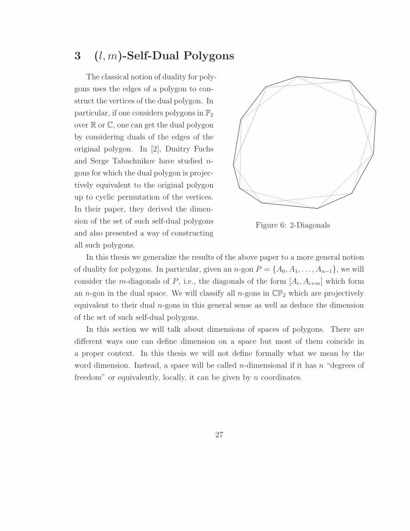
3 (l, m)-Self-Dual Polygons

The classical notion of duality for poly-

Figure 6: 2-Diagonals

gons uses the edges of a polygon to con-

struct the vertices of the dual polygon. In

particular, if one considers polygons in P2

over R or C, one can get the dual polygon

by considering duals of the edges of the

original polygon. In [2], Dmitry Fuchs

and Serge Tabachnikov have studied n-

gons for which the dual polygon is projec-

tively equivalent to the original polygon

up to cyclic permutation of the vertices.

In their paper, they derived the dimen-

sion of the set of such self-dual polygons

and also presented a way of constructing

all such polygons.

In this thesis we generalize the results of the above paper to a more general notion

of duality for polygons. In particular, given an n-gon P = {A0, A1, . . . , An−1}, we will

consider the m-diagonals of P , i.e., the diagonals of the form [Ai, Ai+m] which form

an n-gon in the dual space. We will classify all n-gons in CP2 which are projectively

equivalent to their dual n-gons in this general sense as well as deduce the dimension

of the set of such self-dual polygons.

In this section we will talk about dimensions of spaces of polygons. There are

different ways one can define dimension on a space but most of them coincide in

a proper context. In this thesis we will not define formally what we mean by the

word dimension. Instead, a space will be called n-dimensional if it has n “degrees of

freedom” or equivalently, locally, it can be given by n coordinates.

27

3.1 Notation

We are going to consider n-gons P = {A0, A1, . . . , An−1} where Ai ∈ P(C3) and indices

are considered modulo n, for which the vertices Ai, Ai+m, Ai+2m are not collinear for

all i for a fixed m. In particular this implies that 2m 6= n. Let Bmi = [AiAi+m] and

let Bmi

∗ ∈ P∗ be dual to Bmi .

Definition 8. Let P be an n-gon. We are going to say that P is an (l, m) self-dual

n-gon if there exists a projective isomorphism f̂ : P→ P∗ such that f̂(Ai) = Bmi+l

∗.

We will require that 0 ≤ l < n, 0 < m < n, l + m < n and 2l + m ≤ n. The

third inequality is not a restriction since if P is (l, m) self dual such that l + m ≥ n,

then P is also (l′, m′) self-dual where l′ = l + m mod n and m′ = n −m. The last

inequality is also not a restriction since if 2l + m > n, we can orient the polygon in

the other direction making it an (l′, m) self-dual polygon where l′ = n− (l + m) and

2l′ + m = 2n− (2l + m) < n.

Given an (l, m) self-dual n-gon with an associated projective isomorphism f̂ ,

we can fix an isomorphism f : C3 → C3∗ that induces f̂ , and a bilinear form

F : C3 × C3 → C such that F (v, u) = 〈f(v), u〉. While f̂ is unique, f and F

are unique up to multiplication by a non-zero constant. By abusing notation we are

going to let Ai mean both, a one dimensional subspace of C3 and a non-zero vector

in this subspace.

Definition 9. Let P be an n-gon P = {A0, A1, . . . , An−1}. Then kP ={A0, . . . , Akn−1}

is a (kn)−gon where Ai = Ai+rn for all 1 ≤ r < k. A polygon P will be called simple

if P 6= kP ′ for any k and any polygon P ′.

We will consider only simple polygons. This is justified by the fact that if P is

(l, m) self-dual, then so is kP .

3.2 The Case n = 2l + m

Theorem 3.1. Let P be an (l, m) self-dual n-gon. Then the bilinear form F is

symmetric if and only if n = 2l + m.

28

Proof. First notice that

F (Ai, Aj) = 0 ⇐⇒ 〈f(Ai), Aj〉 = 0⇐⇒ 〈Bmi+l

∗, Aj〉 = 0

⇐⇒ Aj ∈ Bmi+l = [Ai+lAi+l+m].

In particular, F (Ai, Ai+l) = F (Ai, Ai+l+m) = 0. Let F be symmetric. Then

F (Ai+l, Ai) = 0 ⇐⇒ Ai ∈ Bmi+2l (3.2.1)

F (Ai+l+m, Ai) = 0 ⇐⇒ Ai ∈ Bmi+2l+m

Figure 7: The case when F is symmetric.

Therefore, if F is symmetric, then Ai = Bmi+2l ∩ Bm

i+2l+m = Ai+2l+m. Since

2l+ m ≤ n, the polygon is simple and this is true for all i, it follows that n = 2l+m.

Now assume that n = 2l + m. From equation (3.2.1), we can conclude that

F (Ai+l, Ai) = F (Ai+l+m, Ai) = 0. Since the one-forms F (∗, Ai) and F (Ai, ∗) are

non-zero and have the same kernel, i.e., the linear span of {Ai+l, Ai+l+m}, they are

proportional. Let λi 6= 0 be such that F (Ai, ∗) = λiF (∗, Ai). In order to demonstrate

that F is symmetric, we need to show that λi = λj = 1 for some i 6= j. In the case

when such i, j exist, we can pick any vector e such that {Ai, Aj , e} forms a basis for

29

the vector space C3. Then for any x, y ∈ C3, if we expand F (x, y) in this basis, every

mixed term will contain either Ai or Aj and therefore can be reversed, proving that

F is symmetric.

Clearly if F (Ai, Ai) 6= 0 then λi = 1. We will show that there exist i, j such that

F (Ai, Ai) 6= 0 and F (Aj, Aj) 6= 0 which implies that λi = λj = 1 and consequently

that F is symmetric.

We will argue by contradiction. Assume that F (Ai, Ai) = 0 for at least (n− 1) val-

ues of i. Fix a value for i such that F (Ai, Ai) = 0. We will show that F (Ai+l, Ai+l) 6= 0

and F (Ai+l+m, Ai+l+m) 6= 0 which will contradict the assumption.

Figure 8: Assuming F (Ai, Ai) = F (Ai+l, Ai+l) = 0.

First notice that Ai ∈ Bmi+l = [Ai+lAi+l+m] since F (Ai, Ai) = 0. Assume that

F (Ai+l, Ai+l) = 0 then also F (Ai+l+m, Ai+l+m) = 0 since

F (Ai, Ai) = F (Ai+l, Ai+l) = F (Ai+l, Ai) = F (Ai, Ai+l) = 0

and Ai+l+m is in the span of {Ai, Ai+l} since these three points are collinear. Now

applying the same argument to points Ai+l and Ai+l+m we get

Ai+l ∈ Bmi+2l = [Ai+2l, Ai+2l+m] = [Ai+2l, Ai]

Ai+l+m ∈ Bmi+2l+m = [Ai+2l+m, Ai+2l+2m] = [Ai, Ai+m].

30

Thus, the points Ai+2l, Ai, Ai+m, Ai+l+m, Ai+l lie on a line. This is impossible

since Ai+2l, Ai, Ai+m cannot be collinear due to the non-degeneracy of the polygon P.

Therefore F (Ai+l, Ai+l) 6= 0.

The fact that F (Ai+l+m, Ai+l+m) 6= 0 then follows from the same line of reasoning:

if F (Ai+l+m, Ai+l+m) = 0, then F (Ai+l, Ai+l) = 0 since

F (Ai, Ai) = F (Ai+l+m, Ai+l+m) = F (Ai+l+m, Ai) = F (Ai, Ai+l+m) = 0,

and since Ai+l is in the span of {Ai, Ai+l+m}.

3.2.1 Explicit Construction

Here we are going to explicitly construct all (l, m) self-dual n-gons where n = 2l +m.

Since we know that the bilinear form F is symmetric, in appropriate coordinates the

duality becomes polar duality.

(a : b : c)→ (ax + by + cz = 0)

If we consider the chart Ux2 , then to get a polar line of a point one reflects the

point in the unit circle, then reflects it in the origin and then draws a line through

the given point perpendicular to its position vector. This can easily be seen from the

fact that in Ux2 , polar duality has the following form:

(a, b)→ (ax + by + 1 = 0).

Once we fix this polar duality, we consider polygons up to the action of O3(C), which

preserves polar duality.

Theorem 3.2. A polygon P = {A0, A1, ...An−1} is (l, m) self dual with respect to

polar duality where n = 2l + m if and only if Ai+l ∈ A⊥i for all i.

Proof. One direction is obvious. If P is an (l, m) self-dual n-gon, with respect to

polar duality, then Ai+l ∈ A⊥i = [Ai+l, Ai+l+m] by definition. For the other direction

31

assume that Ai+l ∈ A⊥i for all i. We need to show that Ai+l+m ∈ A⊥

i for all i. But

Ai = Ai+2l+m ∈ A⊥i+l+m =⇒ Ai+l+m ∈ A⊥

i .

The implication follows from the fact that the form F is symmetric.

Now we can construct all (l, m) self-dual n-gons where n = 2l + m. Pick A0 and

Al such that Al ∈ A⊥0 . By Theorem 2.13, there are three choices for A0, Al modulo

the action of O3(C). Then continue choosing Akl ∈ A⊥(k−1)l and Akl 6= A(k−2)l until

you get to A−l and choose A−l = A⊥−2l

⋂

A⊥0 . Also, when choosing A−2l, one should

ensure that A−2l 6= A0.

Figure 9: Construction of a (2, 2) self-dual 6-gon with respect to polar duality.

If you exhausted all vertices, then you are done. In this case the dimension of

the moduli space of all (l, m) self-dual n-gons is n− 3. All vertices except A0, Al, A−l

were chosen on a line with a finite number of points removed. If, on the other hand,

(l, n) 6= 1 where (l, n) denotes the greatest common divisor of l and n, then take A1

anywhere in the plane, and perform the same procedure starting from A1. Repeat

the same procedure starting from A2 and so on, until you generate all the points.

32

In this case the moduli space of (l, m) self-dual n-gons is again n− 3, since when

you perform this procedure starting from A1, you are picking A1 anywhere in the

plane, and the subsequent points on lines except for the last one which is fixed by

previous choices which gives you the dimensionn

(n, l). Therefore, the total dimension

isn

(l, n)− 3 + ((l, n)− 1)

n

(l, n)= n− 3.

3.3 The Case n 6= 2l + m

Let P = A0, A1, . . . , An−1 be an (l, m) self-dual n-gon where n 6= 2l + m. From

Theorem 3.1 we know that the bilinear form F is non-symmetric.

Definition 10. Let B be a line or a point in the space P. Define

B⊥ = {y ∈ P|F (x, y) = 0 for all x ∈ B},

and let G : P→ P be defined as G(B) = (B⊥)⊥.

In matrix form, G = F−1F t. This is the case since x⊥ = ker(xtF ) and

(x⊥)⊥ = {z|ytFz = ztF ty = 0 for all y ∈ x⊥ = ker(xtF )}.

Therefore, up to a constant, ztF t = xtF , or z = F−1F tx, since F is non-degenerate.

Lemma 3.1. If P is an (l, m) self-dual n-gon, then G(Ai) = Ai+2l+m.

Proof. We know that A⊥i = Bm

i+l, and therefore

(A⊥i )⊥ = (Bm

i+l)⊥ = Bm

i+2l ∩ Bmi+2l+m = Ai+2l+m.

It can also be seen that Gr = Id, where r =n

(n, 2l + m)since

Gr(Ai) = Ai+r(2l+m) = Ai

33

for all i, and a projective isomorphism that fixes four points in P2 is the identity.

Lemma 3.2. In appropriate coordinates, F = Hφ where φ =k

rπ and 1 ≤ k < 2r,

such that (k, r) = 1

Proof. Looking back at Theorem 2.14 we notice that

J−1J t =

−1 0 0

2 −1 0

0 0 1

, K−1Kt =

1 −2 0

0 1 0

2 −2 1

have infinite orders and therefore cannot equal G. Therefore, F = Hφ. Also,

G = F−1F t = H−2φ, and since Gr = Id, 2rφ is a multiple of 2π. The condition

(k, r) = 1 ensures that Gs 6= Id for all s < r which is necessary since the polygon is

simple.

This goes to say that an (l, m) self-dual n-gon, where 2l + m 6= n consists of

(n, 2l + m) regularn

(n, 2l + m)-gons.

3.3.1 Explicit Construction.

Given n, l, m with the necessary relations, we are going to construct all (l, m) self-dual

n-gons. Let r =n

(n, 2l + m), and fix k such that 1 ≤ k < 2r and (k, r) = 1. Let

φ =k

rπ. Fix a basis and let F = Hφ and consequently G = H−2φ. There are two

different cases to investigate based on the combinatorics of n, l and m.

Case 1: There exists a ∈ N such that a(2l + m) ∼= l mod n.

Proposition 3.3. Let P be an n-gon, and let l,m be fixed. Let a basis be fixed

and F = Hφ, where φ =k

rπ, 1 ≤ k < 2r and (k, r) = 1. Let G = F−2 and

suppose that Ai+2l+m = GAi for all i and that a(2l + m) ∼= l mod n. Then P

is (l, m) self-dual with respect to F if and only if AtiF

1−2aAi = 0 for all i.

34

Proof. We need to show that this condition is equivalent to

AtiFAi+l = At

iFAi+l+m = 0.

Since Ai+l = GaAi = F−2aAi,

AtiFAi+l = At

iF (F−2aAi) = AtiF

1−2aAi.

Also notice that (1− a)(2l + m) ∼= l + m mod n. Therefore

Ai+l+m = G1−aAi = F−2+2aAi

and

AtiFAi+l+m = At

iF (F−2+2aAi) = AtiF

−1+2aAi = AtiF

1−2aAi.

The last equality is obtained by taking the transpose of the entire expression

and noting that F t = F−1.

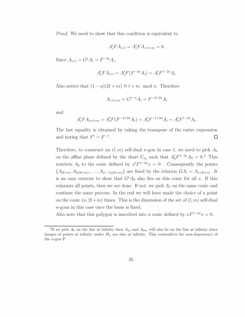
Therefore, to construct an (l, m) self-dual n-gon in case 1, we need to pick A0

on the affine plane defined by the chart Ux2 such that At0F

1−2aA0 = 0.3 This

restricts A0 to the conic defined by xtF 1−2ax = 0 . Consequently the points

{A2l+m, A2(2l+m), . . . , A(r−1)(2l+m)} are fixed by the relation GAi = Ai+2l+m. It

is an easy exercise to show that GsA0 also lies on this conic for all s. If this

exhausts all points, then we are done. If not, we pick A1 on the same conic and

continue the same process. In the end we will have made the choice of a point

on the conic (n, 2l+m) times. This is the dimension of the set of (l, m) self-dual

n-gons in this case once the basis is fixed.

Also note that this polygon is inscribed into a conic defined by xF 1−2ax = 0.

3If we pick A0 on the line at infinity then Am and A2m will also lie on the line at infinity sinceimages of points at infinity under Hφ are also at infinity. This contradicts the non-degeneracy ofthe n-gon P.

35

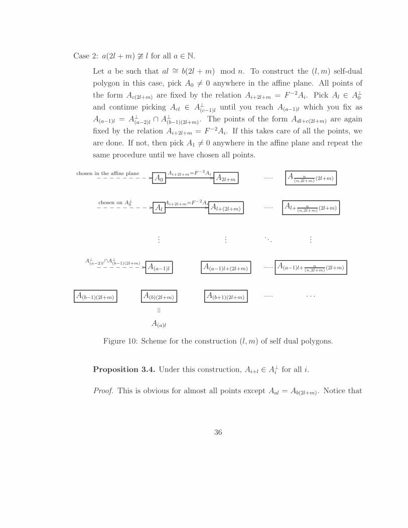
Case 2: a(2l + m) � l for all a ∈ N.

Let a be such that al ∼= b(2l + m) mod n. To construct the (l, m) self-dual

polygon in this case, pick A0 6= 0 anywhere in the affine plane. All points of

the form Ac(2l+m) are fixed by the relation Ai+2l+m = F−2Ai. Pick Al ∈ A⊥0

and continue picking Acl ∈ A⊥(c−1)l until you reach A(a−1)l which you fix as

A(a−1)l = A⊥(a−2)l ∩ A⊥

(b−1)(2l+m). The points of the form Adl+c(2l+m) are again

fixed by the relation Ai+2l+m = F−2Ai. If this takes care of all the points, we

are done. If not, then pick A1 6= 0 anywhere in the affine plane and repeat the

same procedure until we have chosen all points.

chosen in the affine plane//_________ A0

Ai+2l+m=F−2Ai// A2l+m

...... A n(n,2l+m)

(2l+m)

chosen on A⊥

0//_________ Al

Ai+2l+m=F−2Ai// Al+(2l+m) ...... Al+ n

(n,2l+m)(2l+m)

......

......

A⊥

(a−2)l∩A⊥

(b−1)(2l+m)//________ A(a−1)l A(a−1)l+(2l+m) ...... A(a−1)l+ n

(n,2l+m)(2l+m)

A(b−1)(2l+m) A(b)(2l+m)

||

A(b+1)(2l+m) ...... . . .

A(a)l

Figure 10: Scheme for the construction (l, m) of self dual polygons.

Proposition 3.4. Under this construction, Ai+l ∈ A⊥i for all i.

Proof. This is obvious for almost all points except Aal = Ab(2l+m). Notice that

36

Ab(2l+m) = F−2A(b−1)(2l+m) and since A(a−1)l ∈ A⊥(b−1)(2l+m)

0 = At(b−1)(2l+m)FA(a−1)l = (F 2Ab(2l+m))

tFA(a−1)l

= At(a−1)lFAb(2l+m)

Which exactly implies that Aal ∈ A⊥(1−a)l.

Proposition 3.5. Under this construction, Ai+l+m ∈ A⊥i for all i.

Proof. Since Ai ∈ A⊥i−l and Ai−l = F 2Ai+l+m,

0 = Ati−lFAi = (F 2Ai+l+m)tFAi

= AtiFAi+l+m.

This shows that our polygon is (l, m) self-dual, and it is clear why this

construction takes care of all (l, m) self-dual polygons since every

restriction was a necessity for the polygon to be (l, m) self-dual. Notice also

that if 2l ∼= b(2l + m) mod n, then we do not choose Al on A⊥0 but fix it as

Al = A⊥0 ∩A⊥

−m.

We can now deduce that the dimension of the set of (l, m) self-dual polygons

is again (n, 2l + m) once the basis is fixed. In Diagram 10, each row represents

an equivalence class of points with indices differing by a multiple of (2l + m).

During the algorithm, we encounter the same number of degrees of freedom as

the number of equivalence classes that we define. For the first equivalence class

we choose A0 anywhere on the plane, for all other equivalence classes we pick a

point on a line except for the last equivalence class which is fixed by previous

choices. The total number of these equivalence classes is (n, 2l + m).

Proposition 3.6. The dimension of the moduli space of all (l, m) self-dual polygons

where 2l + m 6= n is (n, 2l + m) − 3 for n = 2(2l + m), and (n, 2l + m) − 1 for

n 6= 2(2l + m).

37

Proof. We have shown that if the basis is fixed then the dimension of the set of (l, m)

self-dual polygons is (n, 2l + m). From this we have to subtract the dimension of

the group of transformations that preserve F . From the proof of Theorem 2.14, this

dimension is 1 if 2φ is not a multiple of π and 3 if 2φ is a multiple of π. Since

φ =k

rπ where (k, r) = 1, 2φ is a multiple of π if and only if r =

n

(n, 2l + m)= 2, or

equivalently 2(2l + m) = n since 2l + m < n.

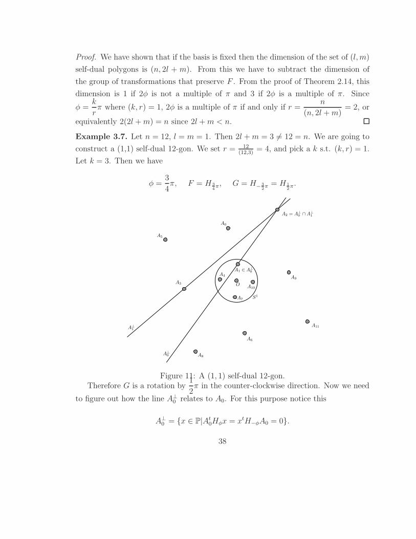
Example 3.7. Let n = 12, l = m = 1. Then 2l + m = 3 6= 12 = n. We are going to

construct a (1,1) self-dual 12-gon. We set r = 12(12,3)

= 4, and pick a k s.t. (k, r) = 1.

Let k = 3. Then we have

φ =3

4π, F = H 3

4π, G = H− 3

2π = H 1

2π.

Figure 11: A (1, 1) self-dual 12-gon.Therefore G is a rotation by

1

2π in the counter-clockwise direction. Now we need

to figure out how the line A⊥0 relates to A0. For this purpose notice this

A⊥0 = {x ∈ P|At

0Hφx = xtH−φA0 = 0}.

38

Therefore A⊥0 is the polar dual of H−φA0. Since in our case φ = 3

4π, in order to get

A⊥0 we need to rotate A0 by 3

4π in the clockwise direction, then reflect the point in

the unit circle, then reflect it in the origin and then draw a line through the resulting

point perpendicular to its position vector.

Fix the point A0 in the plane. Pick a point A1 on A⊥0 and fix A2 = A⊥

0 ∩A⊥1 . The

rest of the points are fixed by the relation

Ai+2l+m = Ai+3 = H 12πA0.

This gives us an (1, 1) self-dual 12-gon as in the Figure 11.

39

4 Geometric Surprises

This thesis was partially motivated by recently discovered relations between n-gons

which are inscribed into a projective conic and those having the self-duality property

discussed in Section 3. These relations have originally been discovered via computer

experimentation. One can read more about these relations in [9].

Let χn and χ∗n be the sets of n-gons in P2 and P∗

2 respectively. We define a map

Tk : χn → χ∗n in the following way. Let P = {A0, A1, . . . , An−1} be a polygon and let

Bmi

∗ = [AiAi+m]∗ be the duals of the m-diagonals of P . Then

Tm(P ) = {Bm0

∗, Bm1

∗, . . . , Bmn−1

∗}.

We will also use an abbreviation, Tab = Ta ◦ Tb. This makes sense, since the map Tm

is also well defined on χ∗n.

Given two n-gons P ∈ P(V ) and Q ∈ P(U), we will say that P and Q are

equivalent, or P ∼ Q, if there exists a projective isomorphism f : P(V ) → P(U)

which sends P to Q preserving the order of vertices, but perhaps rotating them.

Proposition 4.1. The map Tm is an involution up to rotation of vertices and pro-

jective isomorphisms. In other words

Tmm(P ) ∼ P

for all n-gons P .

Proof. Let P = {A0, A1, . . . , An−1}. Then Tm(P ) = {Bm0

∗, Bm1

∗, . . . , Bmn−1

∗} and

Tmm(P ) = {[Bm0

∗, Bmm

∗], [Bm1

∗, Bm1+m

∗], . . . , [Bmn−1

∗, Bmm−1

∗]}

= {Am, Am+1, . . . , Am−1}

40

Definition 11. A non-singular projective conic C in P(V ) is given by the equation

F (v, v) = 0

for some non-degenerate symmetric bilinear form F on V .

By Proposition 2.12, we know that any two non-singular conics are projectively

equivalent. A polygon P = {A0, A1, . . . , An−1} will be called inscribed if there exists

a projective conic C such that Ai ∈ C for all i. We will also call a polygon P ,

m-self-dual, if it is (l, m) self-dual for some l.

We are now able to state the theorem which should astound the reader.

Theorem 4.2. Let P ⊂ CP2 be an inscribed n-gon. Then the following statements

hold

If P is a 6-gon then P ∼ T2(P )

If P is a 7-gon then P ∼ T212(P )

If P is an 8-gon then P ∼ T21212(P )

If P is a 9-gon then P ∼ T13131(P )

If P is a 12-gon then P ∼ T3434343(P )

An equivalent formulation of Theorem 4.2 is that if P is an inscribed n-gon then

the following statements hold

If P is a 6-gon then P is 2-self-dual

If P is a 7-gon then T2(P ) is 1-self-dual

If P is an 8-gon then T12(P ) is 2-self-dual

If P is a 9-gon then T31(P ) is 1-self-dual

If P is a 12-gon then T343(P ) is 4-self-dual

The reason why the two collections of statements are equivalent is that Tm is an

involution. One might notice some patterns in the theorem and wonder if they are

41

beginnings of some infinite patterns. As far as computer simulations go, no similar

patterns were noticed for n-gons where n is greater than 12.

Although Theorem 4.2 has a purely geometrical flavor, only the first two state-

ments gave in to geometrical arguments. The rest of the theorems had to be proved

computationally. These proofs are not very insightful, and one should still ask oneself

whether there is some underlying reasons why this theorem holds and why there are

no similar statements for n-gons where n is greater than 12. In this thesis we will

present the geometrical proofs.

4.1 Corner Invariants

In order to analyze polygons up to projective isomorphisms, we shall introduce coordi-

nates on the space of polygons which are preserved under projective transformations.

Definition 12. Let P = {A0, A1, . . . , An−1} be an n-gon. Consider the

following construction at a point Ai. Let P = [Ai−2, Ai−1] ∩ [Ai, Ai+1],

R = [Ai−1, Ai−2] ∩ [Ai+1, Ai+2], and Q = [Ai−1, Ai] ∩ [Ai+1, Ai+2] as in Figure 12.

Then the corner invariants at the point Ai are defined as

pi = [Ai−2, Ai−2, P, R] qi = [R, Q, Ai+1, Ai+2]

where [∗, ∗, ∗, ∗] stands for cross-ratio.

It is clear that corner invariants stay invariant under projective transformations

since cross-ratio is invariant under projective transformations. Also, corner invariants

define the n-gon uniquely. By Proposition 2.4, the first four points can be fixed

anywhere in the plane. All the following points can be constructed afterward using

corner invariants. The corner invariants are not independent. They have to satisfy

certain relations in order for the polygon to be closed.

It turns out that the map T1 behaves nicely with respect to corner invariants.

This will be important for us in one of the geometric proofs.

42

Figure 12: Corner invariants at a point Ai.

Proposition 4.3. Let P = {A0, A1, . . . , An−1} be an n-gon. Let pi, qi be the corner

invariants of P and let p∗i , q∗i be the corner invariants of T1(P ). Then

p∗i = qi q∗i = pi+1

Proof. We will only show the first relation. The second relation is obtained by ap-

plying the first relation to the polygon T1(P ) and realizing that the polygon T11(P )

is the rotation of P by one vertex.

To calculate p∗i we need to construct P ∗ = [B1i−2

∗, B1

i−1∗] ∩ [B1

i

∗, B1

i+1∗] and

R∗ = [B1i−1

∗, B1

i−2∗] ∩ [B1

i+1∗, B1

i+2∗] as in Figure 13. In the dual space, [B1

i−2∗, B1

i−1∗]

is the line passing through points B1i−2

∗and B1

i−1∗

which in the original space takes

the form of a point of intersection of B1i−2 and B1

i−1. Also the intersection of two

lines l1, l2 in the dual space takes the form of a line passing through l∗1 and l∗2 in the

original space.

By Proposition 2.10, the cross-ratio of the four lines equals the cross ratio of four

points which are intersections of those four lines with some fixed line. Therefore

43

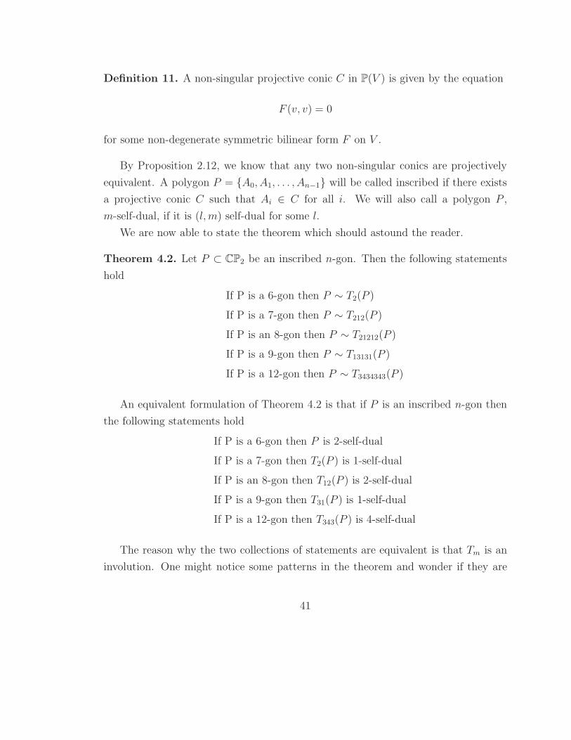
Figure 13: Corner invariants of the dual polygon.

projecting lines B1i−2, B

1i−1, P

∗, Q∗ onto the line [Ai+1, Ai+2] gives us

p∗i = [B1i−2

∗, B1

i−1∗, P ∗, Q∗] = [R, Q, Ai+1, Ai+2] = qi.

4.2 Geometrical Proofs

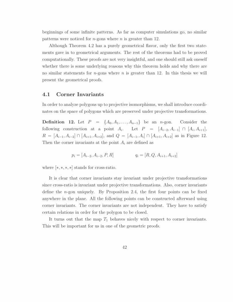
At the heart of the geometrical proofs that will be presented in this section, lies a

classical theorem that we will state without a proof.

Theorem 4.4 (Pascal’s Theorem). Let C be a conic. Let A1, A2, A3, B1, B2, B3 ∈ C

44

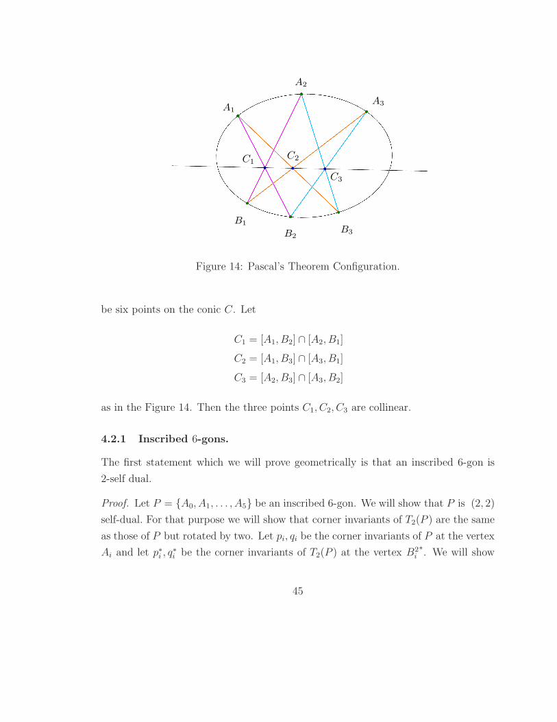
Figure 14: Pascal’s Theorem Configuration.

be six points on the conic C. Let

C1 = [A1, B2] ∩ [A2, B1]

C2 = [A1, B3] ∩ [A3, B1]

C3 = [A2, B3] ∩ [A3, B2]

as in the Figure 14. Then the three points C1, C2, C3 are collinear.

4.2.1 Inscribed 6-gons.

The first statement which we will prove geometrically is that an inscribed 6-gon is

2-self dual.

Proof. Let P = {A0, A1, . . . , A5} be an inscribed 6-gon. We will show that P is (2, 2)

self-dual. For that purpose we will show that corner invariants of T2(P ) are the same

as those of P but rotated by two. Let pi, qi be the corner invariants of P at the vertex

Ai and let p∗i , q∗i be the corner invariants of T2(P ) at the vertex B2

i

∗. We will show

45

that

p0 = p∗2.

The equality of the rest of the corner invariants follows from analogous reasonings.

The first thing that we need to do is find the eight points, whose cross-ratios

determine p0 and p∗2. Let P ∗ = [B10∗, B1

1∗] ∩ [B1

2∗, B1

3∗], R∗ = [B1

0∗, B1

1∗] ∩ [B1

3∗, B1

4∗]

as in Figure 15. Then from the definition of corner invariants,

p∗2 = [B20∗, B2

1∗, P ∗, R∗].

Figure 15: Calculation of p∗2

If we let Z = [A3, A5]∩[A0, A2], X = [A4, A2]∩[A3, A5] and Y = [A0, A4]∩[A3, A5],

and then project the four lines B20 , B

21 , P

∗, R∗ onto the line [A3, A5], we get that

p∗2 = [Z, A3, X, Y ].

Now we need to find p0. If we let P = [A4, A5] ∩ [A0, A1], R = [A4, A5] ∩ [A1, A2],

then by definition

p0 = [A4, A5, P, R].

We need to show that p0 = p∗2 or equivalently

[A4, A5, P, R] = [Z, A3, X, Y ].

46

Figure 16: Calculation of p0

The cross-ratio is preserved under projections. In order to show that the two cross-

ratios are the same, we are going to construct a map ξ from the line [A3, A5] to the

line [A4, A5] such that ξ is a composition of two projections and

ξ(Z) = R ξ(A3) = P ξ(X) = A5 ξ(Y ) = A4.

This will complete the proof since ξ leaves the cross-ratio invariant and also

[X,Y,Z,W] = [W,Z,Y,X] for any quadruple of points {X, Y, Z, W}. (This can be

directly verified from the definition of cross-ratio.)

Let S = [A3, A5] ∩ [A1, A2], and let ξ = πS ◦ πA0 , where πA0 is the projection

from the line [A3, A5] onto the line [A4, A2] through the point A0, and where πS is

the projection of the line [A4, A2] onto the line [A4, A5] through the point S.

We need to verify four images of the map ξ. Three of those images are obvious.

ξ(Z) = πS ◦ πA0(Z) = πS(A2) = R

ξ(X) = πS ◦ πA0(X) = πS(X) = A5

ξ(Y ) = πS ◦ πA0(Y ) = πS(A4) = A4

47

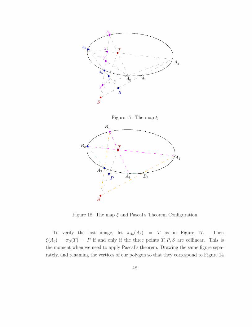
Figure 17: The map ξ

Figure 18: The map ξ and Pascal’s Theorem Configuration

To verify the last image, let πA0(A3) = T as in Figure 17. Then

ξ(A3) = πS(T ) = P if and only if the three points T, P, S are collinear. This is

the moment when we need to apply Pascal’s theorem. Drawing the same figure sepa-

rately, and renaming the vertices of our polygon so that they correspond to Figure 14

48

of Pascals theorem, we get precisely the statement that we need, namely that T, P, S

are collinear.

4.2.2 Inscribed 7-gons.

Now we will show that if P is an inscribed 7-gon, then T2(P ) is 1-self-dual. This

proof is due to Richard Schwartz.

Figure 19: P and T12(P ).

Proof. Let P = {A0, A1, . . . , A6} be an inscribed 7-gon. We will show that T12(P ) is

(3, 1) self-dual. Clearly if T12 is (3, 1) self-dual, then T2(P ) ∼ T12(P ) and therefore

T2 is also (3, 1) self-dual. Let T12(P ) = {C0, C1, . . . , C6}. It is easy to verify that

Ci = [Ai, Ai+2] ∩ [Ai+1, Ai+3]. Let pi, qi be the corner invariants of T12(P ) at the

vertex Ci.

From Proposition 4.3, it follows that T12(P ) is (3, 1) self-dual if and only if pi = qi+3

and qi = pi+4 for all i. We will show that p0 = q3. The other relations follow from

the same logic.

49

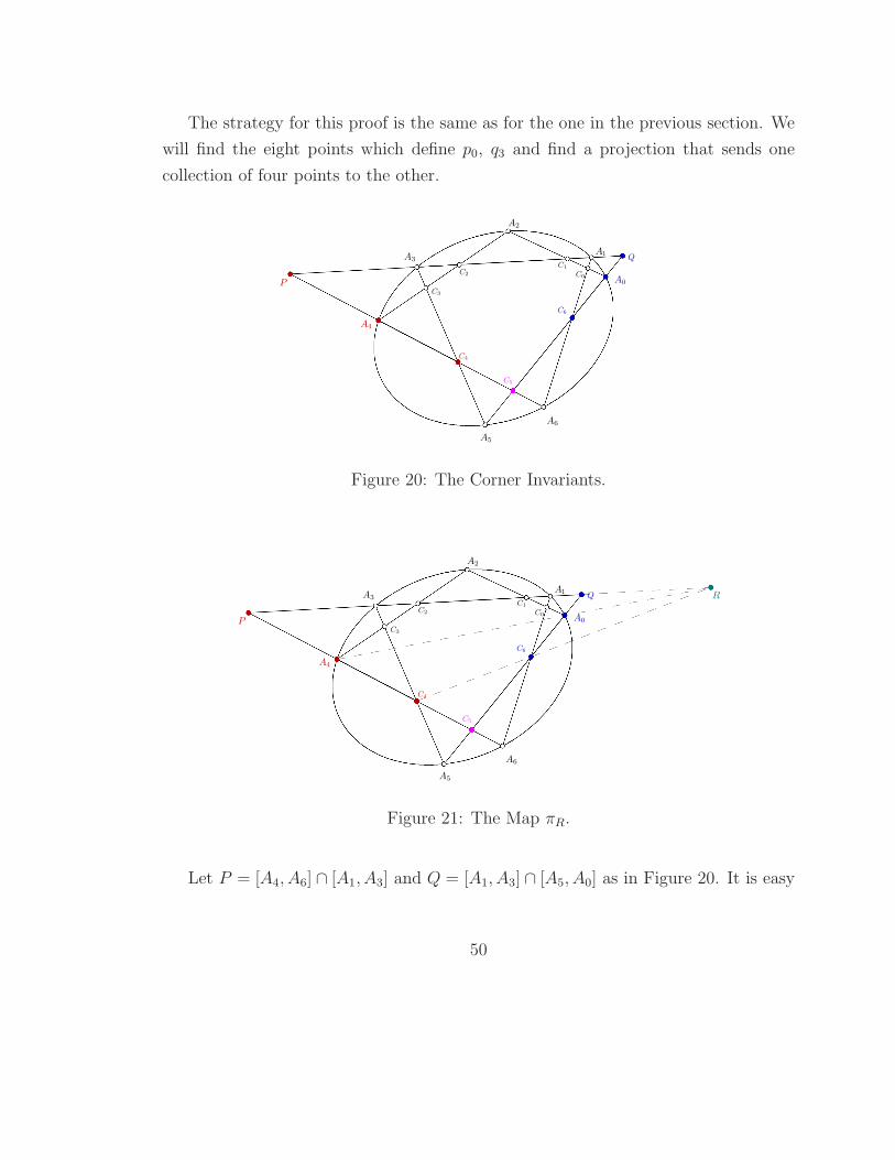
The strategy for this proof is the same as for the one in the previous section. We

will find the eight points which define p0, q3 and find a projection that sends one

collection of four points to the other.

Figure 20: The Corner Invariants.

Figure 21: The Map πR.

Let P = [A4, A6] ∩ [A1, A3] and Q = [A1, A3] ∩ [A5, A0] as in Figure 20. It is easy

50

to check that

p0 = [C5, C6, A0, Q] q3 = [C5, C4, A4, P ].

We need to find a point R such that πR is a projection from the line [A0, A5] onto

the line [A4, A6] such that

πR(C5) = C5 πR(C6) = C4 πR(A0) = A4 πR(Q) = P.

Let R = [A4, A0]∩ [A3, A1]. By Pascals theorem, R, C6, C4 are collinear. Taking a

close look at Figure 21 one can easily see that πR is the desired map and p0 = q3.

51

5 Conclusion

There is a computational proof for the statements of theorem 4.2 involving hexagons,

heptagons and octagons due to Sergei Tabachnikov that requires one to calculate the

action of the map T2 in terms of corner invariants. The rest of the cases were proved

by brute force computation using Mathematica and are due to Richard Schwartz and

Sergei Tabachnikov. The paper with the details of these proofs should appear in the

near future.

In this thesis we considered fixed points of the map Tm. A natural generalization

of this analysis would be to consider the fixed points of the map Tab for some natural

numbers a, b. It turns out that the dynamics of the map Tab are very rich. The

following papers deal solely with the dynamics of the map T12 : [3–8]. Further, one

can consider dynamics of the map Ta1,a2,...,amfor some fixed sequence a1, a2, . . . , am.

Another direction where one might take this research is to analyze the “geometric

surprises”. One might try to find a joint proof for all statements of Theorem 4.2 and

find out why the pattern stops at 12-gons.

52

List of Figures

1 An affine chart . . . . . . . . . . . . . . . . . . . . . . . . . . . . . . 3

2 A cone in R3 . . . . . . . . . . . . . . . . . . . . . . . . . . . . . . . 6

3 Projection in P2 . . . . . . . . . . . . . . . . . . . . . . . . . . . . . . 7

4 Cross-Ratio under projections . . . . . . . . . . . . . . . . . . . . . . 11

5 Projective duality and Cross-ratio . . . . . . . . . . . . . . . . . . . . 14

6 2-Diagonals . . . . . . . . . . . . . . . . . . . . . . . . . . . . . . . . 27

7 The case when F is symmetric. . . . . . . . . . . . . . . . . . . . . . 29

8 Assuming F (Ai, Ai) = F (Ai+l, Ai+l) = 0. . . . . . . . . . . . . . . . . 30

9 Construction of a (2, 2) self-dual 6-gon with respect to polar duality. . 32

10 Scheme for the construction (l, m) of self dual polygons. . . . . . . . . 36

11 A (1, 1) self-dual 12-gon. . . . . . . . . . . . . . . . . . . . . . . . . . 38

12 Corner invariants at a point Ai. . . . . . . . . . . . . . . . . . . . . . 43

13 Corner invariants of the dual polygon. . . . . . . . . . . . . . . . . . 44

14 Pascal’s Theorem Configuration. . . . . . . . . . . . . . . . . . . . . . 45

15 Calculation of p∗2 . . . . . . . . . . . . . . . . . . . . . . . . . . . . . 46

16 Calculation of p0 . . . . . . . . . . . . . . . . . . . . . . . . . . . . . 47

17 The map ξ . . . . . . . . . . . . . . . . . . . . . . . . . . . . . . . . . 48

18 The map ξ and Pascal’s Theorem Configuration . . . . . . . . . . . . 48

19 P and T12(P ). . . . . . . . . . . . . . . . . . . . . . . . . . . . . . . . 49

20 The Corner Invariants. . . . . . . . . . . . . . . . . . . . . . . . . . . 50

21 The Map πR. . . . . . . . . . . . . . . . . . . . . . . . . . . . . . . . 50

53

References

[1] M. Berger, Geometry 1, Springer, 1987.

[2] D. Fuchs and S. Tabachnikov, Self-dual polygons and self-dual curves, Funct. Anal. and Other

Math. 2 (2009), 203–220.

[3] M. Glick, The pentagram map and Y-patterns, ArXiv e-prints (May 2010), available at 1005.

0598.

[4] V. Ovsienko, R. Schwartz, and S. Tabachnikov, The Pentagram map: a discrete integrable system,

Comm. Math. Phys., in print.

[5] V. Ovsienko, R. Schwartz, and S. Tabachnikov, Quasiperiodic motion for the pentagram map,

Electron. Res. Announc. Math. Sci. 16 (2009), 1–8.

[6] R. Schwartz, The pentagram map, Experiment. Math. 1 (1992), no. 1, 71–81.

[7] R. Schwartz, The pentagram map is recurrent, Experiment. Math. 10 (2001), no. 4, 519–528.

[8] R. Schwartz, Discrete monodromy, pentagrams, and the method of condensation, Journal of Fixed

Point Theory and Applications 3 (2008), no. 2, 379–409.

[9] R. Schwartz and S. Tabachnikov, Elementary surprises in projective geometry, The Mathematical

Intelligencer (2009).

54