M. Belloli, A. Collina, M. Belloli, A. Collina, F.F. RestaRestaPolitecnico di Milano Politecnico di Milano

O.I.T.A.F.O.I.T.A.F. SEMINARSEMINAR

Grenoble 27 Grenoble 27 AprilApril 20062006

CablesCables vibrationsvibrations due due toto windwind actionaction

Presentation• Main topic of the presentation is the vibrations of cables

due to wind action.

• The research group of Politecnico di Milano, leaded by Prof. Giorgio Diana (CIGRE member) deals with these topics since several years. This short presentation illustrates some of the most important concepts in this field and take advantage also from the experiences/tests/development of simulation tools gained from the whole group.

• Main of the phenomena herein presented concern vibrations of cables in electrical power transmission lines, but the general concepts can be applied to any general problem of cables/ropes exposed to wind action.

Main phenomena related to wind effects on cables/ropes vibration

• Aeolian vibration (vortex shedding): alternate formation of vortices in the downstream wake of the cable.

• Vibration due to turbulent wind (buffeting): mainly related to forcing effects due to variation of wind speed both in module and direction.

• Aeroelastic instability (galloping): irregular shape, due f.i. to ice deposit (ice galloping), can lead to modification of cable profile, and unstable oscillations can occur.

• Wake induced vibrations (bundle galloping): typical for cables fitted in bundles (grouped in 2, 3, 4, or more formation), as occurs in electrical power transmission lines.

Aeolian vibrations: phenomenology

• Aeolian vibrations occur both on single and bundled conductors and are due to the vortex shedding excitation.

• Two symmetric wakes are normally created behind the section of the body, but at higher speed they are replaced by a formation of cyclic alternating vortices.

Aeolian vibrations on cable/circular cylinders

svf Sd

=

ffss== vortexvortex sheddingshedding frequencyfrequency (Hz)(Hz)

S= S= StrouhalStrouhal numbernumber 0.1850.185÷÷0.20.2

v= v= windwind speedspeed (m/s)(m/s)

d= d= cablecable diameterdiameter (m)(m)

• Vortex shedding phenomenon is characterised by a frequency fs, depending on dimension, wind speed and a constant (S) depending on the shape.

Aeolian vibrations on elastically suspendedcircular cylinders

• The alternate shed of vortex is equivalent to a sinusoidal forceacting on the cylinder, originating oscillations in a direction normal to the wind direction.

• When the vortex shedding frequency (Strouhal frequency fs=0.2v/d) equals the natural frequency fc of the cylinder, a resonance condition occurs.

f/fCIL

Aeolian vibration: lock in phenomenon

• Vibrating cylinder: outside the lock-in conditions the vortices shed according to the Strouhal relation, inside the lock-in range the frequency of vortex shedding is driven by the motion of the cylinder itself.

• The cause is the vibration of the cylinder that in a close interval to fc=fs, is able to organizes the shed of the vortices, that is sincronised on the natural frequency of the cylinder.

Lock-in region

1s

c c

f vSf d f=

Lock-in range, vibration amplitude limited to the diameter and hysteretic phenomena are the main characteristics of vortex induced vibration.

0.0

0.1

0.2

0.3

0.4

0.5

0.6

0.7

0.8

0.7 0.8 0.9 1.0 1.1 1.2 1.3 1.4 1.5 1.6 1.7 1.8 V/Vs

u/D

DownUp

Aeolian vibration: lock in phenomenon

Aeolian vibration: general aspects• Aeolian vibrations occur almost on any transmission line, for

low to moderate winds.• They are characterised by small amplitudes of vibration (one

conductor diameter) with frequency between 5 and 100 Hz, depending on the conductor size and tensile load.

• Aeolian vibrations cause an alternate bending strain of the conductor at the suspension clamp (where bending stiffness is no more negligible) and, depending on the strain level, may cause fatigue failures of the cable strands.

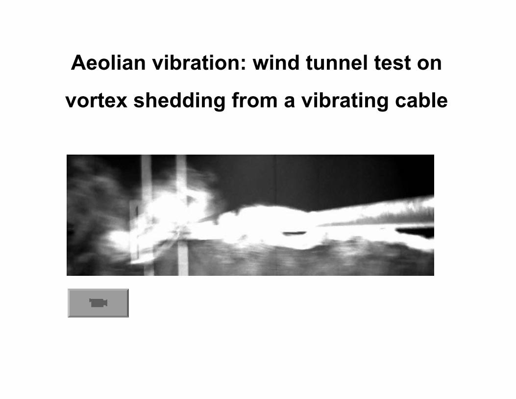
Aeolian vibration: wind tunnel test on

vortex shedding from a vibrating cable

• Considering a cable or a rope, different natural frequencies exist. In the case of sag much less than the span length, are according to the formula:

Natural frequency of a taut cable

nn Tf

2L m=

ffnn = = frequencyfrequency of the of the nn--thth mode (Hz)mode (Hz)

n = n = orderorder of the of the vibrationvibration modemode

L = L = spanspan lengthlength (m)(m)

T = T = cablecable tensiletensile loadload ( N)( N)

m = m = cablecable//roperope mass per mass per unitunit lengthlength (Kg/m)(Kg/m)

Vibration modes of a taut cable

Vibration modes of a taut cable

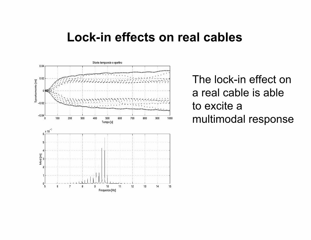
Lock-in effects on real cables

The lock-in effect on a real cable is able to excite a multimodal response

Aeolian vibrations appearance

• Considering a cable or a rope under aeolian vibration, different natural frequencies are excited. As a consequence, the appearance of the recorded vibration is characterised by beating phenomena.

Max Max amplitudeamplitude = a= a11+a+a2 2

MinMin amplitudeamplitude = a= a11--aa2 2

frequencyfrequency = (f= (f11+f+f22)/2)/2

frequencyfrequency of the of the beatingbeating = (f= (f11--ff22)/2)/2

Aeolian vibrations appearance: beatingAeolian vibrations appearance: beating

BeatingBeatingexamplesexamples

Aeolian vibrations appearance: beatingAeolian vibrations appearance: beating

Evaluation of amplitudes of vibration• Vibration amplitude due to aeolian vibration can be evaluated

by means of several approach.• Simplified approaches applicable outside lock-in region.• Power balance approach, applicable to multimodal analysis. It

makes a balance between the power introduced by the wind (P), and the power dissipated by the structural damping. This method relies upon experimental data that can be obtained from wind tunnel tests.

• Equivalent oscillator model, which simulates the interaction between the rope and the fluid, by means of an auxiliary oscillator with non linear damping.

Power input from wind

Power dissipated bystructural damping

Amplitude of vibrationfor each mode

Build-up analysis to evaluate power input

The power imparted by the blowing wind tothe cylinder can be evaluated withbuild-up tests

22

3 4 22P m uPf D L D D

π δ = =

%

Use of power input from wind to evaluatevibration amplitude

22

3 4 22P m uPf D L D D

π δ = =

%

f = f = frequencyfrequency ((HzHz);); u = u = amplitudeamplitude of of vibrationvibration

D = D = roperope diameterdiameter;; δδ = = logarithmiclogarithmic decrementdecrement

m = m = roperope mass per mass per unitunit lengthlength (Kg/m)(Kg/m)

P = power inputP = power input = = specificspecific power input power input P%

Sectional models

Flexible models

Flexible cable in single mode of vibration

Power input measured in wind tunnel

Aeolian vibrationsAeolian vibrations can be easily controlled by can be easily controlled by adding damping to the cable, in the form of adding damping to the cable, in the form of dampers and spacerdampers and spacer--dampers. This is feasible for dampers. This is feasible for electric power transmission lineselectric power transmission lines

Space turbulence

Time turbulence

Windspeed

time

Cable dynamic response to turbulent wind

Characteristics of turbulent wind• Wind turbulence depends on:• Mean wind speed: it decreases with increasing speed• Type of surrounding: open terrain, flat surfaces, suburban

area, forest, etc.• Turbulence index is the ration between speed variation and

mean wind speed.

VVmedmed

VVRMSRMSTurbulence index

I = VRMS/VMED

I(mean)= 0.164

Km/h

WIND SPEED

I(mean)= 0.1

(m/s)WIND SPEED

VRMS

VRMS

San NicolasSan Nicolas

ArgentinaArgentina

Porto Porto TolleTolle

ItaliaItalia

Characteristics of turbulent wind: index of turbulence dependence on wind speed

Table I – Influence of surface roughness on parameters relating to

wind structure near the ground

TYPE OF SURFACE Power law

exponent

Gradient

height

Drag

coefficient

Open terrain with very few obstacles: e.g. open grass or farmland

with few trees, hedgerows and other barriers etc.; prairie; tundra;

shores and low island of inland lakes; desert.

0.16 274 0.005

Terrain uniformly covered with obstacles 30-50 ft in height: e.g.

residential suburbs; small towns; woodland and scrub. Small field

with bushes, trees and hedges.

0.28 395 0.015

Terrain with large and irregular objects: e.g. centers of large cities;

very broken country with many windbreaks of tall trees, etc.

0.40 520 0.050

Characteristics of turbulent wind: surrounding features

Flat terrain, no obstacles to the wind-> Minimum turbulence

Characteristics of turbulent wind: surrounding features

CultivatedCultivated country, country, flatflat terrainterrain withwith few, few, smallsmallobstaclesobstacles toto the the windwind -> LowLow turbulenceturbulence

Characteristics of turbulent wind: surrounding features

Ondulated terrain, forest -> High turbulence

Characteristics of turbulent wind: surrounding features

• Wind mean speed and direction vary with the region and with the period of the year:

• It is important to know the mean wind speed and direction distribution typical of the region were the structure will be placed in order to evaluate the risk for the different types of wind excited vibrations and take the suitable countermeasures.

• Wind can be treated as an ergodic and stationary quantity, and the related statistics (mean value, rmsvalue, frequency distribution, etc.) can be defined on a specific site.

Characteristics of turbulent wind: statistics

It is analytically represented by Weibull and Rayleigh probability density functions with parameters estimated on the base of the experimental data

Aeolian vibrations

Subspan oscillations

galloping

Characteristics of turbulent wind: statistics

Simulation of turbulent wind space-time field• Power Spectral Density (PSD) function define the distribution

of power along the frequencies as, for instance, Von Karmanformulation.

• A single time history of wind is generated, according to the amplitudes obtained from the PSD, using the wave superposition method. The phase of each harmonic component is random in the interval 0-2π.

• The generation of the wind field transversally to wind directioncan be carried out according to the spatial correlation function, or using numerical filters, like ARMA models.

• The final results is the distribution in space and time of the wind incident the structure.

• The wind forces can be then calculated according to the quasi steady theory and applied to the structure.

2,

5 62

4

1 70.8

U W

ux

fLf UPSD

fLU

σ =

+

( ), ,1,

( , ) cos 2i i n o i nj N

U x t u n f tπ ϕ=

= +∑

i nC x fi eη − ∆=

ϕ1,n ϕi-1,n

ui-1,n

ui,n

Coherent part

Not coherentpart

Im

Re

Simulation of turbulent wind space-time fieldPSD definition Generation of time history

Spatial correlation to generate the subsequent section

Complete space-time wind field

Simulation of response to turbulent wind• Several approaches can be followed, all can be divided into

two main categories: time domain methods and frequency domain methods.

• Time domain methods can consider non linearity of aerodynamic actions and eventually of the structure, but are more time consuming. They can not easily account for the dependence of the aeroelastic coefficients on the reduced wind speed.

• Frequency domain methods can easily account for dependence on reduced wind speed but relies on the superposition principle: non linearities (from aeroelastic terms formulation and from structure behaviour) can not be accounted for. Less time consuming.

• Both can use modal representation of the structure, when applicable according to the kind of structure.

Simulation of response to turbulent wind

U

w

y& z&

U

wz&

y&

Vrel

FL FD

Vrel

2

2

1212

D D rel

L L rel

F C V

F C V

ρ

ρ

=

=

Lagrangian components in the FE model or in the modal approach

Time domain integration of the equations of motion

Quasi static correctedtheory (q.s.c.t.)

Simulation of response to turbulent wind• Q.s.c.t. accounts for the forcing effects due to turbulence and

for the aeroelastic behaviour of the cable, i.e. the mutual interaction that exist between the aerodynamic forces and the motion of the cable (or the structure in general) itself.

• Time domain methods can consider the full formulation of the q.s.c.t.

• Frequency domain methods require the linearisation of the formulation (f.i. as in Scanlan formulation), separating the pure buffeting terms, from the aeroelastic ones. They are the most used in engineering practice.

• Due to the interaction between cable (structure) and wind, static instability (divergence) and dynamic instability conditions can occur.

• A linear analysis, based on the q.s.c.t. can account for these phenomena, that is typical of bluff-bodies, characterised by non aerodynamic shapes.

• In the case of cables/ropes, this condition may occur when ice deposit on the surface modifies the regular circular shape.

• In this case ice-galloping can occur for high wind speeds for high wind speeds (V>15 (V>15 m/sm/s) and is characterised by high amplitudes of ) and is characterised by high amplitudes of vibration (up to the conductor sag) with low frequency.vibration (up to the conductor sag) with low frequency.

Aeroelastic instability

Aeroelastic instability: ice galloping

[ ]2 21 1cos sin2 2y L D LO LO DO

yF F F C DV DV K CV

α α ρ ρ= − ≅ + −&

• To investigate instability condition, first the aerodynamic term are linearised, separating a constant contribution, and a linear contribution:

• having considered that the non linear term can be linearisedin the following way, with respect to the angle of attack αand then to the vertical motion y of the cylinder:

2 2 2 2 cos 1 sin tanrel

LD DO L LO LO LO

yV V y VV

CC C C C K K

α α α α α

αα

= + ≅ ≅ ≅ = ≅

∂= + = + =

∂

&&

K

Aeroelastic instability: ice galloping

• Lift coefficient CLchange dramatically its trend according to the type of profile. In particular the sign of the derivative with respect to the angle of attack a changes its sign.

• Aerodynamic profile (like a wing section) and a bluff body (like a rope covered by ice deposit) have opposite behaviour.

CL

α

Aeroelastic instability: ice galloping• The following linear equation is obtained:

• in which the sign of the damping term gives the indication of the possibility of existence of a dynamic instability:

• In the case of KLO>CDO, a instability wind speed will always exist. Its value depends upon the value of the structural damping too.

( ) 20

12 0n DO LOm y h C K y ym

ω ω + + − + = && &

( )2 2

1 12 2

n nLO DO INST

LO DO

mh mhK C or VDV D K Cω ω

ρ ρ− > >

−

Aeroelastic instability: ice galloping

• Wake induced vibrations (subspan oscillations) occur only on bundles with at least one couple of sub-conductors with one in the wake of the other.

• The phenomenon occurs for medium to high wind speeds (V > 10m/s) and then is not so common as aeolian vibrations.

•• Amplitudes of vibration (up to the bundle Amplitudes of vibration (up to the bundle separation) with low frequency (0.7separation) with low frequency (0.7÷÷2 Hz).2 Hz).

Wake induce vibrations

Concluding remarks• Several kinds of phenomena are related to wind

action on cables and ropes.• Aeolian vibration (vortex shedding) are the most

common, and cover a wide range of frequencies and usually occur for low range of wind speed (v<10m/s). Low amplitude of vibration are generally induced.

• Vibration due to turbulent wind (buffeting) depend mainly on the surrounding characteristics, which determines the statistical characteristics of the wind. The whole speed range is interested, and the first frequencies of the rope are involved.

• Aeroelastic instability on cable can occur only in the case of ice deposit (ice galloping) and relatively high speed (V>15m/s). High amplitude at low frequency are induced.