Lynbrook Robotics Team, FIRST 846 Control System Miniseries - Lecture 4 06/11/2012.

Lynbrook Robotics Team, FIRST 846

Control System Miniseries- Lecture 4

06/11/2012


Math Difference, Difference Quotient & Derivative Summation & Integration

Physics Force analysis – free body diagram Newton’s Laws Acceleration, velocity and displacement

Block Diagram Operation Transfer function

Note: In this lecture, we bring advance concepts to in a simple and understandable way. As long as you read the material carefully, for most contents, you have no problem to understand them.

Lecture 4 Basic Math/Physics Concepts Used in System Modeling


Linear Motion of a Point Position and Displacement of a Point Velocity of a Point Acceleration of a Point

Angular Motion of a Point Angular Position and Displacement of a Point Angular Velocity of a Point Angular Acceleration of a Point

Outline – A Point Motion


Position Position is coordinates of a point in a

coordinate system (1D, 2D, or 3D) Displacement

Displacement is position difference between a point and another point.

ΔXBA = XB – XA

Different from distance, displacement has direction.

Unit: m (or mm, inch, feet, etc.)

Position and Displacement of a Point

X (m)

XA XB

-1 0 1 2-2 3

A BC

XC

Example: • An object moves to B position

from A position• Then, move to C from B.

Point Position Motion Displacement

A XA = 1 m

B XB = 3 m A -> B ΔXBA = XB – XA = 3 m – 1 m= 2 m

C XC = -2 B -> C ΔXCB = XC – XB = -2 m – 3 m = -5 m


Angular Position Angular position is angular

coordinates of a point in a coordinate system (2D, or 3D)

Angular Displacement Angular displacement is angular

position difference between a point and another point.

ΔθBA = θB – θA

Angular displacement has direction. Unit: Radian (or degree)

Angular Position and Displacement of a Point

Example: • An object rotates to B position

from A position• Then, rotates to C from B.

A (θA = π/3 Rad)

B (θB = 2π/3 Rad)

C (θC = -π/4 Rad)

Point Position Motion Displacement

A θA = π/3 Rad

B θB = 2π/3 Rad A -> B ΔθBA = θB – θA = 2π/3 Rad – π/3 Rad

= π/3 Rad

C θC = -π/4 Rad B -> C ΔθCB = θC – θB = -π/4 Rad– 2π/3 Rad

= -11π/2 Rad


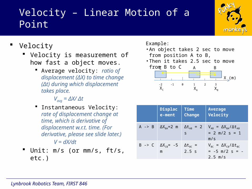
Velocity Velocity is measurement of how fast

a object moves. Average velocity: ratio of

displacement (ΔX) to time change (Δt) during which displacement takes place.

Vavg = ΔX/ Δt

Instantaneous Velocity: rate of displacement change at time, which is derivative of displacement w.r.t. time. (For derivative, please see slide later.)

V = dX/dt Unit: m/s (or mm/s, ft/s, etc.)

Velocity – Linear Motion of a Point

Example: • An object takes 2 sec to move from

position A to B, • Then it takes 2.5 sec to move from B to C

Displace-ment

Time Change

Average Velocity

A -> B ΔXBA=2 m ΔtAB = 2 s VAB = ΔXBA/ΔtAB = 2 m/2 s = 1 m/s

B -> C ΔXCB= -5 m ΔtBC = 2.5 s VBC = ΔXCB/ΔtBC = -5 m/2 s = -2.5 m/s

X (m)

XA XB

-1 0 1 2-2 3

A BC

XC


Angular velocity Angular velocity is measurement of

how fast a point rotates about a fixed point.

Average angular velocity: ratio of angular displacement (Δθ) to time change (Δt) during which angular displacement takes place.

ωavg = Δθ/ Δt

Instantaneous angular velocity: rate of angular displacement change at time, which is derivative of displacement w.r.t. time. (For derivative, please see slide later.)

ω = dθ/dt Velocity has direction. Unit: rad/s (or deg/s, rpm, etc)

Angular Velocity – Rotation Motion of a Point



Motion Angular Displacement

Time Change

Angular Velocity

A -> B ΔθBA = π/3 Rad

ΔtAB = 2 s ωAB = ΔθBA/ΔtAB = 2 Rad/2 s = 1 rad/s

B -> C ΔθCB = -11π/2 Rad

ΔtBC = 2 s ωBC = ΔθCB/ΔtBC = -5 Rad/2 s = -2.5 Rad/s

A (θA = π/3 Rad)

B (θB = 2π/3 Rad)

C (θC = -π/4 Rad)


Acceleration Acceleration is measurement of how

fast velocity changes. Average acceleration: ratio of velocity

changes (ΔV) to time change (Δt) which velocity change takes place

aavg= ΔV/ Δt

Instantaneous Acceleration: Rate of velocity change at time, which is derivative of velocity w.r.t. time. For derivative, please see slide later.

Acceleration has direction Unit: m/s2 (or ft/s2, g, etc.)

Acceleration – Linear Motion of a Point



Velocity Change

Time Change

Average Acceleration

A -> B

ΔVBA=VB-VA

=2 m/s – 0 =2 m/s

ΔtAB = 2 s aAB = ΔVBA/ΔtAB = 2 m/s/2 s = 1 m/s2

B -> C ΔVCB=VC-VB

=-2 m/s –2 m/s = -4 m/s

ΔtBC = 2 s aBC = ΔVCB/ΔtBC = -4 m/s/2 s = -2 m/s2

X (m)

XA XB

-1 0 1 2-2 3

A BC

XC

VA= 0 VB = 2 m/sVC = - 2 m/s


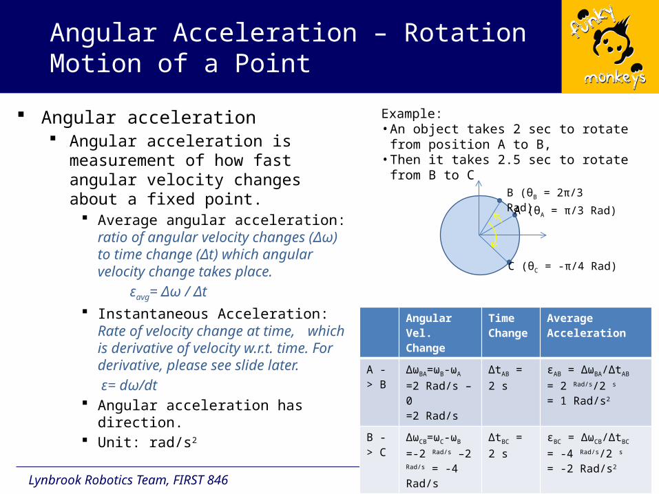
Angular acceleration Angular acceleration is measurement

of how fast angular velocity changes about a fixed point.

Average angular acceleration: ratio of angular velocity changes (Δω) to time change (Δt) which angular velocity change takes place.

εavg= Δω / Δt

Instantaneous Acceleration: Rate of velocity change at time, which is derivative of velocity w.r.t. time. For derivative, please see slide later.

ε= dω/dt Angular acceleration has direction. Unit: rad/s2

Angular Acceleration – Rotation Motion of a Point

Angular Vel. Change

Time Change


A -> B

ΔωBA=ωB-ωA

=2 Rad/s – 0 =2 Rad/s

ΔtAB = 2 s εAB = ΔωBA/ΔtAB = 2 Rad/s/2 s = 1 Rad/s2

B -> C ΔωCB=ωC-ωB

=-2 Rad/s –2 Rad/s = -4 Rad/s

ΔtBC = 2 s εBC = ΔωCB/ΔtBC = -4 Rad/s/2 s = -2 Rad/s2

Example: • An object takes 2 sec to rotate from

position A to B, • Then it takes 2.5 sec to rotate from B to C

A (θA = π/3 Rad)

B (θB = 2π/3 Rad)

C (θC = -π/4 Rad)


Point Position Instantaneous Velocity

Time Motion Time Change

Displacement Velocity Change

Average Velocity


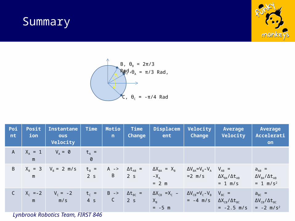
A XA = 1 m VA = 0 tA = 0

B XB = 3 m VB = 2 m/s tB = 2 s A -> B ΔtAB = 2 s ΔXBA = XB –XA

= 2 mΔVBA=VB-VA

=2 m/sVAB = ΔXBA/ΔtAB = 1 m/s

aAB = ΔVBA/ΔtAB = 1 m/s2

C XC =-2 m VC = -2 m/s tC = 4 s B -> C ΔtBC = 2 s ΔXCB =XC – XB = -5 m

ΔVCB=VC-VB

= -4 m/sVBC = ΔXCB/ΔtBC = -2.5 m/s

aBC = ΔVCB/ΔtBC = -2 m/s2

Summary

X (m)

XA XB

-1 0 1 2-2 3

A BC

XC

VA= 0 VB = 2 m/sVC = - 2 m/s

tC = 4 s tA = 0 s tB = 2 s


Point Position Instantaneous Velocity

Time Motion Time Change

Displacement Velocity Change

Average Velocity


A XA = 1 m VA = 0 tA = 0

B XB = 3 m VB = 2 m/s tB = 2 s A -> B ΔtAB = 2 s ΔXBA = XB –XA

= 2 mΔVBA=VB-VA

=2 m/sVAB = ΔXBA/ΔtAB = 1 m/s

aAB = ΔVBA/ΔtAB = 1 m/s2

C XC =-2 m VC = -2 m/s tC = 4 s B -> C ΔtBC = 2 s ΔXCB =XC – XB = -5 m

ΔVCB=VC-VB

= -4 m/sVBC = ΔXCB/ΔtBC = -2.5 m/s

aBC = ΔVCB/ΔtBC = -2 m/s2

Summary

A, θA = π/3 Rad,

B, θB = 2π/3 Rad,

C, θC = -π/4 Rad


Derivative is the rate of changes of one variable with respect to another. Rate is ratio when the changes of relevant variables are infinitesimal. For a number of frequently used functions, derivative can be calculated by

following simple three steps Difference Difference Quotient Derivative

Simply speaking, integration is summation. However, its exact definition can not be simply described because there

are two types of integration Definitive integration In-definitive integration

Integration of a couple of function can be demonstrated with approximation of summation. Integration of other functions needs more math preparation.

However, in-definitive integration is reverse calculation of derivative. So, we take short cut to calculate integration by knowing original function of a derivative.

Appendix: Derivative and Integration


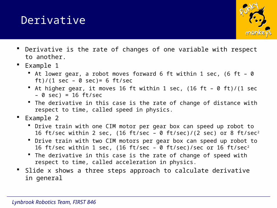
Derivative is the rate of changes of one variable with respect to another.

Example 1 At lower gear, a robot moves forward 6 ft within 1 sec, (6 ft – 0 ft)/(1 sec –

0 sec)= 6 ft/sec At higher gear, it moves 16 ft within 1 sec, (16 ft – 0 ft)/(1 sec – 0 sec) = 16

ft/sec The derivative in this case is the rate of change of distance with respect to

time, called speed in physics. Example 2

Drive train with one CIM motor per gear box can speed up robot to 16 ft/sec within 2 sec, (16 ft/sec – 0 ft/sec)/(2 sec) or 8 ft/sec2

Drive train with two CIM motors per gear box can speed up robot to 16 ft/sec within 1 sec, (16 ft/sec – 0 ft/sec)/sec or 16 ft/sec2

The derivative in this case is the rate of change of speed with respect to time, called acceleration in physics.

Slide x shows a three steps approach to calculate derivative in general

Derivative


Simply speaking, integration is summation. Example 1

A robot moves at 1 ft/sec speed. Over 10 sec, this robot will move 10 ft, (1 ft + 1 ft + … + 1 ft) =10 ft.

Example 2 A robot average speed is 1 ft/sec at 1st sec, 2 ft/sec at 2nd sec, 3 ft/sec at

3rd sec,…, etc. Basically, it is speeding up (accelerates). 5 sec later, this robot speed will reach

Integration


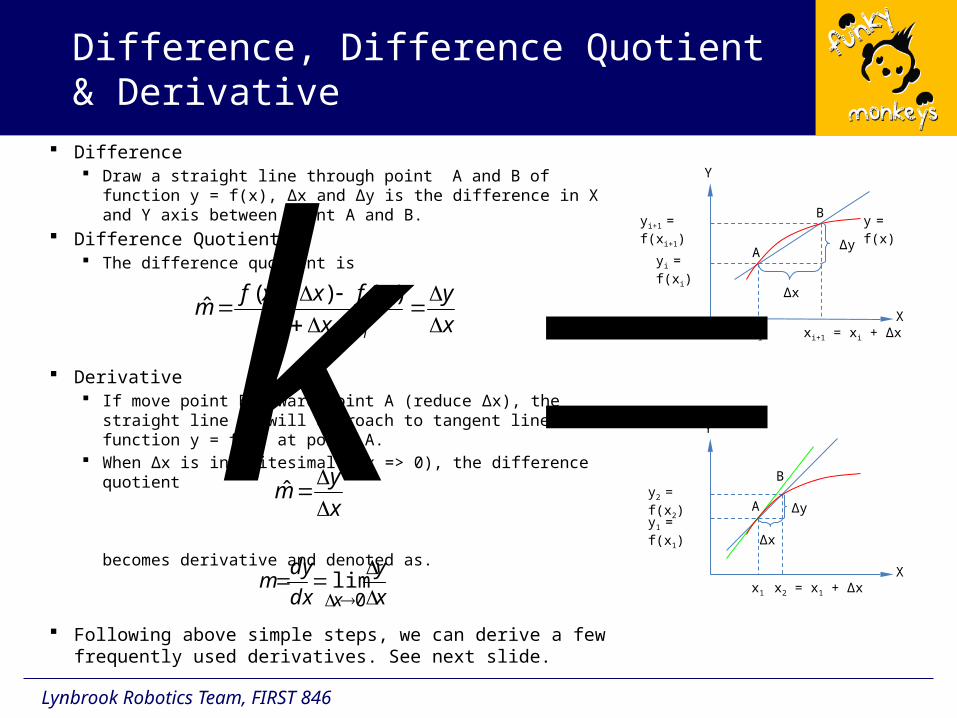
Difference Draw a straight line through point A and B of function y =

f(x), Δx and Δy is the difference in X and Y axis between point A and B.

Difference Quotient The difference quotient is

Derivative If move point B toward point A (reduce Δx), the straight line

AB will approach to tangent line of function y = f(x) at point A.

When Δx is infinitesimal (Δx => 0), the difference quotient

becomes derivative and denoted as.

Following above simple steps, we can derive a few frequently used derivatives. See next slide.

Difference, Difference Quotient & Derivative

x1 x2 = x1 + Δx

y1 = f(x1)

y2 = f(x2)

Δx

Δy

X

Y

A

B

xi xi+1 = xi + Δx

yi = f(xi)

yi+1 = f(xi+1)

Δx

Δy

X

Y

A

By = f(x)

k x

y

xxx

xfxxfm

ii

ii

)()(

ˆ

x

y

dx

dym

x

0

lim

x

ym

ˆ


Frequently Used Derivatives- There are more derivative can be derived by following same steps as below

If y = f(x) = C ( a constant), dy/dx =0

If y = f(x) = xn , n /= 0, then, dy/dx = n xn-1

If y = f(x) = sin x (or cos x), dy/dx = cos x (or -sin x)

If y = f(x) = kx, then, dy/dx = k

00limlim:

00)()(ˆ:

0)()(,:

00

xx x

y

dx

dymDerivative

xx

y

xxx

xfxxfmQuotientDifference

aaxfxxfyandxDifference

kkx

y

dx

dymDerivative

kx

xk

xxx


xkkxxxkxfxxfyandxDifference

xx

00limlim:

)()(ˆ:

)()()(,:

112121

00

12121

1221

12211221

)1(2...)2()1(limlim:

2...)2()1(

2...)2()1()()(ˆ:

2...)2()1(]2...)2()1([

)()()( ,:

nnnnn

xx

nnnn

nnnn

nnnnnnnnnn

nn

xnxxxxxnxnx

y

dx

dymDerivative

xxxxxnxn

x

xxxxxnxxn

xxx


xxxxxnxxnxxxxxxnxxnx

xxxxfxxfyandxDifference

xxx

y

dx

dymDerivative

xx

xx

x

y

xxx


xxxxxxxxxxxxxx

xxxxfxxfyandxDifference

xxcoscoslimlim:

coscos)()(ˆ:

sin & 1cos applying , cossincossinsinsincoscossin

sin)sin()()(,:

00


If x is time t, derivative can be expressed in following form

If taking derivative to derivative , we get second derivative and noted as

Again, if x is time t, second derivative is expressed as

In physics, if distance s is function of time t, s = f(t), the first derivative of s with respect to time t is velocity, and denoted as

Also, first derivative of velocity v with respect to t is acceleration

Because acceleration is second derivative of distance s, so

More about Derivative

ydt

dyy

dt

dy

dx

dy or

2

2)(dx

yd

dx

dy

dx

d

dx

dy

yydt

yd

dt

dy

dt

d or )(2

2

ssdt

dsv or

vvdt

dva or

ssdt

sd

dt

ds

dt

d

dt

dva

2

2)(


If an object move can be expressed with function x = f(t) = 1/2gt^2, what is its velocity and acceleration.

Velocity is 1st derivative of distance with respect to time t V = dx/dt = d(1/2gt^2)/dt = 1/2gd(t^2)/dt = g*t. Velocity linearly increases with respect to time. Other expression of velocity

V = x’ or v = x

Acceleration is the 1st derivative of velocity, or 2nd derivative of distance with respect to time t. So, A = dV/dt = d(gt)/dt =g dt/dt = g Acceleration is constant g Other expression of acceleration

A = v’ = s’’or A = v = x

This is distance (s), velocity (v = gt) and acceleration (a = g) of free fall object

Application


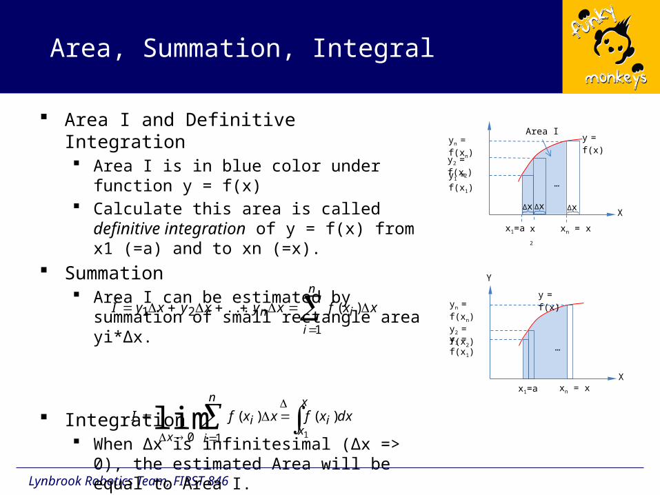
Area I and Definitive Integration Area I is in blue color under function y = f(x) Calculate this area is called definitive

integration of y = f(x) from x1 (=a) and to xn (=x).

Summation Area I can be estimated by summation of

small rectangle area yi*Δx.

Integration When Δx is infinitesimal (Δx => 0), the

estimated Area will be equal to Area I.

Area, Summation, Integral

x1=a xn = x

y1 = f(x1)

yn = f(xn)

X

Y

y = f(x)

…

y2 = f(x2)

Area I

x1=a xn = x

y1 = f(x1)

yn = f(xn)

X

y = f(x)

…

y2 = f(x2)

x2

Δx Δx Δx

n

i

in xxfxyxyxyI

1

21 )(...ˆ

x

xi

n

i

i

x

dxxfxxfI1

)()(

10lim


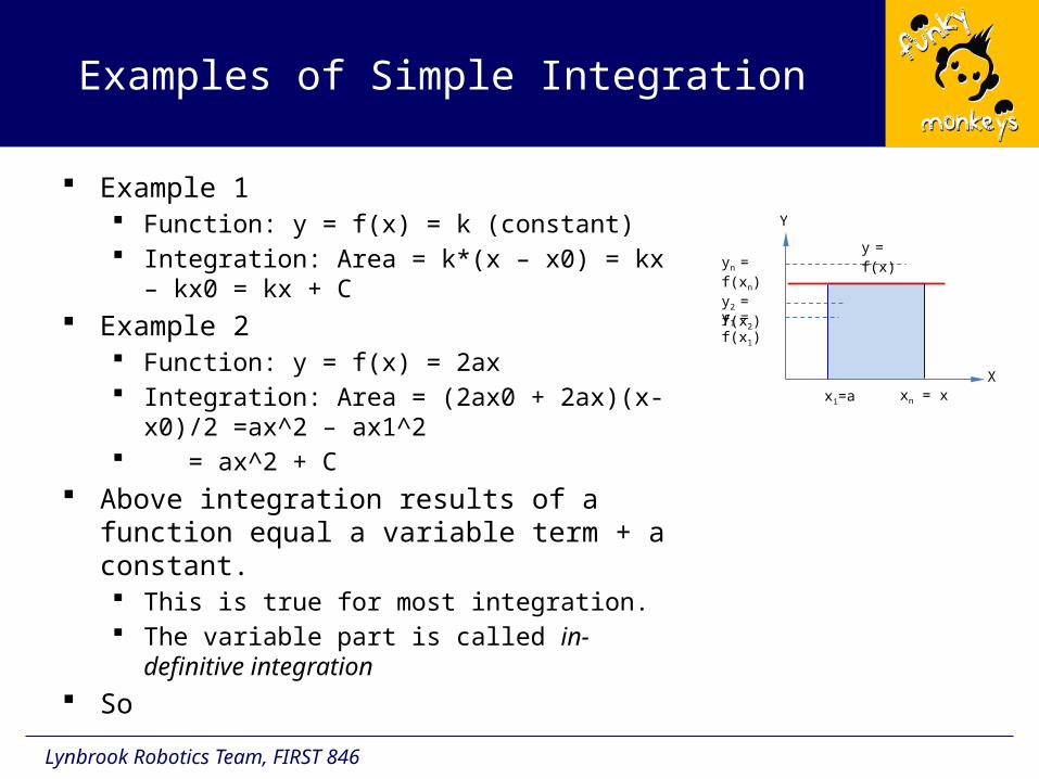
Example 1 Function: y = f(x) = k (constant) Integration: Area = k*(x – x0) = kx – kx0 = kx +

C Example 2

Function: y = f(x) = 2ax Integration: Area = (2ax0 + 2ax)(x-x0)/2 =ax^2

– ax1^2 = ax^2 + C

Above integration results of a function equal a variable term + a constant. This is true for most integration. The variable part is called in-definitive

integration So

Examples of Simple Integration

x1=a xn = x

y1 = f(x1)

yn = f(xn)

X

Y

y = f(x)

y2 = f(x2)


Relationship between Derivative and Indefinite Integration


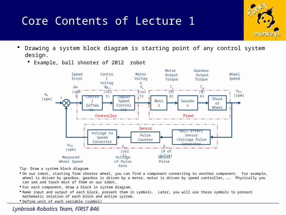
Drawing a system block diagram is starting point of any control system design. Example, ball shooter of 2012 robot

Core Contents of Lecture 1

Shooter Wheel

WheelSpeed

Hall Effect Sensor(Voltage Pulse

Generator

+

-

Speed Error

ω0

(rpm)GearboxMotor

JaguarSpeed

Controller

Control Software

Pulse CounterVoltage to

Speed Converter

Δω

(rpm)Vctrl

(volt)Vm

(volt)Tm

(N-m)Tgb

(N-m) ωwhl

(rpm)

Control Voltage

Motor Voltage

Motor Output Torque

Gearbox Output Torque

Voltage of Pulse Rate

Pwhl

(# of pulse)Vpls

(volt)

ωfbk

(rpm)

Sensor Pulse

Measured Wheel Speed

Controller Plant

Sensor

Tip: Draw a system block diagram On our robot, starting from shooter wheel, you can find a component connecting to another component. For example, wheel is driven by

gearbox, gearbox is driven by a motor, motor is driven by speed controller, …. Physically you can see and touch most of them on our robot. For each component, draw a block in system diagram. Name input and output of each block, present them in symbols. Later, you will use these symbols to present mathematic relation of each

block and entire system. Define unit of each variable (symbol)


To a step input (the red curve in following plots), responses of system with a well designed controller should have performance as the green curves. Green curves in both plots have optimal damping ratio (0.5 ~ 1) But, the green curve in right figure is preferred because it has faster response (higher bandwidth)


Systems with behavior as shown in above figures can be represented by 2nd order differential equation. 𝑋ሷ+ 2ζω𝑏𝑋ሶ+ 𝜔𝑏2𝑋= 𝐹(𝑡)

Tip: We take an approach to design our control system without solving this differential equation. Model robot system based on physics and mathematics. Typically we will get the 2nd order differential equation as above. Then we optimize

Damping ratio: ζ = 0.5 ~ 1. System bandwidth(close loop): ωb = 5 - 10 Hz for 50 Hz control system sampling rate


The characteristics of 2nd order differential equation (or a system which can be presented by the same equation)

can be examined by solving special cases such as F(t) = 0 or F(t) = 1 and given initial conditions. At this point, you can use solutions from Mr. G’s presentation for our robot control

system analysis and design.

Tip: use published solutions listed in table below for your simulation.


𝑋ሷ+ 2ζω𝑏𝑋ሶ+ 𝜔𝑏2𝑋= 𝐹(𝑡)

Damping Ratio

𝐹ሺ𝑡ሻ= 0, (Free Vibration) 𝑥ሺ𝑡 = 0ሻ= 𝑥0,𝑥ሶ(𝑡 = 0)𝑥ሶ0 𝐹ሺ𝑡ሻ= 1, (Step Input) 𝑥ሺ𝑡 = 0ሻ= 0,𝑥ሶሺ𝑡 = 0ሻ= 0

ζ< 1 𝑥ሺ𝑡ሻ= 𝑒−𝜁𝜔𝑏𝑡[𝑥0 cosඥ1− 𝜁2𝜔𝑏𝑡+𝑥ሶ0+𝜁𝜔𝑏𝑥0ඥ1−𝜁2𝜔𝑏 𝑠𝑖𝑛ඥ1− 𝜁2𝜔𝑏𝑡] 𝑥ሺ𝑡ሻ= 1− 𝜁𝑒−𝜁𝜔𝑏𝑡

ඥ1−𝜁2 𝑠𝑖𝑛ඥ1− 𝜁2𝜔𝑏𝑡−𝑒−𝜁𝜔𝑏𝑡 cosඥ1− 𝜁2𝜔𝑏𝑡 ζ = 1 𝑥ሺ𝑡ሻ= [𝑥0 +ሺ𝑥ሶ0 + 𝜔𝑏𝑥0ሻ𝑡]𝑒−𝜔𝑏𝑡 𝑥ሺ𝑡ሻ= 1− 𝑒−𝜔𝑏𝑡 − 𝜔𝑏𝑡𝑒−𝜔𝑏𝑡 ζ > 1 𝑥ሺ𝑡ሻ= 𝑒(−𝜁+ඥ𝜁2−1)𝜔𝑏𝑡 𝑥0𝜔𝑏ቀ𝜁+ඥ𝜁2−1ቁ+𝑥ሶሶ 02𝜔𝑏ඥ𝜁2−1 +

𝑒(−𝜁−ඥ𝜁2−1)𝜔𝑏𝑡 −𝑥0𝜔𝑏ቀ𝜁+ඥ𝜁2−1ቁ−𝑥ሶሶ 02𝜔𝑏ඥ𝜁2−1

𝑥ሺ𝑡ሻ= 1− 12൬ 𝜁ඥ𝜁2−1 + 1൰𝑒(−𝜁+ඥ𝜁2−1)𝜔𝑏𝑡 +

12൬ 𝜁ඥ𝜁2−1 − 1൰𝑒(−𝜁−ඥ𝜁2−1)𝜔𝑏𝑡


In rest of lectures we will get on real stuff of our robot. First, we will model ball shooter wheel, its gearbox and motor, etc. Second, analyze a proportional controller.

Proportion controller (P)with speed feedback is used on our shooter. Answer why the system is always stable (thinking about damping). Can step response be faster? Run step response test. Answer why this system can not keep constant speed in SVR. We will introduce disturbance

input in block diagram. Third, we will change the controller to proportion – integration controller (PI)

Analyze that under which condition this system will be stable or not stable. Program the controller on robot and see step response. Add load to shooter and see if speed can be constant.

Fourth, we will change the controller to proportion-integration-derivative (PID) controller if we can not achieve stable operation from above design. Modeling and analysis could be more complicated for students. But we will give a try. We will finalize the design and tune the system for CalGame.

Then, we will get on aiming position control system design for CalGame.

Heads-up

Lynbrook Robotics Team, FIRST 846 Control System Miniseries - Lecture 4 06/11/2012.

Documents

Transcript of Lynbrook Robotics Team, FIRST 846 Control System Miniseries - Lecture 4 06/11/2012.