Lyapunov Exponents and Strange Attractors in Discrete and

Continuous Dynamical Systems

Jo BovyJo.Bovy@student.kuleuven.ac.be

Theoretical Physics ProjectSeptember 11, 2004

Contents

1 Introduction 2

2 Overview 2

3 Discrete and continuous dynamical sys-tems 23.1 The Logistic Map . . . . . . . . . . . . 23.2 The Henon Map . . . . . . . . . . . . 33.3 The Lozi Map . . . . . . . . . . . . . . 43.4 The Zaslavskii Map . . . . . . . . . . . 43.5 The Lorenz System . . . . . . . . . . . 43.6 The Rossler System . . . . . . . . . . 5

4 Lyapunov Exponents 54.1 Definition and basic properties . . . . 64.2 Constraints on the Lyapunov exponents 74.3 Calculating the largest Lyapunov ex-

ponent - method 1 . . . . . . . . . . . 74.4 Calculating the largest Lyapunov ex-

ponent - method 2 . . . . . . . . . . . 84.4.1 Maps . . . . . . . . . . . . . . 84.4.2 Continuous systems . . . . . . 8

4.5 Calculating the other Lyapunov expo-nents . . . . . . . . . . . . . . . . . . . 9

4.6 Numerical Results . . . . . . . . . . . 9

5 Strange Attractors 125.1 Dimensions and definition of a strange

attractor . . . . . . . . . . . . . . . . . 125.1.1 Topological dimension . . . . . 12

5.1.2 Box-counting dimension . . . . 125.1.3 Correlation dimension . . . . . 135.1.4 Kaplan-Yorke dimension . . . . 135.1.5 Definition of a strange attractor 145.1.6 Concerning dimensions from

experimental data . . . . . . . 145.2 Algorithms for calculating dimensions 14

5.2.1 Box-counting dimension . . . . 145.2.2 Correlation dimension . . . . . 15

5.3 Results . . . . . . . . . . . . . . . . . . 15

6 Conclusion 17

A Oseledec’s multiplicative ergodic theo-rem 18A.1 The theorem . . . . . . . . . . . . . . 18A.2 A measure on the attractors . . . . . . 19

B Computer Programs 19

1

3 DISCRETE AND CONTINUOUS DYNAMICAL SYSTEMS 2

1 Introduction

Having already introduced a chaotic system (theLorenz system) in a previous paper [23] and hav-ing already studied chaos qualitatively in that paper,I will, in this paper, try to obtain some quantita-tive results concerning chaos. Therefor I will intro-duce some more dynamical systems, discrete systems(meaning they have discrete time steps) as well ascontinuous systems. Discrete systems are a lot eas-ier to handle than continuous systems. They can bechaotic even in less than two dimensions (which isprecluded for continuous systems by the Poincare-Bendixon theorem). And their solution doesn’t in-volve solving differential equations.

I will then study two aspects of these chaotic sys-tems. Firstly I will concentrate on measuring thechaos in the system. This is done by introducingLyapunov exponents, which measure the exponentialdivergence of nearby trajectories. When a Lyapunovexponents is positive, we will say that the system ischaotic.

All these systems also show a strange attractor forcertain parameter values. We will calculate the di-mensions of these attractors and see that the dimen-sions don’t have to be an integer. This fact is thereason why we call them strange.

2 Overview

Firstly I will describe some dynamical systems, bothdiscrete as continuous, and give their basic proper-ties. Then I will introduce the Lyapunov exponentsand give methods for their calculation. Next I shallmove on to strange attractors, give their definitionand explain how I used these definitions to write pro-grams that calculate their dimension.

3 Discrete and continuous dy-namical systems

The techniques for calculating Lyapunov exponentsand dimensions of strange attractors are not specificto the dynamical system under investigation. The

same algoritmes can be used on a large variety ofdynamical systems. Therefore I shall use the tech-niques that I develop later in this text not only onthe Lorenz system, but on a selection of the most im-portant and famous non-linear dynamical systems. Inthis section I will introduce these dynamical systemsand list there basic properties. I begin by describingsome discrete systems, i.e. two-dimensional maps. Iwill also introduce a second three-dimensional con-tinuous dynamical system in addition to the Lorenzsystem: the Rossler system.

3.1 The Logistic Map

The Logistic map is obtained by replacing the Logis-tic equation for population growth with a quadraticrecurrence relation. This model was first publishedby Pierre Verhulst [27, 28].

The Logistic equation is

dx

dt= rx(1− x) (1)

The Logistic map is given by

xn+1 = rxn(1− xn) (2)

with r a positive constant sometimes known as the“biotic potential”.

We can understand this equation as follows [5]: as-suming constant conditions every year, the popula-tion (of insects for example) at year n uniquely deter-mines the population at year n+1. Therefor we havea one-dimensional map. Say that there are zn insectsat year n and that every insect lays, on the average, reggs, each of which hatches at year n+1. This wouldyield a population at year n+1 of zn+1 = rzn. Whenr > 1, this yields an exponentially increasing popula-tion. When the population is too large however, theinsects will exhaust there food supply as they eat andgrow, and not all insects will reach maturity. Hencethe average number of eggs laid will become less thanr as zn is increased. A simple assumption is then thatthe number of eggs laid per insect decreases linearlywith the insect population, r[1 − (zn/z)], where zis the population at which the insects exhaust theirfood supply. We then have the one-dimensional map

3 DISCRETE AND CONTINUOUS DYNAMICAL SYSTEMS 3

zn+1 = rzn[1− (zn/z)]. Dividing both sides by z andletting x = z/z, we obtain the Logistic map (2).

In general, this equation cannot be solved in closedform and it is capable of very complicated behavior.Many aspects of this equation and it’s chaotic be-havior can however be studied exactly. We’ll taker ∈ [0, 4] to keep all xn in the interval [0, 1] [10]. TheJacobian is

J =∣∣∣∣dxn+1

dxn

∣∣∣∣ =| r(1− 2xn) | (3)

The map is stable at a point x0 if J(x0) < 1.To find the fixed points of the map we have to

solve the equation (dropping the subscripts on x forconvenience)

x = rx(1− x) (4)

so the fixed points are x(1)1 = 0 and x

(1)2 = 1− 1

r . TheJacobian evaluated at these points gives is

J(x(1)1 ) =| r | (5)

J(x(1)2 ) =| 2− r | (6)

so the first fixed point is stable until r = 1, whereit becomes unstable. The second fixed point is un-stable for r < 1 and stable for 1 < r < 3. Atr = 3 both fixed points are unstable. At this valuefor r period doubling occurs. The system begins aperiod-doubling route to chaos that is completed atr = 3.5699456. At this value the system becomeschaotic. This is the value we will use to calculate theLyapunov exponent and dimension of the strange at-tractor that occurs.

3.2 The Henon Map

Henon introduced this map as a simplified versionof the Poincare map of the Lorenz system [25]. ThePoincare map of a system is the map which relatesthe coordinates of one point at which the trajectorycrosses a Poincare plane to the coordinate of the next(in time) crossing point. The existence of this map isassumed to be the consequence of the uniqueness ofthe solution of the equation of the dynamical system.

The Henon equations are

xn+1 = 1− ax2n + yn (7)

yn+1 = bxn (8)

This map is invertible, with the inverted map givenby

xn =yn+1

b(9)

yn = xn+1 − 1 + ay2

n+1

b2(10)

This makes the calculation of basins of attractionmuch simpler. We shall however not look at thesebasins of attraction (see for instance [8, 14]).

The Jacobian matrix J of the Henon map is(−2ax 1

b 0

)The determinant of this Jacobian is b. By a basicresult of linear algebra, the factor by which an areagrows under a linear transformation is given by theabsolute value of the determinant of the matrix repre-senting the transformation. Locally we can linearizethe Henon transformation, so a small area near apoint P = (x, y) is reduced by the factor given bythe absolute value of the determinant of the deriva-tive (the Jacobian matrix) of the transformation atthat point. This gives |det(J)| = |b|, a constant value,not dependent on the location of P .

The fixed points of the Henon map are

(x, y) =−1 + b±

√1− 2b + b2 + 4a

2a(1, b) (11)

When we calculate the eigenvalues of the Jacobianmatrix J , we can see when these fixed points are sta-ble. The eigenvalues are

λ(1,2) = −ax±√

a2x2 + b (12)

For a = 1.4 and b = 0.3 (the values for which theHenon map has a strange attractor), these eigenval-

3 DISCRETE AND CONTINUOUS DYNAMICAL SYSTEMS 4

ues for the fixed points are

λ(1)1 = −0.092029562

λ(1)2 = 0.6915136742

λ(2)1 = −0.8079567198

λ(2)2 = 0.1559463222

so both fixed points are not-stable.

3.3 The Lozi Map

The Lozi map is a simplification of the Henon map.The quadratic term in xn (−ax2

n) is replaced by−a|xn|. The Lozi map is then given by

xn+1 = 1− a|xn|+ yn (13)yn+1 = bxn (14)

We can write the Jacobian matrix using the Heav-iside step-function

Θ(x) ={

0 x < 01 x ≥ 0 (15)

The Jacobian J then becomes(−a

(2Θ(x)− 1

)1

b 0

)The determinant is still b.

This map has a strange attractor we shall studyfor the parameter values a = 1.7, b = 0.5. The fixedpoints for these parameter values are

(x, y)1 = (511

,522

) (16)

(x, y)2 = (−56

,−512

) (17)

The eigenvalues of the Jacobian matrix are

λ(1,2) =−a

(2Θ(x)− 1

)±√

a2 + 4b

2(18)

and the eigenvalues evaluated at the fixed points

(again a = 1.7, b = 0.5) are

λ(1)1 =

−1720

−√

48920

= −1.95566722

λ(1)2 =

−1720

+√

48920

= 0.25566722

λ(2)1 =

1720−√

48920

= −0.25566722

λ(2)2 =

1720−√

48920

= 1.95566722

so both points are not-stable.

3.4 The Zaslavskii Map

The Zaslavksii map [13] is given by the followingequations

xn+1 = xn + ν + ayn+1(mod1) (19)

yn+1 = cos(2πxn) + e−ryn (20)

To compute the Jacobian, we write the equationsas follows

xn+1 = xn + ν + a(cos(2πxn) + e−ryn

)(mod1)

(21)

yn+1 = cos(2πxn) + e−ryn (22)

The Jacobian is then(1− 2πa sin(2πxn) ae−r

−2π sin(2πxn) e−r

)The determinant is equal to e−r, so areas shrink bya factor of e−r every iteration (r > 0).

The Zaslavskii map shows a strange attractor forν = 400, r = 3, a = 12.6695.

3.5 The Lorenz System

I have already studied the Lorenz system [7] exten-sively in a previous project [23]. I studied the basicproperties of the Lorenz system (fixed points, stabil-ity and basins of attraction). So the reader shouldconsult this for an overview of the basic properties.

4 LYAPUNOV EXPONENTS 5

Other good references are [15, 31]. I will just statethe Lorenz equations

X = p(Y −X)

Y = rX −XZ − Y

Z = XY − bZ

(23)

I shall study the Lorenz strange attractor for theparameter values p = 10, b = 8/3, r = 28.

3.6 The Rossler System

The Rossler system [26] is one of the most simplechaotic continuous systems. It is artificially designedsolely with the purpose of creating a simple model fora chaotic strange attractor. The system of differentialequations is

x = −(y + z) (24)y = x + ay (25)z = b + xz − cz (26)

with a,b and c adjustable paramters of which a andb are usely fixed at a = 0.2, b = 0.2. This system isobviously simpler than the Lorenz system, because itcontains only one non-linear term. It is however notthe simplest chaotic flow, since the simplest dissipa-tive flow has been argued to be

...x+Ax−x2+x = 0 [17]

(This equation can easily be converted to a system offirst order differential equations using the followingsubstitutions: x = y, x = z).

The divergence of the flow, ∇·f (writing the systemas y = f) = ∂x

∂x + ∂y∂y + ∂z

∂z = a+x− c. Note that thisis not a constant, hence the shrinking/expansion ofvolumes is not uniform over phase space.

The fixed points are

(x, y, z) =c±

√c2 − 4ab

2a(a,−1, 1) (27)

The Jacobian matrix is 0 −1 −11 a 0z 0 x− c

Setting the parameter c = 5.7 (we shall study thestrange attractor that occurs at this parameter value)the eigenvalues are

λ1 = 0.0970008560175134871 + i0.995193491034748634λ2 = 0.0970008560175134871− i0.995193491034748634λ3 = −5.68697550703502762

and

λ1 = −0.459615167119897806e− 5 + i5.42802593149083901λ2 = −0.459615167119897806e− 5− i5.42802593149083901λ3 = 0.192982987303353531

so both fixed points are not-stable.

4 Lyapunov Exponents

As with everything else in Physics, and especially inTheoretical Physics, we don’t content ourselves withjust a qualitative picture of chaos. In this sectionI’ll introduce a quantitative measure of chaos, thecelebrated Lyapunov Exponents.

Introducing a quantitative measure of chaos is im-portant for several reasons. Most importantly it al-lows us to define exactly what we mean by chaos.When we only have a qualitative picture of chaos,everybody has a different opinion of what chaos is.One just looks for instance at the picture in phasespace and decides wether or not he finds it chaotic.Science would not have come as far as it is now ifwe had contented ourselves with such qualitative pic-tures. So introducing a measure of chaos allows us torigourously define what we mean by chaos.

Having this measure of chaos allows us to go fur-ther and compare different systems. We can definewhat we mean by saying that one system is morechaotic than another system. Thus we can comparethe chaoticness of a system with different parametervalues, or the chaoticness of two completely differentsystems.

In the first subsection of this section I will defineand discuss the Lyapunov exponents. In the nextsubsections I will discuss how I calculated the Lya-punov exponents and state the results I got for themaps described in the previous section.

4 LYAPUNOV EXPONENTS 6

4.1 Definition and basic properties

Since we want to measure chaotic behavior, which weintuitively defined as sensitivity on initial conditions,we shall look at the evolution of a small displacementof a initial condition x0 (with corresponding orbit xn

n = 0, 1, 2, . . .). First take a map M. If we consideran infinitesimal displacement from x0 in the directionof a tangent vector y0, the evolution of the tangentvector, given by

yn+1 = DM(xn) · yn (28)

determines the evolution of the infinitesimal displace-ment of the orbit from the unperturbed orbit xn

(DM is just the Jacobian matrix). So |yn|/|y0| is thefactor by which the infinitesimal displacement growsor shrinks. From (28) we have yn = DMn(x0) · y0,where DMn(x0) = DM(xn−1) · DM(xn−2) · . . . ·DM(x0). We then define the Lyapunov exponent1

for initial condition x0 and initial orientation of theinfinitesimal displacement given by u0 = y0/|y0| as

λ(x0,u0) = limn→∞

1n

ln(|yn|/|y0|)

= limn→∞

1n

ln|DMn(x0) · u0|(29)

Note that these exponents are (for now) dependenton the initial condition.

If the dimension of the map is N , then there willbe N Lyapunov exponents, since there are N inde-pendent initial displacement directions. Since

λ(x0,u0) u λn(x0,u0) ≡1n

ln|DMn(x0) · u0|

=12n

ln|u†0 ·Hn(x0) · u0|(30)

where Hn = [DMn]†DMn, and † denotes thetranspose, we get N eigenvalues of Hn (Hjn) eachcorresponding to one Lyapunov exponent (λjn =(2n)−1 lnHjn). Every initial displacement u0 can be

1In the literature one encounters often reference to Lya-punov numbers µ. These are given in terms of the Lyapunovexponents λ by µ = exp(λ).

decomposed in the orthonormal eigenvectors ej of Hn

u0 =n∑

j=1

ajej (31)

and the Lyapunov exponent of such an initial dis-placement can be written in function of the eigenval-ues of Hn(x0), since

u†0 ·Hn(x0) · u0 =n∑

j=1

a2j exp[2nλjn(x0)] (32)

An important question now is wether the limitsin (29) exist. This existence is guaranteed by Os-eledec’s multiplicative ergodic theorem under verygeneral circumstances. This theorem is stated in ap-pendix A with some of its consequences. One of itsconsequences is that the Lyapunov exponents are thesame for almost every x0 with respect to the natu-ral measure on the attractor (this natural measure isalso described in appendix A).

Now I will move on to define Lyapunov exponentsin continuous time systems. All the above consider-ations remain valid when we replace Eq. (29) by

λ(x0,u0) = limn→∞

1n

ln(|yn|/|y0|)

= limn→∞

1n

ln|O(x0, t) · u0|(33)

where dy(t)dt = F(x(t)) · y(t), x0 = x(0), y0 = y(0),

u0 = y(0)/|y(0)|, and O(x0, t) is the matrix solutionof the equation

dO/dt = DF(x(t)) ·O (34)

with initial condition

O(x0, 0) = I

This equation is called the variational equation. Tocalculate the Lyapunov exponents we’ll have to solvean additional system of differential equations.

Now that we have defined Lyapunov exponents, wecan define what we mean by saying that a system ischaotic. We say that a system is chaotic when ithas at least one strictly positive Lyapunov exponent.

4 LYAPUNOV EXPONENTS 7

When a system has a positive Lyapunov exponent,small disturbances will give rise to exponential diver-gence. So this definition is in accordance with thequalitative picture we had.

Now how can we represent what these differentLyapunov exponents mean. When we consider asmall ball (say infinitesimal, radius dr) of initialconditions around an initial condition x0, and thenevolve every initial condition inside this ball for n it-erates. The ball will have evolved into an ellipsoid. In the limit of large time the Lyapunov exponentsgive the time rate of exponential growth or shrinkingof the principal axes of the evolving ellipsoid. Theaxes will be (approximately) given by the expressionsa1 = exp(nλ1)dr and a2 = exp(nλ2)dr.

4.2 Constraints on the Lyapunov ex-ponents

We can deduce some constraints on the Lyapunovexponents of a dynamical system. Using these con-straints we should only calculate the largest Lya-punov exponent for all but one of the dynamical sys-tems I described in section 3. I shall however in thefollowing sections calculate all Lyapunov exponentsand use them to check the validity of these relations.

In systems where the area-reducing factor (or vol-ume reducing factor in three dimensional systems) isconstant, we can derive a relation between the Lya-punov exponents. Since exp(

∑i λi) is equal to the

area-reduction, this must be equal to the determi-nant of the Jacobian (for maps) or to exp(∇· f) (∇· fis the divergence of the flow for continuous dynamicalsystems).

Applying this to the Henon system, we see thatλ1 +λ2 = ln(|b|). We could only calculate the largestexponent and derive the second from this relation.

For a continuous dynamical system we can look atdisturbances in the direction of the velocity vectorof the trajectory (see page 718 in [14]). Consider atrajectory (x(t), y(t), z(t)) and a perturbed trajectory(x(t), y(t), z(t)) with initial condition

x(0) = x(δ), y(0) = y(δ), z(0) = z(δ)

with δ > 0. So the trajectory starts on the referencetrajectory, and, if we assume the system to be au-

tonomous, it will follow the same trajectory as thenot-disturbed trajectory. These trajectories clearlydo not diverge from each other, on the average theywill keep at the same distance of each other. So inthis direction the Lyapunov exponent is zero. So inevery continuous dynamical system one of the Lya-punov exponents will be zero (except for systems witha fixed point).

Applying this to the Lorenz system, which has aconstant divergence equal to −(1 + b + p), we havethe following two relations

λ1 + λ2 + λ3 = −(1 + b + p) (35)λ2 = 0 (36)

so again we could only calculate the largest Lyapunovexponent (λ1), and deduce the other two from thesetwo relations. We can’t use this on the Rossler systemhowever because its divergence isn’t a constant.

4.3 Calculating the largest Lyapunovexponent - method 1

As pointed out in appendix A, the largest Lyapunovexponent is the easiest one to calculate. If we startby choosing a direction vector randomly, we can de-compose it as in (31). It will most probably havea non-zero component in the direction of the eigen-vector of the largest exponent. Since in the caseswe consider only one Lyapunov exponent is positive,evolution will be dominated by the largest exponent,as seen from (32).

We can then calculate this exponent by juststraightforwardly using our qualitative understand-ing (in the next subsection I will give a better methodbased on the differential map). We have to calculate

λ1 = limn→∞

limE0→0

1n

ln(|En|/|E0|) (37)

with E0 an initial disturbance. We can write

|En||E0|

=|En||En−1|

|En−1||En−2|

· · · |E1||E0|

(38)

substituting (38) in (37), we get

λ1 = limn→∞

limE0→0

1n

n∑k=1

ln(|Ek||Ek−1|

) (39)

4 LYAPUNOV EXPONENTS 8

We will however in our algorithm renormalize ourerror to some chosen value ε. For one-dimensionalmaps such as the Logistic map, we essentially haven’tgot any choice of direction of the error. For two-or three-dimensional systems we have to choose thedirection of the error. For two-dimensional maps we’lldefine an error of size ε on (x, y)

(x, y) = (x + ε cos φ, y + ε sinφ) (40)

with φ an arbitrary angle. For three-dimensional sys-tems this becomes on (x, y, x)

(x, y, z) = (x+ε sinφ cos σ, y+ε sinφ sinσ, z+ε cos φ)(41)

The algorithm2 now works as follows (it is de-scribed for maps, but it is easily adjusted to con-tinuous systems):

1. We choose an initial point an let the map iteratethis for say 100 times. We do this to let tran-sients die out.

2. We compute the perturbed point according to(40) or (41).

3. We iterate both points and compute the distanced between them

4. We add log d/ε to an accumulator

5. We renormalize the error

6. We iterate steps 3-5

7. The result is the average of the log di/ε, thus theaccumulator divide by the number of iterations

4.4 Calculating the largest Lyapunovexponent - method 2

The program outlined in the previous subsection isn’tquite accurate, because we should actually take thelimit ε → 0. We can take this limit by consideringthe differential map.

2this algorithm and the ones in the following section arewritten along the lines given in [14] pg.710

4.4.1 Maps

For maps this is not such a hard task. We just cal-culate the Jacobian matrix, and this gives us the dif-ferential map. This map tells us how an infinitesimalsmall error gets amplified. The algorithm is then asfollows

1. We choose an initial point an let the map iteratethis for say 100 times. We do this to let tran-sients die out.

2. We consider for an arbitrary angle φ the direc-tion (cos φ, sinφ) (generalizing this to three di-mensions is obvious).

3. We compute the next point of the map H(x, y)and the transformed error E(x, y) using the dif-ferential map. So we get the point E(x, y) =DM(x, y) · (cos φ, sinφ)†.

4. The error has increased by d = ‖E(x, y)‖. Weadd log d to an accumulator.

5. We renormalize the direction vector to a unitvector (E′(x, y) = E(x, y)/d). Then we go backto step 3 using the new point and the new error.

6. The result is once again the accumulator dividedby the number of iterations.

4.4.2 Continuous systems

The algorithm is essentially the same as the one de-scribed in the previous section. We only have to ad-just the manner of computing the transformed direc-tion vector. To find this transformed direction vec-tor, we have to solve the variational equation. Alsoin continuous systems, we have to choose the timeinterval over which each iteration reaches. When weconsider discrete maps, we have always iterated themap one discrete time step. When considering con-tinuous maps we choose to let the system evolve forone timestep (such that tn+1 = tn + 1). So when wechoose an integration step of 1/N in our numericalsolver, we have iterate this for N times. After theseN times we look at our new direction vector, andmeasure its amplification.

4 LYAPUNOV EXPONENTS 9

4.5 Calculating the other Lyapunovexponents

Because of theorem 2 in appendix A.1, when calcu-lating the second (or third or higher) Lyapunov expo-nent, we should start with a vector that is orthogonalto the eigenvector of the first Lyapunov exponent (orin the case of higher Lyapunov exponents, we shouldstart with a vector orthogonal to all eigenvectors, be-longing to the Lyapunov exponents bigger than theone we want to calculate). This is however not aneasy task. For continuous systems, which we have tosolve numerically, the situation is even worse becausedue to numerical integration errors, components fromthe eigenvector of the largest Lyapunov exponent willbecome not-zero, and dominate the further evolution.

So we have to think of another way of calculatingthe remaining Lyapunov exponents. I will give thedescription of this method for the second Lyapunovexponent, but one can easily see from this expositionhow the algorithm works for arbitrary Lyapunov ex-ponents. The idea is to compute not the second Lya-punov exponent, but the sum of the first and secondLyapunov exponent, and then compute the secondout of our knowledge of the first (for the third for in-stance we shall have to compute the sum of the firstthree exponents and then calculate the third from ourknowledge of the first and the second).

How are we going to calculate the sum of the firstand second exponent? By looking at the evolutionof two orthonormal error directions, and look at theamplification of the area they span (we shall immedi-ately use the differential map to calculate the trans-formed errors). When assuming that the original vec-tors have components in the directions of the eigen-vectors of the first and the second eigenvalue, thearea will behave as An ≈ exp[n(λ1 + λ2)]A0 (whenthe vectors also have components in the direction ofthe other eigenvectors, the largest two will dominatethe growth). Thus we have

λ1 + λ2 = limn→∞

1n

ln(An/A0) (42)

So the algorithm doesn’t change much. We have tocalculate two transformed directions, and the areathat they span will be the amplification factor. We

have to be careful about the renormalization how-ever. Because the first Lyapunov is the largest, thearea will shrink very quickly, and the parallellogramspanned will become more and more a line in the di-rection of the first eigenvector. Thus we shall renor-malize the two transformed vectors by Gram-Schmidtorthogonalization, so that they once again form a or-thonormal pair.

I shall give an overview of the algorithm I used fora two-dimensional map

1. We choose an initial point an let the map iteratethis for say 100 times. We do this to let tran-sients die out.

2. We consider for an arbitrary angle φ thedirection (cos φ, sinφ) and the direction(− sinφ, cos φ) (generalizing this to threedimensions is obvious).

3. We compute the next point of the map H(x, y)and the transformed errors E1(x, y), E2(x, y)using the differential map. So we get thepoints E1(x, y) = DM(x, y) · (cos φ, sinφ)† andE2(x, y) = DM(x, y) · (− sinφ, cos φ)†.

4. The area has increased/shrunk by d =det |E1(x, y) E2(x, y)|. We add log d to an ac-cumulator.

5. We renormalize the directions using Gram-Schmidt orthogonalization. Then we go back tostep 3 using the new point and the new errors.

6. The result is once again the accumulator dividedby the number of iterations.

The adjustments necessary for continuous systemsshould be clear.

4.6 Numerical Results

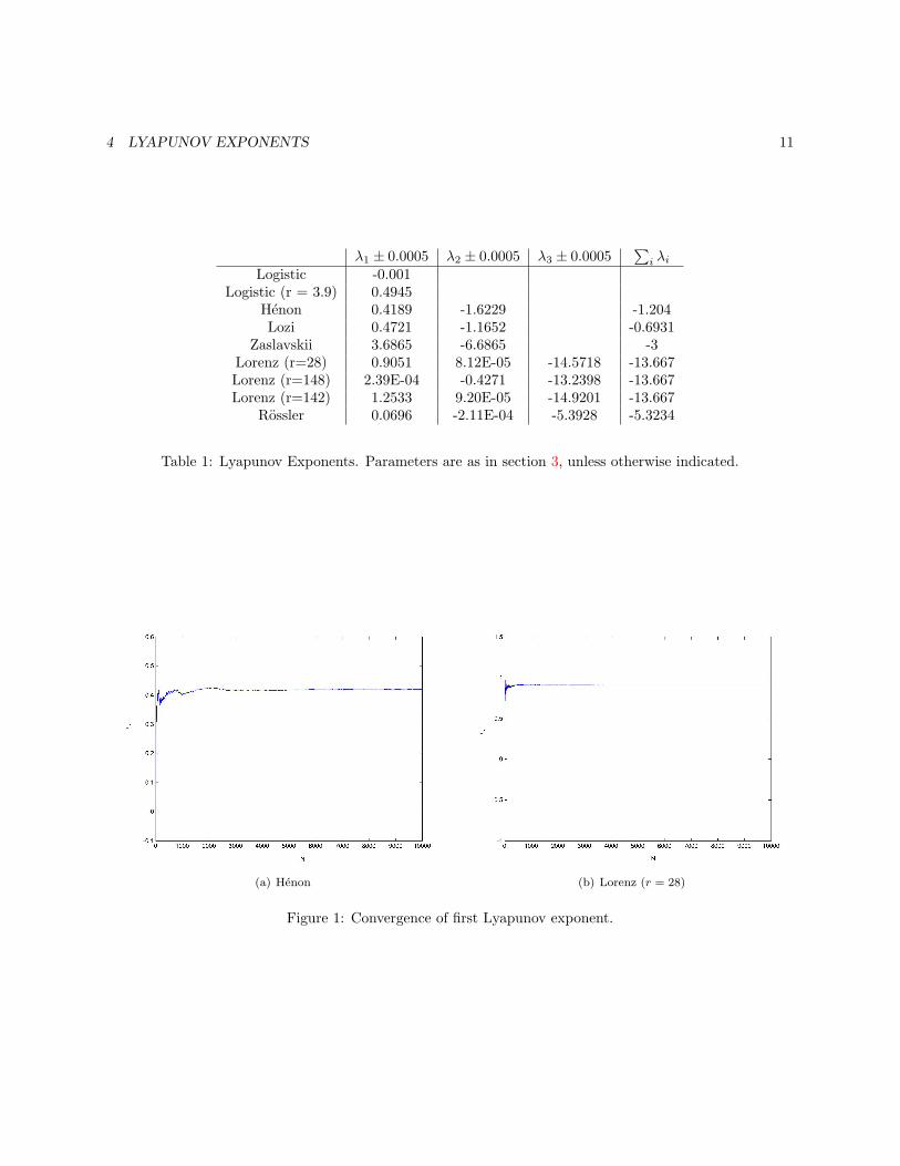
I calculated all Lyapunov exponents of the systemsfrom section 3 using 10000 iterations and using thedifferential map method. The results are stated intable 1. I have also included graphs showing theconvergence towards the Lyapunov exponent for thelargest Lyapunov exponent of the Henon system and

4 LYAPUNOV EXPONENTS 10

the Lorenz system. In both cases we see that theconvergence is very quick.

We immediately see that all results are in agree-ment with the relations we discussed in section 4.2.The small deviations on the exponents that should bezero (for instance for the Lorenz system) can actuallybe used to estimate the error we make in calculatingthe Lyapunov exponents. So using this and taking inconsideration the fluctuations we see when we zoomin on the convergence-figure 1, I would estimate theerror for the Lorenz system to be ±0.0005. For theRossler system the error will be of the same magni-tude. And since we don’t make numerical integrationerrors in the two-dimensional maps, we expect thevalue for the Lorenz system to be an upper bound onthe error of the two-dimensional maps. So I shall usethis value for all systems.

I will now shortly comment on the individual re-sults.

Logistic map The Logistic map is not chaotic forthe parameter value r = 3.5699456. We see that it ison the verge of getting chaotic and this is in agree-ment with the value one finds at which the period-doubling ends. Setting r = 3.9, we see that for thisvalue the Logistic map is chaotic.

Henon map We see that the Henon map is chaotic.The sum of its two Lyapunov exponents (−1.204) isin very good agreement with its area reducing factor(0.3, we should take the logarithm of this numberin order to get the sum of the exponents, ln 0.3 =−1.20397).

Lozi map The Lozi map is also chaotic, and itis even more chaotic than the Henon map. Thesum of its Lyapunov exponents (-0.6931) is in verygood agreement with its theoretical value (ln 0.5 =−0.693147).

Zaslavskii map The Zaslavskii map is very chaotic(largest Lyapunov exponent 3.6865). The sum of theLyapunov exponents should equal the parameter r,and it does so very nicely.

Lorenz system The Lorenz system is chaotic fortwo of the parameter values I studied. For r = 148 itis not chaotic. In my previous project [23] we sawthat the Lorenz system has a periodical attractorat this parameter value. The calculated Lyapunovexponents confirm this : the largest is zero for thesame reason as stated in section 4.2, along the pe-riodical orbit there is on the average no divergenceor convergence of nearby trajectories, so one of theexponents has to be zero. Only when we have afixed point, none of the exponents will be zero. Sothis orbit must be a periodical orbit (since we haveonly three possibilities: fixed point, periodical or-bit or chaotic attractor). In all three cases understudy the three Lyapunov exponents add up nicelyto −(1 + p + b) = −41/3 = −13.6666 . . ..

Rossler system We see that the Rossler systemis only slightly chaotic. Adding the Lyapunov expo-nents has no use, since the divergence of the flow isn’ta constant. The sum however does agree nicely withthe average of the divergence over the attractor.

4 LYAPUNOV EXPONENTS 11

λ1 ± 0.0005 λ2 ± 0.0005 λ3 ± 0.0005∑

i λi

Logistic -0.001Logistic (r = 3.9) 0.4945

Henon 0.4189 -1.6229 -1.204Lozi 0.4721 -1.1652 -0.6931

Zaslavskii 3.6865 -6.6865 -3Lorenz (r=28) 0.9051 8.12E-05 -14.5718 -13.667Lorenz (r=148) 2.39E-04 -0.4271 -13.2398 -13.667Lorenz (r=142) 1.2533 9.20E-05 -14.9201 -13.667

Rossler 0.0696 -2.11E-04 -5.3928 -5.3234

Table 1: Lyapunov Exponents. Parameters are as in section 3, unless otherwise indicated.

(a) Henon (b) Lorenz (r = 28)

Figure 1: Convergence of first Lyapunov exponent.

5 STRANGE ATTRACTORS 12

5 Strange Attractors

The systems described in section 3 all show a strangeattractor for certain parameter values. I will definewhat a strange attractor is in the next subsection. Ininvestigating the properties of these strange attrac-tors, I will focus on their dimension. We shall shortlysee that dimension is a broader notion then one mightthink. The dimension doesn’t have to be an integerfor example.

Now what is the meaning of the dimension of astrange attractor? In a dissipative system, almostall initial values will eventually settle on an attrac-tor. When we know the dimension of this attrac-tor, we could say that the degrees of freedom thedynamical system has, is essentially this dimension,and this could be significantly less than the dimen-sion of the underlying phase space. In the systemsunder study here this isn’t very spectacular (two-dimensional phase space with 1.5-dimensional attrac-tor for example), but we must not forget that thesesystems are idealizations which don’t occur in reallife. Processes in real life can for example be de-scribed by a system of partial differential equations,which typically has a infinite number of degrees offreedom. When we see that these systems exhibit afinite-dimensional strange attractor, we can look fora small set of variables which describe the system inits attractor state. Also in experimental situations,one often doesn’t know the dimension of the phasespace he’s working in, since one doesn’t know exactlyall the variables contributing to a phenomenon. Sothe dimension of the strange attractor a experimentalsystem may show, is the only thing one knows aboutthe degrees of freedom of the system.

For all these reasons, strange attractors have madetheir way into the whole off the scientific world. Theyare used to describe a large variety of systems, forexample in immunology [32] or biology [30].

Firstly I shall give some explanation on the dimen-sions involved and then use these dimensions to definea strange attractor. Then I will describe how I usedthese definitions to calculate the dimensions of thesystems under study and state my results.

5.1 Dimensions and definition of astrange attractor

5.1.1 Topological dimension

The dimension we are all familiar with is called thetopological dimension. A set of disconnected points(by this I mean that they are not infinitely close to-gether as on a line, which is also just a set of points)has dimension zero. Curves have dimension one, sur-faces have dimension two. The topological dimensionof an object is always an integer. As a non-trivial ex-ample I mention the Cantor set (which one gets bydividing the unit interval in three equal pieces, throw-ing away the middle piece and iterate this procedureon the two remaining pieces). This set is just a set ofpoints (however uncountable) and thus has a topo-logical dimension zero.

5.1.2 Box-counting dimension

One can define for every object something called itsHausdorff-Besicovitch dimension. The definition ofthis dimension is however rather intricate. It can befound in the appendix of [1]. For most systems itcoincides with the Box-counting dimension. This di-mension is defined as follows: Consider ’boxes’ (inone dimension this would be intervals, in two dimen-sions squares, in three dimensions cubes, and so on)of side R, then cover the object with these boxes, andthen we count the number N(R) of boxes necessaryto contain all points of the object. As we let thesize of these boxes get smaller, we expect the N(R)to increase. The box-counting is then defined as thenumber Df that satisfies

N(R) = limR→0

kR−Df (43)

where k is a proportionality constant. We find Db

thus by taking the logarithm of both sides, beforetaking the limit

Df = limR→0

{− log N(R)

log R+

log k

log R

}(44)

Since k is a constant the last term will go to zero,when R goes to zero, so actually we have

Df = − limR→0

log N(R)log R

(45)

5 STRANGE ATTRACTORS 13

In practice we shall verify this law (43) by comput-ing N(R) for an appropriate scaling region, and thenplotting − log N(R) against log R. By using linearregression we can see how well this law is satisfiedand the Df is then given by the slope of the fittedline.

Is this a good definition for a dimension? Well it iseasy to see that for all Euclidean objects (a point, aline, a plane, . . .) it just gives the topological dimen-sion. I.e. we always need one box to cover a point, sothe limit (45) will be zero. In case of a line segmentof length L we need N(R) = L/R boxes to cover it.So the limit will be one.

Consider however the set { 1n}

∞n=2. This is just a

countable set of disconnected points, so one wouldexpect its dimension to be zero. However, I cal-culated the box-counting dimension in the followingway. Consider intervals of length 1

R(R−1) . This rep-resents the distance between the points 1

R and 1R−1 .

All points 1i for which i < R will be separated from

each other by an amount greater than 1R(R−1) . So we

need for each of these points an individual interval.This gives us already R − 2 intervals. To cover theremaining points we need 1/R

1/R(R−1) = R−1 intervals.Thus N(R) = 2R− 3 and we get

Df = − limR→0

log N(R)log 1

R(R−1)

= limR→0

log 2R− 3log R(R− 1)

=12

(46)which obviously isn’t zero. So this can be re-garded as a failure of the definition of the box-counting dimension. It can be shown however thatthe Hausdorff-Besicovitch dimension of this set iszero. So the Hausdorff-Besicovitch dimension hasn’tgot this problem.

5.1.3 Correlation dimension

The box-counting dimension, however relatively easyto understand, isn’t easy to calculate. In higher di-mensional spaces there is so much more space, so weneed much more boxes, and thus much more pointson our attractor, which are mostly calculated by acomputer or come from experimental data. And cal-culating these points can take a lot of time. So in

1982 Grassberger and Procaccia suggested a new wayto define a dimension [29].

Start with a long-time series on the attractor{~Xi} N

i=1 ≡ {~X(t + iτ)} Ni=1 where τ is an arbitrary

but fixed time increment. We then define the corre-lation to be

C(r) = limN→∞

1N(N − 1)

N∑i,j=1 i 6=j

Θ(r − |~Xi − ~Xj |)

(47)where Θ is the Heaviside function as defined in (15)and we use for example the Euclidean norm (onecould also take the maximum norm to speed up thecalculations). We then assume that for small r C(r)behaves as follows

C(r) ∝ rDc (48)

Dc is then called the correlation dimension. We cal-culate it using the same procedure as in the previoussubsection, choosing an appropriate scaling intervaland fitting a line on the plot of log C(r) against log r.

This dimension is sensitive to the distribution ofthe points on the attractor, since crowded regions willyield an higher correlation. When the distribution ofpoints on the attractor is uniform, the correlationdimension equals the box-counting dimension. Oth-erwise it is smaller. We could compare box-countingand correlation dimension with average and variancein statistics, the average also doesn’t care much aboutthe distribution of the values3.

5.1.4 Kaplan-Yorke dimension

Kaplan and Yorke proposed a dimension based onthe Lyapunov exponents of the system. Let us rankthe Lyapunov exponents from the largest λ1 to thesmallest λd. Let j be the largest integer such thatλ1 +λ2 + . . .+λj > 0, then the Kaplan-Yorke dimen-

3actually we should compare the correlation dimension withthe second moment, since the first moment, the variance instatistics, can be compared with yet another dimension, theinformation dimension. This dimension is part of a bunchof generalized dimensions which can be compared with thearbitrary moments of a distribution in statistics.

5 STRANGE ATTRACTORS 14

sion is defined to be

DKY = j +∑j

i=1 λi

−λj+1(49)

Kaplan and Yorke conjectured that, for a two-dimensional mapping, the box-counting dimensionDf equals the Kaplan-Yorke dimension DKY [24].This was subsequently proven to be true in 1982. Alater conjecture held that the Kaplan-Yorke dimen-sion is generically equal to another dimension calledthe information dimension, which is also closely re-lated to the box-counting dimension and the correla-tion dimension. This conjecture is partially verifiedby Ledrappier (1981). (This paragraph partially from[9]).

5.1.5 Definition of a strange attractor

We can now define what we mean by a strange attrac-tor. We shall say that an attractor is strange whenits Hausdorff dimension strictly exceeds the topolog-ical dimension [1] (in dynamical systems we speak ofstrange attractors, otherwise these objects are calledfractals). So a strange attractor is an attractor witha non-integer Hausdorff dimension.

5.1.6 Concerning dimensions from experi-mental data

Before turning to the description of the algorithmsused to calculate dimensions, I would like to saysomething about experimental situations. As I said inthe introduction to strange attractors, one wants tofind the dimension of strange attractors observed inan experimental situation. Now when we look at thedefinitions of the dimensions, we see that we have toknow in what phase space we’re working to be ableto calculate the dimensions. When calculating thebox-counting dimension we have to use boxes. Nowthese boxes have the dimension of the phase spacewe’re working in (this is also partially solved in theHausdorff-Besicovitch dimension). In calculating thecorrelation dimension we also use a time series madeup of points in our phase space. In experimental sit-uations however we can only measure one, or a fewvariables.

Now there are theorems (Takens, 1981; Mane, 1981see for instance [21]) which state that we can embeda one-dimensional time series in a high dimensionalspace (typically twice the Hausdorff dimension), thusobtaining a good projection of the attractor, whichhas the same properties as the one which is underinvestigation.

We construct this from our one-dimensional timeseries {xi} N

i=1 as follows:

~xi = (xi, xi+tL, xi+2tL

, . . . , xi+(d−1)tL)

where tL is some appropriate time lag (which is notso easy to choose [16]) and d is the embedding dimen-sion.

Calculating dimensions and also Lyapunov expo-nents from experimental data is however much moredifficult than from the systems we study. One shouldfor example use enough points in order to get a cor-rect result [22, 6].

5.2 Algorithms for calculating dimen-sions

5.2.1 Box-counting dimension

For two-dimensional attractors the box-counting di-mension is relatively easy to calculate. For three-dimensional systems such as the Lorenz system, thiscalculation already becomes much more complicated(for reasons stated in section 5.1.3).

As a first attempt I just made an algorithm purelyfrom the definition. I divided the region of phasespace in squares (in the two-dimensional case) andlooked for every square wether a point of the attrac-tor was in it or not. Repeating this for smaller andsmaller squares, I could then find the box-countingdimension from linear regression described in section5.1.2. Realizing that I was doing a lot of work thatwasn’t necessary (in every step I checked for everysquare wether a point was in it), I programmed arecursive algorithm. This recursive algorithm beginswith the region the attractor is contained within. Ifa point is in it (which obviously is true) it gets splitup in for smaller squares. Then the same algorithmdoes the same for these squares. So it checks for thefour squares wether a point is in it and if so it splits

5 STRANGE ATTRACTORS 15

it further up, until some bottom level, which can bespecified, is reached.

These algorithms are very slow. They also usea enormous amount of memory: applying them onthe Lorenz system didn’t work because my computerdidn’t have enough working memory to hold the in-formation of all the boxes.

I then came up with a better idea. Instead of look-ing at all the squares, I just looked at all the calcu-lated points of the attractor. So I ‘hypothetically’divided the region of phase space where the attractorlies (by ‘hypothetically’ I mean that the computerdidn’t have to do this explicitly). Then I looked forevery point in which square it lies and then assignedto that point a number, uniquely determined by thesquare. Doing this for all the calculated points, Ithen had an array of numbers. Of course when twopoints are within the same square, they will get thesame number assigned to them. So this array con-tains doubles. Getting rid of these doubles leaves uswith an array which length is the number of squaresneeded to cover the whole attractor. This programworks a thousand times as fast as the other (this isjust an estimation, not a rigourously checked state-ment, it isn’t however an exaggerated guess).

5.2.2 Correlation dimension

Calculating the correlation dimension was prettystraightforward. I just implemented the definition(47). The only thing to note here is that I ad-justed the definition a little, to prevent autocorre-lation. Calculating the points of a continuous systemyields that for small stepsize, successive points willautomatically be close together. So they will surelybe correlated, exaggerating the correlation. So in-stead of just i 6= j, I demanded |j − i| > k for somesuitable k (I used 50).

5.3 Results

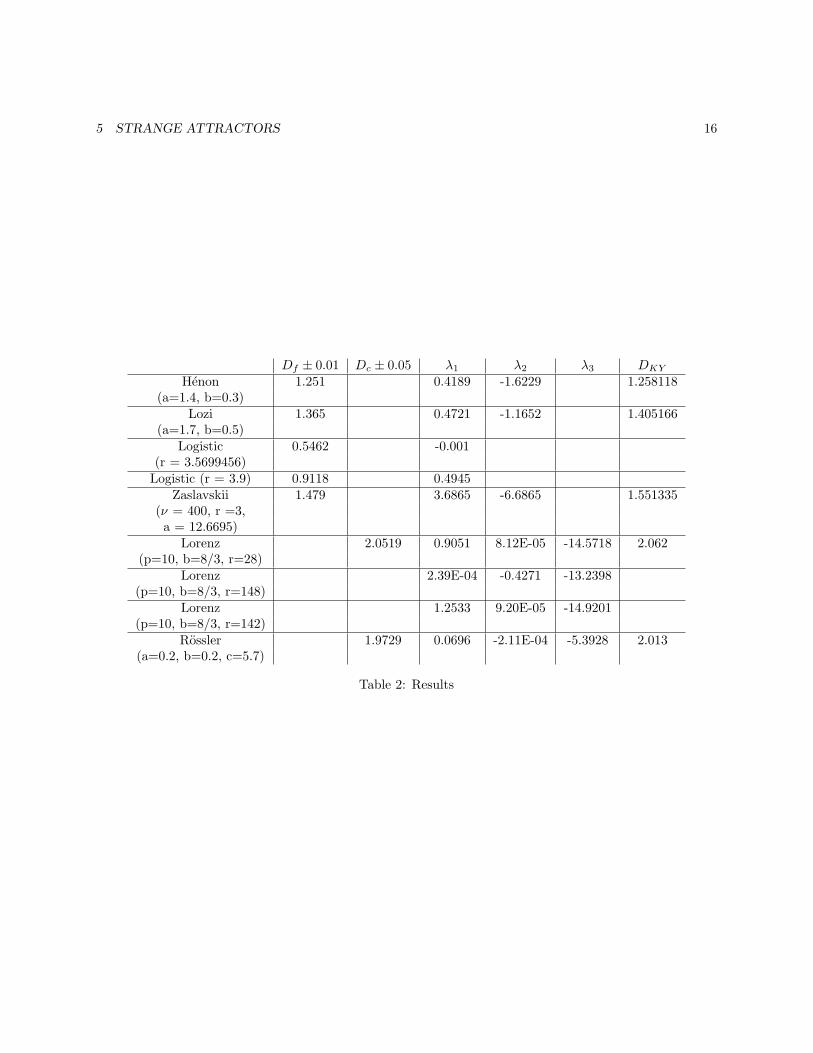
Since the amount of computer time necessary to getgood dimension estimates was enormous, I calculatedfor every strange attractor only one dimension (forevery system I also calculated the Kaplan-Yorke di-mension, which obviously wasn’t much work since I

already calculated the Lyapunov exponents of all sys-tems). For the two-dimensional maps I calculated thebox-counting dimension. For the three-dimensionalcontinuous systems I calculated the correlation di-mension.

I can immediately note that all results are indepen-dent of the initial value. For the calculation of thebox-counting dimension I checked this for 160 or 200different initial values. For the correlation dimensionI only checked five initial values, because of the com-puting time required. All the initial values gave thesame result, with, especially for the maps, very smallvariance.

For the box-counting dimension of the two-dimensional maps I would estimate the error to be±0.01 since this is how much the dimension changeswhen I change the scaling interval without getting abad fit.

For the Lorenz system and the Rossler system Iwould estimate this error to be larger. The scalinginterval I used here is very small (for the Lorenz sys-tem 0.1:0.025:0.2). This gives the best fit, but chang-ing the interval doesn’t make the fit much worse,the slope however changes significantly. So the er-ror should be at least ±0.05 and maybe even ±0.1.

All results (including the Lyapunov exponents) aregiven in table 2. In each case the Kaplan-Yorke di-mension is in good agreement with our results. Whenconsulting the literature [20, 29, 2, 3] we see that alldimensions are in rather good agreement with theliterature results.

5 STRANGE ATTRACTORS 16

Df ± 0.01 Dc ± 0.05 λ1 λ2 λ3 DKY

Henon 1.251 0.4189 -1.6229 1.258118(a=1.4, b=0.3)

Lozi 1.365 0.4721 -1.1652 1.405166(a=1.7, b=0.5)

Logistic 0.5462 -0.001(r = 3.5699456)

Logistic (r = 3.9) 0.9118 0.4945Zaslavskii 1.479 3.6865 -6.6865 1.551335

(ν = 400, r =3,a = 12.6695)

Lorenz 2.0519 0.9051 8.12E-05 -14.5718 2.062(p=10, b=8/3, r=28)

Lorenz 2.39E-04 -0.4271 -13.2398(p=10, b=8/3, r=148)

Lorenz 1.2533 9.20E-05 -14.9201(p=10, b=8/3, r=142)

Rossler 1.9729 0.0696 -2.11E-04 -5.3928 2.013(a=0.2, b=0.2, c=5.7)

Table 2: Results

REFERENCES 17

6 Conclusion

When calculating the Lyapunov exponents and di-mensions of the strange attractors of the systems Iintroduced in section 3, we see that all methods workfairly good for all systems. Only calculating the box-counting dimension of the three-dimensional systemsdidn’t work properly, but this has more to do withthe limited computer time than with a failure of thealgorithm. I also noticed clearly that doing calcula-tions with two-dimensional discrete maps was a loteasier and quicker than doing the same calculationsfor three-dimensional continuous systems, which wasto be expected.

One can find my final results in table 2. One taskfor the future could be filling in the blanks of thistable (note that some are blank because they haveno meaning for a specific system, like the second andthird Lyapunov exponent of the Logistic map). Morerecently attempts have already been made to general-ize some of these results. Investigating up to 4 ×107

low-dimensional, low order polynomial maps and or-dinary differential equations, J.C. Sprott has foundthat typically a few percent of them is chaotic [18].By investigating the strange attractors which thesechaotic maps show, he found a relation between thedimension of the phase space and the dimension ofthe strange attractor [19].

One could go further on this road and thus obtaina good estimator of the dimension of a strange at-tractor.

References

[1] Benoit B. Mandelbrot. Fractals: Form, Chanceand Dimension. W.H. Freeman and Company.

[2] David A. Russell, James D Hanson, and EdwardOtt. Dimension of strange attractors. PhysicalReview Letters, 45(14), 1980.

[3] Divakar Viswanath. The fractal property of thelorenz attractor. Physica D, 190:115–128, 2004.

[4] Edward N. Lorenz. The essence of chaos. UCLPress, 1993.

[5] Edward Ott. Chaos in dynamical systems. Cam-bridge University Press, 1993.

[6] Edward Ott, Tim Sauer, and James A. Yorke,editors. Coping With Chaos. Wiley Series inNonlinear Science. John Wiley & Sons, Inc.,1994.

[7] E.N. Lorenz. Deterministic non-periodic flow. J.Atmos. Sci., 20:130–141, 1963.

[8] Eric W. Weisstein. Henon map. FromMathworld–A Wolfram Web Resource. http://mathworld.wolfram.com/HenonMap.html.

[9] Eric W. Weisstein. Kaplan-yorke conjec-ture. From MathWorld–A Wolfram WebResource. http://mathworld.wolfram.com/Kaplan-YorkeConjecture.html.

[10] Eric W. Weisstein. Logistic map. FromMathworld–A Wolfram Web Resource. http://mathworld.wolfram.com/LogisticMap.html.

[11] Eric W. Weisstein. Lozi map. From Mathworld–A Wolfram Web Resource. http://mathworld.wolfram.com/LoziMap.html.

[12] Eric W. Weisstein. Zaslavskii map.From Mathworld–A Wolfram Web Re-source. http://mathworld.wolfram.com/ZaslavskiiMap.html.

[13] G.M. Zaslavskii. The simplest case of a strangeattractor. Physics Letters A, 69:145–147, 1978.

[14] Heinz-Otto Peitgen, Hartmut Jurgens, and Diet-mar Saupe. Chaos and Fractals: New Frontiersof Science. Springer-Verlag, 1992.

[15] Robert C. Hilborn. Chaos and Nonlinear Dy-namics. Oxford University Press, 1994.

[16] H.S. Kim, R. Eykholt, and J.D. Salas. Nonlineardynamics, delay times and embedding windows.Physica D, 127:48–60, 1999.

[17] J. C. Sprott. Simplest dissipative chaotic flow.Physics Letters A, 228:271–274.

A OSELEDEC’S MULTIPLICATIVE ERGODIC THEOREM 18

[18] J. C. Sprott. How common is chaos. PhysicsLetters A, 173:21–24, 1993.

[19] J. C. Sprott. Predicting the dimension of strangeattractors. Physics Letters A, 192:355–360,1994.

[20] J. C. Sprott. Improved correlation dimensioncalculation. International Journal of Bifurcationand Chaos, 11(7):1865–1880, 2001.

[21] J.-P. Eckmann and D. Ruelle. Ergodic theory ofchaos and strange attractors. Reviews of ModernPhysics, 57(3):617–656, 1985.

[22] J.-P. Eckmann and D. Ruelle. Fundamental lim-itations for estimating dimensions and lyapunovexponents in dynamical systems. Physica D, 56,1992.

[23] Jo Bovy and Mark Cox. Chaos en het lorenzsysteem. Theoretisch Projectwerk, Eerste licen-tie Natuurkunde, Katholieke Universiteit Leu-ven, 2004.

[24] Kaplan, J.L. and Yorke, J. A. Functional Dif-ferential Equations and Approximations of FixedPoints, page 204. Springer-Verlag, 1979.

[25] M. Henon. A two-dimensional mapping with astrange attractor. Commun. Math. Phys., 50:69–77, 1976.

[26] O.E. Rossler. An equation for continuous chaos.Physics Letters A, 57:397–398, 1976.

[27] P.-F. Verhulst. Recherches mathematiques sur laloi d’accroissement de la population. Nouv. mm.de l’Academie Royale des Sci. et Belles-Lettresde Bruxelles, 18:1–41, 1845.

[28] P.-F. Verhulst. Deuxieme memoire sur la loid’accroissement de la population. Mm. del’Academie Royale des Sci., des Lettres et desBeaux-Arts de Belgique, 20:1–32, 1847.

[29] Peter Grassberger and Itamar Procaccia. Char-acterisation of strange attractors. Physical Re-view Letters, 50:346–349, 1983.

[30] Sakire Pogun. Are attractors ’strange’, or islife more complicated than the simple laws ofphysics. BioSystems, 63:101–114, 2001.

[31] Colin Sparrow. The Lorenz Equations: Bifurca-tions, Chaos, and Strange Attractors. Springer-Verlag, 1982.

[32] Thomas Schall. Fractalkine - a strange attractorin the chemokine landscape. Immunology Today,18(4):147, 1997.

[33] V. I. Oseledec. A multiplicative ergodic theorem,ljapunov characteristic numbers for dynamicalsystems. Trudy Mosk. Obsch., 19, 1969.

A Oseledec’s multiplicative er-godic theorem

In this appendix I will state Oseledec’s multiplicativeergodic theorem [33] and it’s consequences concerningLyapunov exponents. I have taken the statement ofthis theorem from [21].

A.1 The theorem

Theorem 1 (Continuous-time Multiplicative Er-godic Theorem). Let ρ be a probability measure ona space M , and f : M → M a measure preservingmap such that ρ is ergodic. Let also T : M → them×m matrices be a measurable map such that∫

ρ(dx) log+ ‖T (x)‖ < ∞,

where log+(u)=max(0,log(u)). Define the matrixTn

x = T (fn−1x) · · ·T (fx)T (x). Then, for ρ-almostall x, the following limit exists:

limn→∞

(Tn∗x Tn

x )1/2n = Λx (50)

(We have denoted by Tn∗x the adjoint of Tn

x , andtaken the 2nth root of the positive matrix Tn∗

x Tnx )

B COMPUTER PROGRAMS 19

The logarithms of the eigenvalues of Λx are calledcharacteristic exponents. These are just the Lya-punov exponents as defined in (29). They are ρ-almost everywhere constant. So the Lyapunov ex-ponents are not dependent on the initial value, onlyin a subset of ρ-measure zero can they be different.

Let λ(1) > λ(2) > · · · be the characteristic expo-nents, no longer repeated by multiplicity; we call m(i)

the multiplicity of λ(i). Let E(i)x be the subspace of

Rm corresponding to the eigenvalues ≤ expλ(i) ofΛx. Then Rm = E

(1)x ⊃ E

(2)x ⊃ · · · and the following

holds

Theorem 2 For ρ-almost all x,

limn→∞

1n

log ‖Tnx u‖ = λ(i) (51)

if u ∈ E(i)x \E(i+1)

x . In particular, for all vectors u

that are not in the subspace E(2)x , the limit is the

largest characteristic exponent λ(1).

When we randomly choose a vector u, it willmost probably not lie in one of the special subspacesE

(i)x i > 1. So this theorem then says that we will get

the largest Lyapunov exponent when calculating thelimit. To get the ith exponent, we have to carefullyselect a vector u such that u ∈ E

(i)x \E(i+1)

x . Thismakes the computation of the other Lyapunov expo-nents very difficult.

A.2 A measure on the attractors

In order to apply these theorems to the strange at-tractors we encounter in the dynamical systems understudy in this project, we need to make sure that thereis a measure on these attractors. This measure canbe defined as follows.

We can cover the attractor with a grid of boxes(as in computing the box-counting dimension) andthen look at the frequency with which typical orbitsvisit the various boxes covering the attractor in thelimit that the orbit length goes to infinity. Whenthese frequencies are the same for all initial conditionsin the basin of attraction of the attractor except fora set of Lebesgue measure zero, then we call these

frequencies the natural measures of the boxes. Fora typical x0 in the basin of attraction, the naturalmeasure of a typical box Ci is

µi = limT→∞

η(Ci,x0, T )T

(52)

where η(Ci,x0, T ) is the amount of time the orbitoriginating from x0 spends in Ci in the time interval0 ≤ t ≤ T .

B Computer Programs

The implementation of the algorithms given in thetext were all written as m-files in Matlab. The sourcecode for all these programs can be found on my web-site http://m0219684.kuleuven.be (click on MatlabPrograms). Here you can also find some pictures ofthe strange attractors.