Luxembourg Income StudyWorking Paper No. 232

Measuring Income Inequalityin Euroland

Miriam Beblo and Thomas Knaus

Revised October 2000

1

MEASURING INCOME INEQUALITY IN EUROLAND

Miriam Beblo and Thomas Knaus*

Centre for European Economic ResearchP.O.Box 103443, 68034 Mannheim, Germany

e-mail: beblo@zew.de

Free University of BerlinBoltzmannstr. 20, 14195 Berlin, Germany

e-mail: knaus@wiwiss.fu-berlin.de

October 2000

Abstract

In this paper we propose an aggregate measure of income inequality for the founding

countries of the European monetary union. Applying the methodology of the Theil index

we are able to derive a measure for Euroland as a whole by exploiting information from

two data sets: the European Community Household Panel and the Luxembourg Income

Study. The property of additive decomposability allows us to determine each country's

contribution as well as that of each demographic group to overall income inequality. In

addition the impact of government transfers on this inequality measure is assessed.

* This study has been (co-)funded by a grant from the European Commission, TMR Programme, Access toLarge Scale Facilities and hosted by IRISS-C/I at CEPS/INSTEAD. We gratefully acknowledge commentsfrom Irwin Collier, Waltraud Schelkle and Tim Smeeding and we thank the research team atCEPS/INSTEAD for their patient support. We also thank session participants at the ESPE 2000 conferenceand at the Vereinstagung 2000 for helpful comments.

2

MEASURING INCOME INEQUALITY IN EUROLAND

Abstract

In this paper we propose an aggregate measure of income inequality for the founding

countries of the European monetary union. Applying the methodology of the Theil index

we are able to derive a measure for Euroland as a whole by exploiting information from

two data sets: the European Community Household Panel and the Luxembourg Income

Study. The property of additive decomposability allows us to determine each country's

contribution as well as that of each demographic group to overall income inequality. In

addition the impact of government transfers on this inequality measure is assessed.

3

1 Introduction

With the start of the European monetary union on the first of January 1999, all eleven

participating states now share a single currency. They have achieved an important

milestone in becoming a single economic unit which we shall refer to as Euroland 1.

However, this one event should not distract from the fact that there still remain

considerable economic, cultural as well as important social differences between the

participating nations.

With the present paper we hope to shed some additional light on this issue by estimating

an aggregate measure of income inequality within Euroland. We are interested in the

income distribution in Euroland as one indicator of the current state of a European social

union. Real income distribution comparisons are of interest to policy makers because

many people, not only as members of the current monetary but especially as potential

members of a social union, see themselves increasingly as residents of a single Euroland.

Therefore research on the current state of social cohesion within this area is needed to

provide a base point for developing and evaluating policy options down the line.

The scientific literature on this subject can be classified into three fields of research. The

first field focuses on empirical inequality measurement in general. In recent years much

progress has been made thanks to new databases such as the Luxembourg Income Study.

Examples for surveys of this literature are Atkinson, Rainwater and Smeeding (1995) and

Gottschalk and Smeeding (1997, 1998)2. The second major field is concerned with real

income comparisons 3. Work in this field includes Atkinson (1995), Gottschalk and

Smeeding (1997, 1998) and Rainwater and Smeeding (1995). Gottschalk and Smeeding

(1997, 1998) present estimates of absolute income inequality in different industrialized

1 The eleven founding members of Euroland include in alphabetical order Austria, Belgium, Finland,France, Germany, Ireland, Italy, Luxembourg, Netherlands, Portugal and Spain. Out of the 15 memberstates of the European Union (EU) only Denmark, Greece, Sweden and the UK are not part of the EuropeanMonetary Union (EMU).2 Further literature is listed on the LIS homepage at www.lissy.ceps.lu.3 Theil (1989) distinguishes two basic categories for making cross-country comparisons. Internationalincome inequality ignores the within country inequality and compares only the countries’ per capitaincome. „We obtain world inequality from international inequality by adding the average within-countryinequality“ (Theil 1989). Our approach can be assigned to the latter field of world (in our case Euroland)income inequality.

4

countries, however focussing on a different set of countries. In Rainwater and Smeeding

(1995) the real income of children in different industrialized countries is compared. The

article closest in spirit to the present paper is Atkinson (1995). He also constructs a

measure of Europe-wide income distribution but using a quite different method. Atkinson

did not employ micro-data but instead “tried the experiment of estimating the overall

distribution from national ‘meso-tables’, in that the population is divided into 40 groups

of equal size (20 groups in the case of Finland, Netherlands, Portugal and Spain), ranked

according to their equivalent disposable income, where it is assumed that incomes are

equal within each group” (Atkinson (1995), p. 13). His work also differs from ours with

respect to the definition of Europe (we do not include Norway, Sweden, Switzerland and

United Kingdom but do include Austria) and also with respect to the level of

disaggregation since we draw on the original micro-data. The third and last line of work

we refer to deals with the theory of inequality index numbers. This literature is concerned

with a specific property of inequality measures, namely additive decomposability, as

advanced by Berry, Bourguignon and Morrison (1981, 1983), Bourguignon (1979),

Cowell (1980), Shorrocks (1980), Theil (1967, 1979a, 1979b) and Yoshida (1977).

Our study adds to this earlier research by explicitly focussing on inequality in the

Euroland countries together and in the methodology to be applied. We will compare real

household equivalent incomes across countries and it is our principal objective to

aggregate the inequality measures into a single inequality measure for Euroland as a

whole. We believe that such measures will be an essential part of future discussion about

a European social union. The major difference of our study is the special focus we

employ on a hypothetical Euroland around the mid-1990s. Using data from Wave 2

(1995) of the European Community Household Panel (ECHP) together with data from the

Luxembourg income study (LIS) in the mid 1990s, inequality in every single country will

be measured as will be overall inequality of household equivalent income in Euroland. Of

course at that point in history one could only speak of the group of countries that would

ultimately form a future Euroland. Documenting the heterogeneity of the social structures

of the individual states at a time when a prospective monetary union just came into view

is nevertheless most interesting, especially with regard to the current discussion about

potential future entry of the non-participating countries (the remaining EU countries

5

Denmark, Greece, Sweden and the United Kingdom as well as Eastern European

countries joining the EU). We believe that our attempt to aggregate national inequality

measures for Euroland constitutes a genuine contribution since it exploits methodology

used to analyze inequality in regions of flexible size like Euroland that will admit new

members in the foreseeable future. To our knowledge this could very well be the first

approach to quantify aggregate inequality in Euroland at a time when information about

social structures in Euroland is still rather limited.

We use a summary measure of the generalized entropy family of inequality indices, the

Theil inequality index, due to its distinct advantage of being an additively decomposable

measure. This property allows us to derive an inequality index for Euroland as a whole, in

spite of the fact that complete information on all participating countries in the data sets is

not available. Applying the methodology of the Theil index we are still able to compute a

measure for Euroland income inequality when we combine data of the ECHP, that do not

include Finland, with LIS-data that do not include Portugal.

Additive decomposability further allows us to determine each country's and household's

contribution to overall income inequality in Euroland. By using an additively

decomposable measure, we can compare the country effect and the household structure

effect within each country with the Euroland average and assess the relative contribution

of both effects.

Finally we analyze the redistributive impact of transfer policies in the different Euroland

countries for different inequality measures upon (aggregate) Euroland inequality. By

comparing the distributions of net total incomes (including governmental and social

insurance transfers) with pre-transfer (but post-tax) incomes are able to estimate the

effectiveness of government transfers in the Euro countries.

The paper proceeds as follows: we begin with a discussion of real income comparisons

across countries along with an introduction to the data sets used. Next the methodology of

measuring income inequality with an additively decomposable measure is described. We

then present the results for overall inequality in Euroland and a decomposition of this

index with respect to the Euro countries. This is followed by a decomposition by

countries as well as demographic groups to investigate their respective contributions to

6

measured inequality in Euroland. In addition the effect of social transfer payments on the

distribution of income will be analyzed. The paper concludes with a summary of the main

findings.

2 Concepts and Data

Since a comparison of income distributions across countries raises a host of problems and

important issues, we want to be sure that we know what it is precisely that we want to

measure. Second, choices must be made to achieve comparability among people living in

households of different sizes and in different countries.

Our analysis limited to the distribution of disposable money income. That is, rather than

basing measured inequality on consumption or expenditure data, we take total annual

household income after taxes and transfer payments as our chosen indicator for

differences in the access to economic resources or achievable economic well-being. Since

we are particularly interested in comparing real income levels across all countries that

constitute Euroland we first have to transform all incomes into comparable monetary

values in an appropriate manner. All income amounts have been reported in national

currency units and are converted to a comparable base using the multilateral purchasing

power parities provided by Eurostat for the reference year.4

We measure income as household equivalent income, i.e. adjusted for family size. The

unit of analysis is the individual to whom we assign an equivalent household income

according to the modified OECD scale 5. Insofar as household structures differ across

countries, the choice of the equivalence scale may indeed affect the result of the income

comparison. This problem is taken care of by sensitivity analyses using different scales.

We multiply the household equivalent income by the number of individuals in each

household, thereby assuming that within each family an equal share of income is

allocated to each member. Thus we do not take into account the possibility of unequal

4 In sensitivity analyses different conversion rates have been used to transform national currencies intoECU (in particular ECU exchange rates from 1994 and EURO exchange rates from 1999), but these turnout not to have a substantial effect on the final measure.5 With the modified OECD scale a weight of 1 is assigned to every household member above the age of 16.Every additional adult (person over 16) receives the weight 0.5 and each child under 16 receives the weight0.3.

7

sharing within the household. While clearly a very strict assumption, this is standard

assumption in income distribution research typically little or no information is available

about income distribution within families.6

Since time spent in gainful employment is in most cases not the sole productive activity

of a household, it would be necessary to also account for the yields of household

production, as for instance the value of a cooked meal or a well-educated child and not

just market income. However in the present study household production is ignored due to

data constraints. For this reason the results need to be interpreted cautiously as inequality

might be overestimated when there are households in which home-produced goods make

up a major share of a family’s total real consumption. In a comparison of inequality

measures across countries the respective relevance of household production should be

kept in mind when interpreting differing indices.

A very rich and only recently issued data set to investigate the distribution of income

across European countries is provided by the European Community Household Panel

(ECHP). To meet the demand for greater in-depth knowledge and better compatibility of

data on social and economic conditions in the European Union, the ECHP was launched

as a closely coordinated component of a system of household surveys aimed at generating

comparable social statistics at the EU level. The ECHP is a standardized survey

conducted in Member States of the European Union under the auspices of the Statistical

Office of the European Communities7. It involves annual interviewing of a representative

panel of households and individuals in each country, covering a wide range of topics on

living conditions. The ECHP includes comparable information across Member States

regarding income, work and employment, poverty and exclusion, housing, health and

many other social indicators. The key feature of the ECHP is harmonization of its

methodology, specifically through the creation of a centralized questionnaire that serves

as the point of departure for all national surveys. Although this common questionnaire

6 It should be noted that by focussing on disposable money income we ignore two factors that also affectfamily well-being and may vary widely across countries (Gottschalk and Smeeding 1998). The first is anysort of in-kind income including private and publicly provided goods. The second concerns indirecttaxation.7 For a detailed description of the ECHP methodology and questionnaires see Eurostat 1996, The EuropeanCommunity Household Panel (ECHP): Volume 1- Survey methodology and Implementation and The

8

ensures a common conceptual framework and comparability of the national surveys, it

does not necessarily imply the use of identical questions among countries. On the

contrary, because of differing legal and institutional frameworks, the same information,

e.g. on income and social transfers, is sometimes provided by very different questions

(Eurostat 1998).

To assess the quality of the ECHP, data comparisons with other EU and national sources

have been made (Eurostat 1998). Income distribution in the ECHP, the most important

feature for our analysis, has been compared with the national consumption and

expenditure surveys showing that the overall mean income level is higher in the ECHP.

But the differences are only marginal and they are most pronounced in those countries

where the consumption-expenditure survey is known to be of limited quality with respect

to income data (Eurostat 1998).

To study income inequality in Euroland we need income data on all eleven founding

members of the European monetary union. Since to date only waves 1 and 2 of the

ECHP, gathered in 1994 and 1995, are available, information for Finland is lacking,

because it first joined the ECHP in 1996. For this reason we draw on data from the

Luxembourg Income Study (LIS)8. The LIS is a collection of micro data sets obtained

from a range of income surveys in various countries. Information on income and

household characteristics has been made comparable to improve consistency across

countries. Thus the major difference between the ECHP and the LIS is that while the LIS

data provide information that has been drawn from national surveys and made

comparable ex post, the ECHP has been started with a common conceptual framework

and standardized content from the very beginning.

With both data sets, the 1995-wave of the ECHP for ten of the Euro countries and the

1995-LIS file on Finland, we have assembled all the ingredients required to estimate an

inequality measure for Euroland as a whole.

European Community Household Panel (ECHP): Volume1 – Survey questionnaires: Wave 1-3 – Theme 3,Series E, Eurostat, OPOCE, Luxembourg, 1996.8 Further information at www.lissy.ceps.lu. See particularly de Tombeur and O’Connor (1995).

9

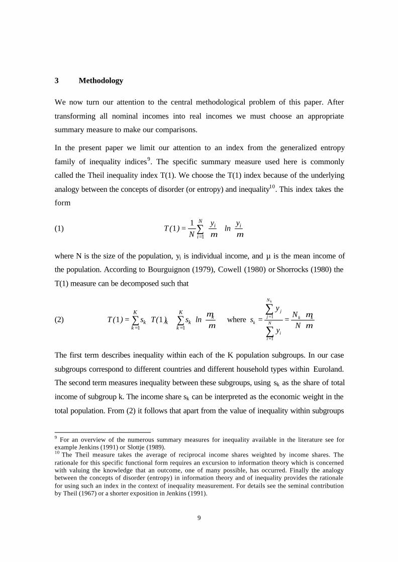
3 Methodology

We now turn our attention to the central methodological problem of this paper. After

transforming all nominal incomes into real incomes we must choose an appropriate

summary measure to make our comparisons.

In the present paper we limit our attention to an index from the generalized entropy

family of inequality indices9. The specific summary measure used here is commonly

called the Theil inequality index T(1). We choose the T(1) index because of the underlying

analogy between the concepts of disorder (or entropy) and inequality10. This index takes the

form

(1) ∑=

⋅

=

N

i

ii yln

yN

)(T1

11

µµ

where N is the size of the population, yi is individual income, and µ is the mean income of

the population. According to Bourguignon (1979), Cowell (1980) or Shorrocks (1980) the

T(1) measure can be decomposed such that

(2)

⋅+⋅= ∑∑

== µµk

K

kk

K

kkk lns)(Ts)(T

1111 where

µµ

⋅⋅==

∑

∑

=

=

NN

y

ys kk

N

ii

N

jj

k

k

1

1

The first term describes inequality within each of the K population subgroups. In our case

subgroups correspond to different countries and different household types within Euroland.

The second term measures inequality between these subgroups, using sk as the share of total

income of subgroup k. The income share sk can be interpreted as the economic weight in the

total population. From (2) it follows that apart from the value of inequality within subgroups

9 For an overview of the numerous summary measures for inequality available in the literature see forexample Jenkins (1991) or Slottje (1989).10 The Theil measure takes the average of reciprocal income shares weighted by income shares. Therationale for this specific functional form requires an excursion to information theory which is concernedwith valuing the knowledge that an outcome, one of many possible, has occurred. Finally the analogybetween the concepts of disorder (entropy) in information theory and of inequality provides the rationalefor using such an index in the context of inequality measurement. For details see the seminal contributionby Theil (1967) or a shorter exposition in Jenkins (1991).

10

T(1)k, inequality depends on mean income levels µk and population sizes Nk. Hence, once

we have the countries' inequality indices, all we need to determine overall inequality are

these aggregate macroeconomic numbers.

The generalized entropy family in general and the Theil index T(1) in particular satisfy the

axioms of symmetry (anonymity), population replication (population homogeneity,

replication invariance), mean independence (invariance to relative changes, scale invariance,

homogeneity), the Dalton-Pigou principle of transfers (strong principle of transfers) and

additive decomposability. The last property implies that an overall inequality measure can

be additively decomposed into its subgroups' distinct inequality measures as has been shown

in (2) above11.

Additive decomposability is the condition we impose when choosing our inequality

measure12. Of course, there are objections in that it requires a certain degree of

independence between subgroups. It is not entirely intuitive why inequality in one group

should be independent of inequality in another group. But in this particular case the different

groups represent different countries. Here it seems sensible to allow inequality in Germany

to be independent of inequality, say, in Portugal. Whether the assumption of independence

still holds with the introduction of a common currency and monetary policy in 1999 is a

subject for further discussion. In the words of Cowell (1998), the property displayed in (2)

suggests a “natural cardinalization” of decomposable measures. In our context, it is an

appropriate decomposition for revealing the pattern of inequality in Euroland.

Instead of calculating the T(1) index an alternative choice would be the T(0) index –also

called the mean logarithmic deviation which has the property of being even more bottom

sensitive than the T(1). We choose the T(1) index because our main purpose is to draw a

11 Two remarks about other often used axioms are in order here. First, T(1) is not normalized between 0 and 1so it does not satisfy the axiom of normalization. Dividing T(1) by ln(N) achieves normalization. Second, T(1)is bottom-sensitive because observations are weighted by the size of their incomes, i.e. the axiom of transfersensitivity is satisfied at the bottom end of the distribution. A 100 ECU transfer from someone with 100,000ECU to someone with 90,000 ECU would alter T(1) by as much as one from someone with 10,000 ECU tosomeone with 9,000 ECU. The change in T(1) depends on the relative incomes of the households involved inthe transfer. Whether this implicit form of sensitivity to transfers in the T(1) measure is the appropriate oneremains of course subject to discussion.12 The priority of additive decomposability is the reason for using the non-normalized T(1) measure, i.e. inour case maximum possible inequality in a group depends on population size. The intuition behind this isthat a society with a million people where one person receives all income is more unequal than a societywith one thousand inhabitants where one person receives the total income.

11

picture of the income distribution in Euroland and not evaluate the effectiveness of

distribution policies. The crucial advantage of the T(1) measure for the analysis presented

here lies in its use of economic weights or income shares instead of using sole population

shares (as in the T(0) measure). While population shares are part of income shares as can be

seen from (2) the latter also include relative mean incomes. We consider economic weights

or income shares more appropriate since they better reflect countries' economic standings in

terms of political power within the EMU than pure population sizes.

Indices other than those belonging to the Theil family do not satisfy what Cowell (1998)

labels the “accountant’s approach” to decomposition, meaning that the weighted within-

group inequality terms together with the between-group inequality term sum to unity a very

useful property in our context. This accounting property illustrates that the overall inequality

is not just the simple sum of individual inequalities in which case it would be sufficient to

look at the differences of individual inequality measures to evaluate the degrees of

heterogeneity between countries. However, when viewing all countries together as a single

entity, overall inequality is the sum of weighted inequality indices and appropriately

measured between-group inequality. In view of the economic and social process of

integration that is reflected in a single European market and a single European Currency

area we think it worthwhile to consider inequality within Euroland as a whole. For this

reason we look at real rather than nominal inequality as usually done in the scientific

literature.

One major reason why we actually need additive decomposability to be satisfied is that

Euroland consists of eleven countries. In the 1995-wave of the ECHP, however, Finland

was not yet included in the data set. As a consequence we first have to calculate a proxy

measure for overall Euroland inequality including only ten countries, i.e. with Finland

missing. The value of this "Euro10"-Theil index then has to be adjusted by Finland's

contribution to total inequality by exploiting additional information provided by the LIS.

It is at this point where the properties of the Theil index T(1) come into play: the Theil

index can be calculated with aggregate data, in particular the population share, the mean

income and the Theil (inequality) index of every population subgroup as shown in (1) and

(2). Hence, if we dispose of T(1) indices of all participating nations as well as their

12

respective population shares and mean incomes, we can simply "sum" everything

according to equation (2).

Looking closer at the changes that result when integrating a new country into an existing

entity, we can discriminate four effects:

(3)

( )[ ]4444444 34444444 214444 34444 21

44 344 2144 344 21

?IV

K

kKkK

k

K

kK

kKk

III

K

kk

Kk

Kk

?II

KKK

K

I

KKK

KK

lnslns)(Tss

lns)(Ts)(T)(T

0

111

1

0

1

1

0

111

1

0

111

1

1

111

<>

==+

+

≤

=

+

<>

+++

+

≥

+++

+

⋅−

⋅+⋅−+

⋅+⋅=−

∑∑∑µµ

µµ

µµ

where subscript k represents subgroup k as before and superscript K represents the total

number of all K subgroups.

One direct (positive) effect from adding another country with inequality T(1)K+1 is quite

obvious when inspecting (2). Technically speaking we are now summing over (K+1)

groups instead of K groups. As long as the added country has at least some degree of

inequality, i.e. (T(1)K+1 >0), aggregate inequality will always be greater in the new bigger

entity. This direct inequality effect is captured by the first term in equation (3) above. The

sign of term II depends on the relative size of the new country's mean income level µK+1

with respect to that of the existing entity (µK+1≠µK). If the entrant's mean income is larger,

there will be a positive mean income effect, otherwise we will observe a negative impact

on aggregate inequality.

Effect III and IV are both re-weighting effects. The third term is unambiguously negative.

When adding another country, overall population and overall mean income will be

altered. This again will affect the weights assigned to the existing (old) countries. Since

every country k is weighted by its economic share sk, its contribution to overall inequality

will always be smaller in the new bigger entity. As a result the re-weighting inequality

effect III and the direct inequality effect I work in opposite directions. The sign of the last

term IV is ambiguous again. It depends on the relation between the new overall mean

income and the old overall mean income which we can call the re-weighting mean

income effect. If the entrant's income level leads to a rise in overall mean income, the re-

13

weighting mean income effect will be negative. It will be positive if a relatively poor

country enters. As a result, the sign of the combined effect of the four partial effects

remains also unclear, i.e. it is not determined ex-ante.

In our example of Euroland we can now assess empirically what the net effect will be

when adding the data from Finland to the inequality measure based on the ECHP data set.

Calculating the Euro10-Theil according to equation (2) generates an inequality index of

0.1849. Integrating Finland's income and population data with reference to equation (3)

then yields an overall Euro-Theil of 0.1831.13 On the right hand side of equation (4) we

can discriminate the following four effects:

(4) 0.1831 - 0.1849 = 0.0018 + 0.0016 - 0.0033 - 0.0018.

The resulting net effect of including Finland is thus -0.0018, i.e. there is less than one

percent difference between the two indices14. The direct inequality effect (first term), the

between-group or mean income effect (second term) and the re-weighting inequality

effect (third term) more or less level each other out. So the major part of the overall

change can be attributed to between-group re-weighting caused by a higher overall mean

income after integrating Finland into our empirical Euroland (fourth term).

This analysis gives us an impression of the mechanics behind the Theil T(1) inequality

measure that relies on differences not only in incomes but also in population sizes. The

property of additive decomposability has been exploited to construct a measure for

inequality in Euroland as a whole. We find this measure not to differ very much from the

Euro10-Theil calculated for only those ten countries included in the ECHP. This finding

allows us to focus our further analyses on those ten countries using the Euro10 results as

a proxy for the structure of the income distribution within all of Euroland.

13 For a comparison, note that the US-Theil index calculated using LIS-data from 1994 amounts to 0.2289.14 We use a one percent rule of thumb as a rough substitute for more rigorous statistical inference that mustawait future work. The small differences in the T(1) measures may not come as a surprise since Finland is avery small country with a population share of less than two percent of the Euroland population. The sameholds true for the income share. Furthermore Finland is consistently found to be one of the less unequalcountries in international comparisons as for example in Atkinson, Rainwater and Smeeding (1995).

14

4 The structure of income inequality in Euroland

Having constructed and evaluated a measure of overall inequality in Euroland we are now

interested in determining the various sources of this income inequality. How much does

each nation contribute to the overall inequality index of 0.18 and which share of the

income distribution can be traced back to demographic groups? First we will present the

decomposition of the inequality measure by countries. Then we turn to the decomposition

by countries and household types to answer the question which of these characteristics is

the driving force for the observed income inequality in Euroland.

4.1 Decomposition by countries

Let us start with a closer inspection of the nations' population shares within the Euroland

income distribution. At first glance, the most striking feature are the great discrepancies

in population sizes across Euro countries as can be seen in Table 1.

We have Germany, France and Italy with an average population share of 20 percent and

more on the one hand. On the other hand, there are six very small countries that constitute

only 5 percent and less (Luxembourg with a share of a sixth of a percentage point) of the

Euroland population. Spain is in the middle ranks with 14 percent of all residents.

Population shares within the income deciles differ very much from these average country

means. However, there is no clear relationship between income distribution and absolute

country size. Instead, as one might expect, geography matters a lot. Whereas the central

or continental Euro countries are over-proportionally represented in the higher income

deciles, the Southern-European states Italy, Spain and Portugal (as well as Ireland in the

North) have larger shares in the lower income groups. For instance about 20 percent of all

households in the bottom decile and 42 percent of the top income decile of Euroland are

from Germany, that has an overall population share of 29 percent. The Portuguese on the

contrary, having a mean population share of 3.5 percent, constitute almost 11 percent of

the poorest and hardly more than 1 percent of the highest earners in Euroland.

The overall pattern of over- and under-representation of nationalities within the deciles

becomes even more visible by examining the standardized share of each country

according to its actual population size, the representation rate, over the Euroland income

15

distribution. In Figures 1A and 2A (in the Appendix) the decile population shares are

standardized by each country's overall population share. A representation rate above 1

indicates that the country is responsible for more people in that income group than its

average population size would predict, hence this nation is over-represented in the

respective income class.

Table 1: Income distribution in Euroland (Deciles)

IncomeG NL BE LU F IRL I S P A EURO

LAND

decilePopulation share in %

1 20.1 3.2 2.4 0.04 8.6 1.2 26.2 26.0 10.6 1.7 100

2 13.2 2.2 2.3 0.02 14.6 2.6 31.7 25.4 6.6 1.6 100

3 20.7 5.1 2. 5 0.02 18.2 1.6 25.6 19.4 5.0 2.0 100

4 21.8 7.5 3.3 0.04 20.8 1.1 24.4 15.2 3.6 2.5 100

5 27.9 7.4 3.3 0.05 23.0 1.1 19.4 13.0 2.5 2.4 100

6 33.6 6.4 3.5 0.09 21.8 0.9 18.7 10.3 1.7 3.1 100

7 33.8 6.1 4.3 0.10 22.2 1.1 18.2 9.3 1.4 3.7 100

8 37.5 6.0 4.7 0.20 22.9 0.9 15.2 7.9 1.4 3.4 100

9 38.0 5.7 5.4 0.25 25.5 1.2 12.8 6.0 1.2 4.1 100

10 42.0 4.9 4.7 0.60 26.2 1.2 9.3 6.2 1.4 3.7 100

Mean 28.9 5.4 3.6 0.14 20.4 1.3 20.1 13.9 3.5 2.8 100

Source: Authors‘ calculations, ECHP (wave 1995)

In Figure 1A the graphs of the group of central Euro countries Germany, France,

Belgium, Austria and Luxembourg are clearly upward-sloping with increasing income

decile. They switch from under-representation to over-representation somewhere between

the fourth and the sixth decile. Luxembourg is an extreme case with a population share

lower than half its mean population share in the lower half of the income distribution and

a substantial over-proportional fraction in the highest decile. An exception to this central

European pattern are the Netherlands that, after a remarkable over-representation in the

fourth and fifth decile, experience a decrease of their population share in higher income

classes.

16

Italy, Spain and Portugal also reveal a common downward-sloping pattern as illustrated

in Figure 2A: Whereas the lowest 30 to 40 percent of incomes are relatively often

received by Southern European residents, higher incomes are under-represented in these

countries. Among the poorer states of Euroland, Ireland stands out of line due to its

relatively high level of social security protection in the bottom deciles. With a most

pronounced over-representation in the second decile and a sharp drop thereafter the Irish

even improve their representation rate throughout the 40 percent highest income earners

from 0.7 to almost 1. In other words the share of Irish among Euroland's highest income

earners is almost equivalent to their average population share.

With this indirect information about the national structures of the income distribution we

now turn to the entropy measure and its more immediate since compressed indication of

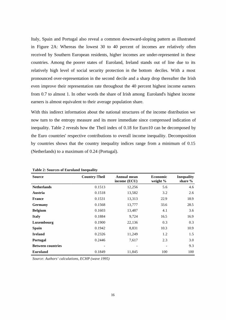
inequality. Table 2 reveals how the Theil index of 0.18 for Euro10 can be decomposed by

the Euro countries' respective contributions to overall income inequality. Decomposition

by countries shows that the country inequality indices range from a minimum of 0.15

(Netherlands) to a maximum of 0.24 (Portugal).

Table 2: Sources of Euroland Inequality

Source Country-Theil Annual meanincome (ECU)

Economicweight %

Inequalityshare %

Netherlands 0.1513 12,256 5.6 4.6

Austria 0.1518 13,582 3.2 2.6

France 0.1531 13,313 22.9 18.9

Germany 0.1568 13,777 33.6 28.5

Belgium 0.1603 13,487 4.1 3.6

Italy 0.1884 9,724 16.5 16.9

Luxembourg 0.1900 22,136 0.3 0.3

Spain 0.1942 8,831 10.3 10.9

Ireland 0.2326 11,249 1.2 1.5

Portugal 0.2446 7,617 2.3 3.0

Between countries - - - 9.3

Euroland 0.1849 11,845 100 100

Source: Authors‘ calculations, ECHP (wave 1995)

17

We can broadly distinguish three groups of states. Income is most equally distributed in

the central or continental Northern European countries (Austria, France, Germany,

Netherlands) where the Theil index takes a value of about 0.155 with a variation below 1

percent across countries. Also worth noting is that these countries have mean incomes

that are remarkably equal (12,000 to 14,000 ECU). Next comes the Southern European

group consisting of Italy and Spain plus Luxembourg as a geographical outlier. The

inequality measures in this second group vary only a little around 0.19 whereas average

income levels deviate drastically. The "periphery" consisting of Ireland and Portugal

show greatest income inequality at about 0.24.

In terms of relative contributions we can see that the four largest countries Germany,

France, Italy and Spain make up 75 percent of the overall Theil index. Differences

between countries also account for almost 10 percent of Euroland inequality. This leaves

only 15 percent to the remaining six countries. Interestingly, the actual income inequality

does not show great variation across countries. It is instead the economic weights of the

states that differ remarkably. The differences in economic weights are due to the

countries' mean income levels as well as their population sizes. By construction of the

Theil measure these weights play an important role in assessing an aggregate index for

Euroland. As a result Germany comes in first in terms of relative contributions although

its index is the fourth lowest of all country-Theils. Germany is responsible for a share of

28.5 percent of overall inequality, since it constitutes almost 30 percent of the Euroland

population. In contrast to this, Luxembourg brings up the rear by contributing only 0.3

percent of the aggregate measure despite its relatively high within-country income

inequality. This is due to its average population share under 0.14 percent of all Euroland

residents.

As noted earlier, the neglect of production within the household might lead to a bias in

the inequality measures presented, since our comparisons are based on earned market

income alone. If household production plays a greater role in Southern Europe and

Ireland inequality will actually be smaller and the difference to Central Europe will also

be smaller than the numbers suggest. This overestimation is confirmed by a sensitivity

analysis with different household equivalence scales. As soon as a higher weight is

18

assigned to children, an indication for household production taking place, the indices

have slightly lower values. This especially applies to Ireland and Portugal.

4.2 Decomposition by countries and by demographic groups

After having accounted for the sources of Euroland inequality with respect to countries,

we now focus on a further decomposition of inequality by demographic groups/household

structures.

Table 3: Theil T(1) indices by country and household type

Age head of the household

≥≥60 <60 with children <60; no children All hh

Netherlands 0.1566 0.1074 0.1693 0.1513

Austria 0.1114 0.1389 0.1661 0.1518

France 0.1890 0.1346 0.1461 0.1531

Germany 0.1566 0.1528 0.1501 0.1568

Belgium 0.2009 0.1277 0.1636 0.1603

Italy 0.1968 0.1855 0.1742 0.1884

Luxembourg 0.2606 0.1483 0.1807 0.1900

Spain 0.1674 0.2179 0.1763 0.1942

Ireland 0.2884 0.1769 0.2380 0.2326

Portugal 0.2651 0.2405 0.2174 0.2446

Euroland 0.1962 0.1743 0.1772 0.1849

Source: Authors‘ calculations, ECHP (wave 1995)

We divide the population into households in which the head of the household is older

than 60 years and in those with younger heads. We also partition the younger households

into those with and those without children. With this admittedly very rough

categorization of households, we hope to capture the principle forces at work with respect

to aggregate Euroland inequality. We would like to determine whether household types or

country differences are primarily responsible for the observed structure of the income

distribution in the European Monetary Union.

The purpose of this disaggregation is twofold. First we want to compare measured

inequality across all subgroups. Second we want to evaluate the contribution of each

19

group to overall inequality. An additional question would be whether differences between

particular inequality measures can be explained by different structures of social security

expenditures in the ten member states.

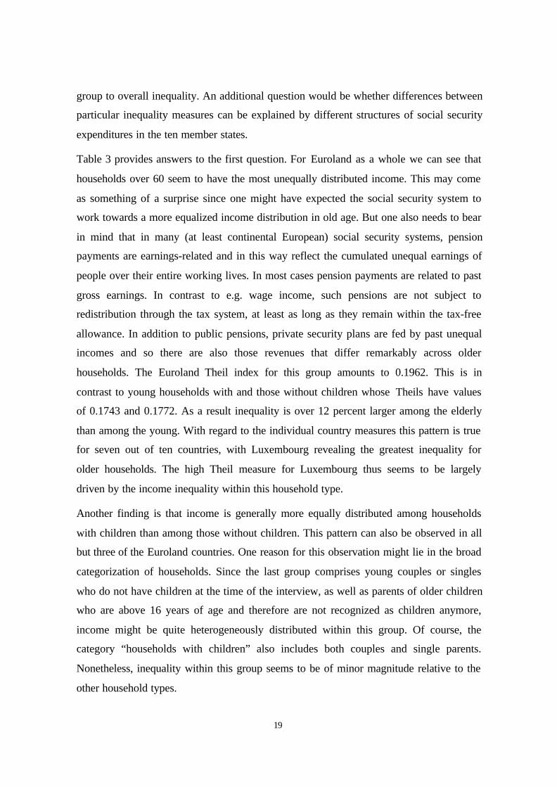
Table 3 provides answers to the first question. For Euroland as a whole we can see that

households over 60 seem to have the most unequally distributed income. This may come

as something of a surprise since one might have expected the social security system to

work towards a more equalized income distribution in old age. But one also needs to bear

in mind that in many (at least continental European) social security systems, pension

payments are earnings-related and in this way reflect the cumulated unequal earnings of

people over their entire working lives. In most cases pension payments are related to past

gross earnings. In contrast to e.g. wage income, such pensions are not subject to

redistribution through the tax system, at least as long as they remain within the tax-free

allowance. In addition to public pensions, private security plans are fed by past unequal

incomes and so there are also those revenues that differ remarkably across older

households. The Euroland Theil index for this group amounts to 0.1962. This is in

contrast to young households with and those without children whose Theils have values

of 0.1743 and 0.1772. As a result inequality is over 12 percent larger among the elderly

than among the young. With regard to the individual country measures this pattern is true

for seven out of ten countries, with Luxembourg revealing the greatest inequality for

older households. The high Theil measure for Luxembourg thus seems to be largely

driven by the income inequality within this household type.

Another finding is that income is generally more equally distributed among households

with children than among those without children. This pattern can also be observed in all

but three of the Euroland countries. One reason for this observation might lie in the broad

categorization of households. Since the last group comprises young couples or singles

who do not have children at the time of the interview, as well as parents of older children

who are above 16 years of age and therefore are not recognized as children anymore,

income might be quite heterogeneously distributed within this group. Of course, the

category “households with children” also includes both couples and single parents.

Nonetheless, inequality within this group seems to be of minor magnitude relative to the

other household types.

20

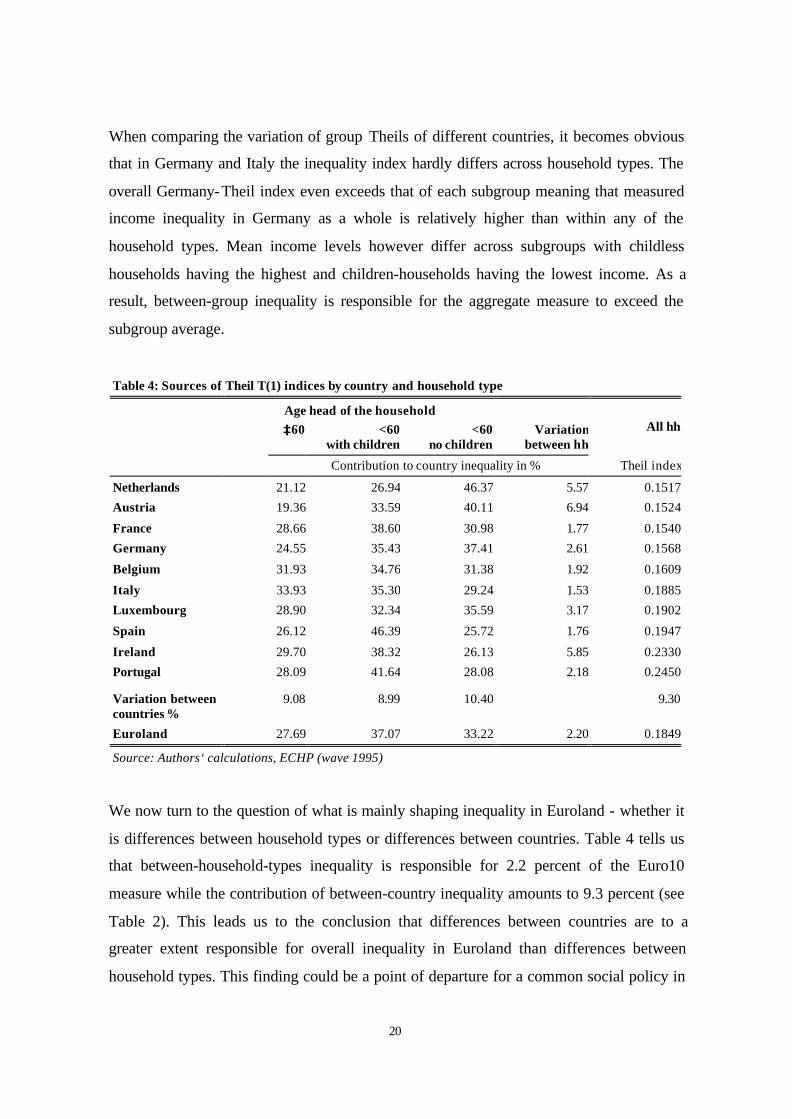
When comparing the variation of group Theils of different countries, it becomes obvious

that in Germany and Italy the inequality index hardly differs across household types. The

overall Germany-Theil index even exceeds that of each subgroup meaning that measured

income inequality in Germany as a whole is relatively higher than within any of the

household types. Mean income levels however differ across subgroups with childless

households having the highest and children-households having the lowest income. As a

result, between-group inequality is responsible for the aggregate measure to exceed the

subgroup average.

Table 4: Sources of Theil T(1) indices by country and household type

Age head of the household

≥≥60 <60 with children

<60no children

Variationbetween hh

All hh

Contribution to country inequality in % Theil index

Netherlands 21.12 26.94 46.37 5.57 0.1517

Austria 19.36 33.59 40.11 6.94 0.1524

France 28.66 38.60 30.98 1.77 0.1540

Germany 24.55 35.43 37.41 2.61 0.1568

Belgium 31.93 34.76 31.38 1.92 0.1609

Italy 33.93 35.30 29.24 1.53 0.1885

Luxembourg 28.90 32.34 35.59 3.17 0.1902

Spain 26.12 46.39 25.72 1.76 0.1947

Ireland 29.70 38.32 26.13 5.85 0.2330

Portugal 28.09 41.64 28.08 2.18 0.2450

Variation betweencountries %

9.08 8.99 10.40 9.30

Euroland 27.69 37.07 33.22 2.20 0.1849

Source: Authors‘ calculations, ECHP (wave 1995)

We now turn to the question of what is mainly shaping inequality in Euroland - whether it

is differences between household types or differences between countries. Table 4 tells us

that between-household-types inequality is responsible for 2.2 percent of the Euro10

measure while the contribution of between-country inequality amounts to 9.3 percent (see

Table 2). This leads us to the conclusion that differences between countries are to a

greater extent responsible for overall inequality in Euroland than differences between

household types. This finding could be a point of departure for a common social policy in

21

Euroland. Such a policy, rather than reducing the differences between demographic

groups within countries, should be aimed at reducing income inequality between

household types across countries.

This conclusion is supported by the observation that there is large cross-country variation

of inequality indices within household types. Going back to Table 3, we see that

inequality for households over 60 varies between 0.11 in Austria and almost 0.29 in

Ireland. This span is significantly larger than the overall span (0.15 to 0.24) found in (4.1)

above. At the same time the between-group variation among these households is below

the overall between-country variation. This indicates that although inequality within this

demographic group varies a lot across countries, mean income differences seem to be of

minor magnitude.

The same holds true, though to a lower extent, for the Theil measure for households with

children. Here the T(1) index ranges between 0.11 in the Netherlands to 0.24 in Portugal.

That is, in the Netherlands households with children have a Theil index 60 percent below

the aggregate measure of 0.18 whereas Portuguese families face an income inequality

exceeding the Euroland average by 30 percent. Again the mean income deviation

between countries accounts for 9 percent of overall inequality in this group.

Only for the last household type (household head under 60, no children) is the range of

country measures the same as for all household types together, although the relative

rankings of the countries differ. Most importantly, between country variation contributes

10.4 percent of the Euroland measure meaning that although the country indices do not

differ much, mean incomes do. Thus, convergence in social security among EMU

members might reduce inequality between countries disproportionately.

To develop some intuition for the differing indices, a look at European social security

payments is quite revealing (Europäische Kommission 1999). That elderly people in

Ireland experience the greatest income inequality, deviating from the overall Euroland

index by almost 56 percent, corresponds to its lowest share of social expenditures for

elderly people and surviving dependents in comparison to other EU countries. High

income inequality for Portuguese and Spanish households with children is consistent with

having the lowest per-capita payments to families and children, in particular lowest levels

22

of child benefit payments, among the member states of the European union. In Spain the

share of social expenditures for families relative to GDP compared to the same figure for

the elderly reveals a ratio of 1:24. In comparison the ratio for Germany is 1:5 and for

Ireland it is 1:2.

The relationship between a country’s social security budget relative to GDP and its Theil

measure for the year 1994 can be seen in Figure 3A as a definitely pronounced negative

relationship. The higher social security payments in terms of GDP the lower is income

inequality. While this comparison does not tell us anything about the efficiency of social

security systems, it provides information on the degree of similarity among the Euroland

countries with respect to income inequality as well as to the role of the state.

Interestingly, the clustering of countries into three groups already noted with respect to

the inequality indices is also seen in the share of social security expenditures.

However, in order to gauge the impact of social transfer payments on the income

distribution within countries, it is useful to compare pre-transfer and post-transfer

incomes.

5 The redistributive impact of social transfers in Euroland

A comparison of the distribution of net total incomes (including social transfers)

standardized by a household equivalence scale with that of pre-government (but post-tax)

incomes indeed yields another striking result shown in Table 5. Prior to social transfer

payments hardly any differences in the (very high) Theil measures exist between

countries. Government intervention not only reduces inequality but also appears to

intensify differences between countries. The variation of country Theils even increases

after social transfer payments. It seems that more wealthy states (like the Benelux,

Germany or France) can afford to shift the incomes of their poor to a greater extent than

less wealthy states (like Ireland and Portugal) can; thereby enhancing the disparities in

country mean incomes. The relative contribution of between-country differences in

overall inequality rises substantially from 3.4 percent before transfers to 9.3 percent after

social transfer payments.

23

While prior to transfers the relation between countries' mean incomes and their Theil

measures reveal little relationship to each other adding social protection we find the

correlation substantially more negative. We saw this relationship in the previous section

in Figure 3A in the Appendix. This supports the conjecture from earlier that richer

countries have more extensive social protection schemes in order to lower the gap

between high and low income earners. Of course this says nothing about the causality of

this relationship.

It is also interesting to note that there is a very high negative relationship between the

relative size of the redistribution (as measured by the ratio of post-government to pre-

government Theil) and the degree of social protection expenditures.15 There is also no

clear relationship between pre-government mean income and the pre-government T(1),

while post-government mean income is strongly related to the post-government Theil

index.

Table 5: Sources of Euroland inequality before and after social transfer payments

Source Pre-TransferTheil

Pre-TransferShare %

Post-TransferTheil

Post-TransferShare %

Netherlands 0.4333 5.4 0.1513 4.6

Austria 0.3942 2.8 0.1518 2.6

France 0.4122 21.1 0.1531 18.9

Germany 0.4146 32.0 0.1568 28.5

Belgium 0.4781 4.1 0.1603 3.6

Italy 0.4145 15.8 0.1884 16.9

Luxembourg 0.4492 0.3 0.19 0.3

Spain 0.4672 11.3 0.1942 10.9

Ireland 0.4932 1.4 0.2326 1.5

Portugal 0.4316 2.4 0.2446 3.0

Between countries 0.0149 3.4 0.0172 9.3

Euroland 0.4387 100 0.1849 100

Source: Authors‘ calculations, ECHP (wave 1995)

15 The focus of this paper however is more on the variation of inequality measures depending ongovernment interventions than on an evaluation of the redistributive effects in European social transfersystems as done in other studies (see e.g. Kraus 2000 and references therein).

24

However, due to the lack of reliability and availability with respect to data on tax

payments within the ECHP these results need to be qualified, recalling that we are

looking at pre-transfer, but post-tax income. Thus at this point a government intervention

has already taken place and we are not in a position to measure its impact on inequality.

We can only assume that tax laws promote a redistribution of income towards more

equalization and therefore our analysis could underestimate the reduction of income

inequality through government intervention and hence only provides a lower bound for

an assessment of redistributive policy.

6 Summary and Conclusions

The purpose of this paper was to study the pattern of real income inequality in Euroland.

Applying the Theil concept rather than simply comparing the countries’ nominal measures

thereby allows us to take into account between group variation and to assess the real

contribution of each member state or demographic group to the overall measure.

The Theil index of aggregate income inequality in Euroland is calculated to have a value

of 0.18. It was computed using the 1995-wave of the European Community Household

Panel , a new data set aimed at generating comparable social statistics at the EU level,

together with complementary data from the Luxembourg income study.

Decomposition by countries shows that the distinct inequality indices for net income

range from a minimum of 0.15 for the Netherlands to a maximum of 0.24 for Portugal.

Between-country differences make up 9 percent of overall inequality, an indication that

mean income levels still differ between the Euro countries. While the inequality measures

do not differ remarkably across countries, the countries' economic weights measured by

their income and population shares are responsible for a substantial fraction of overall

inequality. However, we found between-country variation to be substantially smaller

prior to social transfer payments, contributing only 3 percent to the Euroland index.

Further decompositions by household structure reveal great disparities between the

economic situations of different demographic groups across countries. Although

responsible for substantial variation of income within countries, socio-economic

characteristics (as captured by our categorization into household types) seem to play a

25

minor role in shaping inequality in Euroland as a whole. Between-household differences

make up only 2 percent of overall inequality, indicating that income seems to be quite

similarly distributed across demographic groups.

In summary, income inequality seems to be rather similar across the Euroland member

states. Nonetheless definite conclusions must await both deeper empirical analysis and

the building of consistent theory about income distribution, as e.g. proposed by

Gottschalk and Smeeding (1997). Once we decompose the aggregate measures by

countries and by household types, we can find greater differences in the inequality

indices.

An interesting policy question would concern the effects of an expansion of Euroland to

other EU-members. The size of Euroland is not exogenously given or constant over time

but can be subject to changes of political will. Candidates are the EU countries that did

not join the European Monetary Union on January 1st , 1999, i.e. Greece, United

Kingdom and Denmark16. The data yield a Theil T(1) of 0.1888 after extending the

sample to include the three above mentioned countries. This is an increase by 0.0039 or

approximately 2.1 percent, suggesting that social cohesion will slightly decline with such

a further extension of the European Monetary Union.

Future research on the subject would include an assessment of the dynamics of the

income distribution that includes income mobility as well as permanent income

inequality. It is also desirable to go in the direction of a deeper statistical and theoretical

(i.e. structural) modeling of income inequality. The first step would contribute to the

solution of the question whether the differences in income inequality revealed here are

significant in a statistical sense or not. The latter would help answering questions with

respect to the causal determinants of inequality.

16 There were no data available in the ECHP for Sweden which is also a possible candidate for theexpansion of Euroland. Of course we could integrate Sweden into our analysis using LIS-data as shown inthis paper for Finland. Another interesting policy question would be to determine the consequences forsocial cohesion of an enlargement that would include Eastern European countries like the Czech Republic,Hungary, Poland and the Slovak Republic.

26

References

Atkinson, A.B. (1995): „Income Distribution in Europe and the United States“.Luxembourg Income Study Working Paper Series No. 133.

Atkinson, A.B.; Rainwater, L. and T.M. Smeeding (1995): Income Distribution in OECDCountries: Evidence from the Luxembourg Income Study (LIS). Social Policy Studies#18. OECD, Paris.

Berry, A.; Bourguignon, F. and C. Morrison (1981): “The Level of World IncomeInequality: How Much Can One Say?”. Review of Income and Wealth. 29, 217-243.

Berry, A.; Bourguignon, F. and C. Morrison (1983): “Changes in the World Distributionsof Income between 1950 and 1977”. Economic Journal. 93, 331-350.

Bourguignon, F. (1979): “Decomposable Income Inequality Measures”. Econometrica.47, 901-920.

Cowell, F. (1980): “On the Structure of Additive Inequality Measures”. Review ofEconomic Studies. 47, 521-531.

Cowell, F. (1998): „Measurement of Inequality“. Distributional Analysis ResearchProgramme Discussion Paper. STICERD, LSE.

Europäische Kommission (1999): Ausgaben und Einnahmen des Sozialschutzes:Europäische Union, Island und Norwegen – Daten 1980-1996, Luxemburg.

Eurostat (1996a): The European Community Household Panel (ECHP): Volume 1-Survey methodology and Implementation – Theme 3, Series E, Eurostat, OPOCE,Luxembourg.

Eurostat (1996b): The European Community Household Panel (ECHP): Volume1 –Survey questionnaires: Wave 1-3 – Theme 3, Series E, Eurostat, OPOCE, Luxemburg.

Eurostat (1998): ECHP Data Quality, Working group European Community HouseholdPanel.

Gottschalk, P. and T. M. Smeeding (1997): „Cross-National Comparisons of Earningsand Income Inequality“. Journal of Economic Literature, 35, 633-687.

Gottschalk, P. and T. M. Smeeding (1998): „Empirical Evidence on Income Inequality inIndustrialized Countries“. Luxembourg Income Study Working Paper Series No. 154.

Jenkins, St. P. (1991): “The Measurement of Income Inequality”. In Lars Osberg (ed.):Economic Inequality and Poverty: International Perspectives. London: M.E. Sharpe, Inc., 3-38.

27

Kraus, M. (2000): “Social Security Strategies and Redistributive Effects in EuropeanSocial Transfer Systems”. Centre for European Economic Research, mimeo.

Rainwater, L. and T.M. Smeeding (1995): „Doing Poorly: The Real Income of AmericanChildren in a Comparative Perspective“. Luxembourg Income Study Working PaperSeries No. 127.

Shorrocks, A. F. (1980): „The Class of Additively Decomposable Inequality Measures“.Econometrica, 48, 613-625.

Slottje, D.J. (1989): The Structure of Earnings and the Measurement of Income Inequalityin the US. North-Holland.

Theil, H. (1967): Economics and Information Theory. North-Holland.

Theil, H. (1979a): “The Measurement of Inequality by Components of Income”.Economics Letters. 2, 197-199.

Theil, H. (1979b): “World Income Inequality and its Components”. Economics Letters. 2,99-102.

Theil, H. (1989): “The Development of International Inequality 1960-1985”. Journal ofEconometrics. 42, 145-155.

Tombeur, C. de and I. O’Connor (1995): “Luxembourg Income Study, LuxembourgEmployment Study – Information Guide”. Luxembourg Income Study Working PaperSeries No. 7.

Yoshida, T. (1977): “The Necessary and Sufficient Condition for Additive Separability ofIncome Inequality Measures”. Economic Studies Quarterly. 28, 160-163.

28

Appendix

Figure 1A: Income distribution in Euroland Representation rates of Central Europeans

0,0

0,5

1,0

1,5

2,0

2,5

3,0

3,5

4,0

4,5

1 2 3 4 5 6 7 8 9 10 Income deciles

Rel

ativ

e re

pres

enta

tion

G NL BE LU F A

Figure 2A: Income distribution in Euroland Representation rates of the "European fringe"

0,0

0,5

1,0

1,5

2,0

2,5

3,0

3,5

1 2 3 4 5 6 7 8 9 10 Income deciles

Rel

ativ

e re

pres

enta

tion

IRL

I

ES

P

29

Figure 3A: Social security and income inequality in Euroland

NL

F

LU

I

ES

IRL P

ABE

G

10

15

20

25

30

35

0,1 0,12 0,14 0,16 0,18 0,2 0,22 0,24 0,26

Theil measure for household net income 1994

Expenditures forsocial security,

% of GDP 1994