Lund University - Energy and Building Design | Energy and … · · 2016-05-02Lund University ....

Lund University

Lund University, with eight faculties and a number of research centers and specialized institutes, is the largest establishment for research and higher education in Scandinavia. The main part of the University is situated in the small city of Lund which has about 112 000 inhabitants. A number of departments for research and education are, however, located in Malmö and Helsingborg. Lund University was founded in 1666 and has today a total staff of 6 000 employees and 47 000 students attending 280 degree programs and 2 300 subject courses offered by 63 departments.

Master Program in Energy-efficient and Environmental Building Design

This international program provides knowledge, skills and competencies within the area of energy-efficient and environmental building design in cold climates. The goal is to train highly skilled professionals, who will significantly contribute to and influence the design, building or renovation of energy-efficient buildings, taking into consideration the architecture and environment, the inhabitants’ behavior and needs, their health and comfort as well as the overall economy.

The degree project is the final part of the master program leading to a Master of Science (120 credits) in Energy-efficient and Environmental Buildings.

Supervisor: Jouri Kanters

Examiner: Maria Wall

Keywords: Solar energy, Photovoltaic, PV, Solar thermal, ST, Urban planning, Net Zero Energy Building, NZEB.

Thesis: EEBD-14/03

Abstract This thesis was written because there is a lack of knowledge about how buildings solar potential is affected by different decisions in the planning phase of cities as well as the design phase of buildings. Urban planners would like to better understand how their decisions affect cities’ solar potential, which will be investigated to give a few rules of thumbs for urban planners.

The project is done in the framework of the research project: “Solar energy in urban planning” (Solenergi i stadsplanering) which examines this area to spread knowledge to all concerned actors in the sector.

Multiple computer simulations were made to see which orientation, building block design and roof design would give the highest solar energy potential. In these simulations both the roofs and facades were analysed since façades also are suitable for solar energy. The facades do not receive as much solar energy as roofs, but parts of the façades still receive enough to be utilized for solar energy.

It is important that urban planners have an idea of how they affect cities’ solar potential. The results found in this thesis prove that urban planners have more power than both the architect and engineer when it comes to affecting the solar potential in cities.

It was found that the orientation and building block type are the parameters that affect cities’ solar potential the most. The building design affects the solar potential, since some buildings have more suitable areas for solar energy, especially on the roof compared to the floor area, while the orientation is important for each building block type to maximize the buildings’ solar potential. The roof design also affects the result, but this was shown to not have as big impact on the final solar energy production as the other parameters, except for a few designs which have a significantly worse potential.

Table of contents

Abstract ................................................................................................ I Table of contents ................................................................................. II Acknowledgements ............................................................................. IV Abbreviations ....................................................................................... V 1 Introduction ................................................................................... 1

1.1 Background 1 1.2 Objectives 2 1.3 Delimitations 2 1.4 Methodology 2

2 Theoretical framework .................................................................. 4 2.1 Solar energy 4

2.1.1 Solar Irradiation 4 2.1.2 Photovoltaic Panels 5

2.2 Thermal Collectors 5 2.2.1 Shading 7

2.3 Urban density 7 2.4 Energy requirements 8

2.4.1 Nearly and Net Zero Energy Building 8 2.5 Load match 11

2.5.1 Electricity load 12 2.5.2 Heating and hot water load 13 2.5.3 Monthly variation 13

2.6 State of the art for solar urban planning 16 3 Method ........................................................................................18

3.1 Simulation software 18 3.1.1 Simulation process 19

3.2 Designs 19 3.3 Parameters and settings 22

4 Results ........................................................................................26 4.1 Annual simulations 26

4.1.1 Strips 26 4.1.2 Closed building block 30

4.2 Monthly simulations 34 4.2.1 Strips 34 4.2.2 Closed 37 4.2.3 Monthly load match 39

4.3 Hourly simulation 42 4.3.1 Electricity 42 4.3.2 Heat 42

4.4 Conclusion 45 4.4.1 Rules of thumb 46

5 Economy in a solar energy system ..............................................49 5.1 Electricity 49 5.2 Heat 50

5.3 Calculations 51 5.3.1 PV panels 52 5.3.2 ST panels 53

6 Conclusion ...................................................................................55 6.1 Continued work 56

7 References ..................................................................................57 8 Appendix .....................................................................................61

8.1 Appendix 1, weighted energy equation 61 8.2 Appendix 2, Relative production 62

8.2.1 Strips building block 62 8.2.2 Closed building block 64

8.3 Appendix 3, Irradiation exposure 66 8.3.1 Strips building block 66 8.3.2 Closed building block 69

8.4 Appendix 4, Load matching 71 8.4.1 Strips building block 71 8.4.2 Closed building block 72

8.5 Appendix 5, LCC 73 8.5.1 Electricity price increase 73 8.5.2 Electricity certificate price increase 73 8.5.3 District heat price increase 74 8.5.4 Real interest rate 74

Acknowledgements This report represents my Master Thesis for Energy and Building Design, department of Architecture and Built Environment at Lund University, Faculty of engineering.

This report has helped me to better understand how different parameters affect solar energy in cities and which difficulties that arise. During my studies, I have lived in Paris, France where I have been studying in world renowned libraries such as Sainte-Geneviève, Mazarine and Publique d’information at Centre Pompidou. These environments have been an incredible way to write a Thesis and also a way to learn more about another culture, incredible architecture, a new language, good wine and people.

My supervisor Jouri Kanters have supported me when needed, and have been to a lot of help from the very start to the end of the project, which I am thankful for. Tutoring through internet meetings have worked very well and has been an experience even though a personal meeting is always easier. I would also like to thank my examiner Maria Wall, my girlfriend, dad and others for supporting me throughout this last phase of my studying.

Abbreviations

BBR Swedish Building Regulations

DHW Domestic hot water

Diva4Rhino Grasshopper plug in

FEBY 12 Requirements for Zero energy buildings, Passive houses and Minienergy houses issued by FEBY

Equinox Autumnal (September 22) and spring (March 20)

FSI Floor space index

Grasshopper Rhinoceros 3d plug in

Inclination Angle that the solar panel is tilted from the horizon

Irradiation Energy received from a light source (the sun). kWh/m², time (for example per year)

LCC Life cycle cost

Load match The share of the energy load that is covered by the production during a period of time.

NZEB Net zero energy building

Orientation Angle to the north-south axis.

Plug-in Component that adds a specific future to a software.

PV Photovoltaic panel (Panel transforming solar irradiation into electricity)

Rhino Rhinoceros 3d, CAAD Software (Robert McNeel & Associates, 2014)

SF Solar fraction

ST Solar Thermal (Panel transforming solar irradiation into heat)

1

1 Introduction In this section, the background, objectives and the research methods are presented.

1.1 Background

The world’s population increase steadily, resulting in the fact that more and more energy is used every day. To be able to live in the world in the future, less energy has to be used and renewable energy should be used instead of fossil fuels. These fuels and other exhausts release large amounts of greenhouse gases which lead to pollution and a steadily rising global temperature, which in turn leads to climate change, also called the global warming (NRDC, 2014). Buildings stand for as much as 40 percent of the primary energy usage in the European Union which refers to the use at the source and not the final energy such as electricity. One way to reduce the energy use and greenhouse gas emissions is to decrease our energy demand, but also produce energy locally by means of renewable energy.

Therefore the European Union (EU) has put forward a directive stating that all EU member states should only construct buildings that use nearly zero energy after year 2020, where a significant part of the used energy should be covered by local renewable energy sources if possible (European Union, 2010).

Solar energy is one of the few ways to produce renewable energy locally integrated into buildings in an architectural way. For solar energy the biggest challenge is in cities where the available roof area per floor area is very limited, but also irradiation1 on facades is limited due to shading of neighbouring buildings. Some buildings have a higher solar potential than others, and to make sure that buildings are exposed to solar irradiation as much as possible, it is important that cities are planned in the right way. On those parts or the roofs and facades, which receive enough solar irradiation, it is possible to install solar energy systems, producing electricity or heat that covers a big part of the buildings’ need.

Unfortunately solar energy is not exploited as much in Sweden as it is in mainland Europe. This is why it is important to spread knowledge about how to plan cities in a way so that the buildings are well exposed to solar irradiation (Neij, et al., 2011). ²

Urban planners are important actors who, for a great extent determine how our cities will look like. It would be preferable if they would understand how they affect the solar energy potential of buildings. Therefore, a parametric study can provide rules‐of‐thumbs for urban planners of how different decisions effect cities solar potential.

1 Energy received from a light source (the sun). kWh/m2, time (for example per year)

2

1.2 Objectives

The main objective of this thesis is to get a better understanding of how to plan the best possible building block in a solar energy perspective. The work consists of simulations of the solar energy potential of different urban building blocks in southern Sweden with different design parameters and the results will provide an understanding of how cities and buildings should be planned in a sustainable way. The results will show which alternatives that receive most irradiation at the right time and which are the most cost effective. Furthermore, a life cycle cost calculation is performed to get a better understanding of how economical solar energy really is. Out of these thoughts, the research in this thesis will focus mainly on the following questions:

Which building block design / orientation / roof design performs best?

Is a solar energy system economically feasible?

1.3 Delimitations

Only two new urban building blocks are studied, where all buildings in a building block have the same design.

The technology behind the solar panels will not be analysed further. Only integrated photovoltaic and solar thermal panels will be considered which means that they will have the same inclination as the surface they are mounted on.

No real data was found for the domestic hot water (DHW) and heating load in multifamily buildings. The DHW and heating load was instead taken from a single family building.

The simulations in this thesis do not take shading on single cells into consideration, which mean that all areas that has irradiation will produce, even though in reality some systems would produce electricity very poorly if one panel or cell was shaded (Lanardic, 2013)

1.4 Methodology

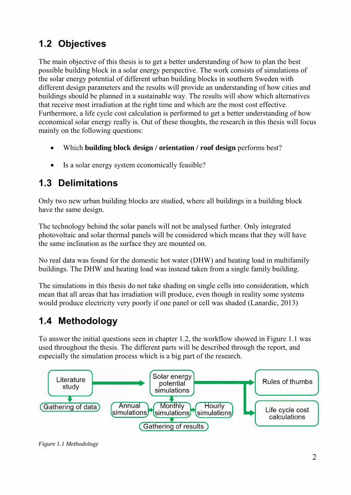
To answer the initial questions seen in chapter 1.2, the workflow showed in Figure 1.1 was used throughout the thesis. The different parts will be described through the report, and especially the simulation process which is a big part of the research.

Figure 1.1 Methodology

4

2 Theoretical framework Solar energy is one of the few possible ways to produce environmentally friendly energy in urban areas. To be able to understand the design and planning process of solar energy there are a few points that have to be understood clearly. This chapter will describe a theoretical framework on the solar potential, the urban planning process, basics behind solar technology and energy requirements.

2.1 Solar energy

In the world, solar energy contributes more and more to the energy grid for each day that goes. For example, Germany reached an installed PV effect of 22 gigawatt in 2012, covering 50% of the country’s midday energy need, equal to 20 nuclear plants for a period during summer (Krishbaum, 2012). However, photovoltaic panels give an uneven production due to the changing weather conditions which make it hard to predict the production. Despite this, solar energy is one of the few ways that you can produce electricity locally and environmentally in urban areas.

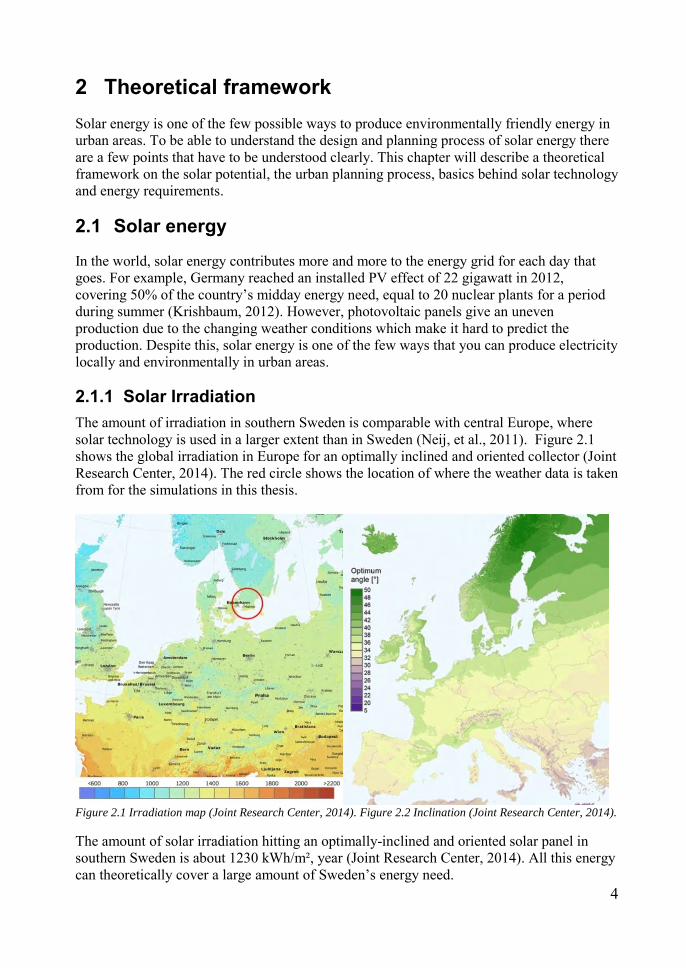
2.1.1 Solar Irradiation The amount of irradiation in southern Sweden is comparable with central Europe, where solar technology is used in a larger extent than in Sweden (Neij, et al., 2011). Figure 2.1 shows the global irradiation in Europe for an optimally inclined and oriented collector (Joint Research Center, 2014). The red circle shows the location of where the weather data is taken from for the simulations in this thesis.

Figure 2.1 Irradiation map (Joint Research Center, 2014). Figure 2.2 Inclination (Joint Research Center, 2014).

The amount of solar irradiation hitting an optimally-inclined and oriented solar panel in southern Sweden is about 1230 kWh/m², year (Joint Research Center, 2014). All this energy can theoretically cover a large amount of Sweden’s energy need.

5

The optimum inclination of solar panels varies depending on where they are located and if there is shading from the surrounding or not. Figure 2.2 shows the variation over Europe. In southern Sweden the optimum inclination is around 40 degrees towards the south which was shown in a simulation made in the Photovoltaic Geographical Information System (PVGIS) (Joint research center, 2009).

2.1.2 Photovoltaic Panels A PV panel produces electricity and consists of multiple solar cells. The solar cells convert energy from sunlight into a flow of electrons. The phenomenon is called the photovoltaic effect, which is when photons of light excite electrons into a higher state of energy, allowing them to act as charge carriers for an electric current (Mr. Solar, 2010).

This was first discovered as early as 1839 by a French experimental physicist, and later Albert Einstein got a Nobel Prize for his theories explaining the effect. However, the photovoltaic panel started to be useful first in the middle of the 20th century with focus on the space program (Bellis, 2013).

There are several types of PV panels, but the most known and used ones are the monocrystalline and the polycrystalline panels. Monocrystalline panels have the highest efficiency of about 15-20%, but are also more expensive.

Figure 2.3 Polycrystalline (Holsinger, 2014) Figure 2.4 Monocrystalline (Damon, 2014)

PV systems can be used either off grid or grid-connected. If the system is not connected to the grid it often has a battery which is able to deliver a more even stream of electricity when there is no sun. If the system is connected to the electricity grid, there is no need for a battery, since the overproduction of electricity will be sent into the grid and used elsewhere (University of Central Florida, 2014).

2.2 Thermal Collectors

Thermal collectors transform solar irradiation into heat by absorbing heat. The heat is transferred from the collector through a medium. In most cases the medium is water, or water with glycol, to make sure it does not freeze.

Solar thermal systems have been around longer than the photovoltaic system, but were forgotten when crude oil was introduced in the industrial revolution. One example of a solar thermal system that reminds of today’s system was introduced in the beginning of the 20th century. It was simply a box painted black, which would slowly heat the water. This system

6

slowly heated the water during day, but the water cooled down rather fast during night, which means that the water could only be used during day (Martinez, 2014).

In 1909, William Bailey introduced a system that looks more like today’s systems, where a collector and a tank were put on the roof. This meant that the water could be kept warm for a longer time, and therefore be used during night.

In the 1950s solar thermal panels became more efficient by introducing the so called selective black surface which was invented in Israel. This is a black colour surface, which gains a big part of the solar irradiation, but does not lose as much heat as a normal black surface.

During the oil crisis in the 1970s, solar thermal systems started to be used to a larger extent, since oil prices went up. This caused the solar thermal panels development to speed up (Renewable energy hub, 2014) .

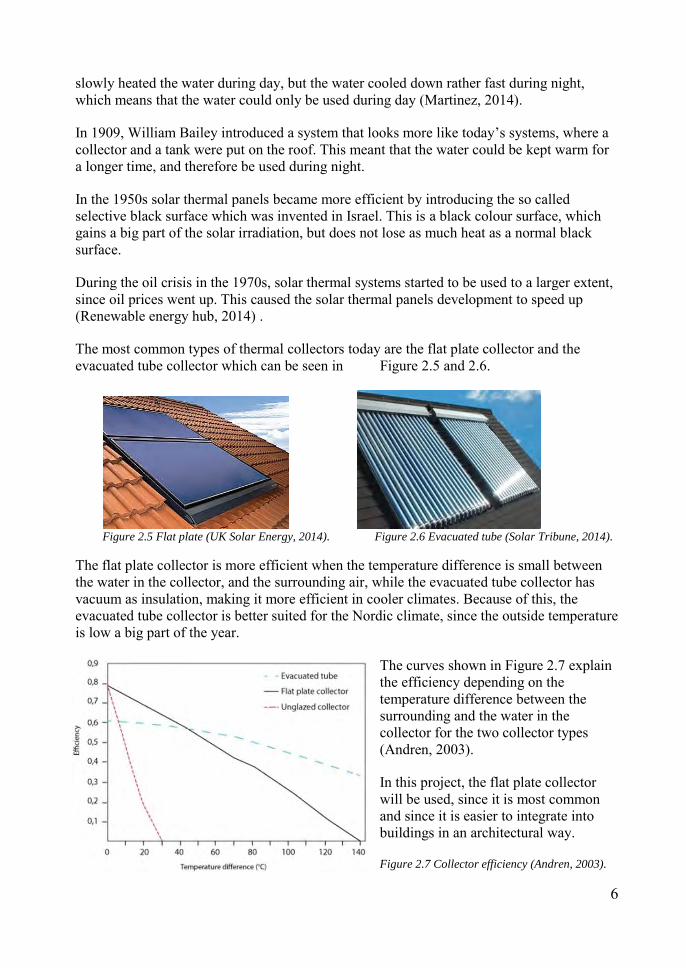
The most common types of thermal collectors today are the flat plate collector and the evacuated tube collector which can be seen in Figure 2.5 and 2.6.

Figure 2.5 Flat plate (UK Solar Energy, 2014). Figure 2.6 Evacuated tube (Solar Tribune, 2014).

The flat plate collector is more efficient when the temperature difference is small between the water in the collector, and the surrounding air, while the evacuated tube collector has vacuum as insulation, making it more efficient in cooler climates. Because of this, the evacuated tube collector is better suited for the Nordic climate, since the outside temperature is low a big part of the year.

The curves shown in Figure 2.7 explain the efficiency depending on the temperature difference between the surrounding and the water in the collector for the two collector types (Andren, 2003).

In this project, the flat plate collector will be used, since it is most common and since it is easier to integrate into buildings in an architectural way.

Figure 2.7 Collector efficiency (Andren, 2003).

7

2.2.1 Shading Shading affects the output of a solar system either if it is a PV or a ST system. A photovoltaic system is much more sensitive to shade than a thermal system. If parts of a photovoltaic system are shaded, it will lower the total system output drastically.

PV panels consist of multiple solar cells, which are connected in series. If one single cell is shaded, it means that all cells produce as much electricity as the shaded cell which is close to zero. In a system of PV panels multiple panels are connected in a so called string or many strings depending on the system’s size. If one cell in one panel is shaded, it means that the whole string’s production is equal to the shaded cell (Andren, 2003).

2.3 Urban density

Cities are getting denser, especially because of the world’s population growth in cities. Cities should not be too dense, since it affects daylight, solar energy, heating need and human health. In the report (Strømann-Andersen & Sttrup, 2011) it is described that the energy load in buildings will increase drastically if the street width is narrower than the buildings height, because this leads to less solar heat gains and daylight, which in turn mean more energy to heat and electrical lighting. However, in this report, these factors will not be investigated further, but it is important to know that many factors contribute to how cities are planned and how they should be planned.

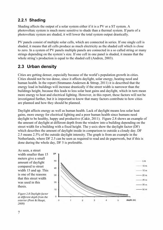
Daylight affects energy as well as human health. Lack of daylight means less solar heat gains, more energy for electrical lighting and a poor human health since humans need daylight to be healthy, happy and productive (Cakir, 2011). Figure 2.8 shows an example of the amount of daylight at different depth from the window into a building depending on the street width for a building with a fixed height. The y-axis show the daylight factor (DF) which describes the amount of daylight inside in comparison to outside a cloudy day. DF 2.5 means 2.5% of the outside daylight intensity. The graph is from an example in the Netherlands, where DF 2.5 can be seen as required to read and do paperwork, but if this is done during the whole day, DF 5 is preferable.

As seen, a street width smaller than 15 meters give a small amount of daylight compared to street width 15 and up. This is one of the reasons that this street width was used in this thesis.

Figure 2.8 Daylight factor

at different depth from the

exterior (Pont & Haupt,

2009)

8

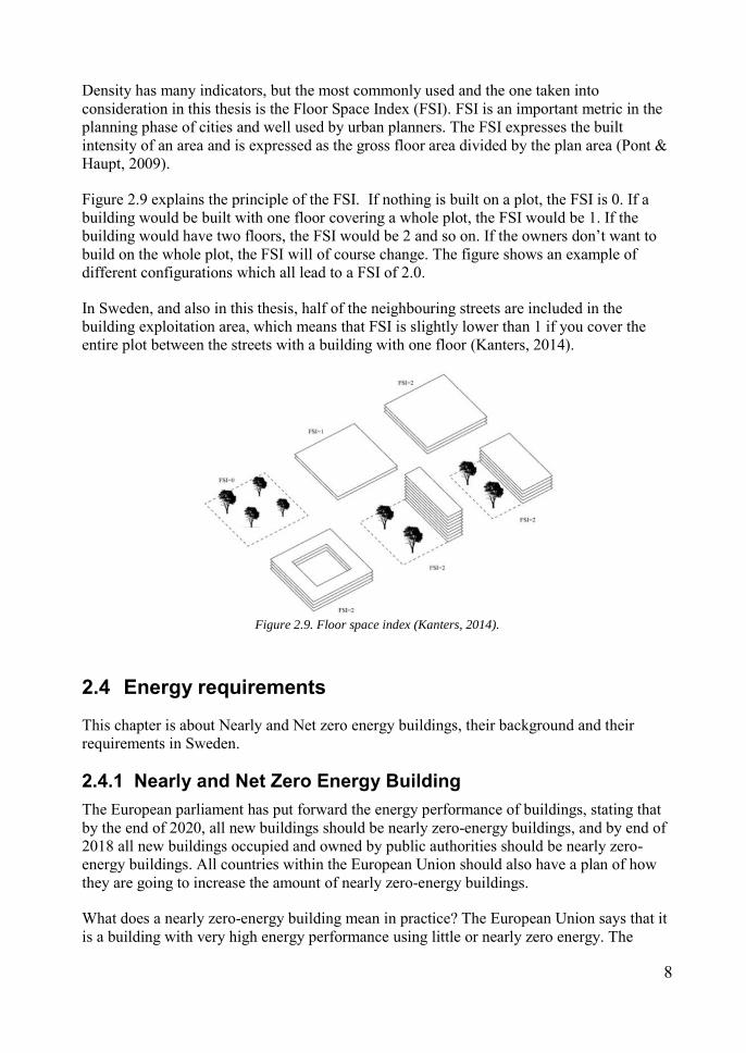
Density has many indicators, but the most commonly used and the one taken into consideration in this thesis is the Floor Space Index (FSI). FSI is an important metric in the planning phase of cities and well used by urban planners. The FSI expresses the built intensity of an area and is expressed as the gross floor area divided by the plan area (Pont & Haupt, 2009).

Figure 2.9 explains the principle of the FSI. If nothing is built on a plot, the FSI is 0. If a building would be built with one floor covering a whole plot, the FSI would be 1. If the building would have two floors, the FSI would be 2 and so on. If the owners don’t want to build on the whole plot, the FSI will of course change. The figure shows an example of different configurations which all lead to a FSI of 2.0.

In Sweden, and also in this thesis, half of the neighbouring streets are included in the building exploitation area, which means that FSI is slightly lower than 1 if you cover the entire plot between the streets with a building with one floor (Kanters, 2014).

Figure 2.9. Floor space index (Kanters, 2014).

2.4 Energy requirements

This chapter is about Nearly and Net zero energy buildings, their background and their requirements in Sweden.

2.4.1 Nearly and Net Zero Energy Building The European parliament has put forward the energy performance of buildings, stating that by the end of 2020, all new buildings should be nearly zero-energy buildings, and by end of 2018 all new buildings occupied and owned by public authorities should be nearly zero-energy buildings. All countries within the European Union should also have a plan of how they are going to increase the amount of nearly zero-energy buildings.

What does a nearly zero-energy building mean in practice? The European Union says that it is a building with very high energy performance using little or nearly zero energy. The

9

energy needed must be covered by a significant amount of renewable sources, including energy produced on-site or nearby. However there is no clear definition of what a nearly zero-energy building is in terms of energy performance. All countries have their own requirements, which mean that some counties will construct buildings with higher performance than others (European Union, 2010).

In this project, the aim is that the examined buildings annually should use as little energy as possible, and locally produce and export as much energy as it imports. A similar definition is called a Net zero-energy building (NZEB), although there is no internationally agreed definition of what a Net zero-energy building is. A NZEB is in most cases seen as a building witch uses zero energy over its life time. For example a building with a very low energy need that produces as much energy as it has uses over its life time. However, some say that you need to include energy for materials, construction of the building (Satori, et al., 2012).

2.4.1.1 FEBY12 requirements FEBY12 is the Swedish voluntary standard that is used to certify Net zero-energy buildings, Passive houses and Mini-energy houses. The reason that there is a Swedish standard is because the German standard is not adapted to the Swedish climate and building regulations. The energy usage allowed in FEBY12 is divided in three climate zones. The further north in Sweden the higher the energy usage is and therefore also a higher energy usage is allowed.

In FEBY12 a NZEB is described as a building that is allowed to use the same amount of energy as a Passive house, if energy is exported in an equal amount to what is imported annually. In the calculation of the imported and exported energy, the energy is weighted, see Appendix 1. The weight depends on the type of energy source for example electricity, how it is produced and what it is used for. This should cover the heating load, cooling load and the common electricity.

FEBY12 defines three different types of heating systems with different energy requirements. The pure heating systems are heating systems without electricity. The non-pure heating / cooling systems have more than one heating & cooling system either with or without electricity. The third system type is heating by only electricity including heat pumps.

For buildings with non-pure heating/cooling systems the energy requirement is balanced by using a simple formula which can be found in Appendix 1 (Sveriges Centrum för Nollenergihus, 2012).

2.4.1.2 BBR 20 requirements The Swedish National Board of Housing, Building and Planning issues the latest Swedish building regulations (BBR 20), including energy requirements (Boverket, 2013).

These requirements are what Sweden proposed to be called Nearly zero-energy standards. However, this standard allows considerable more energy to be used in buildings than for example FEBY12. BBRs latest standard has been criticised by many, including the Swedish Energy Agency (Energimyndigheten) because technology and knowledge to build low energy buildings has existed for a long time in Sweden. Because of this critique a new proposal will be introduced in 2015.

10

To be allowed to construct a new building in Sweden today; the requirements of BBR 20 have to be attained. In BBR there are two different energy requirements depending on if the building is heated with or without electricity (Boverket, 2013).

2.4.1.3 Comparison of requirements When comparing the two standards FEBY12 and BBR for residential buildings, there is a drastic difference. The energy demand in BBR is allowed to be 43-120% higher than what is allowed in FEBY depending on the type of heating system in the building.

In the analyses made in this report the pure heating system’s energy requirements in FEBY12 will be used, since the buildings are presupposed to be heated by district heat and solar energy.

Figure 2.10 shows all the requirements for residential buildings. The DHW usage normally is about 25 kWh/m²a and the building electricity is 15 kWh/m²a (SVEBY, 2009). These values are shown in the graph in the BBR requirements. The energy requirement of FEBY12 for non-pure heating systems is an example, which can be higher or lower depending on the electricity usage since there is a formula in the requirement weighting the different energy sources.

For the passive houses in this thesis, values were taken from four passive house projects in Sweden; 10 kWh/m²a for building electricity (Janson, 2010), and the same DHW load of 25 kWh/m²a (SVEBY, 2009). As seen in graph 2.2 this means that the heating load for the FEBY12 non-pure heating system is 28 kWh/m²a.

To produce enough electricity and heat to reach the NZEB reference values, the PV-panels have to produce 10 kWh/m²a and the ST-panels 40 kWh/m²a, meaning per square meter building floor area2.

Figure 2.10 Energy requirements.

2 If the buildings floor area is 100 m², the total production of the PV-system has to be 1000 kWh/year. 1000kWh/a / 100m² =10

kWh/m²a.

0

25

50

75

100

FEBY 12 BBR 20 FEBY 12 BBR 20 FEBY 12 BBR 20

non-pure heating system pure heating system heating with electricity

Ener

gy u

se /

(kW

h/m

²a)

Electricity DHW Heating

11

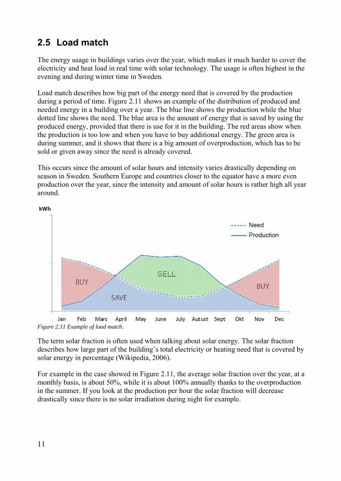
2.5 Load match

The energy usage in buildings varies over the year, which makes it much harder to cover the electricity and heat load in real time with solar technology. The usage is often highest in the evening and during winter time in Sweden.

Load match describes how big part of the energy need that is covered by the production during a period of time. Figure 2.11 shows an example of the distribution of produced and needed energy in a building over a year. The blue line shows the production while the blue dotted line shows the need. The blue area is the amount of energy that is saved by using the produced energy, provided that there is use for it in the building. The red areas show when the production is too low and when you have to buy additional energy. The green area is during summer, and it shows that there is a big amount of overproduction, which has to be sold or given away since the need is already covered.

This occurs since the amount of solar hours and intensity varies drastically depending on season in Sweden. Southern Europe and countries closer to the equator have a more even production over the year, since the intensity and amount of solar hours is rather high all year around.

Figure 2.11 Example of load match.

The term solar fraction is often used when talking about solar energy. The solar fraction describes how large part of the building’s total electricity or heating need that is covered by solar energy in percentage (Wikipedia, 2006).

For example in the case showed in Figure 2.11, the average solar fraction over the year, at a monthly basis, is about 50%, while it is about 100% annually thanks to the overproduction in the summer. If you look at the production per hour the solar fraction will decrease drastically since there is no solar irradiation during night for example.

12

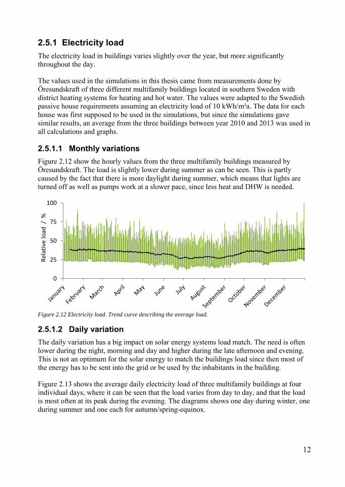
2.5.1 Electricity load The electricity load in buildings varies slightly over the year, but more significantly throughout the day.

The values used in the simulations in this thesis came from measurements done by Öresundskraft of three different multifamily buildings located in southern Sweden with district heating systems for heating and hot water. The values were adapted to the Swedish passive house requirements assuming an electricity load of 10 kWh/m²a. The data for each house was first supposed to be used in the simulations, but since the simulations gave similar results, an average from the three buildings between year 2010 and 2013 was used in all calculations and graphs.

2.5.1.1 Monthly variations Figure 2.12 show the hourly values from the three multifamily buildings measured by Öresundskraft. The load is slightly lower during summer as can be seen. This is partly caused by the fact that there is more daylight during summer, which means that lights are turned off as well as pumps work at a slower pace, since less heat and DHW is needed.

Figure 2.12 Electricity load. Trend curve describing the average load.

2.5.1.2 Daily variation The daily variation has a big impact on solar energy systems load match. The need is often lower during the night, morning and day and higher during the late afternoon and evening. This is not an optimum for the solar energy to match the buildings load since then most of the energy has to be sent into the grid or be used by the inhabitants in the building.

Figure 2.13 shows the average daily electricity load of three multifamily buildings at four individual days, where it can be seen that the load varies from day to day, and that the load is most often at its peak during the evening. The diagrams shows one day during winter, one during summer and one each for autumn/spring-equinox.

0

25

50

75

100

Rel

ativ

e lo

ad /

%

13

Figure 2.13 Daily electricity load.

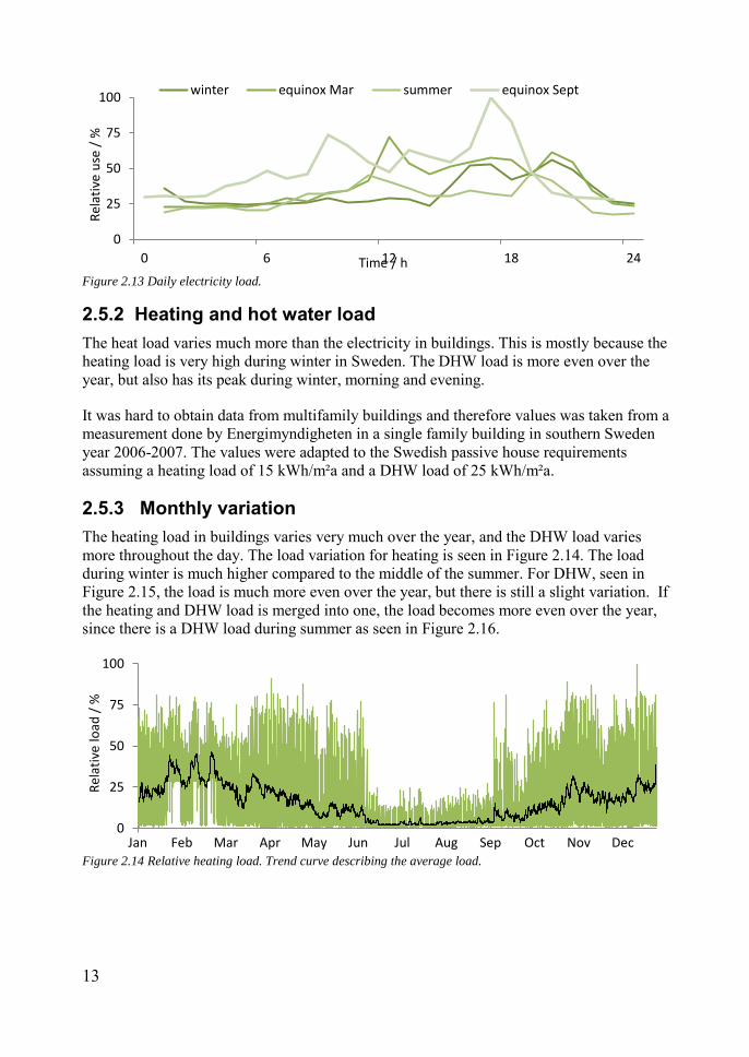
2.5.2 Heating and hot water load The heat load varies much more than the electricity in buildings. This is mostly because the heating load is very high during winter in Sweden. The DHW load is more even over the year, but also has its peak during winter, morning and evening.

It was hard to obtain data from multifamily buildings and therefore values was taken from a measurement done by Energimyndigheten in a single family building in southern Sweden year 2006-2007. The values were adapted to the Swedish passive house requirements assuming a heating load of 15 kWh/m²a and a DHW load of 25 kWh/m²a.

2.5.3 Monthly variation The heating load in buildings varies very much over the year, and the DHW load varies more throughout the day. The load variation for heating is seen in Figure 2.14. The load during winter is much higher compared to the middle of the summer. For DHW, seen in Figure 2.15, the load is much more even over the year, but there is still a slight variation. If the heating and DHW load is merged into one, the load becomes more even over the year, since there is a DHW load during summer as seen in Figure 2.16.

Figure 2.14 Relative heating load. Trend curve describing the average load.

0

25

50

75

100

0 6 12 18 24

Rel

ativ

e u

se /

%

Time / h

winter equinox Mar summer equinox Sept

0

25

50

75

100

Jan Feb Mar Apr May Jun Jul Aug Sep Oct Nov Dec

Rel

ativ

e lo

ad /

%

14

Figure 2.15 Relative DHW load.

Figure 2.16 Relative total heat load.

2.5.3.1 Daily variation The daily variation for heating is small over a day. There is often a more constant heat load during winter, and close to zero during summer. Hot water however varies more over the day, as seen in Figure 2.17.The load these specific days seem to be highest between 12-24h.

Figure 2.17 Daily DHW load.

0

25

50

75

100


Rel

ativ

e lo

ad /

%

0

25

50

75

100


Rel

ativ

e lo

ad /

%

0

25

50

75

100

1 7 13 19

Rel

lati

ve u

se /

%

Time / h

winter equinox Sept summer equinox Mar

15

2.5.3.2 Seasonal Storage and District Heat To be able to produce and utilise more heat than needed during summer, you need to either store the heat to be used later when needed, or you have to send the overproduction into the district heating system, and when there is a need, buy heat from the district heating company.

There are a few examples where the heat is stored in the ground. One example that was surprisingly successful is The Drake Landing Solar Community in Okotoks, Alberta Canada. 52 single family houses with flat plate thermal collectors were connected to an insulated bore hole storage in the ground. The system had the target to achieve more than 90% solar fraction at its fifth year of operation, but it got as high as 97%.

The efficiency of this storage was only 6% the first year, which means that 94% of the heat is lost into the ground. The reason for this is that it takes a long time to increase the temperature of a big amount of soil in the ground. The efficiency increased every year until year four when it was as high as 54% but decreased a bit year five to 36% (Sibbitt, et al., 2012).

A bore hole storage will not be considered in this report, since there is only a limited amount of space in cities, and therefore it’s hard to find the space for a underground storage of heat. There are also already well distributed district heating system in most cities, which mean that it is easier to connect the building to the district heating system instead of creating an underground storage for heat.

There is a heat exchanger between the solar collector loop and the district heating system, which only exchange heat when the produced heat has a certain temperature. In most cases about 75 C° which is hard to achieve in ST-systems in Swedish conditions. This means that a big part of the overproduced heat cannot be sent into such district heating systems, and is therefore lost. To produce heat at a high temperature it is important that the collectors have the right inclination and orientation.

About twenty solar energy systems connected to a district heating system were installed between year 2000 and 2010 in Sweden. These were evaluated in the report “Solvärme I fjärrvärmenätet”, and it shows that heat from solar collectors produce as little as 200 kWh/m²a in some cases in Malmö. This means that it has not been economically feasible in many cases while it is possible to reach much higher values and therefore make it more economical. Collectors connected to district heating in Denmark for example have a production of about 400 kWh/m², collector (Dalenbäck, et al., 2013).

16

2.6 State of the art for solar urban planning

The solar energy potential of four different building blocks that are commonly seen in Swedish cities were analysed in a research project (Kanters, 2014) at LTH, Energy and Building design. The simulations show that some building block designs are better suited for production of solar energy than others. The analysed designs are shown in Figure 2.18.

The closed building block seems to receive the most solar energy in many cases and the strips building block receive the least energy in all cases compared to its floor area. Only two roof types were analysed, a flat roof and a gable roof. The buildings with flat roof seems to always receive a higher amount of irradiation, while the gable roof receives a higher amount of irradiation on one side of the roof and almost none on the side facing away from the sun. Because of shading on one side of the gable roof, and shading on the facades caused by this high roof these buildings receive significantly less solar irradiation than the buildings with flat roofs.

The simulations show that it is possible to produce enough energy to cover the buildings’ need annually with a floor space index up to 2.5 for some building types. However, a few alternatives are possible to produce enough energy when the FSI is 2.5. Therefore, in this thesis the floor space index will be fixed at 2.0, which will give more flexibility in the design process (Kanters, 2014).

Figure 2.18 Building block designs (Kanters, 2014).

18

3 Method This chapter describes the workflow, simulation software, different parameters and settings used within this thesis.

The simulations are performed to investigate several design parameters. Furthermore, the simulations will examine if it is possible to develop a suitable shape for the roof. Shading should for example be avoided as far as possible, and a good inclination for the roof surfaces is important to maximize the production.

3.1 Simulation software

The Irradiation analysis will be made with the 3d modelling tool Rhinoceros 3D 5 (Rhino).

First a building is modelled in Rhino. Within Rhino the plugin Grasshopper is used to multiply the building into a building block and to conduct a parametric study where multiple parameters are changed, such as the orientation and roof inclination. Grasshopper is a plugin that makes it possible to write a script that decides how the model will look in Rhino.

In Grasshopper another plugin called DIVA4Rhino (DIVA) is used to measure the solar irradiation on the building blocks roofs and facades. DIVA is a simulation plugin which makes it possible to conduct irradiation, thermal and daylight analysis.

Within DIVA, two different components are used to calculate the solar irradiation. One component with the name Radiance, which is commonly used will be used for most simulations, but can unfortunately not display its results per hour. Therefore another component within DIVA called Energy+ will be used for the simulation when a result per hour is needed. The workflow can be seen in Figure 3.1 (Jakubiec & Reinhart, 2011).

Figure 3.1 Simulation process.

19

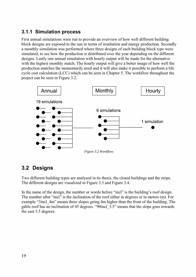
3.1.1 Simulation process First annual simulations were run to provide an overview of how well different building block designs are exposed to the sun in terms of irradiation and energy production. Secondly a monthly simulation was performed where three designs of each building block type were simulated, to see how the production is distributed over the year depending on the different designs. Lastly one annual simulation with hourly output will be made for the alternative with the highest monthly match. The hourly output will give a better image of how well the production matches the momentarily need and it will also make it possible to perform a life cycle cost calculation (LCC) which can be seen in Chapter 5. The workflow throughout the project can be seen in Figure 3.2.

Figure 3.2 Workflow.

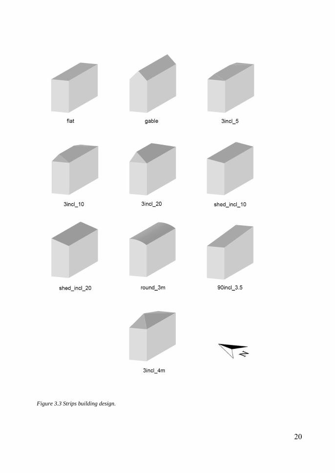
3.2 Designs

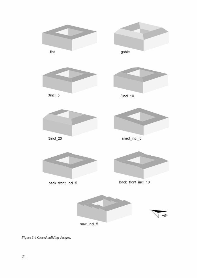
Two different building types are analysed in tis thesis, the closed buildings and the strips. The different designs are visualized in Figure 3.3 and Figure 3.4.

In the name of the design, the number or words before “incl” is the building’s roof design. The number after “incl” is the inclination of the roof either in degrees or in meters (m). For example “3incl_4m” means three slopes going 4m higher than the front of the building. The gable roof has an inclination of 45 degrees. “90incl_3.5” means that the slope goes towards the east 3.5 degrees.

20

Figure 3.3 Strips building design.

21

Figure 3.4 Closed building designs.

22

3.3 Parameters and settings

There are a variety of parameters that are considered in the analyses made and also multiple settings within the software that are used for the daylight simulations made.

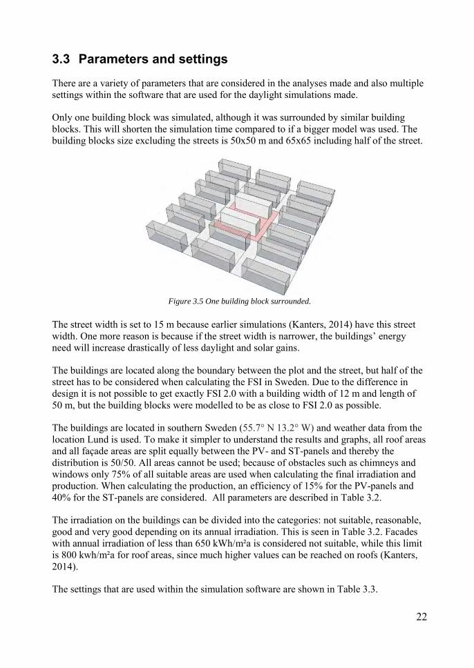
Only one building block was simulated, although it was surrounded by similar building blocks. This will shorten the simulation time compared to if a bigger model was used. The building blocks size excluding the streets is 50x50 m and 65x65 including half of the street.

Figure 3.5 One building block surrounded.

The street width is set to 15 m because earlier simulations (Kanters, 2014) have this street width. One more reason is because if the street width is narrower, the buildings’ energy need will increase drastically of less daylight and solar gains.

The buildings are located along the boundary between the plot and the street, but half of the street has to be considered when calculating the FSI in Sweden. Due to the difference in design it is not possible to get exactly FSI 2.0 with a building width of 12 m and length of 50 m, but the building blocks were modelled to be as close to FSI 2.0 as possible.

The buildings are located in southern Sweden (55.7° N 13.2° W) and weather data from the location Lund is used. To make it simpler to understand the results and graphs, all roof areas and all façade areas are split equally between the PV- and ST-panels and thereby the distribution is 50/50. All areas cannot be used; because of obstacles such as chimneys and windows only 75% of all suitable areas are used when calculating the final irradiation and production. When calculating the production, an efficiency of 15% for the PV-panels and 40% for the ST-panels are considered. All parameters are described in Table 3.2.

The irradiation on the buildings can be divided into the categories: not suitable, reasonable, good and very good depending on its annual irradiation. This is seen in Table 3.2. Facades with annual irradiation of less than 650 kWh/m²a is considered not suitable, while this limit is 800 kwh/m²a for roof areas, since much higher values can be reached on roofs (Kanters, 2014).

The settings that are used within the simulation software are shown in Table 3.3.

23

Table 3.1 Used parameters.

Location

southern Sweden Orientation from the south 0, 15, 30, 45, 60, 75 degrees

Plot excl. street 50 x 50 m

incl. street 65 x 65 m

Street width

15 m

Number of plots 3 x 3

Strips

building designs 10

Width between buildings 26 m

height 21 m

FSI 1.99

Closed

building designs 9 courtyard 26 m

height 15 m

FSI 2.16

Efficiency PV 15 %

ST 40 %

Area PV/ST 50/50 %

Usable area 75 %

Table 3.2 Suitable areas.

Roof / kWh/m²a Suitable

Not suitable Reasonable Good Very good

<800 800-899 900-1019 1020<

Facade / kWh/m²a Suitable

Not suitable Reasonable Good Very good

<650 650-899 900-1019 1020<

24

Table 3.3 Inputs into Diva4rhino.

Weather data Lund, Sweden

Model

building types strips & closed

Plot, excl. streets 50 x 50 m

number of plots 3 x 3

street width 15 m

floor space index 2.0

building depth 12 m

floor height 3 m

Reflectance ground 20 %

buildings 35 %

Radiance settings

grid size 1x1 m

ambient bounces 3

ambient divisions 2048

ambient super-samples 20

ambient resolution 500

ambient accuracy 0.1

26

4 Results In this chapter the results can be visualised in graphs with describing texts for different buildings and building block designs.

4.1 Annual simulations

In this chapter the annual simulations are described. Ten different design alternatives for the strips and nine for the closed building block are analysed. Different graphs are produced to explain the different outputs from all simulations. The graphs show the production, the average irradiation and the suitable areas for the roof and facade.

Figure 3.6 -3.7 and 3.13- 3.14 shows the PV/ST production divided by the building’s floor area. This is done to be able to compare the results from the strips and closed building types to see which one performs best in relation to the energy requirements in FEBY12. The average irradiation gives an understanding of how well the surfaces are located, compared to how much they could produce. In the graphs describing the suitable areas, you can see how big part of the area that is on the roof and on the façade. In these figures there is a line labelled NZEB. This line describes the amount of annual production needed to produce enough heat or electricity to meet the buildings annual need, which is 10 kWh/m²a for electricity and 40 kWh/m²a for heat. This is described in more detail in chapter 2.3.1.3.

Figure 3.8-3.10 and 3.15-3.17 shows the production, average irradiation and suitable areas divided between the roof and the façade. There are six stacks for each building, representing the different orientations 0, 15, 30, 45, 60 and 75.

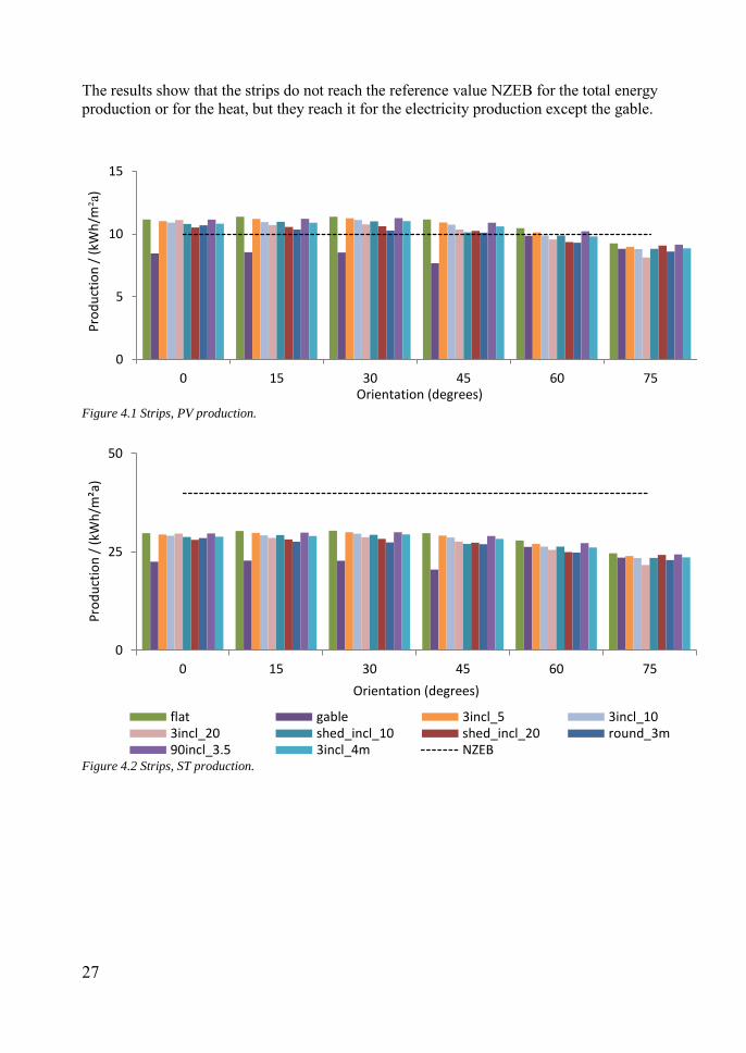
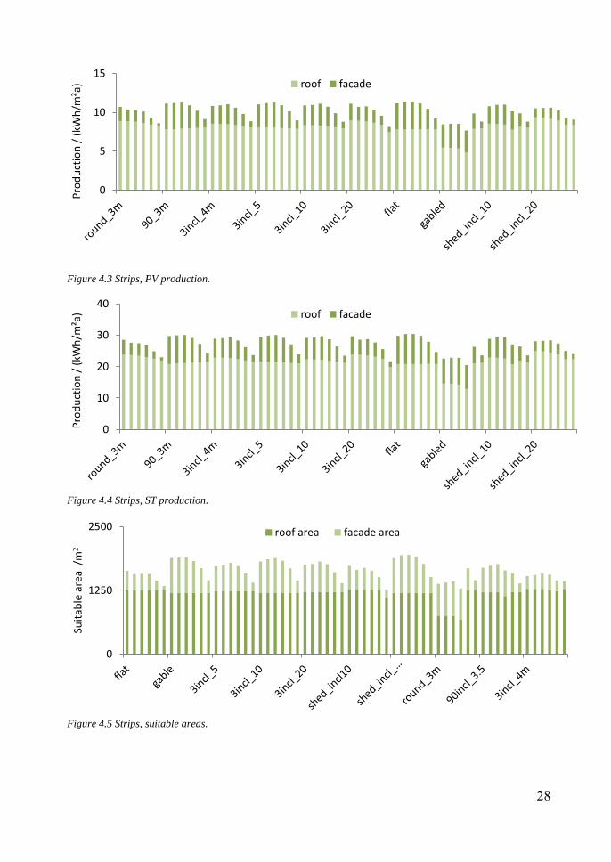
4.1.1 Strips The different designs shown in Figure 4.1 and Figure 4.2 follow the same trend with respect to the orientation. The difference is small, but the result is slightly worse the more the building is rotated from the south. The optimum orientation in most cases seems to be 30 degrees from the south, but it varies slightly between all alternatives. The gable roof does not follow the trend and instead the optimum orientation is 60 degrees from the south. The production for the gable roof is still lower than most other alternatives in all directions since a big part of the roof is always shaded.

In Figure 4.3 and Figure 4.4 the production on the roof and on the facade is divided into two stacks on top of each other to be able to analyse the different outputs. For all designs, there is six stacks, each showing the results for each orientation, 0-75 degrees. As expected the roof always has a higher production. Most of the roofs’ optimum orientation is towards the south except for the gable roof which has its highest production 60 degrees from the south. The façades’ highest production is 30 degrees from south except for the round_3m, which is towards the south.

Figure 4.5 shows how the suitable roof and façade area varies depending on orientation. There is almost no façade utilized when the buildings are oriented 75 degrees from the south. The size of the utilized façade area is one of the reasons why the production varies with the orientation of the buildings.

27

The results show that the strips do not reach the reference value NZEB for the total energy production or for the heat, but they reach it for the electricity production except the gable.

Figure 4.1 Strips, PV production.

Figure 4.2 Strips, ST production.

0

5

10

15

0 15 30 45 60 75

Pro

du

ctio

n /

(kW

h/m

²a)

Orientation (degrees)

0

25

50

0 15 30 45 60 75

Pro

du

ctio

n /

(kW

h/m

²a)


flat gable 3incl_5 3incl_103incl_20 shed_incl_10 shed_incl_20 round_3m90incl_3.5 3incl_4m NZEB

28


Figure 4.4 Strips, ST production.

Figure 4.5 Strips, suitable areas.

0

5

10

15P

rod

uct

ion

/ (

kWh

/m²a

) roof facade

0

10

20

30

40

Pro

du

ctio

n /

(kW

h/m

²a) roof facade

0

1250

2500

Suit

able

are

a /

m2

roof area facade area

29

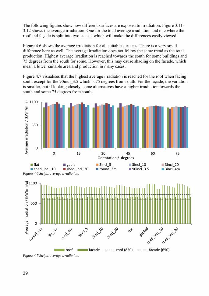
The following figures show how different surfaces are exposed to irradiation. Figure 3.11-3.12 shows the average irradiation. One for the total average irradiation and one where the roof and façade is split into two stacks, which will make the differences easily viewed.

Figure 4.6 shows the average irradiation for all suitable surfaces. There is a very small difference here as well. The average irradiation does not follow the same trend as the total production. Highest average irradiation is reached towards the south for some buildings and 75 degrees from the south for some. However, this may cause shading on the facade, which mean a lower suitable area and production in many cases.

Figure 4.7 visualises that the highest average irradiation is reached for the roof when facing south except for the 90incl_3.5 which is 75 degrees from south. For the façade, the variation is smaller, but if looking closely, some alternatives have a higher irradiation towards the south and some 75 degrees from south.

Figure 4.6 Strips, average irradiation.


0

550

1100

0 15 30 45 60 75Ave

rage

irra

dia

tio

n /

(kW

h/m

²a)

Orientation / degrees

flat gable 3incl_5 3incl_10 3incl_20shed_incl_10 shed_incl_20 round_3m 90incl_3.5 3incl_4m

0

550

1100

Ave

rage

irra

dia

tio

n /

(kW

h/m

²a)

roof facade roof (850) facade (650)

30

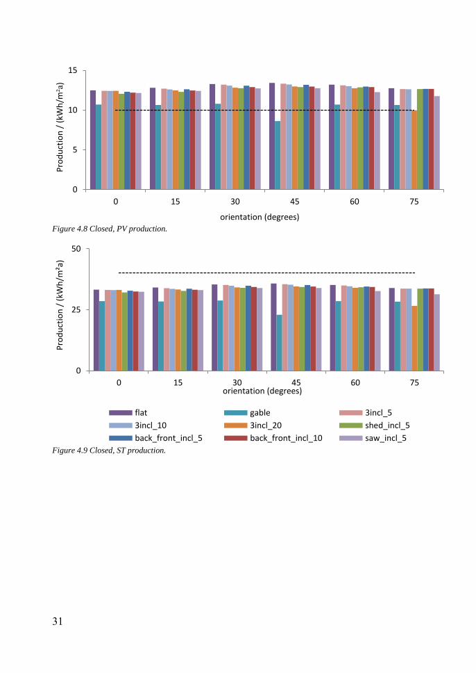
4.1.2 Closed building block For the closed building block the optimum orientation is 45 degrees from the south in most cases while the gable roof is outside the trend. The optimum orientation for the gable roof is instead 30 and 60 degrees from the south, but the production is still lower than all other alternatives due to shading on a big part of the roof and facade. This can be seen in Figure 4.8 and Figure 4.9.

When splitting the production between the roof and the façade, seen in Figure 4.10 and Figure 4.11, it shows that the roof has its highest production when the building is oriented towards the south in all cases. In all cases the façades’ highest production is when the building is oriented 45 degrees from the south.

The variations of production for the roof do not differ as much in respect to the orientation as for the façade. Therefore it will be the façade production that regulates how the building should be oriented. If the facade is not utilized, the building will always perform better towards the south except the gable roof which has its highest production towards the south as well as 15 and 75 degrees from the south.

As seen in Figure 4.12 the suitable areas do not differ as much for the closed buildings as for the strips. The available roof area is bigger for the closed buildings, but just a small part of the façade is suitable for solar energy production for most designs.

Results show that the Closed building block do not reach the reference value NZEB for the heat production, but nearly all reach it for the electricity production. However, this building type performs better than the Strips.

31

Figure 4.8 Closed, PV production.

Figure 4.9 Closed, ST production.

0

5

10

15

0 15 30 45 60 75

Pro

du

ctio

n /

(kW

h/m

²a)

orientation (degrees)

0

25

50

0 15 30 45 60 75

Pro

du

ctio

n /

(kW

h/m

²a)

orientation (degrees)

flat gable 3incl_5

3incl_10 3incl_20 shed_incl_5

back_front_incl_5 back_front_incl_10 saw_incl_5

32



Figure 4.12 Closed, suitable areas.

0

5

10

15P

rod

uct

ion

/ (

kWh

/m²a

) roof facade

0

10

20

30

40

Pro

du

ctio

n /

(kW

h/m

²a)

roof facade

0

1250

2500

Suit

able

are

a /

m2

roof area facade area

33

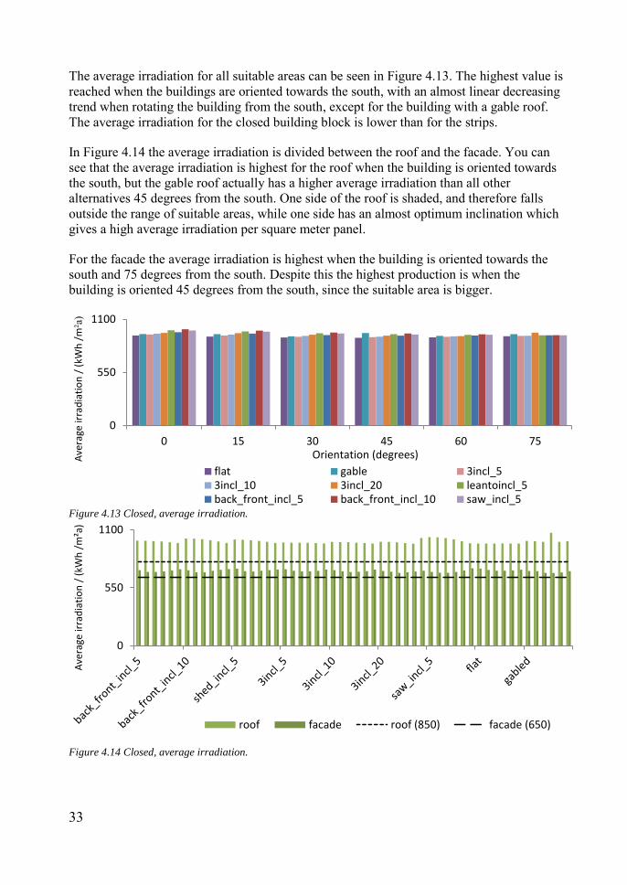
The average irradiation for all suitable areas can be seen in Figure 4.13. The highest value is reached when the buildings are oriented towards the south, with an almost linear decreasing trend when rotating the building from the south, except for the building with a gable roof. The average irradiation for the closed building block is lower than for the strips.

In Figure 4.14 the average irradiation is divided between the roof and the facade. You can see that the average irradiation is highest for the roof when the building is oriented towards the south, but the gable roof actually has a higher average irradiation than all other alternatives 45 degrees from the south. One side of the roof is shaded, and therefore falls outside the range of suitable areas, while one side has an almost optimum inclination which gives a high average irradiation per square meter panel.

For the facade the average irradiation is highest when the building is oriented towards the south and 75 degrees from the south. Despite this the highest production is when the building is oriented 45 degrees from the south, since the suitable area is bigger.

Figure 4.13 Closed, average irradiation.


0

550

1100

0 15 30 45 60 75

Ave

rage

irra

dia

tio

n /

(kW

h /

m²a

)


flat gable 3incl_53incl_10 3incl_20 leantoincl_5back_front_incl_5 back_front_incl_10 saw_incl_5

0

550

1100

Ave

rage

irra

dia

tio

n /

(kW

h /

m²a

)

roof facade roof (850) facade (650)

34

4.2 Monthly simulations

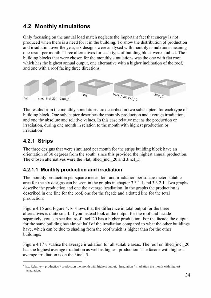
Only focussing on the annual load match neglects the important fact that energy is not produced when there is a need for it in the building. To show the distribution of production and irradiation over the year, six designs were analysed with monthly simulations meaning one result per month. Three alternatives for each type of building block were studied. The building blocks that were chosen for the monthly simulations was the one with flat roof which has the highest annual output, one alternative with a higher inclination of the roof, and one with a roof facing three directions.

The results from the monthly simulations are described in two subchapters for each type of building block. One subchapter describes the monthly production and average irradiation, and one the absolute and relative values. In this case relative means the production or irradiation, during one month in relation to the month with highest production or irradiation3.

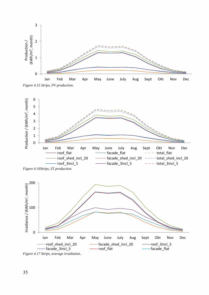
4.2.1 Strips The three designs that were simulated per month for the strips building block have an orientation of 30 degrees from the south, since this provided the highest annual production. The chosen alternatives were the Flat, Shed_incl_20 and 3incl_5.

4.2.1.1 Monthly production and irradiation The monthly production per square meter floor and irradiation per square meter suitable area for the six designs can be seen in the graphs in chapter 3.3.1.1 and 3.3.2.1. Two graphs describe the production and one the average irradiation. In the graphs the production is described in one line for the roof, one for the façade and a dotted line for the total production.

Figure 4.15 and Figure 4.16 shows that the difference in total output for the three alternatives is quite small. If you instead look at the output for the roof and facade separately, you can see that roof_incl_20 has a higher production. For the facade the output for the same building has almost half of the irradiation compared to what the other buildings have, which can be due to shading from the roof which is higher than for the other buildings.

Figure 4.17 visualise the average irradiation for all suitable areas. The roof on Shed_incl_20 has the highest average irradiation as well as highest production. The facade with highest average irradiation is on the 3incl_5. 3 Ex. Relative = production / production the month with highest output. | Irradiation / irradiation the month with highest

irradiation.

35


Figure 4.16Strips, ST production.


0

1

2

3

Jan Feb Mar Apr May June July Aug Sept Okt Nov Dec

Pro

du

ctio

n /

(

kWh

/m²,

mo

nth

)

0

1

2

3

4

5

6

Jan Feb Mar Apr May June July Aug Sept Okt Nov DecPro

du

ctio

n /

(kW

h/m

², m

on

th)

roof_flat facade_flat total_flat

roof_shed_incl_20 facade_shed_incl_20 total_shed_incl_20

roof_3incl_5 facade_3incl_5 total_3incl_5

0

100

200


Irra

dia

nce

/ (

kWh

/m²,

mo

nth

)

roof_shed_incl_20 facade_shed_incl_20 roof_3incl_5facade_3incl_5 roof_flat facade_flat

36

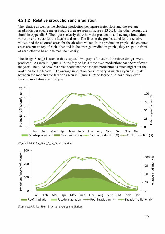
4.2.1.2 Relative production and irradiation The relative as well as the absolute production per square meter floor and the average irradiation per square meter suitable area are seen in figure 3.23-3.24. The other designs are found in Appendix 3. The figures clearly show how the production and average irradiation varies over the year for the façade and roof. The lines in the graphs stand for the relative values, and the coloured areas for the absolute values. In the production graphs, the coloured areas are put on top of each other and in the average irradiation graphs, they are put in front of each other to be able to read them easily.

The design 3incl_5 is seen in this chapter. Two graphs for each of the three designs were produced. As seen in Figure 4.18 the façade has a more even production than the roof over the year. The filled coloured areas show that the absolute production is much higher for the roof than for the facade. The average irradiation does not vary as much as you can think between the roof and the façade as seen in Figure 4.19 the façade also has a more even average irradiation over the year.

Figure 4.18 Strips_3incl_5_or_30, production.

Figure 4.19 Strips_3incl_5_or_45, average irradiation.

0

25

50

75

100

0

10

20

30

40


Rel

ativ

e p

rod

uct

ion

/ %

Pro

du

ctio

n /

(kW

h/m

2, m

on

th)

Facade production Roof production Facade production (%) Roof production (%)

0

25

50

75

100

0

100

200

300


Rel

ativ

e ir

rad

iati

on

/ %

Irra

dia

tio

n /

(kW

h/m

2, m

on

th)

Roof irradiation Facade irradiation Roof irradiation (%) Facade irradiation (%)

37

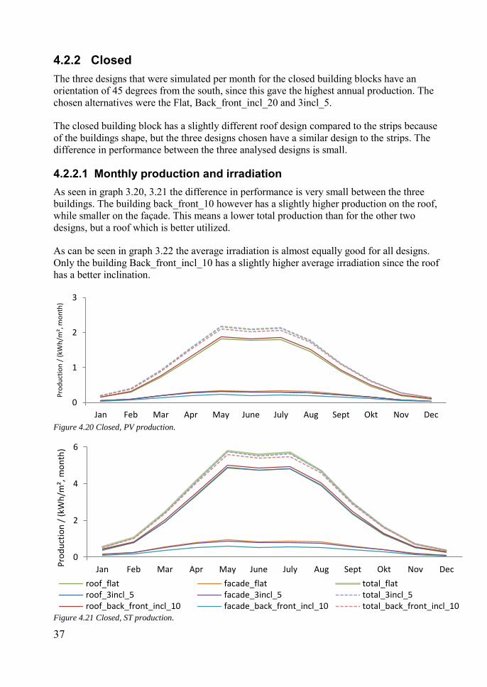
4.2.2 Closed The three designs that were simulated per month for the closed building blocks have an orientation of 45 degrees from the south, since this gave the highest annual production. The chosen alternatives were the Flat, Back_front_incl_20 and 3incl_5.

The closed building block has a slightly different roof design compared to the strips because of the buildings shape, but the three designs chosen have a similar design to the strips. The difference in performance between the three analysed designs is small.

4.2.2.1 Monthly production and irradiation As seen in graph 3.20, 3.21 the difference in performance is very small between the three buildings. The building back_front_10 however has a slightly higher production on the roof, while smaller on the façade. This means a lower total production than for the other two designs, but a roof which is better utilized.

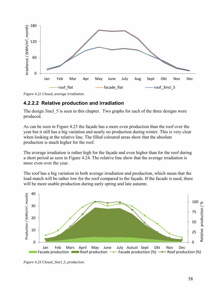
As can be seen in graph 3.22 the average irradiation is almost equally good for all designs. Only the building Back_front_incl_10 has a slightly higher average irradiation since the roof has a better inclination.



0

1

2

3


Pro

du

ctio

n /

(kW

h/m

², m

on

th)

0

2

4

6


Pro

du

ctio

n /

(kW

h/m

², m

on

th)

roof_flat facade_flat total_flatroof_3incl_5 facade_3incl_5 total_3incl_5roof_back_front_incl_10 facade_back_front_incl_10 total_back_front_incl_10

38


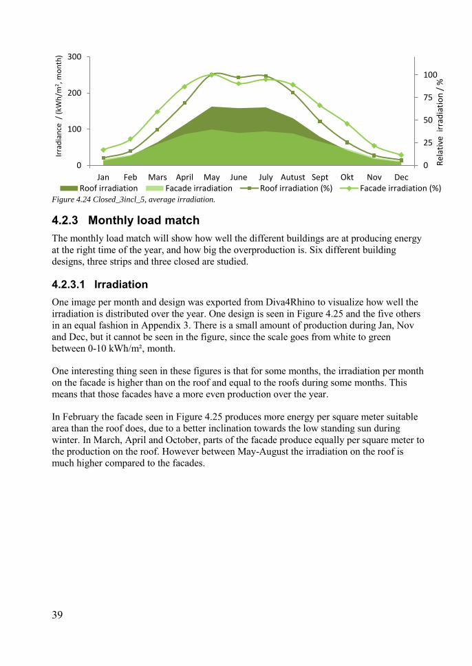
4.2.2.2 Relative production and irradiation The design 3incl_5 is seen in this chapter. Two graphs for each of the three designs were produced.

As can be seen in Figure 4.23 the façade has a more even production than the roof over the year but it still has a big variation and nearly no production during winter. This is very clear when looking at the relative line. The filled coloured areas show that the absolute production is much higher for the roof.

The average irradiation is rather high for the façade and even higher than for the roof during a short period as seen in Figure 4.24. The relative line show that the average irradiation is more even over the year.

The roof has a big variation in both average irradiation and production, which mean that the load match will be rather low for the roof compared to the façade. If the facade is used, there will be more usable production during early spring and late autumn.

Figure 4.23 Closed_3incl_5, production.

0

60

120

180


Irra

dia

nce

/ (

kWh

/m²,

mo

nth

)

roof_flat facade_flat roof_3incl_5

0

25

50

75

100

0

10

20

30

40

Jan Feb Mars April May June July Autust Sept Okt Nov Dec

Rel

ativ

e p

rod

uct

ion

/ %

Pro

du

ctio

n /

(kW

h/m

2 , m

on

th)


39

Figure 4.24 Closed_3incl_5, average irradiation.

4.2.3 Monthly load match The monthly load match will show how well the different buildings are at producing energy at the right time of the year, and how big the overproduction is. Six different building designs, three strips and three closed are studied.

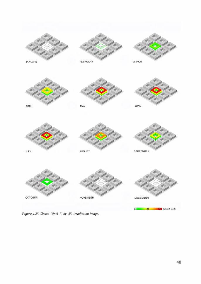
4.2.3.1 Irradiation One image per month and design was exported from Diva4Rhino to visualize how well the irradiation is distributed over the year. One design is seen in Figure 4.25 and the five others in an equal fashion in Appendix 3. There is a small amount of production during Jan, Nov and Dec, but it cannot be seen in the figure, since the scale goes from white to green between 0-10 kWh/m², month.

One interesting thing seen in these figures is that for some months, the irradiation per month on the facade is higher than on the roof and equal to the roofs during some months. This means that those facades have a more even production over the year.

In February the facade seen in Figure 4.25 produces more energy per square meter suitable area than the roof does, due to a better inclination towards the low standing sun during winter. In March, April and October, parts of the facade produce equally per square meter to the production on the roof. However between May-August the irradiation on the roof is much higher compared to the facades.

0

25

50

75

100

0

100

200

300


Rel

ativ

e ir

rad

iati

on

/ %

Irra

dia

nce

/ (

kWh

/m2 ,

mo

nth

)


40

Figure 4.25 Closed_3incl_5_or_45, irradiation image.

41

4.2.3.2 Load match Six graphs were produced showing the monthly load match, one graph for each design. One graph can be seen in this chapter, and the five others are found in Appendix 4. To sum the results from the six buildings,Figure 4.26 shows the average of the monthly load matches.

The buildings’ electricity load was taken from three residential buildings in southern Sweden. The mean value of these profiles was then used. The heat load was taken from a residential building in Malmö. All this data was modified to fit the annual energy usage that the passive house criterion requires. Chapter 2.4.1 and 2.4.2 describe this in more detail.

Figure 4.27 show the building closed_3incl5 with an orientation of 45 degrees from south. The dotted lines in the graph describe the need, and as can be seen a significant part of it is covered by the production at a monthly resolution. There is also a huge amount of overproduction during the summer.

The load match for all designs varies a bit, but not as much as you can think it does. Figure 4.27 shows that the closed buildings have the highest load match, but the difference is very small. The highest load match is reached with the 3incl_5, but it is only slightly higher than for the other designs. For the strips, the building with flat roof has a slightly lower load match than the other two alternatives. The two other options are almost equally good.

Figure 4.26 Closed_3incl_5_or45, load match.

Figure 4.27 Average of the monthly load matches.

0

7


Ener

gy /

(kW

h/m

², m

on

th)

El load (10) El production Heat load (40) Heat production

0

20

40

60

80

flat backfront_10 3incl5 flat incl20 3incl5

closed strokes

Load

mat

ch /

%

PV ST

42

4.3 Hourly simulation

One single simulation was performed with an hourly output. The hourly resolution will show an hourly load match for heat and electricity.

To be able to conduct the hourly simulation, a consumption profile for building electricity, heating and DHW per hour was needed. The hourly load was then compared to the production, to see how big part of the time the load is covered by solar energy. The buildings electricity and heat load was taken from the same buildings as for the monthly simulations. Chapter 2.4.1 and 2.4.2 describe this in more detail.

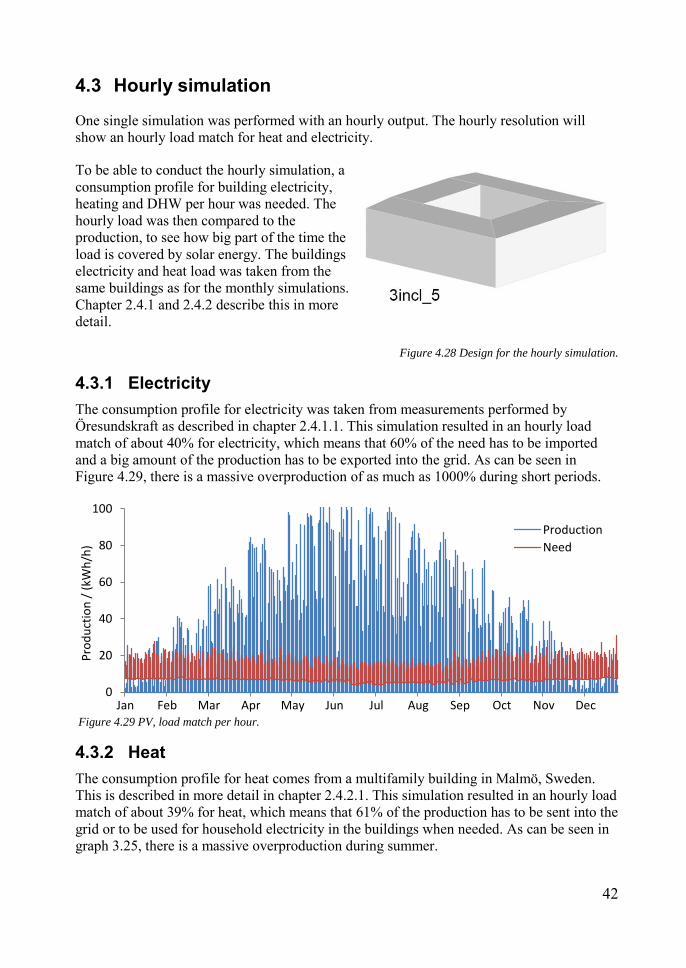
Figure 4.28 Design for the hourly simulation.

4.3.1 Electricity The consumption profile for electricity was taken from measurements performed by Öresundskraft as described in chapter 2.4.1.1. This simulation resulted in an hourly load match of about 40% for electricity, which means that 60% of the need has to be imported and a big amount of the production has to be exported into the grid. As can be seen in Figure 4.29, there is a massive overproduction of as much as 1000% during short periods.

Figure 4.29 PV, load match per hour.

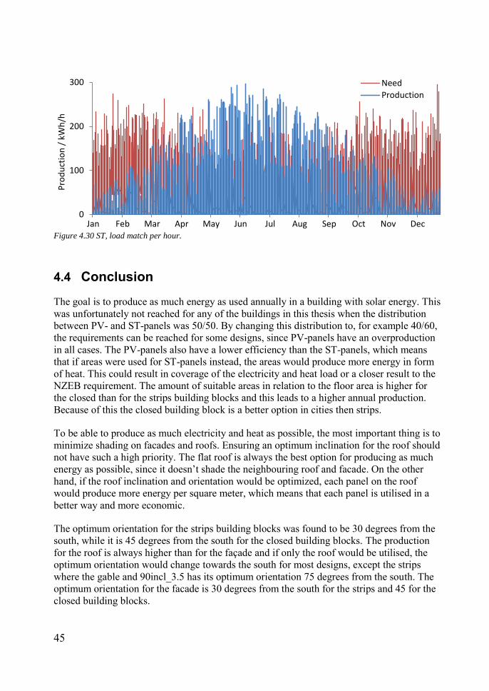
4.3.2 Heat The consumption profile for heat comes from a multifamily building in Malmö, Sweden. This is described in more detail in chapter 2.4.2.1. This simulation resulted in an hourly load match of about 39% for heat, which means that 61% of the production has to be sent into the grid or to be used for household electricity in the buildings when needed. As can be seen in graph 3.25, there is a massive overproduction during summer.

0

20

40

60

80

100


Pro

du

ctio

n /

(kW

h/h

)

Production

Need

45

Figure 4.30 ST, load match per hour.

4.4 Conclusion

The goal is to produce as much energy as used annually in a building with solar energy. This was unfortunately not reached for any of the buildings in this thesis when the distribution between PV- and ST-panels was 50/50. By changing this distribution to, for example 40/60, the requirements can be reached for some designs, since PV-panels have an overproduction in all cases. The PV-panels also have a lower efficiency than the ST-panels, which means that if areas were used for ST-panels instead, the areas would produce more energy in form of heat. This could result in coverage of the electricity and heat load or a closer result to the NZEB requirement. The amount of suitable areas in relation to the floor area is higher for the closed than for the strips building blocks and this leads to a higher annual production. Because of this the closed building block is a better option in cities then strips.

To be able to produce as much electricity and heat as possible, the most important thing is to minimize shading on facades and roofs. Ensuring an optimum inclination for the roof should not have such a high priority. The flat roof is always the best option for producing as much energy as possible, since it doesn’t shade the neighbouring roof and facade. On the other hand, if the roof inclination and orientation would be optimized, each panel on the roof would produce more energy per square meter, which means that each panel is utilised in a better way and more economic.

The optimum orientation for the strips building blocks was found to be 30 degrees from the south, while it is 45 degrees from the south for the closed building blocks. The production for the roof is always higher than for the façade and if only the roof would be utilised, the optimum orientation would change towards the south for most designs, except the strips where the gable and 90incl_3.5 has its optimum orientation 75 degrees from the south. The optimum orientation for the facade is 30 degrees from the south for the strips and 45 for the closed building blocks.

0

100

200

300


Pro

du

ctio

n /

kW

h/h

Need

Production

46

If only very well utilised areas should be used, the strips building block should be used, since this give a higher average irradiation on the roof than the closed building block. The buildings that have a high roof angle have the highest irradiation, but not the highest total production, since this will shade parts of the surrounding buildings. Strips_shed_incl_20 oriented towards the south is the building with the absolutely highest average irradiation. If the closed building block is used, it is instead the gable oriented 45 degrees from the south.

The six monthly simulations clearly show that the closed building block matches the load better than the strips per month. The reason to this might be that the closed building blocks have a higher annual energy production. The average of the load match per month for the PV-panels can reach a value of about 70% for the strips and 75% for the closed building blocks, while the ST-panels result is about 10% lower.

Matching the energy need in a building hourly with solar energy was proven to be impossible for some parts of the year due to the fact that peak production is at the wrong time. Peak production is in the middle of the day in the summer, while peak usage in residential buildings is in the morning, evening and winter when there is less or no solar irradiation at all. Despite this, the load match per hour was as high as 40% for electricity and 39% for heat.

4.4.1 Rules of thumb The most important factors for gaining solar energy are the orientation and choice of building block type. The roof design also has an impact, but not as big. A few roof designs should however be avoided, since they give a significantly lower production than others. For example, the buildings Closed_gable and Strips_90incl_3.5 have a significantly lower production for all orientations except 60 degrees from the south, when they give a comparable result to the other buildings.

An important issue is whether you should produce as much energy as possible or utilize only areas that have a very high irradiation. This issue can lead to two strategies:

47

Strategy one: Low buildings should be used.

To produce as much energy as possible, the roof area should be large in relation to the floor

area, since it often leads to a higher annual production. This means that lower buildings

produce more energy per square meter floor.

To produce as much energy as possible, all suitable areas should of course be utilized.

However, this does not always imply that the orientation should be towards the south. The

optimum orientation varies with the building type. For the two building types analysed in

this thesis, the best orientation was 45 (closed) and 30 (strips) degrees from the south.

A roof which does not shade the surrounding buildings is the best option to maximize the

production in cities. Therefore a flat roof or a roof with very low inclination towards the

south is always the best option. Inclinations towards the north should be avoided.

Strategy two: High inclined south facing roof.

If only areas with very high irradiation should be utilized, a high roof inclination oriented

towards the south should be used to maximize the irradiation per square meter. The

optimum orientation depends on the type of building block.

In this thesis, it is shown that the roofs of the strips building block have the absolutely

highest average irradiation when rotated towards the south.

If the closed building blocks are used, the optimum orientation for the roof is towards the

south as well, except for the gable roof where it is 45 degrees from the south. This will

however not give the highest total production, since the roof will shade surrounding

buildings, and especially the facades.

49

5 Economy in a solar energy system In this chapter, a lifecycle cost calculation (LCC) will be described to provide an understanding of how economically feasible a PV and ST system is in an urban environment. The limitations with life cycle cost calculations are that it is impossible to know how different parameters vary in the future.

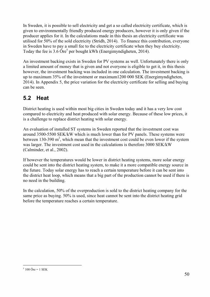
The LCC calculations were made for the building used in the hourly simulation. Closed_3incl_5 oriented 45 degrees from the south.

5.1 Electricity

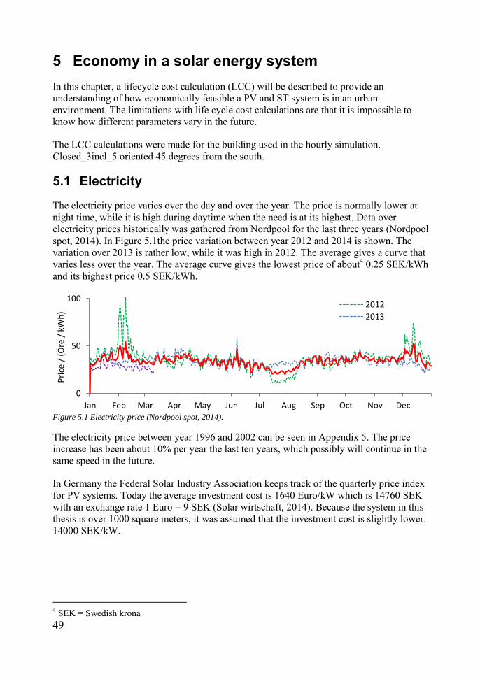
The electricity price varies over the day and over the year. The price is normally lower at night time, while it is high during daytime when the need is at its highest. Data over electricity prices historically was gathered from Nordpool for the last three years (Nordpool spot, 2014). In Figure 5.1the price variation between year 2012 and 2014 is shown. The variation over 2013 is rather low, while it was high in 2012. The average gives a curve that varies less over the year. The average curve gives the lowest price of about4 0.25 SEK/kWh and its highest price 0.5 SEK/kWh.

Figure 5.1 Electricity price (Nordpool spot, 2014).

The electricity price between year 1996 and 2002 can be seen in Appendix 5. The price increase has been about 10% per year the last ten years, which possibly will continue in the same speed in the future.

In Germany the Federal Solar Industry Association keeps track of the quarterly price index for PV systems. Today the average investment cost is 1640 Euro/kW which is 14760 SEK with an exchange rate 1 Euro = 9 SEK (Solar wirtschaft, 2014). Because the system in this thesis is over 1000 square meters, it was assumed that the investment cost is slightly lower. 14000 SEK/kW.

4 SEK = Swedish krona

0

50

100


Pri

ce /

(Ö

re /

kW

h)

2012

2013

50

In Sweden, it is possible to sell electricity and get a so called electricity certificate, which is given to environmentally friendly produced energy producers, however it is only given if the producer applies for it. In the calculations made in this thesis an electricity certificate was utilised for 50% of the sold electricity (Stridh, 2014). To finance this contribution, everyone in Sweden have to pay a small fee to the electricity certificate when they buy electricity. Today the fee is 3.6 Öre5 per bought kWh (Energimyndigheten, 2014).

An investment backing exists in Sweden for PV systems as well. Unfortunately there is only a limited amount of money that is given and not everyone is eligible to get it, in this thesis however, the investment backing was included in one calculation. The investment backing is up to maximum 35% of the investment or maximum1200 000 SEK (Energimyndigheten, 2014). In Appendix 5, the price variation for the electricity certificate for selling and buying can be seen.

5.2 Heat

District heating is used within most big cities in Sweden today and it has a very low cost compared to electricity and heat produced with solar energy. Because of these low prices, it is a challenge to replace district heating with solar energy.

An evaluation of installed ST systems in Sweden reported that the investment cost was around 3500-5500 SEK/kW which is much lower than for PV panels. These systems were between 130-390 m2, which mean that the investment cost could be even lower if the system was larger. The investment cost used in the calculations is therefore 3000 SEK/kW (Calminder, et al., 2002).

If however the temperatures would be lower in district heating systems, more solar energy could be sent into the district heating system, to make it a more compatible energy source in the future. Today solar energy has to reach a certain temperature before it can be sent into the district heat loop, which means that a big part of the production cannot be used if there is no need in the building.

In the calculation, 50% of the overproduction is sold to the district heating company for the same price as buying. 50% is used, since heat cannot be sent into the district heating grid before the temperature reaches a certain temperature.

5 100 Öre = 1 SEK

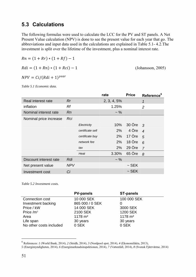
51

5.3 Calculations

The following formulas were used to calculate the LCC for the PV and ST panels. A Net Present Value calculation (NPV) is done to see the present value for each year that go. The abbreviations and input data used in the calculations are explained in Table 5.1- 4.2.The investment is split over the lifetime of the investment, plus a nominal interest rate.

( ) ( )

( ) ( ) (Johansson, 2005)

( )

Table 5.1 Economic data.

rate Price Reference6 Real interest rate Rr 2, 3, 4, 5% 1

inflation Rf 1.25% 2

Nominal interest rate Rn ~ %

Nominal price increase Rci

Electricity 10% 30 Öre 3

certificate sell 2% 4 Öre 4

certificate buy 2% 17 Öre 5

network fee 2% 18 Öre 6

tax 2% 29 Öre 7

Heat 3.30% 65 Öre 8

Discount interest rate Rdi ~ %

Net present value NPV ~ SEK

Investment cost Ci

~ SEK

Table 5.2 Investment costs.

6 References: 1 (World Bank, 2014), 2 (Stridh, 2014), 3 (Nordpool spot, 2014), 4 (Ekonomifakta, 2013), 5 (Energimyndigheten, 2014), 6 (Energimarknadsinspektionen, 2014), 7 (Vattenfall, 2014), 8 (Svensk Fjärrvärme, 2014)

PV-panels ST-panels Connection cost 10 000 SEK 100 000 SEK Investment backing 865 000 / 0 SEK 0 Price / kW 14 000 SEK 3000 SEK Price /m² 2100 SEK 1200 SEK Area 1178 m² 1178 m² Life span 30 years 30 years No other costs included 0 SEK 0 SEK

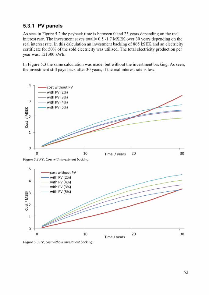
52

5.3.1 PV panels As sees in Figure 5.2 the payback time is between 0 and 23 years depending on the real interest rate. The investment saves totally 0.5 -1.7 MSEK over 30 years depending on the real interest rate. In this calculation an investment backing of 865 kSEK and an electricity certificate for 50% of the sold electricity was utilised. The total electricity production per year was: 121300 kWh.

In Figure 5.3 the same calculation was made, but without the investment backing. As seen, the investment still pays back after 30 years, if the real interest rate is low.

Figure 5.2 PV, Cost with investment backing.

Figure 5.3 PV, cost without investment backing.

0

1

2

3

4

0 10 20 30

Co

st /

MSE

K

Time / years

cost without PVwith PV (2%)with PV (3%)with PV (4%)with PV (5%)

0

1

2

3

4

5

0 10 20 30

Co

st /

MSE

K

Time / years

cost without PVwith PV (2%)with PV (4%)with PV (3%)with PV (5%)

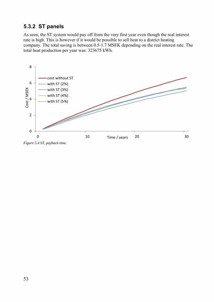
53

5.3.2 ST panels As seen, the ST system would pay off from the very first year even though the real interest rate is high. This is however if it would be possible to sell heat to a district heating company. The total saving is between 0.5-1.7 MSEK depending on the real interest rate. The total heat production per year was: 323675 kWh.

Figure 5.4 ST, payback time.

0

2

4

6

8

0 10 20 30

Co

st /

MSE

K

Time / years

cost without ST

with ST (2%)

with ST (3%)

with ST (4%)

with ST (5%)

55

6 Conclusion Solar energy should be used in urban areas, since plenty of suitable areas exist on buildings and it also appears to pay off economically. The question is if only areas that have very high irradiation should be utilised or if as much energy as possible should be produced.

The most important factors for gaining solar energy are the orientation and choice of building block type. The roof design also has an impact, but not as big.

To produce as much energy as possible annually, the roof area should be large in relation to the floor area. This means that lower buildings produce more energy per square meter floor. Still, this does not always imply that the orientation should be towards the south, since the optimum orientation varies with the building type.

The best roof design depends on if the building should produce as much energy as possible or only use areas that have a very high irradiation. If all suitable areas should be used for solar energy, the roof should have a low inclination closer to the south than the north, causing less shading on surrounding buildings. The highest irradiation is achieved on the roof and to achieve a very high irradiation, a roof with high inclination facing the south should be used. A few roof designs should however be avoided, since they give a significantly lower production than others. For example, the closed building with gable roof except when oriented 45 degrees from the south and the strips with a shed roof facing the east or west should be avoided. The roofs of the strokes building blocks achieve the absolutely highest irradiation of the two building blocks studied in this thesis.

A building with a high load match will also be more economical, since sold energy is not worth as much as the one used within the building. The monthly load match for the six different designs analysed only vary slightly, however there is a variation between the two different building blocks. The variation with different roof designs is almost not noticeable. When looking at an hourly resolution, the load match is about 40% for the example in this thesis, which mean that as much as 60% of the production has to be exported.

The most cost effective solution is possibly the building with very high irradiation available, since every square meter will produce more energy. Still the calculation made in this thesis apply that it is economically feasible to use all suitable areas, to produce as much energy as possible in most cases.

56

6.1 Continued work

This thesis was limited by a few factors, for example only two building block types were analysed, the orientation was only between 0-75 degrees from the north-south-axis, and only a few roof designs were tested.

A proposal of continued work is to make an analysis, which take into consideration PV panels’ sensitivity to shading, and how much it actually affects the output.

The integration of ST systems in the district heating system is another important factor. Since heat has to reach a certain temperature before being sent into the district heating grid, how much heat can actually be exported? A solution to this could be to use a heat pump driven by photovoltaic panels to increase the temperature when needed to the district heating companies’ limit.

57

7 References Andren, L., 2003. Solar installations: Practical Applications for the Built

Environment. 1st ed. s.l.:Routledge. Bellis, M., 2013. History: Photovoltaics Timeline. [Online] Available at: http://inventors.about.com/od/timelines/a/Photovoltaics.htm [Accessed 21 05 2014]. Ben, D., 2014. Solar Hot Warer. [Online] Available at: http://www.solarhotwater-systems.com/evacuated-tube-versus-flat-plate-solar-hot-water-panels/ [Accessed 21 05 2014]. Boverket, 2013. BBR20, s.l.: Boverket. Cakir, A. E., 2011. Daylight for Health and Efficiency - A new career for an old

friend. Berlin: Ergonomic Institut. Calminder, B., Landfors, K. & Södergren, L. O., 2002. Medelstora

solvärmeanläggningar, Stockholm: K-konsult Energi Stockholm AB. Dalenbäck, J. O., Lennermo, G., Andersson-Jenssen, P. E. & Kovacs, P., 2013. Solvärme i fjärrvärmesystem - Utverdering av primärkopplade system, s.l.: Svensk Fjärrvärme AB. Damon, 2014. Gallery.HD. [Online] Available at: http://gallery.hd.org/_tn/std/natural-science/_more2007/_more05/solar-cell-Si-silicon-monocrystalline-part-of-20W-17V-36-cell-panel-closeup-10-DHD.jpg [Accessed 21 05 2014]. Ekonomifakta, 2013. Elcertifikat. [Online] Available at: http://www.ekonomifakta.se/sv/Fakta/Energi/Styrmedel/Elcertifikat/ [Accessed 21 05 2014]. Energimarknadsinspektionen, 2014. Monopolföretagens årsrapporter och

nättariffer. [Online] Available at: http://www.inflation.eu/inflation-rates/sweden/historic-inflation/cpi-inflation-sweden.aspx [Accessed 21 05 2014]. Energimyndigheten, 2014. Elkundens kostnad. [Online] Available at: http://www.energimyndigheten.se/Foretag/Elcertifikat/elkundens_bidrag/ [Accessed 21 05 2014].

58

Energimyndigheten, 2014. Stöd för solceller. [Online] Available at: http://www.energimyndigheten.se/Hushall/Aktuella-bidrag-och-stod-du-kan-soka/Stod-till-solceller/ [Accessed 23 05 2014]. European Union, 2010. Directive 2010/31/EU of the European Parliament and of

the council of 19 May 2010 on the energy performance of buildings, s.l.: European parliament. Holsinger, J., 2014. Evaluate Solar Power. [Online] Available at: http://evaluatesolar.com/wp-content/uploads/2012/01/Polycrystalline-Silicon-Wafer.jpg[Accessed 21 05 2014]. Jakubiec, A. & Reinhart, F. C., 2011. DIVA 2.0: Integrating daylight and thermal simulations. Conference of International Building Performance Simulation

Association, pp. 2202-2209. Janson, U., 2010. Passive houses in Sweden - From design to evaluation of four

demonstration projects. Lund: Lunds University, LTH. Johansson, D., 2005. Modelling Life Cycle Cost for Indoor Climate Systems. Lund: Lunds University, LTH. Joint research center, 2009. PVGIS - interactive map. [Online] Available at: http://re.jrc.ec.europa.eu/pvgis/apps4/pvest.php#[Accessed 21 05 2014]. Joint Research Center, 2014. PVGIS. [Online] Available at: http://re.jrc.ec.europa.eu/pvgis/index.htm[Accessed 21 May 2014]. Kanters, J., 2014. Compare. [Online] Available at: http://www.solarplanning.org/compare.html [Accessed 21 05 2014]. Kanters, J., 2014. Solar planning. [Online] Available at: www.solarplanning.org [Accessed 21 05 2014].Kanters, J., 2014. Solar Planning Building blocks. [Online] Available at: http://www.solarplanning.org/assets/img/design.png [Accessed 21 05 2014]. Kanters, J., 2014. Solar Planning FSI. [Online] Available at: http://www.solarplanning.org/FSI.jpg [Accessed 21 05 2014]. Krishbaum, E., 2012. Germany sets new solar power record, institute says. [Online] Available at: http://www.reuters.com/article/2012/05/26/us-climate-germany-solar-idUSBRE84P0FI20120526 [Accessed 21 05 2014].

59

Lanardic, D., 2013. Shading Analysis in Photovoltaics. [Online] Available at: http://www.pvresources.com/siteanalysis/shading.aspx [Accessed 23 05 2014]. Martinez, A. R. L., 2014. Solar Thermal Energy History. [Online] Available at: http://www.solarthermalpowerplant.com/index.php/history-of-solar-thermal-energy [Accessed 21 05 2014]. Mr. Solar, 2010. Photovoltaic effect. [Online] Available at: http://www.mrsolar.com/content/photovoltaic-effect.php#.U33uTvmSySo [Accessed 21 05 2014]. Neij, L., Wall, M., Kjellsson, E. & Samuelsson, O., 2011. Solar energy in urban

planning. [Online] Available at: http://sustainability.formas.se/en/Issues/Issue-4-November-2011/Content/Focus-articles/Solar-energy-in-urban-planning/ [Accessed 21 05 2014]. Nordpool spot, 2014. Nordpool spot. [Online] Available at: http://www.nordpoolspot.com/[Accessed 21 05 2014]. NRDC, 2014. Global warming. [Online] Available at: http://www.nrdc.org/globalwarming/default.asp[Accessed 21 05 2014]. Pont, M. B. & Haupt, P., 2009. Space, Density and Urban Form. 1st ed. Delft: Technishe Universiteit Delft. Redweik, P., Catita, C. & Brito, M., 2013. Solar energy potential on roofs and facades in an urban landscape. Elsevier, Volume 97, pp. 332-341. Renewable energy hub, 2014. History behind solar thermal and solar water heating

technology. [Online] Available at: http://www.renewableenergyhub.co.uk/the-history-of-solar-thermal-technology.html [Accessed 21 05 2014]. Robert McNeel & Associates, 2014. Rhino3d. [Online] Available at: http://www.rhino3d.com/[Accessed 21 05 2014]. Satori, I., Napolitano, A. & Voss, K., 2012. Net zero energy buildings: A consistent definition framework. Elsevier, Volume 48, pp. 220-232. Sibbitt, B. et al., 2012. The performance of a High Solar Fraction Seasonal Storage District Heating System - Five Years of Operation. Elsevier, Volume 30, pp. 856-865.

60

Solar Tribune, 2014. Solar Tribune. [Online] Available at: http://solartribune.com/wp-content/uploads/2011/06/metaefficient.com-evacuated-tube-water-heater.jpg [Accessed 21 05 2014]. Solar wirtschaft, 2014. Price index photovoltaic. [Online] Available at: http://www.solarwirtschaft.de/preisindex [Accessed 23 05 2014]. Stridh, B., 2014. Produktionskostnad för solel i Sverige. [Online] Available at: http://bengts.blogg.viivilla.se/produktionskostnad-for-solel-i-sverige/ [Accessed 21 05 2014]. Stridh, B., 2014. Produktionskostnad för solel i Sverige. [Online] Available at: http://bengts.blogg.viivilla.se/produktionskostnad-for-solel-i-sverige/ [Accessed 23 05 2014]. Strømann-Andersen, J. & Sttrup, P. A., 2011. The urban canyon and building energy use: Urban desity versus daylight and passive solar gains. Elsevier, 43(8), pp. 2011-2020. SVEBY, 2009. Brukarindata för energiberäkningar i bostäder, Stockholm: SVEBY. Svensk Fjärrvärme, 2014. Fjärrvärmepriser. [Online] Available at: http://www.svenskfjarrvarme.se/Statistik--Pris/Fjarrvarmepriser/ [Accessed 21 05 2014]. Sveriges Centrum för Nollenergihus, 2012. Kravspecifikation för nollenergihus,

passivhus och minienergihus, FEBY12, s.l.: Sveriges Centrum för Nollenergihus. UK Solar Energy, 2014. UK Solar Energy. [Online] Available at: http://www.uksolarenergy.org.uk/images/fpc.jpg [Accessed 21 05 2014]. University of Central Florida, 2014. Types of PV Systems. [Online] Available at: http://www.fsec.ucf.edu/en/consumer/solar_electricity/basics/types_of_pv.htm [Accessed 21 05 2014]. Vattenfall, 2014. Energiskatter. [Online] Available at: http://www.vattenfall.se/sv/energiskatter.htm [Accessed 21 05 2014]. Wikipedia, 2006. Solar savings fraction. [Online] Available at: http://en.wikipedia.org/wiki/Solar_savings_fraction [Accessed 21 05 2014]. World Bank, 2014. Real interest rate. [Online] Available at: http://www.quandl.com/WORLDBANK/SWE_FR_INR_RINR-Sweden-Real-interest-rate [Accessed 21 05 2014].

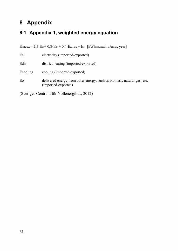
61

8 Appendix

8.1 Appendix 1, weighted energy equation

Ebalanced= 2,5·Eel + 0,8·Edh + 0,4·Ecooling + Eö [kWhbalanced/m2Atemp, year]

Eel electricity (imported-exported)

Edh district heating (imported-exported)

Ecooling cooling (imported-exported)

Eo delivered energy from other energy, such as biomass, natural gas, etc. (imported-exported)

(Sveriges Centrum för Nollenergihus, 2012)

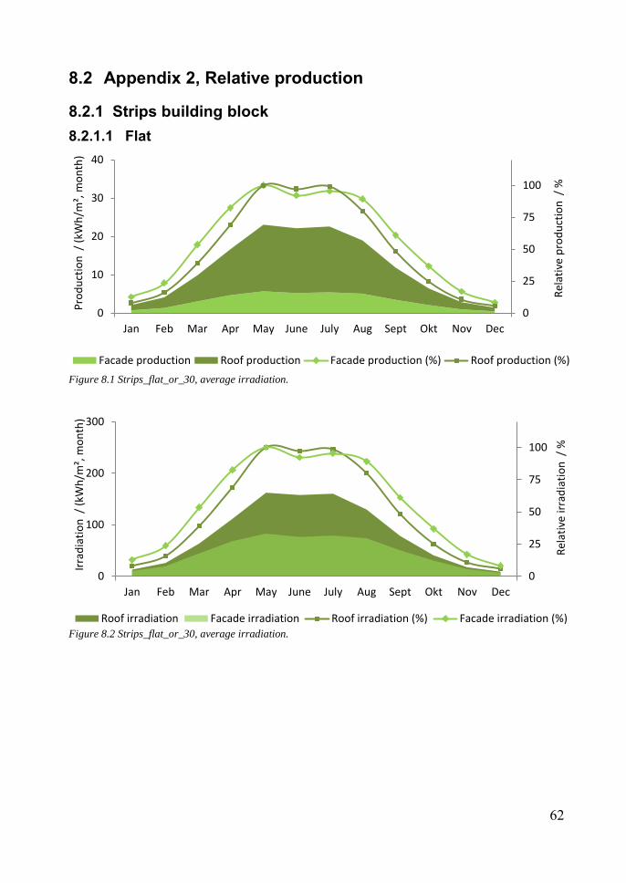
62

8.2 Appendix 2, Relative production

8.2.1 Strips building block 8.2.1.1 Flat

Figure 8.1 Strips_flat_or_30, average irradiation.

Figure 8.2 Strips_flat_or_30, average irradiation.

0

25

50

75

100

0

10

20

30

40


Rel

ativ

e p

rod

uct

ion

/ %

Pro

du

ctio

n /

(kW

h/m

², m

on

th)


0

25

50

75

100

0

100

200

300


Rel

ativ

e ir

rad

iati

on

/ %

Irra

dia

tio

n /

(kW

h/m

², m

on

th)


63

8.2.1.2 Shed_incl_10

Figure 8.3 Strips_shed_incl_10_or_30, production.

Figure 8.4 Strips_shed_incl_10_or_30, average irradiation.

0

25

50

75

100

0

10

20

30

40


Rel

ativ

e p

rod

uct

ion

/ %

Pro

du

ctio

n /

(kW

h/m

², m

on

th)


0

25

50

75

100

0

100

200

300


Rel

ativ

e ir

rad

iati

on

/ %

Irra

dia

tio

n /

(kW

h/m

², m

on

th)


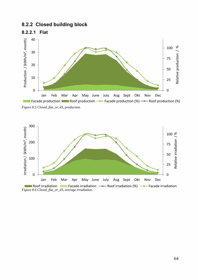
64

8.2.2 Closed building block 8.2.2.1 Flat

Figure 8.5 Closed_flat_or_45, production.

Figure 8.6 Closed_flat_or_45, average irradiation.

0

25

50

75

100

0

10

20

30

40


Rel

ativ

e p

rod

uct

ion

/ %

Pro

du

ctio

n /

(kW

h/m

², m

on

th)


0

25

50

75

100

0

100

200

300

Jan Feb Mar Apr May June July Aug Sept Okt Nov DecR

elat

ive

irra

dia

tio

n /

%

Irra

dia

tio

n /

(kW

h/m

², m

on

th)

Roof irradiation Facade irradiation Roof irradiation (%) Facade irradiation

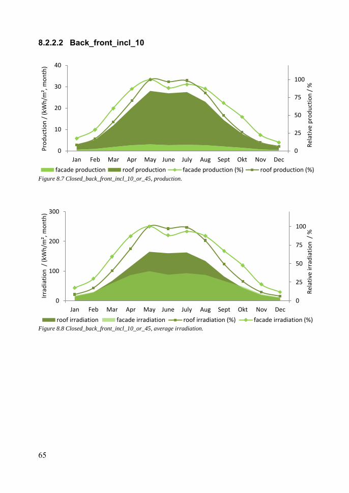
65

8.2.2.2 Back_front_incl_10

Figure 8.7 Closed_back_front_incl_10_or_45, production.

Figure 8.8 Closed_back_front_incl_10_or_45, average irradiation.

0

25

50

75

100

0

10

20

30

40


Rel

ativ

e p

rod

uct

ion

/ %

Pro

du

ctio

n /

(kW

h/m

², m

on

th)

facade production roof production facade production (%) roof production (%)

0

25

50

75

100

0

100

200

300

Jan Feb Mar Apr May June July Aug Sept Okt Nov DecR

elat

ive

irra

dia

tio

n /

%

Irra

dia

tio

n /

(kW

h/m

², m

on

th)

roof irradiation facade irradiation roof irradiation (%) facade irradiation (%)

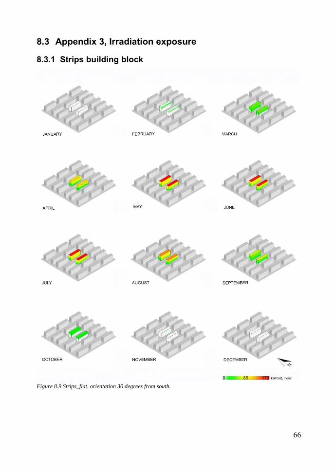
66

8.3 Appendix 3, Irradiation exposure

8.3.1 Strips building block

Figure 8.9 Strips_flat, orientation 30 degrees from south.

67

Figure 8.10 Strips_shed_incl_20, orientation 30 degrees from south.

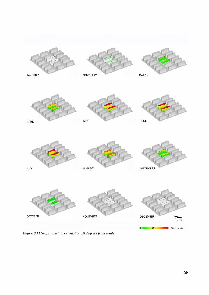
68

Figure 8.11 Strips_3incl_5, orientation 30 degrees from south.

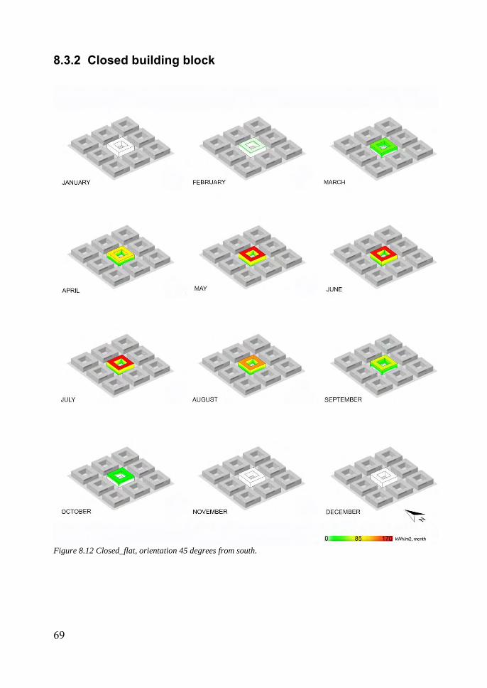
69

8.3.2 Closed building block

Figure 8.12 Closed_flat, orientation 45 degrees from south.

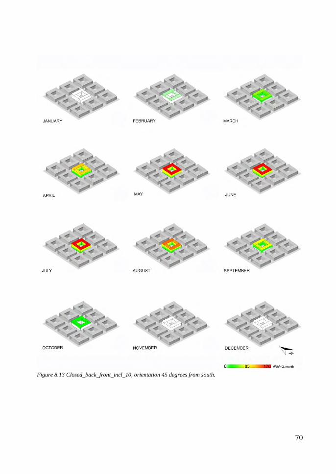
70

Figure 8.13 Closed_back_front_incl_10, orientation 45 degrees from south.

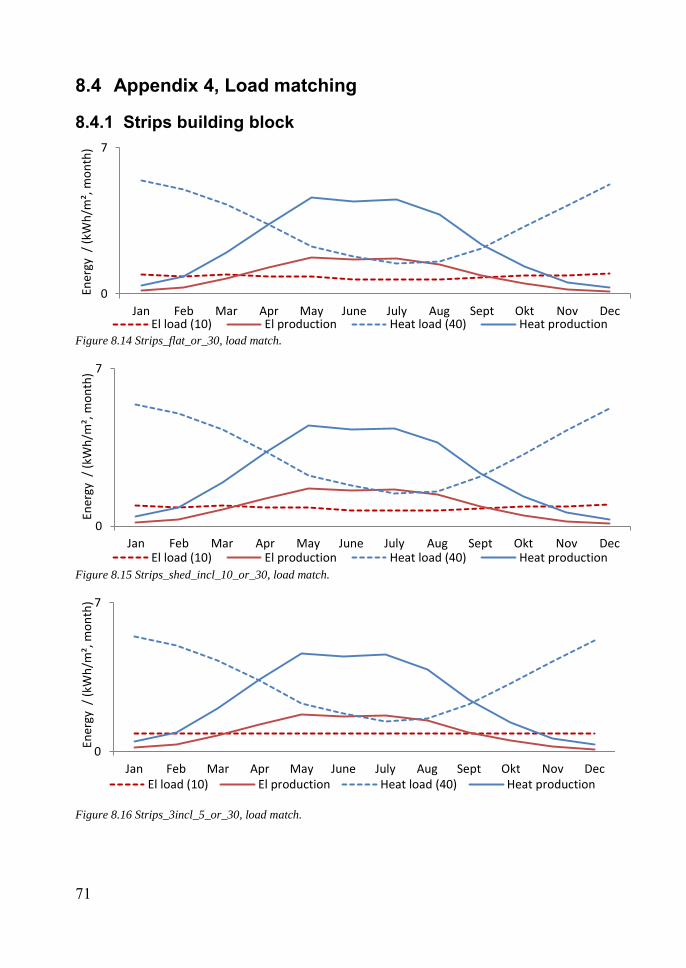
71

8.4 Appendix 4, Load matching

8.4.1 Strips building block

Figure 8.14 Strips_flat_or_30, load match.

Figure 8.15 Strips_shed_incl_10_or_30, load match.

Figure 8.16 Strips_3incl_5_or_30, load match.

0

7


Ener

gy /

(kW

h/m

², m

on

th)


0

7


Ener

gy /

(kW

h/m

², m

on

th)


0

7


Ener

gy /

(kW

h/m

², m

on

th)


72

8.4.2 Closed building block

Figure 8.17 Closed_flat_or_45, load match.

Figure 8.18 Closed_back_front_incl_10_or_45, load match.

0

7


Ener

gy /

(kW

h/m

², m

on

th)


0

7


Ener

gy /

(kW

h/m

², m

on

th)

el load (10) el production heat load (40) heat production

73

8.5 Appendix 5, LCC

8.5.1 Electricity price increase The electricity price has always increased, but especially much the last 15 years. The price increase has been about 17% per year since year 2000 when not taking the inflation into account in Sweden. The data is taken from Nordpol (Nordpool spot, 2014).

Figure 8.19 Electricity, price increase (Nordpool spot, 2014).

8.5.2 Electricity certificate price increase The average price of an electricity certificate is 222.8 Öre/kWh, and if a trend line is drawn, the trend says that the price will probably not rise or fall too much in the future, since the price has not varied that much since it was introduced in 2003. An electricity certificate is sold per MWh. The prices are taken from SKM (Svensk Kraftmärkning).

The amount that goes to the electricity certificate when buying electricity has increased about 25% per year if you look at the trend line. However, it decreased the last years.

Figure 8.20 Electricity certificate, price increase, sell (Ekonomifakta, 2013).

y = 0.17x

0

100

200

300

2000 2004 2008 2012

No

min

al p

rice

incr

ease

/%

0

20

40

2003 2005 2007 2009 2011 2013

Pri

ce (

Öre

/kW

h)

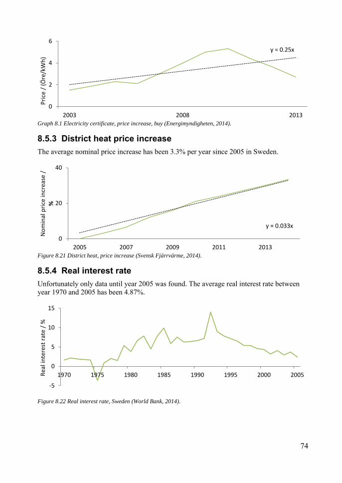
74

Graph 8.1 Electricity certificate, price increase, buy (Energimyndigheten, 2014).

8.5.3 District heat price increase The average nominal price increase has been 3.3% per year since 2005 in Sweden.

Figure 8.21 District heat, price increase (Svensk Fjärrvärme, 2014).

8.5.4 Real interest rate Unfortunately only data until year 2005 was found. The average real interest rate between year 1970 and 2005 has been 4.87%.

Figure 8.22 Real interest rate, Sweden (World Bank, 2014).

y = 0.25x

0

2

4

6

2003 2008 2013

Pri

ce /

(Ö

re/k

Wh

)

y = 0.033x

0

20

40

2005 2007 2009 2011 2013

No

min

al p

rice

incr

ease

/

%

-5

0

5

10

15

1970 1975 1980 1985 1990 1995 2000 2005Rea

l in

tere

st r

ate

/ %

Dept of Architecture and Built Environment: Division of Energy and Building DesignDept of Building and Environmental Technology: Divisions of Building Physics and Building Services

Lund University - Energy and Building Design | Energy and … · · 2016-05-02Lund University ....

Documents

Transcript of Lund University - Energy and Building Design | Energy and … · · 2016-05-02Lund University ....