LUIS GUIJARRO AND FREDERICK WILHELM … · Theorem B implies that the standard unit metric is the...

arX

iv:1

603.

0405

0v3

[m

ath.

DG

] 1

7 O

ct 2

017

FOCAL RADIUS, RIGIDITY, AND LOWER CURVATURE BOUNDS

LUIS GUIJARRO AND FREDERICK WILHELM

ABSTRACT. We prove a new comparison lemma for Jacobi fields that exploits Wilking’s trans-

verse Jacobi equation. In contrast to standard Riccati and Jacobi comparison theorems, there

are situations when our technique can be applied after the first conjugate point.

Using it we show that the focal radius of any submanifold N of positive dimension in a

manifold M with sectional curvature greater than or equal to 1 does not exceed π

2. In the case

of equality, we show that N is totally geodesic in M and the universal cover of M is isometric

to a sphere or a projective space with their standard metrics, provided N is closed.

Our results also hold for kth–intermediate Ricci curvature, provided the submanifold has

dimension ≥ k. Thus in a manifold with Ricci curvature ≥ n− 1, all hypersurfaces have focal

radius ≤ π

2, and space forms are the only such manifolds where equality can occur, if the

submanifold is closed.

Example 2.38 and Remark 3.4 show that our results cannot be proven using standard Riccati

or Jacobi comparison techniques.

A Riemannian manifold M has kth–intermediate Ricci curvature ≥ ℓ if for any orthonor-

mal (k + 1)–frame {v, w1, w2, . . . , wk} , the sectional curvature sum, Σki=1sec (v, wi) , is ≥ ℓ

([33], [27]). For brevity we write Rick M ≥ ℓ. Motivated by Myers theorem we show that if

Rick M ≥ k, then all submanifolds with dimension ≥ k have focal radius ≤ π2.

Theorem A. Let M be a complete Riemannian n–manifold with Rick ≥ k and N be any

submanifold of M with dim (N) ≥ k.

1. Every unit speed geodesic γ that leaves N orthogonally at time 0 has at least

dim (N) − k + 1 focal points for N in[−π

2, π2

], counting multiplicities. In particular, the

focal radius of N is ≤ π2.

2. If the focal radius of N is π2, then N is totally geodesic.

Since Ric1M ≥ ℓ means that all sectional curvatures of M are ≥ ℓ and Ricn−1M ≥ ℓmeans that M has Ricci curvature ≥ ℓ, the theorem applies to N ⊂ M if either the Ricci

curvature of M is ≥ n − 1 and N is a hypersurface, or the sectional curvature of M is ≥ 1and dim (N) ≥ 1.

We emphasize that N need not be closed or even complete, and there is no hypothesis about

its second fundamental form. On the other hand, if N happens to be closed and have focal

radius π2, then we determine M up to isometry.

Date: May 18, 2016.

2000 Mathematics Subject Classification. Primary 53C20.

Key words and phrases. Focal Radius, Rigidity, Projective Space, Positive Curvature.

The first author was supported by research grants MTM2011-22612, MTM2014-57769-3-P from the

MINECO, and by ICMAT Severo Ochoa project SEV-2015-0554 (MINECO).

This work was supported by a grant from the Simons Foundation (#358068, Frederick Wilhelm).

1

http://arxiv.org/abs/1603.04050v3

2 LUIS GUIJARRO AND FREDERICK WILHELM

Theorem B. Let M be a complete Riemannian n–manifold with Rick ≥ k. If M contains a

closed, embedded, submanifold N with focal radius π2

and dim (N) ≥ k, then N is totally

geodesic in M , and the universal cover of M is isometric to the sphere or a projective space

with the standard metrics.

In Section 3.1, we provide examples showing that the hypothesis on the dimension of Ncan not be dropped from either Theorem A or B.

In the course of proving Theorem B we will also establish the following corollary (see

Theorem 5.17, below.)

Corollary C. If the submanifold N of Theorem B is a hypersurface, then the universal cover

of M is isometric to the unit sphere.

It is reasonable to compare the Ricci curvature versions of Theorems A and B with the

Bonnet-Myers Theorem and Cheng’s Maximal Diameter Theorem (cf also Theorem 3 in [6]

and Theorem 1 in [10]). While an analogy can be made between the sectional curvature

version of Theorem B and the Diameter Rigidity Theorem ([14],[32]), the following example

shows that Theorem B applies to more nonsimply connected manifolds.

Example D. Let S3 be the unit sphere in C ⊕ C, and embed S1 as the unit circle in the first

copy of C. Let Q be the quaternion group of order 8 in SO (4) . Then the focal radius of

N = Q (S1) /Q in M = S3/Q is π2, and N is its own focal set. On the other hand, M has

diameter strictly smaller than π2.

More generally, let π : Sn −→ Sn/G be the quotient map of a properly discontinuous action

by G on Sn, and let N be any closed geodesic in Sn/G. Then π−1 (N) is the disjoint union of

closed geodesics in Sn, and hence both π−1 (N) and N have focal radius π2.

Theorem B implies that the standard unit metric is the only one on any topological sphere

with sectional curvature ≥ 1 that has a closed submanifold with focal radius π2. In contrast,

the conclusion of the Diameter Rigidity Theorem is softer, since there are many metrics on Sn

with curvature ≥ 1 and diameter ≥ π2, and there is even the possibility of such a metric on an

exotic sphere.

It is also reasonable to compare the sectional curvature version of Theorem B to the “rank

rigidity” results of Schmidt and Shankar–Spatzier–Wilking in [24] and [26]. Shankar, Spatzier,

and Wilking obtained the conclusion of Theorem B for manifolds with curvature less than or

equal to 1 and minimal conjugate radius π. Schmidt proves that if M has sectional curvature

≥ 1 and conjugate radius ≥ π2, then its universal cover is homeomorphic to Sn or isometric to

a projective space. The conjugate radius hypotheses of these theorems apply to every geodesic

in M. In contrast, the focal radius hypothesis of Theorem B only concerns the geodesics that

meet a single submanifold orthogonally.

To prove Theorems A and B, we exploit Wilking’s transverse Jacobi equation ([31]) to get

a new comparison lemma for Jacobi fields. To state it, we let γ : (−∞,∞) −→ M be a unit

speed geodesic in a complete Riemannian n–manifold M. We call an (n− 1)–dimensional

subspace Λ of normal Jacobi fields along γ, Lagrangian, if the restriction of the Riccati oper-

ator to Λ is self adjoint, that is, if

〈J1 (t) , J′

2 (t)〉 = 〈J ′

1 (t) , J2 (t)〉

FOCAL RADIUS, RIGIDITY, AND LOWER CURVATURE BOUNDS 3

for all t and for all J1, J2 ∈ Λ (see (1.2) below for the formal definition of the Riccati operator

on Λ).In Sections 1 and 2, we review Wilking’s transverse Jacobi equation, justify the name La-

grangian, and prove a comparison lemma for intermediate Ricci curvature. In the special

case when the sectional curvature is bounded from below our comparison result becomes the

following.

Lemma E. (Sectional Curvature Comparison) For κ = −1, 0, or 1, let γ : (−∞,∞) −→ Mbe a unit speed geodesic in a complete Riemannian n–manifold M with sec(γ, ·) ≥ κ. Let

J0 be a nonzero, normal Jacobi field along γ, and let Λ be a Lagrangian subspace of normal

Jacobi fields along γ with Riccati operator S such that J0 ∈ Λ.For t0 < tmax, suppose that Λ has no singularities on (t0, tmax) , and that λκ : [t0, tmax) −→

R is a solution of

λ′

κ + λ2κ + κ = 0 (1)

with

〈S (J0) , J0〉 |t0 ≤ λκ (t0) |J0 (t0)|2 . (2)

Then for each t1 ∈ [t0, tmax) there is a J1 ∈ Λ \ {0} so that

〈S (J1) , J1〉 |t1 ≤ λκ (t1) |J1 (t1)|2 . (3)

In particular, if κ = 1, α ∈ [0, π) , λ1 (t) = cot (t + α), and t0 ∈ [0, π − α) , then Λ has

a singularity by time π − α, that is, there is a J ∈ Λ \ {0} with J (t2) = 0 for some t2 ∈(t0, π − α] .

Lemma E holds in certain situations where Λ has singularities on [t0, tmax) , for example

when limt→t+0λκ (t) = ∞. We describe another such situation in Lemma 2.23, where the

reader will also find a discussion of the equality case.

The reader is probably familiar with the Riccati comparison theorem of Eschenburg-Heintze

in [9]. It requires the initial condition (2) to hold for all J0 ∈ Λ, while Lemma E only

demands that the initial condition holds for a single Jacobi field. This comes at the expense

that the derived future inequality (3) is only guaranteed to hold for a single Jacobi field, which

moreover, is not likely to be the original field. In Examples 2.37 and 2.38 (below), we show

that J1 can in fact be different from J0. A similar example can be found on page 463 of [18].

This phenomenon is tied to the nonvanishing of Wilking’s generalized A–tensor (see (1.8)).

The difference between Lemma E and the theorem of [9] is starker if one considers the

contrapositives: Lemma E implies that if Inequality (3) fails for all J1 ∈ Λ, then Inequality (2)

fails for all J ∈ Λ. In contrast, the theorem of [9] only gives that Inequality 2 fails for some

J ∈ Λ.The main tool to prove Theorem A is Lemma 2.23, which is a generalization of Lemma E

to intermediate Ricci curvature. So that we can prove Theorem B, Lemma 2.23 also includes

an analysis of the rigid situation. Other cases when rigidity occurs are given in Lemmas 2.26

and 2.27

The proof of Theorem B begins by establishing Proposition 4.4, which draws a strong anal-

ogy between N and one of the dual sets in the proof of the Diameter Rigidity Theorem. Exam-

ple D shows that we can only push this analogy so far. The dual sets of [14] are disjoint while


Example D shows that N can be its own focal set. In fact, one of the challenges of the proof of

Theorem B is showing that phenomena like Example D do not occur in the simply connected

case. In spite of the differences, our overall strategy is similar to that of [14], and our proof

employs ideas from there. To keep the exposition tight, we will often refrain from giving

further specific references to [14] and have made our exposition reasonably self-contained.

After the introduction, we establish notations and conventions. The remainder of the paper

is divided into two parts and eight sections. The sections are subordinate to the parts. Each

part and many of the sections begin with a detailed summary of the contents, so the outline

immediately below is only meant to indicate where each result is proven.

Part 1 contains Sections 1 to 3. In Section 1, we review Wilking’s transverse Jacobi equa-

tion; in Section 2 we state and prove Lemma 2.23, which is the main tool of the paper. Sub-

section 2.4 provides examples showing that J0 and J1 can indeed be different in Lemma E. In

Section 3, we prove Theorem A and give examples showing its optimality.

In Part 2, we prove Theorem B in Sections 4—8. In the special case of Theorem B, when

the sectional curvature is ≥ 1, the argument can be completed a little faster by an appeal to

the Diameter Rigidity Theorem. We do this in Section 7, and we complete the proof of the

general case of Theorem B in Section 8.

Remark F. The reader may have noticed that the hypotheses Rick ≥ k ·κ of Theorems A and

B are global, whereas in Lemma E, we only assumed that sec(γ, ·) ≥ κ.For the conclusion of Theorems A to hold, we in fact, only need Rick (γ, ·) ≥ k · κ for all

unit speed geodesics γ that leave N orthogonally at time zero. That is,

k∑

i=1

sec (γ, Ei) ≥ k · κ

for any orthonormal set {γ, E1, . . . , Ek} .On the other hand, our proof of Theorem B uses the global hypothesis Rick ≥ k ·κ and also

the fact that Lemma 2.23 and its rigidity case are valid with only the radial curvature lower

bound.

Acknowledgment. We are grateful to Karsten Grove and Curtis Pro for valuable critiques of

this manuscript. Special thanks go to Universidad Autonoma de Madrid for hosting a stay by

the second author during which this work was initiated.

NOTATIONS AND CONVENTIONS

Unless otherwise specified, all curves are parameterized at unit speed. Given v ∈ TM, we

denote the unique geodesic with γ′v (0) = v by γv.

Let N be a submanifold of the Riemannian manifold M. Let ν (N) be the normal bundle of

N ⊂ M. For every unit v ∈ ν (N) , there is a first time t1 ∈ (0,∞] at which γv (t1) is focal

for N along γv. We set

regN ≡ {tv ∈ ν (N) | |v| = 1 and t ∈ [0, t1)} .

We let g∗ be the metric on the domain regN obtained from pulling back (M, g) via the normal

exponential map. We use the term tangent focal point for a critical point of exp⊥N : ν (N) −→

M and the term focal point for a critical value of exp⊥N .


π : ν (N) −→ N will denote the projection of the normal bundle; N0 will be the 0–section

of ν (N) , and ν1 (N) will be the unit normal bundle of N. The fibers of ν (N) and ν1 (N)over x ∈ N will be called νx (N) and ν1

x (N).We let Λ be any Lagrangian family of normal Jacobi fields along a geodesic γ, and for any

subspace W ⊂ Λ we write

W (t) ≡ {J (t) | J ∈ W} ⊕ {J ′ (t) | J ∈ W and J (t) = 0} . (4)

When γ is a geodesic that leavesN orthogonally at time 0, we will write ΛN for the Lagrangian

family of normal Jacobi fields along γ corresponding to variations by geodesics that leave Northogonally at time 0. We call the elements of ΛN , N–Jacobi fields. According to Lemma

4.1 on page 227 of [7], ΛN consists of the following normal Jacobi fields J along γ:

ΛN ≡{J |J (0) = 0, J ′ (0) ∈ νγ(0) (N)

}⊕{J |J (0) ∈ Tγ(0)N and J ′ (0) = Sγ′(0)J (0)

},(5)

where Sγ′(0) is the shape operator of N determined by γ′ (0) , that is,

Sγ′(0) : Tγv(0)N −→ Tγv(0)N is

Sγ′(0) : w 7−→ (∇wγ′ (0))

TN.

We write Sn for the unit sphere in Rn+1, and for κ = −1, 0, or 1, we let S2κ be the simply

connected 2–dimensional space form of constant curvature κ.We use the acronym CROSS for Compact Rank One Symmetric Space. For convenience,

we normalize the nonspherical CROSSes so that their curvatures are in [1, 4] , and we normal-

ize the spherical CROSSes to have constant curvature 4.We write sec for sectional curvature and κ for our lower curvature bound. After rescaling,

we may always assume that κ is either −1, 0, or 1.Given r > 0 and A ⊂ M we set

B (A, r) ≡ {x ∈ M | dist (x,A) < r} ,

D (A, r) ≡ {x ∈ M | dist (x,A) ≤ r} , and

S (A, r) ≡ {x ∈ M | dist (x,A) = r} .

Finally, we write Dv (f) the derivative of f in the direction v.

Part 1: Bounding the Focal Radius

Part 1 is divided in three sections. Section 1 reviews Wilking’s transverse equation. In

Section 2, we state and prove Lemma 2.23, which is a generalization of Lemma E and is the

main tool of the paper; in subsection 2.4 we give an example that shows that J1 need not equal

J0 in Lemma E. Finally, in Section 3, we prove Theorem A, and give some examples showing

its optimality.

1. WILKING’S TRANSVERSE JACOBI EQUATION

In this section, we review Lagrangian families and Wilking’s transverse Jacobi equation.


1.1. Lagrangian Families. Let γ be a unit speed geodesic in a complete Riemannian n–

manifold M, and let J be the vector space of normal Jacobi fields along γ. Using symmetries

of the curvature tensor, we see that for J1, J2 ∈ J ,

ω (J1, J2) = 〈J ′

1, J2〉 − 〈J1, J′

2〉 ,

is constant along γ and hence defines a symplectic form on J .Thus an (n− 1)–dimensional subspace Λ of J on which ω vanishes is called Lagrangian.

Of course this is equivalent to saying that the restriction of the Riccati operator to Λ is self-

adjoint. Examples of Lagrangian families include the Jacobi fields that are 0 at time 0 and

those that correspond to variations by geodesics that leave a submanifold orthogonally at time

0.The set of times t so that

{J(t) | J ∈ Λ} = γ (t)⊥ (1.1)

is open and dense (cf Lemma 1.7 of [15]). For these t we get a well-defined Riccati operator

St : γ (t)⊥ −→ γ (t)⊥

St : v 7−→ J ′

v (t) , (1.2)

where Jv is the unique Jv ∈ Λ so that Jv (t) = v. The Jacobi equation then decomposes into

the two first order equations

St (J) = J ′, S ′

t + S2t +R = 0,

where S ′t is the covariant derivative of St along γ and R is the curvature along γ, that is

R (·) = R (·, γ) γ (see Equation 1.7.1 in [15]). We will omit the dependence on t if it is clear

from the context.

Remark 1.3. Given any W ⊂ Λ, and some t such that no Jacobi field in W \ {0} vanishes at

t, Equation (1.2) gives a well defined Riccati operator

St : W (t) −→ γ′ (t)⊥ .

This St agrees with the restriction of St defined in (1.2) when Λ has no zeros.

1.2. Singularities in the Lagrangian and the Riccati operator. The set of times t when

dim {J(t) | J ∈ Λ} < n− 1 (1.4)

corresponds to the moments where some of the Jacobi fields in Λ vanish. They are important

since, in general, they correspond to moments when the Riccati operator St is not defined.

Definition. Let V be a subspace of Λ. We will say that V has full index at t if any J ∈ Λ with

J(t) = 0 belongs to V; we will also say that V has full index on an interval I if it has full

index at each point of I .


There is a different way of stating the above condition: for fixed t ∈ R, define the evaluation

map as

Et : Λ −→ Tγ(t)M

Et : J 7−→ J (t) .

Observe that, for given t ∈ I , the kernel of Et is the set of those J ∈ Λ vanishing at t.Thus a subspace V ⊂ Λ has full index in an interval if and only if V contains the kernel of the

evaluation map Et for every t in the interval.

1.3. Wilking’s Transverse Jacobi Equation. Let V be any subspace of Λ. Set

V(t) ≡ {J(t) | J ∈ V} ⊕ {J ′(t) | J ∈ V, J(t) = 0}. (1.5)

Then V(t) is a smooth vector bundle along γ (Lemma 1.7.1 in [15], or [31]). Set

H(t) ≡ V(t)⊥ ∩ γ(t)⊥.

Proposition 1.6. Fix t ∈ I and suppose that V has full index at t.

1. For x ∈ H (t) , there is a J ∈ Λ so that J (t) = x.

2. We have a well-defined Riccati operator

St : H (t) −→ H (t)

given by

St (x) = J ′H (t) , (1.7)

where J is an element of Λ so that J (t) = x, and J ′H (t) is the H (t)–component of J ′ (t); in

other words, St is the H(t)-projection of St|H(t).

Proof. Since Λ is Lagrangian, the splitting

Λ (t) = {J(t) | J ∈ Λ} ⊕ {J ′(t) | J ∈ Λ, J(t) = 0}

is orthogonal. Since the kernel of Et lies in V, H (t) is contained in the first summand, and

Part 1 follows.

For the second part, suppose x = J1 (t) = J2 (t) ∈ H (t) and J1, J2 ∈ Λ. Since J1 − J2

vanishes at t and Kernel (Et) ⊂ V, we have J1 − J2 ∈ V. Together with (J1 − J2) (t) = 0,

this implies that (J1 − J2)′ (t) ∈ V(t). Thus

((J1 − J2)

′ (t))H

= 0, and S(x) is independent

of the choice of J ∈ Λ so that J(t) = x. �

We will call S the Riccati operator associated to V , if it is clear which Lagrangian Λ is

being used.

Wilking also defined maps

At : V (t) −→ H (t) given by,

At (v) = (J ′)h(t) , where J ∈ V, J (t) = v. (1.8)


A priori, At is only defined at points where Λ has no zeros; however, A extends smoothly

to R (cf. [31]). Indeed, let A∗t : H (t) −→ V (t) be the adjoint of At, and let X be a field in H

so that (X ′)H ≡ 0. According to Equation 1.7.6 on page 38 of [15],

X ′ = −A∗X.

Since the left-hand side is smooth, A∗ is smooth, and it follows that A is smooth.

Theorem 1.9 (Wilking [31]). S is self-adjoint, and

S ′ + S2 + {R (·, γ) γ}h + 3AA∗ = 0. (1.10)

Equation (1.10) is known as the Transverse Jacobi Equation. It is a vast generalization of

the Horizontal Curvature Equation of [12] and [21]. For details see [16] or [19].

Proposition 1.6 only gives us that S is defined almost everywhere. However, S ′ + S2 has a

smooth extension to all of R, because {R (·, γ) γ}h + 3AA∗ is smooth everywhere (see [31]

for an interpretation of S ′ + S2 as a second order differential operator H (t) −→ H (t)).

1.4. Splitting of Lagrangians. Like the Gray-O’Neill A–tensor, the Wilking A–tensor van-

ishes identically along a geodesic γ if and only if the distributions V (t) and H (t) are parallel

along γ. In this case, it follows that the subspaces of Λ,

{J ∈ Λ | J (t) ∈ H (t)} ,

are independent of t, and the parallel, orthogonal splitting V (t) ⊕ H (t) is given by Jacobi

fields. We make this more rigorous in what follows.

Lemma 1.11. With the above notation, assume that At = 0 for every t ∈ I . Then

1. V(t) and H(t) are parallel distributions along γ.

2. If for some t ∈ I , a Jacobi field J ∈ Λ has J(t) ∈ H(t), then J(t) ∈ H(t) for every t.3. There is a subspace H ⊂ Λ such that H(t) = H(t) for every t.

Proof. By continuity, it is enough to check the first part at times t ∈ I where Λ has no zeros.

Since any section of the bundle V(t) can be written as

Y =∑

i

fi · Ji,

where Ji are a basis of V , we have that

Y ′H =∑

i

fi · J′Hi = 0

since At ≡ 0. Therefore V(t), and consequently V⊥ = H, are both parallel, proving the first

part of the Lemma.

Since V(t) is parallel and spanned by Jacobi fields, it follows that R (·, γ′) γ′ leaves V(t)invariant. From this it follows that R (·, γ′) γ′ leaves H(t) invariant. Combining this with the

fact that H(t) is parallel, we get Part 2.

For the last part, choose a set {J1, . . . Jℓ} in Λ such that for some t ∈ I , {J1(t), . . . Jℓ(t)}is a basis of H(t). As previously shown, {J1(t), . . . Jℓ(t)} are in H(t) for any t ∈ I , and it is

a basis of H(t) whenever Λ has no zeros at that t. By continuity, the subspace H spanned by

{J1, . . . Jℓ} satisfies the third part of the Lemma. �


2. COMPARISON THEORY FOR THE TRANSVERSE JACOBI EQUATION

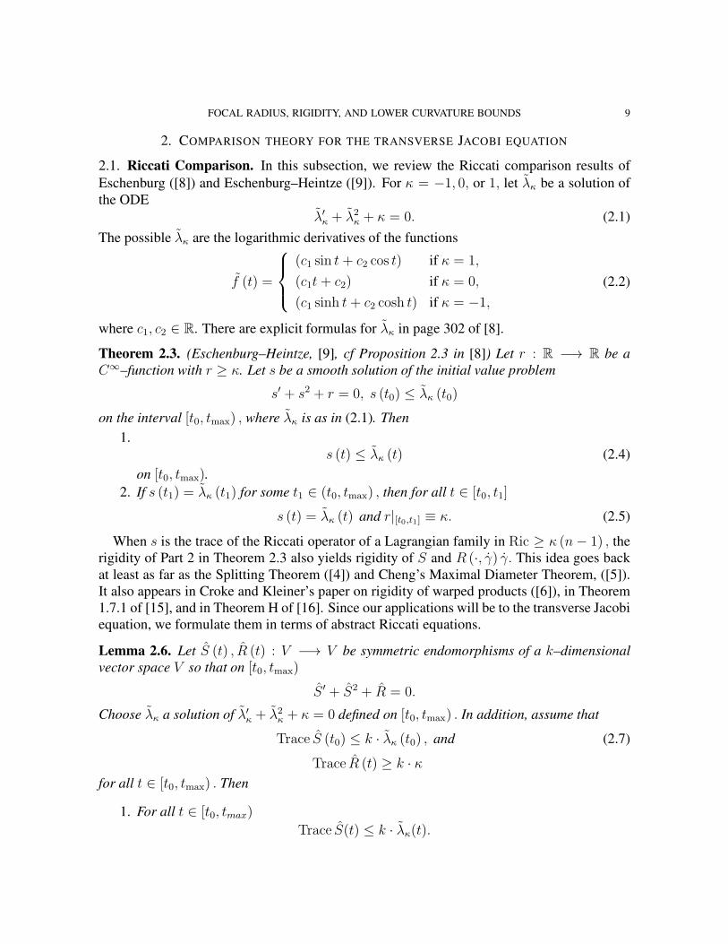
2.1. Riccati Comparison. In this subsection, we review the Riccati comparison results of

Eschenburg ([8]) and Eschenburg–Heintze ([9]). For κ = −1, 0, or 1, let λκ be a solution of

the ODE

λ′

κ + λ2κ + κ = 0. (2.1)

The possible λκ are the logarithmic derivatives of the functions

f (t) =

(c1 sin t + c2 cos t) if κ = 1,

(c1t + c2) if κ = 0,

(c1 sinh t+ c2 cosh t) if κ = −1,

(2.2)

where c1, c2 ∈ R. There are explicit formulas for λκ in page 302 of [8].

Theorem 2.3. (Eschenburg–Heintze, [9], cf Proposition 2.3 in [8]) Let r : R −→ R be a

C∞–function with r ≥ κ. Let s be a smooth solution of the initial value problem

s′ + s2 + r = 0, s (t0) ≤ λκ (t0)

on the interval [t0, tmax) , where λκ is as in (2.1). Then

1.

s (t) ≤ λκ (t) (2.4)

on [t0, tmax).

2. If s (t1) = λκ (t1) for some t1 ∈ (t0, tmax) , then for all t ∈ [t0, t1]

s (t) = λκ (t) and r|[t0,t1] ≡ κ. (2.5)

When s is the trace of the Riccati operator of a Lagrangian family in Ric ≥ κ (n− 1) , the

rigidity of Part 2 in Theorem 2.3 also yields rigidity of S and R (·, γ) γ. This idea goes back

at least as far as the Splitting Theorem ([4]) and Cheng’s Maximal Diameter Theorem, ([5]).

It also appears in Croke and Kleiner’s paper on rigidity of warped products ([6]), in Theorem

1.7.1 of [15], and in Theorem H of [16]. Since our applications will be to the transverse Jacobi

equation, we formulate them in terms of abstract Riccati equations.

Lemma 2.6. Let S (t) , R (t) : V −→ V be symmetric endomorphisms of a k–dimensional

vector space V so that on [t0, tmax)

S ′ + S2 + R = 0.

Choose λκ a solution of λ′κ + λ2

κ + κ = 0 defined on [t0, tmax) . In addition, assume that

Trace S (t0) ≤ k · λκ (t0) , and (2.7)

Trace R (t) ≥ k · κ

for all t ∈ [t0, tmax) . Then

1. For all t ∈ [t0, tmax)

Trace S(t) ≤ k · λκ(t).


2. If Trace S (t1) = kλκ (t1) for some t1 ∈ (t0, tmax] , then

S ≡ λκ · id and R = κ · id (2.8)

on [t0, t1], and the solutions of the Jacobi equation J ′′ + RJ = 0 on [t0, t1], have the

form

J(t) = f(t) · E, (2.9)

where E is a constant vector in V and f is the function from (2.2) that satisfies f (t0) =|J (t0)| .

Proof. Set

s ≡1

kTrace S,

S0 ≡ S −Trace S

k· id, and (2.10)

r ≡1

k

(Trace R +

∣∣∣S0

∣∣∣2).

Taking the trace of

S ′ + S2 + R = 0

yields

s′ + s2 + r = 0.

From inequalities (2.4) and (2.7), we get that

s (t) ≤ λκ (t) (2.11)

for all t ∈ (t0, tmax), and the first part follows.

For the second part, if Trace S (t1) = kλκ (t1) for some t1 ∈ (t0, tmax] , then Equation (2.5)

gives us s(t) ≡ λκ (t) and r ≡ κ in the subinterval [t0, t1].Consequently,

κ = r =Trace R + |S0|

2

k≥

κk + |S0|2

k= κ+

|S0|2

k.

Thus |S0| ≡ 0 and

S =Trace S

k· id = s · id = λκ (t) · id .

Substituting S = λκ (t) · id into the Riccati equation, S2 + S ′ + R = 0, gives

(λ2κ + λ′

κ) · id+R = 0,

−κ · id+R = 0, and

R = κ · id .

So the Jacobi fields have the form in equation (2.9). �

Remark 2.12. When κ = 0 and tmax = ∞, the above Lemma states that if Trace S(t0) ≤ 0,

then Trace S(t) ≤ 0 for any t ≥ t0, since in this case, λ0 ≡ 0 satisfies condition (2.7). The

following result improves this observation.


Lemma 2.13 (Long geodesics in nonnegative curvature). For S and R as in Lemma 2.6,

suppose that

Trace S (t0) ≤ 0, and Trace R (t) ≥ 0 (2.14)

for all t ∈ [t0,∞). If S is defined on [t0,∞), then

S ≡ 0 and R = 0, (2.15)

on [t0,∞) .

Proof. As in the previous proof, (2.4) gives

s (t) ≤ 0 (2.16)

for all t ∈ [t0,∞) . If for some t1 > t0, s(t1) < 0, then there is some c > t1 such that

s(t1) =1

t1 − c.

Thus, for

λ0(t) =1

t− c,

we get from (2.4) that

s(t) ≤ λ0(t)

for all t ∈ [t1, c), and in particular, s(t) could not be defined after c. Since this contradicts our

hypothesis on S being defined on [t0,∞), we obtain that s ≡ 0 and r ≡ 0 for all t ∈ (t0,∞) .The rest of the proof follows as in Lemma 2.6. �

For arbitrary curvature, there is also a rigidity statement:

Lemma 2.17. Let λκ be as in (2.1), and have no singularities on (t0, tmax). Suppose that

Trace S (t0) ≤ k · λκ (t0) , and Trace R (t) ≥ k · κ (2.18)

for all t ∈ [t0, tmax) . If S is defined on [t0,∞) and

limt→t−max

λκ (t) = −∞,

then

S ≡ λκ · id and R = κ · id (2.19)

holds on [t0, tmax) .

Proof. The hypothesis limt→t−maxλκ (t) = −∞ implies that

λκ (t) =

cot (π + t− tmax) if κ = 1,1

t−tmaxif κ = 0,

coth (t− tmax) if κ = −1

(see, e.g., page 302 of [8]). Since λκ has no singularities on (t0, tmax) , it follows that λκ (t) is

strictly decreasing on (t0, tmax) . So if s(t1) < λκ(t1) for some t1 ∈ (t0, tmax), then there is an

α ∈ (0, tmax − t1) so that

s (t1) ≤ λκ (t1 + α) .


Thus by (2.4),

s (t) ≤ λκ (t + α)

for all t ∈ (t1, tmax) . In particular, for some tmax ∈ (t0, tmax − α] , limt→t−maxs (t) = −∞.

Since this contradicts our hypothesis that S is defined on (t0, tmax) , Inequality (2.11) must be

an equality for all t ∈ (t0, tmax) and r ≡ κ. �

Remark 2.20. In the event that limt→t+0λκ (t) = ∞, Theorem 2.3 and Lemmas 2.6, 2.13, and

2.17, hold with the hypothesis s (t0) =1kTrace S ≤ λκ (t0) replaced by

limt→t+0

inf(λκ (t)− s (t)

)≥ 0. (2.21)

If s is the trace of the Riccati operator of the Lagrangian family {J | J (t0) = 0} along a

geodesic in a Riemannian manifold, then Inequality (2.21) is satisfied with

λκ (t) =

cot(t− t0) if κ = 11

t−t0if κ = 0

coth(t− t0) if κ = −1

(see Theorem 27 on page 175 of [23]). So, for example, in this case, Theorem 2.3 implies the

classical Rauch Comparison Theorem for 2–manifolds.

2.2. Statements of Comparison Lemmas. For a subspace W ⊂ Λ, write

W (t) = {J (t) | J ∈ W} ⊕ {J ′ (t) | J ∈ W and J (t) = 0} ,

and

PW ,t : Λ (t) −→ W (t)

for orthogonal projection. For simplicity of notation we will write

TraceSt|W for Trace(PW ,t ◦ St|W(t)

).

Remark 2.22. Choose a fixed t0 ∈ R; given any subspace Wt0 ⊥ γ′(t0), Wt0 becomes the

horizontal subspace H(t0) for Wilking’s equation when we choose V as the subset of Λ formed

by Jacobi fields J with J(t0) ⊥ Wt0 .

By considering 1–dimensional subspaces, we see that Lemma E is a special case of the fol-

lowing result. In its statement we write Rick (γ, ·) ≥ k · κ to mean that the radial intermediate

Ricci curvatures along γ are bounded from below by k · κ, that is,

k∑

i=1

sec (γ, Ei) ≥ k · κ

for any orthonormal set {γ, E1, . . . , Ek} .

Lemma 2.23 (Intermediate Ricci Comparison). For κ = −1, 0, or 1, let γ : (−∞,∞) −→ Mbe a unit speed geodesic in a complete Riemannian n–manifold M with Rick (γ, ·) ≥ k · κ.Let Λ be a Lagrangian subspace of normal Jacobi fields along γ with Riccati operator S, and

let Wt0 ⊥ γ′(t0) be some k–dimensional subspace such that

Trace(St0)|Wt0≤ k · λκ (t0) , (2.24)


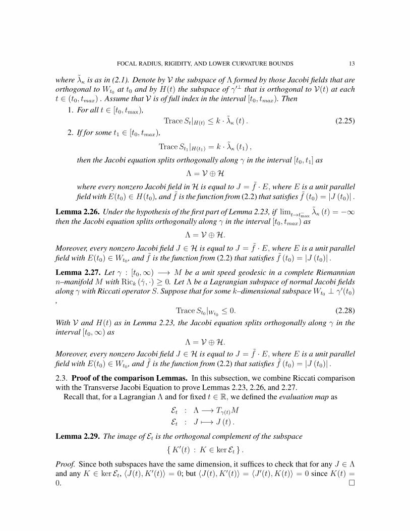
where λκ is as in (2.1). Denote by V the subspace of Λ formed by those Jacobi fields that are

orthogonal to Wt0 at t0 and by H(t) the subspace of γ′⊥ that is orthogonal to V(t) at each

t ∈ (t0, tmax) . Assume that V is of full index in the interval [t0, tmax). Then

1. For all t ∈ [t0, tmax),

TraceSt|H(t) ≤ k · λκ (t) . (2.25)

2. If for some t1 ∈ [t0, tmax),

TraceSt1 |H(t1) = k · λκ (t1) ,

then the Jacobi equation splits orthogonally along γ in the interval [t0, t1] as

Λ = V ⊕H

where every nonzero Jacobi field in H is equal to J = f ·E, where E is a unit parallel

field with E(t0) ∈ H(t0), and f is the function from (2.2) that satisfies f (t0) = |J (t0)| .

Lemma 2.26. Under the hypothesis of the first part of Lemma 2.23, if limt→t−maxλκ (t) = −∞

then the Jacobi equation splits orthogonally along γ in the interval [t0, tmax) as

Λ = V ⊕H.

Moreover, every nonzero Jacobi field J ∈ H is equal to J = f · E, where E is a unit parallel

field with E(t0) ∈ Wt0 , and f is the function from (2.2) that satisfies f (t0) = |J (t0)| .

Lemma 2.27. Let γ : [t0,∞) −→ M be a unit speed geodesic in a complete Riemannian

n–manifold M with Rick (γ, ·) ≥ 0. Let Λ be a Lagrangian subspace of normal Jacobi fields

along γ with Riccati operator S. Suppose that for some k–dimensional subspace Wt0 ⊥ γ′(t0),

TraceSt0 |Wt0≤ 0. (2.28)

With V and H(t) as in Lemma 2.23, the Jacobi equation splits orthogonally along γ in the

interval [t0,∞) as

Λ = V ⊕H.

Moreover, every nonzero Jacobi field J ∈ H is equal to J = f · E, where E is a unit parallel

field with E(t0) ∈ Wt0 , and f is the function from (2.2) that satisfies f (t0) = |J (t0)| .

2.3. Proof of the comparison Lemmas. In this subsection, we combine Riccati comparison

with the Transverse Jacobi Equation to prove Lemmas 2.23, 2.26, and 2.27.

Recall that, for a Lagrangian Λ and for fixed t ∈ R, we defined the evaluation map as

Et : Λ −→ Tγ(t)M

Et : J 7−→ J (t) .

Lemma 2.29. The image of Et is the orthogonal complement of the subspace

{K ′(t) : K ∈ ker Et } .

Proof. Since both subspaces have the same dimension, it suffices to check that for any J ∈ Λand any K ∈ ker Et, 〈J(t), K

′(t)〉 = 0; but 〈J(t), K ′(t)〉 = 〈J ′(t), K(t)〉 = 0 since K(t) =0. �


Lemma 2.30. (Eigenvalue Transfer Lemma) Let γ : [0, l] −→ M and Λ be as in Lemma 2.23.

Let V be an (n− 1− k)–dimensional subspace of Λ with full index in [0, l]. For any subspace

W of Λ, define W (t) as in (4).

1. For each fixed t ∈ [0, l] , there is a k–dimensional subspace W of Λ so that W (t) is the

orthogonal complement of V (t) . If Et is one-to-one, then W is unique.

2. Let St : H(t) → H(t) be the Riccati operator defined in (1.7). Then for any W as in

Part 1,

Trace St = TraceSt|W .

where TraceSt|W = Trace(PW ,t ◦ St|W(t)

), and PW ,t : Λ (t) −→ W (t) is orthogonal

projection.

Remark 2.31. For any W as in Part 1, St|W is well defined via Remark 1.3.

Proof. Since ker Et ⊂ V , we have that

{ J ′(t) : J ∈ ker Et } ⊂ V(t),

and by Lemma 2.29,

V(t)⊥ ⊂ image Et.

Thus there exist some k-dimensional subspace W ⊂ Λ with W(t) = V(t)⊥, and if Et is

one-to-one, then it is an isomorphism onto V (t)⊥ , so W is unique.

To prove Part 2, for J ∈ W, we write

J⊥ = J − JV ,

where JV is the component of J that lies in V (t) . Then for all t,

0 =d

dt

⟨JV , J⊥

⟩=

⟨(JV

)′, J⊥

⟩+⟨JV , J⊥′

⟩.

Since J ∈ W, JV (t) = 0, and⟨JV , J⊥′

⟩|t = 0. So the previous display evaluated at t

becomes ⟨(JV

)′, J⊥

⟩∣∣∣t= 0.

For J ∈ W, it follows that⟨S(J⊥

), J⊥

⟩∣∣∣t

=⟨(

J ′ −(JV

)′), J⊥

⟩∣∣∣t

=⟨J ′, J⊥

⟩∣∣t

=⟨S (J) , J⊥

⟩∣∣t

= 〈S (J) , J〉|t . (2.32)

So

Trace St = TraceSt|W(t).

�


Proof of Lemma 2.23. We combine Theorem 2.3 and Lemma 2.6 with the Transverse Jacobi

Equation, and the Eigenvalue Transfer Lemma 2.30.

Observe first that Theorem 2.3 holds on intervals where the function s is smooth. In our

context, this happens as long as S is well-defined. According to Proposition 1.6, S is well-

defined at all times t where V has full index at t, and therefore we can apply it in the situation

of Lemma 2.23.

Recall that

V ≡ {X ∈ Λ | X (t0) ⊥ J (t0) for all J ∈ Wt0} .

Let S : H (t) −→ H (t) be as in Equation (1.7). It follows from the Eigenvalue Transfer

Lemma 2.30 that

Trace St0 ≤ k · λκ (t0) .

The Transverse Jacobi Equation says,

S ′ + S2 + {R (·, γ(t)) γ(t)}h + 3AA∗ = 0. (2.33)

Since Rick ≥ k, AA∗ is nonnegative, and Wt0 is k–dimensional, when we take the trace

of Equation (2.33), divide by k, and make the substitutions of (2.10), we get an equation that

satisfies the hypotheses of Theorem 2.3. Thus for all t ∈ [t0, tmax) ,

1

kTrace St ≤ λκ (t) . (2.34)

By combining this with the Eigenvalue Transfer Lemma 2.30 and the fact that V has full

index on (t0, tmax) , we have

TraceS|H(t) ≤ k · λκ,

as claimed.

To prove the rigidity statement, suppose that

TraceS|H(t1) = k · λκ (t1)

for some t1 ∈ (t0, tmax) .It follows from Lemma 2.30 that

Trace St1 = k · λκ (t1) .

Writing R for {R (·, γ(t)) γ(t)}h + 3AA∗, we see from Theorem 2.3 that

Trace St ≡ k · λκ (t) and Trace R ≡ k · κ

for all t ∈ [t0, t1] .

Our hypothesis that Rick ≥ k · κ implies that Trace {R (·, γ(t)) γ(t)}h ≥ k · κ. Combining

this with Trace R ≡ k · κ and the fact that AA∗ is nonnegative, we see that A ≡ 0. So Lemma

1.11 guarantees the existence of a subspace H in Λ such that H(t) = H(t) at every t ∈ [t0, t1],and Λ splits orthogonally as

Λ = V ⊕H.

By Part 2 of Lemma 2.6, S ≡ λκ · id and R = κ · id. So it follows that H consists of Jacobi

fields whose restrictions to [t0, t1] have the form

J = fE,


where E is a parallel field and f is the function from (2.2) that satisfies f (t0) = |J (t0)| . �

Proof of Lemma 2.26. Since V has full index, Proposition 1.6 implies that S is defined on

[t0, tmax). As above, the Eigenvalue Transfer Lemma 2.30 gives us that

Trace St0 ≤ k · λκ (t0) .

Once again, Rick ≥ k · κ implies that Trace {R (·, γ(t)) γ(t)}h ≥ k · κ and R ≥ k · κ. So

by Lemma 2.17, S ≡ λκ · id and R = κ · id on [t0, tmax). This implies, as in the proof of Part

2 of Lemma 2.23, that A = 0 in [t0, tmax). The remainder of the argument is exactly the same

as the proof of Part 2 of Lemma 2.23. �

Proof of Lemma 2.27. Since V has full index, Proposition 1.6 gives that S is defined on [t0,∞) .As above, the Eigenvalue Transfer Lemma 2.30 gives us that

Trace St0 ≤ 0.

So by Lemma 2.13, S ≡ 0 and R ≡ 0 on [t0,∞) . As before, our hypothesis that Rick ≥ 0

implies that Trace {R (·, γ(t)) γ(t)}h ≥ 0. Combining this with R ≡ 0 and the fact that AA∗

is nonnegative, we see that A ≡ 0. The remainder of the argument is exactly the same as the

proof of Part 2 of Lemma 2.23.

�

Remark 2.35. If limt→t+0λκ (t) = ∞, then, using Remark 2.20, Lemmas 2.23 to 2.27 hold

with the hypothesis Trace(St0)|Wt0≤ kλκ (t0) replaced with

limt→t+0

inf(TraceSt|H(t) − kλκ (t)

)≥ 0, (2.36)

and

λκ (t) =

cot(t− t0) if κ = 11

t−t0if κ = 0

coth(t− t0) if κ = −1.

If N is a smooth submanifold of M , then Inequality (2.36) holds for

W0 ={J |J (0) = 0, J ′ (0) ∈ νγ(0) (N)

}⊂ ΛN

(see Part 3 of Lemma 2.7 in [25] and also Remark 3 in [9]).

2.4. Why J1 need not be J0. This subsection neither depends on nor is used in the rest of the

paper. In it we give examples showing that the field J1 in Lemma E can indeed be different

from the field J0. A similar example can be found on page 463 of [18].

Example 2.37. Let E1 and E2 be parallel orthonormal fields along a geodesic γ in R3 with

E1, E2 ⊥ γ. Let Λ be the Lagrangian family

Λ = span {tE1, (t+ 1)E2} .

Let

J0 = tE1 + (t+ 1)E2.

Then

〈J ′

0 (0) , J0 (0)〉 = λ0 (0) 〈J0 (0) , J0 (0)〉 = 1,


where λ0 = 1t+1

comes from the model Jacobi field on R2 given by J = (t+ 1) E with E a

parallel field. In particular, J0 satisfies Inequality (2) with t0 = 0.On the other hand,

〈J ′

0 (t) , J0 (t)〉 = 〈E1 + E2, tE1 + (t+ 1)E2〉 = 2t+ 1,

and for t > 0,

λ0 (t) 〈J0 (t) , J0 (t)〉 =1

t + 1

(t2 + (t+ 1)2

)=

t2

t+ 1+ t + 1 < 2t+ 1 = 〈J ′

0 (t) , J0 (t)〉 .

To verify the validity of Lemma E for this example, take J1 (t) = (t + 1)E2 and note that

Inequality 3 is an equality for all t > 0.

Example 2.38. Let E1 and E2 be parallel orthonormal fields along a geodesic γ in S3 with

E1, E2 ⊥ γ. Let Λ be the Lagrangian family

Λ = span {sin tE1, cos tE2} .

Let

J = sin tE1 + cos tE2.

Then

〈J ′ (0) , J (0)〉 = 0.

So J satisfies Inequality 2 where λ = cot(t + π

2

)comes from the model Jacobi field on S2

given by J = cos (t) E with E a parallel field. On the other hand, for t ∈(0, π

2

),

〈J ′ (t) , J (t)〉 ≡ 0

> cot(t +

π

2

)〈J (t) , J (t)〉 ,

and Inequality 3 does not hold with J0 = J1 = J , λ = cot(t+ π

2

), and t ∈

(0, π

2

).

In contrast, the field cos(t + π

2

)E2 satisfies Inequality 3 for all t ∈

(0, π

2

).

3. FOCAL RADIUS AND POSITIVE CURVATURE

In this section, we prove Theorem A, and give examples showing the hypotheses on the

dimension of N can not be removed.

Proof of Theorem A (cf Theorem 3.5 in [11]). Let v ∈ ν (N) be any unit vector. Recall that

we denoted by ΛN the Lagrangian of normal Jacobi fields along γv given by

ΛN ={J | J (0) ∈ Tγv(0)N and J ′ (0) = SvJ (0)

}.

It suffices to show that for the subspace

K ≡ span{J ∈ ΛN | J (ti) = 0 for some nonzero ti ∈

[−π

2,π

2

]},

dimK ≥ dim (N)− k + 1.

The definition of K implies that K has full index for all t ∈[−π

2, π2

].

Suppose, by way of contradiction, that dimK ≤ dim (N)− k, and set

K (t) ≡ {J (t) | J ∈ K} ⊕ {J ′ (t) | J ∈ K and J (t) = 0} .


Since dimK ≤ dim (N)− k, there is a k–dimensional subspace W0 ⊂ Tγv(0)N orthogonal

to K (0). Replacing γv with γ−v if necessary we may assume that

Trace (S0|W0) ≤ 0. (3.1)

Let V ⊂ ΛN be the subspace so that V (0) ⊥ W (0) , and notice that K ⊂ V . From (3.1),

we see that Lemma 2.23 applies to ΛN and W0 on[0, π

2

]. So for all t ∈

[0, π

2

], there is a

k–dimensional space H(t) ⊂ γ′v(t)

⊥ so that

TraceSt|H(t) ≤ k cot(t +

π

2

)and H(t) ⊥ V (t) . (3.2)

It follows from Inequality (3.2) that there is a Z ∈ Λ \ V with

Z (t) = 0 for some t ∈(0,

π

2

]. (3.3)

Since Z /∈ V, it follows that Z /∈ K, and (3.3) contradicts the definition of K.To prove Part 2, assume that the focal radius of N is π

2. If necessary we replace γv with γ−v

to arrange that

Trace (S0|W0) ≤ 0.

This allows us to apply Lemma 2.26 with W0 = Tγv(0)N , κ = 1, t0 = 0, tmax = π2, and

λ1 = cot(t+ π

2

), to conclude that

{J | J (0) ∈ Tγv(0)N and J ′ (0) = SvJ (0)

}

is spanned by Jacobi fields of the form sin(t+ π

2

)E where E is a parallel field. In particular,

Sv ≡ 0, and since this holds for all unit vectors v orthogonal to N, N is totally geodesic. �

Remark 3.4. Although the Ricci curvature version of Theorem A can be proven via standard

Riccati comparison (see e.g. [9]), its statement does not seem to be in the literature. In

contrast, it does not seem possible to prove the sectional curvature version of Theorem A with

existing Jacobi or Riccati comparison results. In the special case when N is known to be

totally geodesic, there are J in ΛN with J ′ (0) = 0. Berger’s version of the Rauch Comparison

Theorem then gives 〈J ′ (t) , J (t)〉 ≤ cot(π2+ t

)for all t ∈

(0, π

2

). In particular, γ would

have a focal point in[0, π

2

](see Theorem 1.29 in [3] and Theorem 4.9 on page 234 of [7]).

For a general submanifold, we can always flip the parameterization of a geodesic as in the

proof of Theorem A, to obtain 〈J ′ (0) , J (0)〉 ≤ 0 for some J ∈ ΛN . However, Example

2.38 shows that 〈J ′ (t) , J (t)〉 can exceed cot(π2+ t

)if J ′ (0) 6= 0. In fact, the J of Example

2.38 never vanishes! Thus it does not seem possible to prove Theorem A using only Berger’s

Theorem in place of Lemma 2.23.

3.1. Examples. Next we give examples showing that the hypotheses about the dimension

of the submanifolds in Theorems A and B cannot be removed. For the sectional curvature

versions of the theorems, a point in small perturbation of Sn shows that the conclusions can be

false if N does not have positive dimension. For the Ricci curvature versions of the theorems,

we have the following examples.


Example 3.5. Let Snk be the n–sphere with constant curvature k. The product metric on Sn

n+1n−1

×

S2n+1 satisfies

Ric(Sn

n+1n−1

× S2n+1

)= n + 1 = Ric

(Sn+2

), and (3.6)

FocalRadius({pt} × S2

n+1

)= π

√n− 1

n+ 1−→ π as n → ∞.

Thus the focal radius of N in the Ricci curvature version of Theorem A can converge to πif the hypothesis that N is a hypersurface is removed and the dimension of M is allowed to go

to ∞, while the dimension of N is fixed.

On the other hand, if we take n = 2 or 3, then (3.6) becomes

Ric(S23 × S2

3

)≡ 3 ≡ Ric

(S4),

FocalRadius({pt} × S2

3

)= π

√1

3>

π

2, and

Ric(S32 × S2

4

)= 4 = Ric

(S5)

,

FocalRadius(S32 × {pt}

)=

π

2.

So the hypothesis that N is a hypersurface in Ricci curvature versions of Theorem A cannot

be replaced with the hypothesis that N is a codimension 2 submanifold. Similarly, in the Ricci

curvature version of Theorem B, the hypersurface can not be replaced with a codimension 2

submanifold.

For our intermediate Ricci curvature results we have

Example 3.7. For k > 43p and p ≥ 2, M = Sk−1

kk−p

× Spk satisfies

Rick (M) ≥ k and

FocalRadius ({pt} × Spk) = π

√k − p

k>

π

2, if k >

4

3p.

Thus {pt} × Spk ⊂ Sk−1

kk−p

× Spk is a closed submanifold of a (k + p− 1)–manifold with

Rick (M) ≥ k and focal radius > π2, and the focal radius of N in Theorem A can exceed π

2if

the hypothesis that dim (N) ≥ k is replaced with dim (N) ≥ p where 34k > p.

By sending k → ∞ while keeping p fixed, we see that

FocalRadius ({pt} × Spk) = π

√k − p

k−→ π.

So in Theorem A, the focal radius of N can converge to π, if there is no hypothesis about the

dimension of N, and the dimension of M is allowed to go to ∞.


Part 2: Focal Rigidity

Let M be a complete Riemannian manifold M with Rick ≥ k, and let N be a closed

submanifold of M of dimension at least k and focal radius π2. Since each connected component

of N has focal radius π2, we may assume that N is connected.

In the second part of the paper, we prove Theorem B by showing that the universal cover

of M is isometric to the unit sphere or to a projective space with the standard metric, with Ntotally geodesic in M.

In Section 4, we exploit Lemma 2.26 to prove a rigidity result for the Jacobi fields of ΛN

(see Proposition 4.4). This allows us to prove, in Section 5, that every first focal point of

N is regular in the sense of [17]. With this it follows rather easily that F, the focal set of

N, is a totally geodesic closed submanifold with focal radius π2. We thus further the analogy

between the pair (N,F ) and the dual sets in the proof of the Diameter Rigidity Theorem. In

particular, we establish, as in [14], that F (resp. N) is the base of a Riemannian submersion

from the unit normal sphere to any point of N (resp. F ). In Section 5, we also show that

if dim(F ) + dim (N) = dim (M) − 1, then M has constant curvature 1, which in particular

yields Corollary C.

To show that phenomena like Example D do not occur in the simply connected case, we

prove, in Section 6, that our focal set F is very regular in the sense of Hebda ([17]). This

allows us to appeal to Theorem 3.1 in [17] and conclude, in Theorem 6.2, that M is the union

of two disk bundles. Using this we prove that if the codimension of F (resp. N) is ≥ 3, then

N (resp. F ) is simply connected; hence the fibers of the Riemannian submersion to N (resp.

F ) are connected.

All of the above allows us to complete the proof of Theorem B along the lines of the proof

of the Diameter Rigidity Theorem. In the sectional curvature case, the argument can be con-

cluded more rapidly. We prove that the diameter of the universal cover of M is ≥ π2, and

appeal to the Diameter Rigidity Theorem, after making a further topological argument that

rules out exotic spheres and nonunit metrics on Sn. We give the details of this in Section 7. In

Section 8, we complete the proof of Theorem B for intermediate Ricci curvature.

4. THE DISTANCE FROM N

With the exception of Proposition 4.4, we assume throughout Sections 4–8 that M is a

complete Riemannian manifold with Rick ≥ k, and that N is a connected, closed submanifold

of M of dimension at least k and focal radius π2.

In this section, we apply Lemma 2.26 to prove Proposition 4.4, which says, among other

things, that the radial sectional curvatures from N are all ≥ 1.We start by reviewing the notion of horizontally homothetic submersions.

Definition 4.1. ([1], [2]) A submersion π : M −→ B of Riemannian manifolds is called

horizontally homothetic if and only if there is a smooth function λ : M −→ (0,∞) with

vertical gradient so that for all horizontal vectors x and y

λ2 〈x, y〉M = 〈Dπ (x) , Dπ (y)〉B .

We also use the following result from [22].


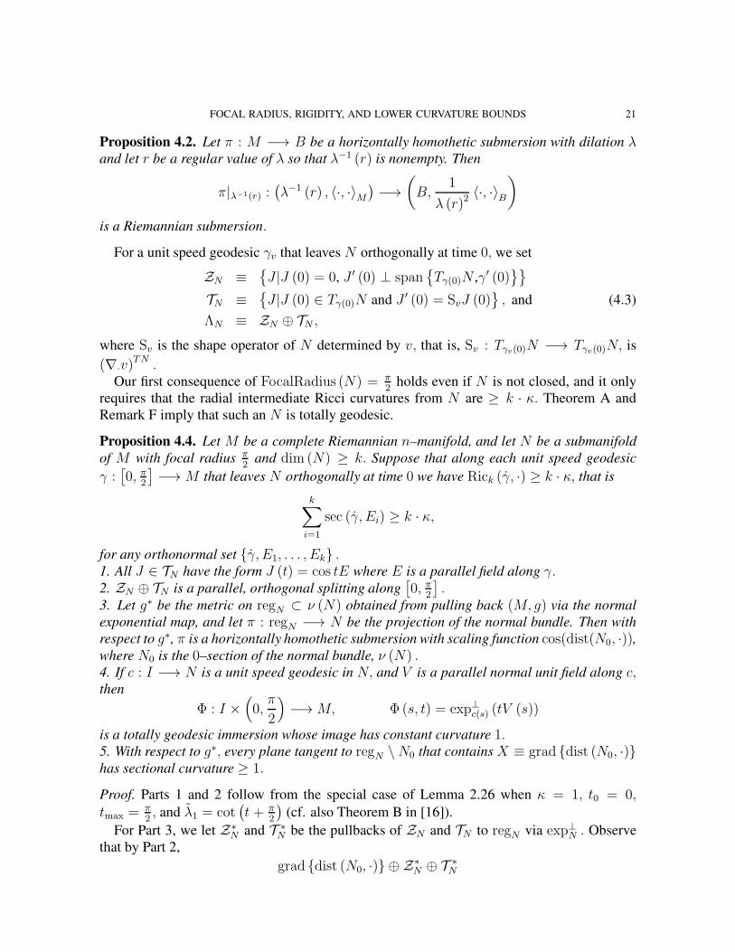
Proposition 4.2. Let π : M −→ B be a horizontally homothetic submersion with dilation λand let r be a regular value of λ so that λ−1 (r) is nonempty. Then

π|λ−1(r) :(λ−1 (r) , 〈·, ·〉M

)−→

(B,

1

λ (r)2〈·, ·〉B

)

is a Riemannian submersion.

For a unit speed geodesic γv that leaves N orthogonally at time 0, we set

ZN ≡{J |J (0) = 0, J ′ (0) ⊥ span

{Tγ(0)N ,γ′ (0)

}}

TN ≡{J |J (0) ∈ Tγ(0)N and J ′ (0) = SvJ (0)

}, and (4.3)

ΛN ≡ ZN ⊕ TN ,

where Sv is the shape operator of N determined by v, that is, Sv : Tγv(0)N −→ Tγv(0)N, is

(∇·v)TN .

Our first consequence of FocalRadius (N) = π2

holds even if N is not closed, and it only

requires that the radial intermediate Ricci curvatures from N are ≥ k · κ. Theorem A and

Remark F imply that such an N is totally geodesic.

Proposition 4.4. Let M be a complete Riemannian n–manifold, and let N be a submanifold

of M with focal radius π2

and dim (N) ≥ k. Suppose that along each unit speed geodesic

γ :[0, π

2

]−→ M that leaves N orthogonally at time 0 we have Rick (γ, ·) ≥ k · κ, that is

k∑

i=1

sec (γ, Ei) ≥ k · κ,

for any orthonormal set {γ, E1, . . . , Ek} .1. All J ∈ TN have the form J (t) = cos tE where E is a parallel field along γ.2. ZN ⊕ TN is a parallel, orthogonal splitting along

[0, π

2

].

3. Let g∗ be the metric on regN ⊂ ν (N) obtained from pulling back (M, g) via the normal

exponential map, and let π : regN −→ N be the projection of the normal bundle. Then with

respect to g∗, π is a horizontally homothetic submersion with scaling function cos(dist(N0, ·)),where N0 is the 0–section of the normal bundle, ν (N) .4. If c : I −→ N is a unit speed geodesic in N, and V is a parallel normal unit field along c,then

Φ : I ×(0,

π

2

)−→ M, Φ (s, t) = exp⊥

c(s) (tV (s))

is a totally geodesic immersion whose image has constant curvature 1.5. With respect to g∗, every plane tangent to regN \N0 that contains X ≡ grad {dist (N0, ·)}has sectional curvature ≥ 1.

Proof. Parts 1 and 2 follow from the special case of Lemma 2.26 when κ = 1, t0 = 0,tmax =

π2, and λ1 = cot

(t + π

2

)(cf. also Theorem B in [16]).

For Part 3, we let Z∗N and T ∗

N be the pullbacks of ZN and TN to regN via exp⊥N . Observe

that by Part 2,

grad {dist (N0, ·)} ⊕ Z∗

N ⊕ T ∗

N


is an orthogonal splitting of T regN with respect to g∗. Since the vertical space of π is spanned

by grad {dist (N0, ·)} ⊕ Z∗N , the horizontal space of π with respect to g∗ is spanned by T ∗

N .Since the fields of T ∗

N come from variations of geodesics that leave N0 orthogonally, they are

π–basic. Part 3 follows by combining this with Part 1.

For Part 4, observe that Part 1 gives us that Φ is an immersion. Let II be the second fun-

damental form of image (Φ) . By construction, ∂Φ∂t

is a geodesic field so II(∂Φ∂t, ∂Φ∂t

)= 0. It

follows from Part 1 that II(∂Φ∂t, ∂Φ∂s

)= 0.

To see that II(∂Φ∂s, ∂Φ∂s

)= 0, we note that, since ∂Φ

∂tis normal to exp⊥

N (S (N0, r)) , it suffices

to verify that

g

⟨II

(∂Φ

∂s,∂Φ

∂s

), Z

⟩= 0 (4.5)

for all Z ∈ T exp⊥N (S (N0, r)) that are normal to the image of Φ. Since exp⊥

N : (regN , g∗) −→

(M, g) is a local isometry, to prove (4.5), it suffices to do the corresponding calculation in

(regN , g∗) . From Part 3 we have that the restriction of π : (regN , g

∗) −→(N, 1

cos(t)2g)

to the

t–level set of dist(N0, ·) is a Riemannian submersion. Let ∂Φ∂s

be a lift of ∂Φ∂s

to regN via exp⊥N .

Then ∂Φ∂s

is a π–basic horizontal, geodesic field, so II(∂Φ∂s, ∂Φ∂s

)=

(D exp⊥

N

) (II(

∂Φ∂s, ∂Φ∂s

))≡

0. Hence the image (Φ) is totally geodesic. It follows from Part 1 that image (Φ) has constant

curvature 1.To prove Part 5, we let

{J∗1 , . . . , J

∗k−1

}be any k − 1 linearly independent Jacobi fields in

T ∗N . It follows from Part 1 that for all i,

sec (grad {dist (N0, ·)} , J∗

i ) ≡ 1.

Together with Part 2 and our hypothesis that Rick (γ, ·) ≥ k, we conclude that for all J∗ ∈Z∗

N , sec (grad {dist (N0, ·)} , J∗) ≥ 1.

It follows from Part 2 that Z∗N⊕T ∗

N is a splitting of ΛN0into orthogonal, invariant subspaces

for R (·, grad{dist (N0, ·)}) grad {dist (N0, ·)} . So

sec (grad {dist (N0, ·)} , Y ) ≥ 1

for all vectors Y orthogonal to grad {dist (N0, ·)} . �

5. THE STRUCTURE OF THE FOCAL SET

This section begins with a review of Hebda’s notion of regular tangent focal points that

generalizes a notion of Warner for conjugate points ([17], [30]). We next exploit the rigidity

in Proposition 4.4 to show that every tangent focal point at time π2

is regular. This allows us

to apply a result of Hebda and conclude that our focal set F ≡ exp⊥N

(S(N0,

π2

))is a smooth

submanifold of M. The rigid structure also yields that F has focal radius π2. We then further

the analogy between the pair (N,F ) and the dual sets in the proof of the Diameter Rigidity

Theorem by showing that F (resp. N) is the base of a Riemannian submersion from the unit

normal sphere to any point of N (resp. F ).

Definition 5.1. ([17], cf [30]) A tangent focal point v ∈ ν (N) is called regular if and only if

there is a neighborhood U of v so that every ray in ν (N) that intersects U has at most one

tangent focal point in U, not counting multiplicities. Otherwise v is called singular.


Continuity of the curvature tensor implies that every v ∈ ν (N) has a neighborhood U so

that every ray meeting U has the same number of tangent focal points, counting multiplicities.

So if v is a regular tangent focal point, then every ray tu in ν (N) that intersects U has exactly

one focal point t0u, and the multiplicities of t0u and v coincide. Thus regular tangent focal

points have locally maximal order. Using this and ideas of [30], Hebda showed the following.

Theorem 5.2. ([17], cf [30]) The set of regular tangent focal points is a smooth codimension

1 submanifold of ν (N) that is an open, dense subset of the set of all tangent focal points.

On regN ⊂ ν (N) , we set

X ≡ grad (dist (N0, ·)) .

Along a fixed geodesic, focal points are isolated, so it follows that the set of regular, first-

tangent focal points is an open, dense subset of the set of first-tangent focal points. It follows

from the Gauss Lemma that ker(D exp⊥

N

)X

⊥ X. Since the first-tangent focal set of our

N ⊂ M is S(N0,

π2

), it follows that ker

(D exp⊥

N

)⊂ TS

(N0,

π2

). Combining this with the

Rank Theorem we get

Corollary 5.3. Let Freg be the set of regular first-tangent focal points, and let

Freg ≡ exp⊥

N

(Freg

).

Then Freg is a smooth submanifold of M that is open and dense inside of F.

Lemma 5.4. Let v ∈ ν (N) be a singular tangent focal point. For every neighborhood U of

v, there is a regular tangent focal point w ∈ U so that

dim(ker

(D exp⊥

N

)w

)< dim

(ker

(D exp⊥

N

)v

).

Proof. Let U be any neighborhood of v. Replacing U with a possibly smaller neighborhood,

we may assume that the total multiplicity of the focal points on each ray that intersects U is

constant, and that the ray tv contains only one focal point in U . Since v is singular, U contains

a ray with more than one focal point w1 6= w2, which by hypothesis is not the ray through v.Since the multiplicity of the focal points in tw1 ∩ U and tv ∩ U is the same, it follows that

dim(ker

(D exp⊥

N

)w1

)< dim

(ker

(D exp⊥

N

)v

). (5.5)

It might be that w1 is not regular; however, since (5.5) holds for some w1 in any neighborhood

of v, by repeating this argument a finite number of times, we get the desired conclusion. �

Let γ be a unit speed geodesic that leaves N orthogonally at time 0 with γ(π2

)∈ Freg.

Recall that the elements of ΛN are called N–Jacobi fields. We set

Z ≡{J ∈ ΛN | J (0) = J

(π2

)= 0

},

TN ≡{J ∈ ΛN |J (0) ∈ Tγ(0)N and J ′ (0) = Sγ′(0) (J (0))

}, and

TFreg≡

{J | J

(π2

)∈ T

γ( π2 )Freg and J ′

(π2

)= −S

(J(π2

))},

where Sγ′(0) in the definition of TN is the shape operator of N and S in the definition of TFreg

is the Riccati operator of ΛN . The next lemma shows that the S in the definition of TFregis

also the shape operator of Freg with respect to γ′(π2

).


Lemma 5.6. For γ as above:

1. γ′(π2

)∈ ν

γ( π2 )Freg.

2. The N–Jacobi fields along γ are the Freg–Jacobi fields along

γ−1 : t 7→ γ(π2− t

).

3. The subspaces TN and TFregare rigid, that is,

TN = {cos t E| E is parallel and tangent to N at time 0} , and

TFreg=

{sin t E| E is parallel and tangent to Freg at time

π

2

}.

4. Writing ΛN for the N–Jacobi fields along γ, we have orthogonal splittings

ΛN = TN ⊕ TFreg⊕ Z and

ZN = TFreg⊕ Z,

where ZN is as in Equation (4.3).

Proof. Part 1 is a consequence of the Gauss Lemma and the fact that F ≡ exp⊥N

(S(N0,

π2

)).

The space ΛN of N–Jacobi fields along γ are precisely the variation fields of variations by

geodesics that leave N orthogonally at time 0. Similarly, the space ΛFregof Freg–Jacobi fields

along γ are precisely the variation fields of variations by geodesics that arrive at Freg or-

thogonally at time π2. It follows from Part 1 that ΛN ⊂ ΛFreg

. Since dim (ΛN) = n − 1 =

dim(ΛFreg

), ΛN = ΛFreg

. This proves Part 2.

Since γ has no focal points for N on(0, π

2

), it follows from Part 2 that γ−1 (t) = γ

(π2− t

)

has no focal points for Freg on(0, π

2

). By Part 5 of Proposition 4.4, all the radial sectional

curvatures along γ are ≥ 1. Thus Parts 3 and 4 follow from Parts 1 and 2 of Proposition 4.4

and the fact that γ−1 (t) = γ(π2− t

)has no focal points for Freg on

(0, π

2

). �

Lemma 5.7. Freg = F.

Proof. We set

Fsng ≡ F \ Freg,

and suppose, by way of contradiction, that Fsng 6= ∅.Let γreg and γsng be geodesics that leave N orthogonally at time 0 with

γreg

(π2

)∈ Freg and γsng

(π2

)∈ Fsng.

The idea of the proof is to examine how the splitting ZN = TFreg⊕Z behaves as a sequence

of γreg’s approaches γsng. In particular, by Lemma 5.6, TFregis spanned by constant curvature

1 Jacobi fields. By continuity, γsng inherits such a family, and this forces π2γ′sng (0) to actually

be regular. The details follow.

By appealing to Lemma 5.4, we can assume that

dim(ker

(D exp⊥

N

)π2γ′

reg(0)

)< dim

(ker

(D exp⊥

N

)π2γ′

sng(0)

). (5.8)

For either γreg or γsng we have the four spaces of Jacobi fields, ΛN , TN , ZN , and Z. We will

distinguish the versions of the spaces along γreg from those along γsng with the superscripts reg

and sng. When no superscript is present, the statement applies to either case.


For either γreg or γsng,

ker(D exp⊥

N

)π2γ′(0)

= {J (0) | J ∈ TN} ⊕ {J ′ (0) | J ∈ Z} . (5.9)

Thus

dim(ker

(D exp⊥

N

)π2γ′(0)

)= dim (TN) + dim (Z)

= dim (N) + dim (Z) .

Since dim(ker

(D exp⊥

N

)π2γ′

sng(0)

)> dim

(ker

(D exp⊥

N

)π2γ′

reg(0)

), the dimensions of Zreg

and Zsng satisfy

dim (Zsng) > dim (Zreg) . (5.10)

Along γreg, Lemma 5.6 gives us an orthogonal splitting

ZregN = T reg

Freg⊕ Zreg, (5.11)

where

T regFreg

={sin t E| E is parallel and tangent to Freg at time

π

2

}. (5.12)

Combined with Inequality (5.10), this gives

dim (Zsng) > dim (Zreg)

= dim (ZregN )− dim

(T regFreg

), by 5.11

= (n− 1)− dim (N)− dim(T regFreg

). (5.13)

Note that γsng is a limit of γreg’s that satisfy (5.8). Further note that a J ∈ T regFreg

together

with γ′reg spans a plane of constant curvature 1. Thus by continuity, Zsng

N contains a subspace

T sng of the form

T sng = {sin t E| E is parallel} ⊂ ZsngN \ Zsng

with

dim (T sng) = dim(T regFreg

). (5.14)

Moreover, by Remark 2.35, Part 2 of Lemma 2.23, and Part 5 of Proposition 4.4, ΛsngN splits

orthogonally with one factor being T sng. Since T sng is a subspace of ZsngN , we get

ZsngN = T sng ⊕ U sng, (5.15)

where U sng is a space of Jacobi fields in ZsngN that is orthogonal to T sng throughout

(0, π

2

).

The splitting (5.15) combined with T sng = {sin t E| E is parallel} gives that Zsng is a

subspace of U sng, so

dim (Zsng) ≤ dim (U sng)

= dim (ZsngN )− dim

(T regFreg

), by (5.14) and (5.15)

= (n− 1)− dim (N)− dim(T regFreg

).

Since this contradicts Inequality (5.13), the result is proven. �

Lemma 5.16. F is a totally geodesic closed submanifold of M with focal radius π2.


Proof. Since Freg = F, it is a submanifold. Since F = exp⊥N

(S(N0,

π2

)), it is closed. It

follows from Part 2 of Lemma 5.6 that ΛN = ΛF . Therefore the focal radius of F is π2.

We have F = Freg, so from Part 3 of Lemma 5.6,

TF ={sin t E| E is parallel and tangent to F at time

π

2

}.

In particular, for J ∈ TF , J′(π2

)= 0. So F is totally geodesic. �

The next result will lead to the spherical rigidity portion of the conclusion of Theorem B,

and also gives us Corollary C.

Theorem 5.17. M has constant curvature 1 if either of the following holds:

1. F is not connected.

2. dim(F ) + dim (N) = dim (M)− 1.

Proof. We have that exp⊥ : S(N0,

π2

)−→ F is onto. So if F is not connected, then S

(N0,

π2

)

is not connected, and it follows that N is codimension 1 and has a trivial normal bundle. Since

dim (F ) + dim (N) ≤ dim (ΛN) = dim (M)− 1,

to prove Part 1, it is enough to prove Part 2.

In general, we have an orthogonal splitting of ΛN = TN ⊕ TF ⊕ Z along any one of

our normal geodesics. Since dim (TF ) = dim (F ), dim (TN ) = dim (N) , and dim(F ) +dim (N) = dim (M)− 1, Z = 0, and our geodesic is spanned by constant curvature 1 Jacobi

fields. Moreover,

TN = ZF and TF = ZN .

Combining this with Part 1 of Proposition 4.4, it follows that along a geodesic leaving Forthogonally at time 0,

ZF = {sin tE | E is parallel} , (5.18)

and along a geodesic leaving N orthogonally at time 0,

ZN = {sin tE | E is parallel} . (5.19)

It follows from Equation (5.18) that for all x ∈ F and all r ∈(0, π

2

), the intrinsic metrics on

SF (x, r) ≡ exp⊥

x {v ∈ νx (F ) | |v| = r} (5.20)

are locally isometric to SdimN (sin r) , that is, to the sphere of radius sin r in RdimN+1. Simi-

larly, it follows that for all x ∈ N and all r ∈(0, π

2

), the intrinsic metrics on

SN (x, r) ≡ exp⊥

x {v ∈ νx (N) | |v| = r} (5.21)

are locally isometric to SdimF (sin r) . Since TN ⊕ZN is an orthogonal splitting, if γ leaves Northogonally at time 0, then

SN (γ (0) , r) and SF

(γ(π2

),π

2− r

)intersect orthogonally at γ (r) . (5.22)

Let

SN (r) ≡ exp⊥

N {v ∈ ν (N) | |v| = r} ,

and let IIr be the second fundamental form of SN (r) , that is

IIr (U, V ) ≡ g (∇UV, γ′ (r)) ,


where γ leaves N orthogonally at time 0.Combining (5.18), (5.19) and (5.22), we have for Y ∈ TN , and W ∈ ZN ,

IIr (Y, Y ) = |Y |2 tan (r)

IIr (W,W ) = − |W |2 cot (r) , and

IIr (Y,W ) = 0. (5.23)

Now view Sn as a join, Sn = SdimN ∗ SdimF, and let γ be a geodesic that leaves SdimN

orthogonally at time 0. Setting M ≡ Sn, N ≡ SdimN, and F ≡ SdimF, observe that (5.20),

(5.21), (5.22), and (5.23) hold with M , N, and F replaced by M , N , and F . Observe fur-

ther that Equations (5.20), (5.21), (5.22), and (5.23) together with the Gauss, Radial, and

Codazzi-Mainardi Equations ([23]) determine the curvature tensor of M ≡ Sn. Similarly,

they determine the curvature tensor of M. Thus M has constant curvature 1. �

Throughout the remainder of Part 2, we assume that F is connected and

dim (F ) + dim (N) ≤ dim (M)− 2. (5.24)

Lemma 5.25. 1. Let x ∈ N. With respect to the constant curvature 1 metric on the unit normal

sphere, ν1x (N) , the map

πx : ν1x (N) −→ F

πx : v 7→ expN

(π2v)

is a Riemannian submersion onto F.2. Let x ∈ F. With respect to the constant curvature 1 metric on the unit normal sphere,

ν1x (F ) , the map

πx : ν1x (F ) −→ N

πx : v 7→ expF

(π2v)

is a Riemannian submersion onto N.

Proof. The proofs are identical, except for notation . We give the details for Part 1.

Let γ be a geodesic that leaves N orthogonally at time 0. Then

Tγ′(0)

(ν1γ(0) (N)

)= {J ′ (0) | J ∈ ZN} , and

Dπγ(0) (J′ (0)) = J

(π2

)(5.26)

for all J ∈ ZN .Since TF ⊂ ZN , the splittings ΛN = TN ⊕ ZN = TN ⊕ TF ⊕ Z give us an orthogonal

splitting

ZN = Z ⊕ TF .

Combined with Equation (5.26) this gives an orthogonal splitting

Tγ′(0)

(ν1γ(0) (N)

)= {J ′ (0) | J ∈ Z} ⊕ {J ′ (0) | J ∈ TF} (5.27)

into the vertical and horizontal spaces, respectively, for πγ(0). Since dim (TF ) = dim (F ) , it

follows from Equation (5.26) that πγ(0) is a submersion. By Part 1 of Proposition 4.4, with F


playing the role of N, the restriction of Dπγ(0) to the second summand in Equation (5.27) is

an isometry. Thus πγ(0) is a Riemannian submersion. �

6. THE SIMPLY CONNECTED CASE

Let π : M −→ M be the universal cover of M . Then each component π−1 (N) is a

submanifold with focal radius π2

and dimension at least k. In particular, M contains a closed,

connected, embedded submanifold with focal radius π2

and dimension at least k. So to prove

Theorem B, it suffices to consider the case when M is simply connected and N is connected.

In this section, we will combine our simply connected hypothesis with Hebda’s theorem on

“very regular” focal loci. This will allow us to assert that, topologically, M is the union of two

disk bundles, and the fibers of our Riemannian submersions,

πx : ν1x (N) −→ F

πx : v 7→ expN

(π2v)

and

πx : ν1x (F ) −→ N

πx : v 7→ expF

(π2v)

are connected. We start with a review of Hebda’s result.

Definition 6.1. (Hebda, [17]) Consider geodesics γ that leave N orthogonally at time 0. Nhas a very regular first focal locus if the multiplicity of the first focal point is independent of

γ and, in case the multiplicity is one, ker(D exp⊥

N

)is contained in the tangent space to the

tangent focal locus at every first-tangent focal point.

Along a geodesic that leaves our N orthogonally at time 0, the multiplicity of the focal point

at time π2

is

dimZF = dim (ΛN)− dim TF

= dim (M)− 1− dim (F ) ,

and hence is constant. Since the focal radius of N along every geodesic is π2, it follows from

the Gauss Lemma that our N has a very regular first focal locus. Therefore, since M is simply

connected, we can apply the following result of Hebda. (See Theorem 3.1 in [17] and the first

line of its proof.)

Theorem 6.2. (Hebda, [17]) Suppose M is a connected, compact Riemannian manifold, and

N is a connected, compact submanifold having a very regular first focal locus such that the

inclusion ι : N → M induces a surjection of fundamental groups.

If the multiplicity of the first focal points of N is s−1, then the first focal locus F of N in Mis a submanifold of codimension s that coincides with the cut locus of N in M. Moreover, the

tangent cut locus of N coincides with the first-tangent focal locus of N, and M is the union of

two disk bundles

M = DN ∪ϕ DF


over N and F respectively, where

ϕ : ∂DN −→ ∂DF

is a diffeomorphism.

By combining transversality and Theorem 6.2 we get following.

Corollary 6.3. Suppose that M is simply connected.

1. If codim(F ) ≥ 3, then N is simply connected.

2. If codim(N) ≥ 3, then F is simply connected.

Proof. The two statements have dual proofs. We give the details for Part 1.

Transversality gives us

π1 (M) ∼= π1 (M \ F ) ,

and by Theorem 6.2, M \ F deformation retracts to N. �

Similarly, the cut locus statements in Theorem 6.2 gives us

Corollary 6.4. If M is simply connected, then exp⊥N is injective on B

(N0,

π2

).

Lemma 6.5. Let M be simply connected.

1. If codim(N) ≥ 3, then the Riemannian submersions

ν1x (N) −→ F, x ∈ N

have connected fibers with positive dimension.

2. If codim(F ) ≥ 3, then the Riemannian submersions

ν1x (F ) −→ N, x ∈ F

have connected fibers with positive dimension.

Proof. Since we have assumed that dim (F ) + dim (N) ≤ dim (M)− 2,

dim(ν1x (N)

)= dim (M)− dim (N)− 1

> dim (F ) .

Thus the fibers of ν1x (N) −→ F have positive dimension.

By Corollary 6.3, F is simply connected if codim(N) ≥ 3. In this case, the long exact

homotopy sequence for ν1x (N) −→ F, x ∈ N gives

π1 (F ) −→ π0 (fiber) −→ 0,

since π0 (ν1x (N)) is trivial. Thus the first conclusion holds. A similar argument gives us the

second conclusion, if codim(F ) ≥ 3. �

Since we have assumed that

dim (F ) + dim (N) ≤ dim (M)− 2, (6.6)

codim(N) ≥ 2. Since dim (N) ≥ 1, we have codim(F ) ≥ 3. Combining this with Lemma

5.16, Corollary 6.4, and Lemma 6.5, we have


Theorem 6.7. Let M be a complete Riemannian n–manifold with Rick ≥ k and N any closed,

connected, submanifold of M with dim (N) ≥ k and focal radius π2. If M is simply connected

and not isometric to the unit sphere, then:

1.

dim (N) + dim (F ) ≤ n− 2.

2. N is totally geodesic and isometric to an even dimensional CROSS.3. The focal set F of N is totally geodesic and is either a point or is isometric to an even

dimensional CROSS.

4. The normal exponential maps of N and F are injective on the π2–balls around the zero

sections of the normal bundles of N and F.5. The conclusions of Proposition 4.4 hold with N replaced by F.6. For every x ∈ F the map

πx : ν1x (F ) −→ N

πx : v 7→ expN

(π2v)

is a Riemannian submersion whose fibers are connected and have positive dimension.

7. For every x ∈ N the map

πx : ν1x (N) −→ F

πx : v 7→ expN

(π2v)

is a Riemannian submersion whose fibers are connected and have positive dimension.

7. RIGIDITY IN THE SECTIONAL CURVATURE CASE

In this section, we complete the proof of Theorem B in the case when the sectional curvature

of M is ≥ 1. Since M is simply connected, by Part 4 of Theorem 6.7, the diameter of M is

≥ π2. So combining the Diameter Rigidity Theorem with our dimension hypothesis (6.6) and

Theorem 6.7 gives us the following.

Proposition 7.1. If M does not have constant curvature 1, then the following hold.

1. M is isometric to a compact, rank one, symmetric space or is homeomorphic to Sn.2. N is even dimensional and isometric to the base of a Hopf fibration.

3. F is either a point or is isometric to the base of a Hopf fibration and is even dimensional

To conclude the proof of Theorem B, we show that conclusions 2 and 3 are not compatible

with M being a topological sphere.

If M is a sphere, the long exact homology sequence of the pair (M,F ) gives

Hq (M,F ) ∼= H#q−1 (F )

for q ≤ n− 1.Use Theorem 6.2 to write

M = DN ∪ϕ DF .

By excision,

Hq (M,F ) ∼= Hq (DN , ∂DN) .


Thus for q ≤ n− 1,

H#q−1 (F ) ∼= Hq (DN , ∂DN ) . (7.2)

By Proposition 7.1, F is either an even dimensional CROSS or a point, and N is an even

dimensional CROSS. It follows from Equation (7.2) that Hq (DN , ∂DN) ∼= 0 if q is even and

≤ n− 1. If q is odd and q + 1 ≤ n− 1, then the sequence of the pair (DN , ∂DN ) gives

0 = Hq+1 (DN , ∂DN ) −→ Hq (∂DN ) −→ Hq (N) = 0,

since N is an even dimensional CROSS. Thus

Hq (∂DN ) ∼= 0 if q is odd and ≤ n− 2. (7.3)

Since N is isometric to the base of a Hopf fibration with connected fibers, dim (N) ≥ 2.Since dim (N) + dim (F ) ≤ n − 2, we get n ≥ 4. So dim (∂DN ) ≥ 3. Since ∂DN is

a connected, compact, odd dimensional manifold, (7.3) implies, via Poincare duality, that

∂DN is a Z2–homology sphere of dimension ≥ 3 . Thus the Mayer–Vietoris sequence with

q ∈ {2, . . . , n− 2} yields

0 = Hq (∂DN ) −→ Hq (DN)⊕Hq (DF ) −→ Hq (M) −→ Hq (∂DN ) = 0.

Since DN has the homotopy type of the CROSS N, and dim (M) ≥ dim (N) + 2 ≥ 4, Mcannot be homeomorphic to a sphere.

8. RIGIDITY AND INTERMEDIATE RICCI

In this section, we complete the proof of Theorem B. This is achieved by analyzing the radial

geometry from N and F. Proposition 4.4, Lemma 5.6, and Lemma 5.16 give us rigid radial

geometry along the distribution spanned by the Jacobi fields in TN and TF . To prove rigidity

for the Z–Jacobi fields, we show, in Proposition 8.8, that as in the proof of the Diameter

Rigidity Theorem, there are enough other dual pairs in M to force the Z–Jacobi fields to span

projective lines. This is achieved via the next three results, wherein the hypotheses that N is

connected and M is simply connected are still in force.

Proposition 8.1. 1. For any p ∈ N the cut point along any geodesic emanating from p is at

distance π2

from p.2. For any p, q ∈ N, any minimal geodesic of M between p and q lies entirely in N.

Proof. Let v ∈ TpM \{TpN, νp (N)} be any unit vector. Let vT and v⊥ be the unit vectors that

point in the same directions as the projections of v onto TpN and νp (N) , respectively. By Part

4 of Proposition 4.4, span{vT , v⊥

}exponentiates to a totally geodesic immersed surface Σ of

constant curvature 1 that contains γv. By Corollary 6.4, the restriction of expp to the interior

of the circular sector

Sect(vT , v⊥,

π

2

)≡

{expp

(t(vT cos s+ v⊥ sin s

)) ∣∣ t, s ∈[0,

π

2

]}

of radius and angle π2

spanned by vT and v⊥ is an embedding. If w ∈ TpM is not in

TpN, νp (N) , or span{vT , v⊥

}, then Corollary 6.4 gives that interiors of Sect

(vT , v⊥, π

2

)and

Sect(wT , w⊥, π

2

)are disjoint. It follows that the cut-time of any unit v ∈ TpM\{TpN, νp (N)}

is ≥ π2, and by continuity, the cut-time of any unit v ∈ TpM is ≥ π

2.


Since the focal radius of N is π2, to complete the proof of Part 1, it suffices to check that any

unit v ∈ TpM \ νp (N) has a cut point at time π2. Since N is a CROSS with curvature in [1, 4] ,

there is a unit vector wT ∈ Tp (N) with

γwT

(π2

)= γvT

(π2

)and wT 6= vT .

Let u ∈ νγvT (

π2 )

(N) be a unit vector. Let Uv and Uw be the backwards parallel transports of

u along γvT and γwT . Let ΣvT and ΣwT be the spherical sectors of radius and angle π2

obtained

via Part 4 of Proposition 4.4 by exponentiating Uv and Uw. That is

ΣvT ≡{expN (tUv (s)) | s, t ∈

[0,

π

2

]}

and

ΣwT ≡{expN (tUw (s)) | s, t ∈

[0,

π

2

]}.

Then ΣwT and ΣvT are different surfaces, but since

Uv

(π2

)= Uw

(π2

)= u ∈ ν

γvT (

π2 )

(N) ,

ΣwT and ΣvT intersect along expN (tu) . So every cut point from p occurs at distance π2

from

p.By Corollary 6.4, the intersection of N with any of the sectors Sect

(vT , v⊥, π

2

)is precisely

γvT[0, π

2

]⊂ N. Part 2 follows. �

Proposition 8.2. For any p ∈ N, the set of points in M at distance π2

from p,

A (p) ≡ S(p,

π

2

),

is a closed submanifold of dimension

dim (N) + dimF

and focal radius π2.

Proof. Let

AN (p) ≡{x ∈ N | dist (p, x) =

π

2

}.

Using the rigid hinges of Part 4 of Proposition 4.4 and the fact that A (p) ≡ S(p, π

2

)is the cut

locus of p we see that we can describe A (p) in two ways:

A (p) ={exp⊥

N (tv)∣∣ v ∈ ν1 (N) |AN (p) and t ∈

[0,

π

2

]},

and

A (p) ={exp⊥

F (tv)∣∣ v ∈ ν1 (F ) , expF

(π2v)∈ AN (p) , and t ∈

[0,

π

2

]}. (8.3)

Either description shows A (p) is compact. Since both N and F have focal radius π2, both

descriptions show, via Corollary 6.4, that A (p) \ {F ∪N} is a manifold. The first description

shows that A (p) is smooth near N .


Recall that for every x ∈ F, the map

πx : ν1x (F ) −→ N,

πx : v 7→ expN

(π2v)

is a Riemannian submersion with connected fibers. Combining this with Part 4 of Proposition

4.4 and Proposition 8.1, we rewrite (8.3) as

A (p) = ∪x∈F

{exp⊥

F (tv)∣∣ v ∈ ν1

x (F ) , v ⊥ π−1x (p) , and t ∈

[0,

π

2

]}, (8.4)

where {v} and π−1x (p) are subsets of νx (F ) , and the notion of perpendicular comes from the

inner product that g induces on νx (F ) . This shows A (p) is smooth near F.Next, we decompose ν1

x (F ) as a join

ν1x (F ) = π−1

x (p) ∗(π−1x (p)

)⊥, where

(π−1x (p)

)⊥≡

{v ∈ ν1

x (F )∣∣ v ⊥ π−1

x (p)}.

Note that (8.4) gives that for any x ∈ F ,

dim (A (p)) = dimF + dim(π−1x (p)

)⊥+ 1. (8.5)

Since πx : ν1x (F ) −→ N is a Riemannian submersion,

dim (N) = dim(Hv

(π−1x (p)

)), (8.6)

where Hv (π−1x (p)) is the horizontal space for πx at any v ∈ π−1

x (p) ⊂ ν1x (F ) .

The join decomposition ν1x (F ) = π−1

x (p) ∗ (π−1x (p))

⊥identifies (π−1

x (p))⊥

with the unit

vectors in Hv (π−1x (p)) . So

dim(π−1x (p)

)⊥= dim

(Hv

(π−1x (p)

))− 1.

Combining with Equations (8.5) and (8.6), we get

dim (A (p)) = dimF + dim (N)− 1 + 1.

Since A (p) = S(p, π

2

)is a smooth submanifold, and every geodesic that leaves p has cut

point at distance π2

from p, it follows from 1st–variation that every geodesic leaving p arrives

orthogonally at A (p) at time π2. This identifies the unit tangent sphere at p, Sp, with the unit

normal bundle of A (p) , ν1 (A (p)) . Combined with Proposition 8.1, it follows that the focal

radius of A (p) along any normal geodesic is greater than or equal to π2

. So it follows from

Theorem A that the focal radius of A (p) is exactly π2. �

It follows that Theorem 6.7 applies with Np = A (p) and F p = p.Next, we apply Propositions 8.1 and 8.2 to q ∈ A (p) and, with a further application of

Theorem 6.7, get the following result.

Proposition 8.7. 1. Every cut point from q occurs at distance π2

from q.2. The set of points in M at distance π

2from q,

A (q) ≡ S(q,

π

2

),

is a closed submanifold with focal radius π2

and dimension dimN + dimF.


3. A (q) is totally geodesic and isometric to a CROSS.

4. For any a, b ∈ A (q) , any minimal geodesic of M between a and b lies entirely in A (q) .

Returning Np = A (p) and F p = p, we now have the following refinement of Proposition

4.4.

Proposition 8.8. Let γ be a unit speed geodesic that leaves Np orthogonally at time 0 and let

ΛNp, TNp and ZNp be as in (4.3).

1. ZNp ⊕ TNp is a parallel, orthogonal splitting of ΛNp along(0, π

2

).

2. TNp and ZNp have the forms

TNp ≡ {cos tE| E is parallel and tangent to Np at time 0} ,

ZNp ≡

{1

2sin 2tE| E is parallel and orthogonal to Np at time 0

}.

Proof. Apart from the second equation in Part 2, this is a repeat of Parts 1 and 2 of Proposition

4.4. The second equation in Part 2 follows from Part 2 of Proposition 8.7. Indeed, let γ be

a unit speed geodesic from x ∈ Np to p. Choose q ∈ Np at distance π2

from x, and apply

Proposition 8.7 to q. It follows that γ ⊂ A (q) , and A (q) is a totally geodesic CROSS. In

particular, the Jacobi fields along γ have the indicated form if they are tangent to A (q) . Since

the normal space to A (q) along γ is spanned by a subspace of TNp, the result follows. �

We finish the proof of Theorem B along the lines of the proof of Theorem 4.3 in [14] by

using Cartan’s Theorem (Theorem 2.1, page 157 of [7]).

Since Theorem 6.7 applies to Np = A (p) , there is a CROSS P with

dim (P ) = dim (M)

and

dim (ZNp) = dim (F)− 1,

where F is the division algebra that defines P.Choose a point p ∈ P. Since P is a CROSS, we have a Riemannian submersion

πp : Sp −→ A (p) ≡{x ∈ P | dist (x, P ) =

π

2

}

that is isometrically equivalent to a Hopf Fibration. Since dim (ZNp) = dim (F)−1, we have,

using [13] and [32], that πp is isometrically equivalent to

πp : Sp −→ Np ≡ A (p) .

Let

I : Sp −→ Sp

be a linear isometric equivalence between πp and πp. Then we have a commutative diagram

SpI

−→ Sp

↓ πp ↓ πp

A (p)I

−→ A (p)

Since πp and πp are Riemannian submersions and I is an isometry, I is an isometry.


Via the Cartan Theorem and Proposition 8.8, we see that ι ≡ expp ◦I ◦ exp−1p defines an

isometry between P\ A (p) and M \A (p) that induces the isometry I : A (p) −→ A (p) , and

thus ι extends to an isometry P −→ M. This completes the proof of Theorem B.

REFERENCES

[1] P. Baird and J. Eells, A conservation law for harmonic maps, E. Looijenga, D. Siersma, and F. Takens,

editors, Geometry Symposium. Utrecht 1980, volume 894 of Lecture Notes in Math., Springer, Berlin,

Heidelberg, New York, 1981, pp. 1–25.

[2] P. Baird and J. C. Wood, Harmonic morphisms between Riemannian manifolds, London Math. Soc. Monogr.

(N.S.) No. 29, Oxford Univ. Press (2003).

[3] J. Cheeger and D. Ebin, Comparison Theorems in Riemannian Geometry, North-Holland, 1975.

[4] J. Cheeger and D. Gromoll, The splitting theorem for manifolds of nonnegative Ricci curvature, Journ. Diff.

Geom. 6 (1971) 119-128.

[5] S. Cheng, Eigenvalue comparison theorems and its geometric applications, Mathematische Zeitschrift 143,

no. 3 (1975), 289–297.

[6] C. Croke and B. Kleiner, A warped product splitting theorem, Duke Math. J. 67 (1992) 571-574.

[7] M. do Carmo, Riemannian Geometry, Mathematics: Theory and Applications. Birkhauser Boston, Inc.,

Boston, MA, (1992).

[8] J.H. Eschenburg, Comparison theorems and hypersurfaces, Manuscripta Math. 59 (1987), no 3, 295-323.

[9] J.H. Eschenburg and E. Heintze, Comparison theory for Riccati equations, Manuscripta Math. 68 (1990),

no. 2, 209–214.

[10] J.H. Eschenburg and J. O’Sullivan, Jacobi Tensors and Ricci Curvature, Math. Ann. 252 (1980), no. 1,

1–26.

[11] D. Gonzalez-Alvaro and L. Guijarro, Soft restrictions on positively curved Riemannian submersions, Jour-

nal of Geometric Analysis, 26 (2016), no. 2, 1442–1452.

[12] A. Gray, Pseudo-Riemannian almost product manifolds and submersions, J. Math. Mech. 16 (1967), 413–

443.

[13] D. Gromoll and K. Grove, The low-dimensional metric foliations of Euclidean spheres, J. Differential

Geometry 28, (1988), 143-156.

[14] D. Gromoll and K. Grove, A generalization of Berger’s rigidity theorem for positively curved manifolds,

Ann. Sci. Ecole Norm. Sup., 4 serie, t. 20, 227-239.

[15] D. Gromoll and G. Walschap, Metric foliations and curvature, Progress in Mathematics 268, Birkhauser

Verlag, Basel, 2009.

[16] D. Gumaer and F. Wilhelm, On Jacobi field splitting theorems, Differential Geometry and its Applications

37 (2014) 109–119.

[17] J. Hebda, The regular focal locus, J. Diff. Geom. 16 (1981) 421-429.

[18] E. Heintze and H. Karcher, A general comparison theorem with applications to volume estimates for sub-

manifolds, Ann. Sci. Ecole Norm. Sup. 11 (1978), no. 4, 451–470.

[19] A. Lytchak, Notes on the Jacobi equation, Differential Geom. Appl. 27 (2009), no. 2, 329–334.

[20] S. Myers, Riemannian manifolds with positive mean curvature, Duke Mathematical Journal 8, no. 2 (1941),

401–404.

[21] B. O’Neill, The fundamental equations of a submersion, Michigan Math. J. 13 (1966), 459–469.

[22] Y. Ou and F. Wilhelm, Horizontally homothetic submersions and nonnegative curvature, Indiana University

Mathematics Journal 56 (2007) 243-262.

[23] P. Petersen, Riemannian Geometry, 2nd Ed., New York: Springer Verlag, 2006.

[24] B. Schmidt, Positively curved manifolds with large conjugate radius, J. Topol. Anal. 5 (2013), no. 3, 333–

344.

[25] C. Searle and F. Wilhelm, How to lift positive Ricci curvature, Geometry and Topology 19 (2015), 1409–

1475.


[26] K. Shankar, R. Spatzier, and B. Wilking, Spherical rank rigidity and Blaschke manifolds, Duke Math. J..

128 (2005), no.1, 65-81.

[27] Z. Shen, A sphere theorem for positive Ricci curvature, Indiana Univer. Math. J. 38, (1989), 229-233.

[28] L.Verdiani and W.Ziller, Concavity and rigidity in non-negative curvature, J. Diff. Geom. 97(2014), no. 2,

349–375.

[29] F. Warner, Extension of the Rauch Comparison Theorem to Submanifolds, Transactions of the American

Mathematical Society 122, No. 2 (1966), 341-356.

[30] F. W. Warner, The conjugate locus of a Riemannian manifold, Amer. J. Math. 87 (1965) 575-604.

[31] B. Wilking, A duality theorem for Riemannian foliations in nonnegative sectional curvature, Geom. Funct.

Anal. 17 (2007), 1297–1320.

[32] B.Wilking, Index parity of closed geodesics and rigidity of Hopf fibrations, Invent. Math. 144 (2001), 281–

295.

[33] H. Wu, Manifolds of partially positive curvature, Indiana Univ. Math. J. 36, (1987), 525-548.

DEPARTMENT OF MATHEMATICS, UNIVERSIDAD AUTONOMA DE MADRID, AND ICMAT CSIC-UAM-

UCM-UC3M

E-mail address: [email protected]

URL: http://www.uam.es/luis.guijarro

DEPARTMENT OF MATHEMATICS, UNIVERSITY OF CALIFORNIA, RIVERSIDE, CA 92521

E-mail address: [email protected]

URL: https://sites.google.com/site/frederickhwilhelmjr/home

LUIS GUIJARRO AND FREDERICK WILHELM … · Theorem B implies that the standard unit metric is the...

Documents

Transcript of LUIS GUIJARRO AND FREDERICK WILHELM … · Theorem B implies that the standard unit metric is the...