Luis G. VargasDecision, Operations and Information Technologies

The Joseph M. Katz Graduate School of BusinessUniversity of Pittsburgh

lgvargas@pitt.edu

2

Definition of FORECASTtransitive verb1a : to calculate or predict (some future event or condition) usually as a result of study and analysis of available pertinent data; especially : to predict (weather conditions) on the basis of correlated meteorological observationsb : to indicate as likely to occur2: to serve as a forecast of : PRESAGE <such events mayforecast peace>intransitive verb: to calculate the future— fore·cast·able adjective— fore·cast·er noun

3

Forecasting is the prediction of the future of a system using past information.

Forecasting implies the use of past information. How back into the past depends on the application.

Prediction on the other hand does not need the past, e.g., the best predictor of tomorrow’stock price is today’s price.

4

5

The Economist Intelligence Unit and CFO Research conducted a global survey of 544 senior executives. Thirty-five percent of respondents were based in Europe, 30 percent in the Americas and 29 percent in Asia Pacific. The survey reached a very senioraudience; over 30 percent of respondents were CFOs. Fifty-nine percent of respondents were from organizations with over US$1 billion dollars in annual revenues and respondents were drawn from a cross-section of industries.

© 2007 KPMG International

6

Although forecasting is traditionally considered a “financial exercise,” leading organizations widely acknowledge that it is at the heart of the performance management process and potentially a significant driver of business value and investor confidence.All organizations use forecasts to predict and manage their future performance. But although organizations invest significant time and effort in this important task, only one in five currently produce a forecast that is reliable.

7

The survey results were segmented and analyzed in various ways to shed light on whether top performing organizations take a different approach to forecasting.

In particular, the report analyses responses from organizations with high levels of forecast accuracy (within five percent of actual results over the past three years) compared to those that had a wider margin of error when forecasting over the past three years.

To supplement the survey, the Economist Intelligence Unit conducted a program of interviews with senior executives as well as academics and experts in the field.

8

Over the last three years,

◦ Accurate 1%◦ Within 5% 22%

Avg increase in stock price 46%◦ Others

Avg increase in stock price 34%

◦ Avg error 13%

9

Automation (IT tools)Scenario planning/sensitivity analysisRolling forecastsReduction in detailQuality of data

10

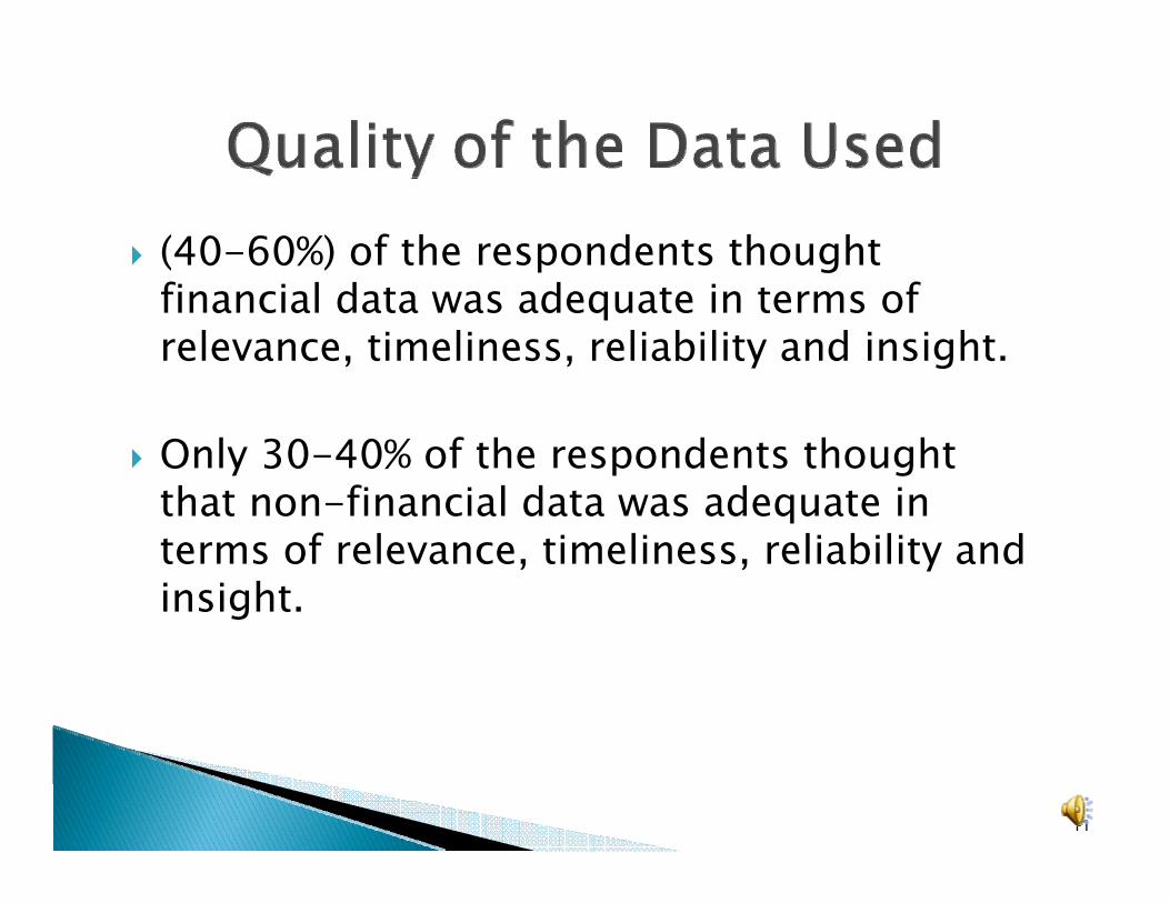
(40-60%) of the respondents thought financial data was adequate in terms of relevance, timeliness, reliability and insight.

Only 30-40% of the respondents thought that non-financial data was adequate in terms of relevance, timeliness, reliability and insight.

11

40% of the companies use spreadsheets28% use more accurate tools44% use low technology tools

12

Dedicated forecasting team (12%)Mainly finance dept. (23%)Mixed finance dept. (26%)Finance, sales, marketing, supply chain and others (34%)

13

The survey suggests that companies are much more likely to outperform rather then underperform their predictions, with the average forecast coming out eight percent below actual.

14

They take forecasting more seriously◦ Accountability, incentives, ongoing performance,

earnings guidanceThey look to enhance quality beyond the basics◦ Scenario planning and sensitivity analysisThey leverage information more effectively◦ External reporting, quality of data, use op. mgrs.They work harder at it◦ Use more sophisticate tools, update more oftenThey benefit the shareholders

15

Benefits of Collaborative forecasting◦ Lower inventories and capacity buffers◦ Fewer unplanned shipments or production runs◦ Reduced stock-outs◦ Increase customer satisfaction and repeat business◦ Better preparation for sales promotions◦ Better preparation for new product introductions◦ Dynamically respond to market changesThe Beer Game (http://www.masystem.com/o.o.i.s/1365)

16

Principles of Forecasting: A Handbook for Researchers and Practitioners, edited by J. Scott Armstrong. Kluwer Academic Publishers, 2001. This book can be used in conjunction with the website http://forecastingprinciples.com

139 principles to consider when building a forecast.

17

Depending on the type of information used they can be classified into:

◦ Classical forecasting – using dataSmoothing, time series, regression, ARIMA

◦ Judgmental forecasting – using knowledgeSurveys, Delphi method, scenarios, analogy, AHP/NP

◦ Hybrid forecasting – using both data and knowledge

Artificial intelligence, neural nets, data mining

18

19

Business Forecasting, 6th Edition, J. Holton Wilson, Barry Keating, John Galt Solutions, Inc. McGraw-Hill, 2009.

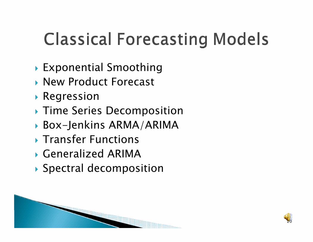
Exponential SmoothingNew Product ForecastRegressionTime Series DecompositionBox-Jenkins ARMA/ARIMATransfer FunctionsGeneralized ARIMA Spectral decomposition

20

Moving Averages

Simple (stationary series)

Double (series with trend)

1 (1 )t t tF X Fα α+ = + −

1( ) nX XMA nn

+ +=

L

1 (1 )( )t t t tF X F Tα α+ = + − +

1 1( ) (1 )t t t tT F F Tβ β+ += − + −

1 1t m t tH F mT+ + += +

21

Triple (series with trend and seasonality)

( )t m t t t m pW F mT S+ + −= +

1 1( ) (1 )t t t tT F F Tβ β− −= − + −

1 1/ (1 )( )t t t p t tF X S F Tα α− − −= + − +

/ (1 )t t t t pS X F Sγ γ −= + −

22

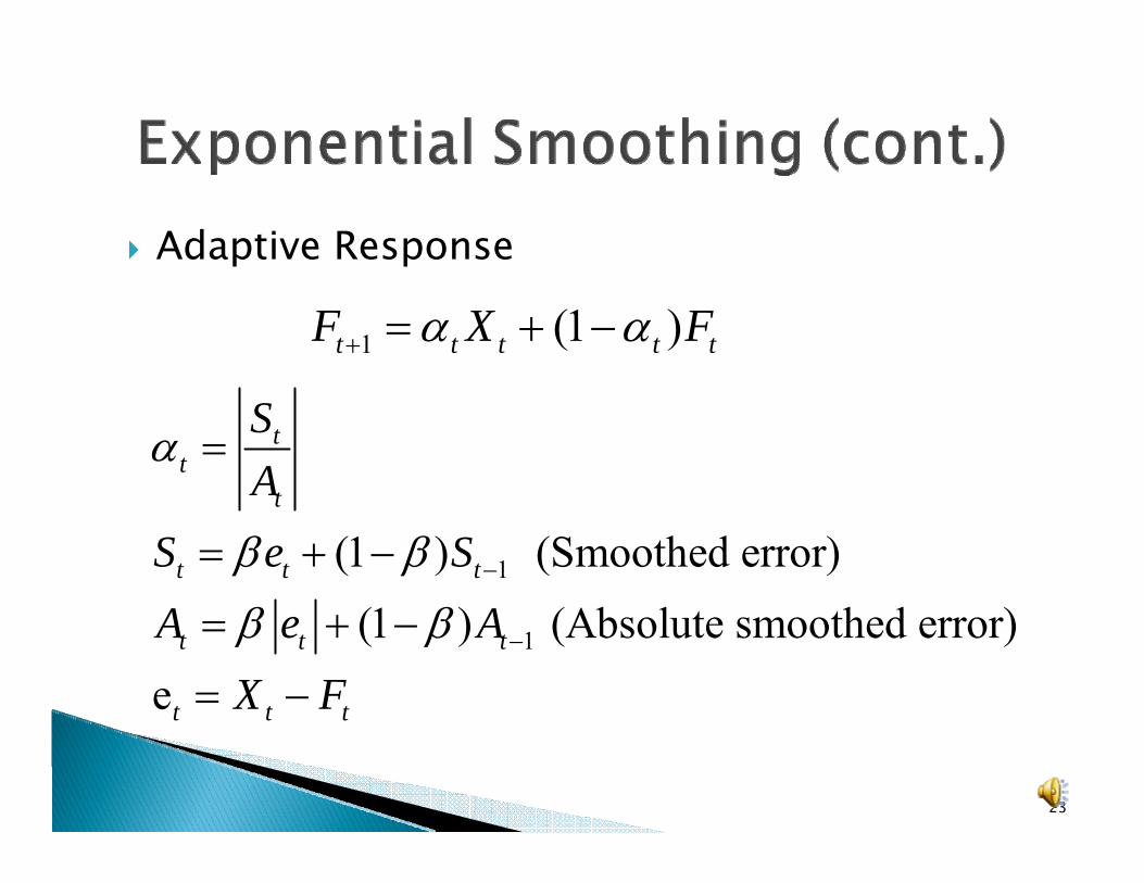
Adaptive Response

1

1

(1 ) (Smoothed error)(1 ) (Absolute smoothed error)

e

tt

t

t t t

t t t

t t t

SA

S e SA e A

X F

α

β ββ β

−

−

=

= + −

= + −

= −

1 (1 )t t t t tF X Fα α+ = + −

23

24

25

26

27

28

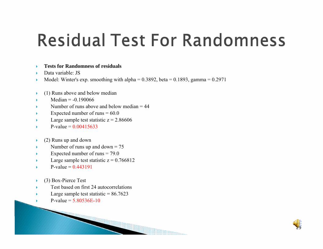
Tests for Randomness of residualsData variable: JSModel: Winter's exp. smoothing with alpha = 0.3892, beta = 0.1893, gamma = 0.2971

(1) Runs above and below medianMedian = -0.190066Number of runs above and below median = 44Expected number of runs = 60.0Large sample test statistic z = 2.86606P-value = 0.00415633

(2) Runs up and downNumber of runs up and down = 75Expected number of runs = 79.0Large sample test statistic z = 0.766812P-value = 0.443191

(3) Box-Pierce TestTest based on first 24 autocorrelationsLarge sample test statistic = 86.7623P-value = 5.80536E-10

29

Gompertz Curve

Logistics Curve

btaetY Le

−−=

1t bt

LYae−=

+

30

Bass Model

( ) rate of change of the installed base fraction( ) installed base fraction

A(t) cumulative adopter function coefficient of innovation coefficient of imitation potential market

f tF t

pqM

( )

( )

1( )1

p q t

p q t

eF t q ep

− +

− +

−=

+

( ) ( ), 0( ) ( )

( ) 1( )

( ) ( 1) 1

A t MF t ta t Mf t

F t tf t

F t F t t

= >=

=⎧= ⎨ − − >⎩

( ) ( )1 ( )

f t qp A tF t M

= +−

31

Simple regression (usually to determine the trend of the series)

Multiple Regression

Seasonality can be incorporated with dummy variables, but the seasonality length must be known for accuracy

32

0 10

0 1

ˆ ˆ

ˆ ˆt t t

t t

Y X e

X t e

β β

α α

= + +

= + +

0 1 1 1 2 1

00 1

ˆ ˆ ˆ ˆ

ˆ ˆt t t nt t

jt j j jt

Y X X X e

X t e

β β β β

α α

= + + + + +

= + +

L

Decompose the series into the trend, seasonality, cyclicality and irregular variations

33

or +t t t t tY T S C I= • • •

• ≡ ×

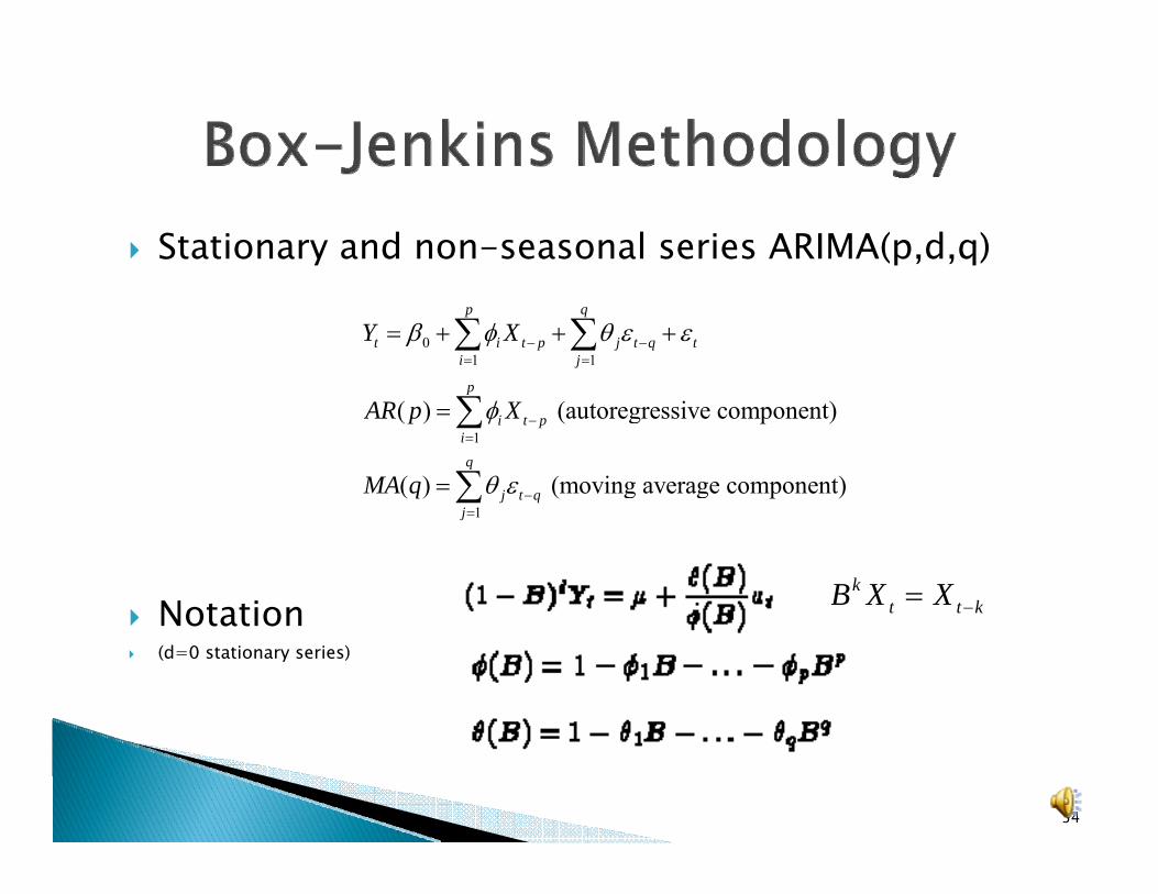
Stationary and non-seasonal series ARIMA(p,d,q)

Notation(d=0 stationary series)

34

01 1

1

1

( ) (autoregressive component)

( ) (moving average component)

p q

t i t p j t q ti j

p

i t pi

q

j t qj

Y X

AR p X

MA q

β φ θ ε ε

φ

θ ε

− −= =

−=

−=

= + + +

=

=

∑ ∑

∑

∑

kt t kB X X −=

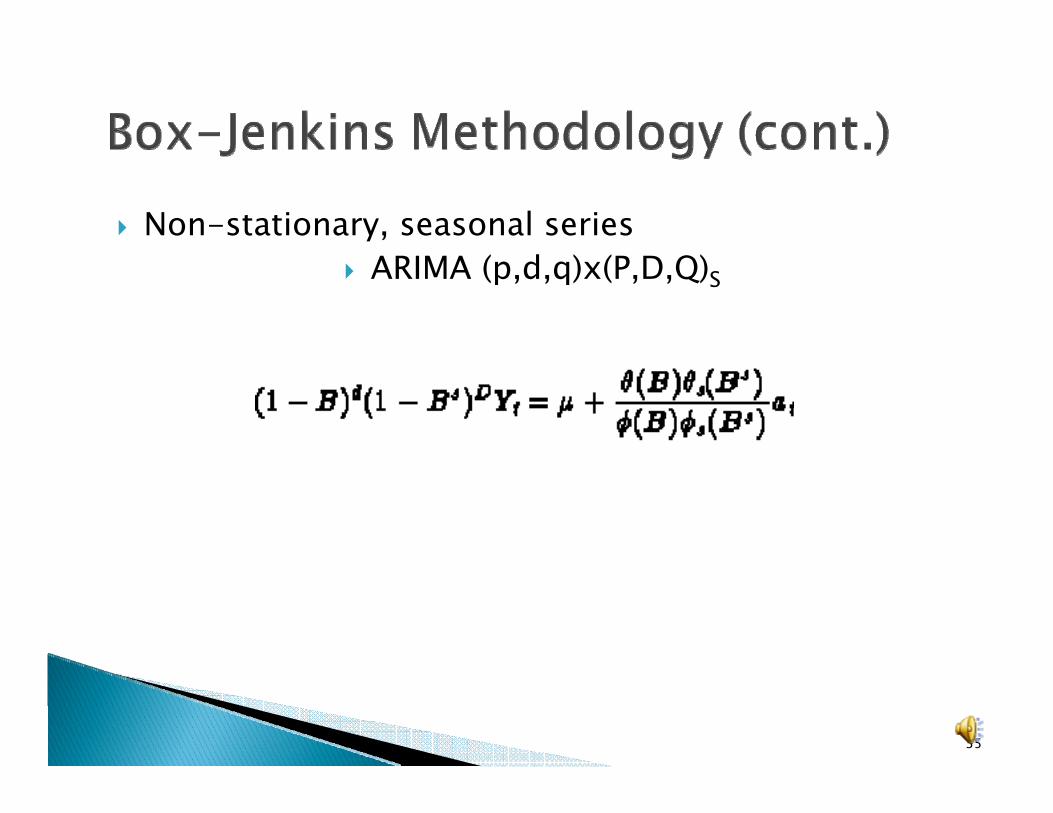
Non-stationary, seasonal series ARIMA (p,d,q)x(P,D,Q)S

35

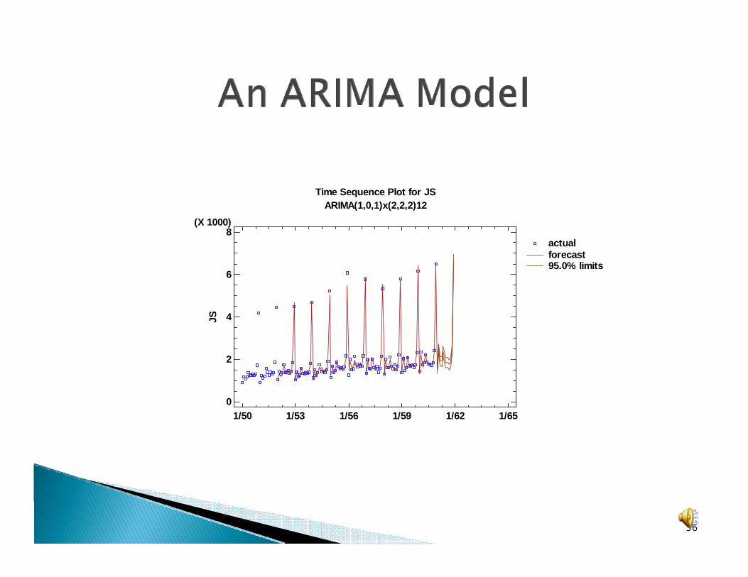
36

Time Sequence Plot for JSARIMA(1,0,1)x(2,2,2)12

1/50 1/53 1/56 1/59 1/62 1/650

2

4

6

8(X 1000)

JS

actualforecast95.0% limits

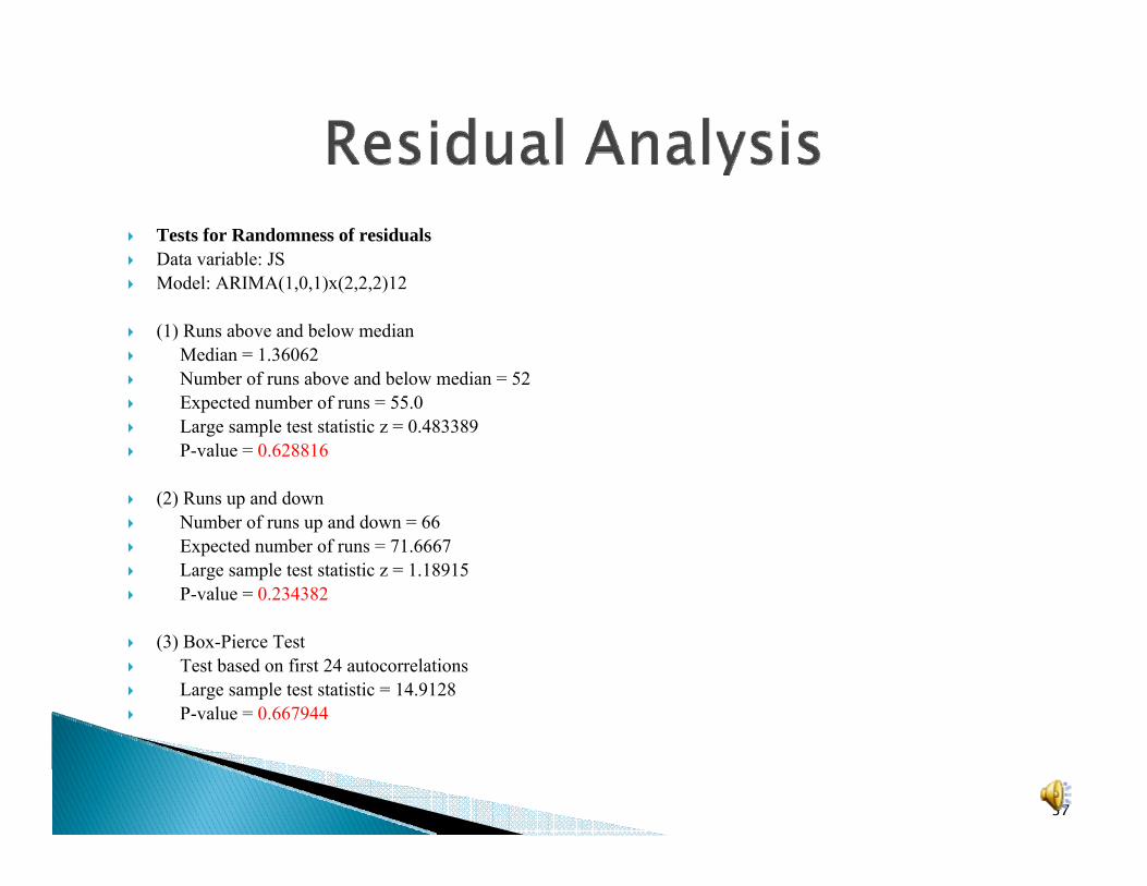
Tests for Randomness of residualsData variable: JSModel: ARIMA(1,0,1)x(2,2,2)12

(1) Runs above and below medianMedian = 1.36062Number of runs above and below median = 52Expected number of runs = 55.0Large sample test statistic z = 0.483389P-value = 0.628816

(2) Runs up and downNumber of runs up and down = 66Expected number of runs = 71.6667Large sample test statistic z = 1.18915P-value = 0.234382

(3) Box-Pierce TestTest based on first 24 autocorrelationsLarge sample test statistic = 14.9128P-value = 0.667944

37

38

39

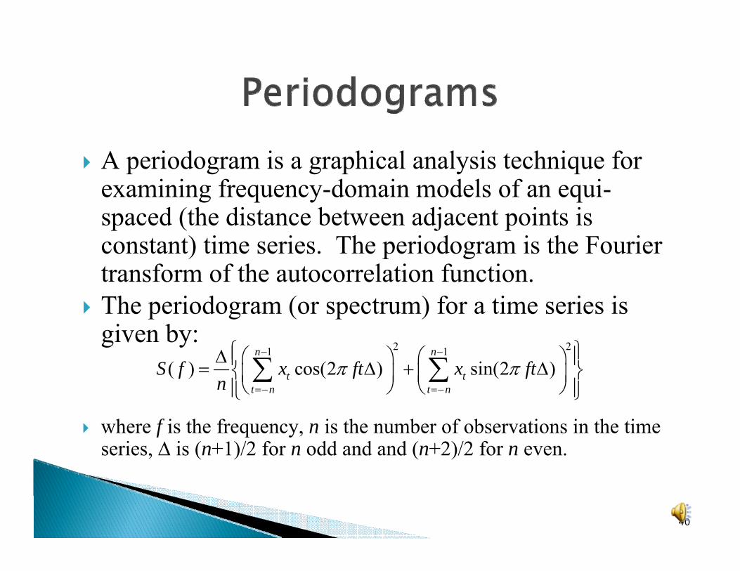
A periodogram is a graphical analysis technique for examining frequency-domain models of an equi-spaced (the distance between adjacent points is constant) time series. The periodogram is the Fourier transform of the autocorrelation function.The periodogram (or spectrum) for a time series is given by:

where f is the frequency, n is the number of observations in the time series, ∆ is (n+1)/2 for n odd and and (n+2)/2 for n even.

40

2 21 1

( ) cos(2 ) sin(2 )n n

t tt n t n

S f x ft x ftn

π π− −

=− =−

⎧ ⎫Δ ⎛ ⎞ ⎛ ⎞⎪ ⎪= Δ + Δ⎨ ⎬⎜ ⎟ ⎜ ⎟⎝ ⎠ ⎝ ⎠⎪ ⎪⎩ ⎭∑ ∑

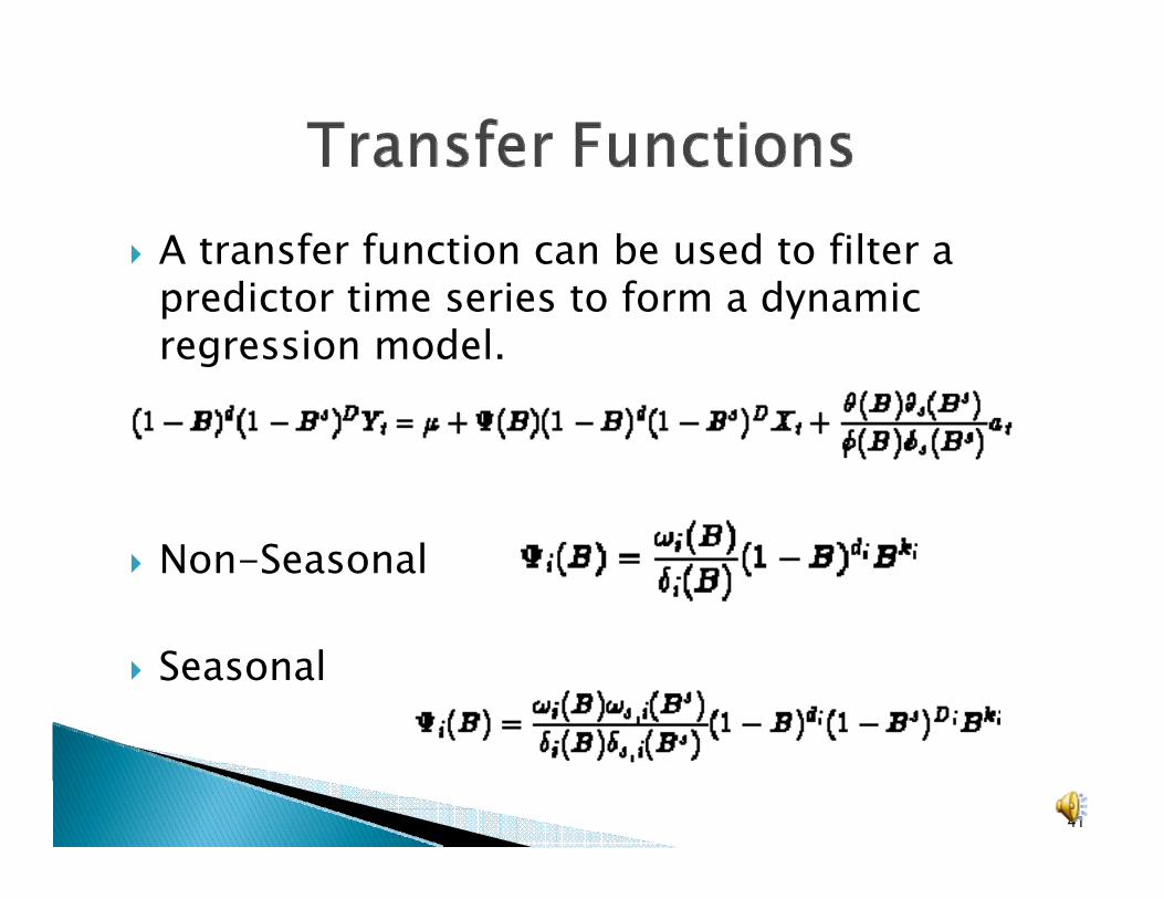
A transfer function can be used to filter a predictor time series to form a dynamic regression model.

Non-Seasonal

Seasonal

41

Surveys Delphi methodScenariosAnalogyAnalytic Hierarchy/Network Process (AHP/ANP)

42

A process developed in the 1970’s by T.L.SaatyBased of paired comparisons to develop relative measurement for single criteriaComposition of the single criteria scales can be:◦ Hierarchical (when no dependencies among the

criteria exist)◦ Network (when dependencies among the criteria are

allowed)

43

Saaty, T. L. (1980). The Analytic Hierarchy Process. New York, McGraw Hill.Saaty, T. L. (1986). "Axiomatic foundation of the Analytic Hierarchy Process." Management Science 32(7): 841-855.Saaty, T. L. (1994). Fundamentals of Decision Making. Pittsburgh, PA, RWS Publications.

44

Decomposition (Hierarchy or Network)Measurement (pairwise comparisons)Synthesis

45

From the paper

"Projecting the Average Family Size in Rural India by the Analytic Hierarchy Process,“ by T.L. Saaty and M. Wong. Journal of Mathematical Sociology, Vol. 9, 1983, pp. 181-209.

46

A1: cultureA2: economic developmentA3: land fragmentationA4: declining infant mortalityA5: high availability of contraceptionA6: scarcity of resources

47

The Consistent Case

48

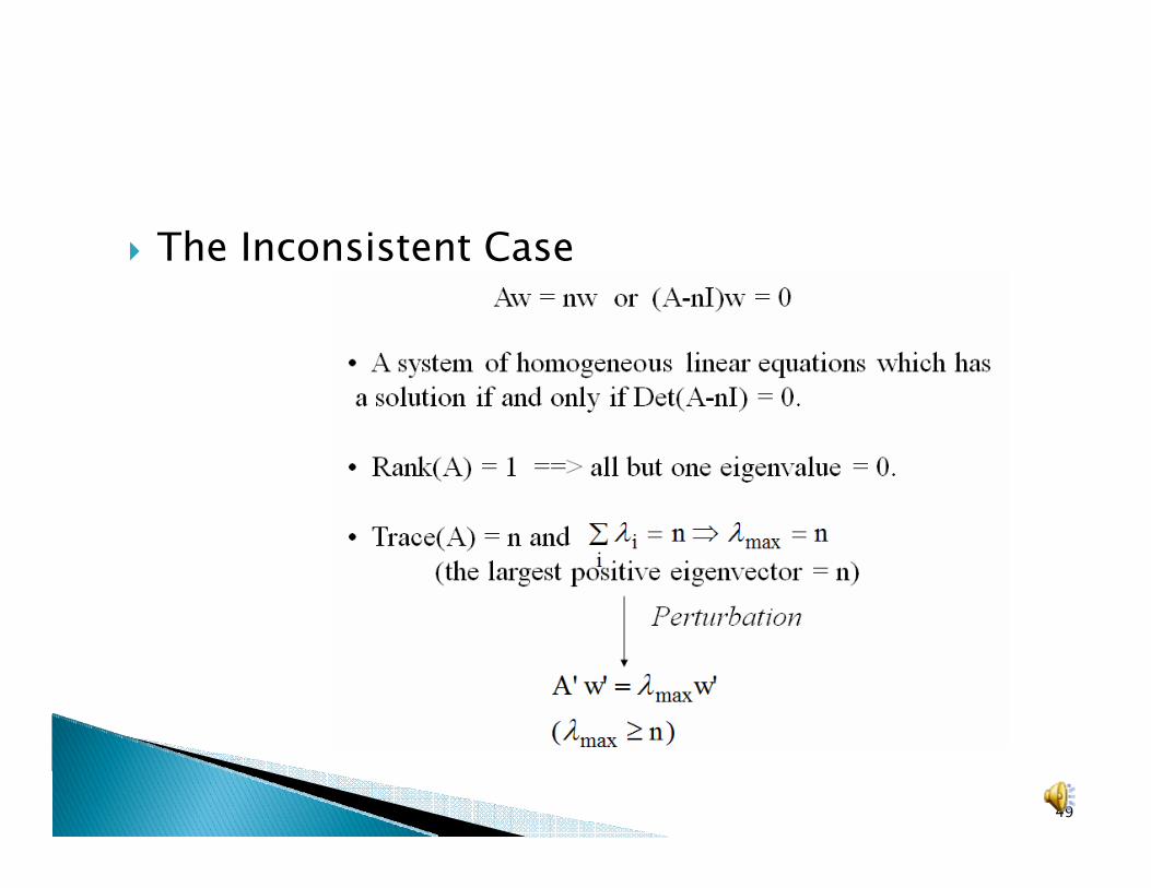
The Inconsistent Case

49

50

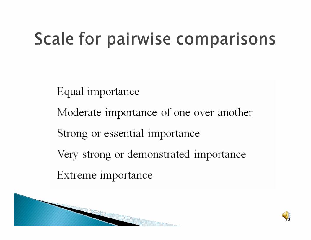
1 Equal importance3 Moderate importance5 Strong or essential importance7 Very strong or demonstrated9 Extreme importance2,4,6,8 Intermediate valuesUse Reciprocals for Inverse Comparisons

51

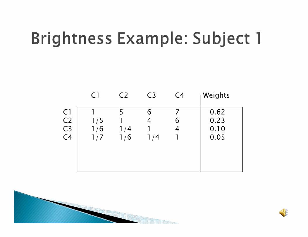
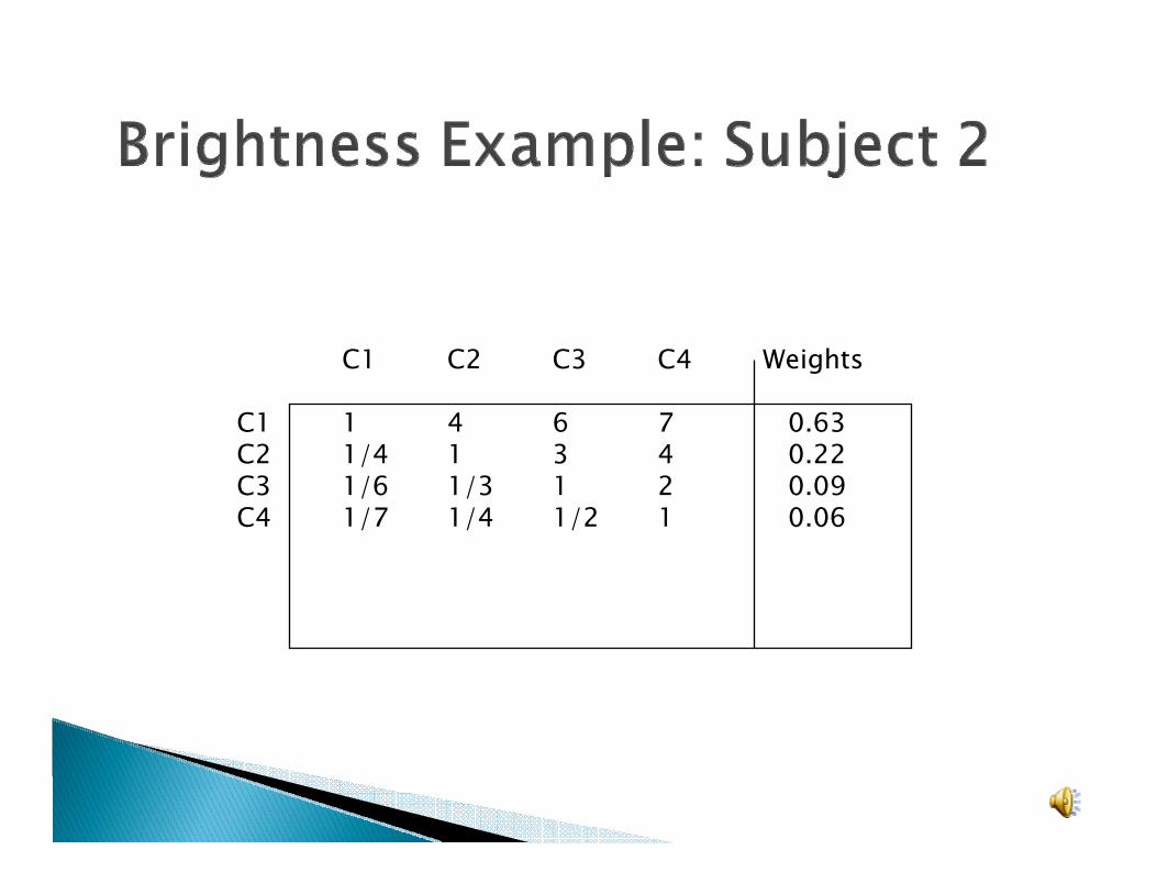
Chairs DistanceC1 9C2 15C3 21C4 28

C1 C2 C3 C4 Weights

C1 1 5 6 7 0.62C2 1/5 1 4 6 0.23C3 1/6 1/4 1 4 0.10C4 1/7 1/6 1/4 1 0.05

C1 C2 C3 C4 Weights

C1 1 4 6 7 0.63C2 1/4 1 3 4 0.22C3 1/6 1/3 1 2 0.09C4 1/7 1/4 1/2 1 0.06

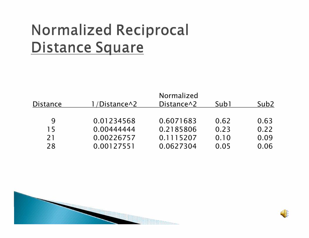
NormalizedDistance 1/Distance^2 Distance^2 Sub1 Sub2

9 0.01234568 0.6071683 0.62 0.6315 0.00444444 0.2185806 0.23 0.2221 0.00226757 0.1115207 0.10 0.0928 0.00127551 0.0627304 0.05 0.06

Comparison of Intangibles

The same procedure as we use for distancecan be used to compare things with intangible properties. For example, we could compare apples according to:

• TASTE• AROMA• RIPENESS

Contribution Relativeto Family Size Priority

AlA2 A3 A4 A5 A6 Weights

Al 1 1/71/3 1/5 1/9 1/8 .025A2 7 1 3 2 1/5 1/3 .128A3 3 1/31 1/5 1/5 1/5 .053A4 5 1/23 1 1/5 1/3 .096A5 9 5 5 5 1 4 .467A6 8 3 5 3 1/4 1 .231

λmax= 6.431C.I. = 0.086

A1: cultureA2: economic developmentA3: land fragmentationA4: declining infant mortalityA5: high availability of contraceptionA6: scarcity of resources

Economic Development Relative Priority A2 1 2 3 Weights 1 1 2 3 .025 2 1/2 1 2 .297 3 1/3 1/2 1 .163 λmax = 3.009 C.I. = 0.005

Declining Infant Mortality Relative Priority A4 1 2 3 Weights 1 1 1/3 1/2 .169 2 3 1 1 .443 3 2 1 1 .387 λmax = 3.018 C.I. = 0.009

High Availability of Contraception Relative Priority A5 1 2 3 Weights 1 1 1/3 1/2 .163 2 3 1 2 .540 3 2 1/2 1 .297 λmax = 3.009 C.I. = 0.005

Scarcity of Resources Relative Priority A6 1 2 3 Weights 1 1 1/4 1/2 .149 2 4 1 1/2 .376 3 2 2 1 .474 λmax = 3.217 C.I. = 0.109

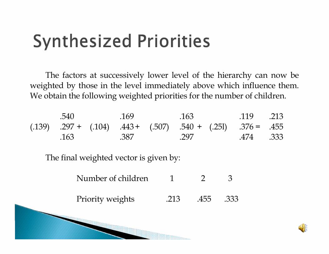
The factors at successively lower level of the hierarchy can now beweighted by those in the level immediately above which influence them.We obtain the following weighted priorities for the number of children. .540 .169 .163 .119 .213 (.139) .297 + (.104) .443 + (.507) .540 + (.25l) .376 = .455 .163 .387 .297 .474 .333 The final weighted vector is given by: Number of children 1 2 3 Priority weights .213 .455 .333

Finally we compute the expected number of children for a family in rural India as our expected value: (.213 x 1) + (.455 x 2) + (.333 x 3) = 2.122.

A large number of thriving children is still highly desired by the majority of rural Indian families. One of the most common explanations of high fertility is the alleged preference of Indian parents for male children. Sons are a man's best support when he needs help most, during harvests or in confrontations in village fights and feuds. It is also believed that sons can improve the parents destiny in the afterworld by performing certain rites after the parents' deaths.

Our purpose now is to use the foregoing factors as determinants of the average number of children in a family in rural India:

Level I: Optimal family size

Level II: Al CultureA2 Economic factorsA3 Demographic factorsA4 Availability of

contraceptives

Level III:◦ Bl Religion◦ B2Women's status◦ B3 Manlihood◦ B4 Cost of child-rearing◦ B5Old age security◦ B6Labor◦ B7 Economic improvement◦ B8Prestige and strength◦ B9 Short life expectancy◦ Bl0 High infant mortality◦ B11 High level of availability of contraception◦ B12 Medium level of availability of contraception◦ B13 Low level of availability of contraception

.073 .028 .039 .061 .092 .051 .117 .057 .088 .102 .147 .099 .298 .141 .184 .190 .269 .205 (.243) .303 + (.370) .269 + (.183) .282 + (.097) .301 + (.107) .224 = .279 .096 .259 .204 .181 .128 .188 .050 .161 .130 .110 .085 .116 .033 .086 .037 .054 .054 .064 Thus, the relative priority weights of the number of children are asfollows: Number of children 4 5 6 7 8 9 10 Weights .051 .099 .205 .279 .188 .116 .064

The weights obtained for each number of children under each factor at level III are finally multiplied and summed. We have

(4x.051) + (5x.099) + (6x.205) + (7x.279) + (8x.188) + (9x.116) + (lOx.064) = 6.494.

It has been reported by many that the mean number of children a women has after she completes her reproductive cycle is 6.4. (Driver 1963: 86, 101-102; Ridker 1969: 280-281; Mandelbaum 1974: 15).

Total Fertility Rate (average number of children born to a woman during her lifetime) 3.30 Only nine states or union territories in the country have a TFR less than or equal to the desired 2.1: Eleven have a total fertility rate of more than 2.1but less than 3.0. At least 12 have a total fertility rate of 3.0 or over. Eighteen per cent of births are to teenage women aged between 15 and 19Forty-nine per cent of women give birth for the first time by age 20.The average age at first marriage (or informal union) is 20. Forty-three per cent of married women are using modern methods of contraception. Females in secondary school/100 males: 65

68

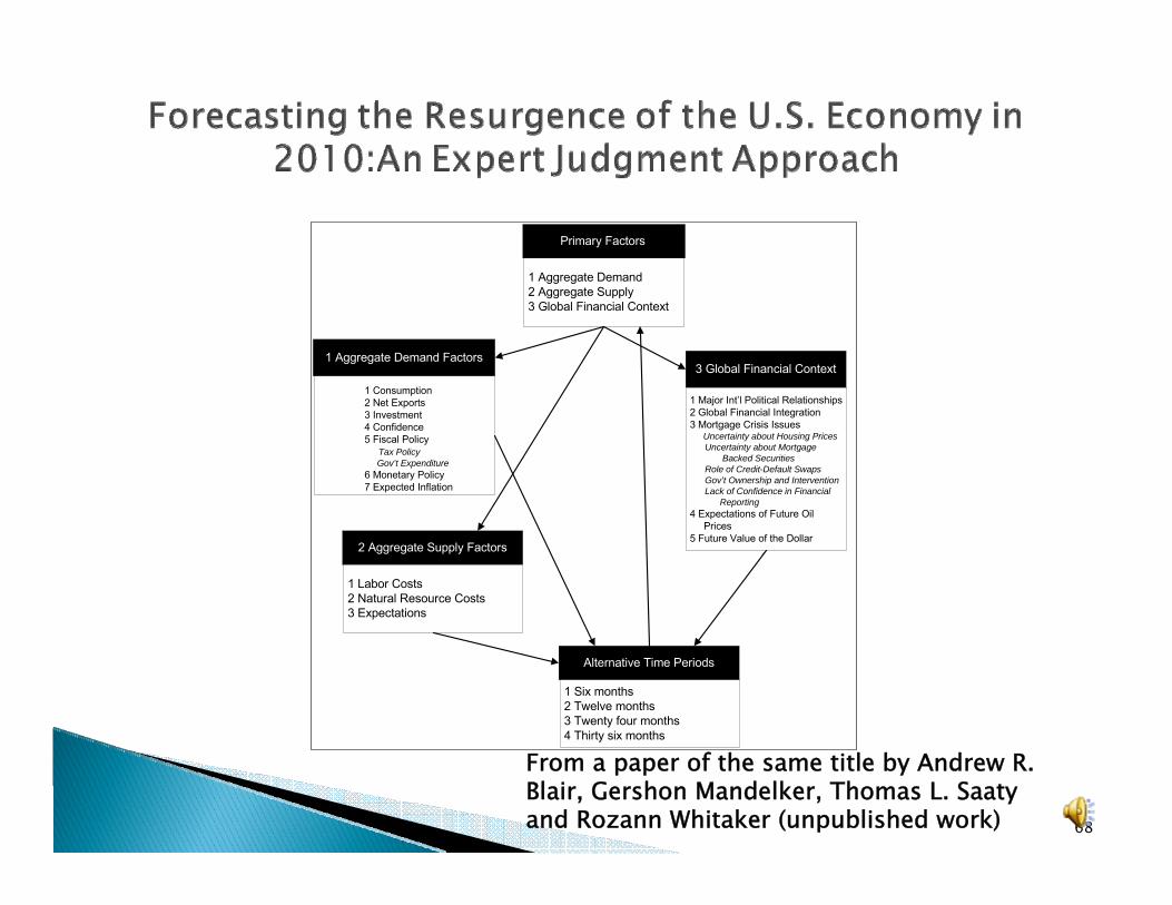
3 Global Financial Context

1 Major Int’l Political Relationships2 Global Financial Integration3 Mortgage Crisis Issues Uncertainty about Housing Prices

Uncertainty about MortgageBacked Securities

Role of Credit-Default SwapsGov’t Ownership and InterventionLack of Confidence in Financial

Reporting4 Expectations of Future Oil Prices5 Future Value of the Dollar

Primary Factors

1 Aggregate Demand2 Aggregate Supply3 Global Financial Context

1 Aggregate Demand Factors

1 Consumption2 Net Exports3 Investment4 Confidence5 Fiscal Policy Tax Policy

Gov’t Expenditure6 Monetary Policy7 Expected Inflation

2 Aggregate Supply Factors

1 Labor Costs2 Natural Resource Costs3 Expectations

Alternative Time Periods

1 Six months2 Twelve months3 Twenty four months4 Thirty six months

From a paper of the same title by Andrew R. Blair, Gershon Mandelker, Thomas L. Saaty and Rozann Whitaker (unpublished work)

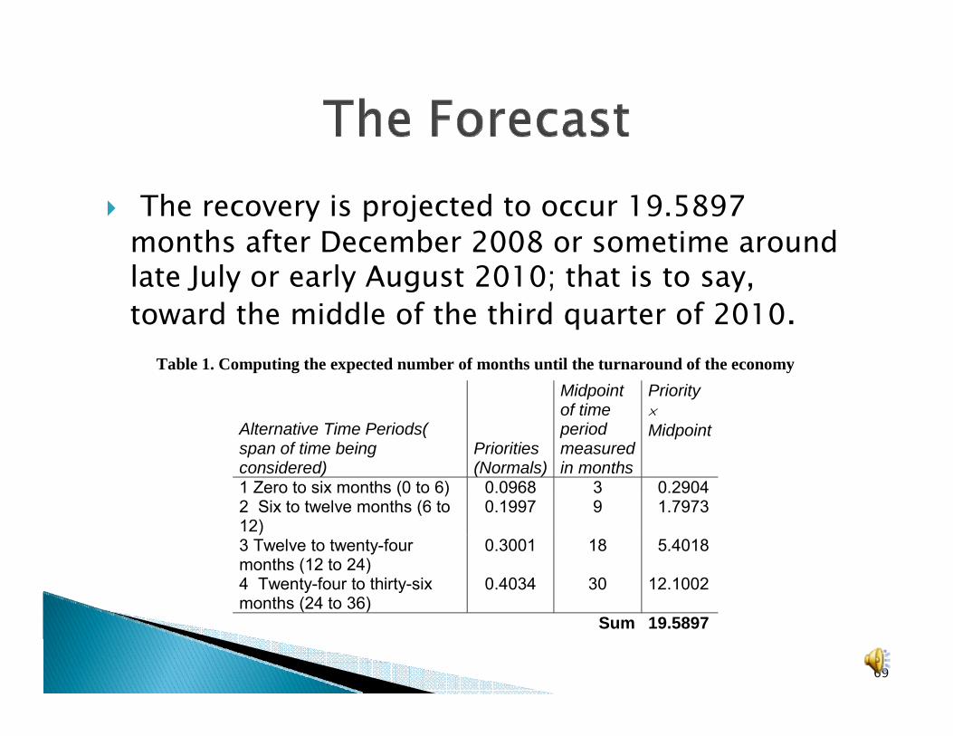
The recovery is projected to occur 19.5897 months after December 2008 or sometime around late July or early August 2010; that is to say, toward the middle of the third quarter of 2010.

69

Table 1. Computing the expected number of months until the turnaround of the economy

Alternative Time Periods( span of time being considered)

Priorities (Normals)

Midpoint of time period measured in months

Priority × Midpoint

1 Zero to six months (0 to 6) 0.0968 3 0.29042 Six to twelve months (6 to 12)

0.1997 9 1.7973

3 Twelve to twenty-four months (12 to 24)

0.3001 18 5.4018

4 Twenty-four to thirty-six months (24 to 36)

0.4034 30 12.1002

Sum 19.5897

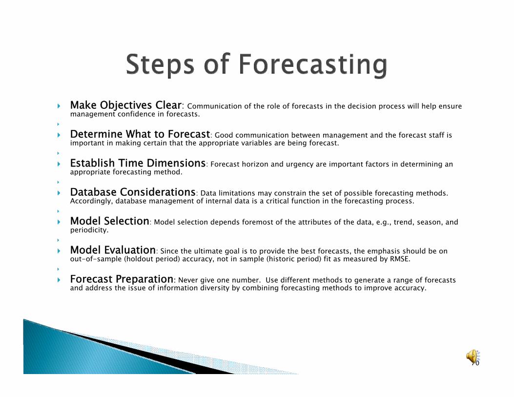
Make Objectives Clear: Communication of the role of forecasts in the decision process will help ensure management confidence in forecasts.

Determine What to Forecast: Good communication between management and the forecast staff is important in making certain that the appropriate variables are being forecast.

Establish Time Dimensions: Forecast horizon and urgency are important factors in determining an appropriate forecasting method.

Database Considerations: Data limitations may constrain the set of possible forecasting methods. Accordingly, database management of internal data is a critical function in the forecasting process.

Model Selection: Model selection depends foremost of the attributes of the data, e.g., trend, season, and periodicity.

Model Evaluation: Since the ultimate goal is to provide the best forecasts, the emphasis should be on out-of-sample (holdout period) accuracy, not in sample (historic period) fit as measured by RMSE.

Forecast Preparation: Never give one number. Use different methods to generate a range of forecasts and address the issue of information diversity by combining forecasting methods to improve accuracy.

70