OW V J AA center of excellence in earth sciences and engineering

A Division of Southwest Research Institute" 6220 Culebra Road • San Antonio, Texas, U.S.A. 78228-5166 (210) 522-5160 • Fax (210) 522-5155

January 22, 2001 Contract No. NRC-02-97-009 Account No. 20.01402.861

20.01402.471 U.S. Nuclear Regulatory Commission ATTN: Mrs. Deborah A. DeMarco Two White Flint North 11545 Rockville Pike Mail Stop T8A23 Washington, DC 20555

Subject: Programmatic Review of Book Chapter

Dear Mrs. DeMarco:

The enclosed draft for a book chapter is being submitted for programmatic review. The title of the chapter is "Statistical characterization of spatial variability in sedimentary rock." This manuscript is intended to be included in a book titled "Small Scale Crustal Heterogeneity."

Please advise me of the results of your programmatic review. Your cooperation in this matter is appreciated.

Sincerely,

Budhi Sagar Technical Director

/ph Enclosures cc: J. Linehan T. Essig W. Patrick

E. Whitt K. Stablein CNWRA Directors B. Meehan N. Coleman CNWRA Element Mgrs J. Greeves B. Leslie T. Nagy (SwRI Contracts) J. Holonich P. Justus P. Maldonado W. Reamer

Washington Office * Twinbrook Metro Plaza #210 12300 Twinbrook Parkway ° Rockville, Maryland 20852-1606

Chapter 11

Statistical characterization of spatial variability in sedimentary rock

Scott Painter Center for Nuclear Waste Regulatory Analyses; Southwest Research Institute; Culebra Rd.; San

Antonio Texas; 78250

1. INTRODUCTION

Spatial variability is a ubiquitous feature of sedimentary rock. The

physical properties of sedimentary formations are not smoothly varying

functions of position, but are subject to abrupt changes of various magnitudes. These abrupt contrasts in rock properties affect the propagation

and dispersion of seismic energy, with important implications for

geophysical studies. Spatial heterogeneity is also a dominant control on fluid and contaminant movement, thereby affecting the dynamics of groundwater aquifers and petroleum reservoir.

The traditional view of heterogeneity in sedimentary rock is of idealized layers with constant properties within each layer. This view is not consistent with outcrop studies or borehole geophysical data, which typically show

complex and erratic fluctuations on a variety of spatial scales. Motivated by

the need to improve petroleum reservoir production forecasts, contaminant transport predictions, and seismic deconvolution/inversion methods, a number of researchers have constructed stochastic models of spatial variability in sedimentary rock. These modeling efforts have as a common

element the abandonment of the familiar random process models based on

I

the Gaussian distribution and a finite correlation scale, and use instead distributions other than the Gaussian, and/or multiple-scale fractal-like correlation models. This chapter summarizes various efforts to construct such non-classical models and compares the success of several approaches using several example datasets.

2. REPRODUCIBLE STATISTICAL FEATURES OF

SEDIMENTARY ROCK

2.1 Non-Gaussian distribution of property fluctuations

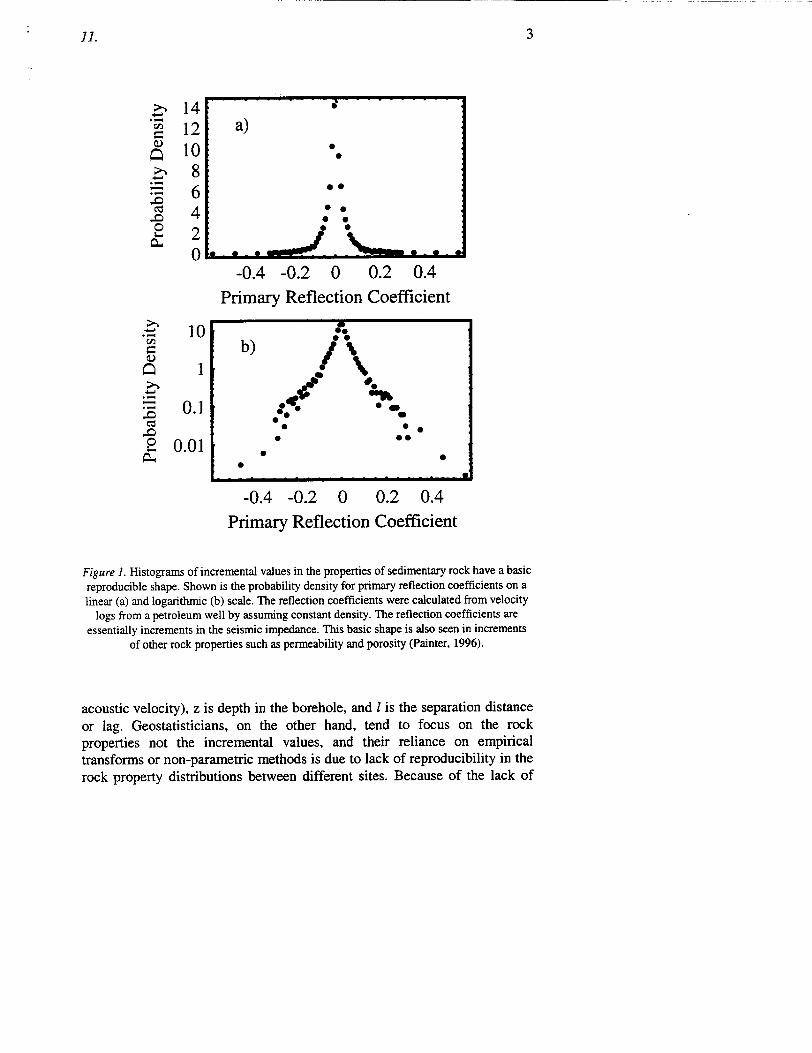
Exploration geophysicists were among the first to identify reproducible statistical features in the physical properties of sedimentary rock. Specifically, it has been known for some time that the probability densities for primary seismic reflection coefficients have a basic reproducible shape (Agard, 1961; O'Doherty and Anstey, 1971; Walden and Hosken, 1986). An example constructed from a borehole log of seismic velocity is shown in Figure 1. The velocity log is from the Goodwyn 1 well (located on the northwest shelf of Australia), which spans a long sequence of platform carbonates and marine clastics. Variations in formation density were neglected in constructing the reflection coefficients. The basic shape for the reflection coefficient probability density is "bell shaped" (concave downward in the center switching to concave upward in the tails), but is more peaked than the Gaussian (leptokurtic). When plotted on a logarithmic scale (Figure lb), it is also apparent that the tails of the density are enhanced by orders of magnitude over the Gaussian distribution (Painter et al. 1995).

This identification of reproducible statistical features is in striking contrast to the conventional practice in petroleum and groundwater geostatistics, which rely heavily on empirical transforms and non-parametric methods to honor formation-specific statistical features. This difference in approach can be understood by noting that geophysicists focus naturally on the increments or contrasts in properties rather the properties themselves. Specifically, the reflection coefficient sequence R(z) can be written as increments R(z)=W(z+l)-W(z) when the impedance contrasts are small. Here W(z)=1/2 Log[ I(z)], I(z) is the seismic impedance (product of rock density and

Chapter I1I2

11.

°0,,

0"

CIO

0D

14 12 10 8 6 4 2 0

10

I

0.1

0.01

a)

• ,,

-0.4 -0.2 0 0.2 0.4 Primary Reflection Coefficient

-0.4 -0.2 0 0.2 0.4Primary Reflection Coefficient

Figure 1. Histograms of incremental values in the properties of sedimentary rock have a basic reproducible shape. Shown is the probability density for primary reflection coefficients on a linear (a) and logarithmic (b) scale. The reflection coefficients were calculated from velocity

logs from a petroleum well by assuming constant density. The reflection coefficients are essentially increments in the seismic impedance. This basic shape is also seen in increments

of other rock properties such as permeability and porosity (Painter, 1996).

acoustic velocity), z is depth in the borehole, and I is the separation distance or lag. Geostatisticians, on the other hand, tend to focus on the rock properties not the incremental values, and their reliance on empirical transforms or non-parametric methods is due to lack of reproducibility in the rock property distributions between different sites. Because of the lack of

O*

b)

-lb.

0' em

*5 U *

* 00

5 0 0

3

reproducibility in the rock property distribution compared with the reproducibility in the increment distribution, it has been suggested (Painter, 1995) that it is more appropriate to model the properties of sedimentary rock as non-stationary with stationary increments. This approach is similar to relaxing the second-order stationarity hypothesis in favor of the intrinsic hypothesis (see e.g. Journel and Huijbregts, 1978), a generalization that is

rarely applied in practice. Stationarity in the increments is a weaker condition than stationarity in the rock properties; the latter implies the

former, but the converse is not true. Such stationary increment models are sometimes referred to as random motion models, by analogy with the classical Brownian motion.

The reproducible shape of the reflection coefficient probability density is also shared by increments in other physical properties measured in

sedimentary formations. This behavior has been observed in sonic velocity, density, and porosity logs from deep petroleum wells (Painter and Paterson, 1994; Painter, 1995), in outcrop and core-based measurements of permeability (Painter, 1996, 2001) and in in-situ flow-meter measurements of permeability (Liu and Molz, 1997a). The basic shape for the distribution has been observed in both the horizontal and the vertical directions. The width of the increment distribution is typically smaller in the horizontal direction, reflecting reduced variability in the horizontal direction.

The reproducible shape of the increment distribution is simply the manifestation of stratification. As we move from one point in the formation to the next, there is a large probability that the observed rock property will change little. These abundant small changes produce the large peak near zero. However, there is a small but non-negligible probability of finding an abrupt change that might, for example, be associated with changes in rock type or strata boundaries. These infrequent large changes in rock properties produce the slowly decaying tails in the distribution on increments.

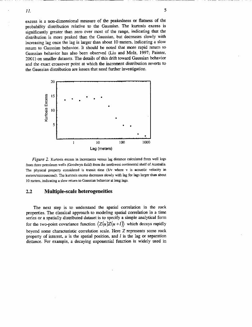
Most of the previous studies of the distributions of incremental values focused on increments defined on lag or separation distances in the range of a few centimeters to a few meters. Results for longer lag distances are more limited, but the available evidence suggests that the increment histogram retains the same basic shape but drifts slowly toward the Gaussian as the lag increases (Liu and Molz, 1997a; Painter, 2001). An example of this is shown in Figure 2. In constructing this plot, increments in transit time (1/v where v is velocity in meters/microseconds) defined on various lags were analyzed for the kurtosis excess. The data comes from the Goodwyn 1, 8 and 9 wells on the northwest shelf of Australia (18939 measurements). The kurtosis

Chapter I114

11. 5

excess is a non-dimensional measure of the peakedness or flatness of the probability distribution relative to the Gaussian. The kurtosis excess is

significantly greater than zero over most of the range, indicating that the distribution is more peaked than the Gaussian, but decreases slowly with increasing lag once the lag is larger than about 10 meters, indicating a slow return to Gaussian behavior. It should be noted that more rapid return to Gaussian behavior has also been observed (Liu and Molz, 1997; Painter, 2001) on smaller datasets. The details of this drift toward Gaussian behavior and the exact crossover point at which the increment distribution reverts to the Gaussian distribution are issues that need further investigation.

20

¢ 15 o x

* • 10

5

1 10 100 1000

Lag (meters)

Figure 2. Kurtosis excess in increments versus lag distance calculated from well logs

from three petroleum wells (Goodwyn field) from the northwest continental shelf of Australia.

The physical property considered is transit time (1/v where v is acoustic velocity in

meters/microsecond). The kurtosis excess decreases slowly with lag for lags larger than about

10 meters, indicating a slow return to Gaussian behavior at long lags.

2.2 Multiple-scale heterogeneities

The next step is to understand the spatial correlation in the rock properties. The classical approach to modeling spatial correlation in a time series or a spatially distributed dataset is to specify a simple analytical form

for the two-point covariance function (Z(u)Z(u + 1)) which decays rapidly

beyond some characteristic correlation scale. Here Z represents some rock property of interest, u is the spatial position, and I is the lag or separation distance. For example, a decaying exponential function is widely used in

groundwater hydrology to model spatial correlation in Y=log K, where K is the hydraulic conductivity. Within the exponential model, the characteristic decay length for the exponential function defines a characteristic length scale for the fluctuations. Experimental detection of the spatial correlation is often accomplished by considering estimators for the variogram

function ([Z(u)- Z(u + l)]2), which is closely related to the two-point

covariance if the sequence is stationary.

A large number of studies have produced clear evidence to contradict the notion of a characteristic correlation length in sedimentary rock. For example, meta-analyses of field data from groundwater aquifers have shown that hydraulic conductivity and dispersivities tend to increase with increasing scale (see, for example, Neuman (1990,1994)). Specifically, hydraulic conductivities tend to increase, on average, with increasing scale of support and apparent dispersivities tend to increase with increasing travel distance over a wide range. Moreover, the apparent correlation scale in the logarithm of hydraulic conductivity increases nearly linearly with the size of the data window (Gelhar, 1993). Although not specifically addressing the physical properties of sedimentary rock, the variances of gold grades have been reported (Krige, 1970) to increase with increasing area of investigation (see also Journel (1978)). Taken together, these observed dependencies on the spatial scale of support are inconsistent with a single scale for the spatial correlation and consistent with the intuitive notion that spatial fluctuations in rock properties occur over a wide range of scales. In other words, the trends are consistent with the concept of long-range or fractal correlation in the rock properties.

Several authors provide direct evidence for long-range spatial correlation in sedimentary rock (Walden and Hosken, 1985; Hewett, 1986; Todoeschuck and Jensen 1988; Pilkington and Todoeschuck, 1990; Goggin et al., 1992; Molz and Boman, 1993; Painter and Paterson, 1994; Painter et al., 1995; Painter, 1995,1996). These studies consider a range of physical measurements and typically rely on one of three measures of spatial correlation: the variogram (or closely related measures of width of the increment distribution), the Fourier spectrum, or the R/S statistic (Mandelbrot, 1969). Each of these methods can detect a characteristic scale length; a power-law dependence on lag (or wavenumber in the case of spectral analysis) is the signature for scale-invariant or fractal behavior. Despite the differences in analysis techniques and measurement types, these studies all reach similar conclusions: that the physical properties of sedimentary rock are not consistent with the classical notion of characteristic correlation scale.

Chapter 116

11.

Walden and Hosken (1985) and Todoeschuck and Jensen (1988) showed that primary reflection coefficients constructed from borehole geophysical

measurements have a Fourier spectrum resembling a power law. Given that

the reflection coefficients are essentially increments in the seismic

impedance, this result is consistent with a random fractal motion model for

the seismic impedance. Pilkington and Todoeschuck (1990) show that the

spectra for several geophysical logs (density, resistivity, natural gamma-ray,

neutron density) in several wells spanning sedimentary sequences are also

well approximated as power-law.

Hewett (1986) used the R/S analysis technique, variogram analyses, and

spectral analyses to conclude that porosity measured by geophysical methods in nearly vertical boreholes have long-range spatial correlation. Molz and

Boman (1993) took a similar approach, and considered spatial correlation in hydraulic conductivity, as did Goggin et al. (1992) who analyzed permeability measured on outcrops. All of these studies reached a similar conclusion about long-range spatial correlation. These studies considered the

porosity or permeability to be the stationary increments in a random motion process.

Painter and Paterson (1994), Painter et al. (1995), and Painter (1995b)

follow a line of investigation similar to that of Walden and Hosken (1985)

and consider several well logs (porosity, velocity, density, and resistivity) as

random motions (non-stationary random processes with stationary increments). They considered a robust variant on the variogram - the first

order structure function - and showed that it was accurately fitted by a

power-law function over a wide range of spatial scales. Painter (1996) showed that the same scaling occurs in core-based and outcrop-based measurements of permeability in sedimentary formations.

7

Chapter 11

50 E Goodwyn wells

ca20

. 10

2

1 10 100 1000 Separation Distance (meters)

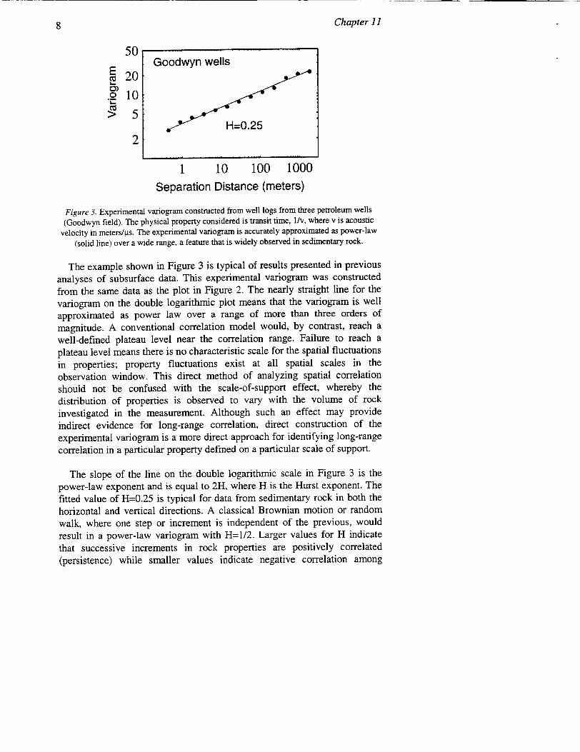
Figure 3. Experimental variogram constructed from well logs from three petroleum wells

(Goodwyn field). The physical property considered is transit time, lIv, where v is acoustic

velocity in meters/pAs. The experimental variogram is accurately approximated as power-law

(solid line) over a wide range, a feature that is widely observed in sedimentary rock.

The example shown in Figure 3 is typical of results presented in previous analyses of subsurface data. This experimental variogram was constructed

from the same data as the plot in Figure 2. The nearly straight line for the variogram on the double logarithmic plot means that the variogram is well approximated as power law over a range of more than three orders of

magnitude. A conventional correlation model would, by contrast, reach a

well-defined plateau level near the correlation range. Failure to reach a plateau level means there is no characteristic scale for the spatial fluctuations in properties; property fluctuations exist at all spatial scales in the

observation window. This direct method of analyzing spatial correlation should not be confused with the scale-of-support effect, whereby the distribution of properties is observed to vary with the volume of rock investigated in the measurement. Although such an effect may provide indirect evidence for long-range correlation, direct construction of the

experimental variogram is a more direct approach for identifying long-range correlation in a particular property defined on a particular scale of support.

The slope of the line on the double logarithmic scale in Figure 3 is the power-law exponent and is equal to 2H, where H is the Hurst exponent. The fitted value of H=0.25 is typical for data from sedimentary rock in both the horizontal and vertical directions. A classical Brownian motion or random walk, where one step or increment is independent of the previous, would

result in a power-law variogram with H=1/2. Larger values for H indicate that successive increments in rock properties are positively correlated (persistence) while smaller values indicate negative correlation among

8

successive increments (anti-persistence). Anti-persistence means that a positive change in properties is followed, on average, by a negative change

and vice-versa. Anti-persistence is the general situation for sedimentary

rock, and is simply a manifestation of the tendency to switch back and forth

- after a random duration - between two different rock types (i.e. alternating sequences of sand and shale).

3. STATISTICAL MODELS FOR SPATIAL VARIABILITY

Most of the previous effort on the statistical properties of sedimentary

rock has focused on characterization only, i.e. on the identification of simple

reproducible features; comparatively little effort has been devoted to

developing well defined statistical models that capture these features.

3.1 Models for the increment distribution

Walden and Hosken (1986) considered models for the amplitude

distributions for primary reflection coefficients. Because the primary

reflection coefficients can be considered as increments in the seismic impedance, this work represents an important early effort at understanding property variations in a more general context. In the following the symbol A

is used to represent increments in some rock property Z; if we associate the

logarithm of seismic impedance with Z, then A represents seismic reflection coefficients.

Walden and Hosken (1998) proposed two statistical distributions to

capture the observed shape of the amplitude distribution for reflection coefficient: a mixture of two Laplace (or two-sided exponential) distributions, and a generalized Gaussian distribution. The probability density for increments in the Laplace-mixture model is

f (A; P,,ý"1"2 ) = -1- ex -_IA[ l+ - p ex --•2,, 'A'

fp'/pý 2A2AA

where X• and X2 are scale parameters for the first and second populations, respectively, and p is a mixing parameter that defines the relative proportions of the two populations. Walden and Hosken provide a maximum likelihood estimator for the parameters, compare the fit to several reflection

coefficient sequences, and discuss the interpretations from the perspective of sedimentary geology.

911.

Chapter 11

The generalized Gaussian distribution considered by Walden and Hosken

(1986) has probability density given by

a[ f(A;a,b) = 2bF(l /a)

where F is the gamma function, a is a shape parameter that runs between 0

(exclusive) and 2 (inclusive), and b is a positive real number that defines the

scale. When a=2, the generalized Gaussian reduces to the Gaussian. For a>2,

the density for the generalized Gaussian is more peaked than the Gaussian

and has more slowly decaying tails. When a>1, the density has a cusp at the

origin. Walden and Hosken also discuss how the two models - the Laplace

mixture and the generalized Gaussian - can be constructed from an infinite

mixture of Gaussian distributions.

A model for the distribution of seismic reflection coefficients and, more

generally, increments in rock properties was also considered by Painter and

colleagues (Painter and Paterson, 1994; Painter et al., 1995; Painter,

1995,1996). This work relied on the family of probability distribution known

as stable or Levy-stable distributions (Levy, 1936; Feller, 1972; Zolatarev,

1986). This family of distributions generalizes the Gaussian distribution and

has an important role in mathematical statistics as the limit distributions for

sums of certain independent random variables. If the variance of the

summand variables is finite, then the distribution of the sum will tend to the

Gaussian distribution, according to the central limit theorem. If the summand

variables have a distribution that is asymptotically power-law, then the

distribution of the sum will tend to one of the non-Gaussian members of the

stable distribution (generalized central limit theorem). Painter and colleagues

used the symmetric non-Gaussian Levy-stable distributions as models for

increments in rock properties. The probability density for these distributions does not have a closed form; the distribution is most easily defined through the characteristic function, which is the Fourier transform of the probability density. For the symmetric (about 0) stable distributions, the characteristic function is given by

f(v;a, C) = exp[- (cv' )a''

10

where C is a scale parameter and a e (0,2] is a shape parameter that

measures the deviation from Gaussianity. Probability densities can be obtained from the characteristic function by inverse Fourier transform. The

situation ot=2 represents the Gaussian distribution. As cc decreases from 2,

the probability density becomes more and more peaked at the origin with a slowly decaying power-law tail.

More recently, Painter (2001) proposed a new model for the increment

distribution that is based on subordination. Subordination is the process of

constructing a new random process by randomizing the variance in an

existing process (see e.g. Feller (1971)). In the subordination model, the

increment distribution is modeled as an infinite mixture of Gaussian

distributions with different variances

f (A)= fw(a)g (A; 0, a~do 0

where g is the Gaussian distribution with mean 0 and variance a, and the

function w represents a weighting function or distribution for standard

deviations. By choice of the subordinator w, considerable flexibility exists to

tune the shape of the increment distribution. By selecting w to be a dirac

delta function, the model reverts to a classical Gaussian based model. At the

other extreme, by selecting w as a function that is asymptotically power law,

the stable distribution is recovered. An intermediate degree of variability can

be modeled by selecting the subordinator to be a skewed distribution that is

more rapidly decaying than the power law. For example, Painter used a log

normal subordinator and showed that this was able to reproduce increment

distributions in Log K, where K is hydraulic conductivity. Within this

model, the increment distribution is given by

f(A) = (c; a., A,)g (A;0, u)dc 0

where V(r; o"0, /1)is the log-normal distribution with geometric mean (7o and

log-variance X. The X parameter measures the deviation from Gaussian

behavior, with X=0 corresponding to the Gaussian distribution. Increasing X

makes the tails in the distribution decay more slowly.

Probability densities for the four families of probability distributions used

to model the increment distribution can be found in the relevant references

1111.

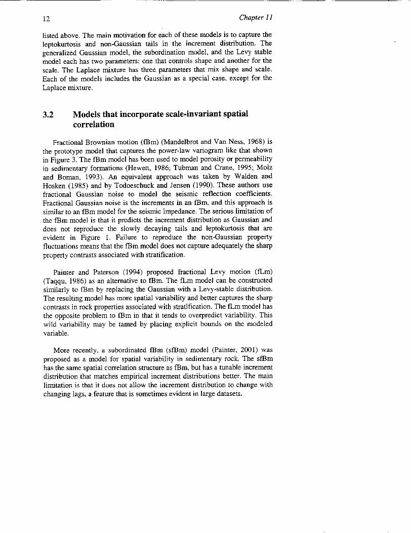
listed above. The main motivation for each of these models is to capture the leptokurtosis and non-Gaussian tails in the increment distribution. The generalized Gaussian model, the subordination model, and the Levy stable model each has two parameters: one that controls shape and another for the scale. The Laplace mixture has three parameters that mix shape and scale. Each of the models includes the Gaussian as a special case, except for the Laplace mixture.

3.2 Models that incorporate scale-invariant spatial correlation

Fractional Brownian motion (fBm) (Mandelbrot and Van Ness, 1968) is the prototype model that captures the power-law variogram like that shown in Figure 3. The fim model has been used to model porosity or permeability in sedimentary formations (Hewett, 1986; Tubman and Crane, 1995; Molz and Boman, 1993). An equivalent approach was taken by Walden and Hosken (1985) and by Todoeschuck and Jensen (1990). These authors use fractional Gaussian noise to model the seismic reflection coefficients. Fractional Gaussian noise is the increments in an fBm, and this approach is similar to an fBm model for the seismic impedance. The serious limitation of the fBm model is that it predicts the increment distribution as Gaussian and does not reproduce the slowly decaying tails and leptokurtosis that are evident in Figure 1. Failure to reproduce the non-Gaussian property fluctuations means that the fmm model does not capture adequately the sharp property contrasts associated with stratification.

Painter and Paterson (1994) proposed fractional Levy motion (fLm) (Taqqu, 1986) as an alternative to flim. The fLm model can be constructed similarly to fBm by replacing the Gaussian with a Levy-stable distribution. The resulting model has more spatial variability and better captures the sharp contrasts in rock properties associated with stratification. The fLm model has the opposite problem to fBm in that it tends to overpredict variability. This wild variability may be tamed by placing explicit bounds on the modeled variable.

More recently, a subordinated fBm (sfBm) model (Painter, 2001) was proposed as a model for spatial variability in sedimentary rock. The sfBm has the same spatial correlation structure as imm, but has a tunable increment distribution that matches empirical increment distributions better. The main limitation is that it does not allow the increment distribution to change with changing lags, a feature that is sometimes evident in large datasets.

Chapter I1112

11.

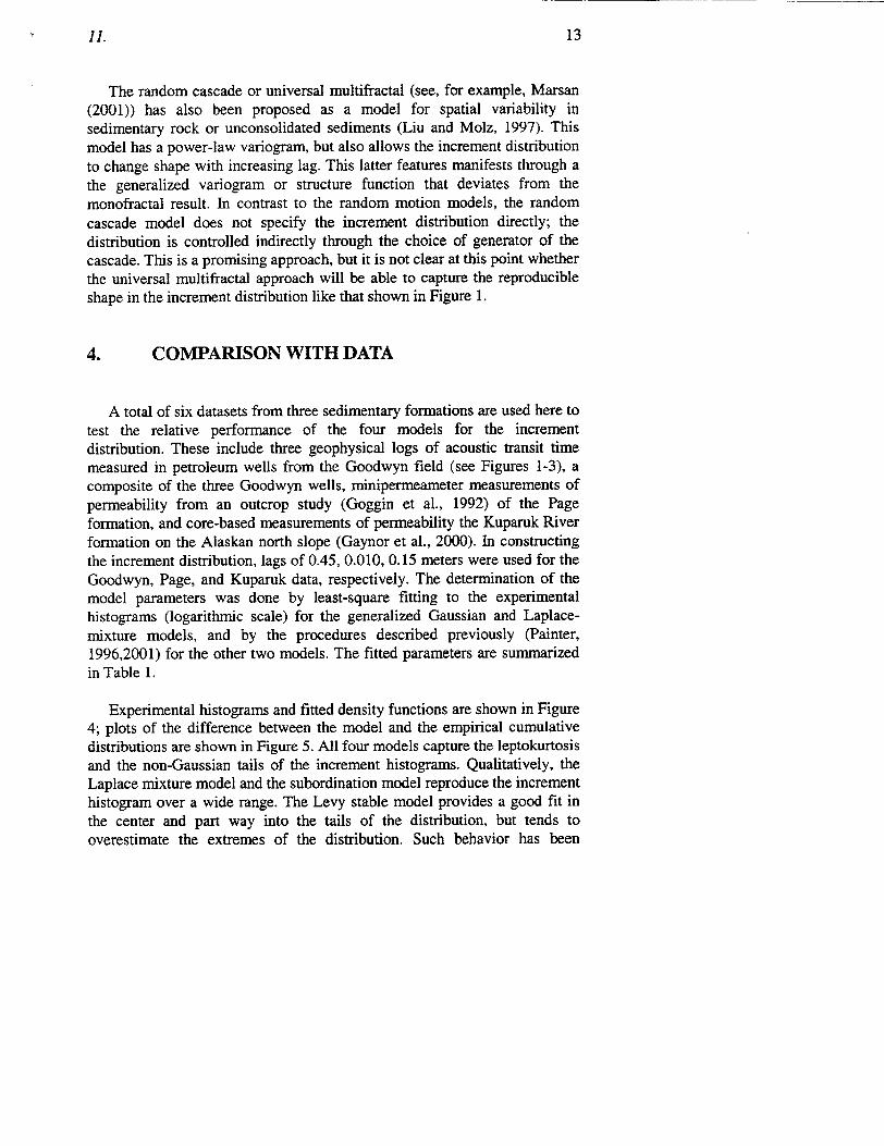
The random cascade or universal multifractal (see, for example, Marsan (2001)) has also been proposed as a model for spatial variability in sedimentary rock or unconsolidated sediments (Liu and Molz, 1997). This model has a power-law variogram, but also allows the increment distribution to change shape with increasing lag. This latter features manifests through a the generalized variogram or structure function that deviates from the monofractal result. In contrast to the random motion models, the random cascade model does not specify the increment distribution directly; the distribution is controlled indirectly through the choice of generator of the cascade. This is a promising approach, but it is not clear at this point whether the universal multifractal approach will be able to capture the reproducible shape in the increment distribution like that shown in Figure 1.

4. COMPARISON WITH DATA

A total of six datasets from three sedimentary formations are used here to test the relative performance of the four models for the increment distribution. These include three geophysical logs of acoustic transit time measured in petroleum wells from the Goodwyn field (see Figures 1-3), a composite of the three Goodwyn wells, minipermeameter measurements of permeability from an outcrop study (Goggin et al., 1992) of the Page formation, and core-based measurements of permeability the Kuparuk River formation on the Alaskan north slope (Gaynor et al., 2000). In constructing the increment distribution, lags of 0.45, 0.010, 0.15 meters were used for the Goodwyn, Page, and Kuparuk data, respectively. The determination of the model parameters was done by least-square fitting to the experimental histograms (logarithmic scale) for the generalized Gaussian and Laplacemixture models, and by the procedures described previously (Painter, 1996,2001) for the other two models. The fitted parameters are summarized in Table 1.

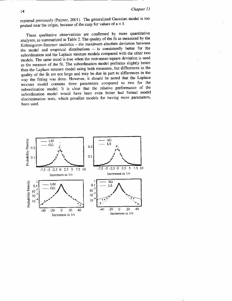
Experimental histograms and fitted density functions are shown in Figure 4; plots of the difference between the model and the empirical cumulative distributions are shown in Figure 5. All four models capture the leptokurtosis and the non-Gaussian tails of the increment histograms. Qualitatively, the Laplace mixture model and the subordination model reproduce the increment histogram over a wide range. The Levy stable model provides a good fit in the center and part way into the tails of the distribution, but tends to overestimate the extremes of the distribution. Such behavior has been

13

('Jinntpr 11]14 -1

reported previously (Painter, 2001). The generalized Gaussian model is too

peaked near the origin, because of the cusp for values of a < 1.

These qualitative observations are confirmed by more quantitative

analyses, as summarized in Table 2. The quality of the fit as measured by the

Kolmogorov-Smimov statistics - the maximum absolute deviation between

the model and empirical distributions - is consistently better for the

subordination and the Laplace mixture models compared with the other two

models. The same trend is true when the root-mean-square deviation is used

as the measure of the fit. The subordination model performs slightly better

than the Laplace mixture model using both measures, but differences in the

quality of the fit are not large and may be due in part to differences in the

way the fitting was done. However, it should be noted that the Laplace

mixture model contains three parameters compared to two for the

subordination model. It is clear that the relative performance of the

subordination model would have been even better had formal model

discrimination tests, which penalize models for having more parameters,

been used.

.LM - SG -------.. GG LS €

0.2 GG 0.2 ,

-C~0.1 0.1*

-7.5 -5 -2.5 0 2.5 5 7.5 10 -7.5 -5 -2.5 0 2.5 5 7.5 10

Increment in I/v Increment in 1/v

I1 I - SG "0.1 LS S0.1 G

1 2 GG---- 10-2 10 10

-3 -3 .-10 10.7

-44-4

.10 *10 *-

-40 -20 0 20 40 Increment in I/v

-20 0 20 Increment in INv

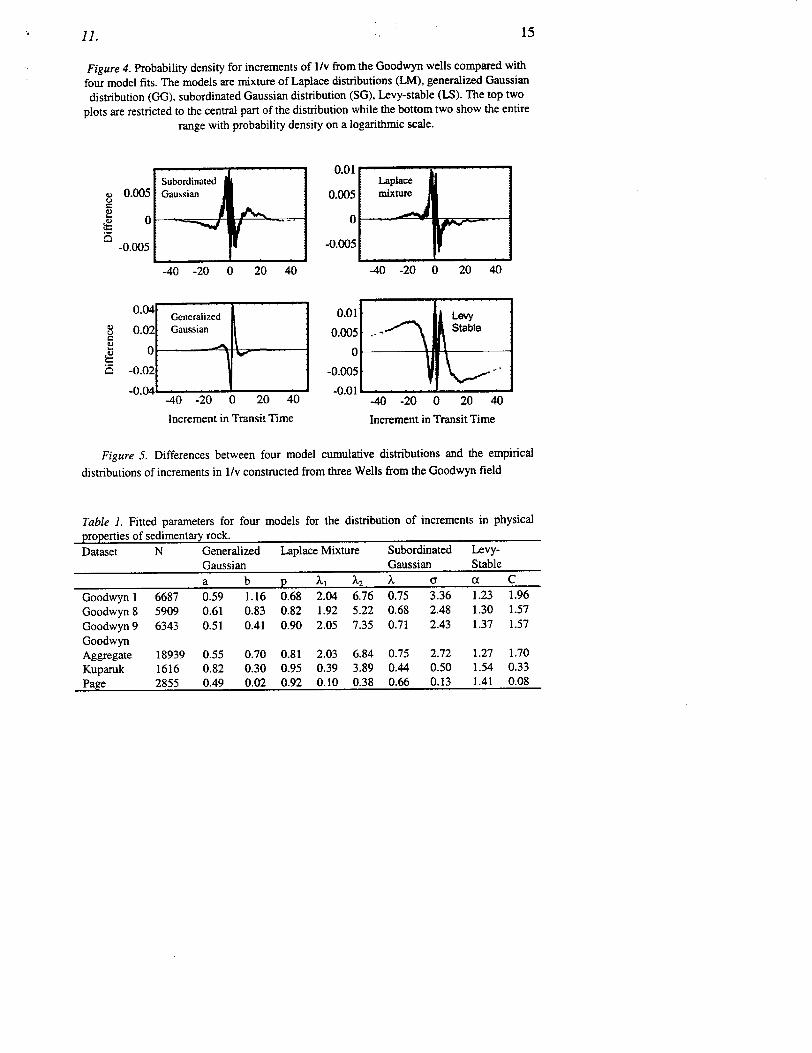
Figure 4. Probability density for increments of I/v from the Goodwyn wells compared with

four model fits. The models are mixture of Laplace distributions (LM), generalized Gaussian

distribution (GG). subordinated Gaussian distribution (SG), Levy-stable (LS). The top two

plots are restricted to the central part of the distribution while the bottom two show the entire range with probability density on a logarithmic scale.

-40 -20 0 20 40

Generalized Gaussian

--- I

-40 -20 0 20 40

Increment in Transit Time

0.0

0.00

-0.00

)1 Laplace

5 mixture

-40 -20 0 20 40

-40 -20 0 20 40

Increment in Transit Time

Figure 5. Differences between four model cumulative distributions and the empirical

distributions of increments in 1/v constructed from three Wells from the Goodwyn field

Table 1. Fitted parameters for four models for the distribution of increments in physical properties of sedimentary rock.

Dataset N Generalized Laplace Mixture Subordinated LevyGaussian Gaussian Stable

a b p X1 X2 , a a C

Goodwyn 1 6687 0.59 1.16 0.68 2.04 6.76 0.75 3.36 1.23 1.96

Goodwyn 8 5909 0.61 0.83 0.82 1.92 5.22 0.68 2.48 1.30 1.57

Goodwyn 9 6343 0.51 0.41 0.90 2.05 7.35 0.71 2.43 1.37 1.57 Goodwyn Aggregate 18939 0.55 0.70 0.81 2.03 6.84 0.75 2.72 1.27 1.70

Kuparuk 1616 0.82 0.30 0.95 0.39 3.89 0.44 0.50 1.54 0.33 PaLye 2855 0.49 0.02 0.92 0.10 0.38 0.66 0.13 1.41 0.08

Subordinated Gaussian A,u 0.005

S0

-0.005

0.04

S0.02 2 0 S -0.02

-- I a

1511.

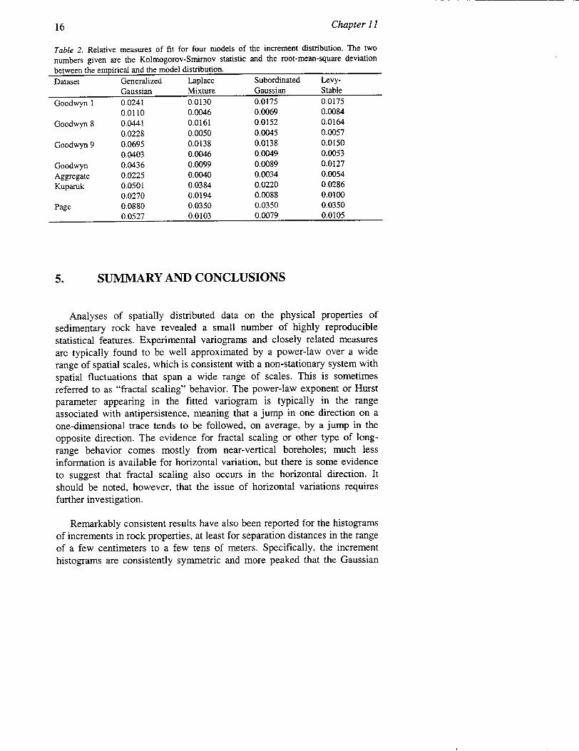
Table 2. Relative measures of fit for four models of the increment distribution. The two

numbers given are the Kolmogorov-Smirnov statistic and the root-mean-square deviation

between the empirical and the model distribution.

Dataset Generalized Laplace Subordinated LevyGaussian Mixture Gaussian Stable

Goodwyn 1 0.0241 0.0130 0.0175 0.0175

0.0110 0.0046 0.0069 0.0084

Goodwyn 8 0.0441 0.0161 0.0152 0.0164

0.0228 0.0050 0.0045 0.0057

Goodwyn 9 0.0695 0.0138 0.0138 0.0150 0.0403 0.0046 0.0049 0.0053

Goodwyn 0.0436 0.0099 0.0089 0.0127

Aggregate 0.0225 0.0040 0.0034 0.0054

Kuparuk 0.0501 0.0384 0.0220 0.0286

0.0270 0.0194 0.0088 0.0100 Page 0.0880 0.0350 0.0350 0.0350

0.0527 0.0103 0.0079 0.0105

5. SUMMARY AND CONCLUSIONS

Analyses of spatially distributed data on the physical properties of sedimentary rock have revealed a small number of highly reproducible statistical features. Experimental variograms and closely related measures are typically found to be well approximated by a power-law over a wide range of spatial scales, which is consistent with a non-stationary system with spatial fluctuations that span a wide range of scales. This is sometimes referred to as "fractal scaling" behavior. The power-law exponent or Hurst parameter appearing in the fitted variogram is typically in the range associated with antipersistence, meaning that a jump in one direction on a one-dimensional trace tends to be followed, on average, by a jump in the opposite direction. The evidence for fractal scaling or other type of longrange behavior comes mostly from near-vertical boreholes; much less information is available for horizontal variation, but there is some evidence to suggest that fractal scaling also occurs in the horizontal direction. It should be noted, however, that the issue of horizontal variations requires further investigation.

Remarkably consistent results have also been reported for the histograms of increments in rock properties, at least for separation distances in the range of a few centimeters to a few tens of meters. Specifically, the increment histograms are consistently symmetric and more peaked that the Gaussian

Chapter I1I16

11. 17

density, and have tails that decay more slowly than the Gaussian. There is

some evidence to suggest that the increment distribution trends toward

Gaussian with increasing separation distance, although the exact nature of

this trend and the crossover point to Gaussian behavior is somewhat

uncertain. The consistent non-Gaussian shape has been observed for both

horizontal and vertical separation distances. The width in the observed

distribution tends to be smaller in the horizontal direction, consistent with

reduced variability in the horizontal compared with the vertical.

Several models for the increment distribution have been put forward in

the groundwater, petroleum engineering, and exploration geophysics

literatures. The performance of four of these models is compared using data

from several sources. A model based on a mixture of two Laplace

distributions and a model based on subordination of a Gaussian process both

outperformed models based on a Levy-stable distribution and a generalized

Gaussian distribution. The generalized Gaussian model is more peaked than

the increment histograms and the Levy stable model predicts too much

probability density in the tails of the distribution. The Laplace mixture

model and the subordination model fit the histograms well over a wide range

of increment values, but the fit of the subordination model is slightly better.

The subordination model also has fewer parameters and is thus preferred

from the perspective of parsimony. Moreover, the subordinated fBm model

also allows models the observed spatial correlation.

ACKNOWLEDGMENTS

This work was performed in part by the Center for Nuclear Waste

Regulatory Analyses under contract NRC-02-97-009. This report is an

independent product and does not necessarily reflect the regulatory position of the NRC.

REFERENCES

Agard, J., 1961, L'analyses statistique et probabiliste des sismogrammes, Revue de L'Institut

Francais du Pitrole 16:1-85.

Feller, W., 1971, An introduction to probability theory and its applications Vol. 2, Wiley and

Sons, Inc., New York?.

18 Chapter 11

Gelhar, L. M., 1993, Stochastic subsurface hydrology, Prentice Hall, Englewood Cliffs, New

Jersey.

Goggin, D. J., Chandler, M. A., Kocurek, G., and Lake, L. W., 1992, Permeability transects of

eolian sands and their use in generating random permeability fields, SPE Formation

Evaluation 92(3):7-16.

Hewett, T. A., 1986, Fractal distributions of reservoir heterogeneity and their influence on

fluid transport, in: Proceedings of the 61' Annual Technical Conference of the Society of

Petroleum Engineers, Rep. 15386, Richardson Texas.

Journel, A. G., and Huijbregts, Ch. J., 1978, Mining Geostatistics, Academic Press, New

York.

Krige, D. G., 1970. The role of mathematical statistics in improving ore valuation techniques

in South African gold mines, in: Topics in Mathematical Geology, Consultants Bureau,

New York and London.

Lavy, P., 1937, The4orie de I'addition des variables algatoires, Gauthier-Villars, Paris.

Liu, H. H., and Molz, F. J., 1997a, Comment on "Evidence for non-Gaussian scaling behavior

in heterogeneous sedimentary formations" by Scott Painter, Water Resour. Res.

33(4):907-908.

Liu, H. H., and Molz, F. J., 1997b, Multifractal analyses of hydraulic conductivity

distributions, Water Resour. Res. 33(11):2483-2488.

Mandelbrot, B. B., 1969, Robustness of the rescaled range R/S in the measurement of

noncyclic long run statistical dependence, Water Resources Research 5:967-988.

Mandelbrot, B. B. and Van Ness, J. W., 1968, Fractional Brownian motions, fractional noises

and applications, SIAM Rev. 10:422-437.

Molz, F. J., and Boman, G. K., 1993, A fractal-based stochastic interpolation scheme in

subsurface hydrology, Water Resour. Res. 29(11):3769-3774.

Molz, F. J., and Boman, G. K., 1995, Further evidence of fractal structure in hydraulic

conductivity distributions, Geophys. Res. Lett. 22:2545-2548.

Neuman, S. P., 1990. Universal scaling of hydraulic conductivities and dispersivities in

geological media, Water Resour. Res. 26(8):1749-1758.

Neuman, S. P., 1994. Generalized scaling of permeability: Validation and effect of support

scale, Geophys. Res. Lett. 21(5):349-352.

O'Doherty, R. F., and Anstey, N. A., 1971, Reflections on amplitudes, Geophys. Prosp. 19:440-458.

Painter, S., 1995, Random fractal models of heterogeneity: The Levy-stable approach, Math.

Geol. 27:813-830.

11. 19

Painter, S., 1996, Evidence for non-Gaussian scaling behavior in heterogeneous sedimentary formations, Water Resour. Res. 32(5): 1183-1195.

Painter, S., 2001, Flexible scaling model for use in random field simulation of hydraulic conductivity, Water Resour. Res. In press.

Painter, S, and Paterson, L., 1994, Fractional Levy motion as a model for spatial variability in

sedimentary rock, Geophys. Res. Lens. 21:2857-2860.

Painter, S., Beresford, G., and Paterson, L., 1995, On the distribution of seismic reflection coefficients and seismic amplitudes, Geophysics 60(4):1187-1194.

Pilkington, M., and Todoeschuck, J. P., 1990, Stochastic inversion for scaling geology, Geophys. J. Internat. 102:205-217.

Todoeschuck, J. P., and Jenson, 0. G., 1988, Scaling geology and seismic deconvolution. Geophysics 53:1410-1414.

Walden, A. T., and Hosken, J. W. J., 1985, An investigation of the spectral properties of

primary reflection coefficients, Geophys. Prosp. 33:400-435.

Walden, A. T., and Hosken, J. W. J., 1986, The nature of the non-gaussianity of primary

reflection coefficients and its significance for deconvolution, Geophys. Prosp. 34:10381066.

Zolotarev, V. M., 1986, One-dimensional stable distributions, Am. Math. Soc.