Lrz kurs: gpu and mic programming with r
73
GPU and MIC programming (using python, R and MATLAB) * Ferdinand Jamitzky ([email protected]) http://goo.gl/JkYJFY
-
Upload
ferdinand-jamitzky -
Category
Education
-
view
108 -
download
2
Transcript of Lrz kurs: gpu and mic programming with r

GPU and MIC programming (using python, R and MATLAB)
*
Ferdinand Jamitzky ([email protected])
http://goo.gl/JkYJFY

Moore’s Law
Number of transistors
doubles every 2 years

Why parallel programming?
End of the free lunch
in 2000 (heat death)
Moore's law means
not faster processors,
only more of them.
But!
2 x 3 GHz < 6 GHz
(cache consistency,
multi-threading, etc)

From Supercomputers to Notebook PCs

The future was (always) massively parallel
Connection Machine
CM-1 (1983)
12-D Hypercube
65536 1-bit cores
(AND, OR, NOT)
Rmax: 20 GFLOP/s
Today’s notebook PC

The future is massively parallel
JUGENE
Blue Gene/P (2007)
3-D Torus or Tree
65536 64-bit cores
(PowerPC 450)
Rmax: 222 TFLOP/s
now: 1 PFLOP/s
294912 cores

Problem: Moving Data/Latency
Getting data from:
CPU register 1ns
L2 cache 10ns
memory 80 ns
network(IB) 200 ns
GPU(PCIe) 50.000 ns
harddisk 500.000 ns
Light ray travels:
30 cm
3 m
24 m
60 m
15 km
150 km

Problem: Transport energy
Moving Data is expensive:
FLOP on CPU 170 pJ
FLOP on GPU 20 pJ
Read from RAM 16000 pJ
Wire 10 cm 3100 pJ
Wire per mm 0.15 pJ/bit/cm
source: http://www.davidglasco.com/Papers/ieee-micro.pdf and W. Dally (nVidia)

Data hungry...
Getting data from:
CPU register 1ns
L2 cache 10ns
memory 80 ns
network(IB) 200 ns
GPU(PCIe) 50.000 ns
harddisk 500.000 ns
Getting some food from:
fridge 10s
microwave 100s ~ 2min
pizza service 800s ~ 15min
city mall 2000s ~ 0.5h
mum sends cake 500.000 s~1 week
grown in own garden 5Ms ~ 2months

Supercomputer: SMP
SMP Machine:
shared memory
typically 10s of cores
threaded programs
bus interconnect
in R:
library(multicore)
and inlined code
Example: gvs1
128 GB RAM
16 cores
Example: uv2/3
3.359 GB RAM
2.080 cores

Supercomputer: MPI
Cluster of machines:
distributed memory
typically 100s of cores
message passing interface
infiniband interconnect
in R:
library(Rmpi)
and inlined code
Example: linux MPP cluster
2,752 GB RAM
2,752 cores
Example: superMUC
340,000 GB RAM
155,656 Intel cores

Supercomputer: GPGPU
Graphics Card:
shared memory
typically 1000s of cores
CUDA or openCL
on chip interconnect
in R:
library(gputools)
and dyn.load code
Example: Tesla K20X
6 GB RAM
2688 Threads
Example: Titan ORNL
262,000 GB RAM
18,688 GPU Cards
50,233,344 Threads

Supercomputer: MIC
Many Core Accelerator:
shared memory
60 cores
offload or native
on chip interconnect
in R:
MKL auto-offload
and dyn.load code
Example: SuperMIC
8 GB RAM
240 Threads
Example: Tianhe-2
1,024,000 GB RAM
3,120,000 cores

Levels of Parallelism
●Node Level (e.g. SuperMUC has approx. 10000 nodes)
each node has 2 sockets
●Socket Level
each socket contains 8 cores
●Core Level
each core has 16 vector registers
●Vector Level (e.g. lxgp1 GPGPU has 480 vector registers)
●Pipeline Level (how many simultaneous pipelines)
hyperthreading
●Instruction Level (instructions per cycle)
out of order execution, branch prediction, FMA

Amdahl's law
Computing time for N processors
T(N) = T(1)/N + Tserial + Tcomm * N
Acceleration factor (Speedup)
T(1)/T(N) = N / (1 + Tserial/T(1)*N + Tcomm/T(1)*N^2)
small N Speedup: T(1)/T(N) ~ N
large N Speedup: T(1)/T(N) ~ T(1)/Tcomm * 1/N
saturation point!

Amdahl's law
> plot(N,type="l")
> lines(N/(1+0.01*N+0.001*N**2),col="green")
> lines(N/(1+0.01*N),col="red")
> Tserial=0.01
> Tcomm=0.001

Gustafson's law
large N Speedup: T(1proc)/T(Nproc) ~ T(1proc)/Tcomm * 1/N
Grow your problem then it scales better.
Weak Scaling
vs.
Strong Scaling
e.g. molecular
simulations:
100 atoms/core
are needed

How are High-Performance Codes
constructed?
●“Traditional” Construction of High-Performance Codes:
oC/C++/Fortran
oLibraries
●“Alternative” Construction of High-Performance Codes:
oScripting for ‘brains’ (Computer Games: Logic, AI)
oGPUs for ‘inner loops’ (Computer Games: Visualisation)
●Play to the strengths of each programming environment.

Hierarchical architecture of
hardware vs software
●accelerators (gpus, xeon phi)
●in-core vectorisation (avx)
●multicore nodes (qpi, pci bus)
●strongly coupled nodes (infiniband, 10GE)
●weakly coupled clusters (cloud)
●Cuda, intrinsics
●vectorisation pragmas
●openMP
●MPI
●workflow middleware

Why Scripting?
Do you:
●want to reuse CUDA code easily (e.g. as a library) ?
●want to dynamically determine whether CUDA is available?
●want to use multi-threading (painlessly)?
●want to use MPI (painlessly)?
●want to use loose coupling (grid computing)?
●want dynamic exception handling and fallbacks?
●want dynamic compilation of CUDA code?
If you answered "yes" to one of these questions, you
should consider a scripting language

Parallel Tools in python, R and MATLAB
SMP
multicore
parallelism
doMC, doSMP,
pnmath, BLAS
no max cores
multiprocessing
futures
MMP massive
parallel
processing
doSNOW,
doMPI, doRedis
parallel python,
mpi4py
GPGPU
CUDA
openCL
rgpu, gputools
pyCUDA,
pyOpenCL
parfor, spmd
max 8 cores
jobs, pmode gpuArray
R
python
MATLAB
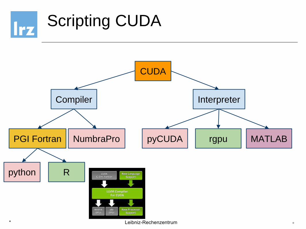
Scripting CUDA
Compiler
CUDA
Interpreter
PGI Fortran NumbraPro pyCUDA rgpu MATLAB
python R

MATLAB GPU Commands

MATLAB GPU @ LRZ
# load matlab module and start command line version
module load cuda
module load matlab/R2011A
matlab -nodesktop

MATLAB gpuArray
●Copy data to GPGPU and return a handle on the object
●All operations on the handle are performed on the GPGPU
x=rand(100);
gx=gpuArray(x);
●how to compute the GFlop/s
tic;
M=gpuArray(rand(np*1000));
gather(sum(sum(M*M)));
2*np^3/toc
pyCUDA
Gives you the following advantages:
1.Combining Two Strong Tools
2.Scripting CUDA
3.Run-Time Code Generation
http://mathema.tician.de/software/pycuda
special thanks to a.klöckner

pyCUDA @ LRZ
log in to lxgp1
$ module load python
$ module load cuda
$ module load boost
$ python
Python 2.6.1 (r261:67515, Apr 17 2009, 17:25:25)
[GCC 4.1.2 20070115 (SUSE Linux)] on linux2
Type "help", "copyright", "credits" or "license" for more
information.
>>>

Simple Example
from numpy import *
import pycuda.autoinit
import pycuda.gpuarray as gpu
a_gpu =
gpu.to_gpu(random.randn(4,4).astype(float32))
a_doubled = (2∗a_gpu).get()
print a_doubled
print a_gpu

gpuarray class
pycuda.gpuarray:
Meant to look and feel just like numpy.
●gpuarray.to gpu(numpy array)
●numpy array = gpuarray.get()
●+, -, ∗, /, fill, sin, exp, rand, basic indexing, norm, inner product
●Mixed types (int32 + float32 = float64)
●print gpuarray for debugging.
●Allows access to raw bits
●Use as kernel arguments, textures, etc.

gpuarray: Elementwise expressions
Avoiding extra store-fetch cycles for elementwise math:
from pycuda.curandom import rand as curand
a_gpu = curand((50,))
b_gpu = curand((50,))
from pycuda.elementwise import ElementwiseKernel
lin_comb = ElementwiseKernel(
” float a, float ∗x, float b, float ∗y, float ∗z”,”z[ i ] = a∗x[i ] + b∗y[i]”)
c_gpu = gpuarray.empty_like (a_gpu)
lin_comb(5, a_gpu, 6, b_gpu, c_gpu)
assert la.norm((c_gpu − (5∗a_gpu+6∗b_gpu)).get()) < 1e−5

gpuarray: Reduction made easy
Example: A scalar product calculation
from pycuda.reduction import ReductionKernel
dot = ReductionKernel(dtype_out=numpy.float32, neutral=”0”,
reduce_expr=”a+b”, map_expr=”x[i]∗y[i]”,arguments=”const float ∗x, const float ∗y”)
from pycuda.curandom import rand as curand
x = curand((1000∗1000), dtype=numpy.float32)y = curand((1000∗1000), dtype=numpy.float32)
x_dot_y = dot(x,y).get()
x_dot_y_cpu = numpy.dot(x.get(), y.get ())

CUDA Kernels in pyCUDA
import pycuda.autoinit
import pycuda.driver as drv
import numpy
from pycuda.compiler import SourceModule
mod = SourceModule("""
__global__ void multiply_them(float *dest, float *a, float *b)
{ const int i = threadIdx.x;
dest[i] = a[i] * b[i];
}""")
multiply_them = mod.get_function("multiply_them")
a = numpy.random.randn(400).astype(numpy.float32)
b = numpy.random.randn(400).astype(numpy.float32)
dest = numpy.zeros_like(a)
multiply_them(
drv.Out(dest), drv.In(a), drv.In(b),
block=(400,1,1)
print dest-a*b

Completeness
PyCUDA exposes all of CUDA.
For example:
●Arrays and Textures
●Pagelocked host memory
●Memory transfers (asynchronous, structured)
●Streams and Events
●Device queries
●GL Interop
And furthermore:
●Allow interactive use
●Integrate tightly with numpy

pyCUDA showcase
http://wiki.tiker.net/PyCuda/ShowCase
●Agent-based Models
●Computational Visual Neuroscience
●Discontinuous Galerkin Finite Element PDE Solvers
●Estimating the Entropy of Natural Scenes
●Facial Image Database Search
●Filtered Backprojection for Radar Imaging
●LINGO Chemical Similarities
●Recurrence Diagrams
●Sailfish: Lattice Boltzmann Fluid Dynamics
●Selective Embedded Just In Time Specialization
●Simulation of spiking neural networks

NumbraPro
Generate CUDA Kernels using a Just-in-time compiler
from numbapro import cuda
@cuda.jit('void(float32[:], float32[:], float32[:])')
def sum(a, b, result):
i = cuda.grid(1) # equals to threadIdx.x + blockIdx.x *
blockDim.x
result[i] = a[i] + b[i]
# Invoke like: sum[grid_dim, block_dim](big_input_1, big_input_2,
result_array)

R in a nutshell
module load cuda/2.3
module load R/serial/2.13
> x=1:10
> y=x**2
> str(y)
> print(x)
> times2 = function(x) 2*x
graphics!> plot(x,y)
= and <- are interchangable
rgpu
a set of functions for loading data toa gpu and manipulating the
data there:
●exportgpu(x)
●evalgpu(x+y)
●lsgpu()
●rmgpu("x")
●sumgpu(x), meangpu(x), gemmgpu(a,b)
●cos, sin,.., +, -, *, /, **, %*%

Example
load the correct R module
$ module load R/serial/2.13
start R
$ R
R version 2.13.1 (2011-07-08)
Copyright (C) 2011 The R Foundation for Statistical Computing
ISBN 3-900051-07-0
load rgpu library
> library(rgpu)
> help(package="rgpu")
> rgpudetails()

Data on the GPGPU
one million random uniform numbers
> x=runif(10000000)
send data to gpu
> exportgpu(x)
do some calculations
> evalgpu(sumgpu(sin(x)+cos(x)+tan(x)+exp(x)))
do some timing comparisons (GPU vs CPU):
> system.time(evalgpu(sumgpu(sin(x)+cos(x)+tan(x)+exp(x))))
> system.time(sum(sin(x)+cos(x)+tan(x)+exp(x)))
real world examples: gputools
gputools is a package of precompiled CUDA functions for
statistics, linear algebra and machine learning
●chooseGpu
●getGpuId()
●gpuCor, gpuAucEstimate
●gpuDist, gpuDistClust, gpuHclust, gpuFastICA
●gpuGlm, gpuLm
●gpuGranger, gpuMi
●gpuMatMult, gpuQr, gpuSvd, gpuSolve
●gpuLsfit
●gpuSvmPredict, gpuSvmTrain
●gpuTtest

Example: Matrix Inversion
np <- 2000
x <- matrix(runif(np**2), np,np)
system.time(gpuSolve(x))
system.time(solve(x))

Example: Hierarchical Clustering
numVectors <- 5
dimension <- 10
Vectors <- matrix(runif(numVectors*dimension), numVectors,
dimension)
distMat <- gpuDist(Vectors, "euclidean")
myClust <- gpuHclust(distMat, "single")
plot(myClust)
for other examples try:
example(hclust)

Fortran 90 Example
program myprog
! simulate harmonic oscillator
integer, parameter :: np=1000, nstep=1000
real :: x(np), v(np), dx(np), dv(np), dt=0.01
integer :: i,j
forall(i=1:np) x(i)=i
forall(i=1:np) v(i)=i
do j=1,nstep
dx=v*dt; dv=-x*dt
x=x+dx; v=v+dv
end do
print*, " total energy: ",sum(x**2+v**2)
end program

PGI Compiler
log in to lxgp1
$ module load fortran/pgi/11.8
$ pgf90 -o myprog.exe myprog.f90
$ time ./myprog.exe
exercise for you:
●compute MFlop/s (Floating Point Operations: 4 * np * nstep)
●optimize (hint: -Minfo, -fast, -O3)

Fortran 90 Example
program myprog
! simulate harmonic oscillator
integer, parameter :: np=1000, nstep=1000
real :: x(np), v(np), dx(np), dv(np), dt=0.01
integer :: i,j
forall(i=1:np) x(i)=i
forall(i=1:np) v(i)=i
do j=1,nstep
!$acc region
dx=v*dt; dv=-x*dt
x=x+dx; v=v+dv
!$acc end region
end do
print*, " total energy: ",sum(x**2+v**2)
end program

PGI Compiler accelerator
module load fortran/pgi
pgf90 -ta=nvidia -o myprog.exe myprog.f90
time ./myprog.exe
exercise for you:
●compute MFlop/s (Floating Point Operations: 4 * np * nstep)
●optimize (hint: change acc region)
Use R as scripting language
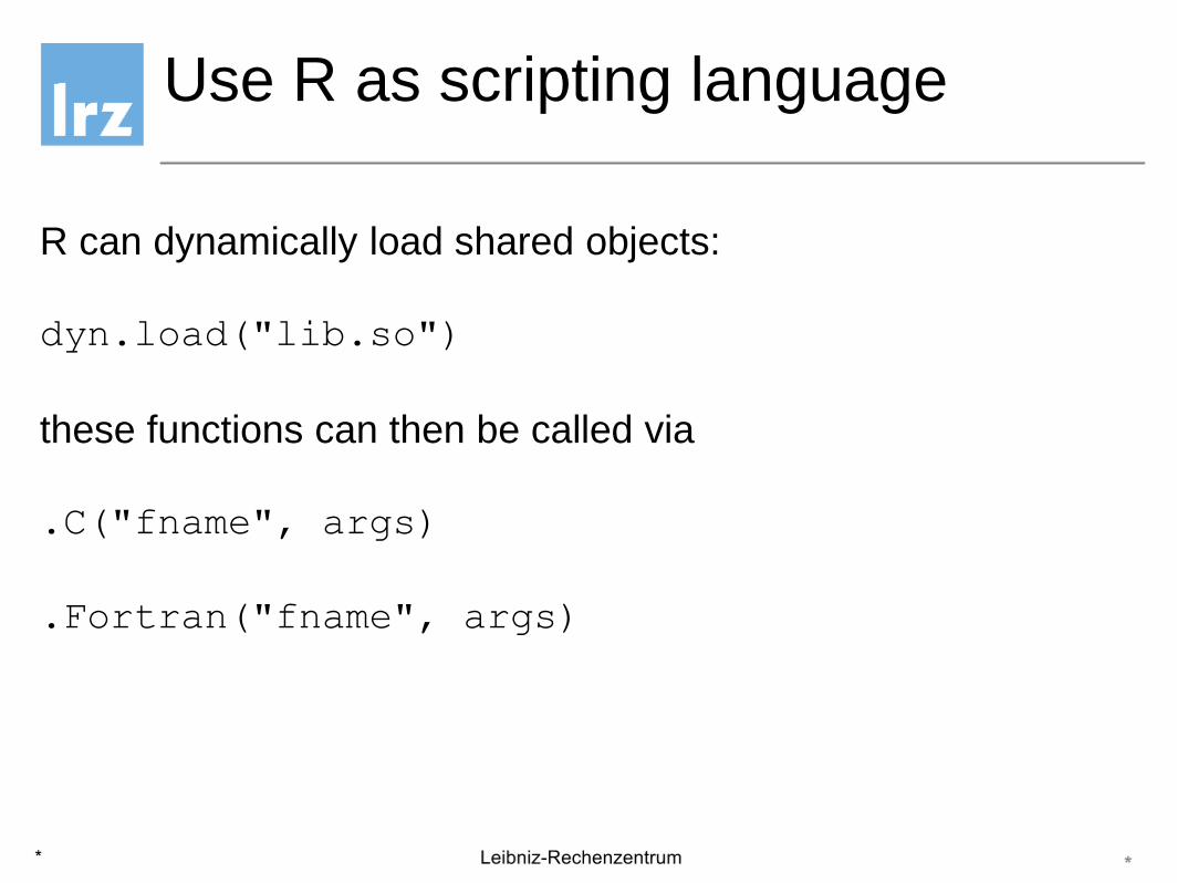
R can dynamically load shared objects:
dyn.load("lib.so")
these functions can then be called via
.C("fname", args)
.Fortran("fname", args)

R subroutine
subroutine mysub_cuda(x,v,nstep)
! simulate harmonic oscillator
integer, parameter :: np=1000000
real*8 :: x(np), v(np), dx(np), dv(np), dt=0.001
integer :: i,j, nstep
forall(i=1:np) x(i)=real(i)/np
forall(i=1:np) v(i)=real(i)/np
do j=1,nstep
dx=v*dt; dv=-x*dt
x=x+dx; v=v+dv
end do
return
end subroutine

Compile two versions
don't forget to load the modules!module unload ccomp fortran
module load ccomp/pgi/11.8
module load fortran/pgi/11.8
module load R/serial/2.13
pgf90 -shared -fPIC -o mysub_host.so
mysub_host.f90
pgf90 -ta=nvidia -shared -fPIC -o
mysub_cuda.so mysub_cuda.f90

Load and run
Load dynamic libraries> dyn.load("mysub_host.so"), dyn.load("mysub_cuda.so"); np=1000000
Benchmark> system.time(str(.Fortran("mysub_host",x=numeric(np),v=numeric(np),nstep=as.integer(1000))))
total energy: 666667.6633012500
total energy: 667334.6641391169
List of 3
$ x : num [1:1000000] -3.01e-07 -6.03e-07 -9.04e-07 -1.21e-06 -1.51e-06 ...
$ v : num [1:1000000] 1.38e-06 2.76e-06 4.15e-06 5.53e-06 6.91e-06 ...
$ nstep: int 1000
user system elapsed
26.901 0.000 26.900
> system.time(str(.Fortran("mysub_cuda",x=numeric(np),v=numeric(np),nstep=as.integer(1000))))
total energy: 666667.6633012500
total energy: 667334.6641391169
List of 3
$ x : num [1:1000000] -3.01e-07 -6.03e-07 -9.04e-07 -1.21e-06 -1.51e-06 ...
$ v : num [1:1000000] 1.38e-06 2.76e-06 4.15e-06 5.53e-06 6.91e-06 ...
$ nstep: int 1000
user system elapsed
0.829 0.000 0.830
Acceleration Factor:> 26.9/0.83
[1] 32.40964
Matrix Multipl. in FORTRAN
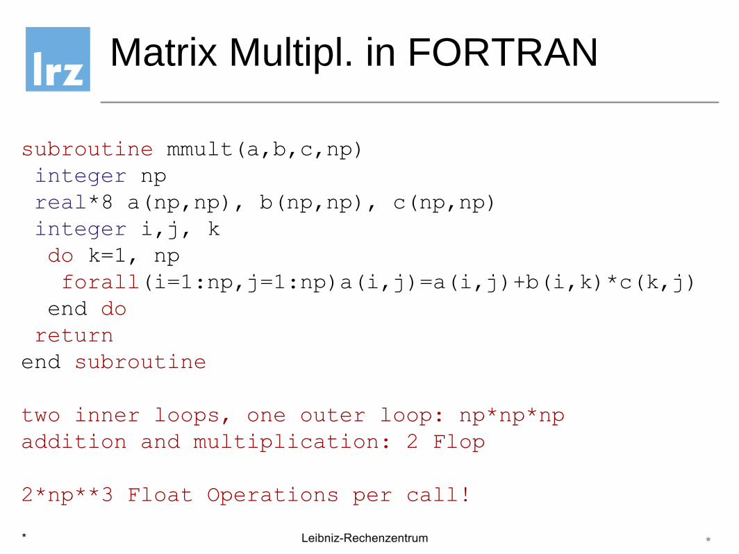
subroutine mmult(a,b,c,np)
integer np
real*8 a(np,np), b(np,np), c(np,np)
integer i,j, k
do k=1, np
forall(i=1:np,j=1:np)a(i,j)=a(i,j)+b(i,k)*c(k,j)
end do
return
end subroutine
two inner loops, one outer loop: np*np*np
addition and multiplication: 2 Flop
2*np**3 Float Operations per call!

Call FORTRAN from R
# compile f90 to shared object library
system("pgf90 -shared -fPIC -o mmult.so
mmult.f90");
# dynamically load library
dyn.load("mmult.so")
# define multiplication function
mmult.f <- function(a,b,c)
.Fortran("mmult",a=a,b=b,c=c,
np=as.integer(dim(a)[1]))

Call FORTRAN binary
np=100
system.time(
mmult.f(
a = matrix(numeric(np*np),np,np),
b = matrix(numeric(np*np)+1.,np,np),
c = matrix(numeric(np*np)+1.,np,np)
)
)
Exercise: make a plot system-time vs matrix-dimension
PGI accelerator directives
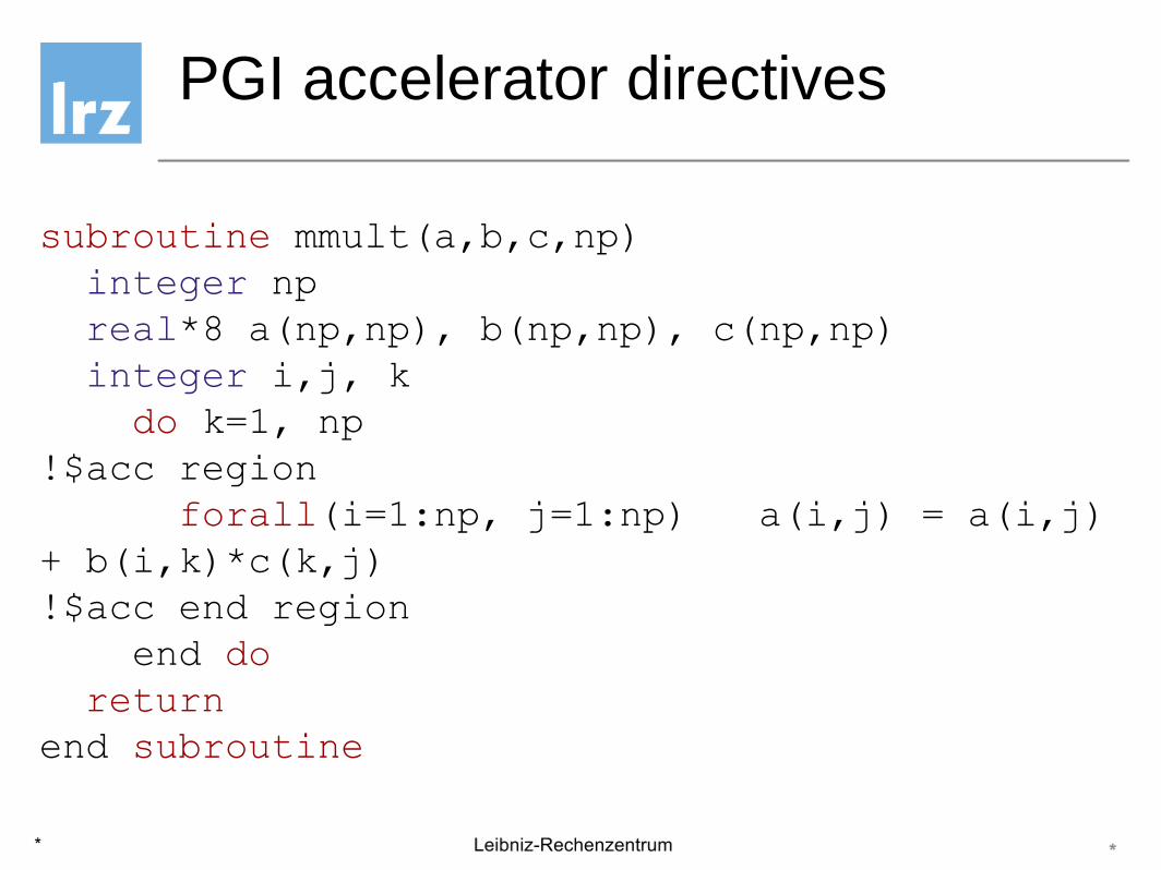
subroutine mmult(a,b,c,np)
integer np
real*8 a(np,np), b(np,np), c(np,np)
integer i,j, k
do k=1, np
!$acc region
forall(i=1:np, j=1:np) a(i,j) = a(i,j)
+ b(i,k)*c(k,j)
!$acc end region
end do
return
end subroutine

Call FORTRAN from R
# compile f90 to shared object library
system("pgf90 -ta=nvidia -shared -fPIC -o
mmult.so mmult.f90");
# dynamically load library
dyn.load("mmult.so")
# define multiplication function
mmult.f <- function(a,b,c)
.Fortran("mmult",a=a,b=b,c=c,
np=as.integer(dim(a)[1]))

Compute MFlop/s
print(paste(2.*np**3/1000000./system.time(
str(mmult.f(...))
)[[3]]," MFlop/s"))
Exercise: Compare MFlop/s vs dimension for serial and
accelerated code

Intel accelerator directives
subroutine mmult(a,b,c,np)
integer np
real*8 a(np,np), b(np,np), c(np,np)
integer i,j, k
!dir$ offload begin target(mic) inout(a,b,c)
!$omp parallel shared(a,b,c)
!$omp do
do j=1,np
do k=1,np
forall(i=1:np) a(i,j)=a(i,j)+b(i,k)*c(k,j)
end do
end do
!$omp end do
!$omp end parallel
!dir$ end offload
return
end subroutine

Compiler command Intel Fortran
$ ifort -vec-report=3 -openmp-report -openmp -shared -fPIC mmult_mic.f90 -o mmult_mic.so
mmult_omp.f90(7): (col. 7) remark: OpenMP DEFINED LOOP WAS PARALLELIZED
mmult_omp.f90(6): (col. 7) remark: OpenMP DEFINED REGION WAS PARALLELIZED
mmult_omp.f90(10): (col. 20) remark: LOOP WAS VECTORIZED
mmult_omp.f90(9): (col. 3) remark: loop was not vectorized: not inner loop
mmult_omp.f90(8): (col. 1) remark: loop was not vectorized: not inner loop
mmult_omp.f90(7): (col. 7) remark: *MIC* OpenMP DEFINED LOOP WAS PARALLELIZED
mmult_omp.f90(6): (col. 7) remark: *MIC* OpenMP DEFINED REGION WAS PARALLELIZED
mmult_omp.f90(10): (col. 20) remark: *MIC* LOOP WAS VECTORIZED
mmult_omp.f90(10): (col. 20) remark: *MIC* PEEL LOOP WAS VECTORIZED
mmult_omp.f90(10): (col. 20) remark: *MIC* REMAINDER LOOP WAS VECTORIZED
mmult_omp.f90(9): (col. 3) remark: *MIC* loop was not vectorized: not inner loop
mmult_omp.f90(8): (col. 1) remark: *MIC* loop was not vectorized: not inner loop

mmult on MIC (offload)
$ R -f mmult_mic.R
> system.time(mmult.f(a,b,c))
[Offload] [MIC 0] [File] mmult_mic.f90
[Offload] [MIC 0] [Line] 5
[Offload] [MIC 0] [Tag] Tag 0
[Offload] [HOST] [Tag 0] [CPU Time] 173.768076(seconds)
[Offload] [MIC 0] [Tag 0] [CPU->MIC Data] 2400000280 (bytes)
[Offload] [MIC 0] [Tag 0] [MIC Time] 155.217991(seconds)
[Offload] [MIC 0] [Tag 0] [MIC->CPU Data] 2400000016 (bytes)
user system elapsed
157.034 2.844 176.542
> system.time(b%*%c)
[MKL] [MIC --] [AO Function] DGEMM
[MKL] [MIC --] [AO DGEMM Workdivision] 0.50 0.25 0.25
[MKL] [MIC 00] [AO DGEMM CPU Time] 5.699716 seconds
[MKL] [MIC 00] [AO DGEMM MIC Time] 1.142100 seconds
[MKL] [MIC 00] [AO DGEMM CPU->MIC Data] 1001600000 bytes
[MKL] [MIC 00] [AO DGEMM MIC->CPU Data] 806400000 bytes
[MKL] [MIC 01] [AO DGEMM CPU Time] 5.699716 seconds
[MKL] [MIC 01] [AO DGEMM MIC Time] 1.255698 seconds
[MKL] [MIC 01] [AO DGEMM CPU->MIC Data] 1001600000 bytes
[MKL] [MIC 01] [AO DGEMM MIC->CPU Data] 806400000 bytes
user system elapsed
42.414 6.492 6.326
mmult on host (16c) vs MIC
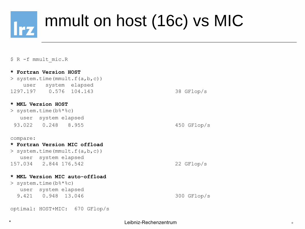
$ R -f mmult_mic.R
* Fortran Version HOST
> system.time(mmult.f(a,b,c))
user system elapsed
1297.197 0.576 104.143 38 GFlop/s
* MKL Version HOST
> system.time(b%*%c)
user system elapsed
93.022 0.248 8.955 450 GFlop/s
compare:
* Fortran Version MIC offload
> system.time(mmult.f(a,b,c))
user system elapsed
157.034 2.844 176.542 22 GFlop/s
* MKL Version MIC auto-offload
> system.time(b%*%c)
user system elapsed
9.421 0.948 13.046 300 GFlop/s
optimal: HOST+MIC: 670 GFlop/s

Scripting Parallel Execution
implicit
R
explicite
jit pnmath doSNOWdoMPIdoMC doRedis
hierarchical parallelisation:
- accelerator: rgpu, pnmath, MKL
- intra-node: jit, doMC, MKL
- intra-cluster: SNOW, MPI, pbdMPI
- inter-cluster: Redis, SNOW
MKLrgpu

foreach package
# new R foreach
library(foreach)
alist <-
foreach (i=1:N) %do%
call(i)
foreach is a function
# old R code
alist=list()
for(i in 1:N)
alist[i]<-call(i)
for is a language
keyword

multithreading with R
library(foreach)
foreach(i=1:N) %do%
{
mmult.f()
}
# serial execution
library(foreach)
library(doMC)
registerDoMC()
foreach(i=1:N)
%dopar%
{
mmult.f()
}
# thread execution

MPI with R
library(foreach)
foreach(i=1:N) %do%
{
mmult.f()
}
# serial execution
library(foreach)
library(doSNOW)
registerDoSNOW()
foreach(i=1:N)
%dopar%
{
mmult.f()
}
# MPI execution

doSNOW
# R
> library(doSNOW)
> cl <- makeSOCKcluster(4)
> registerDoSNOW(cl)
> system.time(foreach(i=1:10) %do% sum(runif(10000000)))
user system elapsed
15.377 0.928 16.303
> system.time(foreach(i=1:10) %dopar% sum(runif(10000000)))
user system elapsed
4.864 0.000 4.865

doMC
# R
> library(doMC)
> registerDoMC(cores=4)
> system.time(foreach(i=1:10) %do% sum(runif(10000000)))
user system elapsed
9.352 2.652 12.002
> system.time(foreach(i=1:10) %dopar% sum(runif(10000000)))
user system elapsed
7.228 7.216 3.296

MPI-CUDA with R
Using doSNOW and dyn.load with pgifortran:
library(doSNOW)
cl=makeCluster(c("gvs1","gvs2"),type="SOCK")
registerDoSNOW(cl)
foreach(i=1:2) %dopar% setwd("~/KURSE/R_cuda")
foreach(i=1:2) %dopar% dyn.load("mysub_cuda.so")
system.time(
foreach(i=1:4) %dopar%
str(.Fortran("mysub_cuda",x=numeric(np),v=numeric(np)
,
nstep=as.integer(1000))))

noSQL databases
Redis is an open source, advanced key-value store. It is often referred
to as a data structure server since keys can contain strings, hashes,
lists, sets and sorted sets.
http://www.redis.io
Clients are available for C, C++, C#, Objective-C, Clojure, Common
Lisp, Erlang, Go, Haskell, Io, Lua, Perl, Python, PHP, R ruby, scala,
smalltalk, tcl

doRedis / workers
start redis worker:
> echo "require('doRedis');redisWorker('jobs')" | R
The workers can be distributed over the internet
> startRedisWorkers(100)

doRedis
# R
> library(doRedis)
> registerDoRedis("jobs")
> system.time(foreach(i=1:10) %do% sum(runif(10000000)))
user system elapsed
15.377 0.928 16.303
> system.time(foreach(i=1:10) %dopar% sum(runif(10000000)))
user system elapsed
4.864 0.000 4.865

Disk
Big Memory
R R
MEM MEM
Logical Setup of Node
without shared memory
R R
MEM
Logical Setup of Node
with shared memory
DiskDisk
R R
MEM
Logical Setup of Node
with file-backed memory
R R
MEM
Logical Setup of Node
with network attached file-
backed memory
Network Network Network

library(bigmemory)
● shared memory regions for several
processes in SMP
● file backed arrays for several node over
network file systems
library(bigmemory)
x <- as.big.matrix(matrix(runif(1000000), 1000, 1000)))
sum(x[1,1:1000])