LRFD-LRFR Preliminary Investigation 12-16-09 - … · in the AASHTO Manual for Bridge Evaluation...

Preliminary Investigation Caltrans Division of Research and Innovation Produced by CTC & Associates LLC

Improved LRFD/LRFR Specifications for Permit and Fatigue Load Trucks

Requested by

Sue Hida, Division of Engineering Structures

December 16, 2009 The Caltrans Division of Research and Innovation (DRI) receives and evaluates numerous research problem statements for funding every year. DRI conducts Preliminary Investigations on these problem statements to better scope and prioritize the proposed research in light of existing credible work on the topics nationally and internationally. Online and print sources for Preliminary Investigations include the National Cooperative Highway Research Program (NCHRP) and other Transportation Research Board (TRB) programs, the American Association of State Highway and Transportation Officials (AASHTO), the research and practices of other transportation agencies, and related academic and industry research. The views and conclusions in cited works, while generally peer reviewed or published by authoritative sources, may not be accepted without qualification by all experts in the field.

Executive Summary

Background Bridge design and evaluation are moving toward the American Association of State Highway and Transportation Officials (AASHTO) load and resistance factor design/load and resistance factor rating (LRFD/LRFR) specifications using calibrated truck load models and associated load factors. Current code has load factors determined by national data, some of which is quite old and doesn’t reflect current traffic and load patterns. Additionally, loads vary greatly from site to site across the country, and California is unique in many aspects of the distribution of truck loading on its highway systems. Caltrans is embarking on a project to produce a revised permit vehicle and load factors for LRFD/LRFR based on California weigh-in-motion (WIM) data and permit routing policies. To aid in this effort, we identified and reviewed research reports from national and state sources in which state-of-the-art WIM data were applied to bridge design and evaluation, and were used in calibrating reliability-based load and resistance factors. We looked particularly for states that have gone through similar processes with special interest in the incorporation of side-by-side occurrences of truck traffic and detailed calibrations of the load factors. Summary of Findings We gathered and reviewed information from national and state sources regarding the use of WIM truck data for the calibration of load factors in the LRFD/LRFR code. National Research

• NCHRP Report W135: Protocols for Collecting and Using Traffic Data in Bridge Design is a key document for the Caltrans project. It provides the results of NCHRP Project 12-76 whose primary goal was the development of procedures and protocols for calibrating load factors using WIM data.

• NCHRP Report 575: Legal Truck Loads and AASHTO Legal Loads for Posting gives the results of multiple presence studies, especially side-by-side occurrences. It also includes a discussion of issues related to the quality of WIM data.

State Research

• Recommendations for Michigan Specific Load and Resistance Factor Design Loads and Load and Resistance Factor Rating Procedures details the calibration effort recently completed in Michigan.

2

• Calibration of LRFR Live Load Factors Using Weigh-in-Motion Data summarizes the calibration effort in Oregon. A recalibration was completed this past year. The documentation is currently unpublished but is attached as Appendix A.

• We interviewed the engineers responsible for both of these projects. Other Research

• We found four recently published journal articles that focus on using WIM data in site-specific LRFD/LRFR calibration (Oregon, New York and West Virginia) and studying multiple presence statistics (New Jersey).

Research in Progress

• NCHRP Project 12-78, Evaluation of Load Rating by Load and Resistance Factor Rating, is under way and expected to be completed in early March 2010. This project will provide refinements to the LRFR methods in the AASHTO Manual for Bridge Evaluation and an explanation of the difference between the new LRFR requirements and the established load factor rating (LFR) requirements.

Gaps in Findings Each locality must generate its own calibrations according to local truck traffic and load conditions, so no “out-of-the-box” solution exists to determine the necessary load factors for permitting and design in California. However, detailed protocols and procedures have been researched, and both Michigan and Oregon have recently completed local calibrations as well as published results and methodology. Next Steps As Caltrans articulates and executes the project to calibrate the LRFD/LRFR live load factors, the department might consider:

• Consulting the protocols and methodology presented in NCHRP Report W135: Protocols for Collecting and Using Traffic Data in Bridge Design.

• Consulting researchers working on NCHRP Project 12-78, Evaluation of Load Rating by Load and Resistance Factor Rating, who are drafting recommended refinements to the AASHTO Manual for Bridge Evaluation as part of their project.

• Consulting directly with engineers in Michigan and Oregon who recently completed large-scale calibrations using WIM data and studied side-by-side occurrences explicitly.

Contacts During the course of this Preliminary Investigation, we spoke with the following individuals: Michigan DOT Rebecca Curtis, Bridge Load Rating Engineer, (517) 322-1186, [email protected] Oregon State University Christopher Higgins, Professor of Structural Engineering, (541) 737-8869, [email protected]

3

National Research Below we highlight reports issued by NCHRP that address WIM data application to bridge design and evaluation, particularly using WIM data for calibration of load and resistance factors. Protocols for Collecting and Using Traffic Data in Bridge Design, NCHRP Report W135, July 2008. http://onlinepubs.trb.org/onlinepubs/nchrp/nchrp_w135.pdf Abstract: “This report documents and presents the results of a study to develop a set of protocols and methodologies for using available recent truck traffic data to develop and calibrate live load models for LRFD bridge design. The HL-93, a combination of the HS20 truck and lane loads, was developed using 1975 truck data from the Ontario Ministry of Transportation to project a 75-year live-load occurrence. Because truck traffic volume and weight have increased and truck configurations have become more complex, the 1975 Ontario data do not represent present U.S traffic loadings. The goal of this project, therefore, was to develop a set of protocols and methodologies for using available recent truck traffic data collected at different U.S. sites and recommend a step-by-step procedure that can be followed to obtain live load models for LRFD bridge design. The protocols are geared to address the collection, processing and use of national WIM data to develop and calibrate vehicular loads for LRFD superstructure design, fatigue design, deck design and design for overload permits. These protocols are appropriate for national use or data specific to a state or local jurisdiction where the truck weight regulations and/or traffic conditions may be significantly different from national standards. The study also gives practical examples of implementing these protocols with recent national WIM data drawn from states/sites around the country with different traffic exposures, load spectra, and truck configurations.” This document is among the most pertinent to the project at hand as it provides a detailed protocol for the exact task that Caltrans is embarking upon addressing: collection, processing and use of WIM data to develop and calibrate vehicular loads. Though the researchers provide an example of calibration using national WIM data, they intend the protocol to be flexible enough for use in specific state or local jurisdictions to perform site-specific calibrations. Recommendations and highlights from the report include:

• Researchers detail a 13-step protocol for using WIM data to calibrate load factors. (See below.) • WIM data should include headway, truck weights, axle weights and axle configurations from collection

sites that are hidden from the view of truck drivers (not from weigh stations). • WIM data must be high quality. They recommend one year’s worth of recent, continuously collected data,

emphasizing that it is much better to collect limited amounts of well-calibrated data than large amounts of poorly calibrated data. (See pages 35 to 40.)

• Multiple presence statistics are very important for regulating the maximum lifetime loading event. • Reliable multiple presence statistics require large quantities of continuous WIM data with refined time

stamps. • Two methods of reliability-based calibration of load factors are presented: Method I is simple and

appropriate for data sets and truck routes with small variations. Method II is more complicated, but factors in site-to-site variations.

• Researchers propose a detailed process to develop vehicular load models (page 29 and Appendix D). • Researchers include a detailed demonstration of the use of their 13-step protocol to calibrate load factors

using traffic data (page 89). The focus is on the “use of WIM data to develop and calibrate vehicular loads for LRFD superstructure design, fatigue design, deck design and design overload permits.”

Below is a summary of the calibration protocol. A detailed presentation (with analysis) of each step is given on pages 41 to 88; a detailed summary of each step is given on pages 139 to 143.

STEP 1 DEFINE WIM DATA REQUIREMENTS FOR LIVE LOAD MODELING STEP 2 SELECTION OF WIM SITES FOR COLLECTING TRAFFIC DATA FOR BRIDGE

DESIGN STEP 3 QUANTITIES OF WIM DATA REQUIRED FOR LOAD MODELING STEP 4 WIM CALIBRATION & VERIFICATION TESTS STEP 5 PROTOCOLS FOR DATA SCRUBBING, DATA QUALITY CHECKS & STATISTICAL

ADEQUACY OF TRAFFIC DATA STEP 6 GENERALIZED MULTIPLE-PRESENCE STATISTICS FOR TRUCKS AS A FUNCTION

OF TRAFFIC VOLUME

4

STEP 7 PROTOCOLS FOR WIM DATA ANALYSIS FOR ONE-LANE LOAD EFFECTS FOR

SUPERSTRUCTURE DESIGN STEP 8 PROTOCOLS FOR WIM DATA ANALYSIS FOR TWO-LANE LOAD EFFECTS FOR

SUPERSTRUCTURE DESIGN STEP 9 ASSEMBLE AXLE LOAD HISTOGRAMS FOR DECK DESIGN STEP 10 FILTERING OF WIM SENSOR ERRORS/WIM SCATTER FROM WIM HISTOGRAMS STEP 11 ACCUMULATED FATIGUE DAMAGE AND EFFECTIVE GROSS WEIGHT FROM WIM

DATA STEP 12 LIFETIME MAXIMUM LOAD EFFECT Lmax FOR SUPERSTRUCTURE DESIGN STEP 13 DEVELOP AND CALIBRATE VEHICULAR LOAD MODELS FOR BRIDGE DESIGN

Appendix B of the report compiles approximately 40 references from a detailed literature review of approximately 250 abstracts, research papers, journal articles, conference papers and reports that apply to the calibration of load factors using WIM data. We have included it at the end of this document for reference.

Legal Truck Loads and AASHTO Legal Loads for Posting, NCHRP Report 575, 2007. http://onlinepubs.trb.org/onlinepubs/nchrp/nchrp_rpt_575.pdf The report focuses on the development of recommended revisions to the legal loads for posting as depicted in the Manual for Condition Evaluation of Bridges and the Guide Manual for Condition Evaluation and Load and Resistance Factor Rating (LRFR) of Highway Bridges. The report includes:

• Detailed presentation of WIM data analysis (starting on page 30) utilizing both old WIM data and describing the collection of new WIM data.

• Detailed side-by-side multiple presence analysis (starting on page 35) using data gathered from Idaho, Michigan and Ohio.

o In general, researchers found the multiple presence rate quite low compared to past assumptions. o For modeling purposes (page 63) in LRFD calibrations, they recommend utilizing a multiple

presence rate of 1/15 for 5,000 ADTT; 1 percent for 1,000 ADTT; and 0.001 for 100 ADTT. (The current rate used in the code is 1/15.)

Bridge Rating Practices and Policies for Overweight Vehicles, NCHRP Synthesis Report 359, 2006. http://gulliver.trb.org/publications/nchrp/nchrp_syn_359.pdf This report gathers information on state bridge rating systems, bridge evaluation practices and permit policies as they relate to overweight and oversize vehicles. Along with a literature search, information was gathered by survey of transportation agencies at the state level in the United States and their counterparts in Canada, and supplemented with telephone interviews conducted with targeted organizations and individuals. One of the main goals of the report is to document and examine variations in bridge rating for oversize/overweight vehicles and look for ways to improve uniformity between jurisdictions. Calibration of Load Factors for LRFR Bridge Evaluation, NCHRP Report 454, 2001. http://gulliver.trb.org/publications/nchrp/nchrp_rpt_454.pdf The report presents a consistent approach to calibrate live load factors for the proposed AASHTO Evaluation Manual. The aim was “to achieve uniform target reliability indexes over a range of applications, including design load rating, legal load rating, posting and permit vehicle analysis.” The document focuses primarily on the calibration process itself. Section 6.4 describes the use of WIM data for load factor calibration and includes a brief discussion of WIM data requirements.

5

State Research Below we highlight reports issued by Michigan and Oregon that describe the load factor calibrations in which they used WIM data. We also interviewed engineers from both of these studies who were primarily responsible for the calibration of the live load factors used in the LRFD/LRFR calculations in their respective states. Summary notes from those interviews are given below. Michigan Recommendations for Michigan Specific Load and Resistance Factor Design Loads and Load and Resistance Factor Rating Procedures, MDOT Research Report R-1511, April 2008. http://www.michigan.gov/documents/mdot/MDOT_Research_Report_R1511_233374_7.pdf Excerpt from the report: “The Load and Resistance Factor Rating (LRFR) code for load rating bridges and Load and Resistance Factor Design (LRFD) code for designing bridges are based on factors calibrated from structural load and resistance statistics to achieve a more uniform level of reliability for all bridges. The live load factors in the LRFR code are based on load data thought to be representative of heavy truck traffic nationwide. However, the code allows for recalibrating live load factors for a jurisdiction if weigh-in-motion data are available. The Michigan Department of Transportation anticipates implementing customized live load factors based on the analysis described in this report. Additional clarifications are made regarding gross vehicle weight to use for determining the live load factor and loading configurations for use with the LRFR code. “The revised LRFD live load factors and other LRFR recommendations are compared to the HL-93 loading and recommendations are made to meet the operational needs of the Michigan Department of Transportation.” Highlights include:

• Researchers generated a new truck (HL-93-mod) for using in LRFD to ensure that bridges designed to LRFD will still meet the operational needs within the state.

• As a result of their multiple presence analysis, they use a 1/30 side-by-side probability in the load factor calculation. This is half the standard value of 1/15 in the current code. The side-by-side study is detailed on page 10.

LRFD Load Calibration for State of Michigan Trunkline Bridges, MDOT Research Report RC-1466, August 2006. http://www.michigan.gov/documents/mdot/MDOT_Research_Report_RC1466_200613_7.pdf Abstract: This report presents the process and results of a research effort to calibrate the live load factor for the load and resistance factor (LRFD) design of bridges on Michigan’s trunkline roadways. Initially, the AASHTO LRFD Bridge Code was reviewed, which included investigation into the design code’s background documentation (NCHRP Report 368). Weigh-in-motion (WIM) data were procured for more than 100 million trucks at sensor locations throughout the state of Michigan, including those gathered by other researchers earlier. The WIM data were divided by functional classification and numerically run over influence lines for 72 different critical load effects present on 20 randomly selected bridges, and then projected to create the statistical distribution of the 75-year maximum. Several projection techniques were investigated for comparison. Projection using the Gumbel approach presented herein was found to be the most theoretically accurate for the data set. However, taking into account the practical approach used in the calibration of the AASHTO LRFD Bridge Code, a more empirical and consistent approach was selected for application. Based on the findings presented herein and those of the Phase I portion of this study, the live load factor was calibrated using an approach that was as consistent as possible with that used for the AASHTO LRFD Bridge Code calibration. A reliability index β of 3.5 was used as the structural safety target in both calibrations. Based on the calibration results herein, it is recommended that the live load factor should be increased by a factor of 1.2 for the Metro Region in Michigan to cover observed heavy truck loads. For other regions in the state, this additional factor is not needed. The cost impact of this recommended change was also studied and documented in this report, and was estimated at a 4.5 percent cost increase for the Metro Region only.” Highlights from this study include:

• Five years of WIM data used. • Twenty bridges included all constructed or reconstructed after 1990. • Researchers recommended an increase in the live load factor by 1.2 for bridges in the metro Detroit region

to maintain a reliability index of 3.5 throughout the state. • Researchers estimate a 4.5 percent cost increase to construction to achieve the higher bridge capacity.

6

Author Interview We spoke with Rebecca Curtis, bridge load rating engineer, in the Construction and Technology Division of the Michigan Department of Transportation. The calibration in Michigan was prompted by the fact that bridge designs using new HL-93 truck resulted in bridges that would not allow current legal loads. According to Curtis, among the lessons learned were:

• The LRFR/LRFD code itself is underdeveloped and unfinished, particularly on the rating side. This is true of both the code and the computer programs used to do the calculations. Researchers had numerous concerns regarding consistency within the code itself. Several NCHRP projects bear on the matter—12-76 (completed) and 12-78 (ongoing)—and are worth consulting.

• There are problems with the definition of long spans and their correct loading. • Good WIM data is essential for a sound calibration. • The side-by-side event assumption “is huge” in the LRFD/LRFR code, and the accuracy of much WIM

data is limited for side-by-side presence. o Michigan had very accurate side-by-side data on one of its most heavily traveled highways that

showed the multiple presence frequency was about half the value in the code, which resulted in a significantly lower live load factor in their calculation.

The calibration took about five months to complete, though it was squeezed into other work being done. Importantly, the WIM data had already been collected.

Curtis knows that Oregon used WIM data in its load factor calibration and that others are interested in doing so, but did not know of other states that have done such calibrations.

Recommendations:

• Get good quality WIM data. • Use a person involved with load rating, not just load design, when doing the calibration. Permit and

overloading are very important issues, and a load rating engineer will have the necessary expertise to understand how and why things have changed and provide an engineering justification for any revision of load/permitting regulations.

• Be sure to understand how any modification of the live load factors will affect other operations within the DOT.

Oregon Calibration of LRFR Live Load Factors Using Weigh-in-Motion Data, Oregon DOT Project SPR 635, June 2006. http://www.oregon.gov/ODOT/TD/TP_RES/docs/Reports/LiveLoadFactors.pdf Abstract: “The Load and Resistance Factor Rating (LRFR) code for load rating bridges is based on factors calibrated from structural load and resistance statistics to achieve a more uniform level of reliability for all bridges. The liveload factors in the LRFR code are based on load data thought to be representative of heavy truck traffic nationwide. However, the code allows for recalibrating liveload factors for a jurisdiction if weigh-in-motion data of sufficient quality and quantity are available. The Oregon Department of Transportation is implementing customized liveload factors based on the analysis described in this report. The relatively low liveload factors obtained in the Oregon calibration are a logical outcome of the regulatory and enforcement environment in Oregon.” Highlights include:

• A detailed example of the calculation of live load factors (page 11). • Significant findings regarding seasonal variation, directional variation, traffic volume variation, overweight

vehicle avoidance, large axle loads, interstate vs. noninterstate traffic and data time-window variation (pages 15 to 18).

• A sensitivity analysis and discussion based upon the variation in the WIM data (pages 18 to 21). • A detailed presentation of the method of quality control checks used for processing the WIM data and the

load factor calculations (pages 21 to 24). • A pertinent report attached as an appendix: Calibration of Route-Specific LRFR Live Load Factors Using I-

5 Weigh-in-Motion Data, by Bala Sivakumar. The report details a route-specific calibration and includes special analysis of multiple presence statistics.

7

Author Interview We spoke with Christopher Higgins, professor of structural engineering at Oregon State University. The study in Oregon was prompted by a problem with rating bridges: approximately 1,800 concrete bridges (primarily 1950s era) would have failed federal standards if load factors were left with the default calibration. Researchers needed to be able to look more carefully at the reserve capacity of the bridges and more carefully understand the live loads that they would be encountering, hence the recalibration. Researchers worked with Bala Sivakumar (investigator on the NCHRP 17-76 project) to use site-specific WIM data for a statewide load factor calibration. The initial calibration took about two years and was completed in 2006. They performed a recalibration this year with more recent WIM data (attached as Appendix A) in about six months using a graduate student for much of the work. Higgins said that the calibration makes sense for rating (LRFR) but not for design (LRFD). He was called by (he thinks) the Port of Long Beach about one year ago to be consulted about a site-specific calibration of load factors for bridges there. He hasn’t heard anything since and doesn’t know of anyone else embarking on load factor calibrations using WIM data. Important factors and lessons learned in doing the calibration:

• “The most important factor is the quality of the data.” o Need overall high-quality WIM data. o Need calibration and validation of the scales. o Must maintain consistent kinds, styles and quality of WIM stations whose data is included. o Must examine data manually in addition to using software checks to ensure overall integrity.

• Be careful about construction routes as they skew the results. • Rogue trucks had a large effect on calibrating the WIM data itself. The big question in examining the data

was classifying over-legal trucks and deciding whether they were permitted or rogue. • Grade of the roadway on the bridge makes a significant difference in the effect of side-by-side events.

Unexpected findings:

• The size of the data window needed for accumulating enough statistics to obtain a steady state varied significantly by site and took some time to determine.

• Some seasonal, weather and economic effects (agricultural vehicles) affected the data, depending on the site.

Other Research Below we highlight pertinent recent research appearing in transportation and engineering journals. Multiple Presence Statistics for Bridge Live Load Based on Weigh-in-Motion Data, Mayrai Gindy and Hani H. Nassif, Transportation Research Record: Journal of the Transportation Research Board, Vol. 2028, 2007, pages 125-135. Abstract: http://dx.doi.org/10.3141/2028-14 This research describes a study that determined truck load spectra for bridges in New Jersey with emphasis on multiple truck presence statistics. Researchers analyzed truck weight data collected by the New Jersey Department of Transportation from 25 WIM sites throughout the state between 1993 and 2003 (with some gaps). The sites encompassed a variety of site-specific conditions, including truck volume, road and area type, and number of lanes. For each truck, the recorded parameters included the time of passage, speed, travel lane, number of axles, and axle loads and spacings. Of particular interest were the frequency and correlation among trucks simultaneously occurring on a bridge either as following, side by side or staggered. Researchers observed that truck volume and bridge span length have a significant effect on the frequency of multiple truck presence, whereas area and road type have only a slight effect. They also observed that the rate of increase in the percent occurrence of following loading events is lower for bridge span lengths of up to 100 feet (30 m) as compared with longer spans, whereas for staggered loading patterns the opposite is true. The frequency of side-by-side trucks was found to remain relatively constant with respect to span length.

8

State-Specific LRFR Live Load Factors Using Weigh-in-Motion Data, Jordan Pelphrey, Christopher Higgins, Bala Sivakumar, Richard L. Groff, Bert H. Hartman, Joseph P. Charbonneau, Jonathan W. Rooper, Bruce V. Johnson, Journal of Bridge Engineering, Vol. 13, No. 4, 2008, pages 339-350. Abstract: http://dx.doi.org/10.1061/(ASCE)1084-0702(2008)13:4(339) In Oregon, truck WIM data was used to develop live load factors for use on state-owned bridges. The factors were calibrated using the same statistical methods that were used in the original development of LRFR. This procedure maintains the nationally accepted structural reliability index for evaluation, even though the resulting state-specific live load factors were smaller than the national standard. This paper describes the jurisdictional and enforcement characteristics in the state, the modifications used to described the alongside truck population based on the unique truck permitting conditions in the state, the WIM data filtering, sorting and quality control as well as the calibration process and the computed live load factors. Enhancement of Bridge Live Loads Using Weigh-in-Motion Data, Bala Sivakumar, Firas I. Sheikh Ibrahim, Bridge Structures, Assessment, Design and Construction,, Vol. 3, No. 3/4, 2007, pages 193-204. Abstract: http://www.ingentaconnect.com/content/tandf/nbst/2007/00000003/f0020003/art00005 This paper reviews the evolution of U.S. bridge design live loads and discusses the possible enhancement of bridge live loads and load factors using WIM data. The paper presents recent investigations for evaluating the design live loads for the state of New York, and calibrating the live load factors used in rating for the state of Oregon using WIM data. The New York investigation indicates that truck loads at two studied sites may be significantly heavier than the AASHTO-specified loads. It also indicates that WIM-enhanced site-specific fatigue design loading is significantly heavier than the AASHTO LRFD fatigue design truck. In the Oregon investigation, state-specific WIM data resulted in a significant reduction in the live load factor for legal and permit trucks for the entire state of Oregon, which is attributable to the state’s regulatory and enforcement environment. Enhancement of Bridge Live Loads Based on West Virginia Weigh-in-Motion Data, Samir N. Shoukry, Gergis W. William, Mourad Y. Riad, Yan Luo, Bridge Structures, Assessment, Design and Construction, Vol. 4, No. 3/4, 2008, pages 121-133. Abstract: http://dx.doi.org/10.1080/15732480802642501 This paper presents the development of two WIM systems in West Virginia to provide site-specific traffic data that can be employed for bridge design and evaluation. The paper discusses the traffic spectra measured in both sites to evaluate the design of live load trucks and discusses the possible enhancement of bridge live loads using the WIM data. The data indicated that the current truck loads are heavier than the AASHTO-specified loads. A fatigue design truck model has been developed based on the WIM data. The WIM enhanced fatigue design truck loading was found to be 31 percent heavier than the HL-93 AASHTO design truck. The data can also be used by bridge engineers and researchers to build a nationwide traffic spectra that would yield a new live load model in future AASHTO editions.

Research in Progress Evaluation of Load Rating by Load and Resistance Factor Rating, NCHRP Project 12-78. http://144.171.11.40/cmsfeed/TRBNetProjectDisplay.asp?ProjectID=1629 This is an active project that builds on the results of NCHRP Project 12-46 (NCHRP Report 454), offers refinements to the LRFR methods in the AASHTO Manual for Bridge Evaluation, and provides an explanation of the difference between the new LRFR requirements and the established load factor rating (LFR) requirements. The results of this research are expected to provide guidance and clarification to current rating code. The expected completion data is March 2, 2010.

OREGON SPECIFIC TRUCK LIVE LOAD FACTORS FOR RATING STATE‐OWNED

BRIDGES ‐ 2008 Recalculation of live load truck factors using 2008 weigh‐in‐motion data for rating Oregon state owned

bridges Submitted to:

Oregon Department of Transportation

By:

Travis Kinney and Christopher Higgins

School of Civil and Construction Engineering Oregon State University

220 Owen Hall Corvallis, Oregon

4/10/2009

This report outlines the recalculation of Oregon specific live load truck factors for rating state owned bridges. The calculation is done by performing statistical analysis to 2008 data collected from Oregon weigh‐in‐motion sites. Results from the 2008 calculation are then compared to the factors established in 2006.

Current User

Text Box

Appendix A: Oregon Live Load Factors Report

2

Table of Contents

INTRODUCTION and BACKGROUND ........................................................................................................... 5

UPDATES REQUIRED SINCE 2005 CALIBRATION ......................................................................................... 6

Verification of Calibration Procedures .................................................................................................... 6

Effects of Changes to Load Tables ........................................................................................................... 6

Additional Sorting Procedures Required for New WIM Data Format ..................................................... 7

2008 LRFR TRUCK FACTOR METHODOLOGY and RESULTS ......................................................................... 9

WIM Site Selection, Seasons, and Data Collection Windows ................................................................. 9

Sorting Process ...................................................................................................................................... 10

Average Daily Truck Traffic .................................................................................................................... 11

Oregon Truck Population Statistics ....................................................................................................... 11

Live Load Factors ................................................................................................................................... 14

Conclusion and Recommendations ....................................................................................................... 18

Works Cited/Consulted ............................................................................................................................. 19

APPENDIX A: Permit Weight Tables .......................................................................................................... 20

APPENDIX B: Statistical Data ..................................................................................................................... 28

APPENDIX C: Truck Live Load Factors ....................................................................................................... 32

3

List of Tables

Table 1: Current ODOT LL Factors (T6‐5 and 6‐6A Groff 2006) .................................................................. 5

Table 2: 05' vs. 08' Permit Weight Table Comparison ................................................................................ 7

Table 3: Permit Weight Table Comparison of Live Load Factors ................................................................ 7

Table 4: Evaluation Time Frame ............................................................................................................... 10

Table 5: Observed 2008 ADTT and comparison ADTT from 2005 WIM data. .......................................... 11

Table 6: 2008 WIM Statistical Data ........................................................................................................... 13

Table 7: 2008 Truck live load factors for different ADTT with controlling WIM site and month. ............ 15

Table 8: Truck live load factors from 2005 WIM data. ............................................................................. 15

Table 9: Percent change in truck live load factor for high, moderate, and low volume sites. ................. 16

Table 10: Rounded Live Load Factor Comparison w/ Lowell ADTT = 581 ................................................ 17

Table 11: Rounded Live Load Factor Comparison w/ Lowell ADTT = 370 ................................................ 17

Table 12: Lowell GVW Statistical Data 2008 ............................................................................................. 28

Table 13: Woodburn GVW Statistical data 2008 ...................................................................................... 29

Table 14: Bend GVW Statistical Data 2008 ............................................................................................... 30

Table 15: Emigrant Hill GVW Statistical Data 2008 .................................................................................. 31

Table 16: Woodburn Truck LL Factors ...................................................................................................... 32

Table 17: Emigrant Hill Truck LL Factors ................................................................................................... 32

Table 18: Bend Truck LL Factors ............................................................................................................... 33

Table 19: Lowell Truck LL Factors ............................................................................................................. 33

4

List of Figures

Figure 1: Prior WIM Data Format from 2005 ............................................................................................. 8

Figure 2: 2008 WIM Data Format ............................................................................................................... 9

Figure 3: Economic parameters considered with respect to legal truck populations at WIM sites. ....... 12

Figure 4: Statistical comparison GVW of legal truck populations at four WIM sites considered. ........... 14

Figure 5: Live load factor comparisons for high, moderate, and low volume sites. ................................ 16

Figure 6: Permit Weight Table 1 ............................................................................................................... 20

Figure 7: Permit Weight Table 2 ............................................................................................................... 21

Figure 8: Permit Weight Table 3 (1/2) ...................................................................................................... 22

Figure 9: Permit Weight Table 3 (2/2) ...................................................................................................... 23

Figure 10: Permit Weight Table 4 (1/2) .................................................................................................... 24



Figure 13: Permit Weight Table (2/2) ....................................................................................................... 27

Figure 14: Woodburn Live Load Truck Factor Comparison ...................................................................... 34

Figure 15: Emigrant Hill Live Load Truck Factor Comparison ................................................................... 35

Figure 16: Bend Live Load Truck Factor Comparison ................................................................................ 36

Figure 17: Lowell Live Load Truck Factor Comparison ............................................................................. 37

5

INTRODUCTION and BACKGROUND

The Oregon Department of Transportation uses Oregon‐specific live load factors for Load and

Resistance Factor Rating (LRFR) of state‐owned bridges. This approach is addressed in the commentary

Article C6.4.4.2.3 of the LRFR Specifications (LRFR 2008). The Oregon factors were developed using

weigh‐in motion (WIM) data following the overall methodology described in the LRFR Specification and

as developed in NCHRP Project No. 12‐46 (Moses 2001). The methods were adapted to account for the

unique characteristics of truck loads and permitting regulations in Oregon and include permitted trucks

in the along‐side truck population. The Oregon live load factors were calculated using the same

statistical methods that were used in the original development of the LRFR and this procedure

maintains the nationally accepted structural reliability index for evaluation, even though the resulting

state‐specific live load factors were smaller than the national standard. The original calibration was

performed using WIM data from 2005 for four sites which included state and interstate routes,

considered seasonal variations, and different WIM data collection windows. The jurisdictional and

enforcement characteristics in the state, the modifications used to described the alongside truck

population based on the unique truck permitting conditions in the state, the WIM data filtering,

sorting, quality control, calibration process, and the live load factor computations are described by

Pelphrey and Higgins (2006) and Pelphrey et al. (2008). The policy implementation of the Oregon‐

specific live load factors is described by Groff (2006), and the current factors used in rating practice are

shown in Table 1. As a part of the policy implementation, regular maintenance of the factors is

prescribed using newly available WIM data to ensure the factors remain contemporary.

Table 1: Current ODOT LL Factors (T6‐5 and 6‐6A Groff 2006)

≥ 5000 1500 ≤ 500

Legal Loads 1.40 1.35 1.30

CTP‐3 1.45 1.40 1.30

CTP‐2A, CTP‐2B 1.35 1.35 1.25

STP‐3 1.25 1.20 1.10

STP‐4A 1.40 1.35 1.25

STP‐4B 1.00 1.00 1.00

STP‐ 5A* 1.10 1.05 1.00

STP‐5B* 1.05 1.05 1.00

STP‐5C* 1.00 1.00 1.00

STP‐5BW 1.00 1.00 1.00

Current ODOT

Factors

ADTT

* notes truck designations per (Groff 2006)

6

This report describes the recalculation of Oregon live load factors for rating Oregon state‐owned

bridges using WIM data from 2008. The 2008 live load factors for load rating Oregon bridges were

calculated following the procedure described by Pelphrey and Higgins (2006). These new factors were

calculated for the same four sites; I‐5 Woodburn, US‐97 Bend, OR‐58 Lowell, I‐84 Emigrant Hill. Data

were taken from four months in 2008; January, March, June and October that represent the seasons of

winter, spring, summer and fall, respectively.

Since the original 2006 calibration of the live load factors, some aspects have changed that required

updates to the software. The original WIM data format mixed substantial text headers with the

numerical data while the current format is almost exclusively numeric using comma separated

variables (CSV). As a result, the original data processing programs were updated to read the new

format. Additionally, some of the ODOT weight tables have changed and the resulting table

classifications of different truck configurations are affected. These changes as well as the procedures

and findings of the 2008 calculation of live load factors for rating state‐owned bridges are detailed

below.

UPDATES REQUIRED SINCE 2005 CALIBRATION

Verification of Calibration Procedures

The procedure for calibrating the truck live load factors have already been established by ODOT as

described by Groff (2006) in the ODOT LRFR Policy Report: Live load factors for Use in Load and

Resistance Factor Rating (LRFR) of Oregon’s State‐Owned Bridges (referenced here as “ODOT Policy

Report”). To ensure that the methods could be faithfully reproduced several years later with new

personnel, raw WIM data used in the original 2006 calibration were reprocessed and the load factors

were recalculated. Data from I5 Woodburn Northbound in April of 2005 were used in this verification

process. Following the established methods and using the programs developed and reported in the

ODOT Policy Report, the 2005 load factors were accurately reproduced.

Effects of Changes to Load Tables

Since the ODOT Policy Report was issued, the ODOT issued permit weight tables (PWT) have been

updated. The current tables are shown in Appendix A. The changes between the 2005 and current

tables resulted in a decrease in the number of “Table X” trucks and an increase in the “Table 4”, and

7

“Table 5” trucks. To determine the impact altering the PWTs on the LRFR live load factors, the current

PWTs and the 2005 PWTs were used to sort a set of WIM data from I5 Woodburn Northbound in April

2005 (data used in the original calibration). Results from this analysis are presented below in Table 2

and Table 3. As seen in Table 2, most of the vehicles that were previously classified as “Table X” are

now classified under one of the five permit weight tables. Altering the truck PWTs caused very small

changes in “Table 4”, but “Table 5” and “Table X” truck populations were significantly altered. The

changes observed for classification of the heavier trucks did not alter the alongside truck population

and thus, the live load factors remained unchanged as seen below in Table 3. Based on this analysis,

the recent changes to the ODOT Permit Weight Tables did not affect the live load factors.

Table 2: 05' vs. 08' Permit Weight Table Comparison

Table 3: Permit Weight Table Comparison of Live Load Factors

Additional Sorting Procedures Required for New WIM Data Format

As stated previously, the original 2005 WIM data format mixed substantial text headers with the

numerical data as seen in Figure 1 while the current format uses a CSV format as seen in Figure 2. This

Tot. No No. of Mean Std. Dev COV Tot. No No. of Mean Std. Dev COV

Records Top 20% (Kips) (Kips) (%) Records Top 20% (Kips) (Kips) (%)

Table 1 (all) 136363 27273 73.60 2.58 3.5% 136363 27273 73.60 2.58 3.5%

Table 1 (3S2) 49232 9846 74.04 2.05 2.8% 49232 9846 74.04 2.05 2.8%

Table 2 with 13675 2735 101.43 1.72 1.7% 13675 2735 101.43 1.72 1.7%

Table 1 and 2 150038 30008 83.05 9.81 11.8% 150038 30008 83.05 9.81 11.8%

Table 3 No CTP 1226 245 114.53 16.28 14.2% 1226 245 114.53 16.28 14.2%

Table 4 57 11 177.85 18.82 10.6% 58 12 177.85 18.82 10.6%

Table 5 1 0 134.10 #DIV/0! #DIV/0! 22 4 106.72 29.41 27.6%

Table X 25 5 137.10 24.16 17.6% 3 1 100.90 NA NA

Sorted with 2008 Permit Weight Tables

GVW Statistical Data I5 Woodburn April 05

Sorted with 2005 Permit Weight TablesData

Classification

05 Tables 08 Tables

Oregon Legal Loads 1.39 1.39 0%

CTP‐3 1.42 1.42 0%

CTP‐2A, CTP‐2B 1.36 1.36 0%

STP‐3 1.21 1.21 0%

STP‐4A 1.35 1.35 0%

STP‐4B 0.98 0.98 0%

STP‐5A 1.08 1.08 0%

STP‐5B 1.04 1.04 0%

STP‐5C 0.85 0.85 0%STP‐5BW 0.94 0.94 0%

γLType %Change

8

change to the data format required additional steps to be performed prior to executing the cleaning

and sorting process outlined in the ODOT Policy Report. Several executable files were produced during

the 2005 calibration process to aid in the cleaning and sorting process: Wingnut12.exe, Liger9.exe,

Tablesorter9.exe, and 3S2_Nubs2b.exe. To run these executables with the new data format, the read

statements had to be updated. In addition, there were a number of hard returns that were embedded

in the raw WIM data that had to be removed prior to initiating the cleaning and sorting process. Once

these were removed the data was processed without difficulty. The new read statements were

verified to properly read the raw data and the resulting outputs retained the data fidelity.

One last change that was made to the new WIM data structure is that 14 axles are now recorded

whereas the 2005 data had only 13 axles. The data arrays were updated in all the programs to account

for the additional axle recorded in the data fields.

Once the above changes were made, the 2008 WIM data were cleaned, filtered, and processed

according to the procedures described in the ODOT Policy Report. Checks were made to ensure trucks

were properly classified and the data fidelity was retained.

Figure 1: Prior WIM Data Format from 2005

9

Figure 2: 2008 WIM Data Format

It should be noted that the CSV format has reduced the formatting errors present in the prior format. Thus Wingnut12.exe may no longer detect any data format errors.

2008 LRFR TRUCK FACTOR METHODOLOGY and RESULTS

The ODOT Policy Report described the procedures used for sorting and analyzing WIM data to produce

the state specific live load factors and after the above changes were made, these procedures were

followed to process the 2008 WIM data. As the methods are covered in detail in the original Report,

only a brief overview of the process is included here.

WIM Site Selection, Seasons, and Data Collection Windows

The same four sites used in the 2005 calibration were used in the present calculations. The selected

stations are; I‐5 Northbound at Woodburn, US‐97 Northbound at Bend, OR‐58 Westbound at Lowell,

and I‐84 Westbound at Emigrant Hill. To account for possible seasonal variations, data for each site

were obtained for four different times of the year. January, March, June, and October were selected

to represent the four different seasons of winter, spring, summer, and fall respectively. These were

similar to those selected in the 2005 calibration.

10

The length of time required for continuous data collection at a site was shown in the 2005 calibration

process to be of less importance, with data quality being more paramount. Although not established in

prior reports, a period of two weeks with continuous WIM data was chosen to be a minimum length of

time for data collection. In the present calculations, WIM data were available for a minimum of two

weeks and when more data were available, up to a full month was included in the results. The details

for the WIM data set used in the present calculations are show in Table 4.

Table 4: Evaluation Time Frame

Sorting Process

Raw data retrieved from the four WIM stations was processed according to the procedures outlined in

ODOT Policy Report. Upon removing the invalid records, the remaining data was classified according to

the five ODOT permit weight tables (see Appendix A). In addition to sorting the trucks by weight table,

the trucks identified as the alongside truck were grouped into a separate table. The alongside truck

population is classified as all trucks in the following:

Legal trucks (Weight Table 1)

Extended Weight Table 2 (105500 lbs maximum)

98,000‐lb CTP vehicles from Weight Table 3

According to the ODOT Policy Report, the above list best describes the Oregon alongside truck

population.

Winter Spring Summer Fall

I‐5

Northbound

at Woodburn

1/1/2008

through

1/31/2008

3/1/2008

through

3/31/2008

6/7/2008

through

6/30/2008

10/1/2008

through

10/31/2008US‐97

Northbound

at Bend

1/1/2008

through

1/31/2008

3/1/2008

through

3/31/2008

6/9/2008

through

6/30/2008

10/1/2008

through

10/31/2008

OR‐58

Westbound at

Lowell

1/1/2008

through

1/31/2008

3/1/2008

through

3/31/2008

6/1/2008

through

6/30/2008

10/1/2008

through

10/31/2008

I‐84

Westbound at

Emigrant Hill

1/1/2008

through

1/31/2008

3/1/2008

through

3/27/2008

6/1/2008

through

6/30/2008

10/1/2008

through

10/31/2008

Raw data time frameLocation

11

Average Daily Truck Traffic

For each of the four locations, ADTT values were determined in the 2005 calibration. The measured

ADTT using the 2008 data were also determined and compared to the 2005 ADTT as seen in Table 5.

The highlighted cells in Table 5 indicate the 2008 data show larger ADTT values for particular months

than the average used in 2005. However, averages of the ADTT over the four months considered at all

sites were below the 2005 averages. In the current work the original 2005 ADTT values were retained

for the subsequent load factor calculations.

Table 5: Observed 2008 ADTT and comparison ADTT from 2005 WIM data.

Oregon Truck Population Statistics

This section provides the statistical results from the 2008 WIM data that were subsequently used to

calculate the live load factors. The live load factors were calculated based on the top 20% of the WIM

truck data and use the following statistical parameters: mean gross vehicle weight (GVWmean), standard

deviation of the gross vehicle weight (GVWstdev), total number of trucks, number of permitted trucks,

probability of side by side events, and evaluation period. Statistical data is presented in two forms;

one that presents results that are based on averages of the data over the entire year (from the 4

months selected), while the other retains the seasonal variation in the statistical data. Data averaged

over the entire year is meant to show broad changes in the truck population and is shown in Table 7:

The results show that the Emigrant Hill, Bend, and Lowell locations tended to follow similar trends, but

Woodburn was somewhat different. In general the volume of truck traffic has decreased relative to

the 2005 Calibration Report. While the truck volume has decreased, the mean GVW of the top twenty

percent of the population generally increased, except for Woodburn which showed a 3% reduction in

the GVWmean. Lowell showed the most significant changes in that the number of trucks was reduced

significantly (down 50%) and the truck weight increased by the largest margin. Another feature of note

Location Lowell Woodburn Bend Emigrant Hill

Winter 227 4616 396 976

Spring 306 4850 505 1743

Summer 493 4776 678 1761

Fall 453 4821 619 1743

Average 370 4766 550 1556

2008 Recorded ADTT from WIM data

2005 ADTT 581 5550 607 1786

12

is that the three lower volume locations had a significant increase in the percentage of permitted

trucks, while the Woodburn location showed a significant decrease. Changes in the number of

permitted trucks in the population results in changes to the single trip permit (STP) live load factors.

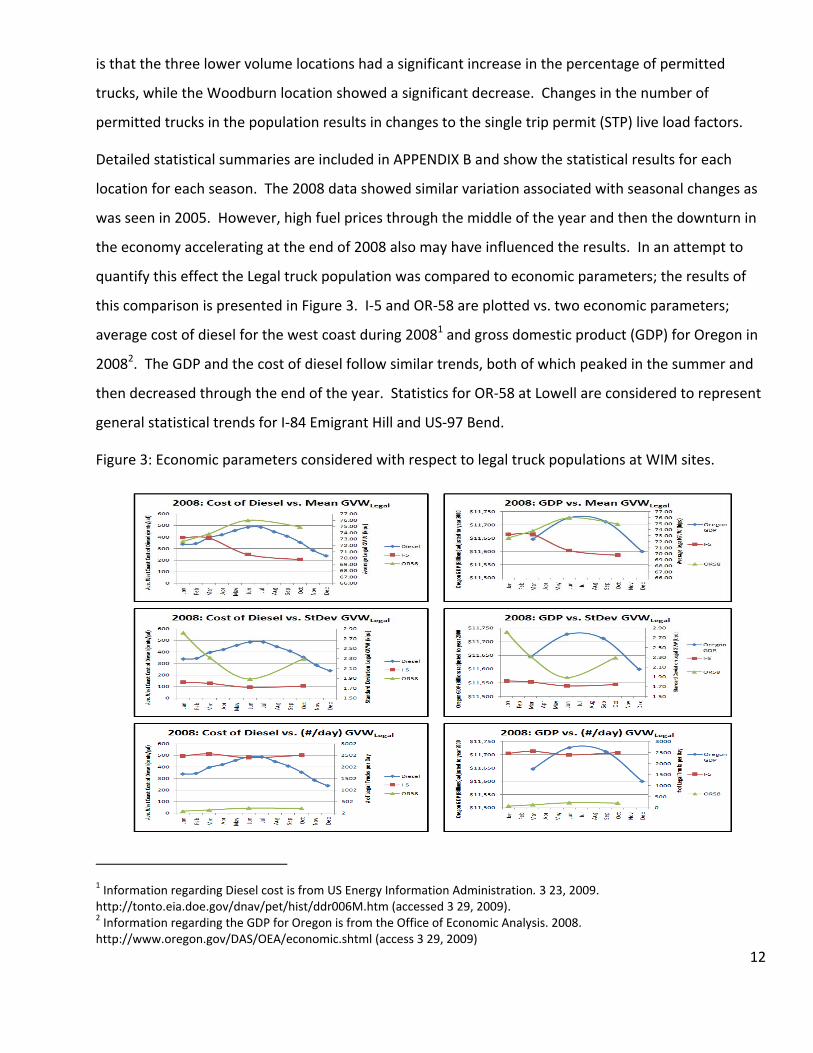
Detailed statistical summaries are included in APPENDIX B and show the statistical results for each

location for each season. The 2008 data showed similar variation associated with seasonal changes as

was seen in 2005. However, high fuel prices through the middle of the year and then the downturn in

the economy accelerating at the end of 2008 also may have influenced the results. In an attempt to

quantify this effect the Legal truck population was compared to economic parameters; the results of

this comparison is presented in Figure 3. I‐5 and OR‐58 are plotted vs. two economic parameters;

average cost of diesel for the west coast during 20081 and gross domestic product (GDP) for Oregon in

20082. The GDP and the cost of diesel follow similar trends, both of which peaked in the summer and

then decreased through the end of the year. Statistics for OR‐58 at Lowell are considered to represent

general statistical trends for I‐84 Emigrant Hill and US‐97 Bend.

Figure 3: Economic parameters considered with respect to legal truck populations at WIM sites.

1 Information regarding Diesel cost is from US Energy Information Administration. 3 23, 2009. http://tonto.eia.doe.gov/dnav/pet/hist/ddr006M.htm (accessed 3 29, 2009). 2 Information regarding the GDP for Oregon is from the Office of Economic Analysis. 2008. http://www.oregon.gov/DAS/OEA/economic.shtml (access 3 29, 2009)

13

Table 6: 2008 WIM Statistical Data

Data Tot. No No. of Mean Std. Dev COV Data Tot. No No. of Mean Std. Dev COV Data Tot. No No. of Mean Std. Dev COV

Classification Records Top 20% (Kips) (Kips) (%) Classification Records Top 20% (Kips) (Kips) (%) Classification Records Top 20% (Kips) (Kips) (%)

Table 1 (all) 126743 25349 71.91 2.70 4% Table 1 (all) 134852 26970 73.93 2.58 4% Table 1 (all) ‐6% ‐6% ‐3% 5% 7%

Table 1 (3S2 to 80k) 72843 14569 71.68 1.77 2% Table 1 (3S2 to 80k) 53997 10799 74.58 2.01 3% Table 1 (3S2 to 80k) 35% 35% ‐4% ‐12% ‐18%

Table 2 with CTP (all) 11724 2345 97.36 1.89 2% Table 2 with CTP (all) 14130 2826 101.74 1.71 2% Table 2 with CTP (all) ‐17% ‐17% ‐4% 11% ‐3%

Table 1 and 2 with CTP 138466 27693 80.17 8.94 11% Table 1 and 2 with CTP 148982 29797 83.37 9.70 12% Table 1 and 2 with CTP ‐7% ‐7% ‐4% ‐8% ‐5%

Table 3 No CTP 787 158 109.26 14.60 13% Table 3 No CTP 1947 389 91.04 17.40 19% Table 3 No CTP ‐60% ‐60% 20% ‐16% ‐31%

Table 4 110 22 150.61 16.30 11% Table 4 71 14 118.34 24.36 21% Table 4 55% 56% 27% ‐33% ‐47%

Table 5 7 2 144.30 #DIV/0! #DIV/0! Table 5 5 1 135.04 16.60 13% Table 5 35% 50% 7% #DIV/0! #DIV/0!

Table X 5 1 131.00 #DIV/0! #DIV/0! Table X 38 7 143.75 25.25 18% Table X ‐86% ‐86% ‐9% #DIV/0! #DIV/0!

Total Trucks 139375 Total Trucks 151042 Total Trucks ‐8%

Total Time (days) 29 Total Time (days) 31 Total Time (days) ‐4%

Recorded ADTT 4766 Recorded ADTT 4957 Recorded ADTT ‐4%

Suggested ADTT 5550 Suggested ADTT 5550 Suggested ADTT 0%

Total Permit Trucks 909 Total Permit Trucks 2060 Total Permit Trucks ‐56%

Permits/day 31 Permits/day 68 Permits/day ‐54%



Table 1 (all) 13372 2674 75.94 1.98 3% Table 1 (all) 14493 2899 75 2 0 Table 1 (all) ‐8% ‐8% 1% ‐2% ‐2%

Table 1 (3S2 to 80k) 6696 1339 77.97 1.09 1% Table 1 (3S2 to 80k) 7346 1469 77 1 0 Table 1 (3S2 to 80k) ‐9% ‐9% 1% ‐7% ‐8%

Table 2 with CTP (all) 1696 339 96.36 4.40 5% Table 2 with CTP (all) 1267 253 99 3 0 Table 2 with CTP (all) 34% 34% ‐3% 70% 81%

Table 1 and 2 with CTP 15067 3013 81.68 7.35 9% Table 1 and 2 with CTP 15760 3152 80 7 0 Table 1 and 2 with CTP ‐4% ‐4% 2% 0% ‐2%

Table 3 No CTP 401 80 109.97 11.04 10% Table 3 No CTP 363 73 86 18 0 Table 3 No CTP 11% 11% 28% ‐38% ‐52%

Table 4 13 3 169.94 8.75 5% Table 4 10 2 123 22 0 Table 4 33% 33% 38% ‐61% ‐71%

Table 5 6 1 139.01 #DIV/0! #DIV/0! Table 5 2 0 103 3 0 Table 5 260% 260% 35% #DIV/0! #DIV/0!

Table X 2 0 #DIV/0! #DIV/0! #DIV/0! Table X 11 4 113 14 0 Table X ‐86% ‐92% #DIV/0! #DIV/0! #DIV/0!



Recorded ADTT 550 Recorded ADTT 538 Recorded ADTT 2%


Total Permit Trucks 422 Total Permit Trucks 385 Total Permit Trucks 10%

Permits/day 15 Permits/day 13 Permits/day 18%

Data Tot. No No. of Mean Std. Dev COV Data Tot. No. of No. of Mean Std Dev COV Data Tot. No. of No. of Mean Std Dev COV

Classification Records Top 20% (Kips) (Kips) (%) Classification Records Top 20% (kips) (kips) (%) Classification Records Top 20% (kips) (kips) (%)

Table 1 (all) 9533 1907 73.54 2.59 4% Table 1 (all) 20653 4131 68.21 4.26 6% Table 1 (all) ‐54% ‐54% 8% ‐39% ‐44%

Table 1 (3S2) 5027 1005 74.35 2.33 5% Table 1 (3S2 to 80k) 10614 2123 66.13 3.12 5% Table 1 (3S2 to 80k) ‐53% ‐53% 12% ‐25% 0%

Table 2 with CTP (all) 1363 273 98.20 2.17 2% Table 2 with CTP (all) 832 166 92.08 2.42 3% Table 2 with CTP (all) 64% 64% 7% ‐10% ‐20%

Table 1 and 2 with CTP 10894 2179 84.26 8.04 10% Table 1 and 2 with CTP 21485 4297 72.08 7.58 11% Table 1 and 2 with CTP ‐49% ‐49% 17% 6% ‐10%Table 3 No CTP 385 77 106.86 5.33 5% Table 3 No CTP 38 8 95.53 20.43 21% Table 3 No CTP 919% 919% 12% ‐74% ‐77%

Table 4 38 8 143.10 23.83 16% Table 4 7 1 125.93 22.65 17% Table 4 467% 467% 14% 5% ‐6%

Table 5 5 1 154.23 #DIV/0! #DIV/0! Table 5 1 0 61.60 0.00 0% Table 5 800% 800% 150% #DIV/0! #DIV/0!

Table X 3 1 145.35 #DIV/0! #DIV/0! Table X 4 1 70.60 #DIV/0! #DIV/0! Table X ‐31% ‐45% 106% #DIV/0! #DIV/0!


Total Time (days) 31 Total Time (days) 30 Total Time (days) 3%







Table 1 (all) 36558 7312 74.50 2.14 3% Table 1 (all) 43550 8710 70.18 4.02 6% Table 1 (all) ‐16% ‐16% 6% ‐47% ‐51%

Table 1 (3S2 to 80k) 25610 5122 76.40 1.66 2% Table 1 (3S2 to 80k) 28633 5727 68.38 2.29 3% Table 1 (3S2 to 80k) ‐11% ‐11% 12% ‐28% ‐36%

Table 2 with CTP (all) 6383 1277 97.24 3.87 4% Table 2 with CTP (all) 4314 863 96.75 2.63 3% Table 2 with CTP (all) 48% 48% 1% 47% 48%

Table 1 and 2 with CTP 42940 8588 81.97 7.53 9% Table 1 and 2 with CTP 47864 9573 78.00 9.13 12% Table 1 and 2 with CTP ‐10% ‐10% 5% ‐18% ‐22%

Table 3 No CTP 2981 596 113.68 5.02 4% Table 3 No CTP 1012 202 93.90 18.27 20% Table 3 No CTP 195% 195% 21% ‐73% ‐78%

Table 4 64 13 149.28 15.31 10% Table 4 22 4 77.33 10.41 10% Table 4 192% 192% 93% 47% 6%

Table 5 18 4 118.63 8.07 6% Table 5 1 0 40.28 9.72 6% Table 5 3550% 3550% 195% ‐17% 4%

Table X 29 6 123.09 13.66 10% Table X 22 4 83.51 4.99 4% Table X 33% 34% 47% 174% 154%







Permits

per 1000

Trucks

211%

Permits

per 1000

Trucks

67.2

Permits

per 1000

Trucks

21.6

Permits

per 1000

Trucks

38

GVW Statistical Data for I‐84 E.Hill 2008 Annual Average GVW Statistical Data for I‐84 E.Hill 2005 Annual Average GVW Statistical Data for I‐84 E.Hill % Change

ADTT Verification ADTT Verification ADTT Verification

Permits

per 1000

Trucks

1236%

Permits

per 1000

Trucks

3

Permits

per 1000

Trucks

‐52%

GVW Statistical Data for OR‐58 Lowell 2008 Annual Average GVW Statistical Data for Lowell WB Annual Average 2005 GVW Statistical Data for Lowell WB % Change


Permits

per 1000

Trucks

27.2

Permits

per 1000

Trucks

23.8

Permits

per 1000

Trucks

14%

GVW Statistical Data for US‐97 Bend NB 2008 Annual Average GVW Statistical Data for US‐97 Bend NB 2005 Annual Average GVW Statistical Data for US‐97 Bend % Change


Permits

per 1000

Trucks

13.6

Permits

per 1000

Trucks

6.5

GVW Statistical Data for I5 Woodburn NB 2008 Annual Average GVW Statistical Data for I5 Woodburn NB 2005 Annual Average GVW Statistical Data for I5 Woodburn NB % Change


14

Figure 4: Statistical comparison GVW of legal truck populations at four WIM sites considered.

The observed changes in the truck population, regardless of cause, resulted in changes of the live load

factors as shown in the subsequent section.

Live Load Factors

LRFR live load factors for state‐owned bridges were calculated from the statistical data show in

Appendix B following the procedure outlined in the ODOT Policy Report. The maximum value for each

site at any season during 2008 is shown in Table 8. Comparison results from the 2005 calibration are

shown in Table 9 and the factors currently used by ODOT can be referred back to Table 1. As seen in

these tables, the live load factors for locations with ADTT greater than 5000 decreased, while the low

ADTT volume sites saw an increase in truck live load factors. The intermediate ADTT value site

remained about the same. The low volume site was controlled by Lowell and the resulting live load

factors are now larger than those now used in ODOT practice for the legal loads, CTP‐3, CTP‐2A and

CTP‐2B, as well as STP‐3, STP‐4A and STP‐5A. Detailed plots showing live load factor for each site,

rating vehicle, and seasonal variation are included in Appendix C.

0.50

1.00

1.50

2.00

2.50

3.00

3.50

4.00

60.00

62.00

64.00

66.00

68.00

70.00

72.00

74.00

76.00

78.00

80.00


Std. D

ev. Legal G

VW (kips)

Mean

Legal G

VW (kips)

I‐5 WBNB Statistical Data Comparison

2008 Mean

2005 Mean

2008 Std. Dev.

2005 Std. Dev.

0.50

1.00

1.50

2.00

2.50

3.00

3.50

4.00

60.00

62.00

64.00

66.00

68.00

70.00

72.00

74.00

76.00

78.00

80.00


Std. D

ev. Legal G

VW (kips)

Mean

Legal G

VW (kips)

Bend Statistical Data Comparison

2008 Mean

2005 Mean

2008 Std. Dev.

2005 Std. Dev.

0.50

1.00

1.50

2.00

2.50

3.00

3.50

4.00

60.00

62.00

64.00

66.00

68.00

70.00

72.00

74.00

76.00

78.00

80.00


Std. D

ev. Legal G

VW (kips)

Mean

Legal G

VW (kips)

Lowell Statistical Data Comparison

2008 Mean

2005 Mean

2008 Std. Dev.

2005 Std. Dev.

0.50

1.00

1.50

2.00

2.50

3.00

3.50

4.00

60.00

62.00

64.00

66.00

68.00

70.00

72.00

74.00

76.00

78.00

80.00


Std. D

ev. Legal G

VW (kips)

Mean

Legal G

VW (kips)

Emigrant Hill Stat Data Comparison

2008 Mean

2005 Mean

2008 Std. Dev.

2005 Std. Dev.

15

Table 7: 2008 Truck live load factors for different ADTT with controlling WIM site and month.

Table 8: Truck live load factors from 2005 WIM data.

≥ 5000 1500 ≤ 500 ≤ 500*

Legal Loads 1.36 WBNB Jan 1.34 EHill Jun‐Oct 1.34 Lowell Mar 1.33 Lowell Mar

CTP‐3 1.39 WBNB Jan 1.34 EHill Jun‐Oct 1.32 Lowell Mar 1.30 Lowell Mar

CTP‐2A, CTP‐2B 1.33 WBNB Jan 1.28 EHill Jun‐Oct 1.26 Lowell Mar 1.25 Lowell Mar

STP‐3 1.19 WBNB Jan 1.19 EHill Oct 1.15 Lowell Jun‐Oct 1.15 Lowell Jun‐Oct

STP‐4A 1.33 WBNB Jan 1.33 EHill Oct 1.28 Lowell Jun‐Oct 1.28 Lowell Jun‐Oct

STP‐4B 0.96 WBNB Jan 0.96 EHill Jun‐Oct 0.94 Lowell Oct 0.94 Lowell Oct

STP‐5A 1.06 WBNB Jan 1.06 EHill Jun‐Oct 1.03 Lowell Jun‐Oct 1.03 Lowell Jun‐Oct

STP‐5B 1.02 WBNB Jan 1.02 EHill Jun‐Oct 0.99 Lowell Mar‐Jun‐Oct 0.99 Lowell Mar‐Jun‐Oct

STP‐5C 0.84 WBNB Jan 0.84 EHill Jun‐Oct 0.82 Bend Jan Lowell Mar‐Jun‐Oct 0.82 Bend Jan Lowell Mar‐Jun‐Oct

STP‐5BW 0.92 WBNB Jan 0.93 EHill Oct 0.90 Lowell Jun‐Oct 0.90 Lowell Jun‐Oct

UPPERBOUND 2008

Note: WBNB=Woodburn NB and EHill=Emigrant Hill.

* indicates calculations performed using average annual recorded 2008 WIM ADTT for Lowell (ADTT = 370)

ADTT

≥ 5000 1500 ≤ 500

Legal Loads 1.40 1.34 1.30

CTP‐3 1.43 1.39 1.29

CTP‐2A, CTP‐2B 1.36 1.33 1.24

STP‐3 1.23 1.18 1.11

STP‐4A 1.38 1.32 1.24

STP‐4B 0.99 0.96 0.91

STP‐5A 1.09 1.06 1.00

STP‐5B 1.05 1.02 0.97

STP‐5C 0.86 0.84 0.81

STP‐5BW 0.95 0.92 0.88

UPPERBOUND

2005

ADTT

16

Table 9: Percent change in truck live load factor for high, moderate, and low volume sites.

Figure 5: Live load factor comparisons for high, moderate, and low volume sites.

≥ 5000 1500 ≤ 500

Legal Loads ‐3% 0% 3%

CTP‐3 ‐3% ‐4% 2%

CTP‐2A, CTP‐2B ‐2% ‐4% 2%

STP‐3 ‐4% 1% 4%

STP‐4A ‐4% 1% 3%

STP‐4B ‐3% 0% 3%

STP‐5A ‐3% 0% 3%

STP‐5B ‐3% 0% 2%

STP‐5C ‐2% 0% 2%

STP‐5BW ‐3% 1% 2%

ADTTUPPERBOUND

% Change

17

As seen in Table 7, compared to 2005 results in Table 8, the Lowell site produced higher live load

factors for almost all truck types. Referencing Table 5, the WIM recorded average ADTT is substantially

less than the corresponding 2005 values. The Lowell live load factors were recalculated using a WIM

measured average ADTT value of 370 (the recorded average for 2008). The resulting change in live

load factors are shown in the far right column of Table 7 and were slightly smaller.

The same approach to rounding live load factors established by Groff (2006) was applied to the low

volume site. Table 10 shows the resulting live load factors if the Lowell ADTT = 581, while Table 11

shows the resulting live load factors if the Lowell ADTT = 370.

Table 10: Rounded Live Load Factor Comparison w/ Lowell ADTT = 581

Table 11: Rounded Live Load Factor Comparison w/ Lowell ADTT = 370

ADTT ≤ 500 w/

Lowell ADTT = 581

ODOT

Current

Actual

2008

Rounded

08% Change

Legal Loads 1.30 1.34 1.35 4%

CTP‐3 1.30 1.32 1.35 4%

CTP‐2A, CTP‐2B 1.25 1.26 1.30 4%

STP‐3 1.10 1.15 1.15 5%

STP‐4A 1.25 1.28 1.30 4%

STP‐4B 1.00 0.94 1.00 0%

STP‐ 5A 1.00 1.03 1.05 5%

STP‐5B 1.00 0.99 1.00 0%

STP‐5C 1.00 0.82 1.00 0%

STP‐5BW 1.00 0.90 1.00 0%

ADTT ≤ 500 w/

Lowell ADTT = 370

ODOT

Current

Actual

2008

Rounded

08% Change

Legal Loads 1.30 1.32 1.35 4%

CTP‐3 1.30 1.30 1.30 0%

CTP‐2A, CTP‐2B 1.25 1.25 1.25 0%

STP‐3 1.10 1.15 1.15 5%

STP‐4A 1.25 1.28 1.30 4%

STP‐4B 1.00 0.94 1.00 0%

STP‐ 5A 1.00 1.03 1.05 5%

STP‐5B 1.00 0.99 1.00 0%

STP‐5C 1.00 0.82 1.00 0%

STP‐5BW 1.00 0.90 1.00 0%

18

Conclusion and Recommendations

Based on recalculation of the Oregon‐specific live load factors, using 2008 WIM data, for four sites, and

four months in different seasons, and compared with prior 2005 results, the following conclusions and

recommendations are presented:

WIM records for I5 at Woodburn in 2008 compared to 2005, showed fewer trucks with lighter

legal loads, resulting in smaller truck live load factors for the high volume location.

WIM records for I84 at Emigrant Hill in 2008 compared to 2005, showed less seasonal variation

but similar peak effects, resulting in similar live load factors for the intermediate volume site.

WIM records for US97 at Bend in 2008 compared to 2005, showed little change with respect to

2005 values.

WIM records for OR58 at Lowell in 2008 compared to 2005, showed significantly fewer trucks

(nearly 50%). At the same time, the mean gross vehicle weights increased by the largest

margin, which resulted in higher live load factors. Lowell controlled the low volume sites live

load factor selection in all cases.

If Lowell is taken to represent sites with ADTT < 500 then the low volume site live load factors

should be increased, unless there is a unique operational rationale (construction routing for

example) to account for the observed changes. As was shown in Table 10 and Table 11, the

selection of the ADTT value for this site should be taken into consideration when choosing the

final live load factors.

Based on the economic conditions and diesel fuel price variation, 2008 may be an atypical year

with respect to the truck populations in Oregon.

Given the changes observed at the low volume site, it is recommended that the live load factors

be recalculated when the economic and/or diesel fuel pricing conditions change, regardless of

the time increment since the last calculation. Thresholds for these changes are not known at

this time. Recalculation is also recommended if policy changes would in turn alter the truck

population characteristics.

WIM data should continue to be collected and archived by ODOT to facilitate future data

analysis.

19

Works Cited/Consulted

Administration, U. E. (2009, 3 23). Energy Information Administration. Retrieved 3 29, 2009, from

http://tonto.eia.doe.gov/dnav/pet/hist/ddr006M.htm

Groff, R. L. (2006). ODOT LRFR POLICY REPORT: LIVELOAD FACTORS FOR USE IN LOAD AND RESISTANCE

FACTOR RATING (LRFR) OF OREGON'S STATE‐OWNED BRIDGES. Oregon Department of

Transportation.

Office of Economic Analysis. (2008). Retrieved 3 28, 2009, from Oregon.gov:

http://www.oregon.gov/DAS/OEA/economic.shtml

Pelphrey, J., Higgins, C., Sivakumar, B., Groff, R., Hartman, B., Charbonneau, J., Rooper, J., and Johnson,

B. (2008). State‐Specific LRFR Live Load Factors Using Weigh‐in‐Motion Data. Journal of Bridge

Engineering, July/August, 339‐350.

Pelphrey, J., & Higgins, C. (2006). CALIBRATION OF LRFR LIVE LOAD FACTORS USING WEIGH‐IN‐MOTION

DATA. Corvallis: Oregon State University.

Moses, F. (2001). NCHRP REPORT 454: Calibration of Load Factors for LRFR Bridge Evaluation.

Washington, D.C.: National Academy Press.

Sivakumar, B. (2005). CALIBRATION OF LRFR LIVE LOAD FACTORS FOR OREGON USING I‐5 WEIGH‐IN‐

MOTION DATA. New Jersey: Lichtenstein Consulting Engineers, Inc.

LRFR Manual (2008). ODOT LRFR Manual. ODOT.

20

APPENDIX A: Permit Weight Tables

Figure 6: Permit Weight Table 1

21

Figure 7: Permit Weight Table 2

22

Figure 8: Permit Weight Table 3 (1/2)

23


24


25


26


27

Figure 13: Permit Weight Table (2/2)

28

APPENDIX B: Statistical Data

Table 12: Lowell GVW Statistical Data 2008

Data Tot. No No. of Mean Std. Dev COV Data Tot. No. of No. of Mean Std Dev COV Data Tot. No No. of Mean Std. Dev COV

Classification Records Top 20% (Kips) (Kips) (%) Classification Records Top 20% (kips) (kips) (%) Classification Records Top 20% (Kips) (Kips) (%)

Table 1 (all) 5611 1122.2 72.81 3.18 4.36% Table 1 (all) 15157 3031 66.56 5.06 8% Table 1 (all) ‐63% ‐63% 9% ‐37% ‐43%

Table 1 (3S2) 2606 521.2 72.64 2.82 10.34% Table 1 (3S2 to 80k) 7373 1475 62.79 3.61 6% Table 1 (3S2) ‐65% ‐65% 16% ‐22% 80%

Table 2 with CTP (all) 1164 232.8 97.14 2.03 2.09% Table 2 with CTP (all) 473 95 89.00 2.96 3% Table 2 with CTP (all) 146% 146% 9% ‐31% ‐37%

Table 1 and 2 with CTP 6775 1355 87.74 6.83 7.78% Table 1 and 2 with CTP 15630 3126 70.02 7.45 11% Table 1 and 2 with CTP ‐57% ‐57% 25% ‐8% ‐27%

Table 3 No CTP 237 47.4 102.43 2.29 2.24% Table 3 No CTP 26 5 96.00 19.41 20% Table 3 No CTP 812% 812% 7% ‐88% ‐89%

Table 4 18 3.6 149.45 30.09 20.14% Table 4 3 1 129.03 37.82 29% Table 4 500% 500% 16% ‐20% ‐31%

Table 5 1 0.2 158.00 #DIV/0! #DIV/0! Table 5 0 0 Table 5 #DIV/0! #DIV/0! #DIV/0! #DIV/0! #DIV/0!

Table X 2 0.4 138.80 #DIV/0! #DIV/0! Table X 0 0 0.00 0.00 0.00% Table X #DIV/0! #DIV/0! #DIV/0! #DIV/0! #DIV/0!

Total Trucks 7033 Total Trucks 15659 Total Trucks 23343%





Permits/day 9 Permits/day 1 Permits/day #REF!



Table 1 (all) 7965 1593 73.31 2.53 3.46% Table 1 (all) 17455 3491 66.94 4.71 7% Table 1 (all) ‐54% ‐54% 10% ‐46% ‐51%

Table 1 (3S2) 4253 850.6 73.84 2.32 3.14% Table 1 (3S2 to 80k) 9103 1821 63.69 2.99 5% Table 1 (3S2) ‐53% ‐53% 16% ‐22% ‐33%

Table 2 with CTP (all) 1257 251.4 97.66 2.29 2.34% Table 2 with CTP (all) 436 87 88.46 2.01 2% Table 2 with CTP (all) 188% 188% 10% 14% 3%

Table 1 and 2 with CTP 9222 1844.4 85.25 8.40 9.85% Table 1 and 2 with CTP 17891 3578 69.57 6.89 10% Table 1 and 2 with CTP ‐48% ‐48% 23% 22% ‐1%


Table 4 19 3.8 133.00 4.24 3.19% Table 4 3 1 108.60 4.20 4% Table 4 533% 533% 22% 1% ‐18%

Table 5 4 0.8 139.80 #DIV/0! #DIV/0! Table 5 0 0 Table 5 #DIV/0! #DIV/0! #DIV/0! #DIV/0! #DIV/0!

Table X 1 0.2 95.30 #DIV/0! #DIV/0! Table X 0 0 0.00 #DIV/0! #DIV/0! Table X #DIV/0! #DIV/0! #DIV/0! #DIV/0! #DIV/0!










Table 1 (3S2) 6716 1343.2 75.99 1.89 2.48% Table 1 (3S2 to 80k) 12842 2568 67.41 3.14 5% Table 1 (3S2) ‐48% ‐48% 13% ‐40% ‐47%

Table 2 with CTP (all) 1593 318.6 98.93 2.18 2.20% Table 2 with CTP (all) 999 200 94.86 2.29 2% Table 2 with CTP (all) 59% 59% 4% ‐5% ‐9%

Table 1 and 2 with CTP 14096 2819.2 82.04 8.34 10.17% Table 1 and 2 with CTP 25764 5153 72.91 7.99 11% Table 1 and 2 with CTP ‐45% ‐45% 13% 4% ‐7%


Table 4 79 15.8 139.45 31.34 22.47% Table 4 12 2 127.71 26.31 21% Table 4 558% 558% 9% 19% 9%

Table 5 7 1.4 195.50 20.22 10.34% Table 5 1 0 138.10 Table 5 600% 600% 42% #DIV/0! #DIV/0!

Table X 6 1.2 204.00 3.96 1.94% Table X 3 1 114.60 0.00 0.00% Table X #DIV/0! 20% 78% #DIV/0! #DIV/0!









Table 1 (all) 12051 2410.2 73.71 2.44 3.31% Table 1 (all) 25235 5047 70.62 3.33 5.00% Table 1 (all) ‐52% ‐52% 4% ‐27% ‐34%

Table 1 (3S2) 6533 1306.6 74.95 2.29 3.06% Table 1 (3S2) 13138 2628 70.64 2.74 4.00% Table 1 (3S2) ‐50% ‐50% 6% ‐16% ‐24%

Table 2 with CTP (all) 1438 287.6 99.07 2.18 2.20% Table 2 with CTP (all) 1419 284 95.99 2.40 3.00% Table 2 with CTP (all) 1% 1% 3% ‐9% ‐27%

Table 1 and 2 with CTP 13484 2696.8 81.99 8.59 10.47% Table 1 and 2 with CTP 26654 5331 75.84 7.99 11.00% Table 1 and 2 with CTP ‐49% ‐49% 8% 7% ‐5%

Table 3 No CTP 485 97 110.31 8.83 8.00% Table 3 No CTP 61 12 97.70 22.41 23.00% Table 3 No CTP 695% 695% 13% ‐61% ‐65%

Table 4 37 7.4 150.49 29.65 19.71% Table 4 9 2 138.38 22.28 16.00% Table 4 311% 311% 9% 33% 23%

Table 5 6 1.2 123.60 2.97 2.40% Table 5 1 0 108.30 Table 5 500% 500% 14% #DIV/0! #DIV/0!

Table X 2 0.4 143.30 #DIV/0! #DIV/0! Table X 13 3 167.80 18.35 10.94% Table X ‐85% ‐87% ‐15% #DIV/0! #DIV/0!







GVW Statistical Data for Lowell WB WIM Record - June 2005

% Change GVW Statistical Data for Lowell WB January

ADTT Verification

% Change GVW Statistical Data for Lowell WB March

ADTT Verification

% Change GVW Statistical Data for Lowell WB June

GVW Statistical Data for Lowell October 08

ADTT Verification

ADTT Verification

GVW Statistical Data for Lowell June 08

ADTT Verification

GVW Statistical Data for OR‐58 Lowell January

ADTT Verification

GVW Statistical Data for OR‐58 Lowell March 08

ADTT Verification

% Change GVW Statistical Data for Lowell WB October

ADTT Verification

GVW Statistical Data for Lowell October 05

ADTT Verification

GVW Statistical Data for Lowell WB WIM Record ‐ January 2005

ADTT Verification

ADTT Verification

ADTT Verification

GVW Statistical Data for Lowell WB WIM Record ‐ April 2005

29

Table 13: Woodburn GVW Statistical data 2008



Table 1 (all) 128382 25677 73.21 2.39 3.26% Table 1 (all) 124062 24812 73.66 2.55 3.00% Table 1 (all) 3% 3% ‐1% ‐6% 9%

Table 1 (3S2 to 80k) 76543 15309 73.22 1.82 2.48% Table 1 (3S2 to 80k) 44167 8833 73.85 2.11 3.00% Table 1 (3S2) 73% 73% ‐1% ‐14% ‐17%

Table 2 with CTP (all) 13348 2670 99.38 1.85 1.86% Table 2 with CTP (all) 13652 2730 101.49 1.72 2.00% Table 2 with CTP (all) ‐2% ‐2% ‐2% 8% ‐7%

Table 1 and 2 with CTP 141730 28346 82.30 9.19 11.16% Table 1 and 2 with CTP 137714 27543 83.85 9.84 12.00% Table 1 and 2 with CTP 3% 3% ‐2% ‐7% ‐7%

Table 3 No CTP 1123 225 108.18 11.94 11.04% Table 3 No CTP 1311 262 89.29 17.75 20.00% Table 3 No CTP ‐14% ‐14% 21% ‐33% ‐45%

Table 4 219 44 140.54 18.90 13.45% Table 4 44 9 118.09 21.46 18.00% Table 4 398% 400% 19% ‐12% ‐25%

Table 5 12 3 164.37 13.26 8.07% Table 5 1 0 152.30 Table 5 1100% 1400% 8% #DIV/0! #DIV/0!

Table X 10 2 125.35 38.68 30.86% Table X 32 6 145.89 23.98 16.44% Table X ‐69% ‐69% ‐14% 61% 88%









Table 1 (all) 136073 27214.6 73.09 2.42 3.31% Table 1 (all) 136363 27273 73.60 2.58 4.00% Table 1 (all) 0% 0% ‐1% ‐6% ‐17%

Table 1 (3S2) 79470 15894 73.19 1.80 2.46% Table 1 (3S2) 49232 9846 74.04 2.05 3.00% Table 1 (3S2) 61% 61% ‐1% ‐12% ‐18%

Table 2 with CTP (all) 13165 2633 99.39 1.96 1.97% Table 2 with CTP (all) 13675 2735 101.43 1.72 2.00% Table 2 with CTP (all) ‐4% ‐4% ‐2% 14% ‐1%

Table 1 and 2 with CTP 149238 29847.6 81.61 9.11 11.16% Table 1 and 2 with CTP 150038 30008 83.05 9.81 12.00% Table 1 and 2 with CTP ‐1% ‐1% ‐2% ‐7% ‐7%

Table 3 No CTP 1009 201.8 106.61 8.37 7.85% Table 3 No CTP 1226 245 90.40 19.01 21.00% Table 3 No CTP ‐18% ‐18% 18% ‐56% ‐63%

Table 4 74 14.8 143.40 12.57 8.77% Table 4 57 11 127.66 30.47 24.00% Table 4 30% 30% 12% ‐59% ‐63%

Table 5 8 1.6 122.25 36.13 29.56% Table 5 1 0 134.10 Table 5 700% 700% ‐9% #DIV/0! #DIV/0!

Table X 6 1.2 108.45 19.30 17.80% Table X 25 5 137.10 24.16 17.62% Table X ‐76% ‐76% ‐21% ‐20% 1%









Table 1 (all) 106078 21216 70.94 2.89 4.08% Table 1 (all) 143018 28604 74.41 2.54 3.00% Table 1 (all) ‐26% ‐26% ‐5% 14% 36%

Table 1 (3S2) 57707 11541 70.55 1.72 2.43% Table 1 (3S2) 58455 11691 75.48 1.90 3.00% Table 1 (3S2) ‐1% ‐1% ‐7% ‐10% ‐19%

Table 2 with CTP (all) 7903 1581 95.48 2.08 2.18% Table 2 with CTP (all) 15622 3124 102.18 1.67 2.00% Table 2 with CTP (all) ‐49% ‐49% ‐7% 24% 9%

Table 1 and 2 with CTP 113981 22796 77.78 8.48 10.90% Table 1 and 2 with CTP 158640 31728 83.72 9.61 11.00% Table 1 and 2 with CTP ‐28% ‐28% ‐7% ‐12% ‐1%

Table 3 No CTP 572 114 107.79 17.15 15.92% Table 3 No CTP 2775 555 92.00 16.53 18.00% Table 3 No CTP ‐79% ‐79% 17% 4% ‐12%

Table 4 65 13 164.83 22.48 13.64% Table 4 89 18 115.03 20.98 18.00% Table 4 ‐27% ‐27% 43% 7% ‐24%

Table 5 3 1 179.70 #DIV/0! #DIV/0! Table 5 4 1 127.38 36.94 29.00% Table 5 ‐25% ‐25% 41% #DIV/0! #DIV/0!

Table X 1 0 146.70 #DIV/0! #DIV/0! Table X 47 9 145.30 21.37 14.71% Table X ‐98% ‐98% 1% #DIV/0! #DIV/0!



Recorded ADTT 4776 Recorded ADTT 5385.1667 Recorded ADTT ‐11%






Table 1 (all) 136437 27287.4 70.40 3.10 4.40% Table 1 (all) 135964 27193 74.03 2.64 4.00% Table 1 (all) 0% 0% ‐5% 17% 10%

Table 1 (3S2) 77653 15530.6 69.76 1.74 2.50% Table 1 (3S2) 64133 12827 74.93 1.97 3.00% Table 1 (3S2) 21% 21% ‐7% ‐12% ‐17%

Table 2 with CTP (all) 12478 2495.6 95.19 1.69 1.78% Table 2 with CTP (all) 13572 2714 101.87 1.74 2.00% Table 2 with CTP (all) ‐8% ‐8% ‐7% ‐3% ‐11%

Table 1 and 2 with CTP 148915 29783 78.97 8.99 11.39% Table 1 and 2 with CTP 149536 29907 82.87 9.53 12.00% Table 1 and 2 with CTP 0% 0% ‐5% ‐6% ‐5%

Table 3 No CTP 445 89 114.47 20.91 18.27% Table 3 No CTP 2476 495 92.46 16.30 18.00% Table 3 No CTP ‐82% ‐82% 24% 28% 1%

Table 4 82 16.4 153.66 11.25 7.32% Table 4 93 19 112.59 24.51 22.00% Table 4 ‐12% ‐12% 36% ‐54% ‐67%

Table 5 4 0.8 110.90 #DIV/0! #DIV/0! Table 5 14 3 126.38 29.46 23.00% Table 5 ‐71% ‐71% ‐12% #DIV/0! #DIV/0!

Table X 4 0.8 143.50 #DIV/0! #DIV/0! Table X 46 9 146.72 31.49 21.46% Table X ‐91% ‐91% ‐2% #DIV/0! #DIV/0!







GVW Statistical Data for I5 Woodburn NB October 08

GVW Statistical Data for I5 Woodburn NB January 2008

ADTT Verification

ADTT Verification

GVW Statistical Data for I‐5 Woodburn NB March 08

ADTT Verification

GVW Statistical Data for I‐5 Woodburn NB April 05

ADTT Verification

% Change GVW Statistical Data for I5 Woodburn NB June

ADTT Verification

% Change GVW Statistical Data for I5 Woodburn NB April

GVW Statistical Data for I5 Woodburn NB January 2005

GVW Statistical Data for I5 Woodburn NB June 05

ADTT Verification

GVW Statistical Data for I5 Woodburn NB June 08

ADTT Verification

ADTT Verification

% Change GVW Statistical Data for I5 Woodburn NB June

ADTT Verification

ADTT Verification

GVW Statistical Data for I5 Woodburn NB October 05

ADTT Verification

% Change GVW Statistical Data for I5 Woodburn NB October

ADTT Verification

30

Table 14: Bend GVW Statistical Data 2008


Classification Records Top 20% (Kips) end (%) Classification Records Top 20% (Kips) (Kips) (%) Classification Records Top 20% (Kips) (Kips) (%)

Table 1 (all) 10654 2130.8 75.99 1.95 2.57% Table 1 (all) 9776 1955.2 75.59 1.78 2% Table 1 (all) 9% 9% 1% 9% 9%

Table 1 (3S2 to 80k) 5865 1173 77.74 1.32 1.70% Table 1 (3S2 to 80k) 5305 1061 76.52 1.30 2% Table 1 (3S2 to 80k) 11% 11% 2% 2% 0%

Table 2 with CTP (all) 1270 254 102.00 1.85 1.81% Table 2 with CTP (all) 596 119.2 101.12 1.40 1% Table 2 with CTP (all) 113% 113% 1% 32% 31%

Table 1 and 2 with CTP 11924 2384.8 82.65 8.44 10.21% Table 1 and 2 with CTP 10372 2074.4 80.21 8.02 10% Table 1 and 2 with CTP 15% 15% 3% 5% 2%

Table 3 No CTP 322 64.4 109.56 13.14 12.00% Table 3 No CTP 213 42.6 85.26 18.47 22% Table 3 No CTP 51% 51% 29% ‐29% ‐45%

Table 4 7 1.4 164.45 0.92 0.56% Table 4 9 1.8 110.48 11.19 10% Table 4 ‐22% ‐22% 49% ‐92% ‐94%

Table 5 7 1.4 74.15 13.08 17.64% Table 5 0 0 Table 5 #DIV/0! #DIV/0! #DIV/0! #DIV/0! #DIV/0!

Table X 0 0 #DIV/0! #DIV/0! #DIV/0! Table X 1 0 75.30 0.00 0.00% Table X ‐100% #DIV/0! #DIV/0! #DIV/0! #DIV/0!









Table 1 (all) 12766 2553.2 76.46 1.83 2.39% Table 1 (all) Table 1 (all) #DIV/0! #DIV/0! #DIV/0! #DIV/0! #DIV/0!

Table 1 (3S2) 6776 1355.2 78.39 0.93 1.18% Table 1 (3S2) Table 1 (3S2 to 80k) #DIV/0! #DIV/0! #DIV/0! #DIV/0! #DIV/0!

Table 2 with CTP (all) 2260 452 97.28 5.22 5.36% Table 2 with CTP (all) Table 2 with CTP (all) #DIV/0! #DIV/0! #DIV/0! #DIV/0! #DIV/0!

Table 1 and 2 with CTP 15026 3005.2 82.38 6.81 8.27% Table 1 and 2 with CTP Table 1 and 2 with CTP #DIV/0! #DIV/0! #DIV/0! #DIV/0! #DIV/0!

Table 3 No CTP 599 119.8 107.84 5.01 4.65% Table 3 No CTP Table 3 No CTP #DIV/0! #DIV/0! #DIV/0! #DIV/0! #DIV/0!

Table 4 8 1.6 179.10 5.09 2.84% Table 4 Table 4 #DIV/0! #DIV/0! #DIV/0! #DIV/0! #DIV/0!

Table 5 7 1.4 183.10 6.65 3.63% Table 5 Table 5 #DIV/0! #DIV/0! #DIV/0! #DIV/0! #DIV/0!

Table X 1 0.2 65.60 #DIV/0! #DIV/0! Table X Table X #DIV/0! #DIV/0! #DIV/0! #DIV/0! #DIV/0!

Total Trucks 15641 Total Trucks Total Trucks #DIV/0!

Total Time (days) 31 Total Time (days) Total Time (days) #DIV/0!

Recorded ADTT 505 Recorded ADTT Recorded ADTT #DIV/0!

Suggested ADTT 607 Suggested ADTT Suggested ADTT #DIV/0!

Total Permit Trucks 615 Total Permit Trucks Total Permit Trucks #DIV/0!

Permits/day 20 Permits/day Permits/day #DIV/0!



Table 1 (all) 12914 2582.8 75.32 2.39 3.18% Table 1 (all) 15676 3135 76.17 2.32 3% Table 1 (all) ‐18% ‐18% ‐1% 3% 4%

Table 1 (3S2) 5604 1120.8 78.08 1.06 1.36% Table 1 (3S2) 7605 1521 78.54 0.87 1% Table 1 (3S2 to 80k) ‐26% ‐26% ‐1% 22% 23%

Table 2 with CTP (all) 1637 327.4 85.19 7.97 9.36% Table 2 with CTP (all) 2379 476 97.20 4.84 5% Table 2 with CTP (all) ‐31% ‐31% ‐12% 65% 88%

Table 1 and 2 with CTP 14551 2910.2 80.82 6.75 8.35% Table 1 and 2 with CTP 18055 3611 81.76 6.46 8% Table 1 and 2 with CTP ‐19% ‐19% ‐1% 5% 6%

Table 3 No CTP 317 63.4 110.24 11.02 10.00% Table 3 No CTP 688 138 88.40 16.38 19% Table 3 No CTP ‐54% ‐54% 25% ‐33% ‐46%


Table 5 7 1.4 103.60 14.70 14.19% Table 5 1 0 176.00 0.00 0% Table 5 600% 600% ‐41% #DIV/0! #DIV/0!

Table X 3 0.6 190.80 #DIV/0! #DIV/0! Table X 20 9 157.48 33.55 21.30% Table X ‐85% ‐93% 21% #DIV/0! #DIV/0!










Table 1 (3S2) 8539 1707.8 77.67 1.07 1.37% Table 1 (3S2) 9129 1826 75.68 1.35 2% Table 1 (3S2 to 80k) ‐6% ‐6% 3% ‐21% ‐23%


Table 1 and 2 with CTP 18768 3753.6 80.87 7.40 9.16% Table 1 and 2 with CTP 18853 3771 78.79 7.57 10% Table 1 and 2 with CTP 0% 0% 3% ‐2% ‐5%



Table 5 3 0.6 195.20 #DIV/0! #DIV/0! Table 5 4 1 133.35 8.73 7% Table 5 ‐25% ‐25% 46% #DIV/0! #DIV/0!

Table X 2 0.4 130.50 #DIV/0! #DIV/0! Table X 11 2 105.50 8.77 8.31% Table X ‐82% ‐80% 24% #DIV/0! #DIV/0!


Total Time (days) 31 Total Time (days) 30 Total Time (days) #NAME?





ADTT Verification ADTT Verification

GVW Statistical Data for US‐97 Bend June 08 GVW Statistical Data for US‐97 Bend June 05


GVW Statistical Data for US‐97 Bend October 08 GVW Statistical Data for US‐97 Bend October 05


GVW Statistical Data for US‐97 Bend March 08 GVW Statistical Data for US‐97 Bend April 05


GVW Statistical Data for US‐97 Bend January 2008 GVW Statistical Data for US‐97 Bend December 2005

ADTT Verification

% Change GVW Statistical Data for US‐97 Bend Fall

ADTT Verification

% Change GVW Statistical Data for US‐97 Bend Winter

ADTT Verification

% Change GVW Statistical Data for US‐97 Bend Spring

ADTT Verification

% Change GVW Statistical Data for US‐97 Bend Summer

31

Table 15: Emigrant Hill GVW Statistical Data 2008


Classification Records Top 20% (Kips) end (%) Classification Records Top 20% (Kips) (Kips) (%) Classification Records Top 20% (Kips) (Kips) (%)

Table 1 (all) 24955 4991 74.41 2.38 3.20% Table 1 (all) 43416 8683 67.37 5.32 8% Table 1 (all) ‐43% ‐43% 10% ‐55% ‐60%

Table 1 (3S2 to 80k) 17588 3517.6 76.03 1.93 2.54% Table 1 (3S2 to 80k) 26657 5331 63.32 2.33 4% Table 1 (3S2 to 80k) ‐34% ‐34% 20% ‐17% ‐31%


Table 1 and 2 with CTP 28462 5692.4 80.44 6.19 7.69% Table 1 and 2 with CTP 45654 9131 73.18 9.33 13% Table 1 and 2 with CTP ‐38% ‐38% 10% ‐34% ‐40%

Table 3 No CTP 1715 343 112.07 5.31 4.74% Table 3 No CTP 58 12 86.30 19.41 22% Table 3 No CTP 2857% 2857% 30% ‐73% ‐79%

Table 4 32 6.4 140.24 21.28 15.17% Table 4 2 0 87.15 7.99 9% Table 4 1500% 1500% 61% 166% 66%

Table 5 11 2.2 105.40 1.40 1.33% Table 5 0 0 Table 5 #DIV/0! #DIV/0! #DIV/0! #DIV/0! #DIV/0!

Table X 33 6.6 119.64 10.29 8.60% Table X 0 0 0.00 0.00 0.00% Table X #DIV/0! #DIV/0! #DIV/0! #DIV/0! #DIV/0!









Table 1 (all) 36031 7206.2 74.74 2.18 2.92% Table 1 (all) 37249 7450 75.32 2.03 3% Table 1 (all) ‐3% ‐3% ‐1% 7% 8%

Table 1 (3S2) 25652 5130.4 77.18 1.46 1.89% Table 1 (3S2) 28021 5604 76.64 1.66 2% Table 1 (3S2 to 80k) ‐8% ‐8% 1% ‐12% ‐13%

Table 2 with CTP (all) 7485 1497 95.22 4.94 5.19% Table 2 with CTP (all) 7121 1424 98.92 3.54 4% Table 2 with CTP (all) 5% 5% ‐4% 40% 45%

Table 1 and 2 with CTP 43516 8703.2 82.00 6.82 8.32% Table 1 and 2 with CTP 44370 8874 83.87 7.82 9% Table 1 and 2 with CTP ‐2% ‐2% ‐2% ‐13% ‐11%

Table 3 No CTP 3398 679.6 114.03 4.01 3.51% Table 3 No CTP 3489 698 98.49 13.81 14% Table 3 No CTP ‐3% ‐3% 16% ‐71% ‐75%

Table 4 72 14.4 130.75 10.13 7.75% Table 4 73 15 115.65 23.35 20% Table 4 ‐1% ‐1% 13% ‐57% ‐62%

Table 5 24 4.8 117.34 3.04 2.59% Table 5 2 0 161.10 38.89 24% Table 5 1100% 1100% ‐27% ‐92% ‐89%

Table X 33 6.6 112.46 5.59 4.97% Table X 77 15 121.14 16.42 13.55% Table X ‐57% ‐56% ‐7% ‐66% ‐63%










Table 1 (3S2) 29875 5975 75.75 1.72 2.27% Table 1 (3S2) 30429 6086 70.30 2.85 4% Table 1 (3S2 to 80k) ‐2% ‐2% 8% ‐40% ‐44%


Table 1 and 2 with CTP 49968 9993.6 81.92 8.65 10.55% Table 1 and 2 with CTP 49911 9982 80.48 9.48 12% Table 1 and 2 with CTP 0% 0% 2% ‐9% ‐10%


Table 4 51 10.2 163.61 10.86 6.64% Table 4 13 3 106.53 10.32 10% Table 4 292% 292% 54% 5% ‐31%

Table 5 19 3.8 111.68 7.55 6.76% Table 5 0 0 0.00 0.00 0% Table 5 #DIV/0! #DIV/0! #DIV/0! #DIV/0! #DIV/0!

Table X 9 1.8 147.90 29.42 19.89% Table X 8 2 122.10 3.54 2.90% Table X 13% ‐10% 21% 731% 586%










Table 1 (3S2) 29325 5865 76.64 1.51 1.97% Table 1 (3S2) 29423 5885 63.25 2.33 4% Table 1 (3S2 to 80k) 0% 0% 21% ‐35% ‐47%


Table 1 and 2 with CTP 49814 9962.8 83.52 8.44 10.11% Table 1 and 2 with CTP 51520 10304 74.46 9.92 13% Table 1 and 2 with CTP ‐3% ‐3% 12% ‐15% ‐24%




Table X 39 7.8 112.38 9.35 8.32% Table X 1 0 90.80 0.00 0.00% Table X 3800% #DIV/0! 24% #DIV/0! #DIV/0!








GVW Statistical Data for I‐84 E.Hill June 08 GVW Statistical Data for I‐84 E.Hill May 05


GVW Statistical Data for I‐84 E.Hill October 08 GVW Statistical Data for I‐84 E.Hill October 05


GVW Statistical Data for I‐84 E.Hill March 08 GVW Statistical Data for I‐84 E.Hill April 05


GVW Statistical Data for I‐84 E.Hill January 2008 GVW Statistical Data for I‐84 E.Hill November 2005

ADTT Verification

% Change GVW Statistical Data for I‐84 E.Hill Fall

ADTT Verification

% Change GVW Statistical Data for I‐84 E.Hill Winter

ADTT Verification

% Change GVW Statistical Data for I‐84 E.Hill Spring

ADTT Verification

% Change GVW Statistical Data for I‐84 E.Hill Summer

APPENDIX C: Truck Live Load Factors

Table 16: Woodburn Truck LL Factors

Table 17: Emigrant Hill Truck LL Factors

Legal Loads 1.36 1.40 ‐2.9% 1.35 1.39 ‐2.9% 1.29 1.40 ‐7.9% 1.31 1.39 ‐5.8%

CTP‐3 1.39 1.42 ‐2.3% 1.38 1.42 ‐2.8% 1.33 1.41 ‐5.5% 1.36 1.41 ‐3.5%

CTP‐2A, CTP‐2B 1.33 1.36 ‐2.4% 1.32 1.36 ‐2.9% 1.28 1.35 ‐5.5% 1.30 1.34 ‐3.0%

STP‐3 1.19 1.21 ‐1.9% 1.18 1.21 ‐2.5% 1.13 1.22 ‐7.0% 1.15 1.21 ‐5.0%

STP‐4A 1.33 1.36 ‐2.4% 1.31 1.35 ‐3.0% 1.26 1.37 ‐7.8% 1.28 1.36 ‐5.9%

STP‐4B 0.96 0.98 ‐1.9% 0.95 0.98 ‐3.1% 0.93 0.99 ‐6.3% 0.93 0.98 ‐5.1%

STP‐5A 1.06 1.08 ‐2.1% 1.05 1.08 ‐2.8% 1.02 1.09 ‐6.8% 1.02 1.08 ‐5.6%

STP‐5B 1.02 1.04 ‐2.0% 1.01 1.04 ‐2.9% 0.98 1.05 ‐6.6% 0.99 1.04 ‐4.8%

STP‐5C 0.84 0.85 ‐1.0% 0.84 0.85 ‐1.2% 0.82 0.86 ‐4.9% 0.82 0.85 ‐3.5%

STP‐5BW 0.92 0.94 ‐1.9% 0.92 0.94 ‐2.1% 0.89 0.94 ‐5.2% 0.90 0.94 ‐4.3%

October 08October

05% ChangeApril 05 % Change

June

08

June

05

%

Change

March

08

Woodburn

Truck LL Factors

January

08

January

05% Change

Legal Loads 1.27 1.23 3.3% 1.29 1.33 ‐3.0% 1.34 1.34 0.0% 1.34 1.25 7.2%

CTP‐3 1.23 1.31 ‐6.2% 1.26 1.31 ‐3.8% 1.34 1.36 ‐1.8% 1.34 1.34 0.0%

CTP‐2A, CTP‐2B 1.18 1.26 ‐6.3% 1.21 1.26 ‐4.0% 1.28 1.30 ‐1.6% 1.28 1.29 ‐0.8%

STP‐3 1.09 1.07 2.0% 1.13 1.17 ‐3.4% 1.18 1.16 2.1% 1.19 1.06 12.3%

STP‐4A 1.21 1.18 2.7% 1.26 1.31 ‐3.8% 1.32 1.30 1.9% 1.33 1.18 12.7%

STP‐4B 0.90 0.88 2.2% 0.92 0.95 ‐3.2% 0.96 0.95 1.0% 0.96 0.88 9.1%

STP‐5A 0.98 0.96 2.3% 1.01 1.05 ‐3.8% 1.06 1.04 1.5% 1.06 0.96 10.4%

STP‐5B 0.95 0.93 2.0% 0.98 1.01 ‐3.0% 1.02 1.00 1.8% 1.02 0.93 9.7%

STP‐5C 0.80 0.79 1.0% 0.82 0.83 ‐1.2% 0.84 0.83 1.3% 0.84 0.78 7.7%

STP‐5BW 0.87 0.85 1.9% 0.89 0.91 ‐2.2% 0.92 0.91 1.2% 0.93 0.85 9.4%

Emigrant Hill

Truck LL Factors

January

08

January

05% Change

March

08% ChangeApril 05 % Change

June

08

June

05

%

ChangeOctober 08

October

05

Table 18: Bend Truck LL Factors

Table 19: Lowell Truck LL Factors

Legal Loads 1.32 1.29 2.3% 1.28 NA NA 1.26 1.26 0.0% 1.28 1.26 1.6%

CTP‐3 1.30 1.28 1.9% 1.24 NA NA 1.23 1.23 0.2% 1.26 1.25 0.8%

CTP‐2A, CTP‐2B 1.25 1.22 2.4% 1.19 NA NA 1.18 1.18 0.3% 1.21 1.20 0.8%

STP‐3 1.13 1.10 3.2% 1.10 NA NA 1.09 1.09 ‐0.1% 1.10 1.08 1.9%

STP‐4A 1.26 1.23 2.8% 1.22 NA NA 1.21 1.21 ‐0.2% 1.23 1.20 2.5%

STP‐4B 0.93 0.91 1.9% 0.91 NA NA 0.90 0.90 ‐0.3% 0.91 0.89 2.2%

STP‐5A 1.02 0.99 2.7% 0.99 NA NA 0.98 0.98 ‐0.1% 0.99 0.98 1.0%

STP‐5B 0.98 0.96 2.2% 0.96 NA NA 0.95 0.95 ‐0.3% 0.96 0.94 2.1%

STP‐5C 0.82 0.80 2.2% 0.80 NA NA 0.80 0.80 ‐0.5% 0.80 0.79 1.3%

STP‐5BW 0.89 0.87 2.5% 0.87 NA NA 0.86 0.87 ‐0.7% 0.87 0.86 1.2%

% Change%

ChangeOctober 08

October

05% Change

June

08

June

05April 05

Bend Truck LL

Factors

January

08

January

05% Change

March

08

Legal Loads 1.32 1.17 12.8% 1.34 1.14 17.5% 1.32 1.22 8.2% 1.33 1.25 6.4%

CTP‐3 1.27 1.20 6.0% 1.32 1.17 12.8% 1.30 1.23 5.5% 1.30 1.25 4.0%

CTP‐2A, CTP‐2B 1.22 1.15 6.1% 1.26 1.13 11.5% 1.24 1.18 5.4% 1.25 1.20 4.2%

STP‐3 1.11 1.00 11.1% 1.14 0.98 16.3% 1.15 1.04 10.2% 1.15 1.06 8.5%

STP‐4A 1.24 1.10 12.3% 1.27 1.08 17.6% 1.28 1.15 11.1% 1.28 1.18 8.5%

STP‐4B 0.91 0.84 8.6% 0.93 0.83 12.0% 0.93 0.86 8.7% 0.94 0.88 6.8%

STP‐5A 1.00 0.91 9.6% 1.02 0.90 13.3% 1.03 0.94 9.1% 1.03 0.96 7.3%

STP‐5B 0.96 0.88 9.5% 0.99 0.87 13.8% 0.99 0.91 8.7% 0.99 0.93 6.5%

STP‐5C 0.81 0.75 7.6% 0.82 0.75 9.3% 0.82 0.77 6.9% 0.82 0.78 5.1%

STP‐5BW 0.88 0.81 8.3% 0.89 0.80 11.3% 0.90 0.83 8.2% 0.90 0.85 5.9%

%

ChangeOctober 08

October

05% Change

Lowell Truck LL

Factors

January

08

January

05% Change

March

08April 05 % Change

June

08

June

05

34

Figure 14: Woodburn Live Load Truck Factor Comparison

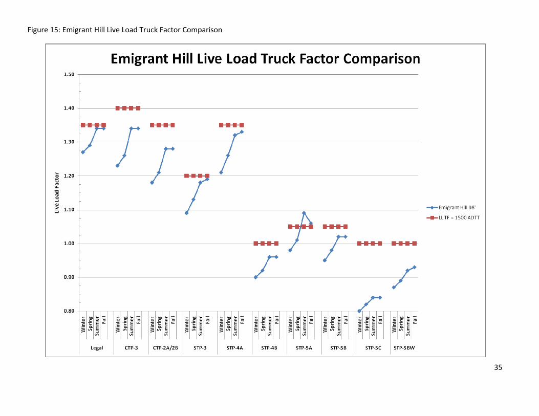
35

Figure 15: Emigrant Hill Live Load Truck Factor Comparison

36

Figure 16: Bend Live Load Truck Factor Comparison

37

Figure 17: Lowell Live Load Truck Factor Comparison

APPENDIX B Main Features of Selected Studies for Collecting and Using Traffic Data in Bridge Design The technical literature search resulted in the compilation of a reference list consisting of approximately 250 abstracts, research papers, journal articles, conference papers, and reports with applicability to the project research. Of the examined material, approximately 70 applicable documents were selected for further evaluation and possible summary preparation. A tabulated summary (given below) of approximately 40 documents was prepared from the reviewed material. Contained in each document summary is a brief study description, the study findings (if any), and recommendations for further research suggested by the authors (if any).

Reference

Study Description

Findings

Recommendations

Lui, Cornell and Imbsen Analysis of Bridge Truck Loads (1998)

Presents statistical analysis of truck loading variables including gross vehicle weight (GVW) data collected at several weigh-in-motion (WIM) sites on roadways of various functional classifications in Florida and Wisconsin. Discusses the application of WIM data and truck loading statistical analysis to site-specific load model development for bridge evaluation.

The upper tail of Florida GVW probability distribution data collected during this study is similar to the results of previous studies. The upper tail of collected Wisconsin GVW probability distribution data reveals two abnormalities in the data collected at several WIM sites: 1). Vehicles weighing in excess of 100 Kips, more than the 80 Kips legal limit, 2). Overloaded trucks weighing between 120 and 150 Kips.

Two distinct aspects of the site-specific load model for bridge rating are important: 1). Realistic assessment of the load level, 2). Uncertainty reduction associated with loads. To manage an aging infrastructure with limited available resources, site-specific load model development for bridge evaluation must critically assess the uncertainties of the random variables that make up the model.

Moses, Ghosn and Snyder Application of Load Spectra to Bridge Rating (1984)

Presents methods of acquiring and applying live load spectrum data at a bridge site for evaluation purposes. A reliability based model is described that can calibrate appropriate load factors, predict maximum expected truck loading, and incorporate the measured statistics of girder distribution and impact.

AASHTO girder distribution factors are generally conservative compared to measured values from WIM data when trucks are occupying two lanes. Design specification moments used in evaluation have a greater uncertainty than a measured load spectrum determined at the site.

Reduced load factors for permit loads may be warranted for permit loads if the loading is carefully controlled. Load and resistance factors in rating calculations need to differ from factors applied to design because of exposure period and available performance data.

B-1

Current User

Text Box

Appendix B: From NCHRP Report W135

Reference

Study Description

Findings

Recommendations

Miao and Chan Bridge Live Load Models from WIM Data (2002)

Hong Kong based study presents a new methodology for deriving highway bridge live load models for short span bridges using WIM data. Two methods are presented to obtain extreme daily bending moments using WIM data: 1). The lane loading model is derived based upon the equivalent base length concept, 2). The truck loading model is developed based upon a statistical approach. The developed lane and truck loadings are compared with other loading models adopted locally and overseas.

The developed Hong Kong Bridge Design Load (HKBDL) (per lane) was found to be best represented by the following: 1). For a span of 0 to 5 m – a single axle load of 15.0 t, 2). For a span of 5 to 23.5 m – a single axle load of 8.0 t plus a uniformly distributed load, 3). For a span greater than or equal to 23.5 m – a uniformly distributed load over 23.5 m. After studying five possible truck models, the developed HKBDL (standard truck) was determined to be best represented by a six axle vehicle with a total length of 14.0 m. Axle loads vary from 7.5 t to 11.0 t and axle spacings vary from 1.3 m to 4.0 m. The proposed design loadings for Hong Kong, developed assuming a probability of 0.98 of the heaviest vehicle in Hong Kong, induce forces that are less than the design loading standards of many other countries.

Additional work is necessary to consider shear effects and effects on continuous spans. Load factors need to be studied for various combinations of loadings.

Heywood and Nowak Bridge Live Load Models(1989)

Australian study presents the analysis of WIM data. The data is statistically analyzed and normalized by the National Association of Australian State Road Authorities (NAASRA) T44 design loading, and the results of analysis are compared to current Load and Resistance Factor Design (LRFD) loading limit states.

The ratio of ultimate limit state (ULS) to serviceability limit state (SLS) moments based on statistically analyzed WIM data is approximately constant for each distribution considered, however it varies from 1.1 to 1.4 for all of the distributions studied. The ratio of the largest ULS (recurrence interval distribution) to the smallest SLS (normal distribution) moments

Develop a new bridge design live load in place of the T44 loading in order to provide a more uniform prediction of the effects of traffic loads on a variety of bridge spans. Consider revising the recurrence interval for the serviceability limit state so that this condition does not control the bridge design.

B-2

Reference

Study Description

Findings

Recommendations

results in a value of 1.6. Similarly, the shear value varies from 1.4 to 1.5. Both the moment and shear values are less than the ultimate load factor of 2.0 that was proposed for the NAASRA Bridge Design Code.

Nowak and Hong Bridge Live-Load Models (1991)

Presents a statistical procedure for calculation of live-load moments and shears for highway girder bridges of various span lengths with one and two lane configurations and using truck survey data collected by the Ontario Ministry of Transportation. The maximum load effects for time periods from one day to 75 years are produced from extrapolations and simulations.

The maximum moment and shear for single lane bridges up to approximately 100 feet long result form the application of a single truck. The study shows that two trucks following each other produce the maximum moment and shear for longer single lane bridges. The simulation results indicate that that two side-by-side perfectly correlated truck or lane loads, depending upon bridge length, is the governing two lane bridge live load model.

None.

Nowak and Szerszen Bridge Load and Resistance Models (1998)

As a part of the development of rational codes (the AASHTO LRFD Bridge Design Specifications, Ontario Highway Bridge Design Code, and Eurocode) for the design of bridges and evaluation of existing structures, presents a procedure for statistically calculating the live-load moments and shears for highway girder bridges using truck survey data collected by the Ontario Ministry of Transportation. Resulting bias factors for live load from the analysis are presented with the corresponding changes to the design live loads for the national

The maximum moment and shear for single lane bridges up to approximately 30 to 40 m feet long result form the application of a single truck. The study shows that two fully correlated trucks following each other produce the maximum moment and shear for longer single lane bridges. The simulation results indicate that that two side-by-side perfectly correlated truck or lane loads, depending upon bridge length, is the governing two lane bridge live load model for interior girders. One truck may govern in some cases for exterior girders.

None.

B-3

Reference

Study Description

Findings

Recommendations

design codes.

The live load bias factors for moment and shear were found to be non-uniform for the span lengths investigated, necessitating a change in the live load model to produce a uniform factor. Current code girder distribution factors (GDF) were found to be inaccurate; long spans and large girder spacings result in conservative values, and short spans with small spacings result in non-conservative values.

Moses Calibration of Load Factors for Load and Resistance Factor Evaluation (1999)

Outlines the derivations of the live load factors in the proposed AASHTO Condition Evaluation Manual using truck weight spectra. The use of site specific traffic data is addressed.

Live load factor calibration, using similar data from the LRFD code development, was necessary to allow greater flexibility for evaluation as compared to design (varying site traffic and permits, and amount of site traffic data retrieved).

None.

Nowak and Grouni Calibration of the Ontario Highway Bridge Design Code 1991 Edition (1994)

Describes the calculation of load and resistance factors for the Ontario Highway Bridge Design Code (OHBDC) 1991 edition, including the development of load and resistance models utilizing available truck surveys from Ontario, the selection of the reliability analysis method, and the calculation of reliability indices for bridge design and evaluation.

An analysis of the reliability indices for girder bridge types designed per the OHBDC (1983) revealed that they are generally lower than the desired target for shorter spans. Therefore, the existing design truck tandem axle load was increased from 140 kN to 160 kN. For the evaluation of existing bridges, the time dependent load model results in shears and moments that are 3% to 5% lower than those used for design and lower reliability indices are generally used as compared to design.

The following are the results of this study: 1). For design, the live load was modified and the tandem axle load was increased to 160 kN. 2). Modified load and resistance factors should be used for the evaluation of existing bridges depending upon the frequency of inspection, if the components have single or multiple paths, and if the components are primary or secondary members.

Nowak Development of Bridge Load

Using truck surveys, weigh-in-motion measurements, and other

The values of live load moments and shear from truck survey data (number

Based upon the results of the two lane model simulation, the girder

B-4

Reference

Study Description

Findings

Recommendations

Model for LRFD Code (1993)

observations, this paper describes the development of the LRFD load model for static live load.

of axles and axle spacing, and axle loads and gross vehicle weight) are determined by extrapolation for a wide range of simple and continuous spans. Both one and two lane conditions are considered for time periods of 1 day to 75 years. For the one lane condition, the maximum lane moment or shear is caused by one truck, or two or more trucks following each other, depending upon span length. For the two lane condition, distribution of truck load to the girders is very important. Simulations reveal that for interior girders, the case of two fully correlated side-by-side trucks governs.

distribution factors specified by AASHTO (1992) are generally too conservative, particularly for larger girder spacing. The proposed LRFD live load is recommended as the following: 1). The superposition of an HS20 vehicle and a uniform load of 640 lb/ft. 2). For shorter spans a tandem is specified. 3). For negative moments, use two HS20 vehicles, however reduce the total effect by 10 percent.

Agarwal and Cheung Development of Loading-Truck Model and Live-Load Factor for the Canadian Standards Association CSA-S6 Code (1987)

Presents the methodology utilized to develop the CS-W loading design truck and uniform live load factor for the Canadian Standards Association CSA-S6 code. Truck survey data was collected in seven Canadian provinces and used in the development of the design load model and live load factor.

Using survey data from Newfoundland, Ontario, and Alberta, the study found that for spans up to 20m, the proposed CS-600 design truck requires a higher load factor, reflecting a deficiency in the live load model for short spans. The design load was revised to ensure a uniform live load factor. Using survey data from Nova Scotia, Quebec, Saskatchewan, and British Columbia, the study found that each province demonstrated live load factors of similar magnitude.

For all types of live-load effects and ranges of span lengths a uniform live-load factor of 1.60 should be adopted. The CS-600 loading should be adopted as the standard bridge design load for Canadian interprovincial truck routes. A load level different from the CS-600 loading may be adopted by provincial and local authorities.

Nowak and Nassif Live Load Models Based on WIM Data

Michigan bridge WIM study compares measurements taken on three instrumented US route and Interstate

Weigh station data greatly underestimates the gross vehicle weights of overloaded truck traffic in Michigan. Truck weigh

None.

B-5

Reference

Study Description

Findings

Recommendations

(1992) bridges to weigh station data.

station data is biased to less heavy vehicles due to trucker avoidance of the stationary scales. The study found that the gross weights collected at weigh stations were generally within the legal limits, however bridge WIM data shows that the structures are actually being significantly overloaded.

Heywood A Multiple Presence Load Model for Bridges (1992)

Australian study investigates the use of WIM data to simulate multi-lane traffic crossing short span multiple lane bridges. Two lane bridges with spans less than 30 m long are simulated in this study, as this model is representative of the majority of Australian bridges.

The multiple presence simulation models indicate that for low traffic volumes the serviceability recurrence interval is significantly less than the proposed AASHTO value considering that the ultimate limit state is far less sensitive to changing traffic volume.

None.

Jaeger and Bakht Multiple Presence Reduction Factors for Bridges (1987)

Paper reviews the multiple presence reduction factors specified in the AASHTO and Ontario codes and provides an alternate method for establishing these factors for short and medium span bridges in relation to traffic volume using truck survey data. Factors for design and evaluation are proposed.

The multiple presence reduction factors by the proposed method using traffic density and truck weight distribution data are not significantly different from those of the AASHTO and Ontario codes.

Traffic density should be one of the deciding factors in choosing a multiple presence reduction factor value for design and evaluation. The reduction factors used in evaluation should also consider the expected remaining bridge life, the number of loaded lanes, and the time interval for vehicle to cross the middle third of the bridge, using the procedure presented in the paper.

Fu and Hag-Elsafi New Safety-Based Checking Procedure for Overloads on Highway Bridges (1996)

Using WIM data from United States sites and NYSDOT overload permit data, this paper presents an evaluation method for nondivisible overload permit checking using the LRFD concept of uniform bridge safety.

The paper proposes live load factors to be used in the checking procedure for annual and trip permits for overloaded trucks.

Incorporation of this bridge evaluation method for overweight trucks into code may be considered.

Fujino and Ito Utilizing data from The study shows that the A revised design load is

B-6

Reference

Study Description

Findings

Recommendations

Probabilistic Analysis of Traffic Live Loading on Highway Bridges (1979)

surveys of traffic loads carried out on several Japanese highways, this paper summarizes the statistical analysis using computer simulation for the appraisal of the current design load and the development of a new design load.

current design load provides a safety reserve that is not constant for bridges of different span lengths, with a greater safety level provided for longer spans.

proposed, however the authors suggest analysis of continuous span bridges and further investigation of traffic flow on bridges.

Ghosn and Moses Reliability Calibration of Bridge Design Code (1986)

This study is the reliability calibration of the AASHTO bridge design code. The study incorporates two important concepts in bridge design load modeling: 1). The use of WIM to provide data on bridge loading and response for short and medium span bridges. 2). The use of reliability-based design to provide uniform reliability through a combined selection of nominal design loads and corresponding safety margins.

The reliability-based calibration of the AASHTO bridge design code revealed the following: 1). The AASHTO code provides high levels of reliability, but does not provide uniform reliability levels for all span lengths. 2). New safety factors and design loads are proposed to achieve uniform reliabilities or safety indices. 3). The target safety index was derived from average AASHTO performance. 4). The derived partial safety factors achieved more uniform safety indices. 5). Different live load factors are desirable for different loading intensities. 6). This approach to load modeling can be applied to bridge evaluation.

None.

Ghosn and Frangopol Site-Specific Live Load Models for Bridge Evaluation (1996)

Study focuses on the use of WIM to define site-specific bridge loads, and the differences in safety that result from applying site-specific values to evaluation rather than the national average (design loads).

For the bridge evaluation example presented, a safety index of 4.07 resulted from the use of the method presented in the Nowak (1993) model for design. Repeated with site-specific WIM data from two independent sites, the example resulted in safety indices of 3.69 and 3.03, displaying that the use of site-specific

The use of average live load data in the assessment of existing bridge reliability may not be representative of actual site conditions and actual site loading from WIM data should be utilized.

B-7

Reference

Study Description

Findings

Recommendations

load data provides results that are different than those obtained from typical data.

Laman and Nowak Site-Specific Truck Loads on Bridges and Roads (1997)

This study uses bridge WIM data to determine and compare site-specific bridge live loads at several locations on Interstate highways, state highways, US highways, and surface streets in Michigan. Weigh station data and truck citation data is utilized to verify the recorded truck loads by WIM.

The study shows that truck loads are strongly site specific and depends on factors such as traffic volume, local industry, and law enforcement effort. A negative correlation was found between law enforcement effort and the occurrence of overloaded trucks as overloaded trucks were found on roadways not controlled by truck weigh stations.

Additional truck data is needed to determine the site-specific load spectra for bridges. Rather than utilizing truck weigh station data, which is biased due to avoidance, unbiased WIM data is needed to determine accurate statistics for site-specific bridge live load models.

Nowak and Ferrand Truck Load Models for Bridges (2004)

Michigan bridge WIM study reviews some of the practical procedures used for field measurement of truck weights and uses this data to simulate site-specific truck loads.

The results of the WIM measurements show that truck traffic is strongly site specific and varies within a geographic area based on the number of trucks, gross vehicle weight, and axle weight. The study found that the shapes of the moment and shear distributions are almost identical, simplifying the bridge evaluation procedure since the same live load factors can be used for both moment and shear. Using the collected WIM data, maximum lane moments and shears were computed and compared to the AASHTO LRFD 1998 moments and shears. The maximum lane moments and shears due to the measured trucks vary between 0.6 and 2.0 times the AASHTO values.

None.

Frangopol, Goble and Tan Truck Loading Data for a Probabilistic

Study consists of a major bridge testing and analysis program for the FHWA. Thirty-five bridges in thirteen states

The study classified approximately 160,000 truck occurrences. Of these occurrences, approximately 6,881 fell

The data will be employed in the development of improved live load models for bridge design and

B-8

Reference

Study Description

Findings

Recommendations

Bridge Live Load Model (1992)

were tested using WIM. into the multiple presence category, defined as a front axle-to-front axle spacing between vehicles of less than 120 feet. Side-by-side multiple presence was separated from same-line multiple presence. 5,516 side-by-side and 1,365 same-line multiple presence situations were recorded.

evaluation.

Fu and Hag-Elsafi Vehicular Overloads: Load Model, Bridge Safety, and Permit Checking (2000)

This study develops a live load model for truck traffic including overloads. The model is used to assess bridge safety subject to overloads and is designed to incorporate site-specific WIM data.

The paper proposes live load factors to be used in the checking procedure for annual and trip permits for overloaded trucks, consistent with the average bridge safety by the AASHTO code.

Consideration may be given to incorporating this bridge evaluation method for overloaded trucks into code.

Ghosn, Moses and Gabriel Truck Data for Bridge Load Modeling (1990)

Utilizing WIM data collected at several steel multi-girder Interstate bridges in Ohio, this study applies a simulation program that estimates the probabilistic distribution of maximum moment response of bridges. The study uses the model to develop a reliability-based truck weight formula that regulates the weight of trucks on US bridges. The developed truck weight formula is applicable to simply supported steel bridges designed for AASHTO’s WSD HS20 loading and will have a .25 safety index for a 50 year life.

In the calculation of the truck weight formula, H, the random variable that gives the overload factor due to the presence of closely spaced vehicles, was found to be sensitive to only very large changes in truck volumes.

None.

Nyman Calibration of Bridge Fatigue Design Model (1985)

This study consists of a structural reliability evaluation of the current AASHTO fatigue specification for steel bridges using field data obtained from a bridge-mounted WIM system. A fatigue life failure model

The study has determined the following: 1). The proposed fatigue vehicle model is more representative of the current truck traffic at sites examined in the US. 2). The current AASHTO code appears to lead to

The proposed revisions to the current specification include: 1). Replacement of the current AASHTO fatigue design load model with Pavia’s vehicle. 2). Modification of the allowable stress ranges to

B-9

Reference

Study Description

Findings

Recommendations

is formulated in terms of a fatigue failure function.

safety indices that vary with the different stress categories. 3). Truck traffic including weight and volume vary too much from site to site to be covered by only two categories as currently done.

give a more uniform safety index for all stress categories. 3). Specification of different load factors for a range of volumes and loadometer values. 4). Refinement of the failure function variables to provide a more accurate safety index. The relationship between truck headway and volume also needs to be determined.

Caprani, Grave, O’Brien and O’Connor Critical Loading Events for the Assessment of Medium Span Bridges (2002)

Using WIM data from a French site, this study is the Monte-Carlo simulation of free-flowing traffic across bridges to determine the critical loading events and extreme load effects (bending moment and shear force).

The study shows that the two-truck event is the most important free-flowing event for short to medium span bridges with two opposing lanes of traffic. For longer spans, events involving three or more trucks can be significant.

Both two and three truck events should be modeled in the assessment of site-specific bridge loading for structure lengths up to 50 m and in free flowing situations.

Laman and Nowak Fatigue-Load Models for Girder Bridges (1996)

This paper focuses on the development of a new fatigue-load model for steel girder bridges using WIM data from five bridges. The data from the five structures consists of site-specific truck parameters and component-specific stress spectra.

The study findings indicate that the magnitude and frequency of truck loading are site-specific and component-specific. The results also reveal a significant variation in stress spectrum between girders. Generally, the girder that is located nearest to the left wheel track of vehicles traveling in the right lane experiences the highest stresses in the stress spectra and decreases as a function of the distance from this location. It was found that a vehicle that dominates the distribution of vehicle types does not necessarily dominate the fatigue damage of the particular component. Rather, a vehicle that dominates the distribution of the lane

A single truck model for fatigue loading is not recommended as the most accurate approach as a result of the site-specific nature of the distribution of vehicle types by axle. The paper recommends the use of an equivalent three axle fatigue truck with varying axle weight and spacings for sites with traffic consisting of two to nine axle trucks. Similarly, for sites with ten and eleven axle trucks, a four axle truck is recommended as an equivalent fatigue vehicle.

B-10

Reference

Study Description

Findings

Recommendations

moments will likely dominate the fatigue analysis.

Au, Lam, Agarwal and Tharmabala Bridge Evaluation by Mean Load Method per the Canadian Highway Bridge Design Code (2005)

This paper summarizes bridge evaluation by the Canadian Highway Bridge Design code (CHBDC) mean load method. The mean load method does not require the use of load or resistance factors. Instead, the uncertainties associated with the loads and resistances are considered by using default statistical parameters. The code also allows the use of parameters that are derived from collected site-specific WIM data. The paper compares the results of a steel box girder bridge evaluation using the mean load method default parameters, WIM derived parameters, and the LRFD method.

A comparison of the evaluation results shows that the LRFD method and the mean load method using the default statistical parameters provide similar results, with the mean load method offering a slightly higher live load capacity factor. The mean load method using live load statistics based on WIM data, provides the highest load carrying capacity. This is a result of the conservative statistical parameters provided in the CHBDC.

Mean load method evaluation results using WIM data may not be conclusive if the bridge’s most critical traffic loading periods are missed during field data collection. The season and measurement periods require thoughtful selection to capture the most critical live loading on the bridge.

van de Lindt, Fu, Zhou and Pablo Locality of Truck Loads and Adequacy of Bridge Design Load (2005)

This paper investigates the differences in live loading conditions between the national average as utilized in the AASHTO LRFD code and twenty site-specific Detroit, Michigan girder bridge locations. Resulting reliability indices are compared. WIM data is used to characterize the truck load effect in the bridges’ primary members for moment and shear at critical cross sections.

This study established the following: 1). In general, the local truck loading may vary significantly from the state or national average, resulting in inconsistent risk levels for highway bridges. 2). Based upon the study findings of the twenty subject bridges, the current Michigan HS25 design load does not consistently achieve a reliability index of 3.5 for the design-minimum strength of bridges in the Detroit area.

This WIM data used in this study did not include headroom information. Further study incorporating WIM data with headroom information should be performed to advance the study topic. Site-specific live load analyses are necessary, particularly for trunkline roadways with high ADTTs, in order to achieve a more uniform reliability index. Consideration should be given to performing a feasibility study at the national level.

Cohen, Fu, Dekelbab and Moses

Using WIM and truck survey data, this study presents a qualitative

This study has established the following: 1). The modeling is based

None.

B-11

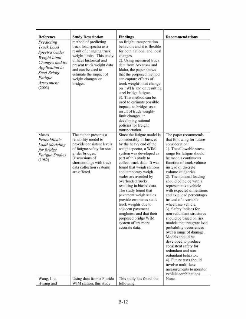
Reference

Study Description

Findings

Recommendations

Predicting Truck Load Spectra Under Weight Limit Changes and its Application to Steel Bridge Fatigue Assessment (2003)

method of predicting truck load spectra as a result of changing truck weight limits. This study utilizes historical and present truck weight data and can be used to estimate the impact of weight changes on bridges.

on freight transportation behavior, and it is flexible for both national and local changes. 2). Using measured truck data from Arkansas and Idaho, the paper shows that the proposed method can capture effects of truck weight-limit change on TWHs and on resulting steel bridge fatigue. 3). This method can be used to estimate possible impacts to bridges as a result of truck weight-limit changes, in developing rational policies for freight transportation.

Moses Probabilistic Load Modeling for Bridge Fatigue Studies (1982)

The author presents a reliability model to provide consistent levels of fatigue safety for steel girder bridges. Discussions of shortcomings with truck data collection systems are offered.

Since the fatigue model is considerably influenced by the heavy end of the weight spectra, a WIM system was developed as part of this study to collect truck data. It was found that weigh stations and temporary weigh scales are avoided by overloaded trucks, resulting in biased data. The study found that pavement weigh scales provide erroneous static truck weights due to adjacent pavement roughness and that their proposed bridge WIM system offers more accurate data.

The paper recommends that following for future consideration: 1). The allowable stress range for fatigue should be made a continuous function of truck volume instead of discrete volume categories. 2). The nominal loading should coincide with a representative vehicle with expected dimensions and axle load percentages instead of a variable wheelbase vehicle. 3). Safety indices for non-redundant structures should be based on risk models that integrate load probability occurrences over a range of damage. Models should be developed to produce consistent safety for redundant and non-redundant behavior. 4). Future tests should involve multi-lane measurements to monitor vehicle combinations.

Wang, Liu, Hwang and

Using data from a Florida WIM station, this study

This study has found the following:

None.

B-12

Reference

Study Description

Findings

Recommendations

Shahawy Truck Loading and Fatigue Damage Analysis for Girder Bridges Based on Weigh-in-Motion Data (2005)

synthesizes the truck traffic data and establishes the live-load spectra, and performs a fatigue damage analysis for six typical steel multi-girder bridge models that were generated for this project.

1). Flexural stress and shear vary with bridge span length. 2). Truck loading on the bridges does not necessarily increase with GVW, but rather with axle weight. Tandem axles significantly exceed the loading of an HS20-44 vehicle. 3). The average impact factors are generally less than the values specified in AASHTO (1996). 4). The AASHTO fatigue truck and the actual truck-traffic flow based on with measurements have close effects.

Grundy and Boully Fatigue Design in the New Australian Bridge Design Code (2004)

This paper presents an overview of the work performed in developing the fatigue provisions for the new Australian Bridge Design Code AS5100. Calibration of the fatigue loading model against Culway WIM data is described. The projected growth in traffic volume and magnitude of vehicle and axle mass is incorporated in the fatigue loading model.

The following was noted: 1). Span has a great effect on the fatigue damage per truck. For short steel bridges, fatigue can become the governing limit state for structures on heavily traveled roadways. For longer spans, fatigue is not as great an issue due to the effect of dead load. 2). Multiple presence of trucks in the same or adjacent lanes occurs infrequently per the WIM data.

None.

Jamera et al FHWA Study Tour for European Traffic-Monitoring Programs and Technologies (1997)

This FHWA-sponsored study is a scanning tour of the Netherlands, Switzerland, Germany, France, and the United Kingdom. The tour was conducted in order to learn how European countries perform traffic monitoring and if and how these concepts can be applied in the United States. Several areas of specific interest regarding WIM system and data collection were reviewed

The study found the following: 1). Fewer and less detailed data are collected on trucks than in the US. 2). Standardization of data collection equipment is common. The Europeans are working to coordinate WIM research and development to produce better, more reliable WIM equipment (DIVINE, COST 323, and WAVE projects). 3). WIM systems require

The study recommends that there are two areas in which US transportation experts should pay attention to European WIM systems and activities: 1). The Europeans employ limited classification schemes, allowing the use of less sophisticated and less costly collection equipment. An analysis of cost savings versus loss of detailed

B-13

Reference

Study Description

Findings

Recommendations

and summarized. calibration at least twice a year. 4). Only France and the United Kingdom have extensive WIM system installations.

information requires analysis. 2). The COST and WAVE WIM tests should be monitored by US researchers to eliminate duplicate efforts in this county.

O’Brien and Caprani Headway Modelling for Traffic Load Assessment of Short to Medium Span Bridges (2005)

The assumed headways of successive trucks on bridges have a great impact on the critical loading events from which the characteristic effects are derived. This paper presents a new approach that uses measured headway statistical distributions generated from French WIM data.

The following has been established from this study: 1). Headways of less than 1.5 sec. were found to be insensitive to traffic flow and are influenced by driver behavior. Headways between 1.5 sec. And 4.0 sec. were found to be considerably influenced by traffic flow. 2). Assumptions related to headways and gaps have a great impact on load effects and characteristic values.

The authors recommend a statistical (HeDS) approach for site-specific assessment of bridge loading.

van de Lindt, Fu, Pablo and Zhou Investigation of the Adequacy of Current Design Loads in the State of Michigan (2002)

This report presents the process and results of a research effort to examine the adequacy of current vehicle loads used to design bridges in the State of Michigan. The target reliability index used in the AASHTO LRFD code was utilized in the study as the criterion for evaluating the adequacy. Reliability indices were calculated for twenty different bridges selected from the Michigan inventory of new bridges. Existing WIM data was processed to statistically characterize the truck load effect.

The following conclusions were made by the report: 1). The reliability indices were found to vary among bridge types. 2). The 50th and 90th percentile of traffic volume do not noticeably influence the reliability indices. 3). The current design load, HS25, could be modified to achieve, on average, a reliability index of 3.5, which was used as a target index for the AASHTO LRFD code. 4). The deck design load of HS20 is adequate for reinforced concrete decks.

The authors recommend that a new design load level be considered for bridge beam design in the Detroit Metro Region.

Nichols and Bullock Quality Control Procedures for Weigh-in-Motion Data

This study consists of the development of a quality control program for the Indiana Department of Transportation to improve the accuracy of

The study found the following: 1). The WIM applications at static weigh stations were effective for identifying safety

The study recommended the following: 1). The drive tandem axle spacing metric should be applied to all WIM systems to monitor the

B-14

Reference

Study Description

Findings

Recommendations

(2004) the data produced from their WIM sites. The quality control program is based on the Six Sigma quality control program DMAIC performance improvement model and provides a mechanism for assessing the accuracy of vehicle classification, weight, speed, and axle spacing data and monitoring it over time.

violations, but ineffective for identifying overweight vehicles. Virtual weigh stations in Indiana were found to be approximately 55 times more effective than the static weigh stations for overweight truck identification. 2). Robust metrics for speed and axle spacing accuracy, weight accuracy, and sensor error rates are necessary in a quality control program that can be continuously monitored using statistical process control procedures. 3). Data mining of these metrics revealed variations in the data caused by incorrect calibration, sensor failure, temperature, and precipitation.

speed calibration and prioritize maintenance on a lane basis. 2). The bending plate and single load cell WIM systems should be configured to log the left and right wheel data to compute the left-right residual metric. Use the left-right residual for detecting weight calibration drift and to prioritize maintenance on a lane basis. 3). The error proportion metric should be applied to all WIM systems to identify lanes that experience high error rates to prioritize maintenance on a lane basis. 4). The WIM data should be continuously monitored for errors and drifts to establish and maintain accurate data. 5). The WIM system algorithms should consider variations in the climate to account for temperature and precipitation or flag data that is collected during days of climatic anomalies when the accuracy is questionable. 6). To apply the recommended quality control procedures, the WIM data must be uploaded to a relational database that supports free-form queries. Analysis cubes are recommended for data mining. 7). A test bed should be constructed of various types of WIM sensor for long-term evaluation of performance, accuracy, and maintenance costs for

B-15

Reference

Study Description

Findings

Recommendations each type. Installation of equipment to collect continuous climate data would allow further exploration of the climatic impacts on the WIM sensors.

Hwang and Koh Simulation of Bridge Live Load Effects (2000)

The current design load in Korea, which is not based on any research or actual data, was adopted in 1978. This paper presents the research for the new live load model for the reliability-based design code that is based on collected bridge WIM data and video recording. The new model is compared to the design live load model from several countries.

The study has determined the following: 1). The new live load model should consist of a combination of truck load and distributed load with a varying magnitude based on span length. 2). Weight distributions differ for each WIM site and direction, highlighting the importance of accurate data for the live load model. 3). The maximum moment ratio is variable based on span length. A single truck controls for shorter span lengths and two fully correlated trucks govern for longer spans.

The paper suggests that additional data should be collected to better represent truck load effects.

O’Connor and O’Brien Traffic Load Modelling and Factors Influencing the Accuracy of Predicted Extremes (2005)

This paper describes traffic simulation (direct and Monte Carlo method) using European WIM statistics for the assessment of existing bridges. The implications of the accuracy of the recorded data and the duration of recording and of the sensitivity of the extreme to the method of prediction are investigated. Traffic evolution with time is also explored.

The paper offers the following findings: 1). The accuracy of the extreme load effects by Monte Carlo simulation increases with increasing span length in inverse proportion to the variance in the extreme. 2). A comparison of extrapolation techniques shows the importance of appropriate selection of an extreme value distribution. 3). The accuracy of WIM data is more critical for shorter span lengths. The effects of increasing inaccuracy were seen to attenuate with span. 4). The time-dependent and seasonal analyses do not provide any clear

None.

B-16

Reference

Study Description

Findings

Recommendations

proof of a seasonal trend. 5). When considering future growth, it is found that the factor that could have major influence on predicted extremes in the future is a change allowable gross vehicle weight. 6). The sensitivity of characteristic extremes to the duration of recording and the amount of available data is a function of the effect and span under consideration.

Lu, Harvey, Le, Lea, Quinley, Redo and Avis Truck Traffic Analysis Using Weigh-In-Motion (WIM) Data in California (2002)

This report is based on truck traffic data collected from all of the WIM stations on the California State highway network. Two objectives of the study were to determine truck traffic volume and load growth trends using regression methods and to check the possibility of extrapolating available truck traffic data to sites where WIM stations are not installed.

The report concluded the following: 1). Axle load spectra are heavier at night than during the daytime, possibly due to more efficient operation without car traffic or avoidance due to closure of more weigh stations. 2). Axle load spectra shows little seasonal variation. 3). Axle load spectra are much higher at rural WIM stations compared to urban stations, likely due to the presence of more long-haul trucking at rural WIM stations, and more short-haul, less-than-full-load trucking in urban areas. 4). The proportion of larger truck types, which would more typically be used for long-haul trucking, increases at night. 5). The analysis of six representative WIM sites shows that GVW generally did not grow across the six sites. Although the number of trucks using the highways increased, the trucks were

The following recommendations were made: 1). Further research should be conducted to improve methods of estimation for locations that are not equipped with WIM systems. 2) Several recommendations were made regarding improvement to the capability of the WIM data collection system including regular quality assurance checks and maintenance at all WIM stations.

B-17

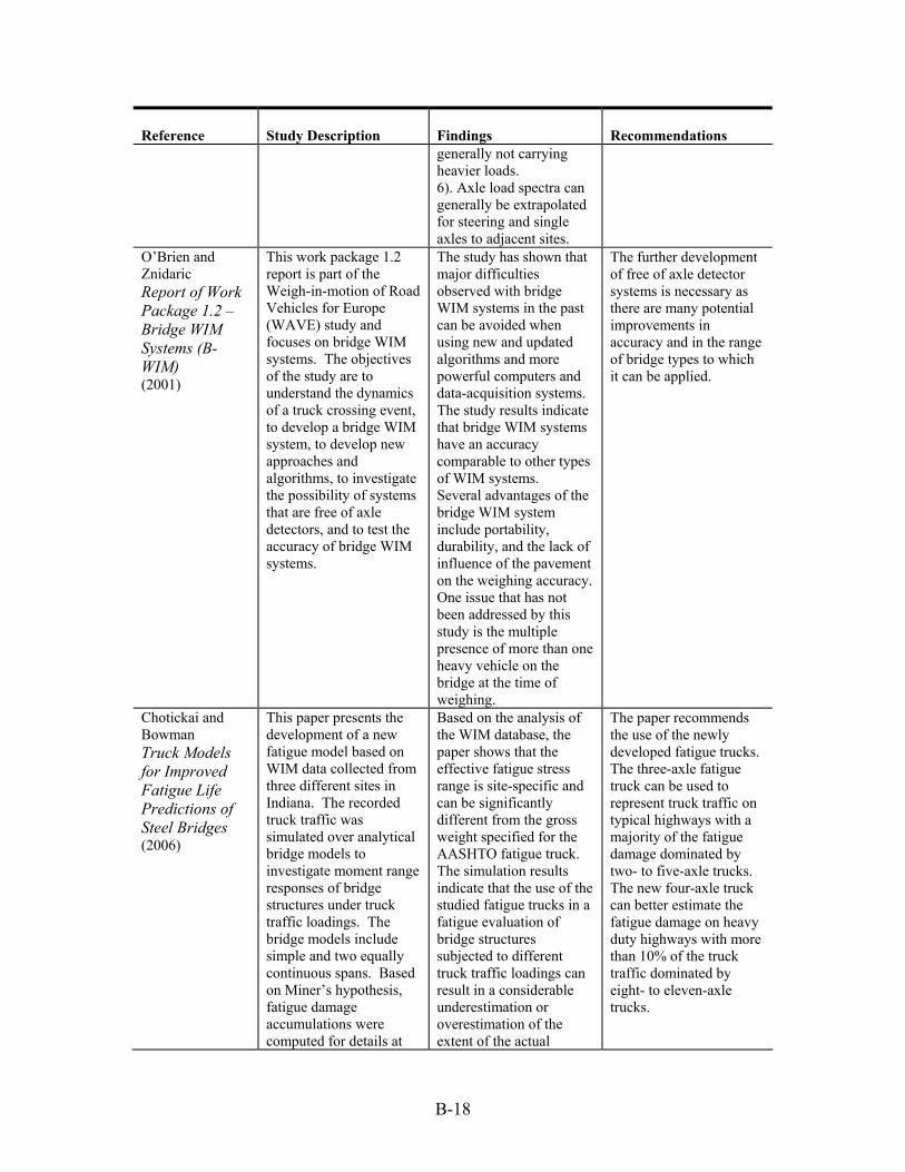
Reference

Study Description

Findings

Recommendations

generally not carrying heavier loads. 6). Axle load spectra can generally be extrapolated for steering and single axles to adjacent sites.

O’Brien and Znidaric Report of Work Package 1.2 – Bridge WIM Systems (B-WIM) (2001)

This work package 1.2 report is part of the Weigh-in-motion of Road Vehicles for Europe (WAVE) study and focuses on bridge WIM systems. The objectives of the study are to understand the dynamics of a truck crossing event, to develop a bridge WIM system, to develop new approaches and algorithms, to investigate the possibility of systems that are free of axle detectors, and to test the accuracy of bridge WIM systems.

The study has shown that major difficulties observed with bridge WIM systems in the past can be avoided when using new and updated algorithms and more powerful computers and data-acquisition systems. The study results indicate that bridge WIM systems have an accuracy comparable to other types of WIM systems. Several advantages of the bridge WIM system include portability, durability, and the lack of influence of the pavement on the weighing accuracy. One issue that has not been addressed by this study is the multiple presence of more than one heavy vehicle on the bridge at the time of weighing.

The further development of free of axle detector systems is necessary as there are many potential improvements in accuracy and in the range of bridge types to which it can be applied.

Chotickai and Bowman Truck Models for Improved Fatigue Life Predictions of Steel Bridges (2006)

This paper presents the development of a new fatigue model based on WIM data collected from three different sites in Indiana. The recorded truck traffic was simulated over analytical bridge models to investigate moment range responses of bridge structures under truck traffic loadings. The bridge models include simple and two equally continuous spans. Based on Miner’s hypothesis, fatigue damage accumulations were computed for details at

Based on the analysis of the WIM database, the paper shows that the effective fatigue stress range is site-specific and can be significantly different from the gross weight specified for the AASHTO fatigue truck. The simulation results indicate that the use of the studied fatigue trucks in a fatigue evaluation of bridge structures subjected to different truck traffic loadings can result in a considerable underestimation or overestimation of the extent of the actual

The paper recommends the use of the newly developed fatigue trucks. The three-axle fatigue truck can be used to represent truck traffic on typical highways with a majority of the fatigue damage dominated by two- to five-axle trucks. The new four-axle truck can better estimate the fatigue damage on heavy duty highways with more than 10% of the truck traffic dominated by eight- to eleven-axle trucks.

B-18

B-19

Reference

Study Description

Findings

Recommendations

various locations on the bridge models and compared with the damage predicted for the AASHTO fatigue truck, a modified AASHTO fatigue truck with an equivalent gross weight, and other fatigue truck models.

fatigue damage when compared to the damage predicted using the WIM database.

Tallin and Petreshock Modeling Fatigue Loads for Steel Bridges (1990)

Using WIM data from seven states, histograms of truck GVW are analyzed. These histograms are modeled by two bimodal distributions. Fatigue lifetimes for AASHTO categories A, B, C, and E details are calculated from these distribution of GVW models by approximating the Miner’s stress as a linear function of the mth root of the mth expected moment of the GVW. The lifetimes based on the two models are compared with each other and with the results obtained by assuming a single lognormal distribution.

The study results show that the fatigue lifetimes for AASHTO categories A, B, C, and E details estimated using the bimodal distributions differ little from each other but are significantly shorter than the lifetimes estimated from the single lognormal distribution. It was also noted that there are large differences between the estimated lifetimes of different AASHTO fatigue categories.

None.

LRFD-LRFR Preliminary Investigation 12-16-09 - … · in the AASHTO Manual for Bridge Evaluation...

Documents

Transcript of LRFD-LRFR Preliminary Investigation 12-16-09 - … · in the AASHTO Manual for Bridge Evaluation...