Low Stream Flows: Making Decisions in an Uncertain...

Low Stream Flows: Making Decisions in an

Uncertain Climate

by Dorian Turner

B.Sc. (Biology), University of Calgary, 2005

Research Project Submitted in Partial Fulfillment

of the Requirements for the Degree of

Master of Resource Management

in the

School of Resource and Environmental Management

Faculty of the Environment

Report No. 528

© Dorian Turner 2012

SIMON FRASER UNIVERSITY Spring 2012

All rights reserved. However, in accordance with the Copyright Act of Canada, this work may

be reproduced, without authorization, under the conditions for “Fair Dealing.” Therefore, limited reproduction of this work for the

purposes of private study, research, criticism, review and news reporting is likely to be in accordance with the law, particularly if cited appropriately.

ii

Approval

Name: Dorian Turner Degree: Master of Resource Management Report No. 528 Title of Thesis: Low Stream Flows: Making Decisions in an Uncertain

Climate

Examining Committee:

Randall Peterman Senior Supervisor Professor School of Resource and Environmental Management Simon Fraser University

Mike Bradford Supervisory committee member Adjunct Professor School of Resource and Environmental Management Simon Fraser University

Date Defended/Approved:

Jeremy Venditti Supervisory committee member Assistant Professor Department of Geography Simon Fraser University

iii

Partial Copyright Licence

iv

Abstract

Water resource managers must make decisions regarding minimum instream

flow requirements for rivers, despite many uncertainties. Two important uncertainties

concern (1) estimates of usable fish habitat at different discharges, and (2) effects of

climate change on future stream discharge. I examined the implications of these two

uncertainties for the North Alouette River, British Columbia (BC). Using the British

Columbia Instream Flow Methodology, which is an assessment method for water

diversions needed by small-scale hydroelectric projects, I found that uncertainty in

habitat preferences of rainbow trout (Oncorhynchus mykiss) fry generally dominated

uncertainty in the results of the BCIFM when numerous transects were used. In contrast,

for fewer than 15 transects, variation in physical habitat among sampled transects was

the most important source of uncertainty. In addition, the increasing frequency of climate

driven low-flow events suggests that operations of small-scale hydroelectric projects in

BC may become more restricted in the future.

Keywords: Instream flow needs; low-flow period; fish habitat; run-of-river hydroelectric generation; climate change; small streams;

v

Dedication

To everyone who helped to motivate and support me

through the past two and a half years - you know who you are.

vi

Acknowledgements

First and foremost, I would like to thank my supervisory committee, Randall

Peterman, Mike Bradford, and Jeremy Venditti, who have trusted and supported me with

my research interests. I would also like to thank Adam Lewis (Ecofish Research Ltd.),

Scott Babakaiff (MOE), Jordan Rosenfeld (UBC/MOE), Ron Ptolemy (MOE), James

Bruce (BC Hydro), and Don Reid (BC Hydro) for your much needed professional advice.

Thanks to Ionut Aron and the staff at the UBC Malcom Knapp Research Forest for

allowing me access to the beautiful North Alouette River. Thanks to the Fisheries

Science and Management Research Group at REM for your ongoing support. Last but

not least, thanks to those who spent tiring days splashing around in the North Alouette

River with me: Herb Herunter, Louise de Mestral Bezanson, Cameron Noble, and

Rachel Romero.

Funding for this project was provided by DFO (Fisheries and Oceans Canada)

through CRMI (Cooperative Resource Management Institute), CCIRC (Climate Change

Impact Research Consortium), and the NSERC HydroNet Network.

vii

Table of Contents

Approval............................................................................................................................. ii Partial Copyright Licence .................................................................................................. iii Abstract............................................................................................................................. iv Dedication ..........................................................................................................................v Acknowledgements...........................................................................................................vi Table of Contents............................................................................................................. vii List of Tables..................................................................................................................... ix List of Figures ...................................................................................................................xi List of Acronyms ............................................................................................................. xiii

Chapter 1. General Introduction ............................................................................... 1 References........................................................................................................................ 4

Chapter 2. Evaluating Uncertainty in the British Columbia Instream Flow Methodology in a High-Gradient Mountain Stream.............................. 6

Introduction ....................................................................................................................... 6 Methods ............................................................................................................................ 9

Field Site .................................................................................................................. 9 Physical Habitat Data............................................................................................. 10 Habitat Preference Data ........................................................................................ 10 Habitat-Flow Relation............................................................................................. 11 HSI Uncertainty...................................................................................................... 12 Physical Habitat Uncertainty .................................................................................. 12 Combined Uncertainty ........................................................................................... 13 Habitat Loss ........................................................................................................... 14

Results ............................................................................................................................ 14 HSI Uncertainty...................................................................................................... 14 Physical Habitat Uncertainty .................................................................................. 14 Combined uncertainty ............................................................................................ 15 Habitat Loss ........................................................................................................... 15

Discussion....................................................................................................................... 16 Evaluating Uncertainty ........................................................................................... 16 Habitat Loss ........................................................................................................... 19

Conclusion ...................................................................................................................... 20 Tables ............................................................................................................................. 22 Figures ............................................................................................................................ 25 References...................................................................................................................... 35

Chapter 3. Modeling the Relationship Between Climate and the Natural Low-Flow Period in the North Aloutte River, BC................................ 39

Introduction ..................................................................................................................... 39 Methods .......................................................................................................................... 41

Study Stream ......................................................................................................... 41 Streamflow data ..................................................................................................... 42 Climate data........................................................................................................... 43

viii

Linear regression models and model selection...................................................... 43 Model averaging .................................................................................................... 44 Climate projections ................................................................................................ 45 Low-flow projections .............................................................................................. 46

Results ............................................................................................................................ 46 Historical trends in the low-flow period .................................................................. 46 Historical trends in climate ..................................................................................... 47 Multi-model averaged linear regression................................................................. 47 Climate projections ................................................................................................ 47 Low-flow projections .............................................................................................. 48

Discussion....................................................................................................................... 48 Historical trends in climate ..................................................................................... 48 Historical trends in the low-flow period .................................................................. 50 Effects of climate variables on the low-flow period ................................................ 50 Climate projections ................................................................................................ 51 Low-flow projections .............................................................................................. 53

Conclusion ...................................................................................................................... 54 Tables ............................................................................................................................. 56 Figures ............................................................................................................................ 64 References...................................................................................................................... 68

Chapter 4. General Conclusion .............................................................................. 71

ix

List of Tables

Table 1.1. Estimated maximum weighted usable width (WUW) and optimal discharge from the habitat-flow relation produced by each of the five habitat preference curves (A-E) and the combined HSI (F). Habitat-flow relations shown in Figure 1.5. Letter correspond to the habitat preference curves from Figure 1.2. ............................................................... 22

Table 1.2. Median, empirical 95% confidence interval (CI), and coefficient of variation (CV) of the estimated maximum weighted usable width (WUW) and optimal discharge from the habitat-flow relations produced when incorporating (1) uncertainty from the combined habitat suitability indices (cHSI) with the transects fixed, (2) variability among transects but using a constant cHSI, and (3) both sources of uncertainty. Habitat-flow relations shown in Figure 1.7. ............................... 23

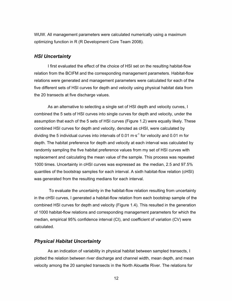
Table 1.3. Median, empirical 95% confidence interval (CI), and coefficient of variation (CV) of the estimated maximum weighted usable width (WUW) and optimal discharge from the habitat-flow relations produced when bootstrapping the variability among transects for a range of numbers of transects sampled. Habitat-flow relations were generated with constant combined habitat suitability indices (cHSI) curves. .......................................................................................................... 24

Table 2.1. Candidate models and corresponding AICc, ∆AICc, and AICc weights (wi) to explain number of days that discharge in the North Alouette River fell below 0.45, 0.35, and 0.25 m3/s from 1970-2010. Models are ordered by ∆AICc. Parameter symbols are: P (summer average daily precipitation), T (summer average daily temperature), and S (spring snowpack level). Interactions are represented by *. ......................... 56

Table 2.2. Top model set R (∆AICc <4), corresponding ∆AICc values, and re-scaled AICc weights (wi) to explain the number of days that discharge in the North Alouette River fell below 0.45, 0.35, and 0.25 m3s-1 from 1970-2010. Parameter symbols are: P (summer average daily precipitation), T (summer average daily temperature), and S (spring snowpack level). Interactions are represented by *. ..................................... 58

Table 2.3. The average number of days the discharge in the North Alouette River fell below 0.45, 0.35, and 0.25 m3s-1 in 1970 and 2010, with the average annual rate of change from the time-trend regression, including 95% confidence intervals and a p-value from the linear regression analysis. ...................................................................................... 59

x

Table 2.4. The average summer daily average temperature, summer daily average precipitation, and spring (April 1st) snowpack levels in 1970 and 2010, with the average annual rate of change for each climate variable from the time-trend regression, including 95% confidence intervals and a p-value from the linear regression analysis. ......................... 60

Table 2.5. Model-averaged parameter coefficient estimates in standard deviation units (SDU) to explain number of days that discharge fell below 0.45, 0.35, and 0.25 m3s-1 in North Alouette River, reported with the R2

value, unconditional standard errors (SE), 95% confidence intervals (CI) and Relative Variable Importance (RVI). Parameter symbols are: P (summer average daily precipitation), T (summer average daily temperature), and S (spring snowpack level). Interactions are represented by *............................................................................................ 61

Table 2.6. Observed (in 2010) and projected (in 2050) average summer mean daily temperature, summer mean daily precipitation, and spring (April 1st) snowpack levels with 95% confidence intervals and the probability that the variable will increase relative to 2010 levels, based on historical rates of change (Table 2.4)............................................................ 62

Table 2.7. Multi-model average model predictions of the average number of days that the discharge in the North Alouette River will fall below 0.45, 0.35, and 0.25 m3s-1 in 2050, including 95% empirical confidence intervals and the probability of increase between 2010 and 2050. ............... 63

xi

List of Figures

Figure 1.1. Study area (oval) on the North Alouette River, BC (Modified from Mathes and Hinch 2009). .............................................................................. 25

Figure 1.2. Functions for habitat preference for O. mykiss fry for depth (top panel) and velocity (bottom panel). Data were drawn from five studies as indicated in the legend, except (F) cHSI, which is the median of the bootstrapped mean of the 5 habitat preference curves (A-E). ...................... 26

Figure 1.3. Functions for habitat preferences for O. mykiss fry for bed-material type used across all analyses. Substrate categories refer to detritus (Dt), silt (Sl), sand (Sn), gravel (Gr), cobble (Cb), rubble (Rb), small boulders (SB), large boulders (LB), and bedrock (BR). From Ptolemy, R., pers. comm., 2011, Rivers Biologist, Fisheries Science Section, Ecosystems Branch, Ministry of Environment, Victoria, BC.......................... 27

Figure 1.4. Flow diagram of the method used to incorporate the uncertainties of the habitat suitability indices (HSI) and transect data into the habitat-flow relation produced by the British Columbia Instream Flow Methodology (BCIFM). .................................................................................. 28

Figure 1.5. Results of the sensitivity analysis showing the estimated habitat-flow relations for O. mykiss fry in the North Alouette River for the six sets of habitat preference curves for depth and velocity presented in Figure 1.2. Letters correspond to habitat preference curves A-F in Figure 1.2. Open circles are weighted usable width calculations for each of the 20 transects at the five discharge levels. The solid line is the fit of the log-normal function (equation 2). .............................................. 29

Figure 1.6. Combined habitat suitability indices (cHSI) for O. mykiss fry for depth (top panel) and velocity (bottom panel). The solid line is the median and grey band is the empirical 2.5 and 97.5% confidence interval from bootstrapping the mean of five habitat suitability indices in Figure 1.2. Bootstrapped means were generated at 0.01 intervals along the x axis................................................................................................................ 30

Figure 1.7. Estimated habitat-flow relations produced by the BCIFM when integrating the uncertainty from (A) the combined habitat suitability indices (cHSI) (Figure 1.6), (B) the variability among transects while using a constant cHSI for depth and velocity, and (C) both sources combined. Solid line is the median weighted usable width; grey band is the empirical 2.5 and 97.5% confidence interval from a bootstrap analysis. ........................................................................................................ 31

xii

Figure 1.8. Variability in the relation between river discharge and width, mean depth, and mean velocity among the 20 sampled transects in the North Alouette River (open circles). The relations for individual transects were fit with a power function (grey line) according to rules of at-a-station hydraulic geometry (Leopold 1953). ...................................... 32

Figure 1.9. Estimated habitat loss from the maximum for O. mykiss fry in the North Alouette River as a function of discharge. The solid line is the median value; grey band is the empirical 95% confidence interval from a bootstrap analysis. Uncertainty in both combined habitat suitability indices (cHSI) and transect data were included. The figure presents habitat losses occurring only on the ascending limb of the habitat-flow relation. ...................................................................................... 33

Figure 1.10. Estimated probability of habitat loss for O. mykiss fry in the North Alouette River as a function of discharge. Magnitude of habitat loss (0, 5, 10, and 25%) are presented as different line types. The habitat-flow relations that data were drawn from incorporated both uncertainty in (combined habitat suitability indices) cHSI and transect data (Figure 1.7C). This figure presents results from the analysis of habitat loss only on the ascending limb of the habitat-flow relation. ................................ 34

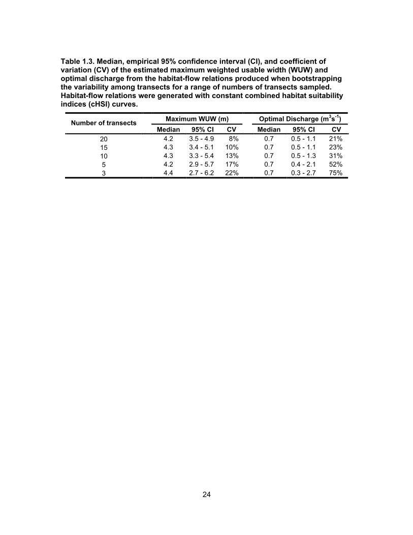
Figure 2.1. Hydrograph of the North Alouette River, BC, from 1970-2010, showing median daily discharge values (thick solid black line), upper/lower quartiles (solid grey lines) and minimum daily discharge (thin solid black line), and three low-flow benchmarks (0.25, 0.35, and 0.45 m3s-1) from Chapter 2 (dashed lines as indicated in the legend). ......... 64

Figure 2.2. The number of observed days (open circles) that discharge in the North Alouette River fell below (A) 0.45 m3s-1, (B) 0.35 m3s-1, and (C) 0.25 m3s-1 from 1970 to 2010, with multi-model averaged model predictions (thick solid line) and projections from 2011-2050 (thin black line with empirical 95% confidence interval grey band). ...................... 65

Figure 2.3. Observed summer mean daily temperature (ºC) (A), summer mean daily precipitation (mm) (B), and spring (April 1st) snowpack (cm) (C) in the North Alouette River watershed from 1970-2010 (open circles). Historical trends (thick black line) and future projections from 2011-2050 (thin black line with empirical 95% confidence interval grey band). ............................................................................................................ 66

Figure 2.4. The relative variable importance (RVI) of summer mean daily precipitation (P), spring snowpack (S), summer mean daily temperature (T), and interactions (P*S, P*T, and S*T) in explaining the number of days that discharge in the North Alouette River fell below (A) 0.45 m3s-1, (B) 0.35 m3s-1, and (C) 0.25 m3s-1 from 1970 to 2011. ............................................................................................................. 67

xiii

List of Acronyms

AIC Akaike Information Criterion

AICc Akaike Information Criterion with small sample size correction

BC British Columbia

BCIFM British Columbia Insteam Flow Methodology

cHSI Combined Habitat Suitability Index

CI Confidence Interval

CV Coefficient of Variation

ENSO El Nino-Southern Oscillation

GCM Global Circulation Model

HSI Habitat Suitability Index

IFR Instream Flow Requirement

MAD Mean Annual Discharge

PDO Pacific Decadal Oscillation

PHABSIM Physical Habitat Simulation Model

PNW Pacific Northwest

Q Discharge

ROR Run-Of-River

RVI Relative Variable Importance

SD Standard Deviation

SDU Standard Deviation Unit

WUW Weighted Usable Width

1

Chapter 1. General Introduction

The growing competition for water resources, coupled with a greater awareness

of the potential risks of discharge alterations to natural stream ecosystems, has placed

pressure on resource managers to improve water management. Of particular concern to

water resource managers are natural low-flow periods. During these critical periods,

many components of the natural aquatic ecosystem within the stream may be stressed;

hence, these periods are often assumed as limiting to productivity, especially for some

fish species (Poff and Zimmerman 2010). Resource managers frequently face the

difficult task of setting instream flow requirements (IFR) that allocate water during these

low-flow periods to industry, agriculture, and/or development, while also meeting

environmental objectives.

The stream discharge required to maintain aquatic ecosystem health has been a

question of concern faced by researchers across the globe for several decades

(Instream Flow Council 2002). As a result, many assessment methods have been

developed to assist resource managers in determining the IFR of rivers, from simple

desk-top based methods to more intensive field-based methods (Instream Flow Council

2002). However, not until recently has the uncertainty surrounding the results of any of

these assessment methods been critically evaluated (e.g., Williams 1996, 2010; Ayllón

et al. 2011). Understanding the uncertainty in the results of these assessment methods

is important because it can help to inform decision makers about the risks associated

with certain management actions. This type of informed decision making process has the

potential to improve the quality of water management decisions over time (Reckhow

1994).

In Chapter 2, I explore a common water management problem in British

Columbia (BC), Canada related to IRF. Management challenges related to IFR have

2

been accentuated in recent years with the emergence of run-of-the river (ROR)

hydroelectric project developments as a major component of BC’s energy policy. During

hydroelectric power generation, ROR facilities divert a portion of stream discharge out of

a stream channel, resulting in reduced discharge in a section of the stream. During the

permitting stages prior to construction of the facility, resource managers must make

decisions regarding the quantity of discharge that can be diverted from the channel for

hydroelectric power generation while minimizing impacts on fish and fish habitat. A

common instream flow assessment method used to determine IFR for these ROR

projects in BC is the British Columbia Instream Flow Methodology (BCIFM) (Lewis et al.

2004). The BCIFM is an empirical habitat-based assessment method that aims to

determine IFR for aquatic biota by assessing the habitat value of a reach of stream as a

function of discharge. Currently, however, decisions are often made regarding IFR by

water resource managers without considering many of the uncertainties in the BCIFM.

I explored how some particularly important uncertainties in the BCIFM influence

statistical confidence in the results, and how these uncertainties affect the chance of

habitat loss at different discharges for rainbow trout/steelhead (Oncorhynchus mykiss)

fry. I used a high-gradient reach of the North Alouette River, BC as a case study. I

presented the uncertain results of the BCIFM in terms of probability of habitat loss for a

given discharge, which can help managers set IFR based on their risk tolerance for fish-

habitat loss. Finally, based on the probabilities of certain magnitudes of habitat loss, I

inferred three potential IFR in the North Alouette River.

The projected rise in mean global temperature and changes in global weather

patterns associated with climate change (Intergovernmental Panel on Climate Change

2007) present yet another uncertainty to water resource managers. For the Pacific

Northwest of North America, global circulation models project changes in temperature,

precipitation patterns and type, timing of snowmelt, quantity of snowpack and glacial

runoff (Leith and Whitfield 1998; Morrison et al. 2002; Rodenuis et al. 2009; Elsner et al.

2010; Mote and Salathé 2010; Schnorbus and Rodenuis 2010; Schnorbus et al. 2011).

These variables have all been linked to shifts in stream discharge hydrographs, including

earlier spring runoff and prolonged summer low-flow periods (Leith and Whitfield 1998;

Morrison et al. 2002; Rodenuis et al. 2009; Elsner et al. 2010; Mote and Salathé 2010;

Schnorbus and Rodenuis 2010; Schnorbus et al. 2011). Anthropogenic water

3

withdrawals during these low-flow periods may be limited in order to salvage discharge

within the channel to maintain aquatic ecosystem health. Therefore, anticipating

changes in stream discharge resulting from climate change will be essential for

successful water resource management.

In chapter 3, I utilize a range of potential low-flow benchmarks that I identified in

chapter 2 for the North Alouette River, for which there were various probabilities of O.

mykiss fry habitat loss. I investigated how the number of days of low discharge in the

North Alouette River, BC, has changed from 1970 to 2010. I analyzed trends in

important weather variables including summer mean daily precipitation, summer mean

daily temperature, and spring mountain snowpack during this same period. I used these

three climate variables to model the number of days of low discharge each year using

multiple linear regression. Finally, I used simple projections of climate variables based

on historic rates of change to model trends in low discharge in the North Alouette River

from 2011 to 2050 and to suggest potential implications for the feasibility of ROR

hydroelectric generation as well as the health of natural stream ecosystems. These

types of predictive tools should help water resource managers incorporate the potential

effects of climate change into sustainable water management plans.

4

References

Ayllón, D., A. Almodóvar, G.G. Nicola and B. Elvira. 2011. The influence of variable habitat suitability criteria on PHABSIM habitat index results. River Research and Applications. doi: 10.1002/rra.1496.

Elsner, M.M., L. Cuo, N. Voisin, J.S. Deems, A.F. Hamlet, J.A. Vano, K.E.B. Mickelson, S.Y. Lee and D.P. Lettenmaier. 2010. Implications of 21st century climate change for the hydrology of Washington State. Climate Change. doi:10.1007/s10584-010-9855-0.

Instream Flow Council. 2002. Instream flows for riverine resource stewardship. The Instream Flow Council.

Intergovernmental Panel on Climate Change. 2007. Summary for Policymakers. Climate Change 2007: The Physical Science Basis. Contribution of Working Group I to the Fourth Assessment Report of the Intergovernmental Panel on Climate Change Cambridge University Press, Cambridge, United Kingdom and New York, NY, USA, 18 pp.

Lewis, A., T. Hatfield, B. Chilibeck and C. Roberts. 2004. Assessment methods for aquatic habitat and instream flow characteristics in support of applications to dam, divert, or extract water from streams in British Columbia. Prepared for: British Columbia Ministry of Sustainable Resource Management, and British Columbia Ministry of Water, Land, and Air Protection. Victoria, BC. URL:http://www.env.gov.bc.ca/wld/documents/bmp/assessment_methods_instreamflow_in_bc.pdf.

Leith, R.M.M. and P.H. Whitfield. 1998. Evidence of climate change effects on the hydrology of streams in south-central BC. Canadian Water Resources Journal 23:(3) 219-230. doi:10.4296/cwrj2303219.

Morrison, J., M.C. Quick and M.G.G. Foreman. 2002. Climate change in the Fraser River watershed: flow and temperature projections. Journal of Hydrology 263:230–244.

Mote, P.W., E.P. Salathé Jr. 2010. Future climate in the Pacific Northwest. Climate Change. doi:10.1007/s10584-010-9848-z.

Poff, N.L. and J.K.H. Zimmerman. 2010. Ecological responses to altered flow regimes: a literature review to inform the science and management of environmental flows. Freshwater Biology 55: 194-205. doi:10.1111/j.1365-2427.2009.02272.

Reckhow, K.H. 1994. Importance of scientific uncertainty in decision making. Environmental Management 18(2): 161-166.

5

Rodenhuis, D.R., K. Bennett, A. Werner, T. Murdock, and D. Bronaught. 2009. Hydro-climatology and future climate change impacts in British Columbia. Pacific Climate Impacts Consortium (PCIC), University of Victoria, and Victoria BC, 132 pp. URL: http://pacificclimate.org/sites/default/files/publications/Rodenhuis. ClimateOverview.Mar2009.pdf.

Schnorbus, M.A., K.E. Bennett, A.T. Werner and A.J. Berland. 2011. Hydrologic Impacts of Climate Change in the Peace, Campbell and Columbia Watersheds, British Columbia, Canada. Pacific Climate Impacts Consortium, University of Victoria, Victoria, BC. 157 pp.

Schnorbus, M., and D. Rodenhuis. 2010. Assessing Hydrologic Impacts on Water Resources in BC: Summary Report. Pacific Climate Impacts Consortium (PCIC). URL: http://pacificclimate.org/sites/default/files/publications/Schnorbus. BCHWorkshopReport.Aug2010.pdf.

Williams, J.G. 1996. Lost in space: minimum confidence intervals for idealized PHABSIM studies. Transaction of the American Fisheries Society 125: 458-465.

Williams, J.G. 2010. Lost in space, the sequel: spatial sampling issues with 1-D PHABSIM. River Research and Applications 26: 341-352.

6

Chapter 2. Evaluating Uncertainty in the British Columbia Instream Flow Methodology in a High-Gradient Mountain Stream

Introduction

The increasing demand for water resources has resulted in alterations in the

natural discharge of streams around the world, and the impacts of such discharge

alterations on river biota are well documented (e.g., Richter et al., 1997; Wills et al.,

2006; Dewson et al., 2007). Of particular importance is the human demand for diverted

water during periods of naturally occurring low discharge. The low-flow state in streams

is often recognized as a driver for changes in aquatic ecosystems (Bradford and

Heinonen 2008). During low-flow periods, most stream-habitat types experience a

reduction in habitat area, invertebrate production, and water quality, which can be

stressful for fish and other biota (Poff and Zimmerman 2010). As a result, resource

managers frequently face the difficult task of setting instream flow requirements (IFR)

that meet the needs of industry, agriculture, or other human activities, while also meeting

environmental objectives.

In British Columbia (BC), Canada, issues surrounding IFR were accentuated in

recent years with the emergence of run-of-the river (ROR) hydroelectric project

developments as a major component of British Columbia’s energy policy. ROR

hydroelectric projects are unique in that they use the natural discharge and gradient of a

stream to produce electricity without the construction of a major dam or reservoir (Paish

2002). A portion of the river’s discharge is diverted out-of-channel by an intake structure

and into a penstock. The water is transported down-slope to a powerhouse, where the

water turns turbines, generating electricity. The river water is subsequently returned to

7

the channel downstream from the powerhouse via a tail-race, restoring natural stream

discharge. Thus, the portion of the river channel between the intake structure and the

tailrace, which can extend for several kilometres, experiences reduced discharge. During

the permitting stages prior to construction of the facility, resource managers must make

decisions regarding the quantity of discharge that can be diverted from the channel for

hydroelectric power generation while minimizing impacts on fish and fish habitat.

The quantity of discharge required by aquatic biota has been a question of

concern faced by researchers across the globe for several decades (Instream Flow

Council 2002). As a result, many methods have been developed to assist resource

managers with setting IFR. Early methods included simple desk-top exercises that based

IFR on river characteristics, such as a percentage of the river’s mean annual discharge

(MAD) (e.g., Tennant’s method - Tennant 1976). More recently, habitat-based methods,

such as the physical habitat simulation model, PHABSIM (Bovee et al. 1998), or the

British Columbia Instream Flow Methodology (BCIFM) (Lewis et al. 2004), have been

used to assess the habitat value of a reach of stream as a function of discharge. In

general, these models predict the available habitat for a species of interest within the

stream from physical properties including water depth, velocity, bed material grain-size,

and sometimes cover type and abundance, each of them collected at transects on the

study stream. The transect data are weighted by biological models, or habitat suitability

indices (HSI), which describe the preferences, between 0 and 1, of the fish in terms of

the physical habitat variables (Williams 1996). Estimates of available habitat are either

measured or predicted at various discharges; these estimates can be fit with a curve to

characterize the change in available habitat with change in discharge, referred to here

as the habitat-flow relation.

Although PHABSIM is one of the most widely used instream flow assessment

methods (Ayllon et al, 2011), provincial instream flow guidelines in BC recommend the

use of the BCIFM as a primary assessment method for water diversion projects such as

small hydropower developments (Lewis et al. 2004). This empirical, habitat-based

assessment method is similar to PHABSIM in that it uses physical habitat data from

multiple transects to estimate a habitat-flow relation based on habitat preferences of

target organisms. However, instead of using a hydraulic model to estimate the physical

habitat conditions along a reach of a river, as in PHABSIM, the BCIFM requires field

8

measurements of physical habitat variables from multiple transects at multiple

discharges to produce an empirical estimate of a habitat-flow relation.

However, like PHABSIM, the BCIFM was developed without an explicit method

for accounting for uncertainties in the analysis. It is now recognized that uncertainties in

such habitat-based instream flow studies are large and ubiquitous (Williams 1996, 2010,

Ayllón et al. 2011). Measurement error, variation in physical habitat variables among

transects and different discharge levels, uncertainties in HSI curves of a given species,

and inaccuracies in hydraulic models all contribute to uncertainty in the results of habitat-

based instream flow assessment methods (Williams 1996). Using PHABSIM and variant

models, researchers have begun to examine how incorporating uncertainty in HSI

curves affects the resulting habitat-flow relation (Ahmadi-Nedushan et al. 2008; Mouton

et al. 2008, 2011; Fukuda 2009, Ayllón et al. 2011). Others have explored how the

variation among, and the number of, transects affects the uncertainty in the habitat-flow

relation produced by PHABSIM (Williams 1996, 2010; Ayllón et al. 2011). However,

these two important sources of uncertainty have yet to be rigorously explored using the

BCIFM. This is the gap that my research aims to fill.

For many instream assessment projects, budgets or time may be limiting.

Therefore, it is important to understand where the largest uncertainties lie in order to set

priorities for sampling efforts. Efforts can be divided between the collection of HSI data

and transect data. Often, these budget/time limitations may restrict the number of

transects used in the analysis. Therefore, it is important to understand how the accuracy

of estimates increases with the number of transects used in the analysis. In addition,

data for developing HSI curves specific to individual streams may not be collected

because of these budget/time limitations, forcing instream flow practitioners to choose

between multiple pre-existing sets of HSI curves to conduct the analysis for a given

species. Often there is considerable variation among these pre-existing sets of HSIs that

potentially produce different outcomes in the habitat-flow relation (Williams et al. 1999).

This uncertainty in the choice of HSI curves presents another unresolved uncertainty in

habitat-based instream flow assessment methods that is important to consider when

setting sampling effort priorities.

9

Because habitat-flow relations are used directly by water resource managers to

infer IFR of streams, both Williams (1996) and Hatfield et al. (2007) insist that statistical

confidence intervals be presented on these habitat-flow relations. To aid in the

interpretation of these confidence intervals, the uncertainty in the habitat-flow relation

should be presented in a manner in which managers can choose IFR based on the

probability of habitat loss. In doing so, managers can make decisions informed by their

risk tolerance.

Therefore, I had four main research objectives: (1) explore how uncertainty in

choice of fish HSI curves affects uncertainty in the resulting habitat-flow relation

produced by the BCIFM; (2) examine how the level of uncertainty in the habitat-flow

relation is affected by variation in physical habitat among the sampled transects, and

how that variation changes with the number of transects; (3) demonstrate the relative

contribution of each of these two sources of uncertainty to the total uncertainty in the

habitat-flow relation; and (4) show how the uncertainty in the habitat-flow relation

translates into uncertainty about habitat loss for a given discharge. These results can be

used to explore, and communicate to managers, the uncertainty in the habitat-flow

relation produced by the BCIFM.

Methods

Field Site

The North Alouette River (49°15’50”N, 122°34’00”W) flows out of the Golden

Ears mountain range and drains into the Pitt River near the town of Maple Ridge, British

Columbia, Canada (Figure 1.1). The watershed is located within the coastal temperate

rainforest region, which is characterized by dry summers with low discharge and wet

winters with heavy rainfall events that cause sporadic high discharge. My study site was

located directly above a waterfall complex, within the University of British Columbia

Malcolm Knapp Research Forest approximately 15 km upstream from the confluence

with the Pitt River.

The North Alouette River has a total drainage area of 37.3 km2 with a mean

annual discharge of 2.8 m3s-1 (Environment Canada 2011). The channel of the study

10

reach was high-gradient (2.0-3.1%), with an average channel width of 18.6 m. The study

reach was dominated by boulder, cobble, and gravel bed material with a D50 and D90 bed

material grain size ranging from 130-180 mm and 400-430 mm respectively (obtained

using Wolman pebble counts; Kondolf 1997). The study reach was exclusively

composed of plane bed alluvial channel type (Montgomery and Buffington 1997) with

riffle-run mesohabitat type (Maddock 1999). A waterfall complex downstream of the

study site prevents the upstream migration of anadromous salmonids into the study

reach. However, rainbow trout (Oncorhynchus mykiss) and cutthroat trout (O. clarkii)

were introduced into the system in the mid-19th century and currently inhabit the reach

(Mathes and Hinch 2009).

Physical Habitat Data

I collected physical habitat data from the North Alouette River on 5 dates during

the summer and fall of 2010. I established two sets of 10 cross-stream transects (n=20).

The first set of transects was systematically spaced 10 m apart from random starting

points. The second set of transects was identical but was located approximately 250 m

upstream from the first set. Transects were placed perpendicular to the stream flow and

marked either with 1-m rebar stakes pounded into the river bed or 15-cm metal spikes

tacked into trees adjacent to the stream bank. Measurements of river physical habitat

(depth, velocity, width, and bed-material grain size) were collected at 0.5-m increments

along each transect, as outlined in the BCIFM (Lewis et al. 2004). Depth and velocity

measurements were collected using a wading rod and Marsh-McBirney Flo-Mate™.

River discharge was calculated each day that physical data were collected from a

designated transect as outlined in Resources Information Standards Committee (2009).

The discharges sampled were: 0.13, 0.28, 0.55, 1.46, and 1.79 m3s-1. I calculated the

mean annual discharge (MAD) from 40 years of mean daily discharge data from a Water

Survey of Canada gauging station approximately 3 km downstream of the study reach

(Environment Canada 2011).

Habitat Preference Data

In order to describe uncertainty in habitat preferences of an aquatic organism, I

compiled results from several studies of habitat suitability indices (HSI) for O. mykiss fry

11

in North America. In total, five sets of HSI curves for depth and velocity were gathered

(Figure 1.2). To simplify the analysis, uncertainty in habitat preferences for bed-material

grain size was not considered; instead I used a universal set of bed-material preferences

for O. mykiss fry (Figure 1.3).

Habitat-Flow Relation

Physical habitat data and HSI information were combined to produce a metric of

availability of habitat for O. mykiss fry, weighted usable width (WUW) (Lewis et al. 2004)

at each transect at each discharge as:

, (1)

where the WUW of each transect is the sum of the WUW of all n cells. The

WUW of each cell, i, is calculated as its width (wi) multiplied by its suitability of depth

(dHSIi), velocity (vHSIi), and substrate size (sHSIi).

The habitat-flow relation was estimated for the study reach by fitting a log-normal

function with a multiplicative scalar to the WUW vs. discharge data. This log-normal form

is typical of habitat-flow relations (Lewis et al. 2004). The reach average WUW was thus

calculated as:

, (2)

where the WUW is a function of discharge (Q), a scalar (A), a location parameter

(µ) and a scale parameter (σ). The log-normal function was fit to WUW-discharge data

using a least-squares optimizing function in R (R Development Core Team 2008).

Fitting the habitat-flow relation with this log-normal function allowed me to solve

for important management parameters in the study reach. These parameters were (1)

the maximum WUW, which was the maximum amount of habitat available at the peak of

the habitat-flow relation, (2) the optimal discharge, which is the discharge at which the

maximum WUW occurs, and (3) the discharges at which different percentages of habitat

loss occurred on the ascending limb of the habitat-flow relation relative to the maximum

12

WUW. All management parameters were calculated numerically using a maximum

optimizing function in R (R Development Core Team 2008).

HSI Uncertainty

I first evaluated the effect of the choice of HSI set on the resulting habitat-flow

relation from the BCIFM and the corresponding management parameters. Habitat-flow

relations were generated and management parameters were calculated for each of the

five different sets of HSI curves for depth and velocity using physical habitat data from

the 20 transects at five discharge values.

As an alternative to selecting a single set of HSI depth and velocity curves, I

combined the 5 sets of HSI curves into single curves for depth and velocity, under the

assumption that each of the 5 sets of HSI curves (Figure 1.2) were equally likely. These

combined HSI curves for depth and velocity, denoted as cHSI, were calculated by

dividing the 5 individual curves into intervals of 0.01 m·s-1 for velocity and 0.01 m for

depth. The habitat preference for depth and velocity at each interval was calculated by

randomly sampling the five habitat preference values from my set of HSI curves with

replacement and calculating the mean value of the sample. This process was repeated

1000 times. Uncertainty in cHSI curves was expressed as the median, 2.5 and 97.5%

quantiles of the bootstrap samples for each interval. A sixth habitat-flow relation (cHSI)

was generated from the resulting medians for each interval.

To evaluate the uncertainty in the habitat-flow relation resulting from uncertainty

in the cHSI curves, I generated a habitat-flow relation from each bootstrap sample of the

combined HSI curves for depth and velocity (Figure 1.4). This resulted in the generation

of 1000 habitat-flow relations and corresponding management parameters for which the

median, empirical 95% confidence interval (CI), and coefficient of variation (CV) were

calculated.

Physical Habitat Uncertainty

As an indication of variability in physical habitat between sampled transects, I

plotted the relation between river discharge and channel width, mean depth, and mean

velocity among the 20 sampled transects in the North Alouette River. The relations for

13

individual transects were fit with power functions according to rules of at-a-station

hydraulic geometry (Leopold 1953).

I used a bootstrap analysis (Efron and Tibshirani 1993) to develop uncertainty

bounds on the habitat-flow relation resulting from the variability in physical habitat

among transects (Figure 1.4). I calculated available habitat at each transect at each

discharge by fixing the HSI curves as the median of the cHSI curves for depth and

velocity. I assumed that each transect could be treated as an independent sample of

stream habitat. For each bootstrap iteration, 20 transects were randomly sampled with

replacement. WUW was calculated for each of the bootstrap samples, a habitat-flow

relation was generated, and management parameters were calculated. This process was

repeated 1000 times. Again, the median, empirical 95% CI, and CV of the resulting

management parameters from those 1000 bootstrap samples were calculated.

In addition, the uncertainty in the habitat-flow relation resulting from physical

habitat variability among transects was assessed as a function of the number of

transects used in the analysis. The sample size of the randomly drawn transects was

reduced incrementally from 20 to 3 in separate analyses. For each sample size,

transects were randomly sampled with replacement. WUW was calculated for each of

the bootstrap samples, a habitat-flow relation was generated, and management

parameters were calculated. This process was repeated 1000 times for each increment

in transect sample size. The median, empirical 95% CI, and CV of the resulting

management parameters were calculated.

Combined Uncertainty

I used another bootstrap analysis to develop uncertainty bounds on the habitat-

flow relation resulting from the combination of uncertainty in the estimate of the cHSI

curve and transect variability (Figure 1.4). For each bootstrap sample, 20 transects were

randomly sampled with replacement. For each of those 20 transects, WUW was

calculated at each discharge level using a set of HSI curves randomly sampled from the

cHSI curves. A habitat-flow relation was generated and management parameters were

calculated. This entire process was repeated 1000 times and the median, empirical 95%

CI, and CVs of the resulting management parameters were calculated.

14

Habitat Loss

Using the habitat-flow relations produced from the analysis that incorporated the

combination of uncertainty in the estimate of the cHSI curve and variability in physical

habitat among transect, I calculated both the percent habitat loss (median and 95% CI)

and the probability of a particular magnitude (0, 5, 10, and 25%) of habitat loss occurring

as a function of discharge. I defined habitat loss as the percent decrease in WUW

relative to the maximum WUW. Habitat loss was only considered on the ascending limb

of the habitat-flow relation because habitat losses occurring from high discharges were

of little concern when considering minimum discharge requirements for a stream.

Results

HSI Uncertainty

In the study reach of the North Alouette River, the use of different sets of HSI

curves for depth and velocity for O. mykiss fry (Figure 1.2) produced substantially

different habitat-flow relations (Figure 1.5). Management parameters calculated from

each of the habitat-flow relations reflected those differences (Table 1.1).

Uncertainty in habitat preferences by O. mykiss fry, as reflected by uncertainty in

the estimate of the cHSI curve (Figure 1.6), resulted in substantial uncertainty in the

habitat-flow relation (Figure 1.7A). This uncertainty was reflected in both the maximum

weighted useable width (WUW) and the optimal discharge (Table 1.2).

Physical Habitat Uncertainty

Variability in the relation between river discharge and channel width, mean depth,

and mean velocity among the 20 sampled transects in the North Alouette River is shown

in Figure 1.8. Although substantial, variation among sampled transects through the

BCIFM generated less uncertainty about the shape of the habitat-flow relation than did

the choice of HSI curve (Figure 1.7B). For this effect of transect alone, uncertainty was

greater for the optimal discharge parameter than the maximum WUW parameter (Table

1.2). However, when the number of transects used in the analysis was reduced from 20,

the magnitude of uncertainty about both parameters increased at an accelerating rate

15

(Table 1.3). In particular, when small numbers of transects were used in the analysis

(<15), variability among those transects resulted in substantial uncertainty in estimates

of the optimal discharge parameter.

Combined uncertainty

When both variability in physical habitat among sampled transects and

uncertainty in the estimated cHSI curves were combined, the uncertainty in the habitat-

flow relation increased in an additive manner compared to when either source of

variability was incorporated independently (Figure 1.7C). This additive increase in

uncertainty about the habitat-flow relation was reflected in the CVs of management

parameters (Table 1.2).

Habitat Loss

Habitat loss, as calculated from the habitat-flow relation that incorporated the

combination of both variability in physical habitat among sampled transects and

uncertainty in the estimated cHSI curves, increased non-linearly with decreasing

discharge values (Figure 1.9). At discharge values of below approximately 0.45 m3s-1, it

was highly likely that at least some habitat loss will occur for O. mykiss fry, and the

percent habitat loss increased at an accelerating rate with decreasing discharge.

In addition, I calculated the probability of different magnitudes of habitat loss as a

function of discharge (Figure 1.10). The probability of a given magnitude of habitat loss

increased nonlinearly with decreasing discharge values. This nonlinear increase resulted

in threshold discharge values for each magnitude of habitat loss at which the probability

of that habitat loss began to increase dramatically as discharge decreased. A 0% habitat

loss is equivalent to the optimal discharge from the habitat-flow relation; therefore, this

line in Figure 1.10 can be interpreted as the probability that any habitat loss will occur.

For example, at a discharge of 0.45 m3s-1, there is a probability of approximately 0.95

that less than 5% habitat loss will occur. For larger magnitude losses (5-25%), the figure

can be interpreted as the probability that the given magnitude of habitat loss will occur.

For example, at a discharge of 0.25 m3s-1, there is a probability of approximately 0.05

that a 25% habitat loss will occur but >95% chance that a 10% loss will occur.

16

Discussion

Evaluating Uncertainty

I found that both variability among transect samples and uncertainty in habitat

preference data were important when generating a habitat-flow relation using the British

Columbia Instream Flow Methodology (BCIFM). Further, I estimated the relative

importance of each source of uncertainty. The uncertainty from the HSI curves is very

important when large numbers of transects are used in the analysis; however, when

small numbers of transect are used (<15), the variation in physical habitat among

transects becomes a dominant source of uncertainty in the analysis, particularly in

estimates of the optimal discharge. This information is important to instream flow

practitioners who are limited by budget/time constraints and who must strategically focus

sampling efforts. One novel aspect of this work is how I interpret uncertainty in the

habitat-flow relation. Specifically, I express results of the BCIFM in terms of probability of

different magnitudes of habitat loss. Such probabilities can be used by decision makers

to set instream flow requirements (IFR) based on their individual risk tolerance for habitat

loss.

In this study, I simulated a scenario in which instream flow practitioners may be

forced to choose among multiple pre-existing sets of HSI curves because budget or time

limitations do not allow them to develop location-specific curves. As an example, I

collected five sets of curves describing O. mykiss fry depth and velocity preferences that

contained considerable variation among results (Figure 1.2). In general, the most

pronounced differences in the HSI curves were habitat preferences for higher velocities.

Some curves suggest that fry begin to lose preference for water velocities greater than

0.1 m·s-1 (e.g., HSI curve-B and C), whereas other curves suggest preferences do not

drop until water velocities reach greater than 0.45 m·s-1 (e.g., HSI curve-C). In addition,

curves varied greatly in preferences of fry for different water depths. Some curves show

substantially higher preferences for deeper water (e.g., HSI curves C and D), whereas

others show higher preferences for shallow water (e.g., HSI curves A and D).

This variation among sets of HSI curves for O. mykiss fry may be attributed to

several factors. The methods used to generate the HSI curves vary between studies,

17

from field data collection to expert-opinion-driven processes. In addition, variation among

HSI curves can result from natural variability in habitat preferences of O. mykiss fry

(Williams et al. 1999). Genetic variability among isolated populations of the same

species may result in variability in habitat-preferences because of behavioural

adaptation to local conditions. Alternatively, variability in habitat preferences for depth

and velocity can result from fluctuations in other physical variables such as discharge

(Beecher et al. 1995), season (Yu and Peters 2002), light intensity (Rowe and Chisnall

1995, Metcalfe et al. 1997), temperature (Rowe and Chisnall 1995), and dissolved

oxygen (Kramer 1987, Rowe and Chisnall 1995).

Regardless of the source of variation among the different sets of depth and

velocity HSI curves, I found that the use of these different sets of HSI curves had a large

influence on the habitat-flow relation, which could have serious management

implications. In general, velocity preferences of O. mykiss fry played a more pronounced

role in determining the maximum WUW and optimal discharge than did depth

preferences in the North Alouette River because water velocities often exceeded

preferences, whereas water depths did not (Figure 1.2 and 1.8). As a result, those sets

of HSI curves that contained higher habitat preferences for low water velocities tended to

produce habitat-flow relations with a lower maximum WUW and optimal discharge. Such

sets of HSI curves will result in IFR curves biased towards lower discharge values, which

could potentially put fish habitat at risk of loss if the HSI curves were incorrect. It is

important to note, however, that in slower moving, deeper rivers, depth preferences may

be more important than velocity preferences. In such rivers, HSI curves with higher

preferences for low water depths may result in IFR choices biased towards lower-than-

ideal discharge values for the protection of aquatic habitat.

As an alternative to choosing a single set of HSI curves and producing potentially

biased results, I explored a method that produced combined HSI (cHSI) curves for depth

and velocity. This method allowed me to incorporate variation among the pre-existing

sets of HSI curves into the estimates of the habitat-flow relation through the BCIFM. In

this example, because I had no basis to prefer one curve over another, I assumed each

competing curve was equally likely. Other weighting schemes could be used if there was

reason to choose or prefer one or some over others. In addition, other methods exist to

quantify the uncertainty in habitat preferences of organisms on a regional or local scale,

18

such as uncertainty bounds of univariate resource selection functions (Ayllón et

al.(2011), expert opinion (Johnson and Gillingham 2004), and fuzzy logic (Burgman

2001; Ahmadi-Nedushan et al. 2008; Mouton et al. 2008 and 2011; Fukuda 2009).

Incorporation of the uncertainty in the estimated cHSI curves alone through the

BCIFM resulted in considerable uncertainty in the habitat-flow relation, which translated

into substantial uncertainty in estimates of the management parameters, particularly in

the maximum WUW parameter. The large amount of uncertainty about the upper

tolerance limits of the cHSI curves for depth and velocity (e.g., where habitat preference

scores fall below 0.5) likely resulted in the large uncertainty in the habitat-flow relation.

Small differences in depth and velocity preferences around these upper tolerance limits

substantially changed the amount of available habitat in the study reach because those

upper tolerances for both depth and velocity were often exceeded in some portions of

the river, even at low discharges.

When the full set of 20 transects was used in the analysis, variability in physical

habitat among transects translated into relatively little uncertainty in the maximum WUW

parameter and roughly equal uncertainty in the optimal discharge compared to that

arising from the uncertainty in the estimated cHSI curves. The manner in which the

physical habitat (depth, velocity, and width) of a transect changes with discharge, also

known as the at-a-station hydraulic geometry (Leopold 1953), governs the shape of the

habitat-flow relation in conjunction with the habitat preferences of the organism. Because

of the relatively homogenous river morphology over the study reach of the North

Alouette River, the at-a-station hydraulic geometry remained fairly constant among

transects. Rivers with more variable morphology (i.e., riffle-pool sequences) and bed-

material grain size will have more variable at-a-station hydraulic geometry and thus

transect data will be more variable. This increased variability will result in more

uncertainty in the habitat-flow relations, especially in optimal discharge estimates.

Variability in management parameters from the habitat-flow relation increased

nonlinearly as the number of transects used in the analysis decreased (Table 1.3). Both

variability in the maximum WUW and the optimal discharge did not increase dramatically

when reducing the number of transects from 20 to 15. However, for fewer transects than

15, uncertainty increased substantially and was a dominant source of uncertainty in the

19

analysis, particularly in the estimates of optimal discharge. This result suggests that, for

streams with similar characteristics to the North Alouette River, a minimum of 15

transects should be used to minimize variability in transect data when conducting a

BCIFM analysis. However, for more than 15 transects, the increase in information

(decrease in variability) is not likely worth the effort of collecting the physical habitat data

in reaches with homogeneous morphology and bed material grain-size. This number is

on the lower end of the 15-20 transects suggested in the literature to be used to capture

the full variability of rivers and produce a meaningful habitat-flow relation using

PHABSIM (Williams 1996; Thomas et al. 2004). It is likely that because of the lack of

heterogeneity in the river morphology of the North Alouette River, a smaller number of

transects was needed to sufficiently capture the variability in physical habitat.

Habitat Loss

Uncertainty in the habitat-flow relation can be interpreted by investigating the

percent habitat-loss and the probability of certain magnitudes of habitat-loss occurring as

a function of discharge. Calculating the percent habitat loss (with 95% empirical

confidence intervals) will allow managers to analyse where habitat loss is likely to occur.

In the North Alouette River, discharge levels below 0.45 m3s-1 likely result in loss of

habitat to O. mykiss fry relative to the optimal discharge, and the percent habitat loss

increases at an accelerating rate with decreasing discharges below that value (Figure

1.9). Calculating the probability of different magnitudes of habitat loss as a function of

discharge allows managers to target a specific discharge value based on an acceptable

probability for a given magnitude of habitat loss occurring (Figure 1.10). In addition,

threshold discharge values become evident where the probability of a particular

magnitude of habitat loss increases rapidly with decreasing discharge values. These

threshold discharge values could be relevant because water resource managers could

use them as cut-off points to define discharge levels to be avoided because of their

undesirable magnitudes of habitat loss. For example, if a manager desired to have less

than a 5% loss of O. mykiss fry habitat in the North Alouette River, he or she would

recommend an instream flow requirement of at least 0.45 m3s-1, at which there is a

probability of 0.95 of having less than 5% habitat loss. In contrast, if a manager was

willing to take a chance of losing some habitat but wanted to avoid large magnitudes of

habitat loss to O. mykiss fry habitat, an instream flow requirement of at least 0.25 m3s-1

20

would be advised, where there is a probability of approximately 0.05 that a 25% habitat

loss will occur.

Conclusion

Understanding the relative contributions of uncertainty to the results of the

BCIFM is important in order to set priorities for sampling efforts. If budgets/time are

limiting, my results suggested that priority should be taken to collect physical habitat

data from at least 15 transects in order to capture adequate variability of stream

morphology, providing the river has similar morphology and bed material grain-size

throughout the reach of interest. Regardless of the transect-based instream flow

assessment method used by practitioners (e.g., PHABSIM or BCIFM), this finding should

hold true, because the aim of transect sampling is to capture sufficient variability of the

physical environment within a river.

My results demonstrated the importance of including uncertainty in habitat

preferences of an organism when developing a habitat-flow relation. I showed that

instead of developing data-intensive, stream-specific habitat preferences for a species of

interest, composites of pre-existing HSI curves could be used to estimate uncertainty in

habitat preferences of that organism. This method would be especially advantageous if

budgets or time are very limiting. However, if funds and time were available, generation

of a stream- and species-specific HSI may reduce uncertainty in the recommended

instream flow requirements (IFR).

Finally, my results showed that when uncertainty is incorporated in the habitat-

flow relation, calculating the probability of different magnitudes of habitat loss permitted

clear and concise interpretation and communication of this uncertainty. This information

is important because it allows managers to develop IFR based on their risk tolerance for

habitat loss. Without this sort of information, managers are left to set IFR based on best

point estimates of available habitat as a function of discharge, with little knowledge of the

certainty of maintaining the aquatic ecosystem’s health.

However, one should also be cautious when extrapolating the results of this

study to other river systems or other species. Because the current findings are limited to

21

the river, reach, and species of study, generalizations of these findings must be checked

by repeating similar sampling and statistical analysis on rivers of different scales, slopes,

and morphologies, and with species with different habitat preferences. In addition, many

uncertainties and assumptions of habitat-based assessment methods were not

considered in this study. For example, I collected physical habitat data from the North

Alouette River at five different discharge levels. Although it was not considered in this

study, the ideal number of sample discharge values across which these physical habitat

conditions should be collected needs to be explored in order to further set priorities for

sampling efforts.

22

Tables

Table 1.1. Estimated maximum weighted usable width (WUW) and optimal discharge from the habitat-flow relation produced by each of the five habitat preference curves (A-E) and the combined HSI (F). Habitat-flow relations shown in Figure 1.5. Letter correspond to the habitat preference curves from Figure 1.2.

HSI curve set Maximum WUW (m) Optimal Discharge (m3s-1) A 6.3 0.4 B 1.5 0.8 C 8.7 1.1 D 3.3 1.0 E 3.3 0.4 F 4.3 0.7

23

Table 1.2. Median, empirical 95% confidence interval (CI), and coefficient of variation (CV) of the estimated maximum weighted usable width (WUW) and optimal discharge from the habitat-flow relations produced when incorporating (1) uncertainty from the combined habitat suitability indices (cHSI) with the transects fixed, (2) variability among transects but using a constant cHSI, and (3) both sources of uncertainty. Habitat-flow relations shown in Figure 1.7.

Maximum WUW (m) Optimal Discharge (m3s-1) Source of Uncertainty

Median 95% CI CV Median 95% CI CV cHSI 4.3 2.5 - 6.8 25% 0.7 0.5 - 1.0 21% Transect 4.2 3.5 - 4.9 8% 0.7 0.5 - 1.1 21% cHSI & Transect 4.3 2.3 - 6.8 27% 0.7 0.4 - 1.3 34%

24

Table 1.3. Median, empirical 95% confidence interval (CI), and coefficient of variation (CV) of the estimated maximum weighted usable width (WUW) and optimal discharge from the habitat-flow relations produced when bootstrapping the variability among transects for a range of numbers of transects sampled. Habitat-flow relations were generated with constant combined habitat suitability indices (cHSI) curves.

Maximum WUW (m) Optimal Discharge (m3s-1) Number of transects Median 95% CI CV Median 95% CI CV

20 4.2 3.5 - 4.9 8% 0.7 0.5 - 1.1 21% 15 4.3 3.4 - 5.1 10% 0.7 0.5 - 1.1 23% 10 4.3 3.3 - 5.4 13% 0.7 0.5 - 1.3 31% 5 4.2 2.9 - 5.7 17% 0.7 0.4 - 2.1 52% 3 4.4 2.7 - 6.2 22% 0.7 0.3 - 2.7 75%

25

Figures

Figure 1.1. Study area (oval) on the North Alouette River, BC (Modified from Mathes and Hinch 2009).

26

Figure 1.2. Functions for habitat preference for O. mykiss fry for depth (top panel) and velocity (bottom panel). Data were drawn from five studies as indicated in the legend, except (F) cHSI, which is the median of the bootstrapped mean of the 5 habitat preference curves (A-E).

27

Figure 1.3. Functions for habitat preferences for O. mykiss fry for bed-material type used across all analyses. Substrate categories refer to detritus (Dt), silt (Sl), sand (Sn), gravel (Gr), cobble (Cb), rubble (Rb), small boulders (SB), large boulders (LB), and bedrock (BR). From Ptolemy, R., pers. comm., 2011, Rivers Biologist, Fisheries Science Section, Ecosystems Branch, Ministry of Environment, Victoria, BC.

28

Figure 1.4. Flow diagram of the method used to incorporate the uncertainties of the habitat suitability indices (HSI) and transect data into the habitat-flow relation produced by the British Columbia Instream Flow Methodology (BCIFM).

29

Figure 1.5. Results of the sensitivity analysis showing the estimated habitat-flow relations for O. mykiss fry in the North Alouette River for the six sets of habitat preference curves for depth and velocity presented in Figure 1.2. Letters correspond to habitat preference curves A-F in Figure 1.2. Open circles are weighted usable width calculations for each of the 20 transects at the five discharge levels. The solid line is the fit of the log-normal function (equation 2).

30

Figure 1.6. Combined habitat suitability indices (cHSI) for O. mykiss fry for depth (top panel) and velocity (bottom panel). The solid line is the median and grey band is the empirical 2.5 and 97.5% confidence interval from bootstrapping the mean of five habitat suitability indices in Figure 1.2. Bootstrapped means were generated at 0.01 intervals along the x axis.

31

Figure 1.7. Estimated habitat-flow relations produced by the BCIFM when integrating the uncertainty from (A) the combined habitat suitability indices (cHSI) (Figure 1.6), (B) the variability among transects while using a constant cHSI for depth and velocity, and (C) both sources combined. Solid line is the median weighted usable width; grey band is the empirical 2.5 and 97.5% confidence interval from a bootstrap analysis.

32

Figure 1.8. Variability in the relation between river discharge and width, mean depth, and mean velocity among the 20 sampled transects in the North Alouette River (open circles). The relations for individual transects were fit with a power function (grey line) according to rules of at-a-station hydraulic geometry (Leopold 1953).

33

Figure 1.9. Estimated habitat loss from the maximum for O. mykiss fry in the North Alouette River as a function of discharge. The solid line is the median value; grey band is the empirical 95% confidence interval from a bootstrap analysis. Uncertainty in both combined habitat suitability indices (cHSI) and transect data were included. The figure presents habitat losses occurring only on the ascending limb of the habitat-flow relation.

34

Figure 1.10. Estimated probability of habitat loss for O. mykiss fry in the North Alouette River as a function of discharge. Magnitude of habitat loss (0, 5, 10, and 25%) are presented as different line types. The habitat-flow relations that data were drawn from incorporated both uncertainty in (combined habitat suitability indices) cHSI and transect data (Figure 1.7C). This figure presents results from the analysis of habitat loss only on the ascending limb of the habitat-flow relation.

35

References

Addley, C., G.K. Clipperton, T. Hardy and A.G.H. Locke. 2003. South Saskatchewan River Basin, Alberta, Canada - Fish Habitat Suitability Criteria (HSC) Curves. Alberta Fish and Wildlife Division, Alberta Sustainable Resource Development. Edmonton, Alberta. 63 pp. ISBN 0-7785-359-4.

Ahmadi-Nedushan, B., A. St-Hillaire, M. Berube, T.B.M.J. Ouarda and E. Robichaud.2008. Instream flow determination using a multiple input fuzzy-based rule system: a case study. River Research and Applications 24: 279-292.

Ayllón, D., A. Almodóvar, G.G. Nicola and B. Elvira. 2011. The influence of variable habitat suitability criteria on PHABSIM habitat index results. River Research and Applications. doi: 10.1002/rra.1496.

Beecher, H.A., J.P. Carleton, and T.H. Johnson. 1995. Utility of depth and velocity preferences for predicting steelhead parr distribution at different flows. Transactions of the American Fisheries Society 124: 935-938.

Bovee, K. D. 1978. Probability-of-use criteria for the family Salmonidae. Instream Flow Inf. Pap. 4. U.S. Fish and Wildlife Service. FWS/OBS-78/07. 80 pp.

Bovee, K.D., B.L. Lamb, J.M. Bartholow, C.B. Stalnaker, J. Taylor and J. Henriksen. 1998. Stream habitat analysis using the instream flow incremental methodology. U.S. Geological Survey, Biological Resources Division Information and Technology Report USGS/BRD-1998-0004. viii + 131 pp.

Bradford, M. J. and J. S. Heinonen. 2008. Low flows, instream flow needs and fish ecology in small streams. Canadian Water Resources Journal 33:165-180.

Burgman, M.A., D.R. Breininger, B.W. Duncan and S. Ferson. 2001. Setting reliability bounds on habitat suitability indices. Ecological Applications 11(1): 70-78.

Dewson, Z.S., A.B.W. James and R.G. Death. 2007. Invertebrate responses to short-term water abstraction in small New Zealand streams. Freshwater Biology 52:357-369.

Environment Canada. 2011. Water Survey of Canada: North Alouette River at 232nd Street, Maple Ridge, BC. (08MH006). URL: http://www.wsc.ec.gc.ca.

Efron, B. and R. Tibshirani. 1993. An introduction to the bootstrap. Chapman and Hall. New York.

Fukuda, S. 2009. Consideration of fuzziness: Is it necessary in modelling fish habitat preference of Japanese medaka (Oryzias latipes). Ecological Modelling 220: 2877-2884.

36

Hatfield, T., A. Lewis, and Babakaiff. 2007. Guidelines for the collection and analysis of fish and fish habitat data for the purpose of assessing impacts from small hydropower projects in British Columbia. Prepared for: British Columbia Ministry of Sustainable Resource Management, and British Columbia Ministry of Water, Land, and Air Protection. Victoria, BC.

Higgins, P.S., J.G. Scouras, and A. Lewis. 1999. Diurnal and nocturnal microhabitat use of stream salmonids in Bridge and Seton Rivers during summer. Consultant's report prepared for BC Hydro, Strategic Fisheries. 26 p. + App.

Instream Flow Council. 2002. Instream flows for riverine resource stewardship. The Instream Flow Council.

Johnson, C.J. and M.P. Gillingham. 2004. Mapping uncertainty: sensitivity of wildlife habitat ratings to expert opinion. Journal of Applied Ecology 41: 1032-1041.

Kondolf, G.M. 1997. Application of the pebble count notes on purpose, method, and variants. Journal of the American Water Resources Association 33(1): 79–87.

Kramer, D.L. 1987. Dissolved oxygen and fish behavior. Environmental Biology of Fishes 18(2): 81-92.

Leopold, L.B. and T. Maddock Jr. 1953. The hydraulic geometry of stream channels and some physiographic implications. US Geological Survey Professional Paper 252, 56p.

Lewis, A., T. Hatfield, B. Chilibeck and C. Roberts. 2004. Assessment methods for aquatic habitat and instream flow characteristics in support of applications to dam, divert, or extract water from streams in British Columbia. Prepared for: British Columbia Ministry of Sustainable Resource Management, and British Columbia Ministry of Water, Land, and Air Protection. Victoria, BC. URL:http://www.env.gov.bc.ca/wld/documents/bmp/assessment_methods_instreamflow_in_bc.pdf.

Maddock, I. 1999. The importance of physical habitat assessment for evaluating river health. Freshwater Biology 41: 373-391.

Metcalfe, N.B., S.K Valdimarsson, and N.H.C. Fraser. 1997. Habitat profitability and choice in a sit-and-wait predator: juvenile salmon prefer slower currents on darker nights. Journal of Animal Ecology 66: 866-875.

Mathes, M.T. and S.G. Hinch. 2009. Stream flow and fish habitat assessment for a proposed run-of-the-river hydroelectric power project on the North Alouette River in the Malcolm Knapp Research Forest. Unpublished Manuscript, University of British Columbia, BC, Canada.

Montgomery, D.R. and J.M. Buffington. 1997. Channel-reach morphology in mountain drainage basins. Geological Society of America Bulletin 109: 596-611.

37

Mouton, A.M., M. Schneider, A. Peter , G. Holzer, R. Muller , P.L.M. Goethals and N. De Pauw. 2008. Optimisation of a fuzzy physical habitat model for spawning European grayling (Thymallus thymallus L.) in the Aare river (Thun, Switzerland). Ecological Modeling 215: 122-132.

Mouton, A.M., J.D. Alcaraz-Hernández , B. De Baets, P.L.M. Goethals and F. Martínez-Capel. 2011. Data-driven fuzzy habitat suitability models for brown trout in Spanish Mediterranean rivers. Environmental Modelling & Software 26: 615-622.

Paish, O. 2002. Small hydro power: technology and current status. Renewable and Sustainable Energy Reviews 6:537-556.


R Development Core Team. 2008. R: A language and environment for statistical computing. R Foundation for Statistical Computing, Vienna, Austria. ISBN 3-900051-07-0, URL http://www.R-project.org.

Raleigh, R. F., T. Hickman, R. C. Solomon, and P. C. Nelson. 1984. Habitat suitability information: Rainbow trout. U.S. Fish Wildlife Service. FWS/OBS-82/10.60. 64 pp.

Resources Information Standards Committee. 2009. Manual of British Columbia Hydrometric Standards, British Columbia Ministry of Environment, Province of British Columbia, Version 1.0, March 12, 2009, available at: URL:http://www.ilmb.gov.bc.ca/risc, pp. 204.

Richter, B. D., J. D. Baumgartner, R. Wigington and D. P. Draun. 1997. How much water does a river need? Freshwater Biology 37:231-249.

Rowe, D.K. and B.L. Chisnall. 1995. Effects of oxygen, temperature and light gradients on the vertical distribution of rainbow trout, Oncorhynchus mykiss, in two North Island, New Zealand, lakes differing in trophic status. New Zealand Journal of Marine and Freshwater Research 29(3): 421-434

Tennant, D.L. 1976. Instream flow regimens for fish, wildlife, recreation and related environmental values. Fisheries 1(4): 6-10.

Thomas, R.P., S.D. Eggers and D.B. Parkinson. 2004. The number of transects required to compute the robust PHABSIM habitat index. Hydroécologie appliquée 14: 27-53.

Williams, J.G. 1996. Lost in space: minimum confidence intervals for idealized PHABSIM studies. Transaction of the American Fisheries Society 125: 458-465.

Williams, J.G. 2010. Lost in space, the sequel: spatial sampling issues with 1-D PHABSIM. River Research and Applications 26: 341-352.

38

Williams, J.G., T.P. Speed and W.F. Forrest. 1999. Comment: transferability of habitat suitability criteria. North American Journal of Fisheries Management 19: 623-625.

Wills, T.C., E.A. Baker, A.J. Nuhfer and T.G. Zorn. 2006. Response of the benthic macroinvertebrate community in a northern Michigan stream to reduced summer streamflows. River Research and Applications 22:819-836.

Yu, S.L., and E.J. Peters. 2002. Diel and seasonal habitat use by red shiner (Cyprinella lutrensis). Zoological Studies 41: 229-235.

39

Chapter 3. Modeling the Relationship Between Climate and the Natural Low-Flow Period in the North Aloutte River, BC

Introduction

It is well recognized that climate is a key driver of stream discharge (Leith and

Whitfield 1998; Morrison et al. 2002; Rodenuis et al. 2009; Elsner et al. 2010; Mote and

Salathé 2010; Schnorbus and Rodenuis 2010; Schnorbus et al. 2011). Changes in

temperature, precipitation patterns, timing of snowmelt, quantity of snowpack, and

glacial runoff have all been linked to shifts in stream discharge hydrographs (Schnorbus

and Rodenuis, 2010). Consequently, future changes in climatic conditions will

undoubtedly result in alterations in the characteristics of natural stream discharge.

Global climate change is a well-documented phenomenon that has been

associated with a rise in mean global temperature and changes in global weather

patterns (Intergovernmental Panel on Climate Change 2007). However, the precise

effect of climate change varies by region and is highly uncertain. In the Pacific Northwest

(PNW) of North America, projected increases in temperature and changes in

precipitation patterns are expected to have large effects on regional hydrology (Leith and

Whitfield 1998; Morrison et al. 2002; Rodenuis et al. 2009; Elsner et al. 2010; Mote and

Salathé 2010; Schnorbus and Rodenuis 2010; Schnorbus et al. 2011).

Of particular concern to water resource managers are low-flow periods during

summer months. Changes in summer low-flow periods will have serious implications for

both anthropogenic uses and natural stream ecosystems. During these critical low-flow

40

periods, many components of the natural aquatic ecosystem within the stream may be

stressed; hence, this period is often assumed to be a productivity-limiting period,

especially for some fish species (Poff and Zimmerman 2010). Anthropogenic water

withdrawals may need to be limited in order to maintain instream discharge to protect

aquatic ecosystem health. Therefore, anticipating changes in stream discharge resulting

from climate change will be an essential step for successful water resource

management.

With projected human population growth, the demand for out-of-channel water

uses will continue to increase throughout British Columbia (BC) in all sectors, whether it

be for residential, agricultural, industrial, or hydroelectricity generation uses. In particular,

the emergence of Run-of-River hydroelectric generation as a major component of BC’s

clean energy policy has increased demand for out-of-channel water uses from small

high-gradient, mountain streams. These small-scale hydroelectric generation facilities

divert a portion of the rivers discharge out-of-channel. The water is transported down-

slope to a powerhouse, where it turns turbines, generating electricity. The river water is

subsequently returned to the channel downstream from the powerhouse, restoring

natural stream discharge. Thus, the portion of the river channel, often extending several

kilometres, experiences reduced discharge. The amount of water that can be diverted

from the river is regulated based on a minimum instream flow requirement (IFR) that

attempts to maintain the ecological integrity of the stream. During natural low-flow

periods, out-of-channel water diversion for hydroelectric generation is terminated in order

to preserve the discharge necessary to sustain the aquatic ecosystem.

Several studies have projected future patterns of natural low-flow periods in BC

(Whitfield et al. 2003, Whitfield 2004, Morrison et al. 2002, Rodenuis et al. 2009). These

and other regional studies of the PNW suggest that in general, increases in temperature

in the winter months will lead to decreased snowpack, resulting in earlier spring runoff

and reduced summer stream discharge (Rodenhuis et al. 2009, Elsner et al. 2010;

Mantua 2010; Mote and Salathé 2010). In addition, changes in summer temperature and

precipitation patterns may further alter summer stream discharge (Morrison et al. 2002,

Whitfield 2004). However, the relative importance of each of these climate variables in

predicting the frequency of low-flow events has yet to be investigated. Whitfield (2004)

stressed the importance of understanding the control mechanisms governing low

41

discharge in order to make confident predictions to aid in adaptation to future climate

conditions.

In this study, I examined how the number of days of low discharge in the North

Alouette River, BC, based on instream flow requirements as defined in Chapter 2, has

changed from 1970 to 2010. I selected a suite of climate variables that were likely to

explain summer stream discharge levels in the North Alouette River based on the

general principals of the UBC Watershed Model (Quick and Pipes 1977). The UBC

Watershed Model estimates snowpack accumulation and depletion and operates entirely

from meteorological inputs of daily maximum and minimum temperatures and

precipitation to forecast daily discharge in the Fraser River system in BC. The climate

variables chosen to explain summer stream discharge levels in the North Alouette River

included summer mean daily precipitation, summer mean daily temperature, and spring

mountain snowpack. I analyzed historical trends in these climate variables from 1970 to

2010, and used these variables to model the number of days of low discharge each

year. Finally, I used a simple projection of climate variables based on historical rates of

change to provide a first order estimate of changes in the occurrence of low discharge in

the North Alouette River from 2011 to 2050.

Methods

Study Stream

The North Alouette River (49°14’34”N, 122°34’42”W) is an unregulated river that

flows out of the Golden Ears mountain range (maximum watershed elevation 1716 m)

and drains into the Pitt River near the town of Maple Ridge, British Columbia, Canada

(Figure 1.1). The total drainage is 37.3 km2 and the mean annual discharge is 2.8 m3s-1,

with average annual peak discharge reaching 45.6 m3s-1, and average annual minimum

discharge falling to 0.13 m3s-1 (Environment Canada 2011a). The study reach was

located within the University of British Columbia Malcolm Knapp Research Forest,

approximately 15 km upstream from the confluence with the Pitt River. The study reach

channel was high-gradient (2.0-3.1%) with an average channel width of 18.6 m. The

river bed material was dominated by boulder, cobble, and gravel bed material type, with

42

a D50 and D90 bed material grain size ranging from 130-180 mm and 400-430 mm

respectively (obtained using Wolman pebble counts; Kondolf 1997). The study reach

was a plane-bed alluvial channel type (Montgomery and Buffington 1997) with riffle-run

mesohabitat type (Maddock 1999). A waterfall complex downstream of the study site

prevents the up-stream migration of anadromous salmonids into the study reach.

However, rainbow trout (Oncorhynchus mykiss) and cutthroat trout (O. clarkii) were

introduced into the system in the mid-19th century and currently inhabit the reach

(Mathes and Hinch 2009).

The watershed is located within the coastal temperate rainforest region, which is

characterized by dry summers with low discharge and wet winters with heavy rainfall

events that cause sporadic high discharge. Watersheds can be classified based on

characteristics of their flow regime as snowmelt-dominant, transient, or rainfall-dominant.

Wade et al. (2001) identify the North Alouette River watershed as transient flow regime

type that has both winter rain-driven spates and a spring snowmelt freshet (Figure 2.1).

The North Alouette River has no glacial influence, however, a major tributary, Marion

Creek, contains several small lakes within its headwaters (Figure 1.1), which may

moderate discharge.

Streamflow data

Mean daily discharge measurements from 1970-2010 in the North Alouette River

were collected from a Water Survey of Canada gauging station near the 232nd St. Bridge

in the town of Maple Ridge (Environment Canada 2011a) approximately 2.9 km

downstream from the study reach. Low-flow benchmarks for the North Alouette River

were derived from an instream flow habitat assessment (Chapter 2), which denoted

variable levels of risk of habitat loss for rainbow trout/steelhead (Oncorhynchus mykiss)

fry. These low-flow benchmarks were chosen to represent a range of tolerances by

water managers for the chance of a given habitat loss occurring, ranging from a 95%

chance that discharge was at the level at which less than 5% loss of fish habitat would

occur (0.45 m3s-1), to the discharge that gave a 5% chance that a 25% habitat loss would

occur (0.25 m3s-1). In total, I explored three potential low-flow benchmarks (0.25, 0.35,

and 0.45 m3s-1), which corresponded to approximately 9, 13, and 16% of mean annual

discharge (Figure 2.1). I calculated the number of days each year from 1970-2010 that

43

the mean daily discharge receded below each low-flow benchmark. Then, for each of

the low-flow benchmarks, I fit a linear regression to the number of days of low discharge

as a function of the historical year.

Climate data

Low discharge in the North Alouette River predominantly occurred in the late

summer months (Figure 2.1); consequently, I considered only those climatic variables

that were expected to exert a first-order control on stream discharge during summer

months based on those variables used in the UBC Watershed Model (Quick and Pipes

1977). These variables included summer mean daily temperature, summer mean daily

precipitation, and a proxy of winter/spring climatic conditions, i.e., spring snowpack.

Mean daily temperature and precipitation data from 1970-2010 were collected

from an Environment Canada weather station at the UBC Malcolm Knapp Research

Forest (Environment Canada 2011c). Both temperature and precipitation data were

divided into season by day of year: Winter (days 1-92); Spring (days 93-183); Summer

(days 184-274); Fall (days 275-366). The average mean daily temperature and

precipitation were calculated for each season from 1970-2010. No spring snow pack

data were available for the headwaters of the North Alouette River in the Golden Ears

mountain range from 1970-2010. Instead, I used spring snowpack levels from April 1st

manual snow survey data collected from Cairn W4 mountain (49°49’N, 122°03’W) in the

headwaters of the Nahatlatch River (British Columbia Ministry of Forests, Lands, and

Natural Resource Operations 2011), at similar elevations to (1530 m), and approximately

60 km northeast of the Golden Ears mountain range. I used ordinary least squares

regression to fit linear time trends in summer daily average temperature, summer daily

average precipitation, and spring snowpack levels from 1970-2010.

Linear regression models and model selection

I used multiple linear regression models to investigate the relations between the

number of days of low discharge and summer mean daily temperature, summer mean

daily precipitation, and spring snowpack (Zar 1999). To facilitate interpretation of the

relative importance of each of the independent variables in predicting the number of

days of low discharge, both independent and dependent variables were converted into

44

standard deviation units (SDUs) for the linear regression analysis by subtracting the

mean from each observed data point and then dividing by the standard deviation (SD) of

the data series. The full model was as follows:

, (1)

where D is the average number of days of low discharge for a given low-flow benchmark

(0.25, 0.35, and 0.45 m3s-1), a is the intercept, bi are parameters, P is summer mean

daily precipitation, T is summer mean daily temperature, S is spring snowpack depth,

and v is the error term, which was assumed to be normally distributed and serially

independent.

I evaluated 18 different models, which were subsets of the full model (eqtn. 1)

based on additive and multiplicative interactions of the three independent variables

(Table 2.1). The most parsimonious models for each low-flow benchmark were

determined using the Akaike Information Criterion with a correction factor for small

sample sizes (AICc; Burnham and Anderson 2002). The AICc was calculated as:

, (2)

where L is the likelihood of the model, n is the sample size, and k is the number

of parameters in the model. The model with the lowest AICc value was defined as being

the most parsimonious. The difference in AICc values between the most parsimonious

model and each other model i was calculated (∆AICc):

. (3)

If a ∆AICc value for a model is between 0 and 2 the level of empirical support for

that model is substantial, between 2 and 4 the model has considerable support, between

4 and 7 the model has considerably less support, and greater than 10 the model has

essentially no support (Burnham and Anderson 2002).

Model averaging

For each low-flow benchmark, I selected a subset, R, of all candidate models that

contained considerable support (∆AICc <4) (Table 2.2). For each subset R of candidate

45

models, re-scaled Akaike weights (wi) were calculated as:

. (4)

The weight for a model, wi, represents the relative support for model i. In

addition, the relative variable importance (RVI) for each independent variable was also

calculated for each low-flow benchmark. This was done by summing the wi values of all

models in the subset R that included a particular variable (Burnham and Anderson

2002).

Finally, using the top model subset, R, model-averaged parameters coefficients

and errors were estimated for each model variable using the zero method (Burnham and

Anderson, 2002). In this method, a parameter estimate and an error of zero is

substituted into those models where the given parameter is absent, and the model-

averaged parameter estimates are obtained by averaging over all models in the top

model set (in contrast to the natural average method, which averages model coefficients

from only models that contain the variable). Thus, the zero method decreases the effect

sizes and errors of predictors that only appear in models with small model weights,

thereby diluting the parameter estimates of these predictors (Grueber et al. 2011). All

calculations were performed in R (R Development Core Team 2008).

Climate projections

Summer mean daily precipitation, summer mean daily rainfall, and spring

snowpack levels were projected forward with uncertainty from 2011-2050 based on

historical rates of change and inter-annual variability. For each climate variable, future

trends were assumed to be linear. Projections of each climate variable, X, were

calculated as:

, (5)

where the intercept of the linear projection, a, was assumed to be the 2010 mean

value from the historical regression of the corresponding climate variable. The slope of

46

the projected linear trend, bk, was assumed to have a normal distribution, with a mean

and standard deviation equivalent to that of the historical regression (1970-2010) of the

time series of the corresponding climate variable. Bootstrap techniques (Efron and

Tibshirani 1993) were used to estimate uncertainty in each projected climate variable,

whereby, the slopes, bk, of the future projection of each climate variable were randomly

sampled with replacement K=2000 times from the normal distribution, resulting in 2000

sample projections of each climate variable. The median and 95% empirical confidence

intervals were calculated from those 2000 samples.

Low-flow projections

For each low-flow benchmark (0.25, 0.35, and 0.45 m3s-1), I projected the number

of days of low discharge each year in the North Alouette River from 2011-2050 based on

the projections of each climate variable (summer mean daily precipitation, summer mean

daily rainfall, and spring snowpack). Climate variables were assumed to be independent

of each other. Model predictions for the number of days of low discharge were made

using the multi-model averaged model for each low-flow benchmark:

, (6)

where, for each set of sample climate variable projections, k, the average number

of days of low discharge, Dk, was predicted. In total, K=2000 predictions of the average

number of days of low discharge were made for each low-flow benchmark, based on the

2000 sample sets of projections for the climate variables. The median and 95% empirical

confidence intervals were calculated from the 2000 samples of the number of days of

low discharge for each low-flow benchmark.

Results

Historical trends in the low-flow period

I found statistically significant (p<0.05) positive time trends in the number of days

that the discharge in the North Alouette River fell below each low-flow benchmark (0.25,

0.35, and 0.45 m3s-1) from 1970 to 2010 (Table 2.3; Figure 2.2).

47

Historical trends in climate

A statistically significant trend in summer mean daily temperature was detected

from 1970-2010 (p<0.001), however, neither summer mean daily precipitation nor spring

snowpack show statistically significant time trends (p>0.09) (Table 2.4; Figure 2.3).

Summer mean daily temperature and summer mean daily precipitation were inversely

correlated (r = -0.33, p = 0.035). Neither summer mean daily temperature and spring

snowpack (r = -0.30 , p = 0.055) nor summer mean daily precipitation and spring

snowpack (r = 0.14 , p = 0.371) were significantly correlated with year.

Multi-model averaged linear regression

In general, summer average daily precipitation, summer average daily

temperature, and April 1st snowpack levels were all important variables in explaining the

number of days that discharge in the North Alouette River fell below each low-flow

benchmark; however, the relative magnitude of effect of each of the variables changed,

depending on the low-flow benchmark (Table 2.5; Figure 2.4). Based on coefficient

values in standard deviation units, both spring snowpack and summer mean daily

precipitation had a similar negative effect, and it was greater than the effect of summer

temperature for predicting the number of days that discharge fell below 0.45 m3s-1.

However, the relative effect size of spring snowpack decreased substantially for smaller

low-flow benchmarks (0.25 and 0.35 m3s-1), in which cases, the effect size of summer

precipitation became the most important of the variables. Summer temperature was

positively associated with the number of days of low discharge. The effect size of

summer temperature increased substantially relative to other variables when explaining

smaller low-flow benchmark levels. In general, the effect sizes of all interactions between

variables were relatively unimportant (<5% of the largest effect size) (Table 2.5; Figure

2.4).

Climate projections

Extrapolations of the historical trend in summer mean daily temperature into the

future suggested that there was a high probability that temperatures will continue to

increase by the year 2050 from 2010 values. Extrapolations of the historical trend in

summer mean daily precipitation were highly uncertain; however, on average, they

48

suggested minor decreases in precipitation from 2010 to 2050. Finally, decreases in

spring snowpack were highly probable from 2010 to 2050 based on extrapolations of the

historical trend (Table 2.6; Figure 2.3).


Multi-model average model predictions based on projected climate scenarios

suggested that there was a high probability that the number of days of low discharge in

the North Alouette River will increase from 2011-2050, with the greatest increase for the

lowest benchmark (Table 2.7; Figure 2.2).

Discussion

If past trends in climate continue into the future, the resulting increased frequency

of climate driven low-flow events will likely have serious implications for water

management in BC. Extended durations of natural low-flow periods will have

consequences for both natural stream ecosystems and anthropogenic water users. As a

result, it is important to be able to predict the effects of climate change on stream

discharge on a watershed level in order to properly manage water resources within

those watersheds in the future.

Historical trends in climate

Historical trends in climate in the North Alouette River watershed were generally

consistent with other findings from historical weather analyses across BC (Rodenhuis et

al. 2009, Schnorbus and Rodenhuis 2010). Over the past century, statistically significant

positive time trends have occurred in annual daily mean air temperature at a rate of

+0.12°C (95% confidence interval (CI) of +0.05°C to +0.15°C) per decade, although

trends varied seasonally and spatially across the province (Rodenhuis et al. 2009).

Seasonally, mean daily temperatures increased during winter (+0.22° C per decade) and

spring (+0.15° C per decade), however, summer temperature changes were negligible,

and autumn mean temperatures appear to have gotten cooler in northern regions of BC

(Schnorbus and Rodenhuis 2010). Further analysis of trends over shorter periods

showed that trends for BC average temperature increases have been accelerating,

49

especially in winter (Schnorbus and Rodenhuis 2010). My analysis showed that summer

daily mean temperatures have increased significantly at a rate of +0.4°C (95% CI of

+0.2°C to +0.6°C) per decade. This finding suggests that the rate of warming during the

summer months over the past 40 years in the North Alouette River watershed has been

2-3 times the average rate across the province over the past century.

In their historical analysis, Rodenhuis et al. (2009) found positive trends in

average annual precipitation (+2.4% per decade) across BC over the past century, with

the greatest increases occurring in winter and across drier areas of the province.

However, although not statistically significant, decreasing trends in annual precipitation

were identified both in southwest BC and over shorter time periods (30 - 50 years)

(Rodenhuis et al. 2009). My results were consistent with the latter, where, although not

statistically significant, on average, summer mean daily precipitation appeared to

decrease slightly by -2.0% (95% CI of -11.0% to +6.3%) per decade from 1970-2010 in

the North Alouette River watershed.

Finally, over the past 50 years, Rodenhuis et al. (2009) found that April snowpack

was decreasing on average at a rate of -5% per decade across BC, and as much as

-10% per decade at particular sites. Similar trends were evident in spring snowpack

levels on Cairn W4 mountain (used as a proxy of snowpack conditions in the North

Alouette River watershed), where, although not statistically significant, spring snowpack

decreased on average by -5% (95% CI of -12% to +1%) per decade from 1970-2010.

These decreased snowpack levels are likely a direct result of the increasing winter and

spring temperatures across BC (Elsner et al. 2010).

High inter-annual variability in both summer daily average precipitation and

spring snowpack in the North Alouette River watershed likely precluded the detection of

any significant trends in these variables from 1970-2010, even if such trends existed.

Natural variability in climate across years is influenced in BC by major climatic events

such as the El Nino-Southern Oscillation (ENSO) and the Pacific Decadal Oscillation

(PDO) (Barlow et al. 2001; Rodenhuis et al. 2009; Schnorbus and Rodenhuis 2010).

Had these natural climatic events been accounted for in the historical analysis, more

pronounced trends in precipitation and snowpack might have been evident.

50

Historical trends in the low-flow period

Reduced summer stream discharge was evident in the North Alouette River from

1970 to 2010. Although there was substantial inter-annual variability during this period,

the number of days that the discharge fell below all low-flow benchmark levels increased

significantly. Although variable throughout BC, similar shifts in stream hydrographs were

evident over the past century. In particular, earlier spring freshets and lower summer

stream discharge have occurred (Leith and Whitfield 1998; Schnorbus and Rodenuis

2010). In snowpack-dominated systems, the timing of the spring freshet has advanced

by 10 - 30 days, and in low-elevation, southern latitude streams, both the mean annual

discharge and the minimum daily average discharge have decreased (Rodenhuis et al.

2009). These shifts in stream discharge hydrographs have been attributed to changes in

temperature, precipitation patterns and type (snow or rain), timing of snowmelt, quantity

of snowpack, and glacial runoff (Schnorbus and Rodenuis, 2010). In coastal streams

similar to the North Alouette River, these shifts in snowpack and precipitation have

resulted in streams transitioning from snowpack to rainfall-dominated regimes

(Schnorbus and Rodenhuis 2010).

Effects of climate variables on the low-flow period

Both summer mean daily precipitation and spring snowpack levels are important

drivers of low discharge in the North Alouette River, however, summer mean daily

temperature became increasingly important in driving the low-flow events as the low-flow

benchmark decreased from 0.45 to 0.25 m3s-1. In late summer months, once the

snowpack has dissipated at high elevations in the watershed, base-flows in the North

Alouette River are reached. During this period of base-flow, it appears that high summer

temperatures result in additional water loss from the river, likely from increased

evaporation and evapotranspiration through vegetation. Many studies cite spring

snowpack and precipitation as major drivers of summer low discharge (Schnorbus and

Rodenuis, 2010; Elsner et al. 2010; Mantua 2010); however, this study directly links the

increasing importance of high summer temperature, relative to other variables, to

extreme low-flow events. Identification of such relative importance of predictor variables

will be necessary to correctly anticipate future trends in low-flow events.

51

Although the three easily obtainable climate variables included in the analysis

(i.e., summer daily mean precipitation, summer daily mean temperature, and spring

snowpack level) explained a substantial amount of the variability in the frequency of low-

flow events, the multi-model averaged model tended to have a narrower range of

predictions. Specifically, the model tended to underestimate the frequency of low-

discharge days in years of historically high number of observations of low-flow events,

and overestimate the frequency of low-discharge days in years of historically few

observations of low-flow events (Figure 2.2). Other variables could have been included

into the model in an attempt to increase model fit. For example, large-scale temporal

patterns in climatic variation, El Nino-Southern Oscillation (ENSO) and the Pacific

Decadal Oscillation (PDO), are known to have important implications for water resources

in western North America (Barlow et al. 2001; Whitfield et al. 2010). In addition,

Smakhtin (2001) conducted a review of low-flow hydrology and listed a number of

natural factors, in addition to climate, that influence various aspects of the low-flow

regime of rivers. These factors included aspects of subsurface groundwater movement,

changes in vegetation, and topography. However, reliably including this complexity into

the model used here is beyond the scope of this work.

Climate projections

My projections for summer precipitation, summer rainfall, and spring snowpack

levels in the North Alouette River watershed by 2050 were generally consistent with,

although more uncertain than, projections for BC (Rodenhuis et al. 2009) and for the

Pacific Northwest (PNW) (Elsner et al. 2010; Mote and Salathé 2010).

By the year 2050, my results suggested that summer mean daily temperature in

the North Alouette River watershed would increase on average by +1.6 °C (95% CI of

+0.8°C to +2.3°C) from 2010 levels. These results generally concur with those of

Rodenhuis et al. (2009), who found that by the 2050s, the average annual temperature

in BC was projected to increase by +1.7°C (+1.2°C to +2.5°C) compared to the GCM

baseline (1961-1990) climate. In addition, the greatest increases in temperature were

projected in the summer and winter seasons, with increases of +1.9°C (+0.5°C to

+2.7°C), and +1.8°C (+1.2°C to +2.7°C) respectively. My results are also consistent with

52

the projected +1.8°C increased average annual temperature for the PNW over a similar

time period (Mote and Salathé 2010).

Rodenhuis et al. (2009) projected that across BC, average annual precipitation

will increase by +6% (+3% to +11%) by 2050. Winter season precipitation was projected

to increase by +7% (-2% drier to +15% wetter) across BC, however, summer

precipitation was expected to decrease -3% drier (-9% drier to +2% wetter). The

decreases in projected precipitation were mainly in southern and coastal regions of BC.

Projections for annual mean precipitation in the PNW suggest increases of +1 to +2% by

the 2040s, however, some models projected an enhanced seasonal cycle with changes

toward wetter autumns and winters and drier summers (Mote and Salathé 2010). Other

studies project a wide range of possible changes in annual precipitation in the PNW by

the 2040s, from -11% to +12% (Elsner et al. 2010). Although my projections were more

uncertain, they generally fall within the range of projections for summer precipitation

across BC and the PNW, where summer mean daily precipitation in the North Alouette

River watershed is projected to decrease by -9% (95% CI of -47% to +27%) by 2050

compared to 2010 levels.

Finally, declines in snowpack are predicted to be significant across BC by 2050,

with the most dramatic decreases of up to -55% occurring in the coastal mountains

(Rodenhuis et al. 2009). In the PNW, April 1 snow-water equivalent is projected to

decrease by approximately -38% to -46% by the 2040s (Elsner et al. 2010). Although

they are more uncertain, my projections concur; by the year 2050, spring snowpack at

my index site for the North Alouette River watershed was projected to decrease by -27%

(95% CI of -69% to +4%) from 2010 levels.

Although similar to other studies, in general my results suggest a larger

magnitude of uncertainty in climate variable projections than other climate projections for

BC and the PNW. Other researchers produced estimates of uncertainty by simply using

the variation in results from a suite of different GCMs forced by multiple CO2 emission

scenarios (Whitfield 2003; Rodenhuis et al. 2009, Elsner et al. 2010; Mote and Salathé

2010), whereas I used uncertainty in the historical rate of change of the climate variables

from a 40 year record. To make projections, I assumed that climate variables were

changing in a linear manner, and will continue to change in the same linear manner over

53

the next 40 years. As a result, my projections of climate are not empirically associated

with a causal mechanism nor do they incorporate large-scale climatic events (i.e., PDO

or ENSO). However, the purpose of this exercise was to illustrate a hypothetical

scenario. Specifically, if the past rate of change in climate variables continues into the

future, how will climate conditions change, and what will be the effect on the natural

stream discharge?


Based on my projected trends for summer precipitation, summer rainfall, and

spring snowpack levels, which generally correspond with other predictions in BC and the

PNW, there is a high probability that the number of days of low discharge in the North

Alouette River will increase by the year 2050 for all low-flow benchmark levels. These

projected increases in the duration of low-flow period correspond with the projected drier,

hotter summers in conjunction with decreased spring snowpack in the North Alouette

River watershed. However, when analysing the more severe low-flow benchmarks,

increases in both certainty and magnitude of low-flow events were evident. This is a

result of the highly significant increasing historical trend in summer temperature

assumed to continue into the future, in combination with the high relative importance of

summer temperature in predicting these extreme low-flow events.

Other studies have investigated the potential effects of climate change on stream

discharge in BC (Morrison et al. 2002; Whitfield et al 2003; Rodenhuis et al. 2009) and

across the PNW (Elsner et al, 2010; Mantua et al 2010), using climate projections from

GCMs. In general across BC and the PNW, findings indicated that watersheds that have

historically been dominated by snowmelt and transient conditions (rainfall and snowmelt)

will shift towards transient and rainfall-dominant behaviour respectively, resulting in

earlier spring runoff and more severe summer low-flow periods (Whitfield et al 2003;

Rodenhuis et al. 2009; Elsner et al, 2010; Mantua et al. 2010). Reductions in the

magnitude of summer low discharge are predicted to be widespread across the PNW,

particularly in rain- and transient-dominant river basins, where the magnitude of summer

low discharge is projected to decline by up to -50% by the end of the century (Mantua et

al. 2010). Studies across BC projected similar trends, where summer season discharge

is predicted to decrease by -37% to -90% by 2050 (Rodenhuis et al. 2009). In addition,

54

the duration of the summer low-flow period is projected to expand significantly in all

watershed types across the PNW (Elsner et al. 2010).

Although there was a mild negative correlation between summer mean daily

temperature and summer mean daily precipitation, I assumed that these independent

climate variables were not correlated. With this assumption, I neglected the observed

characteristic that years with high summer temperatures occur more often along with low

precipitation and vice-versa. The combination of high temperature and low precipitation

would result in an increase in the frequency of low-flow events because of the opposite

influence of those two climate variables. Therefore, it is likely that model predictions

underestimated the frequency of low-flow events in the future. This is evident in the

lower rate of change of the number of days of low discharge in the North Alouette River

observed in the model projections (2010-2050) relative to the historical rate of change

(1970-2010) (Table 2.3 and 2.7; Figure 2.2). This correlation between independent

climatic variables should be incorporated in future analyses.

Conclusion

The projected increasing trend in frequency of critical low-flow periods has

important implications for both aquatic resources and water resource management. Both

fish and other components of the natural aquatic ecosystem may experience reduced

quality or quantity of habitat during periods of low discharge (Poff and Zimmerman

2010). Even in the absence of water withdrawals for industrial, agricultural, residential, or

hydroelectric purposes, the increased duration of the natural summer low-flow period

resulting from changes in climate will almost certainly result in reduced productive

capacity of streams for some fish species/life-history stages. Any prescribed water

withdrawals that occur during summer months will only increase the frequency of low-

flow events and increase the stress on fish and other aquatic biota. Mantua et al. (2010)

mirrored this viewpoint when they concluded that decreasing summer discharge, in

combination with increasing summertime stream temperatures (Isaak et al. 2011), will

likely reduce the productivity of many salmon populations in the PNW. In particular,

reduced discharge will likely limit rearing habitat in streams and increase mortality rates

during spawning migrations of adults in summer months (Mantua et al. 2010).

55

Increased duration of low-flow periods will also have negative implications for

hydroelectric generation in the PNW. In particular, those hydroelectric facilities that

operate with a prescribed instream flow requirement (IFR) and have little water storage

capacity, such as run-of-river (ROR) hydroelectric generation facilities in BC, will be

increasingly affected in the future. My results from the North Alouette River case study

suggest that low-flow events will force ROR hydroelectric generation facilities to shut

down at an increased frequency in the future. The resulting reduced generation capacity

of rivers in the future could have serious implications for the economic viability of

projects and security of electricity generation for BC. Although my findings are from a

case study of a single river, similar findings regarding projected reductions in summer

discharge across BC and the PNW suggest that these implications are regional

(Rodenhuis et al. 2009; Elsner et al, 2010; Mantua et al. 2010).

Climate change has and likely will continue to result in changes in stream

discharge in BC. An understanding of these projected changes will be highly valuable to

water resource managers and resource stakeholders as they develop appropriate plans.

In order to effectively manage water resources in the future, these potential effects of

climate change on hydrological resources must be incorporated into water management

plans in BC. More predictive tools, such as the low-flow models developed here for the

North Alouette River, are needed at regional scales in order to make accurate

predictions regarding the effects of climate change on river discharge.

56

Tables

Table 2.1. Candidate models and corresponding AICc, ∆AICc, and AICc weights (wi) to explain number of days that discharge in the North Alouette River fell below 0.45, 0.35, and 0.25 m3/s from 1970-2010. Models are ordered by ∆AICc. Parameter symbols are: P (summer average daily precipitation), T (summer average daily temperature), and S (spring snowpack level). Interactions are represented by *.

Low-flow Benchmark Model Rank Model Parameters AICc ∆AICc wi

1 P + S 361.55 0.00 0.386 2 P + T + S 362.85 1.30 0.201 3 P*S 363.70 2.16 0.131 4 P*S + T 365.06 3.51 0.067 5 T*S + P 365.20 3.66 0.062 6 P*T + S 365.49 3.94 0.054 7 P*S + T*S 366.76 5.22 0.028 8 P*T + T*S 367.73 6.18 0.018 9 P*T + P*S 367.98 6.43 0.016

10 T + S 368.60 7.06 0.011 11 T*S 369.48 7.93 0.007 12 P*T + P*S + T*S 369.73 8.18 0.006 13 S 369.84 8.29 0.006 14 P + T 371.42 9.87 0.003 15 P 372.51 10.96 0.002 16 P*T 374.02 12.47 0.001 17 T 376.19 14.64 0.000

0.45 m3s-1

18 NULL 380.89 19.34 0.000 1 P + T + S 359.03 0.00 0.271 2 P + S 359.99 0.95 0.168 3 P*S + T 360.97 1.93 0.103 4 P + T 361.12 2.09 0.095 5 P*T + S 361.44 2.41 0.081 6 T*S + P 361.75 2.71 0.070 7 P*S 361.99 2.96 0.062 8 P*S + T*S 363.40 4.36 0.031 9 P*T 363.58 4.54 0.028

10 P*T + P*S 363.82 4.78 0.025 11 P*T + T*S 364.15 5.12 0.021 12 P 364.42 5.38 0.018 13 T + S 365.60 6.57 0.010 14 P*T + P*S + T*S 366.28 7.25 0.007 15 T*S 367.28 8.24 0.004 16 T 367.47 8.43 0.004 17 S 369.96 10.93 0.001

0.35 m3s-1

18 NULL 380.89 21.86 0.000

Table 2.1 continued on next page.

57

Table 2.1 continued from previous page.

1 P + T + S 346.08 0.00 0.315 2 P*T + S 347.62 1.54 0.146 3 P*S + T 347.72 1.64 0.139 4 T*S + P 348.81 2.73 0.080 5 P + T 349.14 3.06 0.068 6 P + S 349.36 3.28 0.061 7 P*T + P*S 350.04 3.96 0.044 8 P*T + T*S 350.45 4.37 0.035 9 P*S + T*S 350.50 4.42 0.035

10 P*T 351.03 4.95 0.027 11 P*S 351.22 5.14 0.024 12 P*T + P*S + T*S 352.78 6.70 0.011 13 T + S 353.86 7.78 0.006 14 P 355.26 9.18 0.003 15 T*S 355.97 9.89 0.002 16 T 356.47 10.39 0.002 17 S 361.03 14.95 0.000

0.25 m3s-1

18 NULL 367.29 21.21 0.000

58

Table 2.2. Top model set R (∆AICc <4), corresponding ∆AICc values, and re-scaled AICc weights (wi) to explain the number of days that discharge in the North Alouette River fell below 0.45, 0.35, and 0.25 m3s-1 from 1970-2010. Parameter symbols are: P (summer average daily precipitation), T (summer average daily temperature), and S (spring snowpack level). Interactions are represented by *.

Low-flow Benchmark

Model Rank

Model Parameters ∆AICc wi

1 P + S 0.00 0.428 2 P + T + S 1.30 0.223 3 P*S 2.16 0.146 4 P*S + T 3.51 0.074 5 T*S + P 3.66 0.069

0.45 m3s-1

6 P*T + S 3.94 0.060 1 P + T + S 0.00 0.319 2 P + S 0.95 0.198 3 P*S + T 1.93 0.121 4 P + T 2.09 0.112 5 P*T + S 2.41 0.095 6 T*S + P 2.71 0.082

0.35 m3s-1

7 P*S 2.96 0.073 1 P + T + S 0.00 0.369 2 P*T + S 1.54 0.171 3 P*S + T 1.64 0.163 4 T*S + P 2.73 0.094 5 P + T 3.06 0.080 6 P + S 3.28 0.072

0.25 m3s-1

7 P*T + P*S 3.96 0.051

59

Table 2.3. The average number of days the discharge in the North Alouette River fell below 0.45, 0.35, and 0.25 m3s-1 in 1970 and 2010, with the average annual rate of change from the time-trend regression, including 95% confidence intervals and a p-value from the linear regression analysis.

95% CI (days/yr.) Low-flow Benchmark

1970 avg. (days)

2010 avg. (days)

Avg. change

(days/yr.) lower upper p

0.45 m3s-1 53.1 81.5 +0.70 0.08 1.31 0.028 0.35 m3s-1 40.4 65.3 +0.61 0.03 1.18 0.040 0.25 m3s-1 23.4 46.0 +0.55 0.03 1.08 0.040

60

Table 2.4. The average summer daily average temperature, summer daily average precipitation, and spring (April 1st) snowpack levels in 1970 and 2010, with the average annual rate of change for each climate variable from the time-trend regression, including 95% confidence intervals and a p-value from the linear regression analysis.

95% CI (Avg. change per yr.) Climate

Variable 1970 avg. 2010 avg. Avg.

change per yr. lower upper

p

Summer Temp. 15.7 °C 17.4 °C +0.04 °C 0.02 °C 0.06 °C <0.001 Summer Precip. 2.9 mm 2.7 mm -0.006 mm -0.03 mm 0.02 mm 0.628 Spring Snow. 331.1 cm 257.1 cm -1.8 cm -3.9 cm 0.3 cm 0.096

61

Table 2.5. Model-averaged parameter coefficient estimates in standard deviation units (SDU) to explain number of days that discharge fell below 0.45, 0.35, and 0.25 m3s-1 in North Alouette River, reported with the R2 value, unconditional standard errors (SE), 95% confidence intervals (CI) and Relative Variable Importance (RVI). Parameter symbols are: P (summer average daily precipitation), T (summer average daily temperature), and S (spring snowpack level). Interactions are represented by *.

95% CI Low-flow Benchmark R2 Parameters Coefficient

(SDU) S.E.

(SDU) lower upper RVI

Intercept -0.001 0.121 -0.247 0.245 - P -0.395 0.128 -0.655 -0.135 1.00 S -0.455 0.127 -0.713 -0.198 1.00 T 0.065 0.116 -0.167 0.296 0.43 P*S 0.020 0.076 -0.133 0.174 0.22 P*T -0.002 0.026 -0.055 0.051 0.06

0.45 m3s-1 0.46

S*T 0.007 0.053 -0.099 0.113 0.07 Intercept -0.004 0.126 -0.259 0.251 - P -0.422 0.137 -0.699 -0.145 1.00 S -0.266 0.158 -0.582 0.051 0.89 T 0.193 0.168 -0.142 0.529 0.73 P*S 0.023 0.079 -0.136 0.181 0.19 P*T -0.006 0.037 -0.079 0.068 0.10

0.35 m3s-1 0.44

S*T 0.003 0.052 -0.103 0.108 0.08 Intercept -0.011 0.119 -0.252 0.229 - P -0.408 0.128 -0.668 -0.149 1.00 S -0.275 0.145 -0.566 0.015 0.92 T 0.297 0.151 -0.007 0.600 0.93 P*S 0.027 0.082 -0.137 0.190 0.21 P*T -0.021 0.062 -0.145 0.102 0.22

0.25 m3s-1 0.51

S*T -0.002 0.052 -0.108 0.103 0.09

62

Table 2.6. Observed (in 2010) and projected (in 2050) average summer mean daily temperature, summer mean daily precipitation, and spring (April 1st) snowpack levels with 95% confidence intervals and the probability that the variable will increase relative to 2010 levels, based on historical rates of change (Table 2.4).

95% CI (2050 avg. ) Climate Variable 2010 avg. 2050 avg.

Avg. change per yr. lower upper

Prob. of increase

Summer Temp. 17.4 °C 19.0 °C +0.04 °C 18.2 °C 19.7 °C 1.00 Summer Precip. 2.7 mm 2.4 mm -0.006 mm 1.5 mm 3.4 mm 0.31

Spring Snow. 257.1 cm 186.0 cm -1.8 cm 109.3 cm 261.6 cm 0.05

63

Table 2.7. Multi-model average model predictions of the average number of days that the discharge in the North Alouette River will fall below 0.45, 0.35, and 0.25 m3s-1 in 2050, including 95% empirical confidence intervals and the probability of increase between 2010 and 2050.

95% CI (2050 avg. days) Low-flow Benchmark

2010 avg. (days)

2050 avg. (days)

Avg. change

(days/yr.) lower upper Prob. of increase

0.45 m3s-1 81.5 89.0 +0.19 74.7 103.9 0.85 0.35 m3s-1 65.3 76.4 +0.28 63.6 89.4 0.96 0.25 m3s-1 46.0 63.0 +0.43 50.1 76.4 0.99

64

Figures

Figure 2.1. Hydrograph of the North Alouette River, BC, from 1970-2010, showing median daily discharge values (thick solid black line), upper/lower quartiles (solid grey lines) and minimum daily discharge (thin solid black line), and three low-flow benchmarks (0.25, 0.35, and 0.45 m3s-1) from Chapter 2 (dashed lines as indicated in the legend).

65

Figure 2.2. The number of observed days (open circles) that discharge in the North Alouette River fell below (A) 0.45 m3s-1, (B) 0.35 m3s-1, and (C) 0.25 m3s-1 from 1970 to 2010, with multi-model averaged model predictions (thick solid line) and projections from 2011-2050 (thin black line with empirical 95% confidence interval grey band).

66

Figure 2.3. Observed summer mean daily temperature (ºC) (A), summer mean daily precipitation (mm) (B), and spring (April 1st) snowpack (cm) (C) in the North Alouette River watershed from 1970-2010 (open circles). Historical trends (thick black line) and future projections from 2011-2050 (thin black line with empirical 95% confidence interval grey band).

67

Figure 2.4. The relative variable importance (RVI) of summer mean daily precipitation (P), spring snowpack (S), summer mean daily temperature (T), and interactions (P*S, P*T, and S*T) in explaining the number of days that discharge in the North Alouette River fell below (A) 0.45 m3s-1, (B) 0.35 m3s-1, and (C) 0.25 m3s-1 from 1970 to 2011.

68

References

Barlow, M., S. Nigam, and E. H. Berbery. 2001. ENSO, Pacific decadal variability, and U.S. summertime precipitation, drought, and stream flow. Journal of Climate 14: 2105 2128.

British Columbia Ministry of Forests, Lands and Natural Resource Operations. 2011. River Forecast Centre: Nahatlatch River. URL: http://bcrfc.env.gov.bc.ca

Burnham, K. P., and D. R. Anderson. 2002. Model selection and multimodel inference: a practical information-theoretical approach, 2nd edition. Springer-Verlag, NewYork.

Efron, B. and R. Tibshirani. 1993. An introduction to the bootstrap. Chapman and Hall. New York.

Elsner, M.M., L. Cuo, N. Voisin, J.S. Deems, A.F. Hamlet, J.A. Vano, K.E.B. Mickelson, S.Y. Lee and D.P. Lettenmaier. 2010. Implications of 21st century climate change for the hydrology of Washington State. Climate Change. doi:10.1007/s10584-010-9855-0.

Environment Canada. 2011a. Water Survey of Canada: North Alouette River at 232nd Street, Maple Ridge, BC. (08MH006). URL: http://www.wsc.ec.gc.ca.

Environment Canada. 2011b. Water Survey of Canada: Fraser River at Hope (08MF005). URL: http://www.wsc.ec.gc.ca.

Environment Canada. 2011c. National Climate Data and Information Archive: Haney UBC RF Admin BC.URL: http://climate.weatheroffice.gc.ca.

Grueber, C.E., S. Nakagawa, R.J. Laws and I.G. Jamieson. 2011. Multimodel inference in ecology and evolution: challenges and solutions. Journal of Evolutionary Biology 24(4): 699-711. doi:10.1111/j.1420-9101.2010.02210.x.

Intergovernmental Panel on Climate Change. 2007. Summary for Policymakers. Climate Change 2007: The Physical Science Basis. Contribution of Working Group I to the Fourth Assessment Report of the Intergovernmental Panel on Climate Change Cambridge University Press, Cambridge, United Kingdom and New York, NY, USA, 18 pp.

Isaak, D.J., S. Wollrab, D. Horan and G. Chandler. 2011. Climate change effects on stream and river temperatures across the northwest U.S. from 1980–2009 and implications for salmonid fishes. Climatic Change. doi: 10.1007/s10584-011-0326-z.

Kondolf, G.M. 1997. Application of the pebble count notes on purpose, method, and variants. Journal of the American Water Resources Association 33(1): 79–87.

69

Leith, R.M.M. and P.H. Whitfield. 1998. Evidence of climate change effects on the hydrology of streams in south-central BC. Canadian Water Resources Journal 23:(3) 219-230. doi:10.4296/cwrj2303219.

Maddock, I. 1999. The importance of physical habitat assessment for evaluating river health. Freshwater Biology 41: 373-391.

Mantua, N., I. Tohver, and A. Hamlet. 2010. Climate change impacts on stream flow extremes and summertime stream temperature and their possible consequences for freshwater salmon habitat in Washington State. Climatic Change 102:187-223. doi: 10.1007/s10584-010-9845-2.

Mathes, M.T. and S.G. Hinch. 2009. Stream flow and fish habitat assessment for a proposed run-of-the-river hydroelectric power project on the North Alouette River in the Malcolm Knapp Research Forest. Unpublished Manuscript, University of British Columbia, BC, Canada.

Montgomery, D.R. and J.M. Buffington. 1997. Channel-reach morphology in mountain drainage basins. Geological Society of America Bulletin 109: 596-611.

Morrison, J., M.C. Quick and M.G.G. Foreman. 2002. Climate change in the Fraser River watershed: flow and temperature projections. Journal of Hydrology 263:230–244.

Mote, P.W., E.P. Salathé Jr. 2010. Future climate in the Pacific Northwest. Climate Change. doi:10.1007/s10584-010-9848-z.


Quick, M.C. and A. Pipes. 1977. UBC Watershed Model. Hydrological Sciences Bulletin XXI(1,3): 258–295.

R Development Core Team. 2008. R: A language and environment for statistical computing. R Foundation for Statistical Computing, Vienna, Austria. ISBN 3-900051-07-0, URL http://www.R-project.org.

Rodenhuis, D.R., K. Bennett, A. Werner, T. Murdock, and D. Bronaught. 2009. Hydro-climatology and future climate change impacts in British Columbia. Pacific Climate Impacts Consortium (PCIC), University of Victoria, and Victoria BC, 132 pp. URL: http://pacificclimate.org/sites/default/files/publications/Rodenhuis. ClimateOverview.Mar2009.pdf.

Schnorbus, M.A., K.E. Bennett, A.T. Werner and A.J. Berland. 2011. Hydrologic Impacts of Climate Change in the Peace, Campbell and Columbia Watersheds, British Columbia, Canada. Pacific Climate Impacts Consortium, University of Victoria, Victoria, BC. 157 pp.

70

Schnorbus, M., and D. Rodenhuis. 2010. Assessing Hydrologic Impacts on Water Resources in BC: Summary Report. Pacific Climate Impacts Consortium (PCIC). URL: http://pacificclimate.org/sites/default/files/publications/Schnorbus. BCHWorkshopReport.Aug2010.pdf.

Smakhtin, V.U. 2001. Low flow hydrology: a review. Journal of Hydrology 240: 147-186.

Wade, N.L., J. Martin and P.H. Whitfield. 2001. Hydrologic and climatic zonation of Georgia Basin, British Columbia. Canadian Water Resources Journal 26: 43-70.

Whitfield, P.H., 2004. Recent and future climate driven variations in low flows in South Central British Columbia. In: Proceeding of the 57th Canadian Water Resources Congress. Water and Climate Change: Knowledge for better adaptation. June 16-18, 2004. 6p.

Whitfield, P.H., R.D. Moore, S.W. Fleming and A. Zawadzki. 2010. Pacific Decadal Oscillation and the hydroclimatology of Western Canada - Review and Prospects. Canadian Water Resources Journal 35(1): 1-28. doi:10.4296/cwrj3501001.

Whitfield, P.H., J.Y. Wang and AJ. Cannon. 2003. Modelling future stream flow extremes - Floods and low flows in Georgia Basin, British Columbia. 28(4): 633-656.

Zar, J.H. 1999. Biostatistical Analysis, 2nd ed. Prentice Hall, Englewood Cliffs, NJ. 662 pp., plus appendices.

71

Chapter 4. General Conclusion

In order to make well-informed decisions regarding water management, it is

important to explicitly incorporate uncertainty in information into the decision making

process. In particular, my results show that it is important to consider uncertainties in the

assessment methods employed when making decisions regarding water withdrawal

limits and instream flow requirements (IFR) of streams. If habitat-based assessment

methods are utilized to identify IFR, uncertainties in how the quality and quantity of

habitat change with stream discharge, and the habitat preferences of the organism of

concern are both critical uncertainties to consider. In addition, my results indicate that it

is imperative to incorporate the uncertain effects of climate change on natural stream

discharge in water use plans. Incorporating such sources of uncertainties into the

decision making process will allow for management decisions based on individual risk

tolerances for habitat loss.

In chapter 2, using the British Columbia Instream Flow Methodology (BCIFM), I

investigated the IFR of O. mykiss fry in the North Alouette River, BC. My results show

that both uncertainty in habitat preferences of fish and variation in physical habitat

among sampled transects translated into substantial uncertainty about the amount of

usable habitat that is available to rainbow trout fry as a function of discharge (habitat-

flow relation). In particular, uncertainty in habitat preferences of rainbow trout fry

generally dominated uncertainty in the results of the BCIFM when large numbers of

transects were used. In contrast, with <15 transects, variation in physical habitat among

sampled transects was the major source of uncertainty in the habitat-flow relation.

Understanding these relative contributions of uncertainty to the results of the BCIFM is

important in order to set priorities for sampling efforts. Finally, my results showed that

when uncertainty is incorporated in the habitat-flow relation, calculating the probability of

different magnitudes of habitat loss allowed for clear and concise interpretation and

72

communication of the management implications of this uncertainty. This information is

important because it allows managers to develop IFR based on their risk tolerance for

habitat loss. Without this sort of information, managers are left to set IFR based on best

point estimates of available habitat as a function of discharge, with little knowledge of the

certainty of maintaining the aquatic ecosystem health.

In chapter 3, I investigated how the number of days of low discharge, as

described by three potential low-flow benchmark levels for O. mykiss fry, has changed in

the North Alouette River. A historical analysis (1970-2010) showed there was a

statistically significant increasing trend in the number of days that the North Alouette

River’s natural discharge receded below each of these critical benchmark levels each

year. Three climate variables (summer daily average temperature, summer daily

average precipitation, and spring snowpack levels) were used to explain these trends in

the low-flow period from 1970 to 2010. Finally, simple projections of climate variables

based on historic rates of change were used to model trends in the low-flow period in the

North Alouette River from 2011 to 2050. These model projections suggested that there is

a high probability that the number of days of low discharge in the North Alouette River

will increase for all three low-flow benchmarks.

The projected increasing trend in critical low-flow periods has important

implications for both aquatic resources and water resource management. Increases in

duration and/or severity of natural low-flow periods in streams will likely reduce

productivity of some stream fish species/life-history stages. Additional anthropogenic

water withdrawals from the stream will only intensify the severity of low-flow periods and

the effects on these fish species/life-history stages. In addition, the increased duration of

natural low-flow periods may have negative implications for hydroelectric generation in

the Pacific Northwest. The reduced generation capacity of rivers in the future could have

serious implications for the economic viability of projects and security of electricity

generation for BC and the Pacific Northwest. Understanding these projected changes to

stream discharge will be highly valuable to water resource managers and resource

stakeholders to develop appropriate planning measures. In order to effectively manage

water resources in the future, these potential effects of climate change on hydrologic

resources must be incorporated into water management plans in BC.

Low Stream Flows: Making Decisions in an Uncertain...

Documents

Transcript of Low Stream Flows: Making Decisions in an Uncertain...