LOW FREQUENCY VIBRATION ISOLATION AND ALIGNMENT SYSTEM …rana/docs/Theses/hua_thesis.pdf · LOW...
195
LOW FREQUENCY VIBRATION ISOLATION AND ALIGNMENT SYSTEM FOR ADVANCED LIGO a dissertation submitted to the department of electrical engineering and the committee on graduate studies of stanford university in partial fulfillment of the requirements for the degree of doctor of philosophy Wensheng Hua June 2005
Transcript of LOW FREQUENCY VIBRATION ISOLATION AND ALIGNMENT SYSTEM …rana/docs/Theses/hua_thesis.pdf · LOW...

LOW FREQUENCY VIBRATION ISOLATION AND
ALIGNMENT SYSTEM FOR ADVANCED LIGO
a dissertation
submitted to the department of electrical engineering
and the committee on graduate studies
of stanford university
in partial fulfillment of the requirements
for the degree of
doctor of philosophy
Wensheng Hua
June 2005

c© Copyright by Wensheng Hua 2005
All Rights Reserved
ii

I certify that I have read this dissertation and that, in
my opinion, it is fully adequate in scope and quality as a
dissertation for the degree of Doctor of Philosophy.
Daniel B. DeBra(Principal Co-Advisor)
I certify that I have read this dissertation and that, in
my opinion, it is fully adequate in scope and quality as a
dissertation for the degree of Doctor of Philosophy.
Claire J. Tomlin(Principal Co-Advisor)
I certify that I have read this dissertation and that, in
my opinion, it is fully adequate in scope and quality as a
dissertation for the degree of Doctor of Philosophy.
Stephen P. Boyd
I certify that I have read this dissertation and that, in
my opinion, it is fully adequate in scope and quality as a
dissertation for the degree of Doctor of Philosophy.
Norna A. Robertson
iii

I certify that I have read this dissertation and that, in
my opinion, it is fully adequate in scope and quality as a
dissertation for the degree of Doctor of Philosophy.
Brian T. Lantz
Approved for the University Committee on Graduate
Studies.
iv

Abstract
The Laser Interferometer Gravitational-Wave Observatory (LIGO) is dedicated to
the observation of astrophysical sources through detection of gravitational waves. In
order to reach the sensitivity requirements for Advanced LIGO, the isolation and
alignment system for the optics must reduce the RMS of seismic motion at all fre-
quencies. At the LIGO observatories, the seismic motion has peaks around 0.15 Hz in
all three translational degrees of freedom which dominate the differential RMS motion
of the ground. The isolation system needs to simultaneously reduce the seismic peak
magnitude by at least a factor of five in all three degrees of freedom. At frequencies
from 1 Hz to 10 Hz, the isolation system needs to achieve an isolation factor of 1000
to 2000.
Tilt-horizontal coupling is the most challenging problem for low-frequency seismic
isolation systems. Tilt-horizontal coupling comes from the principle of equivalence:
horizontal inertial sensors cannot distinguish between horizontal acceleration and tilt
motion. The magnitude of tilt-horizontal coupling rises very rapidly at low frequen-
cies, and this makes low frequency isolation difficult. A variety of techniques, in-
cluding sensor correction and sensor blending, are used to address the tilt-horizontal
coupling problem. Optimal FIR complementary filters were designed to separate
efficiently tilt motion from horizontal acceleration. A nonlinear analysis technique
was developed to study the nonlinear tilt-horizontal coupling effect. With these tech-
niques, our prototype vibration isolation systems obtained isolation performance that
is very close to the requirement of Advanced LIGO.
v

Acknowledgements
To Dan DeBra for being my advisor,
to Brian Lantz for being the fearless leader,
to Corwin Hardham for beautiful mechanical designs,
to Norna Robertson, Stephen Boyd and Claire Tomlin for insightful ad-
vice,
to Mike Henessey and Jim Perales for being the best technicians,
to the LIGO collaboration and the NSF for generous support,
to my mother Guihua Liu for constant support,
to my dearest wife Xianghui and my most lovely daughter Ashley,
Thank you.
vi

Contents
Abstract v
Acknowledgements vi
1 Introduction 1
1.1 Gravitational Waves . . . . . . . . . . . . . . . . . . . . . . . . . . . 1
1.2 Laser Interferometric Gravitational Wave Detection . . . . . . . . . . 2
1.3 LIGO . . . . . . . . . . . . . . . . . . . . . . . . . . . . . . . . . . . 3
1.3.1 Vibration Isolation and Alignment of Ligo . . . . . . . . . . . 5
1.4 Passive and Active Vibration Isolation . . . . . . . . . . . . . . . . . 6
1.5 Vibration Isolation for Advanced LIGO . . . . . . . . . . . . . . . . . 9
1.6 Prior Art . . . . . . . . . . . . . . . . . . . . . . . . . . . . . . . . . 10
1.7 List of Contributions . . . . . . . . . . . . . . . . . . . . . . . . . . . 12
2 Complementary Filters 15
2.1 Introduction . . . . . . . . . . . . . . . . . . . . . . . . . . . . . . . . 15
2.2 Sensor Blending . . . . . . . . . . . . . . . . . . . . . . . . . . . . . . 17
2.2.1 Effective Noise . . . . . . . . . . . . . . . . . . . . . . . . . . 17
2.2.2 Non-Complementary Filters and Stable Normalization . . . . 19
2.2.3 System Stability and Sensor Blending Filter Stable Normalization 20
2.2.4 Robust Sensor Blending for Sensors with Transfer Function Errors 21
2.3 Sensor Correction . . . . . . . . . . . . . . . . . . . . . . . . . . . . . 24
2.4 Complementary Filter Design Problem . . . . . . . . . . . . . . . . . 25
2.4.1 FIR Complementary Filter . . . . . . . . . . . . . . . . . . . . 26
vii

2.4.2 Simplification of the FIR Complementary Filter Design Problem 27
2.4.3 Example of FIR Complementary Filter Design Using SeDuMi 29
2.5 IIR Complementary Filters . . . . . . . . . . . . . . . . . . . . . . . . 43
2.6 Summary . . . . . . . . . . . . . . . . . . . . . . . . . . . . . . . . . 45
3 Polyphase FIR Filter Implementation 49
3.1 Introduction . . . . . . . . . . . . . . . . . . . . . . . . . . . . . . . . 49
3.2 Down Sampling . . . . . . . . . . . . . . . . . . . . . . . . . . . . . . 50
3.3 Polyphase FIR Filter Implementation . . . . . . . . . . . . . . . . . . 56
3.4 Transfer Function Compensation . . . . . . . . . . . . . . . . . . . . 57
3.5 Summary . . . . . . . . . . . . . . . . . . . . . . . . . . . . . . . . . 63
4 Tilt Horizontal Coupling 65
4.1 Introduction . . . . . . . . . . . . . . . . . . . . . . . . . . . . . . . . 65
4.2 Tilt Horizontal Coupling Problem . . . . . . . . . . . . . . . . . . . . 66
4.2.1 Inertial Sensor . . . . . . . . . . . . . . . . . . . . . . . . . . 66
4.2.2 Actuator and Tilt-Horizontal Coupling Zero . . . . . . . . . . 68
4.2.3 Curvature . . . . . . . . . . . . . . . . . . . . . . . . . . . . . 71
4.2.4 Nonlinear Coupling . . . . . . . . . . . . . . . . . . . . . . . . 72
4.2.5 Tilt Horizontal Coupling Noise . . . . . . . . . . . . . . . . . 75
4.3 Reduction of Tilt Horizontal Coupling . . . . . . . . . . . . . . . . . 76
4.3.1 Actuator Correction . . . . . . . . . . . . . . . . . . . . . . . 76
4.3.2 Tilt Correction by Inertial Tilt Sensors . . . . . . . . . . . . . 78
4.3.3 High Gain Control Loop in Tilt Directions . . . . . . . . . . . 79
4.3.4 Sensor Alignment . . . . . . . . . . . . . . . . . . . . . . . . . 80
4.4 Summary . . . . . . . . . . . . . . . . . . . . . . . . . . . . . . . . . 81
5 Linear MIMO System analysis 87
5.1 Introduction . . . . . . . . . . . . . . . . . . . . . . . . . . . . . . . . 87
5.2 Frequency Resolution of the Fourier Transform . . . . . . . . . . . . . 87
5.2.1 Integer Number Frequency . . . . . . . . . . . . . . . . . . . . 88
5.2.2 Non-Integer Number Frequency . . . . . . . . . . . . . . . . . 89
viii

5.3 MIMO Transfer Function Measurement . . . . . . . . . . . . . . . . . 89
5.3.1 Step Sine Drive Signal and Random Drive Signal . . . . . . . 89
5.3.2 Comb Frequency Random Signal . . . . . . . . . . . . . . . . 91
5.4 Spectrum Measurement . . . . . . . . . . . . . . . . . . . . . . . . . . 94
5.4.1 Back to Back Sensor Noise Measurement . . . . . . . . . . . . 95
5.4.2 Measure Noise Level of Sensors on Platform With Multiple De-
grees of Freedom . . . . . . . . . . . . . . . . . . . . . . . . . 101
5.4.3 Noise Measurement Experiment . . . . . . . . . . . . . . . . . 104
5.4.4 Measure the Noise Levels of Individual Sensors . . . . . . . . 105
5.4.5 Discussion . . . . . . . . . . . . . . . . . . . . . . . . . . . . . 111
6 Nonlinear MIMO System Analysis 113
6.1 Introduction . . . . . . . . . . . . . . . . . . . . . . . . . . . . . . . . 113
6.2 Linearly Prime Integer Number Frequencies . . . . . . . . . . . . . . 117
6.2.1 Linearly Prime Harmonics . . . . . . . . . . . . . . . . . . . . 118
6.3 Isolate the Nonlinearities to Actuators in MIMO System . . . . . . . 120
6.4 Isolating the Nonlinearities to Sensors . . . . . . . . . . . . . . . . . . 122
6.5 Nonlinear Tilt-Horizontal Coupling . . . . . . . . . . . . . . . . . . . 127
6.5.1 Reconstruction the Profile of the Position Sensor Target Plates 133
7 Experiments and Results 137
7.1 Systems . . . . . . . . . . . . . . . . . . . . . . . . . . . . . . . . . . 137
7.1.1 The Rapid Prototype . . . . . . . . . . . . . . . . . . . . . . . 137
7.1.2 The ETF Prototype . . . . . . . . . . . . . . . . . . . . . . . 142
7.2 Control . . . . . . . . . . . . . . . . . . . . . . . . . . . . . . . . . . 142
7.2.1 Modular Control . . . . . . . . . . . . . . . . . . . . . . . . . 142
7.2.2 Sensor Blending . . . . . . . . . . . . . . . . . . . . . . . . . . 143
7.2.3 Multi Layer Control . . . . . . . . . . . . . . . . . . . . . . . 144
7.2.4 Control Procedure . . . . . . . . . . . . . . . . . . . . . . . . 147
7.3 Results . . . . . . . . . . . . . . . . . . . . . . . . . . . . . . . . . . . 148
7.3.1 Vibration Isolation by Sensor Correction on the Rapid Prototype148
7.3.2 Vibration Isolation by Feedback Only on the ETF Prototype . 150
ix

8 Summary and Conclusions 157
9 Future Work: Global Control 159
9.1 Introduction . . . . . . . . . . . . . . . . . . . . . . . . . . . . . . . . 159
9.2 The signal from the Interferometer . . . . . . . . . . . . . . . . . . . 160
9.3 Global Control . . . . . . . . . . . . . . . . . . . . . . . . . . . . . . 160
9.4 Discussion . . . . . . . . . . . . . . . . . . . . . . . . . . . . . . . . . 171
Bibliography 173
x

List of Tables
1.1 Vibration isolation performance required by Advanced LIGO . . . . . 6
1.2 Vibration isolation performance of the active isolation system required
by Advanced LIGO . . . . . . . . . . . . . . . . . . . . . . . . . . . . 10
1.3 Performance of vibration isolation systems. . . . . . . . . . . . . . . . 13
2.1 Comparing FIR and IIR complementary filters. . . . . . . . . . . . . 45
4.1 Radius of the horizontal path for different tilt-horizontal coupling fre-
quencies. . . . . . . . . . . . . . . . . . . . . . . . . . . . . . . . . . . 71
5.1 Comparing different drive signals for MIMO transfer function measure-
ment. . . . . . . . . . . . . . . . . . . . . . . . . . . . . . . . . . . . . 94
xi

List of Figures
1.1 The effect of a gravitational wave passing perpendicularly through an
object. . . . . . . . . . . . . . . . . . . . . . . . . . . . . . . . . . . . 2
1.2 The vacuum envelope of the Laser Interferometric Gravitational-wave
Observatory (LIGO). . . . . . . . . . . . . . . . . . . . . . . . . . . . 4
1.3 Various detector noise sources to the Advanced LIGO strain sensitivity
level. . . . . . . . . . . . . . . . . . . . . . . . . . . . . . . . . . . . . 5
1.4 Passive and active vibration isolation systems. . . . . . . . . . . . . . 7
1.5 Isolation performance of passive and active vibration isolation systems
shown in figure 1.4. . . . . . . . . . . . . . . . . . . . . . . . . . . . . 8
1.6 Models of the ground motion measured at LLO and LHO and the
requirement on displacement noise for the second stage of the two stage
active isolation system. [1] . . . . . . . . . . . . . . . . . . . . . . . . 10
1.7 The vibration isolation system proposed for Advanced LIGO. . . . . . 11
2.1 A pair of sample complementary filters with blending frequency at 1
Hz. . . . . . . . . . . . . . . . . . . . . . . . . . . . . . . . . . . . . 16
2.2 A pair of complementary filters used as sensor blending filters in a
feedback control system. . . . . . . . . . . . . . . . . . . . . . . . . . 19
2.3 Stable normalization of non-complementary filters. . . . . . . . . . . 21
2.4 Unstable sensor blending. . . . . . . . . . . . . . . . . . . . . . . . . 23
2.5 Sensor correction. . . . . . . . . . . . . . . . . . . . . . . . . . . . . 24
2.6 Time domain impulse response of the FIR complementary filter pair
designed using SeDuMi convex optimization tool. . . . . . . . . . . . 33
xii

2.7 Transfer functions of a pair of FIR complementary filters designed using
SeDuMi convex optimization tool. . . . . . . . . . . . . . . . . . . . . 34
2.8 Optimal FIR complementary filters for different filter lengths. . . . . 37
2.9 Time domain impulse response of the lowpass optimal FIR filters in
the complementary filter pairs with different filter length. . . . . . . . 38
2.10 Gain match errors (magnitudes of the lowpass filters above 0.1 Hz) as
a function of filter length. . . . . . . . . . . . . . . . . . . . . . . . . 39
2.11 Optimal FIR complementary filters for different filter lengths. . . . . 40
2.12 Time domain impulse response of the lowpass optimal FIR filters in
the complementary filter pairs with different sample frequencies. . . . 41
2.13 Gain match errors (magnitudes of the lowpass filters above 0.1 Hz) as
a function of sample time. . . . . . . . . . . . . . . . . . . . . . . . . 42
2.14 The maximum gain match errors (magnitudes of the lowpass filters
above 0.1 Hz) as a function of sample time. . . . . . . . . . . . . . . . 42
2.15 Gain match errors (magnitudes of the lowpass filters above 0.1 Hz) as
a function of sample time. . . . . . . . . . . . . . . . . . . . . . . . . 43
2.16 Complementary filter with the gain match error (magnitude of the low
pass filter at high frequencies) decreases as the inverse of the frequency. 44
2.17 Complementary IIR filters can be constructed by normalizing a pair of
IIR filters. . . . . . . . . . . . . . . . . . . . . . . . . . . . . . . . . . 46
2.18 Compare the performance of FIR and IIR filter. . . . . . . . . . . . . 47
3.1 To reduce the number of floating point calculation per second (FLOPS)
by reducing the sampling frequency of the FIR filter. . . . . . . . . . 51
3.2 Low pass filters with cutoff frequency of 0.5 Hz, as an example of the
anti-aliasing filter or interpolation filter in figure 3.1. . . . . . . . . . 51
3.3 Signal aliasing due to down sampling. . . . . . . . . . . . . . . . . . . 52
3.4 Signal aliasing due to up sampling. . . . . . . . . . . . . . . . . . . . 54
3.5 The anti-aliasing filter and interpolation filter contributes to the trans-
fer function of overall down sampling FIR filter system. . . . . . . . . 55
3.6 Polyphase FIR filter implementation. . . . . . . . . . . . . . . . . . . 56
xiii

3.7 Polyphase FIR filter with down sampling. . . . . . . . . . . . . . . . 57
3.8 Interpolation filter for polyphase down sampling FIR filter. . . . . . . 58
3.9 Transfer function of the high pass polyphase FIR filter based on the
high-pass FIR filter shown in Figure 2.7. . . . . . . . . . . . . . . . . 59
3.10 Low pass IIR filter La for compensating the high frequency transfer
function of a low pass FIR polyphase filter in a complementary filter
pair. . . . . . . . . . . . . . . . . . . . . . . . . . . . . . . . . . . . . 61
3.11 High pass IIR filter for compensating the low frequency transfer func-
tion of the high pass FIR polyphase filter in a complementary filter
pair. . . . . . . . . . . . . . . . . . . . . . . . . . . . . . . . . . . . . 61
3.12 Transfer function compensation of polyphase FIR filter. . . . . . . . . 62
4.1 Simple pendulum in a box as a horizontal inertial sensor. . . . . . . . 67
4.2 Tilt-horizontal coupling and curvature of the system’s horizontal path. 69
4.3 A transfer function from a horizontal actuator to a horizontal inertial
sensor in our prototype. . . . . . . . . . . . . . . . . . . . . . . . . . 70
4.4 Horizontal motion path with negative curvature. . . . . . . . . . . . . 72
4.5 Transfer function from horizontal actuators to horizontal inertial sensors. 73
4.6 Horizontal motion path with non-constant curvature. . . . . . . . . . 75
4.7 The tilt-horizontal coupling zero frequency changes from 0.18 Hz to
0.06 Hz as the RMS drive level changes from 0.13 volt to 0.011 volt. . 75
4.8 Harmonic analysis of the nonlinearity of the open loop system. . . . . 76
4.9 Ground motion measured by the STS-2 inertial sensor. . . . . . . . . 77
4.10 Open loop gain of the tilt controller. . . . . . . . . . . . . . . . . . . 83
4.11 Harmonic analysis of the closed loop system. . . . . . . . . . . . . . . 84
4.12 Closed loop transfer function from the horizontal position sensor offset
signal to the feedback horizontal STS-2 sensor on stage 1. . . . . . . . 85
5.1 Frequency leakage problem for finite integration time Fourier transform. 88
5.2 Choose some frequency components in the comb frequency random
signal to have zero magnitudes to measure the noise at those frequencies. 92
xiv

5.3 Choose some frequency components in the comb frequency random
signal to have zero magnitudes to monitor the nonlinearity of the system. 93
5.4 The ASD of the background signal and the noise of the GS-13 witness
sensor on the second stage. . . . . . . . . . . . . . . . . . . . . . . . . 105
6.1 A three-in-two-out nonlinear system . . . . . . . . . . . . . . . . . . . 114
6.2 A two-in-one-out nonlinear system. The two actuators are nonlinear:
they saturate when the magnitude of the drive signal is larger than 0.7.
The plant and the sensor are linear. . . . . . . . . . . . . . . . . . . . 121
6.3 Frequency Responds of the plant. . . . . . . . . . . . . . . . . . . . . 123
6.4 Time history of the sensor’s output. . . . . . . . . . . . . . . . . . . . 124
6.5 FFT of the sensor’s output. . . . . . . . . . . . . . . . . . . . . . . . 124
6.6 Log magnitude of harmonic coefficients of different harmonic orders. . 125
6.7 Scalar nonlinear function of the sensor. . . . . . . . . . . . . . . . . . 126
6.8 Time history of the sensor output. . . . . . . . . . . . . . . . . . . . . 127
6.9 Level curves of sensor output as a function of two frequency compo-
nents of the sensor input. . . . . . . . . . . . . . . . . . . . . . . . . . 128
6.10 Level curves of sensor output as a function of actuator output. . . . . 128
6.11 Nonlinear tilt horizontal coupling caused by the non-flat target plates
of the vertical capacitive position sensors. . . . . . . . . . . . . . . . . 129
6.12 Local coordinates of the target plates of the three vertical capacitive
position sensors. . . . . . . . . . . . . . . . . . . . . . . . . . . . . . . 130
6.13 The output of the STS-2 inertial sensors when the platform is driven
to move by three sinusoidal signals at frequencies f1 = 0.066 Hz, f2 =
0.0715 Hz and f3 = 0.078 Hz. . . . . . . . . . . . . . . . . . . . . . . 131
6.14 The output of the STS-2 sensors if they are considered as tilt sensors. 132
6.15 The contour map of the reconstructed position sensor target plates. . 135
7.1 The Rapid Prototype vibration isolation system. . . . . . . . . . . . . 139
7.2 Stage 1 of the ETF Prototype. . . . . . . . . . . . . . . . . . . . . . . 140
7.3 The ETF Prototype. . . . . . . . . . . . . . . . . . . . . . . . . . . . 140
7.4 The ETF Prototype disassembled. . . . . . . . . . . . . . . . . . . . . 141
xv

7.5 Block diagram of sensor blending and feedback control. . . . . . . . . 144
7.6 Gain enhancer. The overall loop gain is |E(s) + 1| times larger than
the original loop gain. . . . . . . . . . . . . . . . . . . . . . . . . . . 146
7.7 The block diagram of the whole control system of stage 1 of the Rapid
Prototype. . . . . . . . . . . . . . . . . . . . . . . . . . . . . . . . . . 148
7.8 Transfer function of the optimal polyphase FIR filter as the horizontal
sensor correction filter for the Rapid Prototype. . . . . . . . . . . . . 149
7.9 Transfer function of the vertical sensor correction filter for the Rapid
Prototype. . . . . . . . . . . . . . . . . . . . . . . . . . . . . . . . . . 150
7.10 Low frequency isolation performance in horizontal x direction. . . . . 151
7.11 Low frequency isolation performance in horizontal y direction. . . . . 151
7.12 Low frequency isolation performance in vertical z direction. . . . . . . 152
7.13 ployphase FIR complementary filters used for sensor blending on stage
1 of the ETF platform. . . . . . . . . . . . . . . . . . . . . . . . . . 153
7.14 ETF performance by feedback only: horizontal x direction . . . . . . 154
7.15 ETF performance by feedback only: horizontal y direction . . . . . . 154
7.16 ETF performance by feedback only: horizontal z direction . . . . . . 155
9.1 A interferometric cavity, 4 km long. . . . . . . . . . . . . . . . . . . . 161
9.2 The block diagram of the signals in a interferometric cavity. . . . . . 161
9.3 The transfer function of the passive vibration isolation system proposed
for Advanced LIGO. . . . . . . . . . . . . . . . . . . . . . . . . . . . 162
9.4 The global controller using the interferometer signal. . . . . . . . . . 163
9.5 The transfer function of the passive isolation system (the quadruple
pendulum) and its compensation. [40] . . . . . . . . . . . . . . . . . . 165
9.6 The complementary filter pair for sensor blending in global control. . 166
9.7 The transfer function of the super sensor and its decomposition. . . . 167
9.8 The global controller using sensor correction. . . . . . . . . . . . . . . 171
xvi

Chapter 1
Introduction
1.1 Gravitational Waves
The existence of gravitational waves was first predicted by Einstein in 1916 [16] to
provide a causal explanation to the gravitational force exerted by an accelerating
mass. By expressing gravitational force with a wave equation, it ceases to act in-
stantaneously, as suggested earlier by Newton, and instead travels at the speed of
light.
At this time, gravitational waves have yet to be directly observed, but there has
been indirect observations made by Hulse & Taylor [26], Taylor & Weisberg [52]
and others. Through careful study of the orbital decay in a neutron star binary
system, Taylor & Weisberg found the decay rate to be in excellent agreement with
the predicted energy lost to gravitational radiation.
Gravitational waves are differential planar strain waves, meaning that an object
subjected to a gravitational wave is alternatingly stretched in one axis while com-
pressed in the orthogonal axis (figure 1.1). The gravitational waves have both a plus,
h+, and cross, h×, polarization.
The strain ,h, produced by an gravitational wave is tiny: h ∼ rs1rs2/(roR) where
rs1 and rs2 are the Schwarzschild radii of the masses involved (rs = GM/c2). The
remaining variables are G, the gravitational constant; R, the distance to the source;
ro, the distance between the stars; M , the mass of each star and c, the speed of light.
1

2 CHAPTER 1. INTRODUCTION
Time = 0 T = 1 PeriodT = 3P
4T =
2P
4T =
P
4
h+
hx
Figure 1.1: The effect of a gravitational wave passing perpendicularly through anobject. Note the plus h+ and cross h× polarizations. Courtesy of Brian Lantz.
.
The ratio of G2/c4 is so small that the only measurable sources of gravitational waves
are produced by masses on the order of a solar mass or greater.
Despite the need for large masses, there are a variety of sources that may be
powerful enough to be detected. A commonly discussed source is the coalescence of
two compact objects such as neutron stars or black holes. For an estimate of the
strain that these sources would produce on Earth, consider a pair of 1.4 solar mass
(3×1030 kg) neutron stars located in one of the closest galaxies (in the Virgo Cluster,
for example) at a distance R of approximately 15 megaparsec or 4.5 × 10²³ meters.
Moments before impact these stars may orbit each other at frequencies approaching
400 Hz. The resulting strain on Earth will be approximately 10−21 [43].
1.2 Laser Interferometric Gravitational Wave De-
tection
In spite of the extraordinarily small strain on earth, several methods have been pro-
posed to detect gravitational radiation for astrophysical observation. These include
bar detectors which consist of a large suspended mass whose longitudinal flexible
mode is at a frequency of about 1 kHz for which there are anticipated gravitational
radiation sources.
However, in more recent times, most research effort has been directed toward laser
interferometric detectors. Laser interferometry is attractive for gravitational wave
detection because of its inherently high displacement sensitivity and the capability

1.3. LIGO 3
to project light over large distances. The high displacement sensitivity is necessary
because of the small displacement produced by gravitational waves on Earth, and
since the detection of gravitational waves is based on measuring a strain, the signal is
amplified by a large baseline. The Michelson configuration is typical for all detectors,
and the fundamental aspects of the interferometer arrangement differ little from the
1887 original. The important distinction for gravitational wave detection is that the
mirrors are not connected to a rigid structure. Instead, each mirror is freely suspended
to respond to gravitational wave effects. In the event of a gravitational wave, the
space between the freely suspended mirrors, or test masses, is stretched much like
the smiling face in figure 1.1. The interferometer is sensitive to this distortion and
outputs the resulting displacement signal.
Rainer Weiss first proposed a practical interferometric detection scheme in the
1970’s [56]. Subsequent to this, several countries have constructed long baseline
detectors. A interferometric detector was built by a British-German group known
as GEO [45] in Hanover, Germany. The Japanese built a detector with impressive
sensitivity for its size called TAMA [53]. There is an Italian/French effort known
as Virgo [55]. The Australian group, ACIGA [9], is building a detector in Western
Australia .
1.3 LIGO
Laser Interferometer Gravitational-wave Observatory (LIGO) detectors [4], built in
the United States, are both larger and more sensitive than any other existing interfero-
metric detectors. There are two LIGO observatories: the LIGO Hanford Observatory
(LHO) in Hanford, Washington and the LIGO Livingston Observatory (LLO) in Liv-
ingston, Louisiana. Both of these observatories are now operational. The current
configuration of each observatory is commonly known as Initial LIGO with the ex-
pectation of an Advanced LIGO [18] configuration by approximately 2010. The LIGO
observatories consist of two 4 km long beam tubes arranged orthogonally to one an-
other (figure 1.2). Each beam tube contains one arm of a Michleson interferometer
with a Fabry-Perot resonant cavity. The end mirrors of the Fabry-Perot cavity are

4 CHAPTER 1. INTRODUCTION
contained in Beam Splitter Chambers (BSC) at either end of each 4 km long beam
tube. The BSC at the Corner Station houses the beam splitter and the surrounding
Horizontal Access Modules (HAM) contain a variety of support optics for the main
interferometer.
Beam
Tube
HAM
BSC
4 km
4 km
HAM
BSC
BSC
HAM
Figure 1.2: The vacuum envelope of the Laser Interferometer Gravitational-waveObservatory (LIGO). The beam tubes are 4 kilometers long and contain the two axesof the LIGO interferometer. The test masses are suspended within the Beam SplitterChambers (BSC) while the Horizontal Access Module (HAM) chambers contain avariety of support optics. Courtesy of Oddvar Spjeld.
Initial LIGO is intended to sense gravitational waves at frequencies between 40
and 7000 Hz from sources within 15-20 megaparsecs (1 megaparsec ≈ 3.0×10²² meters
≈ 3.0 × 10⁶ lightyears ) from the earth. The goal of Advanced LIGO is to increase
the sensitivity of the instrument to distances approaching 200 megaparsecs over a

1.3. LIGO 5
frequency range of 10 to 10,000 Hz. This translates into a factor of 10 reduction in
the strain-equivalent noise floor which requires nearly every aspect of the detector
to be improved or replaced with the notable exception of the vacuum envelope. The
expected sensitivity of Advanced LIGO is shown in figure 1.3.
10 1 10 2 10 3 10 410
-25
10-24
10-23
10-22
10-21
Frequency [hertz]
Quantum noiseInt. thermal Susp. thermalResidual Gas Total noise
Str
ain [h(f
)/ √ H
z]
Figure 1.3: Various detector noise sources to the Advanced LIGO strain sensitivitylevel. Current estimates of the contributions of various detector noise sources to theAdvanced LIGO strain (h) sensitivity level. [19]
1.3.1 Vibration Isolation and Alignment of Ligo
For terrestrially rooted gravitational wave detectors, vibration isolation systems are
necessary for reducing the coupling from the ground seismic vibration to the motion
of the suspended masses.
Ground motion induced vibrations can disrupt the operation of the interferom-
eter and add noise at the low end of the gravitational wave detection band. The
sources and magnitude of seismic disturbances vary with frequency (figure 1.6) [1].
Overall, the root-mean-square (RMS) of the ambient ground motion at each site is
approximately 1 µm. Much of the spectral contribution to this RMS motion comes
from the so-called microseismic peak in the 0.1-0.3 Hz band. The microseismic peak

6 CHAPTER 1. INTRODUCTION
results from coastal ocean water waves exciting surface waves along the Earth’s crust.
Another notable disturbance source is human activity which contributes largely be-
tween 1 and 10 Hz. This is particularly apparent at the LIGO Livingston Observatory
(LLO), where commercial logging in the surrounding forest causes a factor of 10 in-
crease in motion during the daytime. At very low frequencies, the surface of the Earth
undergoes a tidal motion on the order of 200 µm peak to peak caused by attraction
to the sun and the moon. Seasonal temperature variations may also introduce larger
annual length variations [19].
In the presence of these disturbances, suspensions for LIGO must provide both
alignment and isolation. Alignment control is important in all degrees-of-freedom
(DOF). We have to aim the interferometer beam at the center of the test mass and
to control the length between the two ends of each optical cavity. Vibration isolation
has to be done both inside and below the detection band of LIGO. In the detection
band, isolation is necessary to reduce test mass motion to enable gravitational wave
detection. At frequencies below the detection band, vibration isolation is to reduce
the RMS motion of the mirrors such that the interferometers can operate in their
designed dynamic ranges.
The required vibration isolation performance in terms of isolation factor and the
amplitude spectrum density (ASD) of the motion of the suspended mirrors for Ad-
vanced LIGO is:
0.16 Hz 1 Hz 10 Hzisolation factor 10 1000 1010
ASD (m/√
Hz) 2× 10⁻⁷ 10−11 10−19
Table 1.1: Vibration isolation performance required by Advanced LIGO
1.4 Passive and Active Vibration Isolation
The simplest passive horizontal vibration isolation system is a suspended pendulum
as shown in figure 1.4 (a). Its transfer function from ground motion G(s) to the

1.4. PASSIVE AND ACTIVE VIBRATION ISOLATION 7
(a) Passive isolation. (b) Active isolation.
Figure 1.4: Passive and active vibration isolation systems.
motion of the suspended mass, x(s) is:
Tp(s) =x(s)
G(s)=
ω20 + 2λω0s
s2 + 2λω0s + ω20
, (1.1)
where λ denotes the damping ratio and ω0 denotes the natural frequency of the
pendulum.
ω0 =
√g
l, (1.2)
where g is gravity acceleration on the surface of the earth and l is the length of the
simple pendulum. At frequencies above ω0, the passive isolation system provides iso-
lation factor approximately proportional to frequency squared. For passive isolation
systems, equation 1.2 determines the characteristic size of the system. For example,
for a passive isolation system that provides isolation at frequencies above 0.1 Hz, the
length of the pendulum is at least 25 meters long. One problem associated with a
long pendulum is its thermal stability. When the temperature changes, the length of
the pendulum changes proportionally to its length, which makes alignment difficult
for long pendulums. There are clever ways that one can fold a long pendulum in a
compact space, but its thermal stability remains a problem. Another problem associ-
ated with a low frequency passive isolation system is stiffness. The stiffness k is given
by
k = mω20. (1.3)

8 CHAPTER 1. INTRODUCTION
Since the stiffness is proportional to ω2, the low frequency passive isolation system is
typically very soft, which makes the alignment between different systems very difficult.
In low frequency vertical isolation systems, low stiffness springs have to be used to
support the isolated payload with typical weight of several hundred kilograms, which
implies the stress level of the springs tends to be high. As a consequence, the creep
of the spring could contribute to the vibration noise. Another problem of the high
stress springs is that they they might exhibit high nonlinear stiffness [15].
10−2
10−1
100
101
10210
−3
10−2
10−1
100
101
freq (Hz)
mag
nitu
de (
m/m
)
passive isolationactive isolation
Figure 1.5: Isolation performance of passive and active vibration isolation systems
shown in figure 1.4.
We can achieve better isolation performance on the same suspended pendulum by
means of active control as shown in figure 1.4 (b). The inertial sensor measures the
position of the mass, x, in inertial space. The actuator applies a force between the
ground and the mass according to the commands from the controller. The transfer
function from the ground motion to the mass motion in the active isolation system is
Ta(s) =Tp(s)
1 + KL(s), (1.4)

1.5. VIBRATION ISOLATION FOR ADVANCED LIGO 9
KL(s) denotes the open loop gain of the feedback control system. In the controlled
band, i.e. frequencies at which |KL(s)| À 1, the active isolation system provides an
isolation factor which is approximately |KL(s)| time larger than that of the passive
system. Figure 1.5 compares isolation performance of the active isolation system
and the passive isolation system. The active system can give low frequency isolation
without lowering the natural frequencies of the system, and thus keep the system
stiff. For this reason, sometimes the passive isolation system is called the soft system
and the active isolation system is called the stiff system. One problem for the active
isolation system is that it depends on the sensitivity of the inertial sensor. One has
to find an inertial sensor whose noise level is lower than the motion of the passively
isolated mass to further reduce its motion by active feedback.
1.5 Vibration Isolation for Advanced LIGO
The proposed vibration isolation system consists of seven stages as shown in figure 1.7
[1] [2] [42]. From ground, the Hydraulically actuated External Pre-Isolator (HEPI)
system [23] is built to attenuate large amplitude disturbances so that systems within
the vacuum tank only need to operate about their centered position. Attached to
HEPI, a six stage vibration isolation system, including a two stage electromagnetic
active vibration isolation system followed by a four stage passive isolation system
(also called the quad pendulum) [40], will be built in the vacuum tank. The last
four stages of the isolation system are designed to be passive because of the lack of
sensors that are sensitive enough to do active isolation. The passive system provides
vibration isolation above 1 Hz. Particularly, it needs to provide an isolation factor of
2× 10⁶ above 10 Hz.
The work discussed in this thesis is about how to build the two stage electromag-
netic active system. Its isolation performance required by Advanced LIGO is shown
in table 1.2 and in figure 1.6.

10 CHAPTER 1. INTRODUCTION
0.16 Hz 1 Hz 10 Hzisolation factor 10 1000 2× 10³
ASD (m/√
Hz) 2× 10⁻⁷ 10−11 2× 10⁻¹³
Table 1.2: Vibration isolation performance of the active isolation system required byAdvanced LIGO
10-1
100
101
10-14
10-12
10-10
10-8
10-6
LLO model
LHO model
Requirement
Frequency [Hz]
Dis
pla
cem
en
t [m
/ ro
ot
Hz]
Figure 1.6: Models of the ground motion measured at LLO and LHO and the re-
quirement on displacement noise for the second stage of the two stage active isolation
system. [1]
.
1.6 Prior Art
Many vibration isolation systems were designed in the past. They are used in many
different areas, including space-based vibration control [49] [21], vibration isolation
for the scanning tunnelling microscope [36], the scanning probe microscope [35] and
atom interferometric measurements [24].
Gravitational wave detectors require their isolation systems to have much higher

1.6. PRIOR ART 11
(a) Schematic.
Advanced LIGO BSC
Two stage active
isolation platform
Quadruple
pendulum
Support
table
xy
z
Hydraulic
system
(b) Actual system.
Figure 1.7: The vibration isolation system proposed for Advanced LIGO..

12 CHAPTER 1. INTRODUCTION
performance than most of the previous applications. Many research groups have de-
veloped/proposed passive systems to obtain vibration isolation at frequencies starting
from 0.1 Hz. David Blair and his group in Australia developed a series of low frequency
passive isolation systems using various forms of equivalent long period pendulums,
including the Euler buckling spring [58], Roberts linkage [20], and folded pendulum
[29]. An X shaped pendulum was developed by Mark A. Barton and his colleagues
in Japan [5] [6].
Practical vibration isolation systems have been built for each of the existing grav-
itational wave detectors. The group in Australia has developed a multistage passive
vibration isolation system for ACIGA [28]. Groups in Italy and Japan have developed
similar multistage passive vibration isolation systems using inverted pendulums for
VIRGO [30] [3] and TAMA [31][50][51]. Recently, Z. Zhou and his colleagues in China
have also built a multistage passive system [60]. The vibration isolation systems of
the Initial LIGO and the GEO600 is different from the systems above, and do not
provide significant vibration isolation below 1 Hz. Initial LIGO uses a multistage
passive isolation stack followed by a single pendulum [22]. GEO600 uses a triple
pendulum [38].
For Advanced LIGO, active isolation systems are proposed to overcome the prob-
lems of passive systems as discussed in the previous section. In fact, active isolation
for gravitational wave detection has been proposed and studied for more than 20
years [41] [44]. Particularly, the group in JILA [34] [39] developed an active isolation
system that can provide vibration isolation factor of 100 above 1.5 Hz, but it does
not provide much isolation at the ground microseismic peak at 0.16 Hz.
1.7 List of Contributions
The rest of the thesis is structured with a set of individual concepts and tools that are
used in low frequency vibration isolation system, described in chapter 2 to 6, followed
by the experimental results obtained using all these tools together, given in chapter
7. My research contributions includes:
• The study of tilt horizontal coupling problem within the complementary filter

1.7. LIST OF CONTRIBUTIONS 13
framework using convex optimization (chapter 2 and 4).
• The development polyphase FIR filter algorithm for reducing the number of
calculations required for FIR filter implementation (chapter 3).
• The development of a set of linear MIMO transfer function and noise measure-
ment tools. I have measured noise levels of seismometers when the background
vibration amplitude spectrum density (ASD) is 5× 10⁴ times higher than that
of the noise (chapter 5).
• The development of MIMO nonlinearity analysis algorithm and its use to study
the relationship of nonlinear tilt horizontal coupling and the surface profile of
the target plate of the capacity sensors (chapter 6).
• Experimental demonstration of vibration isolation performance (chapter 7):
0.16 Hz 1 Hz 10 Hzisolation factor 10 100 1000
ASD (m/√
Hz) 10−7 10−10 10−12
Horizontal
0.16 Hz 1 Hz 10 Hzisolation factor 10 50 150
ASD (m/√
Hz) 10−7 2× 10⁻¹⁰ 2× 10⁻¹¹
Vertical
Table 1.3: Performance of vibration isolation systems.

14 CHAPTER 1. INTRODUCTION

Chapter 2
Complementary Filters
2.1 Introduction
In our experiments, we find need to combine information from different sensors to-
gether. The complementary filters provide a framework for discussing the combina-
tion.
A pair of filters, (H(s), L(s)), are called complementary filters if their transfer
functions sum to one at all frequencies in a complex sense, i.e. the phase is zero and
the magnitude is one.
H(s) + L(s) = 1. (2.1)
The blending frequency, ωb, of H(s) and L(s) is defined as the frequency where the
two filters’ transfer functions have the same magnitude:
|H(jωb)| = |L(jωb)|. (2.2)
Often, it is desirable to have one of the complementary filters be a high-pass filter
and the other be a low-pass filter. For example, the transfer functions of a pair of
complementary filters with blending frequency of 1 Hz are shown in figure 2.1. In
general, a pair of desired complementary filters should have the following properties.
1. Each filter’s transfer function should be close to zero in its stop band;
15

16 CHAPTER 2. COMPLEMENTARY FILTERS
2. Each filter’s transfer function should be close to one in its pass band;
3. The magnitude of the two filters’ transfer functions should be limited in the
transition bands.
10−2
10−1
100
101
10210
−6
10−4
10−2
100
102
freq (Hz)
mag
nitu
de (
m/m
)
LowpassHighpasslen = 256len = 512len = 1024
Figure 2.1: A pair of sample complementary filters with blending frequency at 1 Hz.
It is worth mentioning that a similar kind of filter pair, also-called “magnitude
complementary filter pair”, is widely used in communication systems [54]. The dif-
ference between those filters and the filters discussed in this thesis is that the sum
of the transfer functions of a magnitude complementary filter pair does not have to
have zero phase. In many communication systems, a little bit of time delay will not
damage the system’s performance much, so some phase lag is allowed in the filters.
However, the phase lag could be disastrous for dynamic control systems. Therefore,
only strict complementary filters are studied in this thesis.

2.2. SENSOR BLENDING 17
2.2 Sensor Blending
In dynamic control systems, different sensors are often used to measure the same
physical variable in different frequency bands. For example, in a navigation system,
a GPS sensor which has good low frequency performance can be used together with
a high frequency velocity or acceleration sensor, which can have unbounded position
error at low frequencies, to measure the position of vehicle. In that case, comple-
mentary filters can be used to combine the signals from those two sensors: filter the
signal from the GPS sensor by the low-pass filter and filter the signal from the in-
ertial sensor by the high-pass filter, and then sum the two filter outputs together to
generate a “super sensor” signal. Ideally, the super sensor will have superior noise
characteristics than either of the sensors alone over all frequencies. This technique is
called sensor blending.
In our active vibration isolation system, multiple sensors are used to measure the
isolation platform’s motion in different frequency bands in each degree of freedom.
For example, on the first stage of the rapid double stage active isolation prototype,
position sensors are used to measure the platform’s motion from zero frequency to
about 0.5 Hz. Streckeisen STS-2 seismometers are used at frequencies between 0.5
Hz and 10 Hz, and Sercel L-4C geophones are used at frequencies above 10 Hz.
Complementary filters are used to combine the signals from these sensors together.
2.2.1 Effective Noise
Figure 2.2 shows a block diagram of a pair of complementary filters used in a feedback
control system. A high frequency sensor and a low frequency sensor are used together
to measure the plant variable x. For simplicity, the transfer functions of the sensors,
VH and VL, are assumed to be 1 in this section. Desirably, the high frequency sensor’s
noise, NH is low at the high-pass filter’s pass band:
|NH(jω)H(jω)| < nc(jω), (2.3)

18 CHAPTER 2. COMPLEMENTARY FILTERS
where nc is a certain desired design noise level as a real function of frequency. Simi-
larly, it is desirable to have
|NL(jω)L(jω)| < nc(jω). (2.4)
The transfer function of the super sensor signal is
Ys(s) = X(s)[H(s)VH(s) + L(s)VL(s)] + NH(s)H(s) + NL(s)L(s) (2.5)
Since VH and VL are assumed to be 1, the super sensor response function Ts(s) is
Ts(s) = H(s) + L(s). (2.6)
Given equation 2.1, Ts(s) = 1. The noise of the super sensor signal, Ns is defined as:
Ns(s) = NH(s)H(s) + NL(s)L(s). (2.7)
If equation 2.3 and 2.4 are satisfied,
|Ns(jω)| ≤ |NH(jω)H(jω)|+ |NL(jω)L(jω)| < 2nc(jω). (2.8)
If input command e is zero, the transfer function of the close-loop platform signal
X is:
X(s) =K(s)G(s)H(s)
1 + P (s)NH(s) +
K(s)G(s)L(s)
1 + P (s)NL(s) +
1
1 + P (s)Np(s), (2.9)
where Np(s) is the platform noise, and P (s) is the open-loop loop-gain:
P (s) = K(s)G(s)[H(s) + L(s)]. (2.10)
In the controlled band, assume |P (s)| À 1.
X(s) ≈ H(s)
H(s) + L(s)NH(s) +
L(s)
H(s) + L(s)NL(s). (2.11)

2.2. SENSOR BLENDING 19
Figure 2.2: A pair of complementary filters used as sensor blending filters in a feedbackcontrol system. The overall controller consists of H(s), L(s), and K(s), and it isconceptually divided into blending filters and control filters just to make the designeasier.
If equation 2.1 is satisfied,
X(s) ≈ NH(s)H(s) + NL(s)L(s) = Ns(s), (2.12)
which implies that in the controlled band the platform’s noise is dominated by the
super sensor noise.
2.2.2 Non-Complementary Filters and Stable Normalization
A general pair of stable filters, (H(s), L(s)), are called stably normalizable, if a pair
of stable complementary filters can be constructed as:
H(s) =H(s)
H(s) + L(s), L(s) =
L(s)
H(s) + L(s). (2.13)

20 CHAPTER 2. COMPLEMENTARY FILTERS
For notation simplicity, denote the sum of the two original filters as
T (s) = H(s) + L(s). (2.14)
It is obvious that the stability of the constructed complementary filters is determined
by the stability of,1
T (s)=
1
H(s) + L(s). (2.15)
The necessary and sufficient condition for equation 2.15 to be stable is: in the Nyquist
plot, Ts(s) does not encircle (0, 0) more than once.
If a general stable filter pair (H(s), L(s)), are stably normalizable, the overall
controller, including blending filter pair (H(s)L(s)), and control filter K(s), in figure
2.3(a), can be converted to the overall controller shown in figure 2.3(b), where com-
plementary filters are used as blending filters. Because T (s) = H(s) + L(s) has no
zeros or poles that are in the right half plane, there is no unstable pole-zero cancella-
tion introduced in the conversion. If only stably normalizable filters are going to be
used in the control system, the conversion shown in figure 2.3 enables the separation
of the overall controller design into two parts:
1. design the complementary blending filters to minimize the noise of the super
sensor based on the noise levels of the two original sensors;
2. given the super sensor transfer function is always one, design the control filter
to handle the stability issues.
2.2.3 System Stability and Sensor Blending Filter Stable Nor-
malization
One might suggest using non-complementary filters for sensor blending and hope to
find filters with better performance within the enlarged design space. However, we
argue that for stable control systems, the benefit of this approach is limited. From
equation 2.10, the sum of the two blending filters contribute directly to open-loop loop
gain P (s). For a stable system, the Nyquist plot of P (s) should not encircle (−1, 0)

2.2. SENSOR BLENDING 21
⇐⇒
(a) (b)
Figure 2.3: Stable normalization of non-complementary filters. If a pair of filters(H(s), L(s)) is stably normalizable, overall controller (a) can be converted to overallcontroller (b) without introducing nonstable pole-zero cancellation.
more than once. In practical designs, most of the dynamic structures of H(s) + L(s)
lies in the frequency band around ωb. If H(s)+L(s) encircles (0, 0), it is very likely that
it happens in the blending frequency band. To have the benefit of sensor blending,
the blending frequency of H(s) should be in the controlled band where |P (s)| À 1.
So, if the H(s) + L(s) encircles (0, 0), it is very likely that P (s) encircles (−1, 0),
which will cause the whole system to be unstable. Hence, in practical stable systems,
the blending filter pair (H(s), L(s)) are very likely to be stably normalizable.
2.2.4 Robust Sensor Blending for Sensors with Transfer Func-
tion Errors
In section 2.2, the transfer functions of the two sensors are assumed to be exactly
one. If a sensor’s transfer function is V (s) 6= 1, an inversion filter V −1(s) can be
used to normalize the sensor’s transfer function. There are two possible problems
with this inversion process. First, there could be an error in the calibration of the
sensor’s transfer function. Second, the sensor’s transfer function may not be stably
invertible. Let V (s) denote the invertible nominal transfer function of the sensor after
calibration. The leftover error, Vδ(s), is defined as.
Vδ(s) = 1− V (s)V −1(s). (2.16)
In a sensor blending control system, the error in the transfer function of the sensors
could cause stability problems. For example, if the high pass sensor’s transfer function

22 CHAPTER 2. COMPLEMENTARY FILTERS
is 0.35 rather than 1, the sensor blending control system will not be stable as shown
in Figure 2.4. The sum of the high frequency branch , H(s)VH(s), and the low
frequency branch, L(s)VL(s), has a phase lag of 360 degrees around the blending
frequency, which will cause the overall controller to be unstable.
Let VHδ and VLδ denote the leftover transfer function errors of the high frequency
sensor and the low frequency sensor respectively. The overall transfer function of the
super sensor is:
W (s) = (1+VLδ(s))L(s)+(1+VHδ(s))H(s) = 1+(VLδ(s)L(s)+VHδ(s)H(s)) (2.17)
The overall error in the super sensor’s transfer function, Wδ(s) = (VLδL(s)+VHδH(s)),
could cause the whole control system to be unstable. Wδ(s) introduces both mag-
nitude and phase errors to the super sensor’s transfer function. Practically, because
|Wδ(s)| has maximum around the blending frequency, where the loop gain of the
whole system is much larger than one, the phase error is more likely to cause the
controller to be unstable. Both the phase error and the magnitude error of W (s) can
be bounded by bounding |Wδ(s)|. When |Wδ(s)| ≤ 1, the phase error,
|Pδ(s)| ≤ arcsin(|Wδ(s)|) (2.18)
|Wδ(s)| can be bounded by bounding the leftover errors and the magnitudes of
the sensor blending filters:
|Wδ(s)| = |VLδ(s)L(s) + VHδ(s)H(s)| (2.19)
≤ |VLδ(s)||L(s)|+ |VHδ(s)||H(s)| (2.20)
For example, if there is 5% error in the sensors’ transfer functions, i.e. |VLδ(s)| ≤0.05 and |VHδ(s)| ≤ 0.05, and the magnitudes of the blending filter are bounded by
H(s) ≤ 5 and L(s) ≤ 5, we have |Wδ(s)| ≤ 0.5, which guarantees that the phase error
is less than 30 degrees. Bounding the magnitudes of the blending filters makes the
sensing blending control system robustly stable even if there are some small errors in
the sensor nominal transfer function.

2.2. SENSOR BLENDING 23
10−2
10−1
100
101
102
10−3
10−2
10−1
100
101
102
mag
nitu
de (
m/m
)high freq branchlow freq branchsum
10−2
10−1
100
101
102
−400
−300
−200
−100
0
100
freq (Hz)
phas
e (d
egre
e)
Figure 2.4: Unstable sensor blending. The sum of the high frequency branch andthe low frequency branch has a phase lag of 360 degrees, which will cause the controlsystem to be unstable.

24 CHAPTER 2. COMPLEMENTARY FILTERS
Figure 2.5: Sensor correction.
2.3 Sensor Correction
A similar technique for combining sensors is called sensor correction. For example, in
an active vibration isolation system, a relative position sensor can be used to measure
the platform’s position with respect to the ground. From a different point of view,
one can say that the relative position sensor is sensitive to both the platform motion
and the ground motion. If an inertial sensor is set up on the ground to measure
the ground motion, its signal can be used to cancel out the ground sensitivity of
the position sensor. To do so, one has to use a sensor correction filter to match the
gains of the inertial sensor and the position sensor in a complex sense, i.e. both
magnitude and phase. The sensor correction filter also has to take care of noise. For
example, in general, the inertial sensors are noisy at low frequencies. Hence, it is
desirable to process the ground inertial signal with a high-pass sensor correction filter
which can filter out the low frequency noise. In that case, the high-pass filter in the
complementary filter pair can be used as the sensor correction filter.
As shown in figure 2.5, the corrected position sensor signal y(s) is:
y(s) = [x(s)−G(s) + np(s)]P (s) + [G(s) + na(s)]A(s)H(s). (2.21)
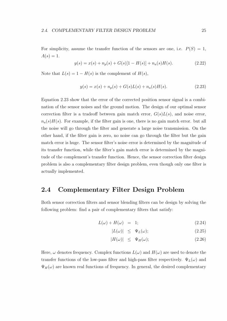
2.4. COMPLEMENTARY FILTER DESIGN PROBLEM 25
For simplicity, assume the transfer function of the sensors are one, i.e. P (S) = 1,
A(s) = 1.
y(s) = x(s) + np(s) + G(s)[1−H(s)] + na(s)H(s). (2.22)
Note that L(s) = 1−H(s) is the complement of H(s),
y(s) = x(s) + np(s) + G(s)L(s) + na(s)H(s). (2.23)
Equation 2.23 show that the error of the corrected position sensor signal is a combi-
nation of the sensor noises and the ground motion. The design of our optimal sensor
correction filter is a tradeoff between gain match error, G(s)L(s), and noise error,
na(s)H(s). For example, if the filter gain is one, there is no gain match error. but all
the noise will go through the filter and generate a large noise transmission. On the
other hand, if the filter gain is zero, no noise can go through the filter but the gain
match error is huge. The sensor filter’s noise error is determined by the magnitude of
its transfer function, while the filter’s gain match error is determined by the magni-
tude of the complement’s transfer function. Hence, the sensor correction filter design
problem is also a complementary filter design problem, even though only one filter is
actually implemented.
2.4 Complementary Filter Design Problem
Both sensor correction filters and sensor blending filters can be design by solving the
following problem: find a pair of complementary filters that satisfy:
L(ω) + H(ω) = 1; (2.24)
|L(ω)| ≤ ΨL(ω); (2.25)
|H(ω)| ≤ ΨH(ω); (2.26)
Here, ω denotes frequency. Complex functions L(ω) and H(ω) are used to denote the
transfer functions of the low-pass filter and high-pass filter respectively. ΨL(ω) and
ΨH(ω) are known real functions of frequency. In general, the desired complementary

26 CHAPTER 2. COMPLEMENTARY FILTERS
filters are designed by choosing appropriate values of ΨL(ω) and ΨH(ω) and then
solving the problem given by equations 2.24 through 2.26.
2.4.1 FIR Complementary Filter
For a finite impulse response (FIR) filter, the transfer function, Q(ω), is the Fourier
transform of its filter coefficients in the time domain, q(n):
Q(ω) = F(g(n)) =∑
n
q(n) cos(nω) + iq(n) sin(nω) (2.27)
The problem given by equations 2.24 through 2.26 becomes finding filter coeffi-
cients l(n) and h(n):
∑n
l(n) cos(nω) +∑
n
h(n) cos(nω) = 1; (2.28)
∑n
l(n) sin(nω) +∑
n
h(n) sin(nω) = 0; (2.29)
[(∑
n
l(n) cos(nω))2 + (∑
n
l(n) sin(nω))2]12 ≤ ΨL(ω); (2.30)
[(∑
n
h(n) cos(nω))2 + (∑
n
h(n) sin(nω))2]12 ≤ ΨH(ω); (2.31)
All variables in equation 2.28 through 2.31 are real numbers. Equations 2.28 and
2.29 are linear functions of variables h(n) and l(n). The left sides of 2.30 and 2.31
are quadrature functions of h(n) and l(n). Hence the problem defined by equations
2.28 through 2.31 is a convex optimization problem (specifically, a convex feasibility
problem)[11], which can be solved very efficiently [11].
Note that the convex feasibility problem defined by equations 2.28 through 2.31
is defined in continuous frequency. To solve the problem practically, the frequency
needs to be sampled. A set of frequency points ω1, ω2,...,ωi,...ωM need to be selected in
the frequency band of interest. For each frequency point, ωi, equations 2.28 through
2.31 have to be satisfied. Hence, the convex optimization problem has 2M equality
constraints and 2M inequality constraints. The method of selecting frequency samples
is discussed in the following sections.

2.4. COMPLEMENTARY FILTER DESIGN PROBLEM 27
ΨH(ω) and ΨL(ω) are the design parameters. In general, the design procedure is:
1. Select desired ΨH(ω) and ΨL(ω) based on practical needs, for example noise
levels of different sensors, gain error of different sensors, etc.
2. Solve the convex feasibility problem defined by equation 2.28 through 2.31.
3. If a solution is found, stop. Otherwise, relax constraints defined by ΨH(ω) and
ΨL(ω) and repeat step 2.
Because the globally optimized solutions can always be found for the above convex
optimization problem, the search for the feasible solution is complete. If there exists
an FIR filter pair h(n) and l(n) that satisfies the constraints defined by design param-
eter ΨH(ω) and ΨL(ω), the convex optimization solver id guarantees to generate the
solution of the problem, i.e. the filter coefficients. Otherwise, if there is no feasible
solution, the convex optimization solver generates a numerical proof that there is no
solution that meets the requirement.
A general linear time invariant complementary filter pair that satisfies equation
2.24 through 2.26 is called a absolute optimal filter pair. The absolute optimal filters
could be FIR or IIR filters. If the impulse response time and the sampling frequency
of the FIR filter are allowed to approach infinity, the solution of the problem defined
by equations 2.24 through 2.26 approaches the absolute optimal filter limit. Hence, if
there is enough calculation power to solve the convex problem defined by equations
2.28 through 2.31 for long enough FIR filters, the absolute optimal filters can be
approximated.
2.4.2 Simplification of the FIR Complementary Filter Design
Problem
To solve the FIR filter design problem of 2.28 through 2.31, it is simplified in the
following way.
Take the inverse Fourier transform of equation 2.24,
F−1(H(ω)) + F−1(L(ω)) = F−1(H(ω) + L(ω)) = F−1(1), (2.32)

28 CHAPTER 2. COMPLEMENTARY FILTERS
which gives
l(n) =
1− h(n) if n = 0;
−h(n) if n > 0.(2.33)
Hence l(n) can be eliminated and the optimization problem becomes: find h(n),
such that
[(1−∑
n
h(n) cos(nω))2 + (∑
n
h(n) sin(nω))2]12 ≤ ΨL(ω); (2.34)
[(∑
n
h(n) cos(nω))2 + (∑
n
h(n) sin(nω))2]12 ≤ ΨH(ω); (2.35)
Because ΨH(ω) and ΨL(ω) can be any arbitrary functions of ω, the design space
is huge. The advantage is that there is a lot of flexibility in the FIR filter design. The
disadvantage is that it is difficult to search through all possible design parameters in
the design space. Hence, it is helpful to search automatically for the best filter in the
design space. One can construct the convex optimization problem for variables h,ΨH
and ΨL:
minimize: V (h, ΨH , ΨL) (2.36)
such that: (2.37)
[(1−∑
n
h(n) cos(nω))2 + (∑
n
h(n) sin(nω))2]12 ≤ ΨL(ω); (2.38)
[(∑
n
h(n) cos(nω))2 + (∑
n
h(n) sin(nω))2]12 ≤ ΨH(ω); (2.39)
where, V (h, ΨH , ΨL) (called value function), is a convex function of h,ΨH and ΨL.
For example, one can chose
V =∑ωi
[ΨL(ωi)NL(ωi)]2 + [ΨL(ωi)NL(ωi)]
2. (2.40)
The convex optimization problem defined by this value function finds the optimal
filter that minimizes the total noise of the super sensor.

2.4. COMPLEMENTARY FILTER DESIGN PROBLEM 29
2.4.3 Example of FIR Complementary Filter Design Using
SeDuMi
Design Requirement
In our vibration isolation system, we need a high pass sensor correction filter that
has the following properties:
1. Form 0 to 0.008 Hz, the magnitude of the filter’s transfer function should be
less than or equal to 8× 10⁻⁴. We chose to have a ”flat” magnitude at very low
frequencies to avoid numerical problems which will be discussed later in this
section.
2. From 0.008 Hz to 0.04 Hz, it attenuates the input signal proportional to fre-
quency cubed. Because the noise level of the horizontal inertial sensor increases
very rapidly (proportional to inverse frequency cubed) at low frequencies, we
need a powerful high pass filter to get rid of the sensor noise;
3. Between 0.04 Hz and 0.1 Hz, the magnitude of the transfer function should be
less than 3. Because the inertial sensor’s noise level is low in this frequency
band, the filter is allowed to magnify the sensor noise here;
4. Above 0.1 Hz, the maximum of the magnitude of the complement filter should
be as close to zero as possible. As mentioned above, the magnitude of the
complementary filter determines the amount of gain match error in the sensor
correction system. In our system, we would like to have the magnitude of
the complementary filter to be less than 0.1. However, to make this problem
an optimization problem, rather than a feasibility problem, we construct this
problem to automatically search for the best filter that satisfies constraints 1
through 3. If the optimal filter solution does not satisfy the design requirement,
i.e. complementary filter’s magnitude less than 0.1, it implies that that there
does not exist a FIR filter that satisfies all of our design requirements, and the
constraints of 1 through 3 need to be loosened. Through this approach, we can

30 CHAPTER 2. COMPLEMENTARY FILTERS
tradeoff between the gain match error and the sensor noise error as indicated
by equation 2.23.
Frequency Sampling
The sensor correction filter is designed to have a sampling frequency of 1.67 Hz
(sample time is 0.6 second). The length of the filter is 512. How to chose sampling
frequencies and filter length will be discussed in later sections. Let us just assume
that they are fixed numbers now.
The impulse response of the filter is about 300 second long, which implies the
frequency discrimination of this filter is about 0.003 Hz. Hence, in general, the gap
between the neighboring frequency samples should be less than 0.003 Hz such that the
sampled frequency response can represent the actual transfer function of the filter. On
the other hand, the number of frequency samples determines the number of constraints
in the convex optimization problem. If there are too many frequency samples, the
amount of calculations required to solve the problem becomes impractical.
The filter’s transfer function changes dramatically at low frequencies. For example,
at 0.008 Hz the upper limit of the magnitude of the transfer function is 8×10⁻⁴, but at
0.0016 Hz it becomes 6.4× 10⁻³. Hence, more samples are needed at low frequencies
than at high frequencies. For frequencies below 0.04 Hz, the frequency sample rate
is 4.06 × 10⁻⁴ Hz per sample. For frequencies above 0.04 Hz, the frequency sample
rate is 8.12 × 10⁻⁴ Hz. The fast changing transfer function at low frequencies can
also cause numerical problems for the convex optimization solver program. To avoid
those problems, the upper limit of the magnitude of the filters transfer function were
kept flat as indicated by the constraint 1.
Quadratic Cone Programming and SeDuMi
A quadratic cone is by defined as
Qcone := (x1, x2) ∈ < × <(N−1)| x1 ≥ ‖x2‖ (2.41)

2.4. COMPLEMENTARY FILTER DESIGN PROBLEM 31
where ‖ · ‖ denotes the Euclidean norm.
‖x‖ = (∑
i
x2i )
1/2. (2.42)
The quadratic cone is also known as the second order cone or Lorentz cone.
The quadratic cone programming optimization problem is:
minimize: cT x (2.43)
such that: Ax = b, x ∈ Qcone. (2.44)
Its dual problem is:
maximize: bT y (2.45)
such that: c− AT y ∈ Qcone. (2.46)
SeDuMi [48] solves quadratic cone programming and its dual problem at the same
time, i.e., given vector c, b and matrix A, it generates solution x and y at the same
time.
We format our FIR filter design problem to the dual problem. The magnitude
constraints can be easily converted into quadratic cone constraints in the format
as equation 2.46. For example, inequality constraint 2.31 at frequency ω can be
formatted as:
‖[νc(ω); νs(ω)]h‖ ≤ ΦH(ω) (2.47)
where
h = [h(0), h(1), ..., h(N − 1)]T (2.48)
νc = [1, cos(ω), ..., cos((N − 1)ω)] (2.49)
νs = [0, sin(ω), ..., sin((N − 1)ω)] (2.50)

32 CHAPTER 2. COMPLEMENTARY FILTERS
Construct
c = [ΦH(ω), 0, ..., 0]T (2.51)
AT = [0, ... ,0; νc(ω); νs(ω)] (2.52)
and we have
c− AT y ∈ Qcone. (2.53)
The other constraints can be formatted into Qcone format in similar ways. To convert
the convex feasibility problem to a convex optimization problem, introduce a new
variable, t, as the maximum gain match error above 0.1 Hz, i.e. the maximum
magnitude of ΦL. The FIR filter design problem is formatted as:
for variable vector y = [t, h(1), h(2) ,..., h(N − 1)]T (2.54)
maximize: − t = [ -1 0 0 ... 0]T y (2.55)
such that:
for constants ω = 0, 4.06× 10⁻⁴, ... , 0.008 Hz :
‖[0 νc(ω); 0 νs(ω)]y‖ ≤ 8× 10⁻⁴; (2.56)
for constants ω = 0.008, 0.008 + 4.06× 10⁻⁴, ... , 0.04 Hz :
‖[0 νc(ω); 0 νs(ω)]y‖ ≤ 8× ω3; (2.57)
for constants ω = 0.04, 0.04 + 8.12× 10⁻⁴, ... , 0.1 Hz :
‖[0 νc(ω); 0 νs(ω)]y‖ ≤ 3; (2.58)
for constants ω = 0.1, 0.1 + 8.12× 10⁻⁴, ... , 0.83 Hz :
‖[1 0]T − [0 νc(ω); 0 νs(ω)]y‖ ≤ t (2.59)
Note that when these formulas are applied, the unit of frequency, ω, needs to be
converted to radians:
ω (rad) =ω (Hz)
sample frequency (Hz). (2.60)

2.4. COMPLEMENTARY FILTER DESIGN PROBLEM 33
Results
Totally, there are 513 variables and about 1500 constraints in this convex optimization
problem. It takes about 10 minutes for a PC with 1 gigabyte of memory and one
Pentium 4 CPU to solve the problem.
Figure 2.7 shows the transfer functions of the FIR complementary filter pair.
The high pass filter satisfies all the magnitude constraints at low frequencies. Its
complement, the low pass filter, shows that the gain match error is about 0.05 above
0.1 Hz.
Figure 2.6 shows the time domain impulse response of the high pass filter. It looks
like the impulse response of a damped oscillator. The oscillation period is about 0.04
Hz to 0.1 Hz, where the transfer function of the filter in the frequency domain has a
large overshoot.
−50 0 50 100 150 200 250 300 350−0.5
0
0.5
1
time (second)
highpass
−50 0 50 100 150 200 250 300 350−0.5
0
0.5
1
time (second)
lowpass
Figure 2.6: Time domain impulse response of the FIR complementary filter pair
designed using SeDuMi convex optimization tool.
The Effect of Filter Length and Sampling Frequency of the FIR Filters
The impulse response time of an FIR filter is given by its sample time ts and its filter
length (number of filter coefficients) N .
T = Nts. (2.61)

34 CHAPTER 2. COMPLEMENTARY FILTERS
10−3
10−2
10−1
100
10−3
10−2
10−1
100
101
mag
nitu
de (
m/m
)
highpasslowpass
10−3
10−2
10−1
100
−200
−100
0
100
200
freq (Hz)
phas
e (d
egre
e)
Figure 2.7: Transfer functions of a pair of FIR complementary filters designed usingSeDuMi convex optimization tool.

2.4. COMPLEMENTARY FILTER DESIGN PROBLEM 35
The impulse response time determines its frequency resolution: δf .
δf =1
T. (2.62)
The filters with longer impulse response have better performance, but on the other
hand, they requires more calculation to design and to implement. The effect of filter
length and sample time on complementary FIR filter performance is studied in this
section.
A set of FIR complementary filters are designed with different filter length. All the
other design parameters for those filters were kept the same as the previous example.
The transfer functions of the complementary filters are shown in figure 2.8. Their
time domain impulse responses of the low pass filters of the complementery filter
pairs are shown in figure 2.9. In general, filters with more coefficients have better
performance, which is measured by the gain match error (magnitude of the low pass
filter above 0.1 Hz). Because the sample frequencies were kept the same (at 1.67 Hz),
for all these filters, filters with more coefficients have a longer impulse response time,
which implies better frequency resolution. As shown in figure 2.8, the filter with 1024
coefficients has much sharper transfer function than the filter with 64 coefficients
has. Because the filters with sharper transfer function can make a better use of the
frequency band of 0.04 Hz to 0.1 Hz, where overshoot is allowed, they tends to have
less gain match error above 0.1 Hz. However, as shown in figure 2.10, when filter
length is longer than a certain level, its significance becomes much less. For example,
the gain match error of filter with 1024 coefficients is only 5% better than that of the
filter with 512 coefficients. This implies that the optimal FIR filter is approaching the
absolute optimal filter and that the absolute optimal filter’s impulse response after
1024 second is close to zero. In the time domain, all the filters have a similar response
in the first several seconds. Another similarity is that all the filter’s time response is
close to zero at the end. One intuitive explanation of this phenomenon is that the
optimization solver tried to avoid a sudden turnoff of the filter’s impulse response,
because it will cause bad frequency domain behavior. The peak to peak value of the
impulse response of the 1024 coefficient filter in the last 200 seconds is less than 2%

36 CHAPTER 2. COMPLEMENTARY FILTERS
of the max peak to peak value, which is also an indication that the optimal FIR filter
is approaching the absolute optimal filter.
Another way to change the impulse response time is to change the sample time.
The effect of sample time is similar to that of the filter length. The set of transfer
functions of the complementary FIR filters are shown in figure 2.11. The time domain
impulse response of the low pass filters are shown in figure 2.12. These set of FIR
filters with different sample times have the same values of impulse response time as
the set of FIR filters with different filter length. Figure 2.13 compares the gain match
errors of these two set of filters. The effect of the sample time and filter length are
similar, but there are till some realizable difference. For example, the filter with 1024
coefficients and sample time of 0.6 seconds and the filter with 512 coefficients and
sample time of 1.2 seconds has the sample impulse response time, but the latter has
less gain match error. The reason for this difference can be explained by the frequency
domain transfer function. In figure 2.11, the transfer function of the filter with 1.2
second sample time has a peak around 0.83 Hz. Because the sampling frequency of
this filter is at 0.83 Hz, the peak comes from the reflection of the filter’s transfer
function below 0.41 Hz. On the other hand, the transfer function of the filter with
1024 coefficient in figure 2.8 does not have such a peak. Hence, the filter with longer
sample time achieves better performance in the range of 0.1 to 0.85 Hz, but the at
cost of worse performance at 0.86 Hz. The same theory can be used to explained
the other gain error difference between these two different sets of filters. Details of
tradeoff between gain match error and the frequency reflection peak will be discussed
in the next chapter.
Tradeoff Between Gain Match Error and Overshoot
The convex optimization FIR filter design method can also be used to study the
engineering tradeoff between different design parameters. Figure 2.14 shows transfer
functions of a set of complementary filters with different magnitude constraint on the
highpass filter between 0.04 Hz and 0.1 Hz (also called overshoot). Figure 2.15 shows
the relationship between overshoot and gain match error. One can realize that when
overshoot is more than 3, its contribution in minimizing the gain match error is not

2.4. COMPLEMENTARY FILTER DESIGN PROBLEM 37
10−2
10−1
100
10−2
10−1
100
101
mag
nitu
de (
m/m
)
freq (Hz)10
−210
−110
0
10−2
10−1
100
101
freq (Hz)
len = 64len = 128len = 256len = 512len = 1024
10−1
100
mag
nitu
de (
m/m
)
freq (Hz)
high pass
10−1
100
freq (Hz)
low pass
Figure 2.8: Optimal FIR complementary filters for different filter lengths. The detailsof the transfer function between 0.03 Hz and 0.12 Hz are shown in the lower plots.

38 CHAPTER 2. COMPLEMENTARY FILTERS
0 200 400 600−0.2
0
0.2len = 64
0 200 400 600−0.2
0
0.2len = 128
0 200 400 600−0.2
0
0.2len = 256
0 200 400 600−0.2
0
0.2len = 512
0 200 400 600−0.2
0
0.2
time (second)
len = 1024
Figure 2.9: Time domain impulse response of the lowpass optimal FIR filters in thecomplementary filter pairs with different filter length.

2.4. COMPLEMENTARY FILTER DESIGN PROBLEM 39
64128 256 512 10240.04
0.05
0.06
0.07
0.08
0.09
0.1
time (second)
mat
ch e
rror
Figure 2.10: Gain match errors (magnitudes of the lowpass filters above 0.1 Hz) asa function of filter length. It seems that after the filter length is longer than somethreshold, increasing the filter length does not reduce the gain match error any more.
very significant. For this reason, an overshoot of 3 was chosen for the previous filter.
Changing the Shape of the Gain Match Error
In previous sections the magnitude of the low pass filter above 0.1 Hz is almost
constant because the constraint of equation 2.59 is constant with respect to frequency.
Filters with different gain error shape can be designed by introducing a shape function
to the constrain:
‖[1 0]T − [0 νc(ω); 0 νs(ω)]y‖ ≤ W (ω)t (2.63)
For example let W (ω) = ω−1, we can design a filter whose gain match error decreases
as the inverse of the frequency. The transfer function of the designed complementary
filter pair is shown in figure 2.16

40 CHAPTER 2. COMPLEMENTARY FILTERS
10−2
10−1
100
10−2
10−1
100
101
mag
nitu
de (
m/m
)
freq (Hz)10
−210
−110
0
10−2
10−1
100
101
freq (Hz)
sample time = 0.07 secsample time = 0.15 secsample time = 0.30 secsample time = 0.60 secsample time = 1.20 sec
10−1
100
mag
nitu
de (
m/m
)
freq (Hz)
high pass
10−1
100
freq (Hz)
low pass
Figure 2.11: Optimal FIR complementary filters for different filter lengths. Thedetails of the transfer function between 0.03 Hz and 0.12 Hz are shown in the lowerplots.
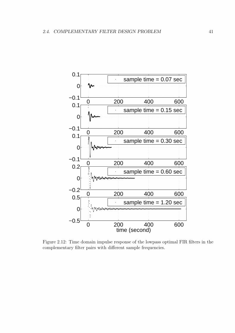
2.4. COMPLEMENTARY FILTER DESIGN PROBLEM 41
0 200 400 600−0.1
0
0.1sample time = 0.07 sec
0 200 400 600−0.1
0
0.1sample time = 0.15 sec
0 200 400 600−0.1
0
0.1sample time = 0.30 sec
0 200 400 600−0.2
0
0.2sample time = 0.60 sec
0 200 400 600−0.5
0
0.5
time (second)
sample time = 1.20 sec
Figure 2.12: Time domain impulse response of the lowpass optimal FIR filters in thecomplementary filter pairs with different sample frequencies.

42 CHAPTER 2. COMPLEMENTARY FILTERS
0 100 200 300 400 500 600 7000.04
0.05
0.06
0.07
0.08
0.09
0.1
impulse response time (second)
mat
ch e
rror
change filter lenchange sample time
Figure 2.13: Gain match errors (magnitudes of the lowpass filters above 0.1 Hz) as afunction of sample time.
10−2
10−1
100
10−2
10−1
100
101
mag
nitu
de (
m/m
)
freq (Hz)10
−210
−110
0
10−2
10−1
100
101
freq (Hz)
overshot = 1overshot = 2overshot = 3overshot = 4overshot = 5
Figure 2.14: The maximum gain match errors (magnitudes of the lowpass filters above0.1 Hz) as a function of sample time.

2.5. IIR COMPLEMENTARY FILTERS 43
1 2 3 4 50
0.05
0.1
0.15
0.2
0.25
0.3
0.35
overshot
mat
ch e
rror
Figure 2.15: Gain match errors (magnitudes of the lowpass filters above 0.1 Hz) as afunction of sample time.
2.5 IIR Complementary Filters
For an infinite impulse response (IIR) filter, the transfer function, K(ω), can also be
easily obtained from its time domain numerator coefficients kN(n) and denominator
coefficients kD(n):
K(ω) =
∑kN(n)e−inω
∑kD(n)e−inω
. (2.64)
However, finding kN(n) and kD(n) that satisfy equations 2.24 through 2.26 is not a
convex problem, and hence very difficult to solve.
For the most of the IIR complementary filters used in this thesis, they are designed
using the following procedure:
1. Design a pair of desired highpass and lowpass filter.
2. Check to make sure that the sum of these two filters is invertible.
3. Normalize the two filters such that they are complementary.
For example, the filter shown at the beginning of this chapter in figure 2.1 is

44 CHAPTER 2. COMPLEMENTARY FILTERS
10−3
10−2
10−1
100
101
10−3
10−2
10−1
100
101
mag
nitu
de (
m/m
)
highpasslowpass
10−3
10−2
10−1
100
101
−200
−100
0
100
200
freq (Hz)
phas
e (d
egre
e)
Figure 2.16: Complementary filter with the gain match error (magnitude of the lowpass filter at high frequencies) decreases as the inverse of the frequency.

2.6. SUMMARY 45
designed by normalizing the highpass filter and the lowpass filter shown in figure
2.17. The transfer function of the sum does not have overall phase lag, so it is
invertible.
2.6 Summary
Because the IIR complementary filters can only be designed by trial and error, their
performance is not as good as the optimal FIR filters. Figure 2.18 shows the difference
of the optimal FIR filters and a typical IIR filter designed using the above procedure.
The FIR filter and the IIR filter have similar overshoot and gain match error (at 0.16
Hz), but the FIR filters have much better low frequency performance.
The difference between FIR and IIR complementary filters is summarized in table
2.1.
FIR IIRdesign convex, easy non-convex, difficult
implementation complex simplecomputation much littleperformance great ok
Table 2.1: Comparing FIR and IIR complementary filters.

46 CHAPTER 2. COMPLEMENTARY FILTERS
10−2
10−1
100
101
102
10−3
10−2
10−1
100
101
102
mag
nitu
de (
m/m
)
highpasslowpasssum
10−2
10−1
100
101
102
−400
−300
−200
−100
0
100
freq (Hz)
phas
e (d
egre
e)
Figure 2.17: Complementary IIR filters can be constructed by normalizing a pair ofIIR filters. The transfer function of the sum does not have overall phase lag, so it isinvertible.

2.6. SUMMARY 47
10−3
10−2
10−1
100
10−3
10−2
10−1
100
101
102
mag
nitu
de (
m/m
)FIR highpassFIR lowpassIIR highpassIIR lowpass
10−3
10−2
10−1
100
−200
−100
0
100
200
freq (Hz)
phas
e (d
egre
e)
Figure 2.18: Compare the performance of FIR and IIR filter. The FIR filter andthe IIR filter have similar overshoot and gain match error (at 0.16 Hz), but the lowfrequency performance is very different. The sharp noise reduction of the FIR filtersis essential for the low frequency isolation systems.

48 CHAPTER 2. COMPLEMENTARY FILTERS

Chapter 3
Polyphase FIR Filter
Implementation
3.1 Introduction
In chapter 2, it is shown that FIR complementary filters have superior performance
than the IIR filters. However, the amount of calculations required to implement the
FIR filters is too large to be practical if they are implemented in the traditional way
with today’s computer technology.
In a standard FIR filter with filter coefficients q, at each time step, the output, y,
is calculated from the input, x, by
y(n) =N−1∑m=0
q(m)x(n−m). (3.1)
So, at each time step, 2N(N multiplications and N additions) FLoating Point Op-
erations(FLOPs) need to be calculated. Hence, the number of FLOPs per second
(FLOPs/sec) for a FIR filter with sampling frequency fs is
N = 2Nfs. (3.2)
From chapter 2, it is known that to obtain a sharp transition between a stop-band
49

50 CHAPTER 3. POLYPHASE FIR FILTER IMPLEMENTATION
and pass-band for FIR filters, the filter has to have high frequency resolution, which
is determined by the filters impulse response time T . Since
T =N
fs
, (3.3)
we have
N = 2Tf 2s . (3.4)
In our vibration isolation system prototype, the sampling frequency of the digital
control system is at 2500 Hz. If a FIR filter with 300 second impulse response time is
implemented directly, the required FLOPS is 3.75×10⁹ operations per second, which
is too large for most processors today.
3.2 Down Sampling
To reduce the FLOPs/sec for FIR filters, the sampling frequency of the low pass FIR
filters can be reduced by down sampling as shown in figure 3.1. The down sampling
block with down sampling ratio of D just select one data sample from every D data
samples from the incoming data stream and send it to its output and throws the rest
of the data points away. The up sampling block does the opposite, it interpolates
zeros inbetween the input data points and then sends them to output. [54].
A low pass anti-aliasing filter is used before the down sampling to reduce the
amount of high frequency signals aliased to the low frequencies when the signal is
down sampled. Similarly another low pass interpolation filter is used to avoid the
low frequency signal from aliasing to the high frequencies. The introduction of the
anti-aliasing filter and the interpolation filter has two effects on the FIR filter. First,
they reduce the aliasing noise of the filter. Second, they contribute to the overall
transfer function of the whole filter. Figure 3.2 shows a low pass filter with cutoff
frequency of 0.5 Hz. In the following examples in this section, this filter is used as
both the anti-aliasing filter and the interpolation filter in a down sampling FIR filter
system with the original FIR filter shown in figure 2.7.

3.2. DOWN SAMPLING 51
Figure 3.1: To reduce the number of floating point calculation per second (FLOPS)
by reducing the sampling frequency of the FIR filter. An anti-aliasing filter is used
before down sampling to reduce the amount of high frequency signals aliased to the
low frequencies when the signal is down sampled. Similarly an interpolation filter is
used to avoid low frequency signal to alias to high frequencies.
10−3
10−2
10−1
100
10110
−4
10−3
10−2
10−1
100
101
freq (Hz)
mag
nitu
de (
m/m
)
Figure 3.2: Low pass filters with cutoff frequency of 0.5 Hz, as an example of the
anti-aliasing filter or interpolation filter in figure 3.1.
Let D denote the down sampling ratio between the sampling frequency of the
outside digital system fs0 and the sampling frequency of the FIR filter fs. Suppose
the input signal (in the frequency domain) is x(f), the aliasing noise due to down
sampling of the signal before entering the FIR filter between zero frequency and fs/2

52 CHAPTER 3. POLYPHASE FIR FILTER IMPLEMENTATION
is
xDn(f) =D∑
d=1
x(dfs − f)A(dfs − f), (3.5)
where A(·) denotes the frequency response of the anti-aliasing filter. If the amplitude
spectral density (ASD) of the input signal is assumed to be 1 m/√
Hz, and the low
pass filter shown in figure 3.2 is used as the anti-aliasing filter, the ASD of different
aliasing components are shown in figure 3.3. Because A(s) is a low pass filter, the
first term in the summation of equation 3.5 dominates the down sampling noise. To
reduce the down sampling noise, we need to increase the sampling frequency of the
FIR filter or to decrease the cutoff frequency of the anti-aliasing filter.
10−2
10−1
10010
−4
10−2
100
102
freq (Hz)
AS
D (
m/r
tHz)
fs
Original signal1st order image2nd order image3rd order image
Figure 3.3: Signal aliasing due to down sampling. The signal coming out of the
anti-aliasing filter is shown as the original signal. The sampling frequency of the FIR
filter, fs, is 1.67 Hz. The high order aliasing components contributes to the down
sampled signal between zero and fs/2. The down sampling aliasing noise is about 1%
in this plot.
Similarly, up sampling aliasing noise is introduced to the signal when the output
of the FIR filter is interpolated to match the sampling frequency of the outside digital
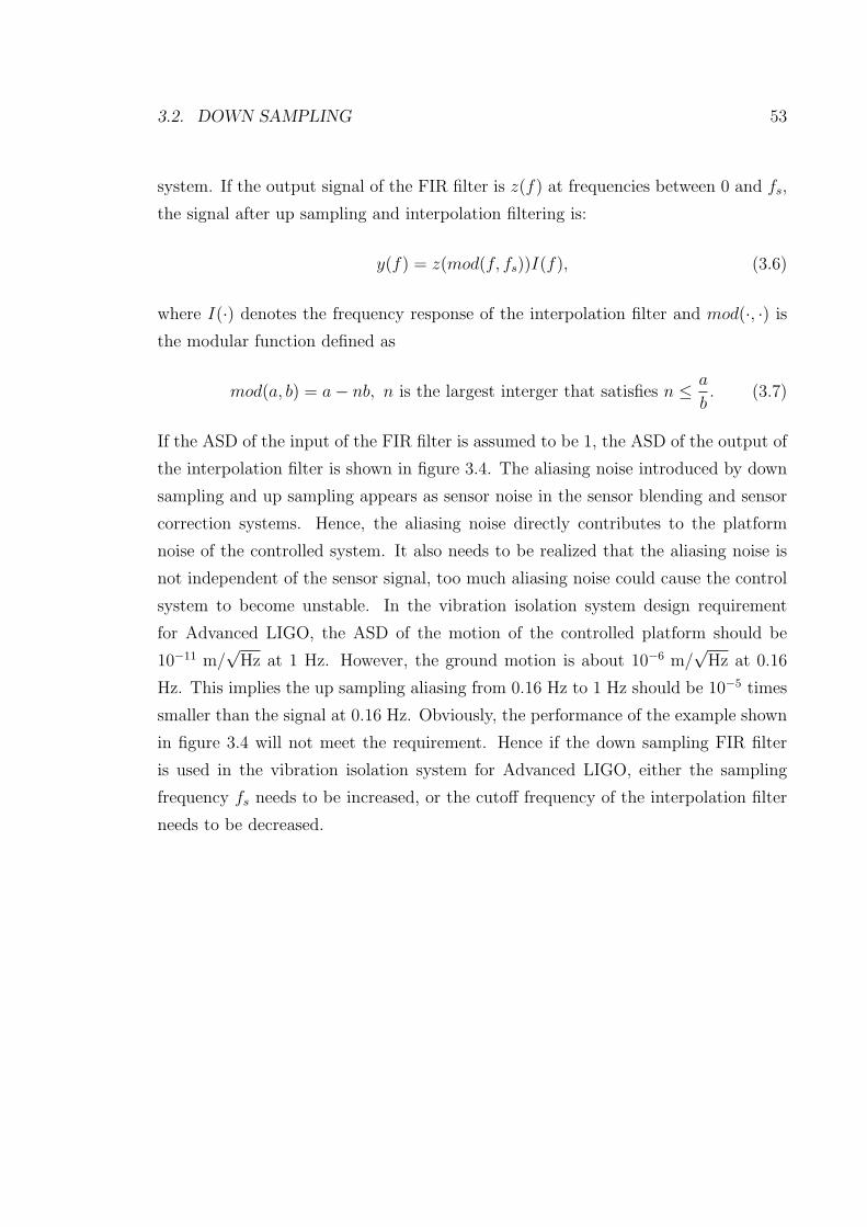
3.2. DOWN SAMPLING 53
system. If the output signal of the FIR filter is z(f) at frequencies between 0 and fs,
the signal after up sampling and interpolation filtering is:
y(f) = z(mod(f, fs))I(f), (3.6)
where I(·) denotes the frequency response of the interpolation filter and mod(·, ·) is
the modular function defined as
mod(a, b) = a− nb, n is the largest interger that satisfies n ≤ a
b. (3.7)
If the ASD of the input of the FIR filter is assumed to be 1, the ASD of the output of
the interpolation filter is shown in figure 3.4. The aliasing noise introduced by down
sampling and up sampling appears as sensor noise in the sensor blending and sensor
correction systems. Hence, the aliasing noise directly contributes to the platform
noise of the controlled system. It also needs to be realized that the aliasing noise is
not independent of the sensor signal, too much aliasing noise could cause the control
system to become unstable. In the vibration isolation system design requirement
for Advanced LIGO, the ASD of the motion of the controlled platform should be
10−11 m/√
Hz at 1 Hz. However, the ground motion is about 10−6 m/√
Hz at 0.16
Hz. This implies the up sampling aliasing from 0.16 Hz to 1 Hz should be 10−5 times
smaller than the signal at 0.16 Hz. Obviously, the performance of the example shown
in figure 3.4 will not meet the requirement. Hence if the down sampling FIR filter
is used in the vibration isolation system for Advanced LIGO, either the sampling
frequency fs needs to be increased, or the cutoff frequency of the interpolation filter
needs to be decreased.

54 CHAPTER 3. POLYPHASE FIR FILTER IMPLEMENTATION
10−3
10−2
10−1
100
10110
−5
10−4
10−3
10−2
10−1
100
101
freq (Hz)
m/r
tHz
Figure 3.4: Signal aliasing due to up sampling.
At frequencies between 0 to fs, the anti-aliasing filter and the interpolation filter
contribute to the transfer function of the overall down sampling FIR filter system,
which could degrade the performance of the overall FIR filter. For example, the
transfer functions of a down sampling FIR complementary filter pair is shown in figure
3.5. The gain match error of the overall high pass filter is about 9 times larger than
that of the original filter at 0.3 Hz. If this filter is used as the sensor correction filter,
the isolation performance will not meet LIGO’s requirement. To address the problem
for down sampling FIR filters, we need to increase either the sampling frequency of
the FIR filter or the cutoff frequencies of the anti-aliasing filter and the interpolation
filter.

3.2. DOWN SAMPLING 55
10−3
10−2
10−1
10010
−3
10−2
10−1
100
101
102
freq (Hz)
mag
nitu
de (
m/m
)
overall low passoverall high passoriginal FIR low passanti−aliasing and interpolation
Figure 3.5: The anti-aliasing filter and interpolation filter contributes to the transfer
function of overall down sampling FIR filter system. As result, the gain match error
of the overall high pass filter is about 9 times larger than that of the original filter at
0.3 Hz.
In conclusion, in a down sampling FIR filter system, if the sampling frequency
of the FIR filter is fixed, the cutoff frequencies of the anti-aliasing filter and the
interpolation filter determines the tradeoff between signal aliasing noise and transfer
function error. In our examples in this section, these two problems can not be solved
at the same time unless the sampling frequency is dramatically increased. However,
increasing the sampling frequency will cause two other problems. First, the run time
FLOPS will increase proportional to f 2s . Second, the number of coefficients in the FIR
filter will increase proportional to fs, which will cause the FLOP used to solve the
FIR filter design problem to increase proportional to f 3s . Either of the these problems
could make the design impractical.

56 CHAPTER 3. POLYPHASE FIR FILTER IMPLEMENTATION
3.3 Polyphase FIR Filter Implementation
A technique called polyphase FIR filtering, as shown in Figure 3.9, is designed to
reduce the the calculation load of traditional down sampling FIR filters. The incoming
data stream is divided into m sub-streams by a cyclic distributer according to the
data samples’ arrival time. Hence, each sub-stream has the sample rate of fs/m (in
Figure 3.9, m = 3). The FIR filters on each sub-stream are identical traditional FIR
filters which work at frequency ff = fs/m. At each time step, the cyclic collector
picks up an output sample from the FIR filter that is working in that phase and sends
it to the output. Hence, the output sample rate is fs, which is the same as the input
sample rate.
FIR
FIR
FIR
In Out
Cyclic
DistributorCyclic
Collector
012 1 10
00
2 2
012
Figure 3.6: Polyphase FIR filter implementation. The three FIR filters have identical
filter coefficients and each operates at frequency ff , but are offset in phase. The cyclic
distributor distributes the incoming data samples to different FIR filters according
to the samples’ arriving time phase. At each time step, the cyclic collector picks up
an output sample from the FIR filter with the appropriate phase and sends it to the
output. Hence, the overall sampling frequency is fs = m · ff , where m is the number
of cyclic phases.

3.4. TRANSFER FUNCTION COMPENSATION 57
The total amount of calculation that is required by the polyphase FIR filter is
given by the total of m parallel FIR filters:
Np = 2mTff2 = 2Tfsff = 2
Nm
, (3.8)
which is m times smaller than what the traditional FIR filter requires.
This polyphase FIR filter is used to replace the FIR filter in the down sampling
system shown in figure 3.1. The down sampling polyphase FIR filter is shown in
figure 3.7. Because the signal sampling frequency is allowed to be higher than the
filter sampling frequency in polyphase filters, the anti-aliasing and interpolation filter
design becomes easier. As shown in figure 3.8, the signal sampling frequency is at
50 Hz and the signal below 1 Hz only aliases to frequencies above 50 Hz as shown in
figure 3.3.
Figure 3.7: Polyphase FIR filter with down sampling.
3.4 Transfer Function Compensation
The output of the polyphase FIR filter is given by
y(n) =
Nf−1∑q=0
x(n− qm)f(q), (3.9)
where x(n) denotes the nth input signal, y(n) denotes the nth output signal, Nf is
the number of coefficients of each FIR filter and f(q) denotes the qth filter coefficient
of the FIR filter.
If the transfer function of each FIR filter is f(ω), ω ∈ [0, ff ], the transfer function

58 CHAPTER 3. POLYPHASE FIR FILTER IMPLEMENTATION
10−2
100
10210
−4
10−2
100
102
freq (Hz)
mag
nitu
de (
m/m
)
Figure 3.8: Interpolation filter for polyphase down sampling FIR filter.
of the polyphase FIR filter is given by:
P (ω) = f(mod(ω, ff )), ω ∈ [0, fs]. (3.10)
At low frequencies, when ω ∈ [0, ff ], P (ω) is exactly the same as F (ω). However,
is obvious that P (ω) is not perfect at higher frequencies. In fact, P (ω) is a periodic
repetition of the function of F (ω) with a frequency period of ff . An example of the
transfer function of a polyphase FIR filter is shown in figure 3.9.

3.4. TRANSFER FUNCTION COMPENSATION 59
10−4
10−2
100
10210
−2
10−1
100
101
freq (Hz)
mag
nitu
de (
m/m
)
Figure 3.9: Transfer function of the high pass polyphase FIR filter based on the high-
pass FIR filter shown in Figure 2.7. The sampling frequency of the FIR filter, fs, is
1.67 Hz. The the peaks at around fs, 2fs, 3fs and so on are the frequency reflection
of the low frequency component below 0.1 Hz.
Additional filters could be used to compensate the non-ideal transfer function of
the polyphase FIR filter at frequencies above the filter sample frequency. First, a
low pass IIR filter, La, as shown in figure 3.10(a), can be used to compensate the
high frequency transfer function of a low pass polyphase FIR filter. The high pass
complement can be simply implemented as in figure 3.10(b). After the compensation,
the transfer function of the overall complementary filter pair (Lcp, Hcp) becomes:
Lcp(ω) = Lp(ω)La(ω) (3.11)
Hcp(ω) = 1− Lcp(ω) (3.12)
= 1− (1−Hp(ω))(1−Ha(ω)) (3.13)
= Hp(ω)− Lp(ω)Ha(ω), (3.14)
where the Ha denotes the complement of La. Equation 3.11 and 3.14 show that the
compensation filter design problem is also a complementary filter design problem:

60 CHAPTER 3. POLYPHASE FIR FILTER IMPLEMENTATION
|La| is preferred to be low at high frequencies such that the high frequency peaks of
Lp is attenuated; |Ha| is prefer to be low at low frequencies. In general, one would
like to have
|Lcp| ≤ ΨLc (3.15)
|Hcp| ≤ ΨHc, (3.16)
where ΨLc and ΨHc are magnitude constrains for the overall complementary filters. If
La and Ha are FIR filters, equation 3.16 and 3.15 defines an other convex optimization
problem for fixed Lp and Hp. Practically, one can design the compensation filters
which satisfies
|Lp(ω)Ha(ω)| ¿ |Hp(ω)| (3.17)
(3.18)
, such that Hp dominates the overall transfer function Hcp. For example,
|Lp(ω)Ha(ω)| ≤ 0.2|Hp(ω)|. (3.19)
The frequency resolution of the compensation filters do not need to be as high as the
original FIR filters. Hence, simple IIR filters can meet the requirement. It worth
mentioning that it is easier to compensate the low pass FIR filter than to compensate
the high pass FIR filter using a low pass IIR filter because we do not care about the
phase of the low pass filter at high frequencies. To further simply the structure of
the whole filter, the compensation low pass filter can also be used as the anti-aliasing
filter.
Similarly, a high pass filter can be used to compensate the transfer function of the
high pass polyphase FIR filter. In the original FIR filter design, the magnitude of the
transfer function of the high pass filter is flat below 0.008 Hz because the FIR filter
has not enough frequency resolution below that frequency. A high pass filter Hb can
be applied to make the magnitude of the transfer function continue to decrease as a
function proportional to frequency cubed below 0.008 Hz as shown in figure . The

3.4. TRANSFER FUNCTION COMPENSATION 61
final implementation of the complementary filter pair is shown in figure 3.12 (c) and
(d).
10−4
10−3
10−2
10−1
100
101
10210
−4
10−3
10−2
10−1
100
101
102
freq (Hz)
mag
nitu
de (
m/m
)L
cpH
cpL
a1−L
a
Figure 3.10: Low pass IIR filter La for compensating the high frequency transfer
function of a low pass FIR polyphase filter in a complementary filter pair.
10−4
10−3
10−2
10−1
100
101
10210
−4
10−3
10−2
10−1
100
101
102
freq (Hz)
mag
nitu
de (
m/m
)
final low passfinal high pass1−H
bH
b
Figure 3.11: High pass IIR filter Hb for compensating the low frequency transfer

62 CHAPTER 3. POLYPHASE FIR FILTER IMPLEMENTATION
function of the high pass FIR polyphase filter in a complementary filter pair. At low
frequencies, the final transfer function of the high pass filter is no longer flat.
Figure 3.12: Transfer function compensation of polyphase FIR filter. (a) A low pass
filter La is used with the low pass FIR filter to attenuate its peaks at high frequencies.
(b) The high pass filter is simply built as the complement of (a). (c) A high pass
filter is use to compensate the low frequency transfer function of (b). (d) The final
low pass filter is implemented as the complement of the high pass filter in (c)

3.5. SUMMARY 63
3.5 Summary
The polyphase FIR filter 1 decouples the noise problem and the transfer function
problem in a FIR filter design by allowing different filter sampling frequency and
signal sample frequency. Practically ff could be much smaller than fs, which saves a
lot of calculation operations.
The transfer function design of the polyphase FIR complementary is separated
into three frequency bands:
1. In the transition band, where the high pass filter and the low pass filter have
comparable magnitude, there are a lot of structures in the transfer functions
which requires high frequency resolution to implement. Hence, a lot of design
effort and run time calculation capability is used to build the FIR complemen-
tary filter pair which dominates the whole transfer function in this frequency
band.
2. At high frequencies, there is not much structure in the transfer functions: all
we need to do is to allow the high pass filter to pass and the low pass filter
to stop. Hence, it make sense to use simple (both simple to design and simple
to implement) IIR filter, such as La, to dominate the transfer function in this
band. Of course, it is possible to use another FIR filter to replace the IIR filter
for even better performance.
3. Similarly at low frequencies, a simple IIR filter Hb is used to dominate the
transfer functions.
Similar FIR filter structures, called multi-phase FIR filters, are widely used in
digital signal processing systems [54]. There are two differences between that multi-
phase FIR filter and the polyphase filter in this chapter. First, the parallel FIR filters
1During the final editing of this thesis, it was realized that a mathematically equivalent FIR filterstructure, called the interpolated FIR filter, was independently developed by other researchers [33].However, there are still two differences between the interpolated FIR filter in [33] and the polyphaseFIR filter in this thesis. 1, We studied the polyphase FIR filter structures for complementary filters.2, The polyphase FIR filter structure in this thesis can be easily generalized to construct polyphaseIIR filters.

64 CHAPTER 3. POLYPHASE FIR FILTER IMPLEMENTATION
are not identical to each other in the multi-phase filters. Second, the multi-phase FIR
filter sums all the FIR filter outputs together, rather than using a cyclic collector.
Interestingly, there is a duality relationship between these two kinds of filters in the
ways that they reduce the number of calculations of a traditional FIR filter as shown
in equation 3.1: the multi-phase decimation filter decimates the signal, while the
polyphase filter decimates the filter coefficients.

Chapter 4
Tilt Horizontal Coupling
4.1 Introduction
To reach the design sensitivity of the proposed Advanced LIGO detectors, the seismic
isolation system is required to isolate the interferometer mirrors from ground motion
in the observing band above 10 Hz and to reduce the RMS motion in the range of
0.1 Hz to 10 Hz to simplify the stabilization of the laser interferometer. At the LIGO
observatories, the seismic motion has peaks near 0.15 Hz. These microseismic peaks
dominate the seismic motion above 0.1 Hz. The isolation system needs to reduce the
magnitude of those seismic peaks by at least a factor of five in all three translational
degrees of freedom at same time.
Tilt-horizontal coupling is the most challenging problem that needs to be solved
in low frequency seismic isolation. Tilt-horizontal coupling is a result of the principle
of equivalence: inertial horizontal sensors cannot distinguish horizontal acceleration
from tilt motion. The magnitude of tilt-horizontal coupling goes up very rapidly at
low frequencies, which makes low frequency vibration isolation extremely difficult.
65

66 CHAPTER 4. TILT HORIZONTAL COUPLING
4.2 Tilt Horizontal Coupling Problem
4.2.1 Inertial Sensor
An inertial sensor senses its motion with respect to inertial space by measuring the
apparent force acting on its proof mass in the sensor’s sensitive direction. When the
sensor is operating in the Earth’s gravitational field, the apparent force on the sensor
is:
F = m(d2
dt2x− g cos Θ), (4.1)
where m denotes the mass of the proof mass, x denotes the sensor’s position in
inertial space, g is the gravitational acceleration constant on Earth, and Θ denotes
the angle of sensor’s sensitive direction with respect to the local vertical, defined
by the gravitational field. Hence, the sensor’s output is not only a function of the
sensor’s position, but also a function of the sensor’s orientation. The sensor’s sensitive
direction, Θ, can be decomposed as the sum of its nominal direction, Θ0, and its
incremental change, θ:
Θ = Θ0 + θ. (4.2)
Then, the incremental change of the apparent force, f , is given by
f = m(d2
dt2x + gθ · sin Θ0). (4.3)
For vertical inertial sensors, Θ0 = 0, therefore, they are not sensitive to small orien-
tation changes. However, for horizontal sensors, Θ0 = π2, and
f = m(d2
dt2x + gθ), (4.4)
which implies that the horizontal inertial sensors are sensitive to both horizontal
motion and tilt motion. This is called inertial sensor tilt-horizontal coupling. In fact,
equation 4.4 shows that the tilt-horizontal coupling effect can be directly explained by
the principle of equivalence: a local observer can not distinguish between acceleration
and a gravitational field. For this reason, the tilt-horizontal coupling is universal for

4.2. TILT HORIZONTAL COUPLING PROBLEM 67
a
(a) (b)
Figure 4.1: Simple pendulum in a box as a horizontal inertial sensor. The sensor issensitive to both horizontal acceleration (a) and tilt motion (b), which demonstratesthe intrinsic tilt-horizontal coupling problem for inertial horizontal sensors.
all horizontal inertial sensors, independent of the sensors’ specific implementation[27].
Conceptually, a horizontal inertial sensor can be implemented as a simple pendu-
lum mounted inside a rigid box as shown in figure 4.1. The apparent acceleration of
the box can be measured by observing the angle of the pendulum in the rigid box. In
figure 4.1(a), when the platform is accelerating horizontally, the pendulum will rotate
an angle, α, thus the sensor can sense the horizontal acceleration. On the other hand,
if the sensor is tilted by an angle, θ, as shown in figure 4.1(b), the pendulum will also
rotate with respect to the rigid box, which demonstrates the tilt sensitivity of the
sensor. An observer sitting inside the rigid box cannot distinguish between these two
situations. Therefore, the tilt-horizontal coupling problem is an intrinsic problem for
the inertial horizontal sensor.
In the frequency domain, the inertial sensor’s response function, P (s), is given by
the Laplace transform of equation 4.4:
P (s) = β(s)[x(s)s2 + gθ(s)], (4.5)
with some scaling β(s) to account for sensor dynamics and electronics. The ratio
between the sensor’s tilt sensitivity and horizontal sensitivity is gs2 . At high frequen-
cies, the sensor’s tilt sensitivity can be ignored and the sensor behaves as a normal
horizontal sensor. However, at low frequencies, the sensor’s tilt sensitivity dominates
and the horizontal inertial sensor behaves more like a tilt sensor.
68 CHAPTER 4. TILT HORIZONTAL COUPLING
4.2.2 Actuator and Tilt-Horizontal Coupling Zero
The tilt-horizontal coupling problem is made worse by imperfections in the actuators
and the plant. When the horizontal actuator is commanded to drive the platform
horizontally, it will typically cause the platform to tilt slightly as well. At low fre-
quencies, because the horizontal inertial sensors are very sensitive to tilt motion, even
small tilts can create problems.
Denote the transfer function from horizontal actuator command, hc(s), to hori-
zontal motion of the platform, x(s), as H(s), i.e.,
x(s) = H(s)hc(s). (4.6)
The tilt-horizontal coupling can be represented by
θ(t) = γ(x, t)x(t). (4.7)
The tilt-horizontal coupling coefficient, γ(x, t), is, in general, time varying and non-
linear. However, if γ is assumed to be constant, the systems’s horizontal transfer
function from the actuator command to the inertial sensor’s output is:
G(s) =P (s)
hc(s)= β(s)H(s)(s2 + gγ). (4.8)
The tilt-horizontal coupling of the actuators is directly related to the curvature of
the platform’s horizontal moving path. For example, in the conceptual system shown
in figure 4.2, the cart tilts when it moves back and forth on the bottom of a circle
with radius R. The tilt horizontal coupling coefficient is given by:
γ =1
R. (4.9)
Hence, the system’s horizontal transfer function is
G(s) = β(s)H(s)(s2 +g
R). (4.10)

4.2. TILT HORIZONTAL COUPLING PROBLEM 69
R
Figure 4.2: Tilt-horizontal coupling and curvature of the system’s horizontal path.When the cart goes into free body motion along the path at frequency ω0 =
√gR, the
pendulum does not move with respect to the rigid box.
Figure 4.3 shows an example of a transfer function measured from the horizontal
actuator to the horizontal inertial sensor in our prototype system (which is described
in more detail in later chapters). The zero at about 120 mHz is not from the natural
mechanical modes of the system but an effect that comes from tilt-horizontal cou-
pling. From equation 4.10, the system’s horizontal transfer function has two zeros at
s0 = ±√gR, where the tilt component and the horizontal component have the same
magnitudes. Define
ω0 =
√g
R(4.11)
as the tilt-horizontal coupling zero frequency. Therefore,
R =g
ω02. (4.12)
At frequencies below ω0, the system’s horizontal transfer function is dominated by
the tilt component, while at frequencies above ω0, it is dominated by the horizontal
component.
The existence of the tilt-horizontal coupling zero can be directly explained by the
conceptual cart-pendulum model in figure 4.2. When the cart goes into the free body
motion along the curved path, the apparent force acting on the proof mass is zero,
thus the pendulum remains perpendicular to the roof of the rigid box, which means
the sensor’s output is zero. The frequency of the free body motion along a path with

70 CHAPTER 4. TILT HORIZONTAL COUPLING
10−2
10−1
100
101
102
10−2
10−1
100
101
102
103
mag
nitu
de (
v/v)
10−2
10−1
100
101
102
−200
−100
0
100
200
freq (Hz)
phas
e (d
egre
e)
Figure 4.3: A transfer function from a horizontal actuator to a horizontal inertialsensor in our prototype. The zero at 120 mHz is called the tilt-horizontal couplingzero.

4.2. TILT HORIZONTAL COUPLING PROBLEM 71
radius R (also called pendulum motion) is exactly the same as the tilt-horizontal
coupling zero frequency given by equation 4.11.
The frequency of the tilt-horizontal coupling zero is critical for low frequency
horizontal vibration isolation systems. In an active isolation system, if low frequency
inertial sensors are used directly in the feedback control loop (called direct feedback
system), the sensor’s output is driven to be zero by the control system. (Of course,
we have to assume that the control system is stable and has enough loop gain.) This
means the active controller will force the system to follow the free body motion on the
system’s horizontal path. As result, the system will only have horizontal isolation at
frequencies above the tilt-horizontal coupling zero frequency. To achieve an isolation
factor of 10 above 0.1 Hz and have robust performance with a relatively simple control
law, the system’s tilt-horizontal coupling zero frequency should be around 0.01 Hz or
below. For passive vibration isolation systems, the situation is similar. In a passive
system, the tilt-horizontal coupling frequency is equivalent to the natural pendulum
frequency.
4.2.3 Curvature
Equation 4.12 shows the radius of the horizontal path is inversely proportional to the
tilt-horizontal coupling zero frequency squared as shown in the table 4.1. The rapid
2πω0 (Hz) 0.01 0.1 1R (meter) 2,480 24.8 0.248
Table 4.1: Radius of the horizontal path for different tilt-horizontal coupling frequen-cies.
growth of the path radius R as ω → 0 creates one of the most challenging problems
in reducing the tilt-horizontal coupling in low frequency active isolation systems. For
example, to have the tilt-horizontal coupling zero frequency below 0.01 Hz, the radius
of the path should be larger than 2.5 km. Nominally the total RMS of the ground
seismic vibration below 1 Hz is about 10−6 meter, which implies that the change in the
platform tilt over this stroke length should be less than 10−6 m/2.5 km = 0.4 nrad!

72 CHAPTER 4. TILT HORIZONTAL COUPLING
Figure 4.4: Horizontal motion path with negative curvature.
Another problem comes from the shape of the horizontal path. Figure 4.2 shows
a path with constant positive curvature, but the actual path shape is typically more
complicated. For example, the path could have a negative curvature, which would
change the sign of the tilt-horizontal coupling coefficient and result in non-minimum
phase zeros, or the path could be non-linear, as discussed in the next section.
Figure 4.5 shows a typical horizontal transfer function for a system with negative
horizontal path curvature. Comparing to figure 4.3, the phase of the transfer function
is changed by 180 degrees at frequencies below 0.12 Hz, which indicates the sign
change in the tilt-horizontal coupling coefficient.
One problem associated with the negative horizontal path curvature is stability,
because the free body motion on such a path is not stable. In a direct feedback system,
the controller forces the platform to follow the free body motion and fall down along
the path. For a passive system, negative horizontal path curvature means that the
system is mechanically nonstable and will collapse.
4.2.4 Nonlinear Coupling
The real difficulty of handling the tilt-horizontal coupling problem comes from its
nonlinearity. In practical mechanical systems, the horizontal motion path does not
always have constant curvature as discussed in section 4.2.3. It could have mountains
and valleys as shown in figure 4.6, which means that the tilt-horizontal coupling
effect is nonlinear. Figure 4.7 shows the horizontal transfer functions for our system
measured using a random driving signal at different RMS levels. The tilt-horizontal
coupling zero frequency moved from 0.06 Hz to 0.18 Hz as the RMS drive level
changes from 0.011 volt to 0.13 volt, which is a clear indication of the nonlinearity of
the system.

4.2. TILT HORIZONTAL COUPLING PROBLEM 73
10−2
10−1
100
101
102
10−2
10−1
100
101
102
103
mag
nitu
de (
v/v)
10−2
10−1
100
101
102
−200
−100
0
100
200
freq (Hz)
phas
e (d
egre
e)
Figure 4.5: Transfer function from horizontal actuators to horizontal inertial sensors.The non-minimum phase tilt-horizontal coupling zeros are at 0.12 Hz

74 CHAPTER 4. TILT HORIZONTAL COUPLING
Additional evidence of nonlinearity came from the harmonic analysis of the system,
as shown in figure 4.8. The three horizontal actuators are driven with a sine signal,
at three different frequencies: 0.0527 Hz, 0.0625 Hz, and 0.0793 Hz. The drive levels
are the same for the three actuators. The platform moves about 80 µm horizontally
in this test. In the spectrum of the STS-2 inertial sensor’s output, many high-order
harmonics generated by the nonlinear coupling of the system are visible.
Actually, it should not be surprising to see the high nonlinearity in the tilt-
horizontal coupling. Because the inertial sensors are very sensitive to tilt motion
at low frequencies, even very small nonlinear tilt couplings will be evident. As dis-
cussed in section 4.2.3, if the tilt-horizontal coupling zero is at 0.01 Hz, the total
amount of tilt allowed is less than 0.4 nrad. If the horizontal stiffness is similar to the
vertical stiffness and the vertical springs are separated by 1 meter, the magnitude of
nonlinear vertical forces generated at the vertical springs only need to be 4× 10⁻¹⁰ of
the magnitude of the horizontal force to generate the total allowed tilt. Many com-
ponents in a practical mechanical system can contribute nonlinearity at this level.
Examples include the nonlinearity of the spring stiffness, the nonlinearity of the actu-
ators, the nonlinearity from the stiffness of the wires for various instruments mounted
on the platform, etc.
One problem associated with nonlinear tilt-horizontal coupling is that the hori-
zontal motion path could have multiple valleys. The free body motion on such paths
will have multiple equilibrium points. The platform could move from one equilibrium
point to another due to seismic excitations. In addition, the system can not sense
such horizontal motions by itself! For these reasons, it is extremely difficult, and
perhaps impossible, to build direct feedback or passive systems to achieve the low
frequency horizontal vibration isolation required by Advanced LIGO using only local
inertial sensors.
More details of nonlinear tilt horizontal coupling will be discussed in later chapters.

4.2. TILT HORIZONTAL COUPLING PROBLEM 75
Figure 4.6: Horizontal motion path with non-constant curvature.
10−2
10−1
100
10−2
10−1
100
101
mag
nitu
de (
v/v)
0.13 Volt
10−2
10−1
100
10−2
10−1
100
101
0.055 Volt
10−2
10−1
100
10−2
10−1
100
101
freq (Hz)
mag
nitu
de (
v/v)
0.022 Volt
10−2
10−1
100
10−2
10−1
100
101
freq (Hz)
0.011 Volt
Figure 4.7: The tilt-horizontal coupling zero frequency changes from 0.18 Hz to 0.06Hz as the RMS drive level changes from 0.13 volt to 0.011 volt.
4.2.5 Tilt Horizontal Coupling Noise
The tilt-horizontal coupling effect not only changes the system’s horizontal transfer
function but also adds noise to the horizontal sensors. Figure 4.9 shows the ground
motion measured by the STS-2 inertial sensor. The horizontal direction and the
vertical direction have similar signals above 0.04 Hz. For example, the micro-seismic
peaks show up in both directions at about 0.15 Hz. However, at frequencies below
0.04 Hz, the signals in the two directions are very different: the ground motion seen
by the horizontal inertial sensor is about 40 times larger than that seen by the vertical
sensor! The difference can be explained, again, by tilt-horizontal coupling. Because
the horizontal inertial sensor is very sensitive to tilt motion at low frequencies, the
tilt noise of the ground and the sensor itself are magnified. As shown in figure 4.9,

76 CHAPTER 4. TILT HORIZONTAL COUPLING
10−3
10−2
10−1
10010
−6
10−5
10−4
10−3
10−2
freq (Hz)
mag
nitu
de o
f FF
T (
v)f1
f2
f3
Figure 4.8: Harmonic analysis of the nonlinearity of the open loop system. The threehorizontal actuators are driven by three sine signals with frequencies, f1 = 0.0527 Hz,f2 = 0.0625 Hz, and f3 = 0.0793 Hz. This plot shows the FFT of the signal fromone of the horizontal STS-2 sensors.
the tilt noise is proportional to inverse frequency cubed at frequencies below 0.04 Hz.
Because the vertical inertial sensor is not sensitive to tilt motion its noise level is much
lower at low frequencies. However, the noise level of the vertical sensor also goes up
proportional to inverse frequency cubed at frequencies below 0.015 Hz, which could
be explained by the vertical STS-2 having a little horizontal sensitivity. Because of
the existence of the low frequency tilt noise in horizontal inertial sensors, aggressive
high pass FIR filter have be designed to attenuate it.
4.3 Reduction of Tilt Horizontal Coupling
4.3.1 Actuator Correction
One way to reduce the tilt-horizontal coupling is to add an additional torque to
correct the tilt motion. This is equivalent to changing the actuation point of the

4.3. REDUCTION OF TILT HORIZONTAL COUPLING 77
10−3
10−2
10−1
100
10−8
10−7
10−6
10−5
10−4
10−3
10−2
grou
nd m
otio
n (m
/rtH
z)
freq (Hz)
horizontal motionvertical motion
Figure 4.9: Ground motion measured by the STS-2 inertial sensor.
horizontal actuators along the vertical direction. The hope is that if the horizontal
actuator could operate just at the correct point, there would be no tilt horizontal
coupling. This is called actuator correction and can be done either mechanically or
electronically. In fact, the transfer function of figure 4.5 was obtained by electronically
moving the equivalent horizontal actuator up by 1 cm in the system that normally
has a transfer function as shown in figure 4.3. As result, the sign of the tilt-horizontal
coupling is changed. One might suggest that if the actuator is just moved up by 0.5
cm, the tilt-horizontal coupling could be much reduced.
One of problems of actuator correction is the alignment accuracy. Because the
tilt-horizontal coupling coefficient is proportional to the square of the tilt-horizontal
coupling zero frequency, to have the tilt-horizontal coupling zero frequency below
0.01 Hz and keep the curvature positive is very challenging. For example, to move
the zeros in figure 4.3 down by a factor of 10, the error of the alignment of the
horizontal actuators should be less than
0.5 cm
2× 102= 25 µm, (4.13)

78 CHAPTER 4. TILT HORIZONTAL COUPLING
where the the factor of 2 comes from the fact that we have to stay on the side of
the perfect cancellation for which the zeros are minimum phase, i.e., to keep positive
curvature in the positive path. In general, if a system’s horizontal stiffness is the
same as the vertical stiffness and vertical springs are separated by a distance L, the
maximum allowed error for actuator correction alignment is:
ε =L2
2R, (4.14)
where R is the radius associated with the remaining tilt-horizontal coupling zero fre-
quency. Another problem of the actuator correction is that it does not reduce the
nonlinear tilt-horizontal coupling. One might suggest introducing nonlinear correc-
tion terms, but correction with enough accuracy and repeatability is very difficult to
achieve in practice.
4.3.2 Tilt Correction by Inertial Tilt Sensors
One might suggest using a low frequency absolute inertial tilt sensor to measure the
tilt motion and thus remove the tilt sensitivity of horizontal inertial sensors by sensor
correction. Here absolute inertial tilt sensor refers to tilt sensors that are only sensitive
to tilt motion in inertial space but not sensitive to horizontal motion in inertial space.
Because of the principle of equivalence, the absolute inertial tilt sensors have to be
non-local sensors: they have to use moments to differentiate horizontal motion from
tilt motion.
For example, a gyroscope uses rotational momentum to measure absolute rotation
in inertial space. However one difficulty of this tilt correction approach is that it is
hard to build an absolute inertial tilt sensor that is sensitive enough. At 0.04 Hz the
tilt horizontal noise of an STS-2 seismometer is about 5 × 10⁻⁷m/√
Hz. To correct
this tilt noise, the noise level of the absolute inertial tilt sensor should be less than
3×10⁻⁹ rad/√
Hz at 0.04 Hz. A tilt sensor with this level of sensitivity is very difficult
to build. For example, the precision Hemispherical Resonator Gyro (HRG) built by
D. A. Bauer [32] has noise level about 2× 10⁻⁸ rad/√
Hz at 0.04 Hz.
A dumbbell tilt sensor [12] [59] [61] [46] uses moments of inertia to separate tilt

4.3. REDUCTION OF TILT HORIZONTAL COUPLING 79
from horizontal motion. The difficulty for the dumbbell sensors is that it is hard
for them to reduce the ratio between the sensor’s horizontal sensitivity Th and tilt
sensitivity Tt to the necessary level [46]:
Th
Tt
=d
r2<
ω20
g, (4.15)
where d is the distance from the suspension point to the center of gravity of the
dumbbell, r is a average radius (such that moments of inertia is M = mr2, and
m is the mass), ω0 is the frequency of the tilt horizontal coupling zero, and g is
gravity acceleration constant. For example, if we would like to have the tilt horizontal
coupling zero frequency to be less than 0.01 Hz, for a dumbbell with average radius of
0.5 meter, the suspension point should be at most 0.1 mm above the center of gravity
of the dumbbell, which is quite a challenge for its mechanical design.
One could also use two vertical inertial sensors separated by a distance l to measure
the tilt. Assume the horizontal sensor and the vertical sensors to have the same noise
level N . The noise that is introduced to the horizontal direction by tilt correction is
NTc =
√2g
ω2lN. (4.16)
The NTc will be larger than N at frequencies below ωTc =√
l√2g
. Note that ωTc is
independent of N and thus the same for all inertial sensors. For l = 1.4 m, ωTc ≈ 0.5
Hz. And for STS-2 sensors, NTc is larger than that of the ground tilt noise.
For the lack of inertial sensors that are good enough at low frequencies, tilt cor-
rection is not applied in our system.
4.3.3 High Gain Control Loop in Tilt Directions
We used high gain feedback control loops in the two tilt directions to reduce tilt
horizontal coupling. Figure 4.10 shows the open loop gain of one of the tilt controllers.
The controller has very high loop-gain at low frequencies–about 103 at 0.1 Hz and
above 2 × 10⁴ below 0.02 Hz. When the control loops are closed, the controller
commands the platform to move in a path such that the tilt sensor super sensor,

80 CHAPTER 4. TILT HORIZONTAL COUPLING
dominated by differential position sensors at low frequencies, goes to output zero.
Hence, the tilt motion generated by the imperfection of actuators and the platform is
automatically reduced. The reduction factor is about the open loop gain–more than
1000 below 0.1 Hz.
In the frequency band where the loop gains are high, the platform can be driven
by injecting offset signals to the sensors’ outputs. The harmonic analysis of the
closed loop system is shown is figure 4.11. The offset signals of the three horizontal
position sensors are driven by three sine signals with frequencies, f1 = 0.033 Hz,
f2 = 0.0357 Hz, and, f3 = 0.0390 Hz, such that the platform moves a similar distance
as it moved in figure 4.8. Compared to the open loop response shown in figure 4.8, the
high order harmonics generated by nonlinearity are dramatically reduced. A detail
analysis of the nonlinearity of the system when it is controlled is in chapter 6.
4.3.4 Sensor Alignment
Once the control loops are closed through the super sensors, the remaining tilt-
horizontal coupling comes from the position sensors. At low frequencies, the position
sensors are the dominant feedback sensors. The high loop-gain of the controllers forces
the platform to follow the motion defined by the position sensors. If the target plates
of the three vertical position sensors are not perfectly parallel, they will cause the
platform to tilt when it moves horizontally. In fact, the parallelism can be calculated
by measuring the frequency of the tilt-horizontal coupling zero. Correction terms
can then be implemented in the controller by commanding a small tilt proportional
to the horizontal displacement. The transfer function from the horizontal position
sensor offset signal to the horizontal feedback STS-2 sensor on stage 1 of the corrected
system is shown in figure 4.12. The tilt-horizontal coupling zero frequency is below
0.02 Hz, which indicates that the minimum radius is larger than 500 m. When the
platform is moving horizontally at 0.1 Hz, the ratio between the tilt component and
the horizontal component in the inertial sensor’s signal is given by:
η =R0.1
R<
1
20, (4.17)

4.4. SUMMARY 81
where R0.1 is the radius associated with tilt-horizontal coupling zero frequency of
0.1 Hz, and R is the actual curvature of the horizontal path.
Another effect that needs to be considered is vertical-tilt coupling. If the gain
of the vertical position sensors are not same, tilt motion will be generated when
the platform is moved vertically. Similar to tilt-horizontal coupling, the amount of
tilt-vertical coupling can be measured by the amount of tilt signal generated by the
horizontal inertial sensors while the platform is driven to move vertically.
4.4 Summary
Because a horizontal inertial sensor is dominantly sensitive to tilt motion at low
frequencies, solving the tilt horizontal coupling problem is inevitable for low frequency
vibration isolation systems. Since a low frequency absolute inertial tilt sensor below
0.04 Hz is very difficult to build, tilt correction is not practical in most cases. This
implies that tilt motion and horizontal motion are not distinguishable below 0.04 Hz
in these systems.
The tilt horizontal coupling problem presents a fundamental performance limit
for the vibration isolation system where absolute tilt sensor are not used. At low
frequencies when the ground tilts, the isolated platform is preferred not to move
horizontally with respect to ground to compensate the apparent acceleration. Because
the whole system can not distinguish horizontal from tilt motion at low frequencies,
when the ground moves horizontally the platform should not move with respect to
ground either. The transfer function T (ω) from horizontal ground motion in inertial
space to horizontal platform motion in inertial space is desired to be as close to 1 as
possible at low frequencies (Note that we are discussing a single stand alone vibration
isolation system here. Global control using the interferometer signal, in chapter 9 of
LIGO could be different. ):
|1− T (ω)| ≤ Tt(ω). for ω < 0.04 Hz, (4.18)
where Tt(ω) is a real function which denotes the tilt horizontal coupling reduction

82 CHAPTER 4. TILT HORIZONTAL COUPLING
performance. For frequencies above 0.1 Hz, the platform is preferred not to move
with respect to inertial space when the ground moves such that vibration isolation is
achieved. Hence T (f) should satisfy
|T (ω)| ≤ Th(ω). for ω > 0.1 Hz, (4.19)
where the real function Th denotes the desired horizontal isolation performance.
Hence, the complementary filter design problem given by inequality 4.18 and 4.19
presents the fundamental tradeoff between tilt horizonal coupling reduction and hor-
izontal vibration isolation: increasing the horizontal isolation performance is at the
cost of increasing tilt horizontal coupling. The performance limit for low frequency
horizontal isolation system can be studied by solving the complementary filter design
problem using the FIR complementary design algorithms described in previous chap-
ters. This performance limit is true for any systems as long as the tilt and horizontal
motion is not distinguished below ω0, no matter whether the system is a passive sys-
tem or an active system, no matter whether the system is a single stage system or
a multi-stage system. For example, in our system, either sensor correction or sensor
blending can be used to reduce the tilt horizontal coupling with the optimal FIR fil-
ters. One might suggest to use both of these techniques at the same time to get better
performance. However, the best overall performance is determined by inequality 4.18
and 4.19. If using one technique can achieve the overall best possible performance,
adding another technique in will not bring much benefit.
The advantage of active vibration isolation systems is that the fundamental per-
formance limit can be approached by the active control by two means. First, reduce
the tilt motion when the system is moved horizontally, which can be achieved very
efficiently with high gain active tilt control. Second, optimal FIR filters with high
frequency resolution can be used to separate tilt noise below 0.1 Hz from horizontal
motions above 0.1 Hz in the frequency domain.

4.4. SUMMARY 83
10-2
10 -1
100
101
102
10 -2
100
102
104
ma
gn
itud
e (
v/v)
10 -2
10 -1
100
101
102
-200
-100
0
100
200
freq (Hz)
ph
ase
(d
eg
ree
)
Figure 4.10: Open loop gain of the tilt controller. The high loop gain at low frequen-cies helps linearize the system.

84 CHAPTER 4. TILT HORIZONTAL COUPLING
10−3
10−2
10−1
10010
−7
10−6
10−5
10−4
10−3
10−2
freq (Hz)
mag
nitu
de o
f FF
T (
v)
f1
f2f3
f2−f1f3−f1
f3−f2
Figure 4.11: Harmonic analysis of the closed loop system. The offset of the threeposition sensors are driven by three sine signals with frequencies, f1 = 0.033 Hz,f2 = 0.0357 Hz, and, f3 = 0.0390 Hz. This figure shows the spectrum of the signalof one of the horizontal STS-2 sensors.

4.4. SUMMARY 85
10-3
10 -2
10 -1
100
10 -2
10 -1
100
101
102
ma
gn
itude (
v/v)
10 -3
10 -2
10 -1
100
-200
-100
0
100
200
freq (Hz)
ph
ase
(d
eg
ree
)
Figure 4.12: Closed loop transfer function from the horizontal position sensor offsetsignal to the feedback horizontal STS-2 sensor on stage 1. The data below 0.02 Hz inthis figure is dominated by measurement noise. Hence, it shows that the tilt-horizontalcoupling zero frequency is below 0.02 Hz.

86 CHAPTER 4. TILT HORIZONTAL COUPLING

Chapter 5
Linear MIMO System analysis
5.1 Introduction
The vibration isolation and alignment system proposed for LIGO is a multi-input
multi-output (MIMO) system with 12 degrees of freedom, 12 actuators and about 42
sensors. To efficiently study the behavior of such complicated systems, a set of MIMO
linear and nonlinear analysis tools are developed. In this chapter, we will discuss the
tools to measure the transfer function and the spectral densities of different signals
when the system is assumed to be linear.
5.2 Frequency Resolution of the Fourier Transform
The Fourier transforms are frequently used in the system analysis tools that are going
to be discussed in this chapter. For a time domain digital signal x with sampling time
ts, the Fourier transform is conducted in two steps:
1. Collect N equally spaced points of data (x(n), n = 0 , 1, ..., N) from the signal
x. Hence the data collection time is T = Nts is also called the integration time
of the Fourier transform.
2. Calculate the digital Fourier transfer of x(n): X(f), f = 0 , f0, 2f0, ... ,
(N−1)f0, where f0 = 1/T is called the frequency step of the Fourier transform.
87

88 CHAPTER 5. LINEAR MIMO SYSTEM ANALYSIS
5.2.1 Integer Number Frequency
For a finite time Fourier transform, the frequency resolution is limited. In general,
the Fourier transform of a sinusoid signal contains nonzero elements not only at its
nominal frequency, but also at other frequencies. This is called frequency leaking,
which is shown in Figure 5.1. The only set of sinusoid signals that do not have such
a problem are those whose frequencies are multiples of frequency step f0, i.e., 0, f0,
f1, ..., and so on. We call this set of frequencies integer frequencies because we can
label them with integer numbers according to its multiple of f0.
Definition 5.2.1. Particularly, for integration time T , define the frequency number
of frequency n/T as n.
100
101
102
103
10−2
100
102
104
freq (Hz)
mag
nitu
de o
f fou
rier
tran
sfor
m
sin(20⋅2πt)sin(10e⋅2πt)
Figure 5.1: Frequency leakage problem for finite integration time Fourier transform.
The integration time, T , is one second. Only when the frequency is a multiple of
1/T = 1 Hz, the signal does not leak from its nominal frequency to the neighboring
frequencies. As shown by the solid line in the picture, when the frequency is 20 Hz,
there is no leakage. As a counter example shown by the dash line, where the frequency

5.3. MIMO TRANSFER FUNCTION MEASUREMENT 89
of the signal is 10e ≈ 27.18 Hz. The fourier transform of the signal leaks from the
nominal frequency at 27 Hz to neighboring frequencies.
For signals that complete integer number of cycles in the integration time T , all of
their frequency components have integer frequencies and hence does not have the
frequency leaking problem.
5.2.2 Non-Integer Number Frequency
For the signals that contains non-integer number frequency components, frequency
leaking is not avoidable. However, there are two ways to reduce the leakage. First, a
window function can be applied to the signal before the Fourier transform. Second,
one use a long integration time when it is possible.
5.3 MIMO Transfer Function Measurement
The transfer function of a linear system is measured in the following sequence:
1. Apply the drive signals to the system’s actuators.
2. Wait for a settling time Tw, until the system is in steady state.
3. Collect data from the sensors and process it.
4. Repeat from step one with different drive signals if necessary.
5.3.1 Step Sine Drive Signal and Random Drive Signal
There are two kinds of signal that are commonly used for drive signals: step sine
signal and random signal.
The step sine drive signal measurement is done in multiple steps. In each measure-
ment step (i.e. steps 1 to 3 in procedure 5.3) a sinusoid signal of a certain frequency
is used as the drive signal to measure the system’s transfer function at that frequency.
The advantage of step sine measurement includes

90 CHAPTER 5. LINEAR MIMO SYSTEM ANALYSIS
1. The integration time can be chosen as the integer multiple of the sine function
period to avoid frequency leakage.
2. The magnitude of the sine function can be adjusted at each step such that
sensors or actuators have large enough signal level within their dynamic range.
3. For each step sine measurement, high order harmonics can be observed to test
the nonlinearity of the system.
4. For MIMO systems sine signals with different frequencies can be used for differ-
ent actuators to achieve channel multiplexing (measure multiple transfer func-
tions at the same time).
The disadvantage of step sine is that we have to wait for settling time for the system
to go to steady state for each measurement cycle. For systems with low resonant
frequency and low damping the total wait time could be so long that it becomes the
dominate time consumption for the whole measurement procedure.
In random drive signal measurement, a band limited, white or colored, random
signal is used as the drive signal. The advantage of random drive signal is that a whole
frequency band, rather than a frequency point, is measured every measurement cycle.
Hence, the system only need to settle down once and a lot of waiting time can be
saved. The drawback of random drive measurement is obvious:
1. Because the drive signal is not a periodical signal, frequency leakage is in-
evitable. Hence one needs to depend on a long integration time to achieve high
frequency resolution.
2. It is difficult to monitor if the system is nonlinear or not.
3. Channel multiplexing can be achieved by driving independent random signals
on different actuators. However, high orthogonality of different drive signal
channels can only be obtained by a long integration time.

5.3. MIMO TRANSFER FUNCTION MEASUREMENT 91
5.3.2 Comb Frequency Random Signal
To overcome the disadvantages of step sine and random drive signals, a comb fre-
quency random signal (CFRS) is proposed as the drive signal. All frequency com-
ponenta of CFRS are integer frequencies for the integration time, so no frequency
leaking happens during the Fourier transform.
signal construction
The CFRS is designed in the frequency domain in three steps.
1. Decide the magnitude of drive level for each frequency number m(n).
2. Randomly choose phase φ(n) for each frequency number.
3. Construct the time domain signal by the inverse Fourier transform.
To keep the drive signal a real function in time domain the magnitude and the phase
has to satisfy:
m(n) = m(−n) and φ(n) = −φ(−n). (5.1)
Hence, we only need to choose the magnitude and phase for the non-negative fre-
quency numbers, and the rest is determined by equation 5.1. One problem of con-
structing the drive signal in the frequency domain is that the signal in the time domain
could have high peaks, which appears when many different frequency components add
up constructively at a certain time. To find a set of optimum phases for each fre-
quency component such that the magnitude of the time domain peak is minimized is
not a convex optimization problem and hence very difficult to solve. Practically, this
problem is addressed by randomizing the phases of different frequency components
such that the probability of many of them adding up constructively in the time do-
main is low. One can also do a Monte Carlo optimization along this approach: design
the drive signal for many times and chose the one with the minimum time domain
peak.

92 CHAPTER 5. LINEAR MIMO SYSTEM ANALYSIS
Noise Measurement
We can choose a certain frequency components to have zero magnitudes to measure
the noise at those frequencies. Those zero magnitude frequency components are called
noise traps. For example, we can choose to have nonzero magnitude components to
be at the frequency numbers of 0, k, 2k,..., where k is an integer, and zero magnitude
components on other frequency numbers, as shown in figure 5.3
0 1 2 3 4 5 6 7 8 9 10 11 12 13 14 15 16 17 18 190
0.5
1
1.5
frequency number
mag
nitu
de
Figure 5.2: Choose some frequency components in the comb frequency random sig-
nal to have zero magnitudes to measure the noise at those frequencies. Those zero
magnitude frequency components are called noise traps.
Nonlinearity Monitoring
Similar to the noise traps, we can also use zero magnitude frequency components to
monitor nonlinearity of the system, which are called nonlinearity traps. For example,
we can put the nonzero magnitude components in frequency numbers of an odd
multiple of integer k, i.e., k, 3k, 5k,..., etc. The zero magnitude components at even
multiple of k, i.e. 0, 2k, 4k, ..., etc., becomes the nonlinearity traps. The rest of
zero components are noise traps. If the system is linear, if the input of a certain
frequency is zero, the output should also be zero except noise. For nonlinear systems,
this is not true. For example if the system has a second order nonlinearity, and

5.3. MIMO TRANSFER FUNCTION MEASUREMENT 93
the nonzero input frequency components are at frequency numbers of k and 3k, the
output could have nonzero frequency components at frequency numbers of 2k and 4k.
If the nonzero magnitude frequency numbers are multiple of k, the nonzero frequency
component generated by nonlinearity of the system in the output signal should also
have frequency numbers that are multiples of k. If the system is nonlinear, the
nonlinear traps will have larger magnitudes than the neighboring noise traps. If the
system shows signs of nonlinearity, it should be studied using the nonlinear analysis
tool that is going to be discussed in chapter 6.
0 1 2 3 4 5 6 7 8 9 10 11 12 13 14 15 16 17 18 190
0.5
1
1.5
frequency number
mag
nitu
de
Figure 5.3: Choose some frequency components in the comb frequency random sig-
nal to have zero magnitudes to monitor the nonlinearity of the system. Frequency
numbers of 0 4 8 ... are nonlinearity traps. Frequency numbers of 1 3 5 ... are noise
traps.
Channel Multiplexing
Channel multiplexing using CFRS can be achieved by choosing different nonzero
components for different input channels. For example in a two input system, we can
choose nonzero components to be at even frequency numbers for the first actuator
and at odd frequency numbers for the second actuator.
In conclusion, the three different methods of measuring MIMO transfer functions

94 CHAPTER 5. LINEAR MIMO SYSTEM ANALYSIS
are compared in table 5.1.
step sine random CFRSsettling time multiple once once
nonlinear monitor yes no yesfrequency leak no yes no
noise measurement yes yes yeschannel multiplexing yes yes yes
Table 5.1: Comparing different drive signals for MIMO transfer function measure-ment.
5.4 Spectrum Measurement
Daniell’s periodogram [14] [47] frequency averaging method is used to estimate the
power spectral density (PSD), amplitude spectral density (ASD), and cross spectral
density (CSD) of different signals. In general, a spectral density (including PSD,
ASD, and CSD), is measured in six steps:
1. Collect N points of data from each of the signal channels.
2. Detrend the time domain signal of each channel by subtracting the best fitted
polynomial, which is obtained by least-squares fitting. Order 5 polynomials are
used in our experiments.
3. Apply window functions to time domain data. Hanning windows are used in
our experiments.
4. Calculate the FFT of windowed time domain data.
5. For each of signal channels, divide the frequency domain data into F frequency
bins. Each bin has n frequency data points. Hence, N = Fn. The frequency
band width of the frequency bin is denoted as fb.
6. Calculate the average spectral density and average frequency of each frequency
bin. In each frequency bin, the average frequency is defined as the arithmetic

5.4. SPECTRUM MEASUREMENT 95
average of the frequencies of the data points. The n data points in each fre-
quency bin of each channel are represented by a column vector. The elements
of each vector are assumed to be random variables with the same probability
distribution function and independent of each other.
For the frequency bin with average frequency ω, the frequency domain data points of
sensor channel x is denoted as a vector x(ω). The PSD of signal x is defined as
Px(ω) = limn→∞
x(ω)x†(ω)
fb
. (5.2)
The ASD of x is Ax(ω) =√
Px(ω). The CSD of signal x and signal y is defined by
Cxy(ω) = limn→∞
y†(ω)x(ω)
fb
. (5.3)
Note that Cxx(ω) = Px(ω). Cxy(ω) is estimated with finite n, i.e.
Cxy(ω) ≈ Cxy(ω) =y†(ω)x(ω)
fb
. (5.4)
Note that Cxy(ω) is a unbiased estimation, i.e. the expectation value of Cxy is
ECxy(ω) = Cxy(ω). (5.5)
Another method, the Welch’s periodogram, is widely used for spectral density
measurement [57] [47]. For example, Matlab uses Welch’s method to calculated PSD,
CSD and ASD. The advantage of Daniell’s method is that it offers higher frequency
resolution than Welch’s method [25][8].
5.4.1 Back to Back Sensor Noise Measurement
In an active vibration isolation system, the sensor noise dominates the platform’s
vibration noise in the controlled band. Hence, it is very important to measure the
noise levels of different sensors in the system.

96 CHAPTER 5. LINEAR MIMO SYSTEM ANALYSIS
Back to back sensor noise measurement is one of the ways to measure the noise
levels of the sensors [7] [37]. For example, to measure the noise levels of two seismome-
ters, one could put them back to back along a straight line, and use the difference
of the two outputs to estimate the noise level of the sensors. One problem with this
approach is: because the common mode motion signal is often much larger than the
sensor noises, the gain of the two sensors have to be accurately matched. To obtain
a good gain match, the following automatic gain matching algorithm [7] [37] can be
used.
For the frequency bin with average frequency ω, the frequency domain data points
of the two sensors are denoted as vectors x(ω) and y(ω). The motion that these two
sensors are measuring is denoted as m(ω).
x(ω) = gx(ω)m(ω) + nx(ω); (5.6)
y(ω) = gy(ω)m(ω) + ny(ω), (5.7)
where gx(ω) and gy(ω) denote the gains of the two sensors, and nx(ω) and ny(ω)
denote the noise of the two sensors. Denote the motion portion of the sensor signals
as mx(ω) and my(ω):
mx(ω) = gx(ω)m(ω); (5.8)
my(ω) = gy(ω)m(ω). (5.9)
m(ω), nx(ω) and ny(ω) are assumed to be independent complex Gaussian inter-
element independent random vector variables (CGIEIRVV), which is defined as fol-
lows.
Definition 5.4.1. A complex random vector variable with n elements
A =
A1r + A1ij
A2r + A2ij...
Anr + Anij
(5.10)

5.4. SPECTRUM MEASUREMENT 97
is defined as complex Gaussian inter-element independent random vector variable, if
all the real and imaginary parts of the elements, i.e. A1r, A1i, A2r, A2i, ..., Anr, Ani
are independent real random variables with identical Gaussian distributions.
Px(ω) = g†x(ω)gx(ω)Pm(ω) + Pnx(ω); (5.11)
Py(ω) = g†y(ω)gy(ω)Pm(ω) + Pny(ω); (5.12)
Cxy(ω) = g†y(ω)gx(ω)Pm(ω) (5.13)
The relative gain between the two sensors
kxy(ω) =gx(ω)
gy(ω)(5.14)
is estimated by solving the optimization problem with variable kxy(ω):
min Pεx(ω) (5.15)
subject to εx(ω) = x(ω)− y(ω)kxy(ω) (5.16)
. The basic idea behind this automatic gain matching method is to remove the part
that is coherent with the reference sensor, y(ω)kxy(ω), from the signal of the target
sensor, and treat the residue , εx(ω), as sensor noise. The optimal solution is:
kxy(ω) =Cxy(ω)
Py(ω)=
g†y(ω)gx(ω)Pm(ω)
g†y(ω)gy(ω)Pm(ω) + Pny(ω), (5.17)
εx(ω) = nx(ω)− kxy(ω)ny(ω) + (gx(ω)− gy(ω)kxy(ω))m(ω), (5.18)
Pεx(ω) = Pnx(ω) + |kxy(ω)|2Pny(ω) + |gx(ω)− gy(ω)kxy(ω)|2Pm(ω) (5.19)
The PSD of the motion portion of the sensor signals are.
Pmx(ω) = |gx(ω)|2Pm(ω) (5.20)
Pmy(ω) = |gy(ω)|2Pm(ω) (5.21)

98 CHAPTER 5. LINEAR MIMO SYSTEM ANALYSIS
In terms of Pmx and Pmy , the optimal solution becomes:
kxy(ω) = kxy(ω)Pmy
Py
, (5.22)
εx(ω) = nx(ω) +Pmy
Py
kxy(ω)ny(ω) +Pny
Py
gx(ω)m(ω), (5.23)
Pεx(ω) = Pnx(ω) + (Pmy(ω)
Py(ω))2|kxy(ω)|2Pny(ω) + (
Pny(ω)
Py(ω))2Pmx(ω) (5.24)
Pεx(ω) can be used as an estimation of Pnx(ω). Since Pεx(ω) ≥ Pnx(ω), Pεx(ω) is
actually an upper limit of the PSD of the noise of sensor x. The estimation becomes
unbiased when the other two terms on the right side of equation 5.24 are zero. The
second term on the right side of equation 5.24 is the amount of noise of the sensor
y that was introduced to Pεx(ω) when the two sensor two sensors channels were
combined together. When the signal to noise ratio of sensor y is high, i.e.Pny
PmyÀ 0,
Pmy
Py≈ 1, this term becomes |kxy|2Pny , which can be interpreted as the equivalent
PSD of the noise of sensor y if it is measured by sensor x. Hence, even if the sensor
to noise ratio of y is high and the gain match error is low, the noise of sensor y can
not be separated from the noise of sensor x. The third term, denoted as Pεxk, is the
contribution from the common mode motion due to the error in gain matching. When
the signal to noise ratio of y is high, Py(ω) ≈ Pmy ,
Pεxk≈ P 2
ny(ω)Pmx
P 2my
(ω)=
P 2ny
(ω)|gx|2|gy|4Pm
(5.25)
Equation 5.25 shows that the contribution due to gain match error is proportional to
the inverse of the PSD of the common mode motion. The estimation of the sensor
noise level is better when the common mode motion is higher.
The Effect of Finite Data Points
In the above analysis, the number of frequency points in each frequency bin, n, is
assumed to be infinity, which is practically impossible. If n is finite, the relative gain

5.4. SPECTRUM MEASUREMENT 99
between the two sensors is obtained by solving the optimization problem: kxy(ω):
min Pεx =ε†xεx
fb
(5.26)
subject to εx(ω) = x(ω)− y(ω)kxy(ω) (5.27)
. The optimal solution is:
kxy(ω) =y†(ω)y(ω)
y†(ω)y(ω)(5.28)
Pεx(ω) =x†(ω)x(ω)
fb
(1− |x†(ω)y(ω)|2x†(ω)x(ω)y†(ω)y(ω)
) = Px(ω)(1− ρxy(ω)), (5.29)
where ρxy(ω) denotes the estimation of the coherence between x(ω) and y(ω).
If x(ω) and y(ω) are independent CGIEIRVV, the expected value of ρ(ω) is 1/n
[25] [8]. Hence, for finite n, the noise level estimated by the optimal gain matching,
Pεx , is, on average, 1− 1/n of the noise measured directly, Px.
For the case that x(ω) and y(ω) are not independent, consider the optimization
problem with variable kxy:
min Pεx =ε†xεx
fb
(5.30)
subject to εx(ω) = x(ω)− y(ω)(kxy(ω) + kxy(ω)), (5.31)
where kxy(ω) is the solution of the optimization problem defined by equation 5.33 and
5.34 when there are infinite number of data points in each frequency bin. Note that
the optimal value Pεx(ω) for the optimization problem defined by equation 5.33 and
5.34 is the same as the optimal value of the optimization problem defined by equation
5.30 and 5.31. Construct new variable
x(ω) = x(ω)− kxy(ω)y(ω). (5.32)
(Note that Px(ω) is the estimation of the PSD of the portion of signal of x that is not
correlated to y when kxy is known.) The optimization problem defined by equation

100 CHAPTER 5. LINEAR MIMO SYSTEM ANALYSIS
5.30 and 5.31 becomes:
min Pεx =ε†xεx
fb
(5.33)
subject to εx(ω) = x(ω)− y(ω)kxy(ω) (5.34)
.
For any two corresponding elements, xi(ω) and yi(ω), in the vectors x(ω) and
y(ω), the expected value:
Ey†i (ω)xi(ω) = Ey†i (ω)xi(ω)− kxy(ω)Ey†i (ω)yi(ω) (5.35)
Note that
kxy(ω) =Ey†i (ω)xi(ω)
Ey†i (ω)yi(ω). (5.36)
We have
Ey†i (ω)xi(ω) = 0. (5.37)
So, since x(ω) and y(ω) are assumed CGIEIRVV, they are independent vector vari-
ables. Hence, for finite n, the optimal value Pεx for the optimization problem defined
by equation 5.33 and 5.34 is:
Pεx = (1− 1
n)Px(ω) (5.38)
For conclusion, if n is finite, the expected value of the estimated noise level is
about 1− 1/n the estimated noise level when n is infinite.
Discussion
From the analysis above, the automatic gain matched back to back noise measurement
method has some attractive properties. However, when the noise levels of the sensors
are low, there are some practical difficulties for this approach. First, because ground
vibration is orders of magnitudes higher than the noise level of sensors, the dynamic
ranges of the sensors, electronic readouts and the analog to digital (DA) converters

5.4. SPECTRUM MEASUREMENT 101
are often not high enough for an accurate measurement of the sensors’ noise levels.
Hence, the two seismometers have to be put on a vibration isolated platform to
reduce the total signal levels. Secondly, because the motion of the platform on which
the two sensors are mounted has more than one degree of freedom, the two sensors
have to be aligned along a line to ensure that they are sensing the same motion.
Thirdly, even though a sensor’s noise level can be measured using such a method,
the sensor’s actual noise level could be different when it is installed in the actual
system. For example, the noise levels of capacitive position sensor might depend on
their electrical environments.
5.4.2 Measure Noise Level of Sensors on Platform With Mul-
tiple Degrees of Freedom
The idea of automatic gain matching for back to back noise measurements can easily
be generalized for measuring the noise of multiple sensors on a platform with multiple
degrees of freedom. For example, on the second stage of our ETF vibration isolation
system (the details of the system will be discussed in chapters 7), there are 6 vertical
GS-13 seismometers (3 of them are feedback sensors and 3 of them are witness sen-
sors). The second stage platform has 3 degrees of freedom associated with vertical
motion: vertical translation and the two tilt rotations. Any three of the six sensors
are enough to measure all three DOF motion. We can pick one of the six sensors as
the target sensor and call the rest reference sensors.
In general, the data points of the target sensor x in a frequency bin is denoted as
x(ω). The data points of the k reference sensors y1, y2, ..., yk are denoted as a matrix
y(ω) = [y1(ω), y2(ω), ..., yk(ω)]. (5.39)
Note that x and yi are not X and Y axes but different sensor names.
x(ω) = m(ω)gx(ω) + nx(ω), (5.40)
y(ω) = m(ω)gy(ω) + ny(ω), (5.41)

102 CHAPTER 5. LINEAR MIMO SYSTEM ANALYSIS
where matrix m(ω) denotes the motion of the platform in d degrees of freedom,
m(ω) = [m1(ω),m2(ω), ..., md(ω)],
matrix ny(ω) denotes the motion of the noise of the sensors,
ny(ω) = [ny1(ω), ny2(ω), ..., nyk(ω)],
and d by k matrix gy(ω) denotes the gain of reference sensors to the motion of the
platform. The CSD matrix of the reference channels Cyy(ω)
Cyy = g†yPmgy + Pny . (5.42)
The CSD between the target sensor and the reference sensors is
Cxy = g†yPmgx. (5.43)
Conceptually, we can construct a virtual sensor, x, by the linear combination of
the reference sensors such that the virtual sensor and the target sensor measures the
same motion:
x(ω) = y(ω)kxy(ω), (5.44)
where kxy is a gain matching vector. The noise of the target sensor can be estimated in
a similar way to the back to back measurement that was discussed in the last section.
The gain matching vector can be estimated by solving a optimization problem:
min Pεx (5.45)
subject to εx(ω) = x(ω)− y(ω)kxy(ω) (5.46)
.

5.4. SPECTRUM MEASUREMENT 103
The optimal solution is:
kxy = C−1yy Cxy (5.47)
εx = nx − nY kxy + m(gx − gykxy), (5.48)
Pεx = Pnx + k†xyPny kxy + (gx − gykxy)†Pm(gx − gykxy) (5.49)
Note that for simplicity of the notation the variables in equation 5.47 through 5.49
are not written explicitly as a function of ω. The third term on the right side of
equation 5.48 is the platform motion leaked to the noise estimation due to an error
of the gain matching.
m(gx − gykxy) = m(gx − gy(Cyy)−1Cxy)
= m(I − gy(g†yPmgy + Pny)
−1g†yPm)gx (5.50)
Comparing to equation 5.23, I − gy(g†yPmgy + Pny)
−1g†yPm can be interpreted as the
generalized ratio between the noise and the total signal of y, which vanishes if Pny = 0
and Rank(gy) ≥ Rank(Pm). Equation 5.49 shows the Pεx is an estimation of the
upper bound of noise level of the target sensor. The second term on the right side
of equation 5.49 is the amount of reference sensor noise that is introduced into the
target sensor noise estimation. Since Pny is diagonal,
k†xyPny kxy =∑
|kxyi|2Pnyi. (5.51)
The Effect of Finite Data Points
Similar to the two sensor case in section 5.4.1, the effect of finite data points for
multiple sensors can be analyzed by a sequence of equivalent optimization problems.
Construct new variable
x = x− ykxy. (5.52)
We have
Ey†x = Ey†(x− ykxy) = Ey†ykxy − Ex†x = 0. (5.53)

104 CHAPTER 5. LINEAR MIMO SYSTEM ANALYSIS
Since x and all the columns of y are CGIEIRVV, x and y are independent. The
expected value of the PSD of the residue is
Pεx = (1− h
n)Px(ω). (5.54)
Hence for h reference sensors, the expected value of the final estimated noise level
is about (1− h/n) of the estimated noise level when n is infinite.
5.4.3 Noise Measurement Experiment
There are 39 sensors used on the ETF vibration isolation platform: on the first stage
there are 6 capacitive position sensors, 6 L-4C seismometers and 9 STS-2 seismome-
ters; on the second stage, there are 6 capacitive sensors, 9 GS-13 seismometers and 3
STS-2 seimometers. For details of the sensor setup please refer to chapter 7.
Time domain signal from all these sensors are collected for 1000 seconds with
sampling frequency of 250 Hz. The time domain data are then transformed to the
frequency domain by FFT and then divided into frequency bins. In each frequency
bin there are 100 data points. The upper limit of the noise level of each sensor is
obtained using the other 38 sensors as reference sensors. The PSD of the residue is
then divided by 1− 38/100 to compensate the effect for finite number of data points
in each frequency bin. As an example, the ASD of the signal and noise of one of
the witness GS-13 sensors on the second stage is shown in figure 5.4. At 2 Hz and
10 Hz, where the signal has peaks, ASD of the sensor noise is obtained while the
ASD of the signal is about 5× 10⁴ times higher. Due to the reason discussed before,
the high signal to noise ratio actually helps to get a better measurement of the noise.
Because of the high frequency resolution of the Daniell’s frequency averaging method,
the peaks in the signal at high frequencies are removed from the noise measurement.
The fact that the noise curve is smooth through all the frequency range gives us
confidence about this measurement. This measurement shows that the sensor’s noise
level at 1 Hz is about 1× 10⁻¹⁰ meter per root Hz, which is too high for us to reach
the performance requirement at 1 Hz for Advanced LIGO. More detailed study shows
that the noise above 20 Hz is dominated by analog to digital ADC noise and the noise

5.4. SPECTRUM MEASUREMENT 105
below 20 Hz is dominated by sensor noise.
10−1
100
10110
−13
10−12
10−11
10−10
10−9
10−8
10−7
10−6
10−5
freq (Hz)
AS
D (
m/r
tHz)
background signalnoise measured
Figure 5.4: The ASD of the background signal and the noise of the GS-13 witness
sensor on the second stage.
5.4.4 Measure the Noise Levels of Individual Sensors
One Degree of Freedom Case
Equation 5.24 shows that the noise of the two back to back sensors cannot be separated
even if the signal to noise ratio of the sensors are high and the relative gain between
the two sensors is exactly known. However, if there are three sensors that are used in
the back to back measurement and the signal to noise ratios are high for every sensor,
the noise of each individual sensors can be measured. When the signal to noise ratios
of all the sensors are high, equation 5.24 becomes
Pεx(ω) = Pnx(ω) + |kxy(ω)|2Pny(ω) (5.55)

106 CHAPTER 5. LINEAR MIMO SYSTEM ANALYSIS
Similarly, we obtain
Pεy(ω) = Pny(ω) + |kyz(ω)|2Pnz(ω); (5.56)
Pεz(ω) = Pnz(ω) + |kzx(ω)|2Pnx(ω). (5.57)
The noise of each sensor can be obtained by solving the linear equations 5.55 through
5.57. Note that there are 4 signal sources: the motion of platform and 3 sensor noises,
but there are only 3 sensors. Although we can not measure the signals exactly, we
can estimate theire PSD’s.
Multi Degrees of Freedom Case
In a back to back noise measurement, the noise levels of individual sensors can be
measured if three sensors are used on the single DOF platform. Similarly, on a plat-
form that has multiple DOF’s, we can measure the noise of an individual sensor if two
independent virtual-gain-matched sensors can be constructed by linear combination
of the reference sensors. For the example above, the platform has three degrees of
freedom. Hence, if there are six reference sensors, we can divide the six reference
sensors into two three-sensor groups and construct two independent virtual sensors
from each group. Hence if the platform has d DOF, we need 1+2d sensors to measure
the noise of each individual sensor. There is a way to use fewer sensors.
Consider all the sensors, including the target sensor and the reference sensors
together. Denote the data point of all the sensors in a frequency bin as
z(ω) = [x(ω) y(ω)]. (5.58)
Hence,
z = mgz + nz, (5.59)
where gz is the gain of the sensors, and nz is the noise of the sensors. gz can be
factored as:
gz = gggt, (5.60)

5.4. SPECTRUM MEASUREMENT 107
where gg is a real matrix that maps the platform motion m to the sensitive direction
of the sensors, and gt is a full rank complex diagonal matrix that represents the
transfer functions of the sensors. The null space of gg is denoted as a real matrix Dg.
Dz = g−1t Dg is the null space of gz.
ggDg = 0 ⇒ (5.61)
gggtg−1t Dg = 0 ⇒ (5.62)
gzDz = 0 (5.63)
Use h to denote the total number of sensors. The rank of Dz and Dg are both l = d−h.
From equation 5.48 we have
εx = [nx nY ]
[1
−kxy
]+ m[gx gy]
[1
−kxy
]. (5.64)
Denote
q1 =
[1
−kxy
]. (5.65)
We have
εz1 = nzq1 + mgzq1. (5.66)
Considering all the sensors, have
εz = nzq + mgzq, (5.67)
where, q = [q1, q2, ..., qh], and
εz =
εz1
εz2
...
εzh
. (5.68)

108 CHAPTER 5. LINEAR MIMO SYSTEM ANALYSIS
If the signal to noise ratio of the sensors are high, from equation 5.51, we have:
Pεz1 = Pεx = [|q11|2 |q12|2 . . . |q1h|2]
Pnz1
Pnz2
...
Pnzh
. (5.69)
Define
Q1 = q˜|2|1 = [|q11|2 |q12|2 . . . |q1h|2], (5.70)
where operator · ˜|2| denotes element-wise norm square.
V =
Pnz1
Pnz2
...
Pnzh
, (5.71)
Similarly, we can repeat the process for each sensor and obtain q1,..., qh−1. We have:
U = QV, (5.72)
where U is defined as
U =
Pεz0
Pεz1
...
Pεzh
. (5.73)
and matrix Q is defined as
Q = q˜|2| =
|q11|2 |q12|2 . . . |q1h|2|q21|2 |q22|2 . . . |q1h|2
......
. . ....
|qh1|2 |qh2|2 . . . |qhh|2
(5.74)

5.4. SPECTRUM MEASUREMENT 109
If Q has rank h, the individual noise levels U can be obtained by solving equation
5.72. First, let us study the rank of the Q when the noise levels of the sensors are
zero. When there is no sensor noise, from equation 5.66,
mgzq1 = 0, (5.75)
which has to be true for any m. Choose m = I, we have
gzq1 = 0. (5.76)
From equation 5.60 and that Dg is the null space of gg,
gtq1 = Dgα1. (5.77)
where α1 is real a vector with l elements. Similarly, we have
gtq = Dgα, (5.78)
where α = [α1, α2, ..., alphah]. Since gt is diagonal,
(gtq)˜|2| = g
˜|2|t q
˜|2| = g˜|2|
t Q. (5.79)
Define
Qg = (gtq)˜|2| = (Dgα)
˜|2|. (5.80)
Since gt is full rank, Qg has the same rank as Q. Since Dgα is real, the element of Qg
is given by
Qgij = (∑
w
Dgjwαiw)2
=∑
w
∑u
αiwαiuDjwDgju (5.81)
Hence Qg can be factored as
Qgij = ABT (5.82)

110 CHAPTER 5. LINEAR MIMO SYSTEM ANALYSIS
A =
D2g11 Dg11Dg12 . . . Dg11Dg1l Dg12Dg11 D2
g12 . . . D2g1l
D2g21 Dg21Dg22 . . . Dg21Dg2l Dg22Dg21 D2
g22 . . . D2g2l
......
. . ....
......
. . ....
D2gh1 Dgh1Dgh2 . . . Dgh1Dghl Dgh2Dgh1 D2
gh2 . . . D2ghl
(5.83)
B =
α211 α11α21 . . . α11αl1 α21α11 α2
11 . . . α2l1
α212 α12α22 . . . α12αl2 α22α22 α2
22 . . . α2l2
......
. . ....
......
. . ....
α21h α1hα2h . . . α1hαlh α2hα1h α2
2h . . . α2lh
(5.84)
A and B are both h by l2 matrices. There are l(l+1)2
different columns in each matrix.
There exist α ∈ <h×l such that Rank(B) = min(h, l(l+1)2
). For example let
αiw = α2i−1
1w (5.85)
and
α1w 6= 0; α1w 6= α1v unless w = v. (5.86)
and B becomes,
B =
α20+20
11 α20+21
11 . . . α20+2l
11 α21+20
11 α21+21
11 . . . α2l−1+2l−1
11
α20+20
12 α20+21
12 . . . α20+2l
12 α21+20
12 α21+21
12 . . . α2l−1+2l−1
12...
.... . .
......
.... . .
...
α20+20
1h α20+21
1h . . . α20+2l
1h α21+20
1h α21+21
1h . . . α2l−1+2l−1
1h
(5.87)
In the first row of B, all the elements are powers of α11. In binary format, the powers
are sum of two l digits numbers. For each of the two binary numbers, one digit is 1 and
rest of digits are 0. From Vandermonde matrix theory, the rank of B is min(h, l(l+1)2
).
Hence, it is possible to measure the noise level of each individual sensor if
h ≤ l(l + 1)
2⇒ l ≥ 1 +
√1 + 8d
2(5.88)
For d = 3, we have l ≥ 3. So on a platform with 3 DOF, we need 6 sensors to

5.4. SPECTRUM MEASUREMENT 111
measure the noise of each of them. Practically, we do not construct the matrix α and
Dg by equation 5.85. We just observe the singular value of matrix Q to make sure
that it can be reliably inverted. An experiment to demonstrate this idea will make
an interesting future project for sensor noise measurement.
5.4.5 Discussion
One of the advantages of measuring noise levels of multiple sensors simultaneously on
a multiple DOF platform is that it can be used directly on the isolation system itself.
In fact, the vibration isolation system itself can be used to control the amplitude
sensor signals such that they would not go out of the dynamic ranges of the sensors.
Equation 5.25 and 5.50 show that if the sensors have enough linear dynamic range
it might be beneficial to drive the platform to increase the signal to noise ratio such
that a better measurement of sensor noise level can be obtained.
It should be noted that there are some problems with this noise measurement
method. First, it assumes that the noise of different sensors are incoherent. However,
practically it might not be true. For example, if all the seismometers are sensitive
to the electromagnetic noise generated from the same noise source, that noise will be
considered as signal by the algorithm and thus not counted as sensor noise. Secondly,
the sensors are assumed to be linear over the dynamic ranges. If they are not, the
noise measurement will have an error. So, linearity of the sensors should be evaluated
when this linear noise measurement technique is used.

112 CHAPTER 5. LINEAR MIMO SYSTEM ANALYSIS

Chapter 6
Nonlinear MIMO System Analysis
6.1 Introduction
The vibration isolation and alignment system proposed for LIGO is a complicated
multi-input multi-output (MIMO) system. To fully understands its behavior, MIMO
nonlinear analysis is necessary. For example, the nonlinear tilt horizontal coupling
at low frequencies needs to be carefully studied. In this chapter, we will discuss the
tools to analyze the nonlinearity of MIMO the systems.
A model of MIMO nonlinear system is shown in figure 6.1. The whole system is
composed of the actuators, the sensors, and the plant. The actuators and the sensors
are single-input-single-output(SISO) systems. An actuator takes commands from an
input and acts accordingly on the plant. A sensor observes the plant in a certain
direction and generates an output signal. Any part of the system can be nonlinear.
It might seem that the problem is made unnecessarily complicated when we sep-
arate the actuators and the sensors from the MIMO plant, rather than considering
everything as a whole MIMO system together. However, it is worth the effort for two
reasons. First, in many practical situations, the sensors and actuators are naturally
separated from the plant. Keeping them separated in the model helps us to maintain
good intuition about the real system. For example, in a satellite control system, the
plant is the satellite body, the actuators are the thrusters, and the sensors are, for
113

114 CHAPTER 6. NONLINEAR MIMO SYSTEM ANALYSIS
2
Out2
1
Out1
In Out
SENS2
In Out
SENS1
In1
In2
In3
Out1
Out2
MIMO_PLANT
In Out
ACT3
In Out
ACT2
In Out
ACT1
3
In3
2
In2
1
In1
Figure 6.1: A three-in-two-out nonlinear system
example, gyroscopes. Each of these parts has its unique physical characters. Sec-
ond, the actuators and sensors are often the dominating nonlinear parts of the whole
system. In those cases, keeping them as separate SISO systems helps to isolate the
problem.
When we drive a nonlinear system with a set of sine functions at different fre-
quencies, the output contains not only those driving frequency components but also
some harmonic frequency components. For example, in the system shown in figure
6.1, if we use frequency f1, f2 and f3 to drive actuator 1,2 and 3 respectively, the
sensor outputs may contain any frequency component F that satisfies:
F = a1 · f1 + a2 · f2 + a3 · f3, where a1, a2, a3 ∈ Z. (6.1)
When (a1, a2, a3) = (1, 0, 0), F = f1, which is the first driving frequency. When
(a1, a2, a3) = (0, 0, 2), F = 2f3, which is the second order harmonic of driving fre-
quency f3. When (a1, a2, a3) = (0, 0, 0), F = 0, which is DC component.
Definition 6.1.1. The collection of all input frequencies is defined as the input fre-
quency vector f = (f1, f2, ..., fn), f ≥ 0.
Each actuator’s input signal is a linear combination of sinusoidal functions whose
frequencies come from the input frequency vector. In general, the qth input signal is
Uq(t) =∑
n=1,...,np
βqncos(2πfqnt + φqn) = R(∑
n=1,...,np
λqnei2πfqnt), (6.2)

6.1. INTRODUCTION 115
where λqn = βqneiφqn is a complex number.
Definition 6.1.2. Define Λq = (λq1, ..., λqn) as the input coefficient vector of the qth
input.
In general, the pth sensor’s output Yp can be written as a linear combination of
all possible harmonics, which are shown as spikes in the frequency spectrum plot.
Yp = R(∑
j=0,...∞γpje
i2πFjt). (6.3)
Definition 6.1.3. Each harmonic has four properties which are defined as follows.
1. Fj called the frequency of jth harmonic.
2. γpj is the coefficient of jth harmonic in pth output.
Each harmonic frequency is a linear combination of the input frequencies with
integer coefficients.
Fj =∑
m=1,...n
amjfm, amj ∈ Z (6.4)
3. Aj = (a1j, ..., anj), amj ∈ Z is defined as the harmonic number vector of jth
harmonic.
4. O(A) =∑
m=1,...,n |am| is defined as the order of the harmonic vector A, or
simply, the order of the harmonic. The order of a harmonic indicates the level
of the system’s nonlinearity that the harmonic represents. The harmonics with
order zero and one are related to the zero frequency and the linear terms of
the system. The higher order harmonics betray the nonlinear properties of the
system. The highest order of the harmonics with nonzero coefficients indicates
how nonlinear the system is.
Two harmonics are the same iff all these four properties are the same.
The nonlinear system identification is done in five steps.
1. Construct the input signal by selecting the appropriate input frequency vector
and input coefficient vectors.

116 CHAPTER 6. NONLINEAR MIMO SYSTEM ANALYSIS
2. Find an appropriate maximum harmonic order, Omax, based on the physical
characteristics of the system. Construct all possible harmonic number vectors
whose harmonic order is less than or equal to Omax. Find the frequency of each
harmonic using equation 6.4.
3. Drive the system and observe the outputs of all sensors. Find the coefficient of
each harmonic frequency for each output by Fourier transform.
4. Associate the harmonic number vectors with the harmonic coefficients by com-
paring their frequencies generated in step two and three. Thus all four properties
off each harmonic are identified.
5. Use the properties of all the harmonics to identify the physical model of the
system.
In the above procedure, we might have some trouble in step four if two harmonics
have the same associated frequency. For example, if the input frequency vector is
(f1, f2) = (2, 3), then Aj1 = (3, 0) and Aj2 = (0, 2) will have the same frequency
Fj1 = Fj2 = 6. Only one coefficient can be identified for the shared frequency, F = 6,
and it is not clear which of the two different harmonic number vectors it should
be associated with. This is called the harmonic frequency overlapping problem
(HFOP). It should be mentioned that if the input frequency vector contains only one
frequency, f , HFOP do not exist. In that case, the harmonic frequency is given by:
Fj = j ∗ f. (6.5)
So, Aj is a scaler,Aj = (j), and no two harmonics share the same associated fre-
quency. However, for nonlinear MIMO system identification, in which multiple input
frequencies are often needed, HFOP can easily happen if the input frequency vector
is not carefully selected.
In this chapter, we are going to propose an algorithm using linearly prime integer
number frequencies (LPINF) to construct the input frequency vector so that HFOP
can be avoided. The basic theory of LPINF is shown in section 6.2. Following that,
three examples about how to use LPINF in MIMO nonlinear system identification are

6.2. LINEARLY PRIME INTEGER NUMBER FREQUENCIES 117
demonstrated in section 6.3, 6.4, and 6.5. Note that nonlinear analysis using Voltera
kernals has been thoroughly studied for SISO systems [10] [13] [17]. Efficient ways to
measure Voltera kernals at multiple frequency points using number theory has been
proposed [10], [17]. In this chapter, we focus on nonlinear analysis for MIMO systems.
We are not trying to measure the full Voltera kernals. Rather, we just try to analyze
some aspects of the whole systems. Interestingly, the linearly prime integer numbers
can be used to measure the SISO Voltera kernals with high order nonlinearity in ways
similar to [10], [17].
6.2 Linearly Prime Integer Number Frequencies
To prevent HFOP, the input frequencies have to be carefully selected such that it can
be guaranteed that if two harmonics have the same frequency then they must have
the same harmonic number vector, i.e.,
F1 = F2 =⇒ A1 = A2. (6.6)
This implies if ∑m=1,...n
am1fm =∑
m=1,...n
am2fm, ami ∈ Z, (6.7)
i.e., ∑m=1,...n
(am1 − am2)fm = 0, (6.8)
then
(am1 − am2) = 0, i.e., am1 = am2. (6.9)
If another harmonic number vector, Ad = A1−A2, is introduced, then the statement
above becomes: ∑m=1,...,n
amdfm = 0, amd ∈ Z =⇒ amd = 0. (6.10)
In this section,we are going to discuss how to select the input frequencies so that the
statement in equation 6.10 is assured.

118 CHAPTER 6. NONLINEAR MIMO SYSTEM ANALYSIS
6.2.1 Linearly Prime Harmonics
If only integer number frequencies are used as input frequencies, i.e. fi = ωi/T , the
statement 6.10 becomes a statement about integer numbers:
∑m=1,...,n
amdωi = 0, amd, ωi ∈ Z =⇒ amd = 0. (6.11)
In vector form,
AdFT = 0, Ad, F ∈ Zn =⇒ Ad = 0. (6.12)
If no other constraints are applied to the harmonic number vector, the statement
6.12 is not true, because a1 = ω2, a2 = −ω1, ai = 0 for i > 2, is an obvious counter
example. First, we can constrain the order of the harmonic number vector.
Definition 6.2.1. If
AdFT = 0, O(Ad) ≤ σ, Ad, F ∈ Zn =⇒ Ad = 0, (6.13)
then F is called linearly prime up to order σ.
Note that σ indicates the F ’s ability to avoid HFOP. If the order of nonlinearity
of the system is denoted as ρ, and σ > 2ρ, then HFOP can be avoided. Since
Fd = F2 − F1, (6.14)
the order of them satisfies
Od ≤ O2 + O1 ≤ 2ρ = σ. (6.15)
In practice, the range from which we can choose input frequency numbers is also
constrained. Typically, ωi < ωmax. Thus the input frequency vector construction
problem becomes the following integer optimization problem:
max σ ‖ ωi ≤ ωmax. (6.16)

6.2. LINEARLY PRIME INTEGER NUMBER FREQUENCIES 119
Or equivalently,
maxΩ
(minA
∑i
|ai| ‖AΩT = 0, A 6= 0, ωi ≤ ωmax, A, Ω ∈ Zn). (6.17)
For n = 1, the solution of this problem is simply ω1 = ωmax. For n = 2, the solution is
also simple: ω1 = ωmax, ω2 = ωmax − 1. Since ω1 and ω2 are relatively prime to each
other, a1 = ω2, a2 = −ω1 is the optimal solution for 6.17. However, for n > 2, the
optimal solutions of 6.17 are much harder to find. The brute force algorithm takes
about (fmax)n calculations to solve this problem.
So far, the optimal solution for 6.17 remains unknown to us. Here, we propose a
suboptimal approach based on following theorem.
Theorem 6.2.2. If n positive integer numbers, p1 < p2 < ... < pn, are relatively
prime to each other, then the frequency numbers given by
ωi =∏
j 6=i
pj (6.18)
are linearly prime up to order p1 + p2.
Proof. Suppose AtΩ = 0, we have
∑i=1,...,n
aiωi = 0 (6.19)
−∑
i=2,...,n
aiωi = a1ω1 (6.20)
−p1
∑i=2,...,n
(ai
∏
j 6=i,1
pj) = a1
∏
j 6=1
pj. (6.21)
Because the left side of equation 6.21 is a multiple of p1, the right side must also be a
multiple of p1. Because p2, ..., pn, are relatively prime to p1 by the assumption above,
a1 must be a multiple of p1. Similarly, ai must be a multiple of pi for i = 2, ..., n.
If one term in a1, ..., an is nonzero, then there must be another term that is also

120 CHAPTER 6. NONLINEAR MIMO SYSTEM ANALYSIS
nonzero. Otherwise equation 6.19 is not true. Hence, if A 6= 0,
O(A) ≥ p1 + p2. (6.22)
Note that when n = 2, ω1 = p2 and ω2 = p1. Hence, the ‘linearly prime numbers’
can be considered as a generalization of the ‘relative prime numbers’ to the case with
more than two numbers.
Using theorem 6.2.2, the input frequency vector can be easily constructed by
finding a set of appropriate relative prime numbers. For example, when n = 3 and
ωmax = 100, we can choose p1 = 7, p2 = 9, and p3 = 10. Therefore, the input
frequency number vector is Ω = (63, 70, 90), which is linearly prime up to order 15.
Approximately, this suboptimal approach generates input frequency numbers that
are linearly prime up to order 2 n−1√
ωmax.
6.3 Isolate the Nonlinearities to Actuators in MIMO
System
In a feedback control system, accuracy requirement on actuators are generally less
than that on sensors. Therefore, in many practical nonlinear systems, the dominat-
ing nonlinear parts are the actuators. In this section, we are going to study the
characteristic pattern of harmonics of such systems.
For a SISO system, it is impossible to isolate the nonlinearity to any specific part.
The input signal goes through a single path in the system: from the actuator to the
plant, and then to the sensor. Any one of these three parts can be nonlinear, and
the harmonic generated by such nonlinearities can not be distinguished from that
generated by another.
It might be surprising that for more complicated MIMO systems, nonlinearity
isolation is possible. The idea is actually very simple: we can ‘color’ the input signals
using different frequencies and by observing those ‘colors’ at the output, we can find

6.3. ISOLATE THE NONLINEARITIES TO ACTUATORS IN MIMO SYSTEM121
frequency 2
frequency 1
simout
Sensor
Saturation actuator 2
Saturation actuator 1
tf_plant_d
LTI plant
Figure 6.2: A two-in-one-out nonlinear system. The two actuators are nonlinear:they saturate when the magnitude of the drive signal is larger than 0.7. The plantand the sensor are linear.
where the nonlinearity is. Particularly, use a sinusoidal signal of frequency f1 to drive
actuator 1, frequency f2 to drive actuator 2, and so on. These frequencies, f1,f2, etc.,
are linearly prime frequencies. Because each actuator is a SISO system, no matter
what kind of nonlinearity it has, it can only generate harmonics of its own input
frequency. For example, actuator 1 can only generate harmonics with frequency 0,
f1, 2f1, 3f1, and so on. If the plant and the sensors are linear, no other harmonics
can be generated. Thus the sensors can only observe harmonics whose frequencies
can be expressed as nfi, where n is an integer. This feature of output harmonics can
be used as a signature to identify actuator nonlinearity.
Let us study an example. Figure 6.2 shows a two input one output system. Actu-
ators are the only nonlinear parts in this system: they saturate when the magnitude
of the drive signal is larger than 0.7. The plant is a simple second order linear time in-
variant (LTI) system whose frequency responses are shown in figure 6.3. The sensor is
a simple proportional observer with unit gain. The frequencies of the sinusoid signals
are f1 = 23 Hz and f2 = 17 Hz. The magnitude of each is one. Figure 6.4 shows the
time history of the sensor’s output. The data collection time is one second. Figure 6.5
shows the magnitude of the Fourier transform of the output signal. The spikes at 17
and 23 Hz come from the driving frequencies. The other spikes at higher frequencies
are the harmonics of higher orders. Note that because all the harmonics are integer
number frequencies, all the spikes are very sharp. Using the procedure described in
section 6.1, we can obtain the four properties of all the harmonics. Figure 6.6 is a

122 CHAPTER 6. NONLINEAR MIMO SYSTEM ANALYSIS
plot of the log magnitude of harmonic coefficients of different harmonic orders. The
high magnitude harmonics show up only in the first row and the first column because
those frequencies are harmonics of either f1 or f2, but not any combination of them.
This signature is just what we are looking for.
6.4 Isolating the Nonlinearities to Sensors
If the actuators and the plant are linear, then the inputs to the sensors are a linear
combination of sinusoid signals with the same frequencies as the input signals. For
example, if the input the frequencies are f1 and f2, then the input signal to the first
sensor has the form:
g(t) = α1 cos(f12πt + φ1) + α2 cos(f22πt + φ2). (6.23)
In general, the combination coefficients αi and the phases φi are not known. We
assume the sensor’s output output signal is a scalar function of its input signal which
can be represented by a mth order Taylor series:
Y = Y (g) =∑
i=0...m
νigi. (6.24)
It is a little more difficult to isolate nonlinearity to the sensors than to the actu-
ators. From equation 6.23 and 6.24, we can see that nonlinear sensors can generate
many more number of harmonics than nonlinear actuators. Furthermore, the order
vectors of those harmonics do not have an obvious structure that can be used to
distinguish sensor nonlinearity from plant nonlinearity.
Fortunately, a rather simple algorithm exists to identify sensor nonlinearity given
by equation 6.23 and 6.24. In order to simplify the notation, introduce two variables

6.4. ISOLATING THE NONLINEARITIES TO SENSORS 123
100
101
102
103
10−2
10−1
100
101
mag
nitu
de (
v/v)
100
101
102
103
−200
−150
−100
−50
0
freq (Hz)
phas
e (d
egre
e)
Figure 6.3: Frequency Responds of the plant. The plant is a simple second order LTIsystem with resident frequency of 100 Hz.

124 CHAPTER 6. NONLINEAR MIMO SYSTEM ANALYSIS
0 0.2 0.4 0.6 0.8 1−1.5
−1
−0.5
0
0.5
1
1.5
time (sec)
sens
or o
utpu
t (v)
Figure 6.4: Time history of the sensor’s output.
100
101
102
10310
−8
10−6
10−4
10−2
100
freq (Hz)
mag
nitu
de o
f FF
T (
v)
Figure 6.5: FFT of the sensor’s output.

6.4. ISOLATING THE NONLINEARITIES TO SENSORS 125
harmonic order 1
harm
oinc
ord
er 2
0 1 2 3 4 5 6 7 8 9 10
0
1
2
3
4
5
6
7
8
9
10
log
mag
nitu
de (
log 10
(v))
−6
−5
−4
−3
−2
−1
Figure 6.6: Log magnitude of harmonic coefficients of different harmonic orders. Thefact that high magnitudes, represented as light blocks, show up only in the first rowand the first column indicates actuator nonlinearity.
to represent the two frequency components in the input signal g.
g1 = α1 cos(f12πt + φ1), (6.25)
g2 = α2 cos(f22πt + φ2). (6.26)
(6.27)
Thus, we have
g = g1 + g2; (6.28)
Y (g1, g2) = Y (g1 + g2). (6.29)
Note that the level curves (contour plot) of Y (g1, g2) are straight lines on the (g1, g2)
plane.
From equation 6.23 and 6.24, it can be easily identified that the first order har-
monics in Y have the same phase as g1 and g2. By measuring the two phases, we can

126 CHAPTER 6. NONLINEAR MIMO SYSTEM ANALYSIS
−1 −0.5 0 0.5 1−0.5
0
0.5
Sensor input (v)
Sen
sor
outp
ut (
v)
Figure 6.7: Scalar nonlinear function of the sensor.
construct two sinusoid signals:
g′1 = cos(f12πt + φ1), (6.30)
g′2 = cos(f22πt + φ2). (6.31)
(6.32)
Thus, we can construct function Y (g′1, g′2). Because Y (g′1, g
′2) is obviously a linear
transform of Y (g1, g2), its level curves are also straight lines. Therefore, sensor non-
linearity can be identified by those straight equal-level lines.
The upper algorithm is applied to a simulated example, in which α1 = 0.7,φ1 =
0.2, α1 = 0.3, φ1 = −0.5. The nonlinear scalar function of the sensor is
Y = g − g3 + 0.7g5 − 0.25g7, (6.33)
which is plotted in figure 6.7. The time history of steady state output from the sensor
is shown in figure 6.8.

6.5. NONLINEAR TILT-HORIZONTAL COUPLING 127
0 0.2 0.4 0.6 0.8 1−0.5
0
0.5
time (sec)
sens
or o
utpu
t (v)
Figure 6.8: Time history of the sensor output.
The level curves of the sensor output as a function of the two frequency compo-
nents of the sensor input, i.e. Y (g′1, g′2), is plotted in figure 6.9. As we can see, the
level curves are straight lines up the accuracy determined by the sensor noise.
One remark that we want to make is that the accuracy of the phase measurement
is critical in this algorithm. Figure 6.10 shows the equal-level of sensor output as a
function of actuator output. Because the phases of the actuator inputs are different
from the phase of the sensor inputs, the level curves are not even close to straight
lines in figure 6.9. In fact figure 6.10 is a typical picture of plant nonlinearity. Also,
we would like to note that the linear prime number frequencies prevent higher order
harmonics from falling on the frequency of the first order harmonics, and thus keep
the phase measurement of the first order harmonics accurate.
6.5 Nonlinear Tilt-Horizontal Coupling
In previous chapters, it was shown that nonlinear tilt horizontal coupling of low
frequency isolation system can be dramatically reduced by high gain feedback loops in

128 CHAPTER 6. NONLINEAR MIMO SYSTEM ANALYSIS
−1 −0.5 0 0.5 1−1
−0.5
0
0.5
1
conponent 1 (v)
conp
onen
t 2 (
v)
sens
or o
utpu
t (v)
−0.4
−0.3
−0.2
−0.1
0
0.1
0.2
0.3
0.4
Figure 6.9: Level curves of sensor output as a function of two frequency componentsof the sensor input.
−1 −0.5 0 0.5 1−1
−0.5
0
0.5
1
input 1 (v)
inpu
t 2 (
v)
sens
or o
utpu
t (v)
−0.4
−0.3
−0.2
−0.1
0
0.1
0.2
0.3
0.4
Figure 6.10: Level curves of sensor output as a function of actuator output.

6.5. NONLINEAR TILT-HORIZONTAL COUPLING 129
Figure 6.11: Nonlinear tilt horizontal coupling caused by the non-flat target plates ofthe vertical capacitive position sensors.
the tilt direction. In that situation, the tilt horizontal coupling effect is dominated by
the capacitive position sensors. A capacitive position sensor measures the electrical
capacity between a sensor head and a target plate and then deduces the relative
distance between them. If the target plate of a vertical capacitive position sensor
is not flat, the sensors output will not only be a function of the distance between
the sensor heads and the target plate in the vertical direction, but also a function of
the sensor head’s horizontal position relative to the target plate. Hence, nonlinear
tilt motion could be generated when the platform is moved horizontally, as shown in
figure. 6.11.
For example, an experiment to study the nonlinear tilt horizontal coupling when
the system is controlled in done on the ETF vibration isolation system. The two
stage system is controlled in all 12 degrees of freedom. The open loop gains of the tilt
controllers are more than 104 below 0.1 Hz. The blending frequencies between the
position sensors and inertial sensors are at about 2 Hz. Hence, the position sensor
signal will dominate the feedback signal below 2 Hz. The choice of this blending
frequency is to simplify the platform dynamics at low frequencies where the tilt-
horizontal coupling is studied. When the platform is in vibration isolation mode,
the blending frequency will be moved lower. The local coordinates of the target
plates of the three vertical position sensors on the first stage are shown in figure 6.12.

130 CHAPTER 6. NONLINEAR MIMO SYSTEM ANALYSIS
Figure 6.12: Local coordinates of the target plates of the three vertical capacitiveposition sensors.
There is one horizontal position sensor and one horizontal STS2 inertial sensor at
each corner. Both of them are sensitive along the x direction. The platform of the
first stage is driven to move horizontally by injecting three sinusoidal signals at the
offset of the horizontal position sensors. The frequency numbers of the drive signals
are 11 × 12, 11 × 13, and 12 × 13 for sensor 1, 2 and 3. The common period of
the three signals is 2000 seconds. Hence, the frequencies of the sinusoid signals are
f1 = 0.066 Hz, f2 = 0.0715 Hz and f3 = 0.078 Hz. The magnitudes of the drive signals
are 150 µm (i.e. peak to peak value of 300 µm). The data collection time is 4000
seconds. The Fourier transforms of the outputs of three horizontal STS2 sensors are
shown in figure 6.13. The second order harmonics at frequencies of f2 − f1 = 0.0055
Hz, f3 − f2 = 0.0065 Hz, and f3 − f1 = 0.012 Hz are generated by tilt horizontal
coupling. The sum of the three identical inertial sensors measures the rotation of the
platform along the vertical axis and it is not sensitive to tilt motion. The fact that
this signal’s second order harmonics vanish in the background noise indicates that
the three sensors are quite linear and the second order harmonics in the individual

6.5. NONLINEAR TILT-HORIZONTAL COUPLING 131
10−3
10−2
10−110
−11
10−10
10−9
10−8
10−7
10−6
10−5
10−4
10−3
10−2
freq (Hz)
mag
nitu
de o
f fre
quen
cy c
ompo
nent
s (m
) horizontal STS2 corner 1harmonics
10−3
10−2
10−110
−11
10−10
10−9
10−8
10−7
10−6
10−5
10−4
10−3
10−2
freq (Hz)
mag
nitu
de o
f fre
quen
cy c
ompo
nent
s (m
) horizontal STS2 corner 2harmonics
10−3
10−2
10−110
−11
10−10
10−9
10−8
10−7
10−6
10−5
10−4
10−3
10−2
freq (Hz)
mag
nitu
de o
f fre
quen
cy c
ompo
nent
s (m
) horizontal STS2 corner 3harmonics
10−3
10−2
10−110
−11
10−10
10−9
10−8
10−7
10−6
10−5
10−4
10−3
10−2
freq (Hz)
mag
nitu
de o
f fre
quen
cy c
ompo
nent
s (m
) sum of three horizontal STS2s harmonics
Figure 6.13: The output of the STS-2 inertial sensors when the platform is driven tomove by three sinusoidal signals at frequencies f1 = 0.066 Hz, f2 = 0.0715 Hz andf3 = 0.078 Hz. The first and second order harmonics are marked with little circlesin the plots. The second order harmonics are at frequencies of f2 − f1 = 0.0055 Hz,f3 − f2 = 0.0065 Hz, and f3 − f1 = 0.012 Hz. The signal generated by summing upall three STS2 sensors is shown at the lower right of the figure.
sensors are tilt motion.
If the horizontal sensors are considered tilt sensors, (as we discussed before, they
are much more sensitive to tilt motion than horizontal motion at low frequencies),
the Fourier transform of the sensors are shown in figure 6.14. The magnitudes of
second order harmonics generated by the tilt horizontal coupling in these signals are
less than 0.4 nrad. The noise level of the magnitudes of the harmonics is about 0.1
nrad in the frequency range of the second order harmonics.

132 CHAPTER 6. NONLINEAR MIMO SYSTEM ANALYSIS
10−3
10−2
10−110
−11
10−10
10−9
10−8
10−7
10−6
10−5
10−4
freq (Hz)
mag
nitu
de o
f fre
quen
cy c
ompo
nent
s (r
ad) horizontal STS2 corner 1
harmonics
10−3
10−2
10−110
−11
10−10
10−9
10−8
10−7
10−6
10−5
10−4
freq (Hz)
mag
nitu
de o
f fre
quen
cy c
ompo
nent
s (r
ad) horizontal STS2 corner 2
harmonics
10−3
10−2
10−110
−11
10−10
10−9
10−8
10−7
10−6
10−5
10−4
freq (Hz)
mag
nitu
de o
f fre
quen
cy c
ompo
nent
s (r
ad) horizontal STS2 corner 3
harmonics
10−3
10−2
10−110
−11
10−10
10−9
10−8
10−7
10−6
10−5
10−4
freq (Hz)
mag
nitu
de o
f fre
quen
cy c
ompo
nent
s (r
ad) sum of three horizontal STS2s
harmonics
Figure 6.14: The output of the STS-2 sensors if they are considered as tilt sensors.

6.5. NONLINEAR TILT-HORIZONTAL COUPLING 133
6.5.1 Reconstruction the Profile of the Position Sensor Tar-
get Plates
Denote the tilt motion measured by the three inertial sensors as T1, T2 and T3. The
second order tilt horizontal coupling can be represented by second order polynomial
functions of the platform’s horizontal motion measured by x1, x2, and x3.
Ti = aix21 + bix
22 + cix
23 + dix1x2 + eix2x3 + gix3x1, ai, bi, ci, di, ei, gi ∈ <. (6.34)
The coefficients di, ei and gi can be obtained by comparing the magnitudes and phases
of the second order harmonics of the tilt motion to the magnitudes and phases of the
horizontal drive signals. For the signals shown in figure 6.14, we have
d1 d2 d3
e1 e2 e3
g1 g2 g3
=
−0.0045 0.0182 −0.0193
−0.0192 −0.0015 0.0139
0.0197 −0.0108 −0.0098
(6.35)
In each local coordinate, i, the height, Hi, of the target plate surface can be
represented by a second order polynomial of xi and yi
Hi = mix2i + niy
2i + kixiyi, mi, ni, ki ∈ <. (6.36)
Realize that
y1 =1√3(x3 − x2) (6.37)
y2 =1√3(x1 − x3) (6.38)
y3 =1√3(x2 − x1). (6.39)

134 CHAPTER 6. NONLINEAR MIMO SYSTEM ANALYSIS
Hence,
H1 = m1x21 +
1
3n1(x3 − x2)
2 +1√3k1x1(x3 − x2) (6.40)
H2 = m2x22 +
1
3n2(x1 − x3)
2 +1√3k2x2(x1 − x3) (6.41)
H3 = m3x23 +
1
3n3(x2 − x1)
2 +1√3k3x3(x2 − x1) (6.42)
The tilt motions can be obtained by:
T1 =1
L(H3 −H2)
T2 =1
L(H1 −H3) (6.43)
T3 =1
L(H2 −H1)
where L is the distance between two vertical capacitive position sensors. ni and ki
can be obtained by comparing equations 6.43 with the terms associated with di, ei
and gi in equation 6.34:
n1 k1
n2 k2
n3 k3
=
0.0043 −0.0064
0.0150 −0.0138
0.0146 −0.0058
(6.44)
Note that there are 9 constraints and 6 variables and a least square fit is done to
obtain the variables. With the Assumption mi = 0, the heights of the target plates
are shown in figure 6.15.
The coefficients mi are not determined by this experiment. mi can be determined
by another experiment. For example, we can choose
x1(t) = 150× 10−6(sin(2πf1t) + sin(2πf2t)) (6.45)
x2(t) = 0; (6.46)
x3(t) = 0; (6.47)

6.5. NONLINEAR TILT-HORIZONTAL COUPLING 135
−150 −100 −50 0 50 100 150
−100
−50
0
50
100
x1 (um)
y 1 (um
)
nm
−0.05
0
0.05
0.1
0.15
−150 −100 −50 0 50 100 150
−100
−50
0
50
100
x2 (um)
y 2 (um
)
nm
0
0.1
0.2
0.3
0.4
0.5
−150 −100 −50 0 50 100 150
−100
−50
0
50
100
x3 (um)
y 3 (um
)
nm
0
0.05
0.1
0.15
0.2
0.25
0.3
0.35
Figure 6.15: The contour map of the reconstructed position sensor target plates.

136 CHAPTER 6. NONLINEAR MIMO SYSTEM ANALYSIS
and measure m1 by observing the magnitude and phase of the harmonic at frequency
f2 − f1. In general, to measure other higher order coupling coefficients, the drive
signals can be designed to make the desired harmonic to be in the sensitive band of
the sensors, i.e. frequencies between 0.001 Hz and 0.1 Hz. Once those coefficients are
obtained, the surfaces of the sensor target plates can be reconstructed. Because the
inertial horizontal sensors are very sensitive to tilt at low frequencies as shown in figure
6.14, nanometer level accuracy can be expected by this method. The experiment to
do the measurement is one of future works along this approach.

Chapter 7
Experiments and Results
7.1 Systems
Two double stage prototype vibration isolation systems were built based on the the-
ories discussed in the previous chapters.
7.1.1 The Rapid Prototype
The first prototype was call the Rapid Prototype, which was a relatively simple
system. There were two aims for this prototype. First, study the interaction between
the two active stages and develop stable controllers for this 12 DOF system. Second,
achieve vibration the isolation requirement of Advanced LIGO at 0.16 Hz, i.e. get an
isolation factor of 10 and reach a noise level of 2× 10⁻⁷ m/√
Hz.
The two stages of the Rapid Prototype are shown in figure 7.1. Each stage is
based on an equilateral triangle. Three cantilever springs are used to hang stage 1
from the support structure and three more are used to hang stage 2 from stage 1.
The cantilever springs support the static load of the system.
Figure 7.1(b) shows the top view of stage 1. The stage has three-fold rotational
symmetry. There are three different kinds of sensors used on this stage. ADE capac-
itive relative position sensors with dynamic range of ±1 mm are used to measure the
relative position between the support structure and stage 1. These sensors measure
137

138 CHAPTER 7. EXPERIMENTS AND RESULTS
the distance between the sensor head and an aluminum “target plate” by monitoring
the capacitance between them. Two position sensors are used at each corner: one for
vertical motion and one for horizontal motion. One Streckeisen STS-2 seismometer is
used at each cornor. Each STS-2 sensor provides inertial information in three transla-
tional directions. The three horizontal STS-2 channels along the tangential directions
are used as the feedback sensors. The three along the radius directions are used as
horizontal witness senors. Each corner also has two Sercel L-4C geophones as high
frequency horizontal and vertical inertial sensors. There are two BEI linear voice coils
at each corner to provide the horizontal and vertical forces between the supporting
structure and stage 1. The setup of stage 2 is identical to stage 1 with two excep-
tions: first, stage 2 does not have the STS-2 sensors; secondly, the dynamic range of
ADE position sensors on the stage 2 is ±0.25 mm, which offers higher sensitivity than
those used on stage 1. While stage 1 is referenced to the support structure, stage 2
is referenced to stage 1.

7.1. SYSTEMS 139
Support
Structure
Stage 1
Stage 2
(a)
STS-2L-4C
Position Sensors
Actuator
Cantilever Spring
L-4C
Actuator
(b)
Figure 7.1: The Rapid Prototype vibration isolation system. (a)The two stages and
the support structure. (b) The top view of stage 1. For scale, the structure is 1.34
meter tall and the STS-2 sensors are 0.91 meter apart.

140 CHAPTER 7. EXPERIMENTS AND RESULTS
STS-2
HorizontalL-4C
VerticalL-4C
Stage 2Offload Spring
Figure 7.2: Stage 1 of the ETF Prototype.
Figure 7.3: The ETF Prototype. For scale, the structure is 0.83 meter tall and 1.78
meter in diameter.

7.1. SYSTEMS 141

142 CHAPTER 7. EXPERIMENTS AND RESULTS
Figure 7.4: The ETF Prototype disassembled. The two stages are nested together
with the centers of mass aligned to save space and to reduce coupling between the
stages.
7.1.2 The ETF Prototype
The second prototype was called the ETF Prototype. The aims of this prototype
are: 1, meet the vibration isolation requirement at all frequencies; 2, make the size of
prototype close the size of the actual system and provide a vibration isolated platform,
i.e. an optical table, to support up to 600 kilograms of instrument payload, similar
to the Advanced LIGO HAM payload. The BSC playload is 800 kilograms.
The topology of the ETF Prototype, as shown in figure 7.2, 7.3 and 7.4, is the
same as the Rapid Prototype, but the mechanical structure of the ETF Prototype
is more complicated. The two stages are nested together, which offers two benefits:
first, it makes the whole system more compact; second, it allows the mass centers of
the two stages to be close to each other to reduce coupling between the stages. The
sensors are identical to those of the Rapid prototype except that Teledyne Geotech
GS-13 seismometers are used for feedback and witness inertial sensors on stage 2 for
their low noise levels in the frequency range between 1 Hz and 10 Hz.
7.2 Control
Similar control algorithms are used in both systems. The details of several techniques
used to control the twelve DOF systems are discussed in this section.
7.2.1 Modular Control
The signals from the sensors are mapped to the mass center of the relevant stage
to measure three translational and three rotational motions in Cartesian space. The
control commands in each of these six normal directions are then mapped back to the
commands of the individual actuators. SISO controllers are designed for each of these
normal directions. There are several benefits with this modular control approach:

7.2. CONTROL 143
1. Because of the tilt-horizontal coupling problem, the vertical direction is funda-
mentally different from the horizontal directions. Hence, it is natural to separate
them.
2. It helps to decouple the system. Because the stages are three fold rotationally
symmetric, the coupling between the two normal horizontal directions is small,
whereas the coupling between the 3 horizontal actuator directions is large.
3. Since the sensors and actuators all have finite size, they cannot be located at
the same physical location, (as seen in figure 7.1, 7.2 and 7.4.). The geometric
re-projection helps ensure that each set of sensors measures the same physical
variable. This simplifies the design of sensor blending and sensor correction
that will be discussed in the following sections.
7.2.2 Sensor Blending
As discussed in the previous section, multiple sensors are used to measure the stages’
positions in each degree of freedom. Complementary filters are used to blend the
signals from different sensors together and is called a super sensor. For example, figure
7.5 shows the sensor blending configuration and the feedback controller of stage 1 in
one degree of freedom. First, complementary filter pair (H2, L2) (note that H2 is the
high pass filter and L2 is low pass filter) is used to blend the two inertial sensors, i.e.
the STS-2 seismometer and the L-4C seismometer together. Then, (H1, L1) is used to
combine the position sensor and the inertial sensors. A key feature of this technique
is that the position sensors are used as the dominate sensors at low frequencies. The
reasons for this approach include:
1. Because the super-sensor has zero frequency sensitivity, the feedback control
loop does not have a low frequency cross-over.
2. Position sensors do not have tilt-horizontal coupling, so the nonlinear tilt-
horizontal coupling problem that the direct feedback systems suffer at very
low frequencies can be avoided.

144 CHAPTER 7. EXPERIMENTS AND RESULTS
Position Senor +
_
STS-2
L-4C
Platform
Ground
+ +
H2
L2
H1
L1
+ +
Feedback Control
+ +
Position Sensor Offset Signal
Super Sensor
Figure 7.5: Block diagram of sensor blending and feedback control.
3. The position sensors provide alignment information and make alignment control
possible;
4. This technique enables sensor correction in which the ground motion is measured
externally and subtracted from the position sensors.
5. It linearizes the system at low frequencies.
7.2.3 Multi Layer Control
The control laws which were used for the system were relatively simple. The overall
MIMO controller is constructed with a set of unconditionally stable SISO controllers
which can be conceptually separated into several layers. The basic idea is to turn on
these layers of SISO controllers sequentially. The existence of the early controllers
and our experience with them have made the later controllers easier to design.
Damping Layer
The first layer of controllers are simple dampers. The velocity signals from the inertial
sensors are fed back to the voice coil actuators to create electronic damping such that
the Q of the vibrational modes is reduced. In the Rapid Prototype, the L-4C sensors
are used on both stages. In the ETF Prototype, the L-4C sensors are used on stage
1 and the GS-13 sensors are used on stage 2. These dampers help to:

7.2. CONTROL 145
• Make the transfer functions smooth. Since the mechanical system itself does
not provide much damping, the system’s transfer functions vary dramatically in
the frequency range where the systems’s natural vibration modes are. To design
a high gain unconditionally stable control loop directly on the original system,
one has to invert the system’s dynamics to smooth out the transfer function,
which makes the controller non-robust. Hence, the dampers helps to make the
next layer of high gain controllers easier to design.
• Reduce the cross coupling between different directions. In the original system
without the dampers, the major cross coupling is caused by the coupled natural
vibration modes. For example, consider a vibration mode that involves a little of
horizontal motion but a lot of tilt motion. When the platform is driven horizon-
tally at frequencies around the natural frequency of that mode, the vibration
mode will be excited and thus a lot of tilt coupling is generated. Hence, by
damping out the natural vibration modes of the system, cross coupling between
different directions is significantly reduced.
It should be noted that because inertial sensors are used to provide the velocity signal
for damping, the dampers do not add noise to the system other than the noise of the
sensors. In contrast, if relative velocity between ground and the stages is used for
damping, ground noise would be introduced to the system.
Feedback Layer
The second layer of controllers is a set of 12 SISO controllers on the 12 modular
directions. The aim of this set of controllers is to achieve the isolation performance
requirement. Hence, they must have high open loop gain and high cross over (unity
gain) frequency. The controllers for the tilt directions are also responsible for low
frequency tilt reduction. Hence, their loop gain at frequencies below 0.1 Hz should
be very high, typically 103 to 104. Because the low frequency loop gain is very high,
the controllers have to be turned on by increasing the gains gradually. Hence, they
are designed to be unconditionally stable controllers such that they are kept stable
during the turn on process. Successive loop closure is important for this system. The

146 CHAPTER 7. EXPERIMENTS AND RESULTS
Figure 7.6: Gain enhancer. The overall loop gain is |E(s) + 1| times larger than theoriginal loop gain.
two tilt loops improve the horizontal plant - the high loop-gain and low-noise, linear
displacement sensors dramatically reduce the tilt-horizontal coupling, the nonlinearity
of the plant, and the tilt noise generated by the actuators. Hence, it is essential that
those loops be closed before the horizontal translation loops are closed.
The major challenge of the feedback controller design is to obtain a high cross over
frequency. For example, at 10 Hz, the vibration isolation requirement is to obtain an
isolation factor if 2000. In the vertical direction the mechanical passive isolation of
the system provides a factor of 10 isolation, which implies that the open loop gains
of the two vertical controllers should be more than 14 in order that a total factor of
200 active isolation can be achieved. However, the mass stages of the ETF Prototype
have resonant frequencies starting from about 120 Hz. Even with aggressive notch
filters, we can only make the cross over frequency of the controllers about 40 Hz.
Consequentially, the open loop gain of the controllers at 10 Hz is about 5 to 7.
Gain Enhance Layer
To increase the gain of the controllers, a set of gain enhancement loops could be
added as shown in figure 7.6. As a result, the overall open loop gain is |E(s) + 1|times larger.
The gain enhancer can be designed by considering the super sensor offset as the
virtual actuator. The overall controller including the gain enhancer and the original

7.2. CONTROL 147
feedback controller is not unconditionally stable. However, through this layered design
approach it is separated into two unconditionally stable controllers. The problem
with this approach is that typically the original feedback controller magnifies the
magnitudes of the resonant vibration modes, thus more aggressive notch filters are
needed in the gain enhancer.
7.2.4 Control Procedure
As a summary, the whole system should be controlled in the following steps.
1. Design and turn on all of the 12 dampers.
2. With the blending frequency between the position sensors and the inertial sen-
sors at 2 Hz, design and turn on the 12 feedback controllers. At each step of
the sequence, turn on the tilt controllers before the horizontal controllers.
3. Measure the transfer function from the position sensor signal to the horizontal
inertial sensor output. Align the coordinate defined by the position sensors to
the coordinate defined by the gravity field using the method discussed in section
4.3.4 in chapter 4.
4. Check the nonlinear tilt horizontal coupling and make sure that the nonlinearity
of the system is small.
5. Determine sensor correction gain if sensor correction is going to be used
6. Lower the blending frequencies between the inertial sensors and position sensors
such that desired vibration isolation can be achieved.
7. If it is necessary, design and turn on the gain enhancers.
8. Turn on sensor correction if it is used.

148 CHAPTER 7. EXPERIMENTS AND RESULTS
Feedback Control
Position Sensor +
_
STS-2
L-4C
Platform
Ground
+ +
H2
L2
H1
L1
+ +
STS-2 SC
+ +
Figure 7.7: Block diagram of the whole control system of stage 1 of the Rapid Pro-totype. The block ‘SC’ stands for the sensor correction filter. The sensor correctionsignal drives the position sensor offset input shown in figure 7.5.
7.3 Results
7.3.1 Vibration Isolation by Sensor Correction on the Rapid
Prototype
In our experiment, the blending frequency between the position sensors and the in-
ertial sensors is at 0.3 Hz in the horizontal directions and 0.07 Hz in the vertical
direction. Hence, there is no vibration isolation from the feedback loop below those
frequencies. Instead, low frequency vibration isolation is achieved by sensor correc-
tion. The diagram of sensor correction is shown in figure 7.7.
The transfer function of the horizontal sensor correction filter is shown in figure
7.8. It reduces the tilt noise with a magnitude proportional to frequency’s third power
below 0.04 Hz and has a gain match error less than 0.04 in frequencies above 0.1 Hz.
In the vertical direction, because there is much less tilt noise, a less aggressive sensor
correction filter is used, as shown in figure 7.9.
The performance of our vibration isolation system is shown in figure 7.10, 7.11 and
7.12. The figure compares the ground motion measured by the STS-2 sensors on the
ground with the platform motion measured by STS-2 sensors on stage 1. One might

7.3. RESULTS 149
10−3
10−2
10−1
100
10110
−4
10−3
10−2
10−1
100
101
102
freq (Hz)
mag
nitu
de (
m/m
)
sensor correctiongain match error
Figure 7.8: Transfer function of the optimal polyphase FIR filter as the horizontalsensor correction filter for the Rapid Prototype.
worry that the same STS-2 sensors are used both as feedback sensors and witness
sensors. Actually, this is not a problem in this measurement for two reasons: first,
the noise level of the STS-2 sensors are lower than the isolated platform motion in
the experiment and second, the horizontal STS-2 sensors are not used as feedback
sensors below 0.3 Hz. Broadband isolation above 0.1 Hz is achieved in three directions
simultaneously. Particularly, the isolation factors are at least 10 at 0.15 Hz and the
vibration level of 2 × 10⁻⁷ m/√
Hz is achieved in all directions. This result meets
the isolation requirements for Advanced LIGO at low frequencies. In the horizontal
directions, the vibration is magnified by three times between 40 mHz and 100 mHz,
which is a result of the overshoot of the sensor correction filter shown in figure 7.8.
In the vertical direction, the sensor correction filter does not have as much overshoot,
so there is less noise-magnification at low frequencies.

150 CHAPTER 7. EXPERIMENTS AND RESULTS
10−3
10−2
10−1
100
10110
−4
10−3
10−2
10−1
100
101
102
freq (Hz)
mag
nitu
de (
m/m
)
sensor correctiongain match error
Figure 7.9: Transfer function of the vertical sensor correction filter for the RapidPrototype.
7.3.2 Vibration Isolation by Feedback Only on the ETF Pro-
totype
The sensor correction technique shown in previous section demonstrated good perfor-
mance at 0.16 Hz. However, because practically it is very difficult to match the gain
of the inertial sensor and the position sensor on the platform with an error less than
5%. So, even if there is no additional gain match error from the sensor correction
filters, it is very difficult to achieve an isolation factor more than 20 just by sensor
correction. At 1 Hz, we would like to have an isolation factor of 1000. It is obvious
that a significant part of the isolation has to come from feedback.
From the previous chapters, we learned that we have to address the same fun-
damental trade-off between the low frequency tilt noise reduction performance and
the high frequency isolation performance. Either sensor correction or feedback or any
combination of them is used. The convex optimization complementary filter design
tool is used to study this trade-off. It is learned that the trade-off is quite tight: to
increase the vibration isolation by a factor of 1000 at 1 Hz must be at the cost of

7.3. RESULTS 151
10−2
10−1
100
10−10
10−9
10−8
10−7
10−6
10−5
freq (Hz)
AS
D (
m/r
tHz)
ground motionstage 1 motion
Figure 7.10: Low frequency isolation performance in horizontal x direction.
10−2
10−1
100
10−10
10−9
10−8
10−7
10−6
10−5
freq (Hz)
AS
D (
m/r
tHz)
ground motionstage 1 motion
Figure 7.11: Low frequency isolation performance in horizontal y direction.

152 CHAPTER 7. EXPERIMENTS AND RESULTS
10−2
10−1
100
10−10
10−9
10−8
10−7
10−6
10−5
freq (Hz)
AS
D (
m/r
tHz)
ground motionstage 1 motion
Figure 7.12: Low frequency isolation performance in vertical z direction.
adding a significant amount of tilt noise below 0.12 Hz. On the other hand, it is also
learned that the vibration isolation performance at 10 Hz does not have much to do
with tilt noise reduction performance at low frequencies.
The transfer functions of the polyphase FIR complementary filters used for sensor
blending on stage 1 is shown in figure 7.13. Compared to the filters used for sensor
correction in figure 7.8, over shoot at low frequencies is higher and wider. If the
loop gain is enough, this pair of filters could offer a factor of 7000 isolation at 1 Hz.
It is higher than the 1000 requirement because we would like to have other noise
sources dominate so they can be easily identified. Once the other noise sources are
eliminated, we could design a pair of filters that is less aggressive at 1 Hz and reduce
the overshoot at low frequencies.
The performance of the ETF platform is shown in figure 7.14, 7.15 and 7.16.
1. At 0.16 Hz, we obtained an isolation factor of 5 and kept the noise levels to be
less than 2× 10⁻⁷ m/√
Hz on both stages in all three DOF.
2. At 1 Hz, the noise levels of the second stage seen by the witness sensors are
about 2 × 10⁻¹⁰ m/√
Hz in all 3 DOF, which is believed to be limited by the

7.3. RESULTS 153
10−3
10−2
10−1
100
10110
−5
10−4
10−3
10−2
10−1
100
101
102
freq (Hz)
mag
nitu
de (
m/m
)
low passhigh pass
Figure 7.13: ployphase FIR complementary filters used for sensor blending on stage1 of the ETF platform.
GS-13 sensor noise. The noise levels of the stage 2 feedback GS-13 sensors are
about 10−11 m/√
Hz which is 1000 times lower than the ground motion. This
implies that there is enough loop gain in the controllers and that the polyphase
FIR filters behave very well in the feedback system.
3. At 10 Hz, in the horizontal direction, the feedback GS-13 sensors indicate a
motion of 10−12 m/√
Hz which is about 1000 times lower than that of the
ground. The sensor noise of the GS-13 is about 4 × 10⁻¹³ m/√
Hz at 10 Hz as
shown in chapter 5. Hence we think the GS-13 output is a good measurement of
the platform motion. In the vertical direction, the platform motion seen by the
witness GS-13 is about 2× 10⁻¹¹ m/√
Hz and the isolation factor is about 150.
Since the natural vibration frequencies for the vertical modes are higher than
that of the horizontal modes, the passive isolation is less in the vertical direction,
which explains the relatively poorer performance in the vertical direction.

154 CHAPTER 7. EXPERIMENTS AND RESULTS
10−2
10−1
100
101
10−12
10−11
10−10
10−9
10−8
10−7
10−6
10−5
10−4
10−3
freq (Hz)
AS
D (
m/r
tHz)
ground motionstage 1 feedback STS−2stage 1 witness STS−2stage 2 feedback GS−13stage 2 witness STS−2
Figure 7.14: ETF performance by feedback only: horizontal x direction
10−2
10−1
100
101
10−12
10−11
10−10
10−9
10−8
10−7
10−6
10−5
10−4
10−3
freq (Hz)
AS
D (
m/r
tHz)
ground motionstage 1 feedback STS−2stage 1 witness STS−2stage 2 feedback GS−13stage 2 witness STS−2
Figure 7.15: ETF performance by feedback only: horizontal y direction

7.3. RESULTS 155
10−2
10−1
100
101
10−12
10−11
10−10
10−9
10−8
10−7
10−6
10−5
10−4
10−3
freq (Hz)
AS
D (
m/r
tHz)
ground motionstage 1 feedback STS−2stage 2 feedback GS−13stage 2 witness GS−13
Figure 7.16: ETF performance by feedback only: horizontal z direction

156 CHAPTER 7. EXPERIMENTS AND RESULTS

Chapter 8
Summary and Conclusions
The purpose of the work described in this thesis is to investigate the active low fre-
quency seismic vibration isolation and alignment system for Advanced LIGO. The
system that we proposed is fairly complicated: it has 12 degrees of freedom, 12 actu-
ators and more than 30 sensors. However, we demonstrated that it can be controlled
by a set of relatively simple unconditionally stable SISO controllers to nearly satisfy
the performance requirement of Advanced LIGO.
The tilt-horizontal coupling problem is of one the most challenging problems for
a low frequency vibration isolation system below 1 Hz. If not properly addressed, it
could cause the system to be unstable and/or add a tremendous amount of noise to
the system.
In this work, the tilt-horizontal coupling problem is attacked by two means. First,
feedback tilt controllers with very high loop gains at low frequencies are used to reduce
both the linear and the nonlinear tilt-horizontal coupling caused by the mechanical
system. With these controllers running, the remaining tilt-horizontal coupling is
dominantly caused by the position sensors, which can be calibrated by the linear and
nonlinear MIMO analysis tools developed in this work. Secondly, FIR complementary
filters are used to reduce the noise caused by tilt-horizontal coupling at low frequen-
cies. The global optimal FIR complementary filters can be designed very efficiently
using convex optimization. We have developed a computationally efficient polyphase
FIR filter structure which makes high order FIR complementary filters practical.
157

158 CHAPTER 8. SUMMARY AND CONCLUSIONS
Since there are more than one sensor for each degree of freedom on the ETF
Prototype, the very complexity of the system can be used to calibrate the relative
gains between different sensors and to measure the noise levels of them, which offers
essential information for sensor blending filter design and for system performance
analysis.
We have successfully demonstrated the concepts necessary to make the Advanced
LIGO Vibration Isolation and Alignment System a practical system. We have achieved
the required performance below 1 Hz, and nearly achieved necessary performance
above 1 Hz. The work on the ETF prototype makes clear the modification necessary
for the Advanced LIGO system.

Chapter 9
Future Work: Global Control
9.1 Introduction
In previous chapters, signals only from the local sensors were used to control the
vibration isolation systems. In this chapter we are going to study the possibility of
using the signals from the gravitational wave detection interferometer for better iso-
lation performance. It is called the global control since it involves multiple individual
vibration isolation systems. The basic motivations for doing this includes:
1. The interferometer is much more sensitive than any of the sensors used in the
vibration isolation system.
2. The interferometer measures relative positions and it does not have the tilt
horizontal coupling problem.
3. The ultimate goal of the vibration isolation is to make the interferometer work
properly. Hence, if the vibration of the whole system in some direction impacts
the interferometer performance, it implies that the interferometer works as a
sensor for the vibration of the system in that direction (for the frequencies below
the observation band). On the other hand, if the interferometer is not sensitive
to the vibration of the system in some direction, the vibration isolation perfor-
mance in that direction is not important. Hence, although the interferometer
159

160 CHAPTER 9. FUTURE WORK: GLOBAL CONTROL
does not provide information in all the degrees of freedom of the whole system,
in principle, it provides the information in the directions that are important.
9.2 The signal from the Interferometer
The LIGO interferometer generates many signals as functions of the positions of the
mirrors. To make use of these signals, the whole vibration isolation system, involving
many individual local isolation systems, has to be studied together. For simplicity,
we will study a single interferometric cavity with two vibration isolation systems as
shown in figure 9.1. The interferometer measures the changing in distance between
the two mirrors. The block diagram of the signal flow is shown in figure 9.2. The
output of the interferometer is not only a function of the difference of the positions
of the mirrors, but also a function of the incoming gravitational wave:
C(s) = w(s) + ma(s)−mb(s) = w(s) + x2a(s)Pa(s)− x2b(s)Pb(s), (9.1)
where w(s) is the displacement generated by the gravitational wave, x2a and x2b are
the positions of the second stages of the two active isolation system in horizontal
direction, Pa and Pb are the transfer functions of the two passive isolation systems.
Note that this is an over simplified model. For example, the motion of the platforms in
other directions are not considered. To consider the contributions from the platform
motion in all degrees of freedom is an important part of future work.
The transfer function of the passive vibration isolation system proposed for Ad-
vanced LIGO [40] is included in figure 9.3.
9.3 Global Control
The controller using the interferometer signal is shown in figure 9.4. The interferom-
eter can be used in frequency below the gravitational wave observation band starting
at 10 Hz.
The global interferometer signal and the local inertial sensor signal are blended

9.3. GLOBAL CONTROL 161
Figure 9.1: A interferometric cavity, 4 km long.
Figure 9.2: The block diagram of the signals in a interferometric cavity.

162 CHAPTER 9. FUTURE WORK: GLOBAL CONTROL
10−1
100
101
10−8
10−7
10−6
10−5
10−4
10−3
10−2
10−1
100
101
102
mag
nitu
de (
m/m
)
10−1
100
101
−200
−100
0
100
200
freq (Hz)
phas
e (d
egre
e)
Figure 9.3: The transfer function of the passive vibration isolation system proposedfor Advanced LIGO.

9.3. GLOBAL CONTROL 163
Figure 9.4: The global controller using the interferometer signal. (H1, L1) and (H2,L2) are two complementary filter pairs. The transfer functions of the position sensorand the inertial sensor are assumed to be 1, i.e. Vi = 1 and Vp = 1.

164 CHAPTER 9. FUTURE WORK: GLOBAL CONTROL
together and fed back to the super sensor offset of the original controller on stage
2 of isolation system a. The transfer function of the passive isolation system, Pa
is compensated by qa. If the compensation is perfect, we would have Paqa = 1.
Practically, we could just compensate the first two resonant frequencies for the sake
of robustness. Let Ec denote the error of compensation
Ec = 1− Paqa. (9.2)
The transfer function of the global super sensor is given by
VsG = PaqaL2 + H2 = 1− EcL2. (9.3)
If we have
|EcL2| < 1 (9.4)
the phase error of VsG will be less than 90 degrees and thus the global controller can
be kept stable with enough gain around the blending frequencies. Since the transfer
function of the passive vibration isolation system is very well studied and can be
easily calibrated online, the requirement of equation 9.4 should be easily satisfied.
The compensation of the passive system and its error is shown in figure 9.5. At the
first resonant frequency about 0.45 Hz, the frequency of zeros of the compensator is
intensively misaligned by about 2% and the damping ratio is set to be about 50%
less. As a result the compensation error Ec has a peak with magnitude of about 1
at 0.45 Hz. In practice, the compensator could be easily more accurate than this.
The complementary filter pair H2 and L2 are shown in 9.6. The transfer function of
the super sensor of the global control is shown in figure 9.7. The ripples of the super
sensor transfer function comes from the error of the compensation.
The cross over frequency of the global controller is about the same as the original
stage 2 controller, which is at about 40 Hz. Hence, its loop gain below 1 Hz should
be quite high (higher than 100 at 1 Hz and 1000 below 0.1 Hz).

9.3. GLOBAL CONTROL 165
10−1
100
101
10−8
10−7
10−6
10−5
10−4
10−3
10−2
10−1
100
101
102
103
104
105
mag
nitu
de (
m/m
)
10−1
100
101
−200
−100
0
100
200
freq (Hz)
phas
e (d
egre
e)original P
acompensator q
aoverall P
aq
aerror E
c
Figure 9.5: The transfer function of the passive isolation system (the quadruple pen-dulum) and its compensation. [40]

166 CHAPTER 9. FUTURE WORK: GLOBAL CONTROL
10−2
10−1
100
101
10−4
10−3
10−2
10−1
100
101
102
mag
nitu
de (
m/m
)
L2
H2
10−2
10−1
100
101
−200
−100
0
100
200
freq (Hz)
phas
e (d
egre
e)
Figure 9.6: The complementary filter pair for sensor blending in global control.

9.3. GLOBAL CONTROL 167
10−3
10−2
10−1
100
101
10−6
10−5
10−4
10−3
10−2
10−1
100
101
102
mag
nitu
de (
m/m
)
interferometerinertial sensorsuper sensor
10−1
100
101
−200
−100
0
100
200
freq (Hz)
phas
e (d
egre
e)
Figure 9.7: The transfer function of the super sensor and its decomposition.

168 CHAPTER 9. FUTURE WORK: GLOBAL CONTROL
The motion of stage 2 of the isolation system a is given by
X2a =L1K2Af2 + Ag
1 + GL
X1a
+(qaL2KG)K2Af2
1 + GL
mb
+−(qaL2KG)K2Af2
1 + GL
w
+−(H1 + H2KG)K2Af2
1 + GL
T (9.5)
where GL denotes the open loop gain of the whole control system:
GL = ((H2 + PaqaL2)KG + 1)K2Af2. (9.6)
Also, denote G2 as the open loop gain of the stage 2 without the global control and
GG as the open loop gain of the global control,
G2 =K2Af2 (9.7)
GG =(H2 + PaqaL2)KG (9.8)
GL =(GG + 1)G2. (9.9)
The contribution of the stage 1 motion to the stage 2 motion is
L1K2Af2 + Ag
1 + GL
X1a. (9.10)
When GL À 1, it becomes
L1K2Af2 + Ag
GL
X1a =1
1 + GG
L1K2Af2 + Ag
GL
X1a. (9.11)
So, with the global control the vibration noise from the ground of system a will be
further reduced by 1+GG (larger than 100 below 1 Hz). When GL À 1 and GG À 1,

9.3. GLOBAL CONTROL 169
the contribution from the position of the mirror b is
(qaL2KG)K2Af2
1 + GL
mb ≈ L2qamb. (9.12)
Since qamb is approximately the motion of stage 2 of system b, equation 9.12 shows
that the global control will force stage 2 of system a to follow the motion of stage 2
of system b at low frequencies as we expected. Similarly, the contribution from the
gravitational wave signal w is,
(qaL2KG)K2Af2
1 + GL
w ≈ L2qaw, (9.13)
which implies that the platform motion will be “sensitive” to gravitational waves at
low frequencies. The noise of the horizontal inertial sensor T is a combination of the
instrumental noise and the tilt noise. When the GL À 1, the contribution from T to
Xa2 is−(H1 + H2KG)K2Af2
1 + GL
T ≈ −H1
1 + GG
T −H2T. (9.14)
The −H1T is the contribution of the noise of the horizontal sensor to the stage 2
motion without the global control, which is attenuated by (1 + GG) times by the
global controller. Hence, the dominant contribution from the noise of the inertial
sensor is −H2T . Since the magnitude of H2 is about 20 time lower than H1 at
low frequencies, the contribution from inertial sensor noise, mostly tilt noise at low
frequencies, is much reduced.

170 CHAPTER 9. FUTURE WORK: GLOBAL CONTROL
The output of the interferometer is
C =PaX2a −mb + w
=(L1K2Af2 + Ag)Pa
1 + GL
X1a
+ (PaqaL2KGK2Af2
1 + GL
− 1)mb
+ (−(qa + L2KG)K2Af2
1 + GL
+ 1)w
+−(H1 + H2KG)K2Af2Pa
1 + GL
T (9.15)
The contribution from the mirror of isolation system b to the interferometer output
is:
(PaqaL2KGK2Af2
1 + GL
− 1)mb
=− H2KGK2Af2
1 + GL
mb − 1
1 + GL
mb
≈− H2
H2 + L2Paqa
mb
≈−H2mb, (9.16)
where the first approximations assumes |GL| À 1, and the second approximation
assumes H2 + L2Paqa = 1. Similarly the contribution from the gravitational wave is
approximately H2w when the loop gains are high. Since H2 is very close to 1 above 10
Hz, the interferometer is still sensitive to gravitational waves in the Advanced LIGO’s
sensitive band. When the loop gains are high,
C ≈ (L1
GG
+ Ag)PaX1a −H2PaT −H2mb + H2w. (9.17)
The term H2mb = H2PbX2b will dominate the noise of C. Comparing the case when
there is no global control, contribution from X2b is attenuated by H2.
One could further reduce the noise by means of sensor correction as shown in
figure 9.8. Then the contribution from the motion of stage 2 of isolation system b

9.4. DISCUSSION 171
Figure 9.8: The global controller using sensor correction.
will become H2(Pb − Pa)X2b. Since we design Pb ≈ Pa and thus |Pb − Pa| < |Pb|, the
noise can be reduced.
9.4 Discussion
The advantage of this sensor blending global control approach are the follows:
1. It allows a relatively high cross over frequency. Because the interferometer signal
is not used at high frequencies, the controlled band can extend to Advanced
LIGO’s observe band.
2. It enables sensor correction as shown in figure 9.8.

172 CHAPTER 9. FUTURE WORK: GLOBAL CONTROL
3. It is an add-on loop to the local control loop. Hence, it enables us to turn on
the local control to lock the interferometer first and then turn on the global
control using the interferometer signal.
For the simplicity of this discussion, we ignored the transfer functions from the
motion of the platforms in other directions to the interferometer output. For example,
vertical motion of the mirrors in their local inertial space will change the length of
interferometer cavity, because the vertical directions in the two inertial space are not
exactly parallel due to curvature of the round earth. Noise caused by the motion of
the platforms in directions other than horizontal directions can be reduced by means
of sensor correction or general feed forward similar to the sensor correction approach
shown in figure 9.8.
The basic idea of the global control can be generalized to higher stages (stage
1 and the hydraulic system) of the isolation systems. It can also be generalized to
other degrees of freedoms of the interferometer. The global control concept also offers
us the opportunity to optimize the design of the whole vibration isolation system
together. For example, the design of the complementary filter pair (L2, H2) in the
global controller introduces a tradeoff between the robustness of the compensation
of the passive isolation system and the low frequency noise reduction. For another
example, the complementary filter pairs (L1, H2) and (L2 and H2) can be designed
together to achieve better overall performance.

Bibliography
[1] R. Abbott, R. Adhikari, G. Allen, S. Cowley, E. Daw, D. DeBra, J. Giaime,
G. Hammond, M. Hammond, C. Hardham, J. How, W. Hua, W. Johnson,
B. Lantz, K. Mason, R. Mittleman, J. Nichol, S. Richman, J. Rollins, D. Shoe-
maker, G. Stapfer, and R. Stebbins. Seismic isolation for Advanced LIGO .
Classical and Quantum Gravity, 19:1591–1597, April 2002.
[2] R Abbott et al. Seismic isolation enhancements for initial and Advanced LIGO.
J. Quantum Grav., 21:S915–S921, 2004.
[3] G. Ballardin, L. Bracci, S. Braccini, C. Bradaschia, C. Casciano, G. Calamai,
R. Cavalieri, R. Cecchi, G. Cella, E. Cuoco, E. D’Ambrosio, V. Dattilo, A. di
Virgilio, L. Fabbroni, F. Fidecaro, and et al. Measurement of the VIRGO su-
perattenuator performance for seismic noise suppression. Review of Scientific
Instruments, 72:3643–3652, September 2001.
[4] B Barish and R Weiss. LIGO and the detection of gravitational waves. J. Phys.
Today, 52:44–50, 1999.
[5] M. A. Barton and K. Kuroda. Ultralow frequency oscillator using a pendulum
with crossed suspension wires. Review of Scientific Instruments, 65:3775–3779,
December 1994.
[6] M. A. Barton, T. Uchiyama, K. Kuroda, N. Kanda, and H. Ishizuka. Two-
dimensional X pendulum vibration isolation table. Review of Scientific Instru-
ments, 70:2150–2154, April 1999.
173

174 BIBLIOGRAPHY
[7] A. Barzilai, T. Vanzandt, and T. Kenny. Technique for measurement of the
noise of a sensor in the presence of large background signals. Review of Scientific
Instruments, 69:2767–2772, July 1998.
[8] J. Bendat and A. Piersol. Random data : analysis and measurement procedures.
John Wiley & Sons, 3rd edition, 2000.
[9] D. G. Blair et al. Progress in the development of technology for advanced LIGW
detectors. In Gravitational Wave Detection, number 75. Universal Academic
Press Inc., 1997.
[10] S. Boyd et al. Measuring Voltera kernals. IEEE Trans. Circuits and Systems,
30(8):571–577, August 1983.
[11] S. Boyd and L. Vandenberghe. Convex Optimization. Cambridge University
Press.
[12] Y. Cheng, J. Winterflood, L. Ju, and D. G. Blair. Tilt sensor and servo con-
trol system for gravitational wave detection . Classical and Quantum Gravity,
19:1723–1729, April 2002.
[13] L. O. Chua et al. Measuring voltera kernals (ii). International Journal of Circuit
Theory and Applications, 17:151–190, 1989.
[14] P. Daniell. Discussion of on the theoretical specification and sampling properties
of autocorrelated time-series. J. Royal Statistical Society, 8:88–90, 1946.
[15] J. Van Eijk. On the design of plate-springs. PhD thesis, Delft University of
Technology, April 1985.
[16] A. Einstein. Naherungsweise integration der feldgleichungen der gravita-
tion. Sitzungsberichte der Koniglich Preussische Akademie der Wissenschaften
(Berlin), page 688, 1916.
[17] Ceri Evans et al. Periodic signals for measuring nonlinear Voltera kernals. IEEE
transactions on instrumentation and measurement, 45(2):362–371, April 1996.
BIBLIOGRAPHY 175
[18] P Fritschel. Second generation instruments for the laser interferometer gravita-
tional wave observatory (LIGO) gravitational-wave detection. volume 4856 of
Proc. SPIE, pages 282–291, Bellingham, WA, 2003.
[19] P Fritschel et al. Seismic isolation subsystem design requirements
document. LIGO internal document E990303-03-D, available at
http://admdbsrv.ligo.caltech.edu/dcc/, January 2001.
[20] F. Garoi, J. Winterflood, L. Ju, J. Jacob, and D. G. Blair. Passive vibration
isolation using a Roberts linkage. Review of Scientific Instruments, 74:3487–
3491, July 2003.
[21] Z.J. Geng and L.S. Haynes. Six degree-of-freedom active vibration control us-
ing the Stewart platforms. IEEE Transactions on Control Systems Technology,
2(1):45–53, Mar 1994.
[22] J. Giaime, P. Saha, D. Shoemaker, and L. Sievers. A passive vibration isolation
stack for LIGO: Design, modeling, and testing. Review of Scientific Instruments,
67:208–214, January 1996.
[23] Corwin Hardham. Quiet Hydraulic Actuators For LIGO. Ph. D., Stanford Uni-
versity, June 2005.
[24] J. M. Hensley, A. Peters, and S. Chu. Active low frequency vertical vibration
isolation. Review of Scientific Instruments, 70:2735–2741, June 1999.
[25] B. Allen ; W. Hua and A. Ottewill. Automatic cross-talk removal from multi-
channel data. http://arxiv.org/PS cache/gr-qc/pdf/9909/9909083.pdf, 1999.
[26] R. Hulse and J. Taylor. Discovery of a pulsar in a binary system. Astrophysical
Journal, 195:L51–L53, 1975.
[27] Myron Kayton and Walter R. Fried. Avionics Navigation Systems. New York :
J. Wiley, 2nd edition, 1997. pg. 317.

176 BIBLIOGRAPHY
[28] C. Y. Lee, C. Zhao, E. J. Chin, J. Jacob, D. Li, and D. G. Blair. Control of
pre-isolators for gravitational wave detection. Classical and Quantum Gravity,
21:1015–+, March 2004.
[29] J. Liu, J. Winterflood, and D. G. Blair. Transfer function of an ultralow frequency
vibration isolation system. Review of Scientific Instruments, 66:3216–3218, May
1995.
[30] G. Losurdo, M. Bernardini, S. Braccini, C. Bradaschia, C. Casciano, V. Dat-
tilo, R. de Salvo, A. di Virgilio, F. Frasconi, A. Gaddi, A. Gennai, A. Giazotto,
H. B. Pan, F. Paoletti, A. Pasqualetti, and et al. An inverted pendulum preiso-
lator stage for the VIRGO suspension system. Review of Scientific Instruments,
70:2507–2515, May 1999.
[31] S. Marka, A. Takamori, M. Ando, A. Bertolini, G. Cella, R. DeSalvo,
M. Fukushima, Y. Iida, F. Jacquier, S. Kawamura, Y. Nishi, K. Numata, V. San-
nibale, K. Somiya, R. Takahashi, H. Tariq, K. Tsubono, J. Ugas, N. Viboud,
C. Wang, H. Yamamoto, and T. Yoda. Anatomy of the TAMA SAS seismic
attenuation system . Classical and Quantum Gravity, 19:1605–1614, April 2002.
[32] A. Matthews and D. A. Bauer. Hemispherical resonator gyro for precision point-
ing applications. In Proc. SPIE Vol. 2466, p. 128-139, Space Guidance, Control,
and Tracking II, Walter J. Fowski; Morris M. Birnbaum; Eds., pages 128–139,
June 1995.
[33] Y. Neuvo, Cheng-Yu Dong, and S. Mitra. Interpolated finite impulse response
filters. IEEE Transactions on Acoustics, Speech, and Signal Processing, 32:563–
570, June 1984.
[34] D. B. Newell, S. J. Richman, P. G. Nelson, R. T. Stebbins, P. L. Bender, J. E.
Faller, and J. Mason. An ultra-low-noise, low-frequency, six degrees of freedom
active vibration isolator. Review of Scientific Instruments, 68:3211–3219, August
1997.

BIBLIOGRAPHY 177
[35] A. I. Oliva, M. Aguilar, and V. Sosa. Low- and high-frequency vibration isolation
for scanning probe microscopy . Measurement Science and Technology, 9:383–
390, March 1998.
[36] S. Park and C. F. Quate. Theories of the feedback and vibration isolation sys-
tems for the Scanning tunneling microscope. Review of Scientific Instruments,
58:2010–2017, November 1987.
[37] J. Peterson et al. Test and calibration of the seismic research observatory. United
State Geological Society Open-File Report, 80(187), 1980.
[38] M. V. Plissi, C. I. Torrie, M. E. Husman, N. A. Robertson, K. A. Strain, H. Ward,
H. Luck, and J. Hough. GEO 600 triple pendulum suspension system: Seismic
isolation and control. Review of Scientific Instruments, 71:2539–2545, June 2000.
[39] S. J. Richman, J. A. Giaime, D. B. Newell, R. T. Stebbins, P. L. Bender, and
J. E. Faller. Multistage active vibration isolation system. Review of Scientific
Instruments, 69:2531–2538, June 1998.
[40] N. A. Robertson, G. Cagnoli, D. R. M. Crooks, E. Elliffe, J. E. Faller,
P. Fritschel, S. Goßler, A. Grant, A. Heptonstall, J. Hough, H. Luck, R. Mittle-
man, M. Perreur-Lloyd, M. V. Plissi, S. Rowan, D. H. Shoemaker, P. H. Sneddon,
K. A. Strain, C. I. Torrie, H. Ward, and P. Willems. Quadruple suspension de-
sign for Advanced LIGO . Classical and Quantum Gravity, 19:4043–4058, August
2002.
[41] N. A. Robertson, R. W. P. Drever, I. Kerr, and J. Hough. Passive and active
seismic isolation for gravitational radiation detectors and other instruments .
Journal of Physics E Scientific Instruments, 15:1101–1105, October 1982.
[42] N. A. Robertson et al. Seismic isolation and suspension systems for Advanced
LIGO. In Optical Fabrication, Metrology, and Material Advancements for Tele-
scopes, SPIE, pages 81–91, September 2004.

178 BIBLIOGRAPHY
[43] P. Saulson. Fundamentals of Interferometric Gravitational Wave Dectectors.
World Scientific, Salem,MA, 1994.
[44] P. R. Saulson. Vibration isolation for broadband gravitational wave antennas.
Review of Scientific Instruments, 55:1315–1320, August 1984.
[45] J. R. Smith et al. Characterization and operation of the dual-recycled geo 600.
Class. Quantum Grav., 21:S1737–S1745, 2004.
[46] C. C. Speake and D. B. Newell. The design and application of a novel high-
frequency tiltmeter. Review of Scientific Instruments, 61:1500–1503, May 1990.
[47] P. Stoica and R. Moses. Introduction to Spectral Analysis. Prentice Hall, 1997.
[48] Jos Sturm. Sedumi. http://fewcal.kub.nl/sturm/software/sedumi.html.
[49] J. Sullivan, Z. Rahman, R. Cobb, and J. Spanos. Closed-loop performance of
a vibration isolation and suppression system. In American Control Conference,
volume 6 of 4-6, pages 3974–3978. IEEE, Jun 1997.
[50] R. Takahashi, F. Kuwahara, E. Majorana, M. A. Barton, T. Uchiyama,
K. Kuroda, A. Araya, K. Arai, A. Takamori, M. Ando, K. Tsubono,
M. Fukushima, and Y. Saito. Vacuum-compatible vibration isolation stack for
an interferometric gravitational wave detector TAMA300. Review of Scientific
Instruments, 73:2428–2433, June 2002.
[51] A. Takamori, M. Ando, A. Bertolini, G. Cella, R. DeSalvo, M. Fukushima,
Y. Iida, F. Jacquier, S. Kawamura, S. Marka, Y. Nishi, K. Numata, V. San-
nibale, K. Somiya, R. Takahashi, H. Tariq, K. Tsubono, J. Ugas, N. Viboud,
H. Yamamoto, T. Yoda, and C. Wang. Mirror suspension system for the TAMA
SAS . Classical and Quantum Gravity, 19:1615–1621, April 2002.
[52] J. Taylor and J. Weisberg. Experimental tests of relativistic gravity using the
binary pulsar PSR 1913+16. Astrophysical Journal, 345:434–450.

BIBLIOGRAPHY 179
[53] K. Tsubono et al. Tama project. Proc. of Conference on Gravitational Wave
Detection, pages 183–191, 1997.
[54] P. Vaidyanathan. Multirate systems and filter banks. Prentice Hall, 1st edition,
1992.
[55] J. Y. Vinet et al. Proc. of gravitation and cosmology, icgc-95 conference. In
Astrophysics and Space Library, volume 211, pages 89–93, Pune India, Dec 1995.
Kluwer Academic Publishers.
[56] R. Weiss. Quarterly Progress Report, MIT Research Lab of Electronics, 105:54.
[57] P.D Welch. The use of fast fourier transform for the estimation of power spectra:
A method based on time averaging over short, modified periodograms. IEEE
Trans. Audio Electroacoust, Vol. AU-15:71–73, June 1967.
[58] J. Winterflood, D. G. Blair, and B. Slagmolen. High performance vibration iso-
lation using springs in Euler column buckling mode. Physics Letters A, 300:122–
130, July 2002.
[59] J. Winterflood, Z. B. Zhou, L. Ju, and D. G. Blair. Tilt suppression for ultra-
low residual motion vibration isolation in gravitational wave detection. Physics
Letters A, 277:143–155, November 2000.
[60] Z. B. Zhou, S. H. Fan, F. Long, and J. Luo. Improved low frequency seismic
noise isolation system for gravitational wave detectors. Review of Scientific In-
struments, 69:2781–2784, July 1998.
[61] Z. B. Zhou, J. Winterflood, L. Ju, and D. G. Blair. Investigation of a Laser
Walk-off Angle Sensor and Its Application to Tilt Measurement in Gravitational
Wave Detector. In Gravitation and Astrophysics, page 224, 2000.