Low-cost GPS/GLONASS Precise Positioning Algorithm in ...
200
HAL Id: tel-00951914 https://tel.archives-ouvertes.fr/tel-00951914 Submitted on 25 Feb 2014 HAL is a multi-disciplinary open access archive for the deposit and dissemination of sci- entific research documents, whether they are pub- lished or not. The documents may come from teaching and research institutions in France or abroad, or from public or private research centers. L’archive ouverte pluridisciplinaire HAL, est destinée au dépôt et à la diffusion de documents scientifiques de niveau recherche, publiés ou non, émanant des établissements d’enseignement et de recherche français ou étrangers, des laboratoires publics ou privés. Low-cost GPS/GLONASS Precise Positioning Algorithm in Constrained Environment Sébastien Carcanague To cite this version: Sébastien Carcanague. Low-cost GPS/GLONASS Precise Positioning Algorithm in Constrained En- vironment. Signal and Image processing. Institut National Polytechnique de Toulouse - INPT, 2013. English. tel-00951914
Transcript of Low-cost GPS/GLONASS Precise Positioning Algorithm in ...

HAL Id: tel-00951914https://tel.archives-ouvertes.fr/tel-00951914
Submitted on 25 Feb 2014
HAL is a multi-disciplinary open accessarchive for the deposit and dissemination of sci-entific research documents, whether they are pub-lished or not. The documents may come fromteaching and research institutions in France orabroad, or from public or private research centers.
L’archive ouverte pluridisciplinaire HAL, estdestinée au dépôt et à la diffusion de documentsscientifiques de niveau recherche, publiés ou non,émanant des établissements d’enseignement et derecherche français ou étrangers, des laboratoirespublics ou privés.
Low-cost GPS/GLONASS Precise PositioningAlgorithm in Constrained Environment
Sébastien Carcanague
To cite this version:Sébastien Carcanague. Low-cost GPS/GLONASS Precise Positioning Algorithm in Constrained En-vironment. Signal and Image processing. Institut National Polytechnique de Toulouse - INPT, 2013.English. �tel-00951914�

M :
Institut National Polytechnique de Toulouse (INP Toulouse)
Mathématiques Informatique Télécommunications (MITT)
Low-cost GPS/GLONASS Precise Positioning Algorithmin Constrained Environment
Algorithme de positionnement précis en environnement contraint basé sur unrécepteur bas-coût GPS/GLONASS
mardi 26 février 2013Sébastien CARCANAGUE
Signal, Image, Acoutisque et Optimisation (SIAO)
Gérard LachapelleManuel Hernandez-Pajares
Emmanuel Duflos
Christophe Macabiau, Directeur de thèseOlivier Julien, Co-Directeur de thèse
Laboratoire de Traitement du Signal pour les Télécommunications Aéronautiques (LTST)
Emmanuel Duflos, Professeur des universités, Ecole Centrale de Lille, PrésidentChristophe Macabiau, Enseignant-chercheur, ENAC, Membre
Olivier Julien, Enseignant-chercheur, ENAC, MembreGérard Lachapelle, Professeur des universités, University of Calgary , Rapporteur
Manuel Hernandez-Pajares, Professeur étranger, UPC, RapporteurMonsieur Willy Vigneau, Ingénieur, M3 SYSTEMS, Membre

2
Abstract
GNSS and particularly GPS and GLONASS systems are currently used in some geodetic applications
to obtain a centimeter-level precise position. Such a level of accuracy is obtained by performing
complex processing on expensive high-end receivers and antennas, and by using precise corrections.
Moreover, these applications are typically performed in clear-sky environments and cannot be applied
in constrained environments.
The constant improvement in GNSS availability and accuracy should allow the development of
various applications in which precise positioning is required, such as automatic people transportation
or advanced driver assistance systems. Moreover, the recent release on the market of low-cost
receivers capable of delivering raw data from multiple constellations gives a glimpse of the potential
improvement and the collapse in prices of precise positioning techniques.
However, one of the challenge of road user precise positioning techniques is their availability in all
types of environments potentially encountered, notably constrained environments (dense tree canopy,
urban environments…). This difficulty is amplified by the use of multi-constellation low-cost
receivers and antennas, which potentially deliver lower quality measurements.
In this context the goal of this PhD study was to develop a precise positioning algorithm based on
code, Doppler and carrier phase measurements from a low-cost receiver, potentially in a constrained
environment.
In particular, a precise positioning software based on RTK algorithm is described in this PhD study. It
is demonstrated that GPS and GLONASS measurements from a low-cost receivers can be used to
estimate carrier phase ambiguities as integers. The lower quality of measurements is handled by
appropriately weighting and masking measurements, as well as performing an efficient outlier
exclusion technique. Finally, an innovative cycle slip resolution technique is proposed.
Two measurements campaigns were performed to assess the performance of the proposed algorithm.
A horizontal position error 95th percentile of less than 70 centimeters is reached in a beltway
environment in both campaigns, whereas a 95th percentile of less than 3.5 meters is reached in urban
environment.
Therefore, this thesis demonstrates the possibility of precisely estimating the position of a road user
using low-cost hardware.

3
Table of Contents
Abstract ................................................................................................................................................. 2
Table of Contents .................................................................................................................................. 3
Table of Acronyms ............................................................................................................................... 7
Table of Figures .................................................................................................................................... 9
Chapter 1. Introduction ............................................................................................................. 16
1.1 Thesis Background and Motivation ................................................................................... 16
1.2 Thesis Objectives and Contributions ................................................................................. 18
1.3 Thesis Outline .................................................................................................................... 19
Chapter 2. Low-cost Precise Positioning for Road Users: Overview and Challenges .......... 21
2.1 GPS and GLONASS Measurement Models ...................................................................... 21
2.1.1 GPS Measurements Model ..................................................................................................... 21
2.1.2 GLONASS Measurement Model ............................................................................................ 23
2.2 Precise Positioning Techniques (PPP and RTK) ............................................................... 24
2.2.1 Precise Point Positioning Presentation ................................................................................... 24
2.2.2 Real-Time Kinematic Presentation ......................................................................................... 29
2.3 Road User Environment Characteristics............................................................................ 34
2.3.1 Urban Environment ................................................................................................................ 35
2.3.2 Rural Environment ................................................................................................................. 36
2.3.3 Road User Dynamic ............................................................................................................... 36
2.4 Real Data Analysis ............................................................................................................ 36
2.4.1 Availability Statistics .............................................................................................................. 38
2.4.2 Code Multipath Error Analysis ............................................................................................... 40
2.4.3 Doppler Multipath Error Analysis .......................................................................................... 41
2.4.4 Carrier Phase Measurement Analysis ..................................................................................... 43
2.4.5 Road User Dynamic ............................................................................................................... 44
2.4.6 Data Link Availability ............................................................................................................ 45
2.4.7 Conclusion on Real Data Analysis ......................................................................................... 46
2.4.8 Impact of Road User Environment on Precise Positioning Techniques ................................. 47
2.4.9 Conclusions on the Application of Precise Positioning Techniques in Road User
Environments 48

4
2.5 Low-cost RTK Challenges ................................................................................................ 49
2.5.1 Chosen Set-up ......................................................................................................................... 49
2.5.2 Differences Between a Low-cost Receiver and a High-precision Receiver ........................... 49
2.5.3 Differences Between a Low-cost Patch Antenna and a Geodetic Antenna ............................ 55
2.5.4 Conclusions on the Possibility of Applying RTK Algorithm on a Low-cost System ............. 59
2.6 Architecture of the Proposed Solution............................................................................... 59
2.6.1 Road User Low-cost Precise Positioning Challenges ............................................................. 59
2.6.2 Proposed Precise Positioning algorithm ................................................................................. 60
Chapter 3. Pre-processing Module Description ....................................................................... 63
3.1 Reducing the Impact of Multipath and Inter-channel Biases on Measurements by
Appropriate Masking and Weighting.................................................................................................. 63
3.1.1 Weighting and Masking Code Measurements ........................................................................ 64
3.1.2 Weighting and Masking of Doppler Measurements ............................................................... 69
3.1.1 Weighting and Masking Carrier Phase Measurements ........................................................... 72
3.2 Detecting and Removing Multipath-contaminated Pseudoranges and Doppler
Measurements ..................................................................................................................................... 72
3.2.1 Fault Detection and Exclusion ................................................................................................ 73
3.2.2 Danish Method Description .................................................................................................... 73
3.3 Proposed Cycle Slip Resolution method ........................................................................... 75
3.3.1 Real-Time Cycle Slip Detection and Resolution Techniques ................................................. 75
3.3.2 Presentation of the Proposed Cycle Slip Resolution Technique ............................................. 76
3.3.3 Implementation of the Proposed Cycle Slip Resolution Technique ....................................... 80
3.4 Conclusion on the Pre-processing Module ........................................................................ 82
Chapter 4. GPS/GLONASS Precise Positioning Filter Design ............................................... 84
4.1 Standard Kalman Filtering Theory .................................................................................... 84
4.1.1 General State Model ............................................................................................................... 84
4.1.2 Kalman Filter Equations ......................................................................................................... 85
4.1.3 Linearization of the Model: the Extended Kalman Filter ....................................................... 86
4.2 RTK Kalman Filter Description ........................................................................................ 86
4.2.1 Observation Vector ................................................................................................................. 86
4.2.2 State Vector ............................................................................................................................ 90
4.2.3 State Transition Model and Process Noise ............................................................................. 90
4.2.4 Design Matrix ......................................................................................................................... 92
4.2.5 Geometry Configuration Changes and Cycle Slips Correction .............................................. 94
4.2.6 Carrier Phase Integer Ambiguity Resolution .......................................................................... 96
4.2.7 GLONASS Carrier Phase Integer Ambiguity Resolution ...................................................... 98
4.3 Proposed Solution for Coping With a Loss of the Communication Link: Instantaneous
Single-Frequency PPP Initialization ................................................................................................. 110
4.3.1 Impact of the Age of the Reference Station Data in Differential Positioning ...................... 110

5
4.3.2 Discussion on Potential Solutions ........................................................................................ 112
4.3.3 Instantaneous Initialization of Single-Frequency PPP Ambiguities ..................................... 113
4.3.4 Structure of the Single-Frequency PPP filter ........................................................................ 116
4.4 Conclusion on the Structure of the Precise Positioning Filter ......................................... 117
Chapter 5. Data Collection Presentation ................................................................................ 119
5.1 Presentation of the First Data Collection ......................................................................... 119
5.1.1 Equipment Description ......................................................................................................... 119
5.1.2 Rover Trajectory Description ............................................................................................... 120
5.1.3 Reference Trajectory Generation .......................................................................................... 123
5.1.4 Baseline Length .................................................................................................................... 124
5.1.5 Measurement Availability Statistics ..................................................................................... 125
5.1.6 Real-time Positioning Performance of Receivers ................................................................. 128
5.2 Presentation of the Second Data Collection .................................................................... 131
5.2.1 Equipment Description ......................................................................................................... 131
5.2.2 Rover Trajectory Description ............................................................................................... 132
5.2.3 Reference Trajectory Generation .......................................................................................... 133
5.2.4 Baseline Length .................................................................................................................... 135
5.2.5 Measurement Availability Statistics ..................................................................................... 135
5.2.6 Real-time Positioning Performance of Receivers ................................................................. 137
5.3 Conclusions on the Analysis of the 2 Data Collections ................................................... 142
Chapter 6. Tests and Results ................................................................................................... 143
6.1 Proposition and Performance of a Baseline Solution ...................................................... 143
6.1.1 Baseline Solution Proposition .............................................................................................. 143
6.1.2 Position Error of the Baseline Solution on Data Set 1 .......................................................... 144
6.1.3 Position Error of the Baseline Solution on Data Set 2 .......................................................... 146
6.1.4 Conclusion on the Baseline Solution Performance ............................................................... 148
6.2 Improving GLONASS Code Measurement Accuracy and Observation Covariance Matrix
149
6.2.1 Position Error on Data Set 1 ................................................................................................. 149
6.2.2 Position Error on Data Set 2 ................................................................................................. 151
6.2.3 Conclusion on the Baseline Solution Performance ............................................................... 154
6.3 Improvement Brought by the Cycle Slip Resolution Module ......................................... 155
6.3.1 Position Error on Data Set 1 ................................................................................................. 156
6.3.2 Position Error on Data Set 2 ................................................................................................. 157
6.3.3 Conclusion on the Impact of the Cycle Slip Resolution Module .......................................... 158
6.4 Improvement Brought by the Multipath Detection Module ............................................ 159
6.4.1 Position Error on Data Set 1 ................................................................................................. 159
6.4.2 Position Error on Data Set 2 ................................................................................................. 162
6.4.3 Conclusion on the Impact of the Multipath Detection and Exclusion Module ..................... 165

6
6.5 Improvement Brought by Adding Integer Resolution of GLONASS Ambiguities........ 165
6.5.1 Position Error on Data Set 1 ................................................................................................. 166
6.5.2 Position Error on Data Set 2 ................................................................................................. 167
6.5.3 Conclusion on the Impact of GPS+GLONASS Integer Ambiguity Resolution ................... 168
6.6 Discussion on the Ambiguity Validation Strategy .......................................................... 168
6.7 Summary of Results ........................................................................................................ 173
Chapter 7. Conclusions and Perspectives ............................................................................... 175
7.1 Conclusions ..................................................................................................................... 175
7.2 Future Work .................................................................................................................... 176
Chapter 8. References .............................................................................................................. 179
APPENDIX A.: Satellite clock and orbit correction model .............................................................. 186
APPENDIX B.: Linking Time-differenced Geometric Range to Time-differenced Position .......... 188
APPENDIX C.: RTKLIB Configuration Description ...................................................................... 190
APPENDIX D.: Impact of the Virtual Null Velocity Observation in the Vertical Direction on the
Performance of the RTK Filter ......................................................................................................... 191
APPENDIX E.: Instantaneous Single-Frequency PPP Initialization ............................................... 193
APPENDIX F.: Additional tests ....................................................................................................... 195
Comparison With a GPS-only Solution ........................................................................................................... 195
Resistance to Cycle Slips ................................................................................................................................. 196
APPENDIX G.: Description of the implemented software .............................................................. 200

7
Table of Acronyms
ADAS Advanced Driver Assistance Systems
C1 Code measurement on L1 frequency
C/N0 Carrier to Noise Ratio
D1 Doppler measurement on L1 frequency
DGPS Differential GPS
DLL Delay Lock Loop
DOP Dilution Of Precision
ECEF Earth Centered Earth Fixed
ENU East North Up
FDMA Frequency Division Multiple Access
FLL Frequency Lock Loop
GLONASS Globalnaya NAvigatsionnaya Sputnikovaya Sistema
GNSS Global Navigation Satellite System
GPS Global Positioning System
GSM Global System for Mobile Communication
Hz Hertz
IGS International GNSS Service
ITS Intelligent Transportation Systems
IMU Inertial Measurement Unit
INS Inertial Navigation System
L1 Carrier phase measurement on L1 frequency
LAMBDA Least-Square AMBiguity Decorrelation Adjustement
NLOS Non-Line-Of-Sight
ppm Part-per-million
PPP Precise Point Positioning
PLL Phase Lock Loop
PRN Pseudo-Random-Noise
RAIM Receiver Autonomous Integrity Monitoring
RTK Real-Time Kinematic
SBAS Satellite-Based Augmentation System

8
UHF Ultra High Frequency
UTC Universal Time Coordinate
VTEC Vertical Total Electron Content
WGS84 World Geodetic System 1984
9
Table of Figures
Figure 2.1 Rue du Rempart Villeneuve, at the heart of Toulouse ©Google Street View 2012 ............ 35
Figure 2.2 Trajectory of the vehicle on Bordeaux’s beltway ©Google ................................................ 37
Figure 2.3 Trajectory of the vehicle in downtown Lyon ©Google ....................................................... 37
Figure 2.4 Trajectory of the vehicle on forest roads, near Biscarosse ©Google ................................. 38
Figure 2.5 Cumulative density function of C/N0 values, in different environments using a uBlox LEA-4T connected to a patch antenna ......................................................................................... 39
Figure 2.6 Code double difference multipath error between a uBlox LEA-4T and reference stations from the RGP network. Each color is a different satellite pair. ........................................... 40
Figure 2.7 between-satellite difference of Doppler measurement error between a uBlox LEA-4T. Each color is a different satellite pair. Reference velocity norm is plotted in blue at the bottom. 42
Figure 2.8 Estimated cumulative density function of a loss of lock’s duration in the different environments ....................................................................................................................... 43
Figure 2.9 Estimated cumulative density function of the duration between 2 consecutive loss of lock 43
Figure 2.10 Route map for the communication link test ©Google 2012 ............................................. 46
Figure 2.11 Averaged GLONASS code double-differenced inter-channel biases. Data was collected over 2 days. Only satellites with a null GLONASS frequency number were chosen as reference satellite. ................................................................................................................ 52
Figure 2.12 Picture of the 2 tested NVS-08C receivers. NVS-08C n°1 is on the left. .......................... 53
Figure 2.13 Averaged code GLONASS double-differenced inter-channel bias, for 2 distinct NVS08C connected to the same antenna. Double-differences are formed with TLSE (Trimble receiver) observations for both receivers. ........................................................................... 54
Figure 2.14 Double-differenced carrier phase residual after removing additional ambiguity between 2 NVS08C receiver with similar firmware. Only epochs with a null frequency number reference satellite are considered. ........................................................................................ 55
Figure 2.15 Surveyed equipment to determine the position of the reference point on the top of the car ............................................................................................................................................. 56
Figure 2.16 Scheme of the survey equipment ....................................................................................... 56
Figure 2.17 Patch antenna sticked to the roof of the car on the surveyed reference point .................... 57
Figure 2.18 Picture of the TW2410 antenna, no longer sticked to the roof of the car. ......................... 58
Figure 2.19 General scheme of the proposed solution .......................................................................... 62
Figure 3.1 Standard deviation of code measurement error as a function of C/N0, in the different environments considered, using a uBlox LEA-4T + patch antenna .................................... 64
Figure 3.2 Mean of code measurement error as a function of C/N0, in the different environments considered, using a uBlox LEA-4T + patch antenna ........................................................... 64
Figure 3.3 Code multipath amplitude as a function of antenna velocity, using a uBlox LEA-4T + patch antenna (rural road and Bordeaux’s beltway). Different colors indicate different satellites. ............................................................................................................................................. 65
Figure 3.4 Code standard deviation in different environments with a uBlox and a patch antenna, selecting only epochs when PLL is locked .......................................................................... 66
Figure 3.5 Code standard deviation in different environments with a uBlox and a patch antenna, selecting only epochs when PLL has lost lock .................................................................... 66

10
Figure 3.6 Estimated standard deviation in the different studied environments and model proposed in [Kuusniemi, 2005] with and ................................................................... 67
Figure 3.7 Estimated standard deviation in downtown Lyon and model proposed in [Kuusniemi, 2005] with and ........................................................................................... 67
Figure 3.8 Availability as a function of C/N0 minimum accepted value, in the different environments with a uBlox and a patch antenna (GPS L1). ...................................................................... 68
Figure 3.9 Average PDOP as a function of C/N0 minimum accepted value, in the different environments with a uBlox and a patch antenna (GPS L1). ................................................ 68
Figure 3.10 Doppler measurement error as a function of vehicle reference speed, using data from the 3 studied environments and a uBlox LEA-4T + patch antenna .............................................. 70
Figure 3.11 Doppler measurements error as a function of vehicle reference speed and C/N0, using data from the 3 studied environments and a uBlox LEA-4T + patch antenna ............................ 71
Figure 3.12 Scheme of the measurement selection module used to remove multipath-contaminated code and Doppler measurements ......................................................................................... 74
Figure 3.13 Scheme of the cycle slip resolution algorithm ................................................................... 79
Figure 3.14 Scheme of the cycle slip vector construction ..................................................................... 82
Figure 3.15 General scheme of the pre-processing module .................................................................. 83
Figure 4.1 Scheme of the implemented RTK Kalman filter .................................................................. 90
Figure 4.3 Transition matrix of the RTK Kalman filter ........................................................................ 91
Figure 4.2 Structure of the RTK Kalman filter process noise matrix .................................................... 92
Figure 4.4 Structure of the RTK filter design matrix ............................................................................ 94
Figure 4.5 Rotation matrix related to reference satellite j ..................................................................... 96
Figure 4.6 Scheme of the carrier phase inter-channel bias calibration algorithm ............................... 100
Figure 4.7 Difference between adjusted GLONASS double-differenced ambiguities corrected from the single-differenced ambiguity and the closest integer on January 5th, 2012, between TLSE reference station (Trimble receiver) and TLIA rover receiver (Leica receiver). Stations are separated by 90 meters. ..................................................................................................... 101
Figure 4.8 Difference between adjusted GLONASS double-differenced ambiguities corrected from the single-differenced ambiguity and the closest integer on January 5th, 2012, between TLMF reference station (Leica receiver) and TLIA rover receiver (Leica receiver). Stations are separated by 8 kms. ........................................................................................................... 101
Figure 4.9 Estimated carrier phase inter-channel biases as a function of GLONASS frequency number for a baseline between TLSE reference station (Trimble receiver) and TLIA rover receiver (Leica receiver). The linear model for a Leica-Trimble baseline from [Wanninger L. , 2011] is plotted in black. ................................................................................................... 102
Figure 4.10 Difference between adjusted GLONASS double-differenced ambiguities corrected from the single-differenced ambiguity and the closest integer on January 5th, 2012, between TLSE reference station (Trimble receiver) and TLIA rover receiver (Leica receiver) after applying the correction proposed by [Wanninger L. , 2011]. ............................................ 102
Figure 4.11 Double-differenced carrier phase residuals with the closest integer, after applying an a-priori correction of 4.41 cm for 2 adjacent frequencies, with a data set collected on June 22nd, 2012. ........................................................................................................................ 104
Figure 4.12 Double-differenced carrier phase residuals with the closest integer, after applying an a-priori correction of 4.41 cm for 2 adjacent frequencies, with a data set collected on June 22nd, 2012. In this case, 5 meters have been added to all GLONASS pseudoranges. ...... 104
Figure 4.13 Structure of the RTK filter design matrix when GLONASS measurements are leveled by GLONASS pseudoranges. ................................................................................................. 106
Figure 4.14 Structure of the RTK filter design matrix when GLONASS measurements are leveled by GPS pseudoranges. ............................................................................................................ 107

11
Figure 4.15 Double-differenced carrier phase residuals with the closest integer, after applying an a-priori correction of 0.47 cm with a data set collected on June 22nd, 2012. GLONASS single-differenced carrier phase were assumed to share the same receiver clock offset than GPS differential clock offset. ............................................................................................ 108
Figure 4.16 Double-differenced carrier phase residuals with the closest integer, after applying an a-priori correction of 4.41 cm with a data set collected on June 22nd, 2012. GLONASS single-differenced carrier phase were assumed to share the same receiver clock offset than GLONASS pseudoranges. ................................................................................................. 108
Figure 4.17 Double-differenced carrier phase residuals with the closest integer, after applying an a-priori correction of 0.47 cm for 2 adjacent frequencies, with a data set collected on October 12th, 2012. GLONASS single-differenced carrier phase were assumed to share the same receiver clock offset than GPS differential clock offset. ................................................... 108
Figure 4.18 Double-differenced carrier phase residuals with the closest integer, after applying an a-priori correction of 4.41 cm for 2 adjacent frequencies, with a data set collected on October 12th. GLONASS single-differenced carrier phase were assumed to share the same receiver clock offset than GLONASS pseudoranges. ..................................................................... 108
Figure 4.19 Scheme of the combined GPS/GLONASS ambiguity resolution .................................... 109
Figure 4.20 Double-differenced carrier phase residuals for different satellites as a function of the age of the reference station observations. Differential satellite clock bias and relativistic effect as well as satellite positions are corrected using IGS final ephemeris. No additional correction is performed. An elevation-mask of 15° is applied. ......................................... 112
Figure 4.21 Double-differenced carrier phase residuals for different satellites as a function of the age of the reference station observations. Differential satellite clock bias and relativistic effect as well as satellite positions are corrected using IGS final ephemeris. Tropospheric delay is corrected using UNB3m model and ionospheric delay is correcting using EGNOS ionospheric corrections. An elevation-mask of 15° is applied. ......................................... 112
Figure 4.22 Scheme of the initialization process of the single-frequency PPP Kalman filter ............. 116
Figure 4.23 Structure of the single-frequency PPP Kalman filter ....................................................... 117
Figure 4.24 Detailed scheme of the implemented positioning filter ................................................... 118
Figure 5.1 Receiver (on the left) and antenna (on the right) used in both data collections ................. 120
Figure 5.2 Picture of the roof of the car. From left to right: the Novatel L1/L2 patch antenna (in white), the TW2410 patch antenna and the Septentrio L1/L2 geodetic antenna ........................... 120
Figure 5.3 Picture of the trunk of the car. The Novatel receiver (left) and the inertial unit (right) can be seen on top. ........................................................................................................................ 120
Figure 5.4 Test 1 trajectory. Urban environment is indicated in blue and beltway environment is indicated in green. Tiles Courtesy of MapQuest © OpenStreetMap contributors............. 121
Figure 5.5 Example of urban (up) and beltway (down) environment driven through during the data collection. The location of the different picture is indicated by the Google StreetView® yellow icon on the map ©Google. ..................................................................................... 122
Figure 5.6 Phases of the data collection .............................................................................................. 122
Figure 5.7 Position estimated standard deviation (1 sigma) in the XYZ coordinate frame of the reference trajectory, in downtown Toulouse (data set 1). ................................................. 123
Figure 5.8 Position estimated standard deviation (1 sigma) in the XYZ coordinate frame of the reference trajectory, Toulouse’s beltway (data set 1). ....................................................... 123
Figure 5.9 Horizontal and vertical reference velocity norm of in downtown Toulouse (data set 1) ... 124
Figure 5.10 Horizontal and vertical reference velocity norm on Toulouse beltway (data set 1) ......... 124
Figure 5.11 Baseline length as a function of time in downtown Toulouse (data set 1) ....................... 124
Figure 5.12 Baseline length as a function of time on Toulouse beltway (data set 1) .......................... 124
Figure 5.13 Number of pseudoranges available from Septentrio AsteRx3 in downtown Toulouse (data set1). No elevation or C/N0 value mask is applied. ........................................................... 125

12
Figure 5.14 Number of pseudoranges available from NVS-08C in downtown Toulouse (data set1). No elevation or C/N0 value mask is applied. ........................................................................... 125
Figure 5.15 Number of carrier phase measurements available from NVS receiver in downtown Toulouse (data set1). No elevation or C/N0 value mask is applied. .................................. 127
Figure 5.16 Number of carrier phase measurements available from NVS receiver Toulouse’s beltway (data set1). No elevation or C/N0 value mask is applied. .................................................. 127
Figure 5.17 Estimated cumulative density function of the duration of the time interval with less than 5 available GPS/GLONASS carrier phase measurements on the NVS receiver in the 2 studied environments (data set 1). ..................................................................................... 127
Figure 5.18 Performance of AsteRx3 single-point real-time algorithm (GPS/GLONASS L1/L2 +SBAS corrections), obtained from nmea stream collection in urban environment. ..................... 129
Figure 5.19 Performance of AsteRx3 single-point real-time algorithm (GPS/GLONASS L1/L2 +SBAS corrections), obtained from nmea stream collection on Toulouse beltway. ...................... 129
Figure 5.20 Performance of RTKLib with NVS-08C measurements (GPS/GLONASS) in single-epoch RTK mode in urban environment. Black asterisk represents epochs when GPS ambiguities are fixed as integer. ........................................................................................................... 130
Figure 5.21 Performance of RTKLib with NVS-08C measurements (GPS/GLONASS) in single-epoch RTK mode on Toulouse beltway. Black asterisk represents epochs when GPS ambiguities are fixed as integer. ........................................................................................................... 130
Figure 5.22 Performance of RTKLIB with NVS-08C measurements (GPS/GLONASS) in single-epoch RTK mode in urban environment. Black asterisk represents epochs when GPS ambiguities are fixed as integer. ........................................................................................................... 131
Figure 5.23 Performance of RTKLIB with NVS-08C measurements (GPS/GLONASS) in single-epoch RTK mode on Toulouse beltway. Black asterisk represents epochs when GPS ambiguities are fixed as integer. ........................................................................................................... 131
Figure 5.24 Picture of the vehicle roof configuration. The Novatel geodetic antenna connected to the SPAN module can be seen on the left, while the place where the antenna was magnetically sticked is pointed by the red arrow. ................................................................................... 132
Figure 5.25 Vehicle used during the second data collection ............................................................... 132
Figure 5.26 Test 2 trajectory in Toulouse, France. Urban environment is indicated in orange and beltway environment is indicated in green. Tiles Courtesy of MapQuest © OpenStreetMap contributors ........................................................................................................................ 133
Figure 5.27 Examples of urban environment driven through during the data collection. The location of the different pictures is indicated by the Google StreetView® yellow icon on the map ©Google. ........................................................................................................................... 133
Figure 5.28 Position estimated standard deviation (1 sigma) in the XYZ coordinate frame of the reference trajectory, in downtown Toulouse (data set 2). Black asterisk represents epochs when the reference solution indicates ambiguities have been fixed as integer. Fix rate is equal to 24.1% ................................................................................................................... 134
Figure 5.29 Position estimated standard deviation (1 sigma) in the XYZ coordinate frame of the reference trajectory, Toulouse’s beltway (data set 2). Black asterisk represents epochs when the reference solution indicates ambiguities have been fixed as integer. Fix rate is equal to 72.0% ................................................................................................................... 134
Figure 5.30 Horizontal and vertical reference velocity norm of in downtown Toulouse (data set 2) . 135
Figure 5.31 Horizontal and vertical reference velocity norm on Toulouse beltway (data set 2) ......... 135
Figure 5.32 Baseline length as a function of time in downtown Toulouse (data set 1) ....................... 135
Figure 5.33 Baseline length as a function of time on Toulouse beltway (data set 1) .......................... 135
Figure 5.34 Estimated cumulative density function of the duration of the time interval with less than 5 available GPS/GLONASS carrier phase measurements on the NVS receiver in the 2 studied environments (data set 2). ..................................................................................... 137

13
Figure 5.35 Performance of uBlox LEA-6H single-point real-time algorithm (GPS L1 +SBAS corrections), obtained from nmea stream collection in urban environment. ..................... 138
Figure 5.36 Performance of uBlox LEA-6H single-point real-time algorithm (GPS L1 +SBAS corrections), obtained from nmea stream collection on Toulouse beltway. ...................... 138
Figure 5.37 Performance of Novatel in single-point real-time algorithm (GPS/GLONASS L1/L2+SBAS corrections) in urban environment (Test 2). ............................................... 139
Figure 5.38 Performance of Novatel in single-point real-time algorithm (GPS/GLONASS L1/L2+SBAS corrections) on Toulouse beltway (Test 2). ................................................ 139
Figure 5.39 Performance of SPAN in single-point real-time algorithm (GPS/GLONASS L1/L2+SBAS corrections+IMU in tight integration mode) in urban environment (Test 2)..................... 140
Figure 5.40 Performance of SPAN in single-point real-time algorithm (GPS/GLONASS L1/L2+SBAS corrections+IMU in tight integration mode) on Toulouse beltway (Test 2). .................... 140
Figure 5.41 Performance of RTKLIB with NVS-08C measurements (GPS/GLONASS) in single-epoch RTK mode in urban environment. Black asterisk represents epochs when GPS ambiguities are fixed as integer (Test 2). .............................................................................................. 141
Figure 5.42 Performance of RTKLIB with NVS-08C measurements (GPS/GLONASS) in single-epoch RTK mode on the beltway. Black asterisk represents epochs when GPS ambiguities are fixed as integer (Test 2). .................................................................................................... 141
Figure 5.43 Performance of RTKLIB with NVS-08C measurements (GPS/GLONASS) in continuous RTK mode in urban environment. Black asterisk represents epochs when GPS ambiguities are fixed as integer (Test 2). .............................................................................................. 141
Figure 5.44 Performance of RTKLIB with NVS-08C measurements (GPS/GLONASS) in continuous RTK mode on the beltway. Black asterisk represents epochs when GPS ambiguities are fixed as integer (Test 2). .................................................................................................... 141
Figure 6.1 Difference between estimated trajectory and reference trajectory in downtown Toulouse (data set 2). Black asterisk represents epochs when ambiguity vector is validated and fixed as integer ........................................................................................................................... 145
Figure 6.2 Difference between estimated trajectory and reference trajectory on Toulouse’s beltway (data set 2). Black asterisk represents epochs when ambiguity vector is validated and fixed as integer ........................................................................................................................... 145
Figure 6.3 Position estimated standard deviation (3 sigma), as output by the Kalman filter in downtown Toulouse (data set 1). Black asterisk represents epochs when ambiguity vector is validated and fixed as integer ........................................................................................ 146
Figure 6.4 Position estimated standard deviation (3 sigma), as output by the Kalman filter on Toulouse’s beltway (data set 1). Black asterisk represents epochs when ambiguity vector is validated and fixed as integer ............................................................................................ 146
Figure 6.5 Difference between estimated trajectory and reference trajectory in downtown Toulouse (data set 2). Black asterisk represents epochs when ambiguity vector is validated and fixed as integer ........................................................................................................................... 147
Figure 6.6 Difference between estimated trajectory and reference trajectory on Toulouse’s beltway (data set 2). Black asterisk represents epochs when ambiguity vector is validated and fixed as integer ........................................................................................................................... 147
Figure 6.7 Position estimated standard deviation in downtown Toulouse (data set 2). Black asterisk represents epochs when ambiguity vector is validated and fixed as integer ..................... 147
Figure 6.8 Position estimated standard deviation on Toulouse’s beltway (data set 2). Black asterisk represents epochs when ambiguity vector is validated and fixed as integer ..................... 147
Figure 6.9 Example of Kalman filter propagation leading to large position error. Orange dots indicate estimated position and blue dots indicate reference trajectory. The vehicle goes from the top of the picture to the bottom right ................................................................................. 148

14
Figure 6.10 Difference between estimated trajectory and reference trajectory in downtown Toulouse (data set 1). Black asterisk represents epochs when ambiguity vector is validated and fixed as integer. Baseline configuration + GLONASS code bias correction .............................. 150
Figure 6.11 Difference between estimated trajectory and reference trajectory on Toulouse’s beltway (data set 1). Black asterisk represents epochs when ambiguity vector is validated and fixed as integer. Baseline configuration + GLONASS code bias correction .............................. 150
Figure 6.12 Difference between estimated trajectory and reference trajectory in downtown Toulouse (data set 1). Black asterisk represents epochs when ambiguity vector is validated and fixed as integer. Baseline configuration + GLONASS code bias correction + proposed weighting scheme ............................................................................................................................... 151
Figure 6.13 Difference between estimated trajectory and reference trajectory on Toulouse’s beltway (data set 1). Black asterisk represents epochs when ambiguity vector is validated and fixed as integer. Baseline configuration + GLONASS code bias correction + proposed weighting scheme ............................................................................................................................... 151
Figure 6.14 Difference between estimated trajectory and reference trajectory in downtown Toulouse (data set 2). Black asterisk represents epochs when ambiguity vector is validated and fixed as integer. Baseline configuration + GLONASS code bias correction .............................. 152
Figure 6.15 Difference between estimated trajectory and reference trajectory on Toulouse’s beltway (data set 2). Black asterisk represents epochs when ambiguity vector is validated and fixed as integer. Baseline configuration + GLONASS code bias correction .............................. 152
Figure 6.16 Difference between estimated trajectory and reference trajectory in downtown Toulouse (data set 2). Black asterisk represents epochs when ambiguity vector is validated and fixed as integer. Baseline configuration + GLONASS code bias correction + proposed weighting scheme ............................................................................................................................... 152
Figure 6.17 Difference between estimated trajectory and reference trajectory on Toulouse’s beltway (data set 2). Black asterisk represents epochs when ambiguity vector is validated and fixed as integer. Baseline configuration + GLONASS code bias correction + proposed weighting scheme ............................................................................................................................... 152
Figure 6.18 Ambiguity resolution status (float or fixed) as a function of the baseline length on Toulouse beltway (data set 1). ........................................................................................... 154
Figure 6.19 Ambiguity resolution status (float or fixed) as a function of the baseline length on Toulouse beltway (data set 2). ........................................................................................... 154
Figure 6.20 Position error in downtown Toulouse (data set 1). Black asterisk represents epochs when ambiguity vector is validated and fixed as integer ............................................................ 156
Figure 6.21 Position error on Toulouse’s beltway (data set 1). Black asterisk represents epochs when ambiguity vector is validated and fixed as integer ............................................................ 156
Figure 6.22 Example of drifting position due to high multipath during a static period, between hour 9.35 and hour 9.40. Orange spots indicate estimated position and blue spots indicate reference trajectory. ........................................................................................................... 157
Figure 6.23 Position error in downtown Toulouse (data set 2). Black asterisk represents epochs when ambiguity vector is validated and fixed as integer ............................................................ 158
Figure 6.24 Position error on Toulouse’s beltway (data set 2). Black asterisk represents epochs when ambiguity vector is validated and fixed as integer ............................................................ 158
Figure 6.25 Position error in downtown Toulouse (data set 1). Black asterisk represents epochs when ambiguity vector is validated and fixed as integer ............................................................ 159
Figure 6.26 Position error on Toulouse’s beltway (data set 1). Black asterisk represents epochs when ambiguity vector is validated and fixed as integer ............................................................ 159
Figure 6.27 Position error in downtown Toulouse (data set 2). Black asterisk represents epochs when ambiguity vector is validated and fixed as integer ............................................................ 162
Figure 6.28 Position error on Toulouse’s beltway (data set 2). Black asterisk represents epochs when ambiguity vector is validated and fixed as integer ............................................................ 162

15
Figure 6.29 Position error in downtown Toulouse (data set 1). Black asterisk represents epochs when ambiguity vector is validated and fixed as integer ............................................................ 166
Figure 6.30 Position error on Toulouse’s beltway (data set 1). Black asterisk represents epochs when ambiguity vector is validated and fixed as integer ............................................................ 166
Figure 6.31 Position error in downtown Toulouse (data set 2). Black asterisk represents epochs when ambiguity vector is validated and fixed as integer ............................................................ 167
Figure 6.32 Position error on Toulouse’s beltway (data set 2). Black asterisk represents epochs when ambiguity vector is validated and fixed as integer ............................................................ 167
Figure 6.33 Position error in downtown Toulouse (data set 1). Black asterisk represents epochs when ambiguity vector is validated and fixed as integer ............................................................ 172
Figure 6.34 Position error on Toulouse’s beltway (data set 1). Black asterisk represents epochs when ambiguity vector is validated and fixed as integer ............................................................ 172
Figure 6.35 Position error in downtown Toulouse (data set 2). Black asterisk represents epochs when ambiguity vector is validated and fixed as integer ............................................................ 172
Figure 6.36 Position error on Toulouse’s beltway (data set 2). Black asterisk represents epochs when ambiguity vector is validated and fixed as integer ............................................................ 172

16
Introduction
Chapter 1
Chapter 1. Introduction
1.1 Thesis Background and Motivation
GPS receivers have become a mass-market device used by millions of users every day. Current
positioning accuracy is usually sufficient to lead the way of a car driver into an unknown area or
provide a stable timing signal to a mobile cell tower. However, stand-alone positioning technique is
not precise enough for applications requiring sub-meter to centimeter level accuracy, such as:
Advanced Driver Assistance Systems (ADAS). Examples of such systems include lane
keeping assistant and anti-collision systems.
Other regulated road applications, which require both accuracy and guarantee of service (e-
tolling, PAYD, monitoring of good…)
Precise agriculture. There are 3 main applications in precise farming [Lorimer, 2008]:
o Mapping: It’s using satellite signals as part of a data collection system which includes
geographical collection. The purpose is to collect geographically referenced data for
subsequent analysis and decision making.
o Input control: it refers to using satellite navigation to monitor, control and precisely
apply inputs such as fertilizers, pesticides and seed or seed plant.
o Machine control: it consists in using GNSS to better control the steering of
agricultural machinery.
Vehicle or robot automatic control
Reference trajectory calculation
These applications typically require the provision of a precise trajectory of a land vehicle in real-time,
with sub-meter, decimeter or even centimeter accuracy, as well as integrity information. Moreover, the
environment encountered by the targeted vehicle can be very heterogeneous. In the particular example
of ADAS, a vehicle can be driven in environments as various as clear sky highways, forest roads or
deep urban canyons which can make navigation based on satellite signals difficult.
To reach this level of accuracy, techniques using raw carrier phase measurements have been
developed. Carrier phase measurements are more precise than code measurements by a factor of a
hundred [Enge, et al., 2006]. However, they are ambiguous by an a priori unknown integer number of
cycles called the ambiguity. This ambiguity remains constant as long as the carrier phase tracking is
continuous.
Many techniques use the precision of the carrier phase to improve the accuracy of the final position. In
particular Real-Time Kinematic (RTK) and Precise Point Positioning (PPP) estimate the value of the
ambiguity to turn carrier phase measurements into very precise absolute pseudoranges. To do so, all

17
Introduction
Chapter 1
biases affecting the carrier-phase measurements have to be removed using precise ephemeris and
parameter estimation (PPP) or by differencing with measurements coming from a spatially close
reference station (RTK). In particular, multi-frequency RTK can typically provide centimeter-level
positioning with only a few seconds of convergence time, in a short-baseline configuration with a
clear-sky environment.
However, the use of precise positioning techniques in road user environment is challenging. For
instance in urban canyons frequent signal blockages, high-power multipath signals and low
availability of measurements make the estimation of carrier phase ambiguities very difficult.
Moreover, precise positioning techniques are generally applied only on high-precision receivers for
various reasons:
Raw measurements are not always available on low-cost receivers
Dual-frequency (L1/L2) codeless and semi-codeless tracking techniques are mastered and
patented by only a few manufacturers
The quality of measurements from low-cost systems, typically a low-cost single-frequency
receiver equipped with a patch antenna, is not sufficient to perform reliable integer ambiguity
resolution using only GPS satellites, particularly in dynamic conditions. Indeed, higher
multipath error on code and Doppler measurements, frequent carrier phase cycle slips and
lower quality of carrier phase measurements prevent the ambiguity from being estimated as an
integer.
For instance RTK with a low-cost receiver for a dynamic user is usually associated to low ambiguity
resolution success rate [Bahrami, et al., 2010] or limited to a “float” solution, as in [Realini, 2009].
This situation shall change in the next decade due to [Gakstatter, 2010]:
The full operational capability of GLONASS, Galileo and COMPASS. Additional
constellations should greatly increase availability of satellite-based positioning algorithms
even in difficult environments. Moreover, the new signal structures introduced in Galileo and
the future switch of GLONASS from FDMA to CDMA signals should improve measurements
quality.
The deployment of satellites with open signals on at least 2 frequencies, such as Galileo E1
and E5a, GPS L1, L2C and L5 and GLONASS L1 and L2. The availability of open signals on
different frequencies should decrease the cost of multi-frequency receivers.
Nevertheless, the release of low-cost multi-frequency and multi-constellation receivers is not expected
to happen before a sufficient number of multi-frequency open signals can be tracked, i.e. in the second
part of current decade.
Therefore considering the targeted applications described above, there is a need for a solution
providing precise vehicular navigation using current lowest cost hardware, i.e. single-frequency
receivers equipped with a patch antenna.

18
Introduction
Chapter 1
The use of very low-cost multi-constellation (GPS/GLONASS/Galileo/COMPASS/SBAS L1)
receivers recently released on the market and capable of outputting raw code, Doppler, carrier phase
and C/N0 measurements at a cost of around 50 euros is then particularly indicated to apply precise
positioning algorithm. Indeed the improved satellite visibility is expected to increase the reliability and
the success rate of ambiguity resolution compared to a GPS-only solution, particularly in challenging
environments.
In this thesis, the possibility of applying precise positioning techniques, in particular RTK, to
measurements coming from a low-cost single-frequency multi-constellation receiver is investigated.
1.2 Thesis Objectives and Contributions
The overall objectives of this PhD study were three-fold:
To design a precise positioning filter based on code, Doppler and carrier phase measurements,
capable of dealing with potentially lower measurement quality from low-cost receivers in
difficult environments.
To investigate the possibility of performing integer ambiguity resolution with multi-
constellation carrier phase measurements from a low-cost receiver.
To test the performance of the algorithm using current satellite constellations with real signals
in real conditions.
Considering these objectives, the main constellations targeted in the study were GPS and GLONASS,
as Galileo satellites were not yet operational. However, techniques presented in this thesis should be
very easily extended to Galileo E1 signal. Indeed, the CDMA structure of Galileo signals and their
expected better quality should ease their integration in a multi-constellation precise positioning filter.
The 3 mentioned objectives have been reached. In particular:
GPS and GLONASS measurements from low-cost receivers have been analyzed. Issues
related to so-called “GLONASS inter-channel biases” on code and carrier phase
measurements with the tested receiver were investigated.
A precise positioning filter has been designed with the following characteristics:
o Code and Doppler measurements are weighted using a proposed weighting scheme
that takes into account the lower quality of measurements from a low-cost receiver
and the type of environment the receiver is in.
o Code and Doppler multipath are detected and excluded using an iteratively reweighted
least-square.
o A strategy is proposed to switch from RTK to PPP when the communication link with
the reference station is lost. Single-frequency PPP filter ambiguities are initialized
instantaneously.

19
Introduction
Chapter 1
o GPS and GLONASS ambiguities are estimated continuously, using a proposed cycle
slip resolution technique
o GPS and GLONASS carrier phase ambiguities are estimated as integers. In particular
an algorithm is proposed to estimate and correct for GLONASS carrier phase inter-
channel biases. Moreover, the strategy to limit the time-variation of these biases,
notably when the low-cost receiver is switched off, is described.
o Environment-dependent ambiguity validation parameters are proposed to take into
account the great discrepancy in measurement quality between the different environments
encountered by a road user.
The performance of the proposed algorithm is analyzed using measurements from a very low-
cost GPS/GLONASS receiver. Estimated trajectory is compared to a reference trajectory
obtained using a geodetic-grade GPS/INS system. Horizontal error statistics, fix rate and
wrong fix rate will be described for 2 measurement campaigns in typical urban and peri-urban
environments near Toulouse, France. In each campaign, statistics are separated between
downtown environment and semi-urban environment.
1.3 Thesis Outline
The current manuscript is structured as follows.
Chapter 2 first presents different road user propagation channel typically encountered by a road user.
Precise positioning techniques are presented and the challenges associated to applying them in
constrained environments are underlined. Then, a real-data analysis is performed in term of
measurements availability and accuracy. The main differences between a low-cost receiver and a
geodetic receiver, as well as between a patch antenna and a geodetic antenna are discussed. Their
impact on precise positioning algorithms is also emphasized. Finally, the structure of the proposed
precise positioning software is presented.
Chapter 3 presents the pre-processing module of the proposed precise positioning software. The pre-
processing module aims at weighting measurements adequately and removes measurements heavily
affected by multipath using appropriate masking and an outlier detected and exclusion module.
Moreover, the pre-processing module also includes an innovative carrier phase cycle slip resolution
algorithm.
Chapter 4 presents the Kalman filter that estimates position, velocity and acceleration, as well as other
required parameters. GPS and GLONASS integer ambiguity resolution algorithms are described. In
particular, the calibration process of GLONASS double-differenced carrier phase measurements is

20
Introduction
Chapter 1
presented. Finally a technique to initialize single-frequency PPP ambiguities very precisely in the case
of a communication link is presented.
Chapter 5 presents the 2 data collections used to test the algorithm. Availability statistics of different
tested receivers and positioning performance of different navigation software included in the receivers
are analyzed.
Chapter 6 describes the performance of the presented precise positioning algorithm. The performance
of a basic RTK software is first examined. Then, the different innovations proposed are added
progressively and their impact on position error statistics, fix rate and wrong fix rate is analyzed.
Chapter 7 synthesizes the main results of the PhD study and concludes about it. Recommendations for
future work are also presented.

21
Low-cost Precise Positioning for Road Users: Overview and Challenges
Chapter 2
Chapter 2. Low-cost Precise Positioning for Road Users: Overview and Challenges
In this chapter, the effects of the different propagation channels encountered by a road user on GNSS
measurements will be described and analyzed, in term of measurement accuracy and availability.
Then, typical precise positioning techniques will be presented, and the challenges related to applying
these techniques in difficult environments will be underlined. Finally, the issues associated to the
lower measurement quality of the targeted receiver and antenna will be introduced.
2.1 GPS and GLONASS Measurement Models
Raw measurements output by low-cost single-frequency receivers usually include code pseudoranges,
carrier-phase measurements, Doppler measurements and C/N0 values. Each measurement is affected
by a number of errors that needs to be modeled and compensated if possible. In this paragraph, model
for code measurements, carrier phase measurements and Doppler measurements as provided by the
receiver are described. As GPS signal and GLONASS signal have significantly different structures, a
separate model will be used for each system.
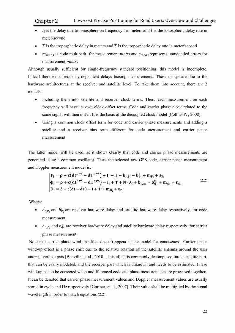
2.1.1 GPS Measurements Model
Classic model for GPS code measurements, carrier phase measurements and Doppler measurements
used in standard positioning is usually [Enge, et al., 2006]:
|
( )
( )
( )
(2.1)
Where
, and are code measurements, carrier phase measurements (in meters) and Doppler (in
meter/second) measurements on frequency respectively
is the true geometric range between satellite and receiver antenna in meters, is the range
rate in meter/second
c is the speed of light
and are receiver and satellite clocks offset with respect to the GPS reference
time, and are receiver and satellite clock offset rate.
22
Low-cost Precise Positioning for Road Users: Overview and Challenges
Chapter 2
is the delay due to ionosphere on frequency in meters and is the ionospheric delay rate in
meter/second
is the tropospheric delay in meters and is the tropospheric delay rate in meter/second
is code multipath for measurement and represents unmodelled errors for
measurement .
Although usually sufficient for single-frequency standard positioning, this model is incomplete.
Indeed there exist frequency-dependent delays biasing measurements. These delays are due to the
hardware architectures at the receiver and satellite level. To take them into account, there are 2
models:
Including them into satellite and receiver clock terms. Then, each measurement on each
frequency will have its own clock offset terms. Code and carrier phase clock related to the
same signal will then differ. It is the basis of the decoupled clock model [Collins P. , 2008].
Using a common clock offset term for code and carrier phase measurements and adding a
satellite and a receiver bias term different for code measurement and carrier phase
measurement.
The latter model will be used, as it shows clearly that code and carrier phase measurements are
generated using a common oscillator. Thus, the selected raw GPS code, carrier phase measurement
and Doppler measurement model is:
|
( )
( )
( )
(2.2)
Where:
and
are receiver hardware delay and satellite hardware delay respectively, for code
measurement.
and
are receiver hardware delay and satellite hardware delay respectively, for carrier
phase measurement.
Note that carrier phase wind-up effect doesn’t appear in the model for conciseness. Carrier phase
wind-up effect is a phase shift due to the relative rotation of the satellite antenna around the user
antenna vertical axis [Banville, et al., 2010]. This effect is commonly decomposed into a satellite part,
that can be easily modeled, and the receiver part which is unknown and needs to be estimated. Phase
wind-up has to be corrected when undifferenced code and phase measurements are processed together.
It can be denoted that carrier phase measurement values and Doppler measurement values are usually
stored in cycle and Hz respectively [Gurtner, et al., 2007]. Their value shall be multiplied by the signal
wavelength in order to match equations (2.2).

23
Low-cost Precise Positioning for Road Users: Overview and Challenges
Chapter 2
2.1.2 GLONASS Measurement Model
The FDMA structure of GLONASS signals implies some differences with GPS measurements. Each
satellite transmits on carrier with different frequencies and the frequency plan for L1 signals is
[Angrisano, 2010]:
(2.3)
Where:
is the GLONASS frequency number. It is an integer between -7 and +6
is the frequency of the satellite with the kth GLONASS frequency number on the sub-
band L1
is the L1 sub-band central frequencies equal to 1602 MHZ.
is the frequency increment equal to 562.5 kHz.
Therefore, it can be deduced that:
The wavelength associated to Doppler and carrier phase measurements are different on each
satellite.
Inter-channel biases can exist. As each GLONASS satellite signal is broadcasted at different
frequency, they go through different paths in the HF part of the transmitter and receiver and
therefore undergo a different hardware delay. It results in biases on code and carrier phase
measurements that are both satellite and receiver dependent.
The GLONASS code, carrier phase measurement and Doppler measurement model is:
|
( )
( )
( )
(2.4)
Where:
and are receiver and satellite clocks offset with respect to the GLONASS
reference time, while and are receiver and satellite clocks offset rate
respectively.
and
are receiver hardware bias and receiver inter-channel biases respectively, for
code measurement
and
are receiver hardware bias and receiver inter-channel biases respectively, for
carrier phase measurement
It can be denoted that the receiver clock rate is in general common to both GPS and GLONASS
Doppler measurements, as they are usually derived from a same receiver oscillator.

24
Low-cost Precise Positioning for Road Users: Overview and Challenges
Chapter 2
2.2 Precise Positioning Techniques (PPP and RTK)
As presented in the previous section, carrier phase ambiguity is easy to model as it is constant if the
phase lock loop tracking is continuous. However, carrier phase ambiguities estimation directly from
raw single-frequency carrier phase measurements and broadcast ephemeris is impossible. Indeed
slowly changing biases such as uncorrected ionospheric delay, residual orbit and satellite clock error,
multipath or unmodelled tropospheric delay makes the observability of the ambiguity value stability
very difficult. In order to isolate and estimate carrier phase ambiguities and turn carrier phase
measurements into very precise pseudoranges, these biases have to be removed. There are two ways to
do this:
to difference the observables from the user receiver (or rover) with the measurements from a
reference receiver that is spatially close in order to remove common biases
to remove the biases directly by either using a linear combination between observables, or
estimating them or obtaining their values from an external source.
The first technique is the basis for Real-Time Kinematic (RTK) that uses at least 2 receivers to
estimate the differenced carrier-phase ambiguities. The second technique is the basis for Precise Point
Positioning (PPP) that estimate the receiver coordinates, the zenith tropospheric delay and the carrier-
phase ambiguities from an ionosphere-free carrier phase combination using precise ephemeris.
Ambiguities can then be estimated either directly as integers if the residual unmodelled errors are
small compared to the carrier wavelength or as floats if this is not the case.
The main advantage of estimating ambiguities as integer is the faster convergence time, which is the
time required to reach the ambiguity true value. Indeed, once the float ambiguity vector is close
enough from the true solution, an integer estimation technique can be used to determine the “closest”
integer vector. A description of these techniques can be found in [Kim, et al., 2000] and [Pais, 2011].
The estimated vector then “jumps” from a float value to the correct integer value, instead of slowly
converging towards it.
In the next 2 sub-chapters, PPP and RTK will be presented. Advantages and drawbacks of each
technique will be exposed and the impact of road user environment on the performance will be
explained.
2.2.1 Precise Point Positioning Presentation
As explained earlier, the main biases preventing carrier phase ambiguity to be isolated as a constant
are ionospheric delay, orbit error, satellite clock and tropospheric delay. Broadcasted navigation data
ephemeris are not precise enough to correct for these errors, as the network used to estimate broadcast
corrections is composed of only a few stations around the world. However, a number of organizations
including the IGS [Dow, et al., 2009] provide more accurate corrections estimated using a larger
network of stations, in real-time or for post-processing purposes. These corrections have the advantage
25
Low-cost Precise Positioning for Road Users: Overview and Challenges
Chapter 2
to require very low bandwidth and can be applied whatever the distance between the user and the
closest reference station.
Constant efforts have been made to improve the accuracy of these products in the past years. In
particular, real-time clock and orbit products with decimeter accuracy are now freely available through
the IGS Real-time service [Agrotis, et al., 2012]. A table comparing a few commercial real-time PPP
products can be found in [Takasu, 2011].
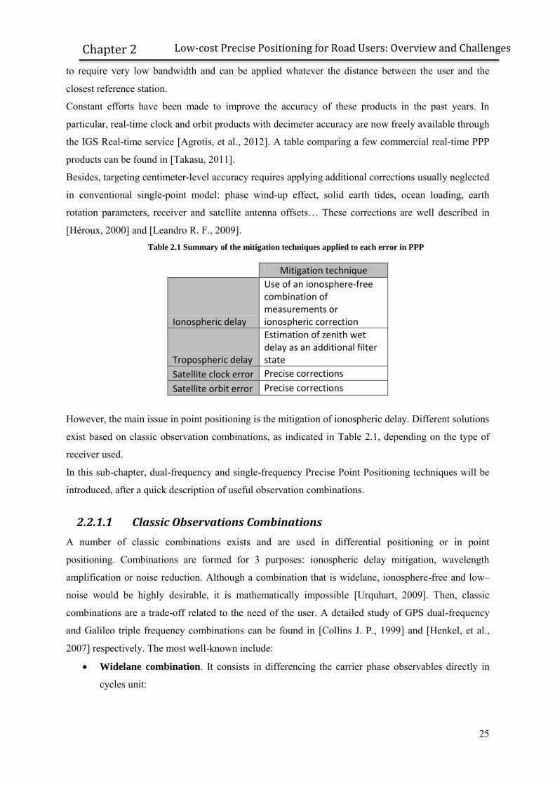
Besides, targeting centimeter-level accuracy requires applying additional corrections usually neglected
in conventional single-point model: phase wind-up effect, solid earth tides, ocean loading, earth
rotation parameters, receiver and satellite antenna offsets… These corrections are well described in
[Héroux, 2000] and [Leandro R. F., 2009]. Table 2.1 Summary of the mitigation techniques applied to each error in PPP
Mitigation technique
Ionospheric delay
Use of an ionosphere-free combination of measurements or ionospheric correction
Tropospheric delay
Estimation of zenith wet delay as an additional filter state
Satellite clock error Precise corrections
Satellite orbit error Precise corrections
However, the main issue in point positioning is the mitigation of ionospheric delay. Different solutions
exist based on classic observation combinations, as indicated in Table 2.1, depending on the type of
receiver used.
In this sub-chapter, dual-frequency and single-frequency Precise Point Positioning techniques will be
introduced, after a quick description of useful observation combinations.
2.2.1.1 Classic Observations Combinations
A number of classic combinations exists and are used in differential positioning or in point
positioning. Combinations are formed for 3 purposes: ionospheric delay mitigation, wavelength
amplification or noise reduction. Although a combination that is widelane, ionosphere-free and low–
noise would be highly desirable, it is mathematically impossible [Urquhart, 2009]. Then, classic
combinations are a trade-off related to the need of the user. A detailed study of GPS dual-frequency
and Galileo triple frequency combinations can be found in [Collins J. P., 1999] and [Henkel, et al.,
2007] respectively. The most well-known include:
Widelane combination. It consists in differencing the carrier phase observables directly in
cycles unit:

26
Low-cost Precise Positioning for Road Users: Overview and Challenges
Chapter 2
| (
)
( )
( )
(2.5)
It creates an observable that has the same geometrical properties than L1 and L2 double
differenced observables but with a longer wavelength
(
) . is
then called the wide-lane ambiguity.
Narrowlane code combination.
| (
)
( )
(2.6)
Assuming and have similar level of noise, is √(
) (
)
less noisy than .
The ionospheric delay of the widelane carrier-phase equals the ionospheric delay of the
narrowlane code [Banville, et al., 2008].
Melbourne-Wübbena combination. This combination uses the widelane phase combination
in meters and the narrowlane code combination: ( )
This combination is very useful to isolate and solve the widelane ambiguity.
Ionosphere-free combination. It consists in removing the first order of the ionospheric delay,
while keeping the other effects unchanged. For dual frequency L1/L2 code measurements:
|
( )
(2.7)
where
and
The same combination can be formed with carrier-phase observables:
|
( )
(2.8)
GRAPHIC (GRoup And Phase Ionospheric Correction), usually performed on L1
measurements:
( )
(2.9)
This combination is ionosphere-free but ambiguous. The noise level is half the code noise.
2.2.1.2 Dual-frequency PPP
If dual-frequency measurements are available, the so-called ionosphere-free combination can be used
to cancel out the first order of the ionospheric delay, while keeping the other effects unchanged.

27
Low-cost Precise Positioning for Road Users: Overview and Challenges
Chapter 2
By cancelling satellite clock offset using corrections provided by the IGS to observations, i.e. related
to dual-frequency code measurements and assuming a perfect correction, the following system can be
obtained:
|
(2.10)
Where:
is the satellite clock correction related to dual-frequency code measurements
As seen on equation (2.10), satellite hardware biases remain in carrier phase measurements after
applying ephemeris corrections. This is due to the fact that satellite clock offset using corrections
provided by the IGS only correct for code satellite hardware biases. More details on the subtleties of
ephemeris corrections are given in Appendix A.
Conventional PPP software uses Equations (2.10) as input observations in a Kalman filter, estimating
antenna coordinates, tropospheric delay, a common clock term for code and carrier phase
measurement and a constant float term biasing carrier phase measurement [Witchayangkoon, 2000].
More recently, new techniques have been proposed to explicitly correct for carrier phase satellite
hardware biases in order to completely isolate the carrier phase ambiguities from other biases and
estimate it as an integer. Different parameterizations models have been proposed in [Laurichesse, et
al., 2009], [Collins P. , 2008] and [Ge, et al., 2008]. Methods are however very similar.
To estimate the undifferenced L1 ambiguities as an integer, a method is proposed in [Laurichesse, et
al., 2009]. It is based on the use of satellite clock products that keep the integer property of the
narrowlane ambiguity in the ionosphere-free carrier phase combination and a set of Melbourne-
Wübbena satellite biases. To summarize, it is performed in 4 steps:
Estimation of the widelane ambiguities. This step is performed by subtracting Melbourne-
Wübbena satellite biases from the Melbourne-Wübbena combination and averaging over a
time window (usually 10 minutes [Laurichesse, et al., 2009]).
Formation of the ionosphere-free carrier phase combination and application of PPP-AR
satellite clock corrections, i.e:
(2.11)
Removal of widelane ambiguities obtained from step 1, i.e.
(2.12)
with and

28
Low-cost Precise Positioning for Road Users: Overview and Challenges
Chapter 2
PPP-processing to determine the integer narrow-lane ambiguities. The integer narrow-
lane ambiguity resolution involves estimating in a Kalman filter:
o the receiver clock term ( ),
o the zenith tropospheric delay, and
o float ambiguities.
Integer ambiguities can be estimated from float ambiguities using for instance the LAMBDA method
[Teunissen P. , 1995] or partial fixing algorithms [Shi, et al., 2012].
The required PPP-AR products can be obtained from different sources. The CNES/CLS IGS center is
providing both the satellite clock bias and the Melbourne-Wübbena satellite biases for post-processing
purposes (GRG products freely available on the IGS website [Perosanz, et al., 2009]). Recently, PPP-
AR products have been available in real-time via Ntrip streams within the PPP-Wizard project
[CNES, 2011]. Indeed, by knowing station position very precisely, reverse processing allows to
estimate centimeter-level satellite clock offset and orbits in real-time [Laurichesse, et al., 2009].
In the case of a single-frequency user, ionospheric delay can be partially or totally mitigated using 3
methods:
The so-called GRAPHIC combination
Use of ionospheric TEC maps.
Using empirical models such as Klobuchar model or NeQuick model. However empirical
model have currently a too low accuracy to be used for PPP.
PPP processing using the first 2 techniques will be described in the next section.
2.2.1.3 Single-frequency PPP
The GRAPHIC combination can be used to determine a precise position using single-frequency
measurements, as in [Beran, 2008] and [Laurichesse, et al., 2009]. The main advantage of the
GRAPHIC combination is that it totally removes the first order ionospheric delay, as seen in equation
(2.9).
Classic PPP uses an ambiguous observable, provided by carrier phase measurements, and a non-
ambiguous observable provided by code measurements. Nonetheless GRAPHIC PPP processing uses
only an ambiguous ionosphere-free combination in a Kalman filter to estimate the position. Multiple
epochs, i.e. long observation period, is required so that satellite geometry change sufficiently to
provide enough observability to the system. Additionally, the GRAPHIC observable is affected by
code multipath and noise which lengthen the convergence time. Altogether, convergence time can
reach a few hours and accuracy remains at decimeter level [Laurichesse, et al., 2009].
A second method for single-frequency user is to use ionospheric Total Electron Content (TEC) maps
for ionospheric delay correction. Ionospheric TEC maps are time-tagged geographical grid of vertical
TEC values that can be interpolated to determine vertical ionospheric delay at a desired location. For

29
Low-cost Precise Positioning for Road Users: Overview and Challenges
Chapter 2
instance the IGS provides a grid, spaced by 2.5 degrees in latitude and 5 degrees in longitude of
Vertical Total Electron Content (VTEC) values every 2 hours. SBAS systems, such as WAAS and
EGNOS are also providing ionospheric grid in real-time, with a precision allowing to obtain
decimeter-level position [Wanninger, et al., 2012].
L1 carrier phase can then be corrected at least partially from ionospheric delay:
( ) ( )
(2.13)
Where:
is the ionospheric delay correction
( ) is the ionospheric correction error
Description of PPP algorithms using ionospheric TEC maps can be found in [Beran, 2008] and
[Muellerschoen, et al., 2004].
There are a number of advantages to use TEC maps instead of GRAPHIC combination for PPP:
The observable used for PPP is not contaminated by code multipath. The final position
accuracy should then be similar on a low-cost receiver and a high grade receiver since only
carrier phase measurements are used.
Free real-time ionospheric grid maps are available in regions covered by SBAS. Their
accuracy is expected to improve in the upcoming years with full GNSS tracking from SBAS
ground segments.
The wavelength associated to the ambiguity is 2 times larger than in the case GRAPHIC
combination is used. Then the search space is reduced in the case ambiguities are estimated as
integers.
However, the residual ionospheric error ( ) left in the carrier phase measurement is a slowly
changing bias which makes it very difficult to separate from the ambiguity term. Additionally,
ionospheric delay correction is usually difficult to weight in the filter, as the variance provided by the
SBAS services are usually overly pessimistic. These drawbacks result in long convergence time and
decimeter-level position.
2.2.2 Real-Time Kinematic Presentation
Atmospheric errors, satellite orbit error or satellite clock offset error are spatially and temporally
correlated errors. It means that 2 closely spaced receivers tracking the same signals at the same time
undergo approximately the same error. Geodesists took advantage of this in the early age of GPS
development to reduce the error budget. By simply differencing measurements from 2 close and
synchronized receivers, spatially correlated errors are eliminated or reduced. It is the basic principle of
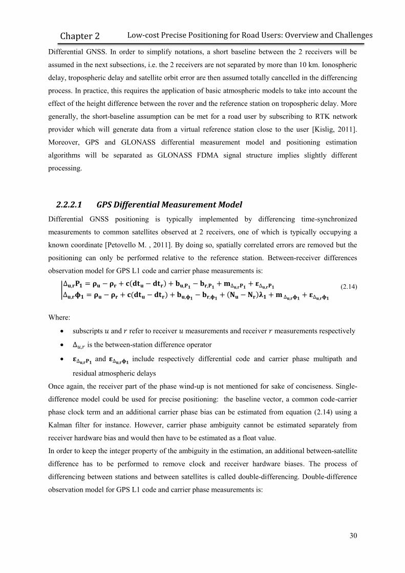
30
Low-cost Precise Positioning for Road Users: Overview and Challenges
Chapter 2
Differential GNSS. In order to simplify notations, a short baseline between the 2 receivers will be
assumed in the next subsections, i.e. the 2 receivers are not separated by more than 10 km. Ionospheric
delay, tropospheric delay and satellite orbit error are then assumed totally cancelled in the differencing
process. In practice, this requires the application of basic atmospheric models to take into account the
effect of the height difference between the rover and the reference station on tropospheric delay. More
generally, the short-baseline assumption can be met for a road user by subscribing to RTK network
provider which will generate data from a virtual reference station close to the user [Kislig, 2011].
Moreover, GPS and GLONASS differential measurement model and positioning estimation
algorithms will be separated as GLONASS FDMA signal structure implies slightly different
processing.
2.2.2.1 GPS Differential Measurement Model
Differential GNSS positioning is typically implemented by differencing time-synchronized
measurements to common satellites observed at 2 receivers, one of which is typically occupying a
known coordinate [Petovello M. , 2011]. By doing so, spatially correlated errors are removed but the
positioning can only be performed relative to the reference station. Between-receiver differences
observation model for GPS L1 code and carrier phase measurements is:
| ( )
( )
( )
(2.14)
Where:
subscripts and refer to receiver measurements and receiver measurements respectively
is the between-station difference operator
and
include respectively differential code and carrier phase multipath and
residual atmospheric delays
Once again, the receiver part of the phase wind-up is not mentioned for sake of conciseness. Single-
difference model could be used for precise positioning: the baseline vector, a common code-carrier
phase clock term and an additional carrier phase bias can be estimated from equation (2.14) using a
Kalman filter for instance. However, carrier phase ambiguity cannot be estimated separately from
receiver hardware bias and would then have to be estimated as a float value.
In order to keep the integer property of the ambiguity in the estimation, an additional between-satellite
difference has to be performed to remove clock and receiver hardware biases. The process of
differencing between stations and between satellites is called double-differencing. Double-difference
observation model for GPS L1 code and carrier phase measurements is:

31
Low-cost Precise Positioning for Road Users: Overview and Challenges
Chapter 2
|
(2.15)
Where:
is the double difference operator
(
) (
) is the double difference range between station and and
between satellite and
(
) (
) is the double difference integer ambiguity on L1 carrier
phase between station and and between satellite and
It can be denoted that only carrier phase double differencing is required to keep the integer property of
carrier phase ambiguity. Code measurements can be kept in single-difference mode, as seen on
equation (2.16):
|
(2.16)
Where:
( )
is the “equivalent clock” term that is common to all GPS
code measurements
In this case, baseline vector, equivalent clock term and integer ambiguities can be estimated together
in a Kalman filter. Equation (2.15) and equation (2.16) are equivalent from a position estimation point
of view, provided the correlation implied by between-satellite differencing is properly taken into
account in the observation covariance matrix. However it will be shown in 4.2.1.1 that keeping code
measurements in single-difference form can be advantageous.
2.2.2.2 GLONASS Differential Measurement Model
Differential GLONASS has recently gained attention with the significant improvement in GLONASS
accuracy and availability over the past 5 years. The between-receiver difference observation model for
GLONASS code and carrier phase measurements on frequency is:
| ( )
( )
(2.17)
Where:
and
are receiver and inter-channel biases
differences on code measurements
and
are receiver and inter-channel biases
differences on carrier phase measurements
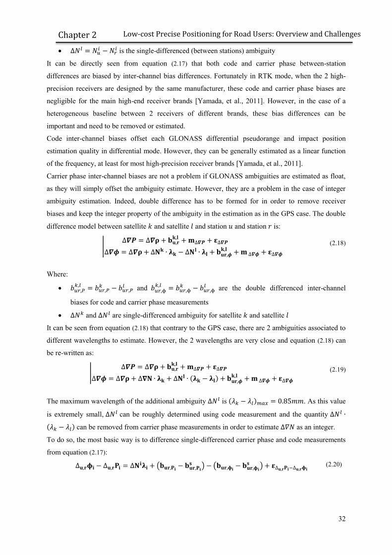
32
Low-cost Precise Positioning for Road Users: Overview and Challenges
Chapter 2
is the single-differenced (between stations) ambiguity
It can be directly seen from equation (2.17) that both code and carrier phase between-station
differences are biased by inter-channel bias differences. Fortunately in RTK mode, when the 2 high-
precision receivers are designed by the same manufacturer, these code and carrier phase biases are
negligible for the main high-end receiver brands [Yamada, et al., 2011]. However, in the case of a
heterogeneous baseline between 2 receivers of different brands, these bias differences can be
important and need to be removed or estimated.
Code inter-channel biases offset each GLONASS differential pseudorange and impact position
estimation quality in differential mode. However, they can be generally estimated as a linear function
of the frequency, at least for most high-precision receiver brands [Yamada, et al., 2011].
Carrier phase inter-channel biases are not a problem if GLONASS ambiguities are estimated as float,
as they will simply offset the ambiguity estimate. However, they are a problem in the case of integer
ambiguity estimation. Indeed, double difference has to be formed for in order to remove receiver
biases and keep the integer property of the ambiguity in the estimation as in the GPS case. The double
difference model between satellite and satellite and station and station is:
|
(2.18)
Where:
and
are the double differenced inter-channel
biases for code and carrier phase measurements
and are single-differenced ambiguity for satellite and satellite
It can be seen from equation (2.18) that contrary to the GPS case, there are 2 ambiguities associated to
different wavelengths to estimate. However, the 2 wavelengths are very close and equation (2.18) can
be re-written as:
|
( )
(2.19)
The maximum wavelength of the additional ambiguity is ( ) . As this value
is extremely small, can be roughly determined using code measurement and the quantity
( ) can be removed from carrier phase measurements in order to estimate as an integer.
To do so, the most basic way is to difference single-differenced carrier phase and code measurements
from equation (2.17):
(
) (
) (2.20)
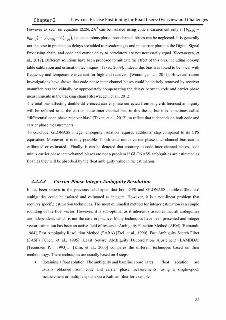
33
Low-cost Precise Positioning for Road Users: Overview and Challenges
Chapter 2
However as seen on equation (2.20), can be isolated using code measurement only if (
) (
), i.e. code minus phase inter-channel biases can be neglected. It is generally
not the case in practice, as delays are added to pseudoranges and not carrier phase in the Digital Signal
Processing chain, and code and carrier delay to correlators are not necessarily equal [Sleewaegen, et
al., 2012]. Different solutions have been proposed to mitigate the effect of this bias, including look-up
table calibration and estimation techniques [Takac, 2009]. Indeed, this bias was found to be linear with
frequency and temperature invariant for high-end receivers [Wanninger L. , 2011]. However, recent
investigations have shown that code-phase inter-channel biases could be entirely removed by receiver
manufacturers individually by appropriately compensating the delays between code and carrier phase
measurements in the tracking chain [Sleewaegen, et al., 2012].
The total bias affecting double-differenced carrier phase corrected from single-differenced ambiguity
will be referred to as the carrier phase inter-channel bias in this thesis, but it is sometimes called
“differential code-phase receiver bias” [Takac, et al., 2012], to reflect that it depends on both code and
carrier phase measurements.
To conclude, GLONASS integer ambiguity isolation requires additional step compared to its GPS
equivalent. Moreover, it is only possible if both code minus carrier phase inter-channel bias can be
calibrated or estimated. Finally, it can be denoted that contrary to code inter-channel biases, code
minus carrier phase inter-channel biases are not a problem if GLONASS ambiguities are estimated as
float, as they will be absorbed by the float ambiguity value in the estimation.
2.2.2.3 Carrier Phase Integer Ambiguity Resolution
It has been shown in the previous subchapter that both GPS and GLONASS double-differenced
ambiguities could be isolated and estimated as integers. However, it is a non-linear problem that
requires specific estimation techniques. The most minimalist method for integer estimation is a simple
rounding of the float vector. However, it is sub-optimal as it inherently assumes that all ambiguities
are independent, which is not the case in practice. Many techniques have been presented and integer
vector estimation has been an active field of research: Ambiguity Function Method (AFM) [Remondi,
1984], Fast Ambiguity Resolution Method (FARA) [Frei, et al., 1990], Fast Ambiguity Search Filter
(FASF) [Chen, et al., 1995], Least Square AMBiguity Decorrelation Ajustement (LAMBDA)
[Teunissen P. , 1993]… [Kim, et al., 2000] compares the different techniques based on their
methodology. These techniques are usually based on 4 steps:
Obtaining a float solution. The ambiguity and baseline coordinates float solution are
usually obtained from code and carrier phase measurements, using a single-epoch
measurement or multiple epochs via a Kalman filter for example.

34
Low-cost Precise Positioning for Road Users: Overview and Challenges
Chapter 2
Defining a search volume. The search domain can be in the position domain, the ambiguity
domain or the measurement domain [Kim, et al., 2000].
Defining a cost function and a grid in the search volume to find the point that minimizes the
cost function.
Validating the ambiguity set. This step is of critical importance since a cost function local
minimum can always be found. However, a decision has to be made whether this point can be
accepted or rejected. Different methods exist such as the ratio-test [Teunissen, et al., 2007] or
the margin test [Nagano, et al., 2005].
Once the integer ambiguity vector has been accepted, the baseline vector obtained from float
estimation can be adjusted to match with the integer ambiguity vector.
Factors influencing the speed and success rate of the ambiguity resolution:
Code measurement quality [Kubo, et al., 2006].
Amplitude of double-differenced carrier phase residuals [Milbert, 2005]. High residuals can be
due to residual atmospheric delay, carrier phase multipath or GLONASS inter-channel biases.
Important carrier phase residuals can lead to wrong integer vector estimation or prevent the
ambiguity from being validated.
The use of measurements from different frequencies [Milbert, 2005]. Using dual-frequency or
triple-frequency measurements dramatically reduces the ambiguity search space.
In order to determine the challenges associated to precise vehicular navigation, different types of
environment typically encountered by a land vehicle will be presented in the next section. Moreover,
measurements obtained from a real data collection are analyzed.
2.3 Road User Environment Characteristics
In order to reach sub-meter to centimeter accuracy, precise positioning techniques presented in the
previous section shall be used. However these techniques were initially developed for clear-sky
environments and low dynamic conditions. Therefore it is all the more difficult to use them for land
vehicular navigation as a wide range of propagation channels can be experienced. It goes from a near-
clear sky environment on a highway to the low satellite visibility and high multipath environment
found in downtown urban canyon. Additionally, the quality of the data-link in the targeted
environment (latency, bit rate…) also has to be taken into account as precise positioning techniques
require additional corrections. Different types of data link can be used: radio link, satcom, cell phone
network… As the area of coverage required for land vehicle navigation can be potentially large, a cost
efficient solution for the data link chosen in this PhD study is to use the mobile telecommunication
network.
Details on road user environments characteristics will be given in the next 2 sub-sections.
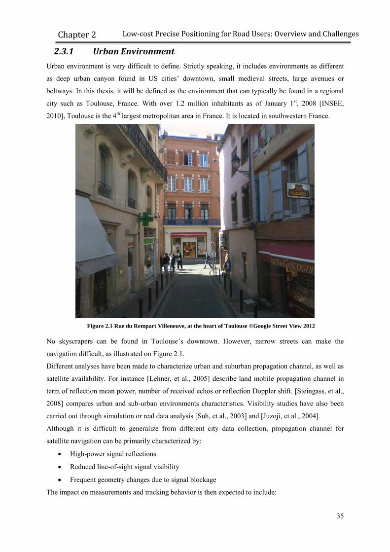
35
Low-cost Precise Positioning for Road Users: Overview and Challenges
Chapter 2
2.3.1 Urban Environment
Urban environment is very difficult to define. Strictly speaking, it includes environments as different
as deep urban canyon found in US cities’ downtown, small medieval streets, large avenues or
beltways. In this thesis, it will be defined as the environment that can typically be found in a regional
city such as Toulouse, France. With over 1.2 million inhabitants as of January 1st, 2008 [INSEE,
2010], Toulouse is the 4th largest metropolitan area in France. It is located in southwestern France.
Figure 2.1 Rue du Rempart Villeneuve, at the heart of Toulouse ©Google Street View 2012
No skyscrapers can be found in Toulouse’s downtown. However, narrow streets can make the
navigation difficult, as illustrated on Figure 2.1.
Different analyses have been made to characterize urban and suburban propagation channel, as well as
satellite availability. For instance [Lehner, et al., 2005] describe land mobile propagation channel in
term of reflection mean power, number of received echos or reflection Doppler shift. [Steingass, et al.,
2008] compares urban and sub-urban environments characteristics. Visibility studies have also been
carried out through simulation or real data analysis [Suh, et al., 2003] and [Juzoji, et al., 2004].
Although it is difficult to generalize from different city data collection, propagation channel for
satellite navigation can be primarily characterized by:
High-power signal reflections
Reduced line-of-sight signal visibility
Frequent geometry changes due to signal blockage
The impact on measurements and tracking behavior is then expected to include:

36
Low-cost Precise Positioning for Road Users: Overview and Challenges
Chapter 2
Significant multipath error on measurements, notably pseudoranges and Doppler
measurements.
Non-Line-of-Sight (NLOS) signal tracking
Frequent cycle slips and loss of lock for carrier phase measurements
As explained earlier, both PPP and RTK techniques require additional precise corrections to be
transmitted in real-time to the user. As mobile network coverage in French cities is usually very good,
the data-link is then anticipated to be low-latency and have a high data-rate.
2.3.2 Rural Environment
Similarly to urban environment, it is difficult to encompass rural environment in a single description.
It can include forest tracks, highways or mountain secondary roads, each of these environments having
very different propagation channel. However, it can be generally characterized by:
Good satellite geometry
Potentially attenuated signals due to tree foliage
Multipath mostly caused by ground reflection. Lower power reflections can then be expected,
compared to urban environment.
This environment is usually considered as more favorable to satellite navigation compared to deep
urban environment. However, signals can be heavily attenuated which can impact receiver tracking
quality and reduce resistance to multipath. Moreover cellphone network coverage is worse than in
urban area. For instance [Yang, et al., 2010] point out that local tests on UK roads have shown that
even on the highway roads, the cell phone network cannot be guaranteed.
2.3.3 Road User Dynamic
In the targeted applications, the receiver antenna can be assumed mounted on the roof of a car, driven
at traffic speed on French roads. In these conditions, the velocity of the receiver antenna in the plane
perpendicular to the forward direction (x-axis), i.e. the speed in the up direction (z-axis) and in the
direction of the rear axle (y-axis), is then almost zero. These restrictions on the vehicle motion are
called non-holonomic constraints [Sukkarieh, 2000]. Moreover, a road user is expected to have a
velocity range from 0 to 130km/h, as it is the maximum speed limit in France. In term of acceleration,
typical behavior for a land vehicle was reported to range from -1.5 m.s-2 to 3.7 m.s-2 in [Ahn, et al.,
2002].
2.4 Real Data Analysis
In this section, real data from a measurement campaign performed in spring 2009 are analyzed to
refine the previous propagation channels descriptions. The goal of this data analysis is to give a first

37
Low-cost Precise Positioning for Road Users: Overview and Challenges
Chapter 2
idea of the different phenomenon that can be encountered in different road user environment, in term
of measurement accuracy and measurement availability.
During the measurement campaign, a uBlox LEA-4T [uBlox, 2007] was connected to a patch antenna
ANN-MS [uBlox, 2011], and mounted on the roof of a car. The uBlox LEA-4T is a single-frequency
low-cost receiver tracking GPS-only satellites. This receiver delivers raw data, i.e. code, Doppler
carrier phase and C/N0 measurements. The receiver and the patch antenna have a total cost of a few
dozens euros, which makes it suitable for the type of targeted application. 4Hz data was collected and
analyzed in 3 types of environment: a rural road surrounded by forest near Biscarosse, Bordeaux’s
beltway (peri-urban environment) and Lyon’s downtown (urban environment). Lyon and Bordeaux are
respectively the 3rd and the 9th most populated cities in France. The reference trajectory was post-
processed using data from a Novatel DLV3 GPS/GLONASS L1/L2 receiver and a LandINS FOG
IMU from IXSea [IXSEA]. Reference trajectory accuracy was at sub-meter level. In each
environment, data was collected during 4 sessions at different time of the day, following
approximately the same route. Sessions from a same environment were then combined in order to
compute statistics. A total of approximately 2 hours, 4 hours and 3 hours data were collected for
Biscarosse, Bordeaux’s beltway and Downtown Lyon. Trajectories can be found on Figure 2.2, Figure
2.3 and Figure 2.4.
Figure 2.2 Trajectory of the vehicle on Bordeaux’s beltway
Figure 2.3 Trajectory of the vehicle in downtown Lyon
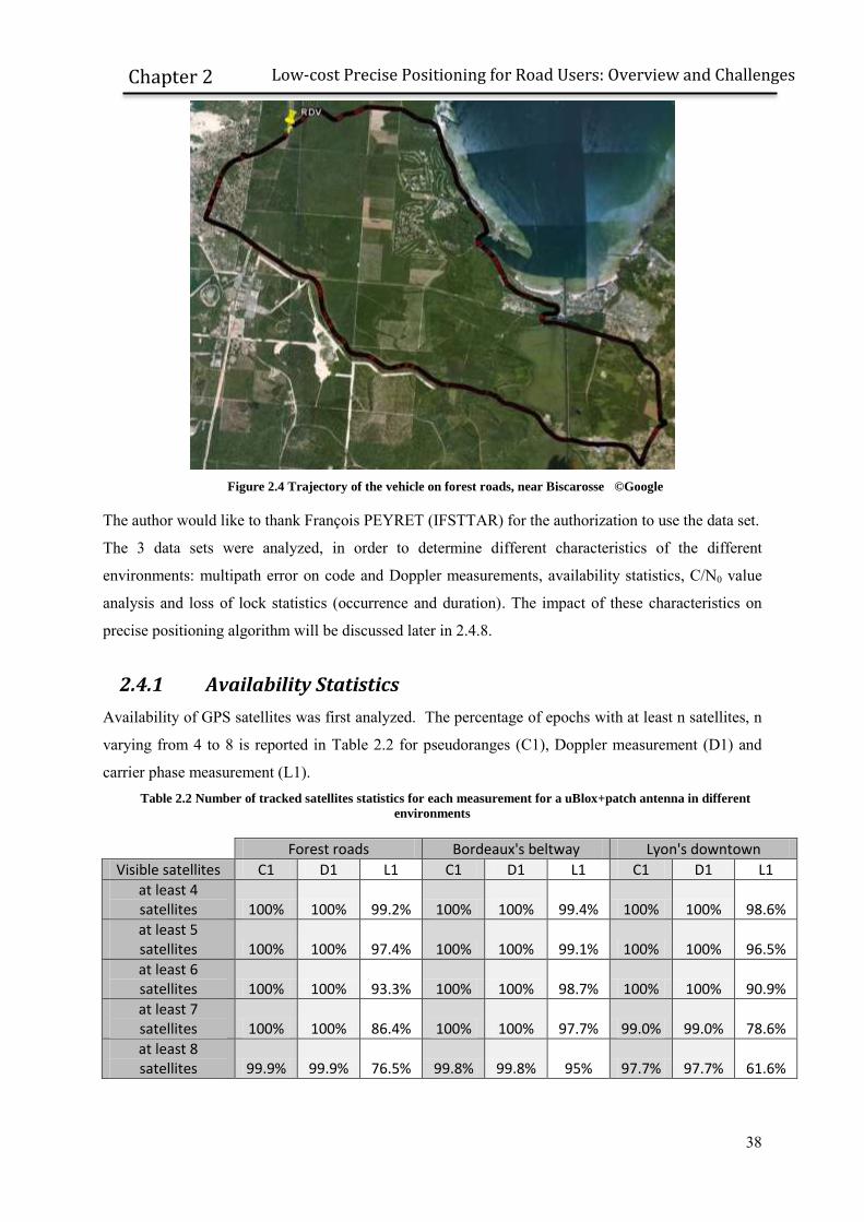
38
Low-cost Precise Positioning for Road Users: Overview and Challenges
Chapter 2
Figure 2.4 Trajectory of the vehicle on forest roads, near Biscarosse ©Google
The author would like to thank François PEYRET (IFSTTAR) for the authorization to use the data set.
The 3 data sets were analyzed, in order to determine different characteristics of the different
environments: multipath error on code and Doppler measurements, availability statistics, C/N0 value
analysis and loss of lock statistics (occurrence and duration). The impact of these characteristics on
precise positioning algorithm will be discussed later in 2.4.8.
2.4.1 Availability Statistics
Availability of GPS satellites was first analyzed. The percentage of epochs with at least n satellites, n
varying from 4 to 8 is reported in Table 2.2 for pseudoranges (C1), Doppler measurement (D1) and
carrier phase measurement (L1). Table 2.2 Number of tracked satellites statistics for each measurement for a uBlox+patch antenna in different
environments
Forest roads Bordeaux's beltway Lyon's downtown
Visible satellites C1 D1 L1 C1 D1 L1 C1 D1 L1
at least 4 satellites 100% 100% 99.2% 100% 100% 99.4% 100% 100% 98.6%
at least 5 satellites 100% 100% 97.4% 100% 100% 99.1% 100% 100% 96.5%
at least 6 satellites 100% 100% 93.3% 100% 100% 98.7% 100% 100% 90.9%
at least 7 satellites 100% 100% 86.4% 100% 100% 97.7% 99.0% 99.0% 78.6%
at least 8 satellites 99.9% 99.9% 76.5% 99.8% 99.8% 95% 97.7% 97.7% 61.6%

39
Low-cost Precise Positioning for Road Users: Overview and Challenges
Chapter 2
It can be seen that code measurement availability is very good in the 3 environments. This result could
be expected as the uBlox LEA-4T is a high-sensitivity receiver. Additionally, it can be denoted that
Doppler measurements have a significantly higher availability than carrier phase measurements, their
availability being as high as pseudoranges availability. Moreover, availability of carrier phase
measurements is significantly worse on forest roads than on Bordeaux’s beltway, while pseudorange
measurements availability in both environments is similar. It can come from the fact that trees and
foliage close to the road attenuates the signal coming from satellites. As phase lock loop has a higher
tracking loss threshold than delay lock loop, the satellite signal might be sufficiently strong to track
code measurement but too weak to keep carrier phase lock. However, the availability of at least 5
carrier phase measurements remains over 95% in all environments. Therefore precise positioning
techniques are theoretically available in these environments, provided measurements accuracy is
sufficient.
In order to determine the quality of the received signal, the cumulative density function of C/N0 values
as provided by the receiver is plotted on Figure 2.5 for the different environments.
Figure 2.5 Cumulative density function of C/N0 values, in different environments using a uBlox LEA-4T
connected to a patch antenna
C/N0 provides an indication of the signal power of the tracked satellite and the noise density as seen by
the receiver’s front-end [Joseph, 2010]. A low C/N0 can come from signal attenuation due to the
environment, multipath effect [Brown, 2000], NLOS tracking or low elevation of the tracked satellite.
As expected from availability statistics, C/N0 values are clearly lower in downtown Lyon and on rural
roads than on Bordeaux’s beltway, which may be the cause of carrier loss of lock. More than 34% of
measurements are below 40 dB.Hz for the data set from downtown Lyon, whereas only 21% are below
40dB.Hz on Bordeaux’s beltway. Additionally, more than 23% of measurements have a C/N0 value
lower than 35dB.Hz in downtown Lyon, which may indicate that receiver is tracking highly-attenuated
20 25 30 35 40 45 500
0.1
0.2
0.3
0.4
0.5
0.6
0.7
0.8
0.9
1
C/N0 (dB.Hz)
Cum
ula
tive d
istr
ibution f
unction
Cumulative distribution function of C/N0 values
Rural roads
Bordeaux's beltway
Downtown Lyon

40
Low-cost Precise Positioning for Road Users: Overview and Challenges
Chapter 2
NLOS signals. Approximately 28% of the measurements have a C/N0 value of less than 40dB.Hz on
rural roads, reflecting the high signal attenuation due to tree foliage.
In order to see the effect of the environment on measurement error, code multipath and Doppler
multipath are analyzed in the next 2 sections.
2.4.2 Code Multipath Error Analysis
In order to isolate multipath error, code double differences were formed between uBlox measurements
and close reference station from the RGP network [IGN, 2012]. Then, double-differenced range
computed using reference trajectory and base station coordinates was subtracted from double
difference code measurements to isolate the combined effect of multipath and noise error. The satellite
with the highest C/N0 value on the uBlox was chosen as reference satellite to form the double
difference. No elevation or C/N0 mask was applied and differential tropospheric delay was corrected
using UNB3m model [Leandro R. F., 2009]. Results can be found for the 3 environments on Figure
2.6. It can clearly be seen that most error over 20 meters are positive, notably for the urban data set. It
is due to NLOS signal tracking which cause only positive error, as a signal reflection always travels a
longer path than the direct signal.
Figure 2.6 Code double difference multipath error between a uBlox LEA-4T and reference stations from the
RGP network. Each color is a different satellite pair.
0 0.5 1 1.5 2 2.5 3
x 104
-100
-80
-60
-40
-20
0
20
40
60
80
100Code Double-differenced residuals (Forest roads)
epochs (4Hz data)
mete
rs
0 1 2 3 4 5
x 104
-100
-80
-60
-40
-20
0
20
40
60
80
100Code Double-differenced residuals (Bordeaux's beltway)
epochs (4Hz data)
mete
rs
0 0.5 1 1.5 2 2.5 3 3.5 4 4.5 5
x 104
-100
-80
-60
-40
-20
0
20
40
60
80
100Code Double-differenced residuals (Lyon's downtown)
epochs (4Hz data)
mete
rs

41
Low-cost Precise Positioning for Road Users: Overview and Challenges
Chapter 2
This makes the mean of the multipath error clearly positive in the case of the data set from downtown
Lyon, as seen in Table 2.3. In the case of forest roads and Bordeaux’s beltway, the multipath error
seems almost centered. An explanation is that the phase of the multipath changes quickly, as the
speed of the vehicle is typically high in these environments. Therefore, multipaths tend to have a
noise-like behavior at high speed, provided the LOS is tracked.
Code measurement error standard deviation is higher in Biscarosse data set than on Bordeaux’s
beltway, as indicated in Table 2.3, probably caused by signal attenuation due to tree foliage. Table 2.3 Estimated mean and standard deviation of code measurement error in the different environments
Forest road Bordeaux's beltway Lyon's downtown
Mean 0.30 meters 0.33 meters 4.70 meters
Standard deviation 5.37 meters 3.89 meters 15.34 meters
2.4.3 Doppler Multipath Error Analysis
Similarly to code measurements, combined effect of noise and multipath error on Doppler
measurements can be isolated by removing Doppler due to satellite and receiver velocity.
Additionally, a single-difference (between satellites) has to be performed to cancel Doppler due to
clock bias rate. Doppler measurement errors in the different environments are plotted on Figure 2.7,
together with receiver velocity. It can be seen that Doppler multipath error can reach a few
meters/seconds.

42
Low-cost Precise Positioning for Road Users: Overview and Challenges
Chapter 2
Figure 2.7 between-satellite difference of Doppler measurement error between a uBlox LEA-4T. Each color is a
different satellite pair. Reference velocity norm is plotted in blue at the bottom.
Moreover, a clear correlation with receiver speed exists. Indeed, the Doppler measurement multipath
error is null for a static receiver surrounded by a static environment, as the frequency of the direct
signal and the frequency of the reflected signal are then equal. Additionally, it can be seen that
multipath error is in general bounded by receiver speed and can be either positive or negative.
However multipath error can theorically exceed receiver speed in a few cases, in the case of a
reflection with a vehicle driving in the opposite direction.
In the 3 types of environment, Doppler multipath error was found to be almost zero-mean, as seen on
Table 2.4. Table 2.4 Estimated mean and standard deviation of Doppler measurement error in the different environments
Forest road Bordeaux's beltway Lyon's downtown
Mean 0.00 meters/seconds 0.00 meters/seconds -0.01 meters/seconds
Standard deviation 1.12 meters/seconds 0.77 meters/seconds 1.43 meters/seconds
0 0.5 1 1.5 2 2.5 3
x 104
-30
-20
-10
0
10
20
30Forest roads
epochs
Dopple
r S
ingle
-diffe
renced (
betw
een s
ate
llite
) m
ultip
ath
(m
/s)
0 0.5 1 1.5 2 2.5 3
x 104
0
5
10
15
20
25
30
Refe
rence v
elo
city n
orm
(m
/s)
0 1 2 3 4 5
x 104
-30
-20
-10
0
10
20
30Bordeaux's beltway
epochs
Dopple
r S
ingle
-diffe
renced (
betw
een s
ate
llite
) m
ultip
ath
(m
/s)
0 1 2 3 4 5
x 104
0
20
40
Refe
rence v
elo
city n
orm
(m
/s)
0 0.5 1 1.5 2 2.5 3 3.5 4 4.5 5
x 104
-30
-20
-10
0
10
20
30Downtown Lyon
epochs
Dopple
r S
ingle
-diffe
renced (
betw
een s
ate
llite
) m
ultip
ath
(m
/s)
0 0.5 1 1.5 2 2.5 3 3.5 4 4.5 5
x 104
0
20
40
Refe
rence v
elo
city n
orm
(m
/s)

43
Low-cost Precise Positioning for Road Users: Overview and Challenges
Chapter 2
2.4.4 Carrier Phase Measurement Analysis
Code measurement and Doppler measurement have a level of noise and multipath at least at the
decimeter-level and decimeter/second-level respectively in kinematic mode. However, carrier phase
multipath error is bounded by a quarter of the wavelength when the reflected signal’s amplitude is less
than that of the direct signal [Langley R. B., 2011]. It is then very difficult to isolate carrier phase
multipath error from a kinematic data set unless a sub-centimeter accurate reference trajectory is
available. However, other characteristics of interest for carrier phase positioning can be deduced from
the different environment data sets. In particular, the occurrence and duration of carrier phase loss of
lock can be analyzed. They can be seen as an indicator of the time available to fix carrier phase
ambiguities or to smooth code measurement with carrier phase measurements. Cumulative density
function of the duration of carrier phase tracking losses, as well as the duration between 2 tracking
losses are plotted on Figure 2.8 and Figure 2.9 for the different environments. In these statistics, a loss
of lock is a carrier phase unavailability while the satellite elevation is above 15°.
Figure 2.8 Estimated cumulative density function of a loss of
lock’s duration in the different environments
Figure 2.9 Estimated cumulative density function of the
duration between 2 consecutive loss of lock
As it can be seen, loss of lock duration is usually very short. 85% last less than 4 seconds in urban
environment, whereas this percentage reaches 95% on Bordeaux’s beltway and rural roads. Carrier
phase tracking outages last longer in downtown Lyon, probably due to street buildings signal
blockage. Secondly, the duration between 2 consecutive carrier phase tracking outages is also very
short for rural roads and downtown Lyon. In particular, 83% and 88% of losses of locks are separated
by a maximum of 5 seconds in downtown Lyon and rural roads. It can be concluded that very frequent
losses of lock of short duration have to be expected in these environments. Conclusions on carrier
phase tracking are drawn in Table 2.5 for the different environments.
0 2 4 6 8 10 12 14 16 18 200
0.1
0.2
0.3
0.4
0.5
0.6
0.7
0.8
0.9
1
Seconds
Cum
ula
tive d
istr
ibution f
unction
Duration of a loss of lock
Rural roads
Bordeaux's beltway
Downtown Lyon
0 5 10 15 20 25 30 35 40 45 500
0.1
0.2
0.3
0.4
0.5
0.6
0.7
0.8
0.9
1
Seconds
Cum
ula
tive d
istr
ibution f
unction
Duration between 2 consecutive losses of lock
Rural roads
Bordeaux's beltway
Downtown Lyon

44
Low-cost Precise Positioning for Road Users: Overview and Challenges
Chapter 2
Table 2.5 Conclusions on carrier phase tracking behavior in the different environments
Forest roads Bordeaux's
beltway Lyon's
downtown
Carrier phase tracking behavior
deduced from cumulative density
functions
Very frequent losses of lock of short duration
Spaced losses of lock of short
duration
Very frequent losses of lock of longer duration
2.4.5 Road User Dynamic
Similarly to measurements, the vehicle dynamic was also analyzed. Results can be found on Table 2.6.
Table 2.6 Statistics on the dynamic of the vehicle.
Forest roads Bordeaux's beltway Downtown Lyon
horizontal Vertical Horizontal Vertical Horizontal Vertical
Maximum speed 26.8 m.s-1 2.85 m.s
-1 29.7 m.s-1 1.36 m.s
-1 25.73 m.s-1 1.2 m.s
-1
Average speed 15.55 m.s-1 0 m.s
-1 19.6 m.s-1 0 m.s
-1 10.16 m.s-1 0 m.s
-1
Minimum acceleration 0 m.s-2 -0.83 m.s
-2 0 m.s-2 -0.5 m.s
-2 0 m.s-2 -0.74 m.s
-2
Maximum acceleration 4.02 m.s-2 1.61 m.s
-2 3.57 m.s-2 0.67 m.s
-2 4.88 m.s-2 0.54 m.s
-2
Average acceleration 0.89 m.s-2 0 m.s
-2 0.59 m.s-2 0 m.s
-2 0.65 m.s-2 0 m.s
-2
Acceleration std 0.77 m.s-2 0.14 m.s
-2 0.52 m.s-2 0.08 m.s
-2 0.61 m.s-2 0.07 m.s
-2
Average jerk 0.89 m.s-3 0 m.s
-3 0.59 m.s-3 0 m.s
-3 0.65 m.s-3 0 m.s
-3
jerk std 0.37 m.s-3 0.17 m.s
-3 0.24 m.s-3 0.12 m.s
-3 0.35 m.s-3 0.11 m.s
-3
Acceleration was obtained by differencing adjacent values of the reference velocity and multiplying by
the data rate in Hz. The data rate was set to 1 Hz. Similarly, jerk was obtained by differencing adjacent
values of acceleration. Therefore, the derived acceleration and jerk values are averaged values over 1
seconds.
Then, epochs when the vehicle is static, i.e. with a reference velocity norm inferior to 0.05 meters.s-1,
are discarded in order to obtain statistics on the moving vehicle only. Acceleration and velocity are
derived in both the horizontal plan and the vertical direction. It can be denoted that horizontal velocity,
acceleration and jerk are always positive by construction.
As expected, the vertical velocity is significantly smaller than the horizontal velocity. The maximum
speed is approximately an order of magnitude smaller in the vertical direction than in the horizontal
plan. No particular difference can be denoted between environments in term of acceleration and jerk.
The estimated standard deviation of the jerk can be used to model the vehicle dynamic, as the vehicle
jerk is commonly modeled by a white Gaussian noise [Realini, 2009].

45
Low-cost Precise Positioning for Road Users: Overview and Challenges
Chapter 2
2.4.6 Data Link Availability
Standard stand-alone GPS positioning can only reach meter-level accuracy, even in a clear sky
environment. One part is due to the low quality of the broadcast corrections contained in the
navigation data, mostly satellite clock offset, estimated satellite position and ionospheric delay. These
corrections are predictions estimated using only limited number of ground stations disseminated
around the world. In order to improve accuracy, local corrections estimated with one or multiple
stations closer to the user receiver have to be transmitted. Many types of communication link can be
used such as satellite communication link, UHF band radio modem or cell phone network. As stated
earlier, the cell phone network was chosen in this thesis for the data-link as it offers a low-cost, wide-
range and easy-to-implement communication link. A simple Apple® iPhone 4 was used in modem
mode to provide internet connection to the RTK software installed on a PC. The iPhone 4 was
connected in 3G mode to the Orange® network.
In order to determine if this choice was relevant, RTKLIB [Takasu T. , 2009] was installed on a PC and
connected to the IGS station TLSE using Ntrip protocol. A uBlox LEA-6T (with patch antenna
mounted on the roof of a vehicle) collecting 1Hz data was connected to one of the USB port. Internet
was provided by an iPhone 4 through a USB cable. A real-time DGPS processing was launched and
solution was stored, including the so-called “age of differential correction". To compute this age,
RTKLIB subtracts the time tag of the latest observation received from the uBlox with the latest
corrections received from the reference station. The main limitation is that the age is only provided
when a position has been computed. No latency information is provided for epochs with less than 4
satellites tracked by the uBlox, typically in tunnels. Secondly, the age computation doesn’t take into
account receivers clock offset. However it provides a rough integer estimate of the correction system
latency.
The vehicle was driven from Toulouse to Clermont-Ferrand, for a 400km drive mostly on highways
and through areas that can be fairly remote. The route map can be found on Figure 2.10.

46
Low-cost Precise Positioning for Road Users: Overview and Challenges
Chapter 2
Figure 2.10 Route map for the communication link test ©Google 2012
Results are summarized in Table 2.7. Table 2.7 Percentage of time with differential correction age inferior to 5, 30 and 60 seconds
age < 5s age < 30s age < 60s
Percentage of time 84.8% 96.2% 99.4%
Data-link availability was found to be very good on this route at traffic speed. However, this result
cannot be generalized as the vehicle was driven at high-speed most of the time. Indeed availability can
dramatically degrade if the vehicle stops in an uncovered area.
2.4.7 Conclusion on Real Data Analysis
In this subchapter, data from different measurement campaigns have been analyzed. Measurements
error, tracking characteristics and availability statistics in environments chosen as typical for road
users were examined. Although it is difficult to generalize from a small data set using a unique low-
cost receiver and antenna configuration, the following conclusions were made:
The high-sensitivity receiver tested has a very high pseudorange availability even in dense
urban environment. Without C/N0 mask, at least 8 satellites are visible 99.7% of the time in
downtown Lyon, 99.8% of the time on rural roads near Biscarosse and 99.9% of the time on
Bordeaux’s beltway. Doppler measurements were found to have a similar availability than
pseudoranges. However, carrier phase measurements availability was found to be clearly

47
Low-cost Precise Positioning for Road Users: Overview and Challenges
Chapter 2
inferior, as at least 8 carrier phase measurements were available only 61% of the time in urban
environment. Moreover, no C/N0 mask was applied in the analysis. The percentage of
availability of GPS measurements can drop considerably if a C/N0 mask for measurement
selection is applied. In particular, 34% of all available measurements in downtown Lyon have
a C/N0 value below 40 dB.Hz.
Standard deviation of code measurements was found to be approximately 3.9, 5.4 and 15.3
meters for Bordeaux’s beltway, rural roads and downtown Lyon respectively. Additionally,
NLOS tracking was demonstrated in the urban data set, causing errors of dozens of meters and
offsetting positively the multipath error mean.
Doppler combined effect of multipath and noise is heavily correlated with receiver speed. It
can reach a few meters/seconds amplitude. However, it was found to have a zero mean.
Carrier phase measurements can experience very frequent loss of lock of short duration, i.e.
lasting a few seconds, notably in urban environment. However, the availability of at least 5
carrier phase measurements is over 95% in the different studied environments.
As code and Doppler measurements quality was shown to be very poor in difficult environment, a
measurement selection method is recommended before estimating the position. Moreover, a multi-
constellation approach is advised as it can increase availability of measurements, particularly carrier
phase measurements. In these conditions, the use of GLONASS measurements in addition to GPS
measurements is a natural choice for a European road user, as GALILEO signals are currently not
available.
Finally, the chosen communication link was tested and the experiment performed showed good
availability of the cell phone network on the tested highway. However, long data outage revealed zone
with very low mobile internet network coverage.
2.4.8 Impact of Road User Environment on Precise Positioning
Techniques
2.4.8.1 Impact of Road User Environment on PPP
Road user GPS data analysis carried out in the previous section has revealed that measurements could
have the following characteristics:
Large multipath error on code measurements
Frequent carrier phase loss of lock.
Potentially long data outage of the communication link used for corrections.
Large multipath error can lengthen convergence time and bias the solution if code measurements are
not properly down-weighted. However the most problematic road user environment characteristic for
PPP processing is certainly the high carrier phase loss of lock frequency. Indeed, a partial loss of lock

48
Low-cost Precise Positioning for Road Users: Overview and Challenges
Chapter 2
implies a re-initialization of the estimated ambiguity value in the filter which weakens the geometry.
Additionally a complete loss of lock implies a total re-initialization of the filter and a restarting of the
convergence time. PPP is then expected to bring only a very modest improvement relative to single-
point positioning.
Conversely, communication link outages of a few minutes should not be a problem for PPP provided
predicted precise ephemeris have been stored. For instance IGS real-time predicted products contains
satellite clock offset and satellite orbit prediction a few hours ahead.
2.4.8.2 Impact of Road User Environment on RTK
Similarly to PPP, RTK was initially used in environments with good satellite visibility and low-
multipath. In such environments, single-epoch integer ambiguity resolution can be reached, provided
the baseline is short enough and double-differenced carrier phase residuals can be neglected [Milbert,
2005]. Convergence time to centimeter-level positioning is then significantly faster than for PPP.
However, in more difficult environment such as the one potentially met by a road user, the quality of
the position will be degraded due to:
Longer convergence time, due to high multipath on the code measurements which cannot be
used to accelerate the convergence, and weak satellite geometry. Additionally, cycle slips and
losses of lock lead to frequent filter re-initialization similarly to PPP.
Potential wrong integer fixing. If code measurements are too heavily affected by multipath or
if carrier phase measurements double-differenced residuals are too high, a wrong integer
vector can be validated. It is the worst case as the wrong ambiguities will be associated with a
very low noise covariance matrix. Error can then propagate during multiple epochs and RTK
position accuracy can be worse than single-point positioning.
Communication link outages. Integer estimation techniques require low-residuals double-
differenced carrier phase measurements. Considering the high temporal decorrelation of
atmospheric delay errors notably ionospheric delay, measurements from the base station have
to be transmitted as frequently as possible. [Park, et al., 2009] points out that a 10 seconds
latency delay can introduce a 20cm error in both double-differenced carrier phase and code
measurements.
Additionally, the required area of coverage can be very large for a land vehicle. Therefore, the
differential error, particularly differential ionospheric delay error due to the distance to the closest
reference station can potentially degrade the performance of the RTK algorithm.
2.4.9 Conclusions on the Application of Precise Positioning
Techniques in Road User Environments

49
Low-cost Precise Positioning for Road Users: Overview and Challenges
Chapter 2
Both PPP and RTK techniques were not initially designed to be applied in road user environments.
However, it seems that RTK can more easily cope with such harsh environments than PPP. Indeed, the
very long convergence time coupled with the expected high loss of lock frequency make the PPP
technique useless in difficult environments. RTK was then chosen as the primary positioning
technique. However in the case of a long communication link outage, PPP positioning will be used as
a back-up technique as explained in 4.3.
In order to simplify the study, a short baseline will be assumed in the next sections to avoid dealing
with issues related to ionospheric and tropospheric delay residuals. As explained earlier, this condition
doesn’t restrict the range of the targeted application, as many countries are now covered by a real-time
reference station network.
2.5 Low-cost RTK Challenges
One of the main differences between a low-cost receiver and a high-end receiver is the number of
signals tracked. Indeed, high-end receivers usually track signals on L1, L2 and potentially L5
frequency allowing multi-frequency precise positioning. However, as single-frequency positioning is
targeted, measurements on L1 only will be compared in this section, between a low-cost and a high-
end hardware configuration.
2.5.1 Chosen Set-up
In order to cut down the price of the precise positioning system, a low-cost chip equipped with a low-
cost patch antenna is targeted. Additionally, the targeted chip had to track at least GPS/GLONASS
measurements. Indeed, GPS measurements were shown to be heavily affected by multipath in urban
environment in section 2.4 and a multi-constellation approach provides more redundancy and satellite
exclusion capability.
The NVS08C-CSM chip [NVS, 2012b] from NVS Technologies AG was chosen as it is in 2012 the
only very low-cost chip offering reliable GPS/GLONASS raw measurements, to the author
knowledge. The chip itself costs less than 50 euros. It is coupled with the TW2410 GPS/GLONASS
patch antenna [Tallysman Wireless, 2011] from Tallysman Wireless, which costs around 80 euros.
The impact of using such low-cost elements will be detailed in the next 2 sub-sections.
2.5.2 Differences Between a Low-cost Receiver and a High-
precision Receiver
2.5.2.1 General discussion
Low-cost receivers are usually designed to target mass-market applications, nested in embedded
devices. Constraints in term of power consumption and filter costs are then very stringent. While high-
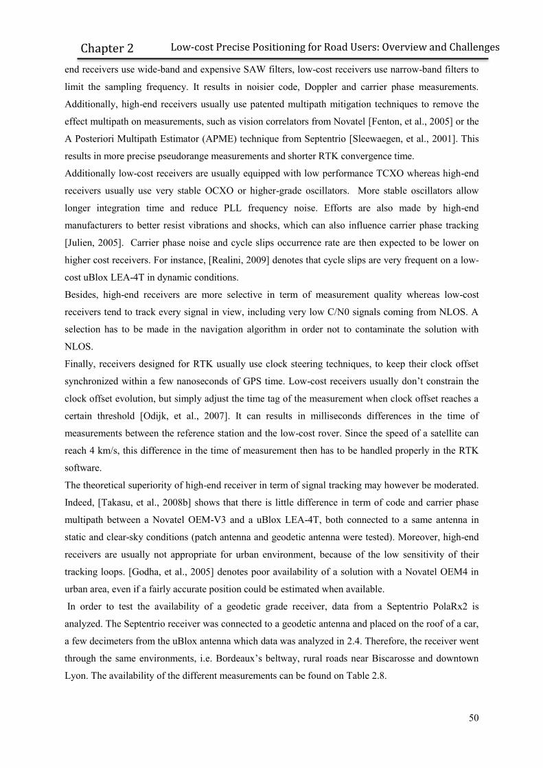
50
Low-cost Precise Positioning for Road Users: Overview and Challenges
Chapter 2
end receivers use wide-band and expensive SAW filters, low-cost receivers use narrow-band filters to
limit the sampling frequency. It results in noisier code, Doppler and carrier phase measurements.
Additionally, high-end receivers usually use patented multipath mitigation techniques to remove the
effect multipath on measurements, such as vision correlators from Novatel [Fenton, et al., 2005] or the
A Posteriori Multipath Estimator (APME) technique from Septentrio [Sleewaegen, et al., 2001]. This
results in more precise pseudorange measurements and shorter RTK convergence time.
Additionally low-cost receivers are usually equipped with low performance TCXO whereas high-end
receivers usually use very stable OCXO or higher-grade oscillators. More stable oscillators allow
longer integration time and reduce PLL frequency noise. Efforts are also made by high-end
manufacturers to better resist vibrations and shocks, which can also influence carrier phase tracking
[Julien, 2005]. Carrier phase noise and cycle slips occurrence rate are then expected to be lower on
higher cost receivers. For instance, [Realini, 2009] denotes that cycle slips are very frequent on a low-
cost uBlox LEA-4T in dynamic conditions.
Besides, high-end receivers are more selective in term of measurement quality whereas low-cost
receivers tend to track every signal in view, including very low C/N0 signals coming from NLOS. A
selection has to be made in the navigation algorithm in order not to contaminate the solution with
NLOS.
Finally, receivers designed for RTK usually use clock steering techniques, to keep their clock offset
synchronized within a few nanoseconds of GPS time. Low-cost receivers usually don’t constrain the
clock offset evolution, but simply adjust the time tag of the measurement when clock offset reaches a
certain threshold [Odijk, et al., 2007]. It can results in milliseconds differences in the time of
measurements between the reference station and the low-cost rover. Since the speed of a satellite can
reach 4 km/s, this difference in the time of measurement then has to be handled properly in the RTK
software.
The theoretical superiority of high-end receiver in term of signal tracking may however be moderated.
Indeed, [Takasu, et al., 2008b] shows that there is little difference in term of code and carrier phase
multipath between a Novatel OEM-V3 and a uBlox LEA-4T, both connected to a same antenna in
static and clear-sky conditions (patch antenna and geodetic antenna were tested). Moreover, high-end
receivers are usually not appropriate for urban environment, because of the low sensitivity of their
tracking loops. [Godha, et al., 2005] denotes poor availability of a solution with a Novatel OEM4 in
urban area, even if a fairly accurate position could be estimated when available.
In order to test the availability of a geodetic grade receiver, data from a Septentrio PolaRx2 is
analyzed. The Septentrio receiver was connected to a geodetic antenna and placed on the roof of a car,
a few decimeters from the uBlox antenna which data was analyzed in 2.4. Therefore, the receiver went
through the same environments, i.e. Bordeaux’s beltway, rural roads near Biscarosse and downtown
Lyon. The availability of the different measurements can be found on Table 2.8.

51
Low-cost Precise Positioning for Road Users: Overview and Challenges
Chapter 2
Table 2.8 Number of tracked satellites statistics for each measurement for a Septentrio PolaRx2+geodetic
antenna in different environments
Forest roads Bordeaux's beltway Lyon's downtown
Visible satellites C1 D1 L1 C1 D1 L1 C1 D1 L1
at least 4 satellites
93.9% 91.7% 83.6% 99.6% 97.0% 89.7% 97.1% 95.2% 89.8%
at least 5 satellites
89.3% 86.1% 77.6% 99.2% 95.9% 87.9% 91.8% 88.7% 80.4%
at least 6 satellites
83.2% 79.1% 69.2% 98.4% 94.4% 84.8% 83.4% 79.2% 69.0%
at least 7 satellites
75.7% 71.4% 61.2% 96.9% 91.8% 80.5% 68.0% 62.8% 52.1%
at least 8 satellites
67.5% 62.8% 53.1% 93.2% 87.0% 73.1% 49.7% 44.6% 35.0%
In comparison with Table 2.2, measurements are significantly less available than for the uBlox
receiver. In particular, 8 carrier phase measurements are visible only 53.1% of the time on forest roads
and only 35.0% of the time in downtown Lyon, whereas it was 76.5% and 61.6% in the case of the
uBlox receiver. It can be denoted that at least 5 code measurements are available 89.3% of the time in
forest roads, whereas this percentage reaches 91.8% in urban environment. It can be due to complete
signal maskings that are more frequent on rural roads than in the studied urban environment, probably
due to tree foliage. On the other hand partial signal maskings tend to make the availability of more
than 7 satellites less important in urban environment than on rural roads with the PolaRx2 receiver.
2.5.2.2 Specific Case of GLONASS Code Measurements
As seen in 2.2.2.2, GLONASS FDMA structure implies that code measurements can be offset by
inter-channel biases. In the case of high-end receivers, specific care is taken by the manufacturers in
order to calibrate these biases.
To illustrate this, 3 baselines are considered:
a baseline between a NVS08C plus Tallysman Wireless patch antenna and a Trimble receiver
(TLSE from IGS station),
a baseline between a Leica receiver (TLIA from RGP station) and a Trimble receiver (TLSE)
a baseline between a Trimble receiver (CSTN from RGP station) and a Trimble receiver
(TLSE).
Baselines are approximately 500 meters, 500 meters and 4 kms long and were surveyed in advance
using a post-processing RTK software. Observation lasted 2 days from June 22nd to June 23rd, 2012,
with 30 second sample rate.

52
Low-cost Precise Positioning for Road Users: Overview and Challenges
Chapter 2
Code inter-channel biases were isolated by double-differencing code measurements using only
satellites with a null GLONASS frequency number as reference satellite (PRN 11 and PRN 15 at this
time). Epochs when PRN 11 or PRN 15 were not visible were discarded. Then, double-differenced
geometric range is removed using broadcast ephemeris and a-priori known coordinates of antennas L1
phase centers. GLONASS code inter-channel bias were then estimated as constant biases.
Figure 2.11 shows estimated GLONASS code inter-channel bias difference between the 3 baselines as
a function of the GLONASS frequency number.
Figure 2.11 Averaged GLONASS code double-differenced inter-channel biases. Data was collected over 2 days.
Only satellites with a null GLONASS frequency number were chosen as reference satellite.
It can be seen that code inter-channel biases are not negligible in both heterogeneous baseline cases.
However they are clearly linear with frequency in the case of a baseline between 2 geodetic receivers
and antennas, while their dependence with frequency seems more chaotic in the case of the baseline
including the NVS-08C. If not properly handled, these biases reduce the quality of differential
GLONASS pseudoranges and degrade the position and float ambiguities estimation.
The advantage of the code inter-channel bias linearity with frequency found between geodetic
receivers is that the slope is easily estimable as a unique additional parameter using the entire
GLONASS geometry, instead of estimating separate biases for each frequency as in [Kozlov, et al.,
2000].
Additionally, these code biases don’t seem to be identical from one NVS receiver to the other. On
Figure 2.13, two NVS-08C receivers with same firmware v02.04 were connected to the same patch
antenna via a splitter and code measurements from each receiver were differenced with TLSE
(Trimble receiver). A picture of the 2 receivers can be found on Figure 2.12.
-8 -6 -4 -2 0 2 4 6-3
-2
-1
0
1
2
3
4
5
6
7Averaged Glonass Code Double-differenced Inter-channel bias as a funtion of frequency
GLONASS Frequency Number
mete
rs
NVS08C-Trimble baseline
Leica-Trimble baseline
Trimble-Trimble baseline

53
Low-cost Precise Positioning for Road Users: Overview and Challenges
Chapter 2
Figure 2.12 Picture of the 2 tested NVS-08C receivers. NVS-08C n°1 is on the left.
As seen on Figure 2.12, the 2 receivers didn’t have the same hardware number on the top of the chip,
although the firmware was strictly identical.
Inter-channel biases were then isolated using the same method as previously. Data was collected
during one day (March 29th, 2012) with 30s samples and a baseline was formed with TLSE (Trimble
receiver). As seen on Figure 2.13, a clear discrepancy can be seen between biases from the 2 receivers.
Although this test was performed on only 2 receivers, a global calibration for any NVS-08C doesn’t
seem to be possible.

54
Low-cost Precise Positioning for Road Users: Overview and Challenges
Chapter 2
Figure 2.13 Averaged code GLONASS double-differenced inter-channel bias, for 2 distinct NVS08C connected to
the same antenna. Double-differences are formed with TLSE (Trimble receiver) observations for both receivers.
NVS08C n°1 will be used in the rest of this work for practical reasons as contrary to NVS08C n°2, it
was equipped with a back-up battery.
2.5.2.3 Specific Case of GLONASS Carrier Phase Measurements
-8 -6 -4 -2 0 2 4 6-2
-1
0
1
2
3
4
5
6
7Averaged Glonass Code Double-differenced Inter-channel bias as a funtion of frequency
GLONASS Frequency Number
mete
rs
NVS08C n°1-Trimble baseline
NVS08C n°2-Trimble baseline

55
Low-cost Precise Positioning for Road Users: Overview and Challenges
Chapter 2
Double-differenced GLONASS carrier phase measurements can also be offset by inter-channel biases,
as indicated in equation (2.19). In order to isolate GLONASS carrier phase residuals, data from the 2
NVS receivers are double-differenced and a zero baseline is formed. Additional ambiguity is first
isolated by subtracting single-differenced code measurements from single-differenced carrier phase
measurements, and then removed from double-differenced carrier phase as explained in 2.2.2.2. Once
again, only satellites with a null frequency number were chosen as reference. Results can be found on
Figure 2.14.
Figure 2.14 Double-differenced carrier phase residual after removing additional ambiguity between 2 NVS08C
receiver with similar firmware. Only epochs with a null frequency number reference satellite are considered.
It can be seen that double-differenced carrier phase residuals are biased, despite the fact the 2 receiver
had similar firmware. Biased double-differenced carrier phase residuals prevent from a reliable
GLONASS integer ambiguity resolution.
2.5.3 Differences Between a Low-cost Patch Antenna and a
Geodetic Antenna
2.5.3.1 General discussion
2.5.3.2 Phase Center Offset Estimation of the TW2410
In order to determine if the phase center position of the TW2410 used in this PhD study coincides with
its physical center, data was collected on October 30th, 2012. A point on a car was surveyed using a
0 500 1000 1500 2000 2500 3000-0.02
-0.015
-0.01
-0.005
0
0.005
0.01
0.015
0.02Double differenced GLONASS carrier phase residuals
Epochs (30s)
mete
rs
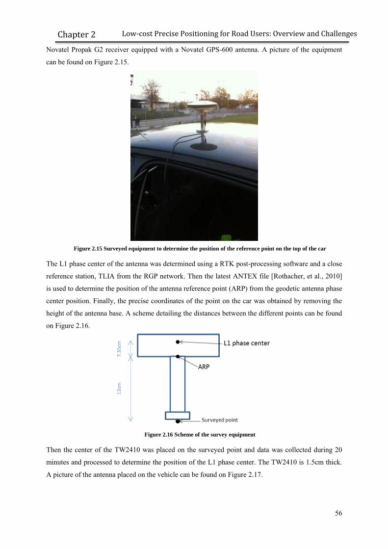
56
Low-cost Precise Positioning for Road Users: Overview and Challenges
Chapter 2
Novatel Propak G2 receiver equipped with a Novatel GPS-600 antenna. A picture of the equipment
can be found on Figure 2.15.
Figure 2.15 Surveyed equipment to determine the position of the reference point on the top of the car
The L1 phase center of the antenna was determined using a RTK post-processing software and a close
reference station, TLIA from the RGP network. Then the latest ANTEX file [Rothacher, et al., 2010]
is used to determine the position of the antenna reference point (ARP) from the geodetic antenna phase
center position. Finally, the precise coordinates of the point on the car was obtained by removing the
height of the antenna base. A scheme detailing the distances between the different points can be found
on Figure 2.16.
Figure 2.16 Scheme of the survey equipment
Then the center of the TW2410 was placed on the surveyed point and data was collected during 20
minutes and processed to determine the position of the L1 phase center. The TW2410 is 1.5cm thick.
A picture of the antenna placed on the vehicle can be found on Figure 2.17.

57
Low-cost Precise Positioning for Road Users: Overview and Challenges
Chapter 2
Figure 2.17 Patch antenna sticked to the roof of the car on the surveyed reference point
The difference between the surveyed coordinates and the L1 phase center is reported on Table 2.9. Table 2.9 Difference between the L1 phase center of the TW2410 GPS/GLONASS antenna and the surveyed
coordinates. The antenna is 1.5 cm thick.
North East Up
Difference between L1 phase
center and surveyed point
0.5 centimeter 0.1 centimeter 1.35 centimeter
As seen on the table, the phase center of the TW2410 antenna in these conditions corresponds very
well to the physical center on the top of the antenna, which is 1.5 centimeter above the surveyed point.
2.5.3.3 Impact of the Ground Plane
In order to determine the impact of the placement of the antenna on the vehicle, a second data
collection of 20 minutes was performed immediately after the previous one, so that satellite geometry
and atmospheric effect can be considered similar. However, the antenna was placed on top of the
antenna stand this time, centered on the same surveyed point. A picture of the roof of the car can be
found on Figure 2.18.

58
Low-cost Precise Positioning for Road Users: Overview and Challenges
Chapter 2
Figure 2.18 Picture of the TW2410 antenna, no longer sticked to the roof of the car.
In these conditions, the roof of the car no longer directly acts as a ground plane for the antenna. Data
collected is then compared to the data set where the antenna was sticked to the roof of the car.
Different statistics are analyzed:
Average C/N0 value. The average value of all tracked satellite is compared in the 2 data sets.
Antenna L1 phase center position relative to the center of the top of the antenna
Standard deviation of ambiguity-fixed position in North, East and Up coordinates. The
ambiguity was fixed in post-processing and position was estimated using unambiguous GPS
and GLONASS carrier phase measurements.
Results can be found on Table 2.10. Table 2.10 Average C/N0, Phase center offset and carrier phase standard deviation depending on the placement
of the TW2410 antenna
Average C/N0
Phase center offset Fixed-position standard
deviation
North (cm)
East (cm)
Up (cm)
North (cm)
East (cm)
Up (cm)
Antenna sticked to the roof
43.1 dB.Hz 0.5 0.1 -0.2 0.2 0.2 0.2
Antenna placed on a stand
40.6 dB.Hz 0.2 0.4 -5.5 0.4 0.2 0.4
It can be seen that the placement of the antenna on the car has a great effect on measurements
characteristics. The average C/N0 is decreased by 2.5dB when the antenna is not placed directly on the

59
Low-cost Precise Positioning for Road Users: Overview and Challenges
Chapter 2
roof. Moreover, the phase center of the antenna is moved down by about 5.5 centimeters. Finally, the
standard deviation of carrier phase measurements is almost doubled.
These changes in measurements characteristics come from the combined effect of:
the strong multipath signals coming from the vehicle metallic roof in the case the antenna is
placed on a stand
the actual variation of the antenna characteristics due to the different ground planes.
Therefore, very special care has to be taken in the placement of the antenna on the vehicle.
2.5.4 Conclusions on the Possibility of Applying RTK Algorithm on
a Low-cost System
In this sub-chapter, the main differences between a low-cost receiver and a high-end receiver and
between a low-cost patch antenna and a geodetic antenna in term of L1 measurement characteristics
have been described. Low-cost receivers were shown to have a lower quality of measurement but a
higher sensitivity. In particular, GLONASS code and carrier phase measurements have been shown to
be affected by uncalibrated biases on the tested receiver. These biases prevent from fully benefitting of
the additional constellation as they will bias the float ambiguity solution and prevent GLONASS
integer ambiguity resolution.
Additionally it was underlined that antenna greatly influence the quality of both code and carrier phase
measurements. In particular, the placement of the patch antenna on a large metallic ground plane was
shown to bring benefit to phase center position stability and carrier phase standard deviation in our
test. In the presented configuration, the phase center position of the studied patch antenna was
measured and coincides with the physical center of the antenna, provided the antenna is sticked to the
roof of the car. If it is not the case, variations of the phase center position were found to be essentially
in the up direction.
2.6 Architecture of the Proposed Solution
2.6.1 Road User Low-cost Precise Positioning Challenges
Although very difficult to define because of its diversity, road user environment can be generally
considered as a non-friendly environment for satellite navigation. Signal attenuation from trees, high-
power reflection from buildings or reduced line-of-sight signal availability degrades the tracking
continuity and measurements quality, as seen in 2.4. Moreover, the effect of the environment on
measurements quality will be amplified by the fact that low-cost elements are used, notably a patch
antenna. Multipath rejection will be low while cycle slips occurrence frequency can be potentially
high, especially in dynamic conditions. Besides, GLONASS code and carrier phase measurements are
heavily biased, making them almost useless for ambiguity resolution without additional calibration as

60
Low-cost Precise Positioning for Road Users: Overview and Challenges
Chapter 2
shown in 2.5.2. Moreover, issues such as time synchronization between the rover and the reference
station, large phase center position variation and communication link outages might degrade even
further the accuracy of the final position.
Different solutions have been proposed to apply RTK techniques to difficult environment and/or low-
cost receivers. In general, single-epoch ambiguity resolution, i.e. initialization of ambiguity vector at
each epoch is recommended as in [Kubo, 2009] or [Bahrami, et al., 2010]. Single-epoch ambiguity
resolution allows avoiding the issue related to cycle slips, which can be very frequent in low-cost
receivers. However, instantaneous ambiguity resolution requires very precise code measurements or
estimated position and is suboptimal as the constant nature of the ambiguity value from one epoch to
the other is not taken into account in the Kalman filter transition matrix. Indeed, cycle slips usually
don’t occur at every epoch on every satellite. In order to quicken the time to fix ambiguity, Doppler
measurements are used to smooth pseudoranges [Bahrami, et al., 2010] or reduce the ambiguity search
space [Kubo, 2009]. Altitude-aiding can also be used for the same purpose [Kubo, et al., 2007].
Hybridization with inertial sensor is also proposed to cope with the problem of cycle slips and allow
continuous estimation [Takasu, et al., 2008].
Low-cost receivers are also used in [Realini, 2009] to provide a carrier smoothed DGPS solution.
However no ambiguity resolution is applied, which limits the final solution accuracy. Ambiguity
resolution with low-cost receiver is proposed in the software RTKLIB [Takasu, et al., 2009]. RTKLIB
is a set of open-source software, notably allowing RTK and PPP processing in both real-time and post-
processing mode. However, the performance of RTKLIB in difficult environments with kinematic
conditions remains unclear. Finally, [Odijk, et al., 2007] proposes a method based on a time-difference
approach. However, it can only be applied for a limited period, as the accuracy slowly degrades with
time.
In order to cope with both the environment and the low-cost constraint, a precise positioning software
architecture is proposed and generally described in the next section. Detailed specificities of each
software block, as well as tests based on real data collection will be depicted in the next chapters.
2.6.2 Proposed Precise Positioning algorithm
Different choices were made to cope with the issues related to low-cost precise positioning in difficult
environments. The first one was the choice of RTK over PPP, as explained in 2.4.9. Both GPS and
GLONASS satellite measurements will be used to improve availability in urban environments. Galileo
satellite navigation data was not available at the time this manuscript was written and therefore Galileo
satellites could not be used. Single-frequency measurements on L1 will be used, in order to meet the
cost constraint. As explained in 0, the NVS-08C receiver GPS/GLONASS measurements are used,
connected to a TW2410 patch antenna.
Concerning the software, the designed navigation filter is composed of 2 modules: a pre-processing
module and a PVT module.

61
Low-cost Precise Positioning for Road Users: Overview and Challenges
Chapter 2
In the pre-processing module, described in chapter 3, a measurement selection is made using both
C/N0 masks and a multipath detection algorithm to reject NLOS and multipath-contaminated
measurements. GLONASS code measurements are also corrected of inter-channel biases. Moreover, a
cycle slip resolution technique is also performed, to allow a continuous estimation of carrier phase
ambiguities. This approach differs from classic urban RTK procedure based on single-epoch
ambiguity resolution, in which only dynamic and Doppler measurements are used to smooth
trajectory. The preprocessing module also determines the appropriate weight associated to each
measurement. Indeed measurements have to be weighted as closely as possible from their actual error
to optimize the estimation. In particular a new Doppler weighting scheme is introduced, function of
both velocity and C/N0, as Doppler measurement multipath error has been shown to be highly
correlated with antenna speed in section 2.4.3. An environment-dependent pseudorange weighting
scheme is introduced in the third chapter.
Secondly, a Kalman filter, described in chapter 4, is used to precisely estimate position among other
parameters. The specificity of road user dynamic is taken into account by applying a vertical velocity
constraint. GLONASS carrier phase measurements are calibrated, in order to be able to estimate both
GPS and GLONASS ambiguities as integers and fully benefit from the GLONASS constellation. GPS
and GLONASS carrier phase ambiguities are estimated as integers using the LAMBDA method. This
choice was made because of:
the performance of the method, as it was proven to maximize the probability that the correct
integer vector is found [Teunissen P. , 1999]
the easiness of implementation, as LAMBDA Matlab® code is freely distributed by the
University of Delft.
In order to cope with a potential loss of the communication link, a seamless switch from RTK to PPP
by initializing PPP filter with RTK ambiguities will be introduced. This technique allows keeping a
higher level of accuracy instead of switching to single-point positioning.
A scheme of the proposed solution architecture can be found on Figure 2.19.

62
Low-cost Precise Positioning for Road Users: Overview and Challenges
Chapter 2
Figure 2.19 General scheme of the proposed solution

63
Pre-processing Module Description
Chapter 3
Chapter 3. Pre-processing Module Description
The pre-processing module has 3 purposes:
To remove degraded measurements by applying an a-priori mask
To detect and exclude remaining multipath-contaminated measurements
To detect and repair cycle slips in order to continuously smooth pseudoranges with carrier
phase measurements.
These operations are performed routinely, before estimating the baseline vector and other parameters
in the Kalman filter. The point is to use the “cleanest” measurements in the Kalman filter in order to
avoid biasing or degrading the solution quality. The different steps of the pre-processing module will
be described in the next sections.
3.1 Reducing the Impact of Multipath and Inter-channel
Biases on Measurements by Appropriate Masking and
Weighting
It has been shown in Chapter 2 that the availability of measurements of a low-cost receiver such as the
uBlox LEA-4T was good in most environments encountered by road users. However, some
measurements were heavily affected by multipath, and pseudorange error could reach dozens of
meters. If these measurements are not appropriately down-weighted or removed, errors can be
propagated in the position solution during multiple epochs. The proposed solution uses a detection and
exclusion module, which will be presented in section 3.2. This type of Fault Detection and Exclusion
(FDE) algorithm are subject to erroneous rejection of good measurements especially in the case of
large or multiple biases [Kuusniemi, 2005]. Therefore, an initial selection of measurements using a-
priori criteria is necessary.
Two main criterions can be generally used to select an observation: the C/N0 value as provided by the
receiver and the satellite elevation. To determine which criterion is the most relevant, [Kuusniemi,
2005] analyses code and Doppler residuals in different environments. Even if larger code and Doppler

64
Pre-processing Module Description
Chapter 3
multipath error were obtained for low-elevation satellite, a stronger correlation with estimated C/N0
value was demonstrated. This correlation will be studied in the next section using real data analysis
from road user environments. This real data analysis should have been performed with the targeted
receiver, i.e. the NVS-08C equipped with a TW2410 antenna. However, no large data set collected on
road environments with this receiver and antenna was available at the time this analysis was
performed. Therefore, the correlation between code multipath error and C/N0 value, and Doppler
multipath error and C/N0 value was performed using the measurement campaign described in section
2.4.2. It is then based on a uBlox LEA-4T receiver equipped with an ANN-MS patch antenna.
However, considering the NVS-08C and the uBlox LEA-4T are both low-power and high sensitivity
receiver, their measurement quality is expected to be similar.
3.1.1 Weighting and Masking Code Measurements
3.1.1.1 Data Analysis
In order to determine the appropriate mask value and weighting scheme for pseudoranges, real data
from the data set presented in 2.4.2 has been analyzed. It can be denoted that this data set was
collected before the commercial release of the targeted receiver NVS-08C, and was then using a uBlox
LEA-4T. Again, double-differenced code multipath from a rural road, Bordeaux’s beltway and
downtown Lyon are isolated. The reference satellite used to form double differences was chosen as the
one with the highest C/N0. Each multipath error is then associated to the C/N0 value of the secondary
satellite. Standard deviation and mean code error value are plotted on Figure 3.1 and Figure 3.2.
Figure 3.1 Standard deviation of code measurement error as a
function of C/N0, in the different environments considered, using a
uBlox LEA-4T + patch antenna
Figure 3.2 Mean of code measurement error as a function
of C/N0, in the different environments considered, using a
uBlox LEA-4T + patch antenna
It can clearly be seen that the standard deviation of double-differenced code measurements as a
function of C/N0 value depends on the environment considered. In urban environment, a clear increase
of the standard deviation from 40dB.Hz to 30dB.Hz exists. This trend is also visible for mean code
30 35 40 45 50 550
5
10
15
20
25Code Standard deviation as a function of CN0
CN0 (dB.Hz)
mete
rs
Rural roads
Bordeaux's beltway
Downtown Lyon
30 35 40 45 50 55-2
0
2
4
6
8
10
12
14
16Code mean error value as a function of CN0
CN0 (dB.Hz)
mete
rs
Rural roads
Bordeaux's beltway
Downtown Lyon
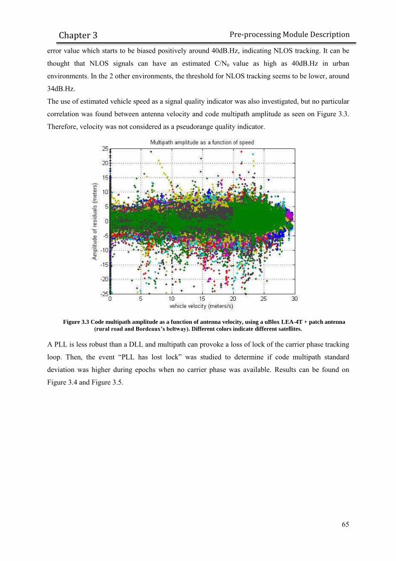
65
Pre-processing Module Description
Chapter 3
error value which starts to be biased positively around 40dB.Hz, indicating NLOS tracking. It can be
thought that NLOS signals can have an estimated C/N0 value as high as 40dB.Hz in urban
environments. In the 2 other environments, the threshold for NLOS tracking seems to be lower, around
34dB.Hz.
The use of estimated vehicle speed as a signal quality indicator was also investigated, but no particular
correlation was found between antenna velocity and code multipath amplitude as seen on Figure 3.3.
Therefore, velocity was not considered as a pseudorange quality indicator.
Figure 3.3 Code multipath amplitude as a function of antenna velocity, using a uBlox LEA-4T + patch antenna
(rural road and Bordeaux’s beltway). Different colors indicate different satellites.
A PLL is less robust than a DLL and multipath can provoke a loss of lock of the carrier phase tracking
loop. Then, the event “PLL has lost lock” was studied to determine if code multipath standard
deviation was higher during epochs when no carrier phase was available. Results can be found on
Figure 3.4 and Figure 3.5.

66
Pre-processing Module Description
Chapter 3
Figure 3.4 Code standard deviation in different environments
with a uBlox and a patch antenna, selecting only epochs when PLL
is locked
Figure 3.5 Code standard deviation in different
environments with a uBlox and a patch antenna, selecting
only epochs when PLL has lost lock
It can be seen that code standard deviation evolution as a function of C/N0 are almost similar in each
case. Then the event “PLL has lost lock” was not retained as a code quality indicator.
Figure 3.1 and Figure 3.2 underline the difficulty to determine an appropriate weighting scheme
function of C/N0 that would fit any type of environment. A solution is to use an environment-
dependent weighting scheme in order to separate the rural/suburban case from the urban environment.
3.1.1.2 Proposed Weighting Schemes
As stated earlier, weighting all pseudoranges with the same weight in the positioning filter is in
general not optimal [Kuusniemi, 2005]. Different weighting schemes have been proposed in the
literature. Some use the mapping function existing between the noise variance and the C/N0 value
[Langley, 1997]. However, the internal receiver parameters required are usually not available to the
user [Bisnath, et al., 2001]. Additionally as multipath error can be significantly higher than the noise
error, the formula may be overly optimistic in the case of a multipath-contaminated environment.
[Realini, 2009] proposes a weighting scheme based on both C/N0 and elevation, and adapted to uBlox
LEA-4T measurements. However, the proposed empirical model was determined using only static
measurements which may not reflect the actual multipath error encountered by a road user. A model
was proposed in [Kuusniemi, 2005] specifically for difficult environments based on the function:
with the C/N0 value in dB.Hz, the variance of code measurements and and empirical
parameters. This last model suits very well the estimated standard deviation in rural environment and
on Bordeaux’s beltway using coefficient and , as seen on Figure 3.6.
30 35 40 45 50 550
5
10
15
20
25Code Standard deviation as a function of CN0 when PLL is locked
CN0 (dB.Hz)
mete
rs
Rural roads
Bordeaux's beltway
Downtown Lyon
30 35 40 45 50 550
5
10
15
20
25Code Standard deviation as a function of CN0 when PLL tracking is lost
CN0 (dB.Hz)
mete
rs
Rural roads
Bordeaux's beltway
Downtown Lyon

67
Pre-processing Module Description
Chapter 3
Figure 3.6 Estimated standard deviation in the
different studied environments and model proposed in
[Kuusniemi, 2005] with and
Figure 3.7 Estimated standard deviation in downtown
Lyon and model proposed in [Kuusniemi, 2005] with
and
However, the model proposed for rural and beltway environment doesn’t capture the change in the
trend of the standard deviation when NLOS starts to get tracked in downtown Lyon. Therefore, a
different model is used for urban environment. Coefficient and were selected for
urban environment, since this model was shown to fit relatively well the estimated pseudorange
standard deviation, as seen on Figure 3.7.
Using a model that fits estimated standard deviation in urban environment may not be the optimal
solution in term of final position accuracy. Indeed, a multipath detection and rejection technique will
be introduced in 3.2. It is intended to discard measurements heavily contaminated by multipath, in
particular NLOS tracking. Then as the urban data set was analyzed without this module, the estimated
standard deviation may be overly pessimistic for the positioning module but too optimistic to weight
measurements in the multipath rejection algorithm.
However, a unique weighting model for pseudoranges was chosen in both the multipath rejection
algorithm and the positioning filter for sake of simplicity.
3.1.1.3 Discussion on C/N0 Mask Value
The determination of an a-priori C/N0 mask value is a very difficult task since the final quality of
position depends on both the satellite geometry and the measurements accuracy. Then, masking low
C/N0 satellites might improve the expected measurement accuracy, but degrade satellite geometry. In
order to illustrate this, the average PDOP and the availability of the position, i.e. the percentage of
epochs with at least 4 pseudoranges, are plotted on Figure 3.8 and Figure 3.9. As expected, the higher
the C/N0 mask value, the lower the quality of the satellite geometry and the availability. Therefore, the
optimal C/N0 mask value is a trade-off between geometry strength and expected measurement quality.
30 35 40 45 50 550
1
2
3
4
5
6
7
8
9
10
CN0 (dB.Hz)
mete
rs
Estimated standard deviation and proposed model for peri-urban and rural roads environments
Rural roads
Bordeaux's beltway
Downtown Lyon
a=1, b=281²
30 35 40 45 50 550
5
10
15
20
25
CN0 (dB.Hz)
mete
rs
Estimated standard deviation and proposed model for urban environments
Downtown Lyon
a=-1.5, b=731²
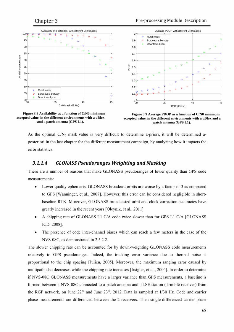
68
Pre-processing Module Description
Chapter 3
Figure 3.8 Availability as a function of C/N0 minimum
accepted value, in the different environments with a uBlox
and a patch antenna (GPS L1).
Figure 3.9 Average PDOP as a function of C/N0 minimum
accepted value, in the different environments with a uBlox and a
patch antenna (GPS L1).
As the optimal C/N0 mask value is very difficult to determine a-priori, it will be determined a-
posteriori in the last chapter for the different measurement campaign, by analyzing how it impacts the
error statistics.
3.1.1.4 GLONASS Pseudoranges Weighting and Masking
There are a number of reasons that make GLONASS pseudoranges of lower quality than GPS code
measurements:
Lower quality ephemeris. GLONASS broadcast orbits are worse by a factor of 3 as compared
to GPS [Wanninger, et al., 2007]. However, this error can be considered negligible in short-
baseline RTK. Moreover, GLONASS broadcasted orbit and clock correction accuracies have
greatly increased in the recent years [Oleynik, et al., 2011]
A chipping rate of GLONASS L1 C/A code twice slower than for GPS L1 C/A [GLONASS
ICD, 2008].
The presence of code inter-channel biases which can reach a few meters in the case of the
NVS-08C, as demonstrated in 2.5.2.2.
The slower chipping rate can be accounted for by down-weighting GLONASS code measurements
relatively to GPS pseudoranges. Indeed, the tracking error variance due to thermal noise is
proportional to the chip spacing [Julien, 2005]. Moreover, the maximum ranging error caused by
multipath also decreases while the chipping rate increases [Irsigler, et al., 2004]. In order to determine
if NVS-08C GLONASS measurements have a larger variance than GPS measurements, a baseline is
formed between a NVS-08C connected to a patch antenna and TLSE station (Trimble receiver) from
the RGP network, on June 22nd and June 23rd, 2012. Data is sampled at 1/30 Hz. Code and carrier
phase measurements are differenced between the 2 receivers. Then single-differenced carrier phase
30 35 40 4550
55
60
65
70
75
80
85
90
95
100Availavility (>3 satellites) with different CN0 masks
CN0 Mask(dB.Hz)
Avaib
ility
perc
enta
ge
Rural roads
Bordeaux's beltway
Downtown Lyon
30 35 40 451
1.1
1.2
1.3
1.4
1.5
1.6
1.7
1.8
1.9
2Average PDOP with different CN0 masks
CN0 (dB.Hz)
PD
OP
Rural roads
Bordeaux's beltway
Downtown Lyon

69
Pre-processing Module Description
Chapter 3
measurements are subtracted from single-differenced code measurements. The mean of this so-called
“code-minus-carrier” observable is removed. Finally standard deviations of GPS and GLONASS
measurements are estimated from this zero-mean observable. Results can be found on Table 3.1. Table 3.1 Estimated standard deviation of GPS and GLONASS double-differenced code measurements, from
static data collection performed on June 22nd and June 23rd, 212 between a NVS-08C and Trimble receiver
GPS code measurements GLONASS code measurements
Standard deviation 0.89 meters 1.17 meters
According to these measurements, GLONASS code observation associated variance should be down-
weighted by a factor of approximately 1.3 relative to GPS code observation variance.
Lastly, code inter-channel biases can be corrected using 2 techniques:
Remove inter-channel biases using a-priori estimated value stored in a table. It was shown on
Figure 2.11 and Figure 2.13 that inter-channel biases were almost similar at 2 months interval.
Dependence on time and temperature should however be investigated. This solution can also
be easily implemented by changing the GLONASS code biases correction inside the chip, via
message A0h of the BINR protocol [NVS Technologies AG., 2012].
Estimate a separate bias for each channel in the navigation software, as in [Kozlov, et al.,
2000].
However, each method has drawbacks. The first requires a calibration of potentially each NVS-08C
before using it, as the inter-channel bias was found to be different on 2 similar receivers, i.e. with the
same firmware, connected to the same antenna.
The second adds additional parameters to estimate and is sensitive to code multipath error. Indeed, any
bias in code pseudorange will be lumped into the code inter-channel bias estimate.
Therefore, the first method will be used and code inter-channel biases will be corrected using a-priori
values estimated in a clear-sky environment. In particular, values estimated in 2.5.2.2 and plotted on
Figure 2.13 will be used to correct NVS receiver pseudoranges used in this thesis.
However, it is important to note that these biases only correct NVS-08C code measurements relative to
the high-end receiver brand used during the calibration process. A bias will still exist if a receiver from
a different brand is used as reference station. Therefore, applying a code inter-channel correction does
not prevent from estimating code inter-channel biases in the RTK Kalman filter. To do so, the NVS-
08C code inter-channel biases can be estimated as a linear function of the GLONASS frequency
number in that case.
3.1.2 Weighting and Masking of Doppler Measurements
3.1.2.1 Data Analysis

70
Pre-processing Module Description
Chapter 3
Doppler measurements are relatively difficult to weight. Indeed, [Aminian, 2011] underlines that
multipath effect on Doppler measurements depends on both signal-to-noise ratio and velocity. In a
static environment, the influence of multipath signals on Doppler measurements is null, as the
frequency of the reflected signals and the direct signal are equal. Then measurements can be weighted
using FLL tracking loop jitter due to thermal noise, as in [Kubo, 2009] or [Aminian, 2011]. However
this weighting would be overly optimistic in the case of a moving antenna. Indeed Doppler
measurement error was shown to be heavily correlated with receiver speed on Figure 2.7. In order to
determine a link between vehicle speed and multipath amplitude, multipath residuals were plotted as a
function of the vehicle velocity norm. Results can be found on Figure 3.10 , using data from the 3
studied environments.
Figure 3.10 Doppler measurement error as a function of vehicle reference speed, using data from the 3 studied
environments and a uBlox LEA-4T + patch antenna
Doppler multipath tends to increase with the vehicle speed until around 15m/s, and decrease after this.
An interpretation is that the vehicle speed increases the frequency offset of the multipath. If the speed
of the variation of the phase (or frequency) of the multipath exceeds the PLL (or FLL) bandwidth, the
multipath effects on tracking starts to be filtered out. In the case of the high-end receiver, Doppler
multipath is heavily reduced and seems relatively stable with speed.
In order to determine the influence of both speed and C/N0 on Doppler measurements, the standard
deviation of the Doppler measurements was estimated as a function of the vehicle speed and C/N0, as
seen on Figure 3.11. A trend is clearly visible, for both velocity and C/N0. Then both parameters can
be used as a measurement quality indicator.

71
Pre-processing Module Description
Chapter 3
Figure 3.11 Doppler measurements error as a function of vehicle reference speed and C/N0, using data from the 3
studied environments and a uBlox LEA-4T + patch antenna
3.1.2.2 Proposed Doppler Weighting Scheme and Mask
In order to weight Doppler measurements using both vehicle speed and C/N0, a new weighting scheme
is proposed based on the look-up Table 3.2. Table 3.2 Table-based weighting scheme, based on estimated Doppler measurement standard deviation as a
function of velocity and C/N0, using a uBlox LEA-4T + patch antenna with data collected in the 3 studied
environments
Doppler measurements are weighted using the standard deviation value of Table 3.2. Values in the
table are derived from Figure 3.11. As GPS and GLONASS satellites have approximately the same
wavelength, identical weighting scheme is proposed for the 2 constellations.
Once again, these values were derived using measurements from a uBlox LEA-4T receiver and a
ANN-MS antenna, whereas the targeted hardware is a NVS-08C and a TW 2410 antenna. However,
0 5 10 15 20 25 300
0.5
1
1.5
2
2.5
3
3.5Doppler Standard deviation as a function of speed and CN0
velocity (meters/s)
ST
D
30-33dB.Hz
33-36dB.Hz
36-39dB.Hz
39-42dB.Hz
42-45dB.Hz
45-48dB.Hz
48-51dB.Hz
C/N0 (dB.Hz)
Vehicle speed 30-33 dB.Hz 33-36 dB.Hz 36-39 dB.Hz 39-42 dB.Hz 42-45 dB.Hz 45-48 dB.Hz 48-51 dB.Hz
0-3 m/s 0.53 m/s 0.43 m/s 0.28 m/s 0.21 m/s 0.13 m/s 0.09 m/s 0.07 m/s
3-6 m/s 2.04 m/s 1.61 m/s 1.08 m/s 0.71 m/s 0.55 m/s 0.32 m/s 0.24 m/s
6-9 m/s 2.37 m/s 2.00 m/s 1.43 m/s 0.86 m/s 0.53 m/s 0.29 m/s 0.18 m/s
9-12 m/s 3.08 m/s 2.33 m/s 1.60 m/s 1.06 m/s 0.99 m/s 0.28 m/s 0.22 m/s
12-15 m/s 2.54 m/s 1.87 m/s 1.25 m/s 0.83 m/s 0.54 m/s 0.27 m/s 0.17 m/s
15-18 m/s 1.26 m/s 1.36 m/s 1.48 m/s 0.80 m/s 0.53 m/s 0.27 m/s 0.15 m/s
18-21 m/s 1.37 m/s 1.29 m/s 0.87 m/s 0.55 m/s 0.44 m/s 0.25 m/s 0.16 m/s
21-24 m/s 1.44 m/s 1.25 m/s 1.09 m/s 0.73 m/s 0.37 m/s 0.26 m/s 0.16 m/s
24-27 m/s 1.33 m/s 0.90 m/s 0.58 m/s 0.47 m/s 0.31 m/s 0.26 m/s 0.11 m/s
27-30 m/s 1.01 m/s 0.92 m/s 0.61 m/s 0.53 m/s 0.31 m/s 0.31 m/s 0.14 m/s

72
Pre-processing Module Description
Chapter 3
considering the 2 receiver have similar cost, power and sensitivity constraints, the derived table is used
to weight NVS-08C Doppler measurements.
With regards to the a-priori C/N0 mask value, the dilemma is the same than for code pseudorange. A
tradeoff between measurement selection and geometry degradation has to be found. However, it is
difficult to decide a-priori and the choice will be made a-posteriori in Chapter 6.
3.1.1 Weighting and Masking Carrier Phase Measurements
As explained earlier, it is very difficult to isolate and study carrier phase multipath in kinematic
environments, due to the lack of a sufficiently accurate reference trajectory. Time-differenced carrier
phase multipath can be isolated using 2 close antennas, as in [Serrano, et al., 2005]. However, this
method requires a dual-antenna system.
The quality of carrier phase depends on both atmospheric delay error and carrier tracking noise error.
Residual atmospheric delay errors are larger at lower satellite elevation, i.e. lower C/N0 value.
Similarly, carrier tracking noise error increases as C/N0 value decreases [Langley, 1997]. Then a
simple weighting based on C/N0 value is proposed [Aminian, 2011]:
( ⁄ )
(3.1)
Where:
o is taken equal to 52 dB.Hz
o is the C/N0 value in dB.Hz
o is the standard deviation of the observation at the zenith.
Tests with different values of will be performed. Since the wavelength of GLONASS measurements
are very similar to GPS wavelength, GPS and GLONASS carrier phase are weighted similarly as in
[Wanninger, et al., 2007].
3.2 Detecting and Removing Multipath-contaminated
Pseudoranges and Doppler Measurements
It has been shown in 2.4.2 and 2.4.3 that code and Doppler measurements could be affected by strong
multipath errors, particularly in urban area. In particular, NLOS can cause code measurement errors of
hundreds of meters. In order to avoid this problem, a measurement selection has to be applied. A first
measurement selection is already applied through weighting and masking, as explained in the previous
sub-chapter. However, this selection is only based on a-priori mask values and it was shown that the
trade-off between satellite geometry quality and measurement quality was difficult to find. Therefore,
73
Pre-processing Module Description
Chapter 3
a second measurement selection algorithm is introduced in this paragraph, using redundancy between
measurement to detect and exclude faulty observations.
3.2.1 Fault Detection and Exclusion
Many algorithms have been developed to detect blunders, notably in civil aviation. They are based on
measurement redundancy to detect one or multiple outliers. In particular, Receiver Autonomous
Integrity Monitoring (RAIM) techniques have been proved to work well, providing fault detection or
fault detection and exclusion using receiver measurements and optional additional sensors [Salos
Andres, 2012]. However, contrary to the civil aviation case in which the main risk is a major service
failure of the GPS system, a multi-constellation low-cost receiver in urban environment can
experience multiple blunders due to NLOS tracking. Then algorithms based on the assumption of a
unique erroneous measurement cannot be used in the particular case of low-cost navigation in difficult
environment, or with potential risks of wrong detection.
It was then decided to use a data screening method to improve the accuracy and reliability of
measurements in difficult environments. Different techniques exist including observation subset
testing [Kuusniemi, 2005], the Danish method [Jørgensen, et al., 1985], Range Consensus (RANCO)
algorithm [Schroth, et al., 2008]… The Danish method was chosen and implemented to detect
multipath-contaminated code and Doppler measurements as it is simple to implement, computationally
efficient and performs very well in practical navigation applications [Kuusniemi, 2005].
3.2.2 Danish Method Description
The Danish method is an iteratively reweighted least-square that has been used in geodetic
applications for a long time [Wieser, et al., 2002]. In this technique, residuals are examined after each
iteration. If one or multiple observation residuals amplitude exceed a defined threshold, the weight
associated to the observation is reduced exponentially and the process is repeated until the solution
converges. The threshold is usually set as a multiple of the residual associated variance. For
iteration , the covariance associated to observation is set as follows [Kuusniemi, 2005]:
|
with |
√
| (3.2)
Where:
is the residual for observation after iteration
is the th element of the residual covariance matrix diagonal after the first iteration
is the a-priori variance of the observation, using the weighting schemes presented in
3.1.1.2 and 3.1.2.2 for instance.
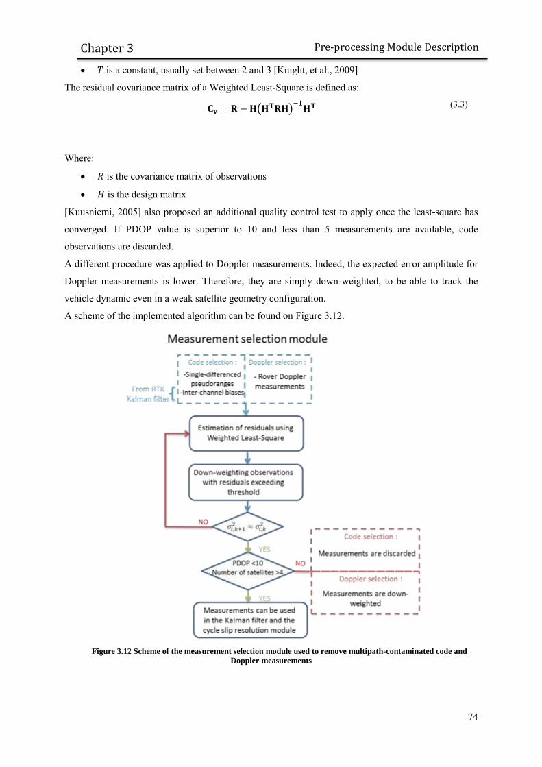
74
Pre-processing Module Description
Chapter 3
is a constant, usually set between 2 and 3 [Knight, et al., 2009]
The residual covariance matrix of a Weighted Least-Square is defined as:
( )
(3.3)
Where:
is the covariance matrix of observations
is the design matrix
[Kuusniemi, 2005] also proposed an additional quality control test to apply once the least-square has
converged. If PDOP value is superior to 10 and less than 5 measurements are available, code
observations are discarded.
A different procedure was applied to Doppler measurements. Indeed, the expected error amplitude for
Doppler measurements is lower. Therefore, they are simply down-weighted, to be able to track the
vehicle dynamic even in a weak satellite geometry configuration.
A scheme of the implemented algorithm can be found on Figure 3.12.
Figure 3.12 Scheme of the measurement selection module used to remove multipath-contaminated code and
Doppler measurements

75
Pre-processing Module Description
Chapter 3
As indicated on Figure 3.12, only single-differenced code measurements are used. Indeed, if
pseudoranges are double-differenced, an outlier in the reference satellite measurement will bias all
observations which make multipath detection more difficult. Since it was shown in 2.2.2.1 that single-
differenced or double-differenced pseudoranges could be used indifferently, pseudoranges are kept in
single-difference mode, as in [Kozlov, et al., 1997].
In the case of Doppler measurement selection, only the rover Doppler measurements were used, as
some reference stations don’t provide raw Doppler data. Measurements are weighted using weighting
schemes described in 3.1.1.2 and 3.1.2.2.
In the previous sections, methods are presented to reduce code and Doppler measurement outliers’
impact on position solution, through weighting, masking and a fault detection and exclusion algorithm.
Regarding carrier phase measurements, although they are less affected by multipath than code or
Doppler measurements, they can be offset by frequent cycle slips. If not properly detected and
estimated, cycle slips can heavily bias the final solution, as an uncontrolled error will propagate into
the position estimation. In the next section, a method is proposed for cycle slip resolution on a single-
frequency receiver.
3.3 Proposed Cycle Slip Resolution method
A cycle slip is a discontinuity of the measured carrier phase resulting from a temporary loss of lock in
the carrier tracking loop of a GNSS receiver [Kim, et al., 2002]. According to [Hofmann-Wellenhof, et
al., 1997], there are 3 causes to cycle slips: signal obstruction, low signal-to-noise ratio and failure in
the receiver software which leads to incorrect signal processing. A fourth cause pointed out by [Julien,
2005] is receiver dynamic implying a phase error within the integration time that is significantly
higher than the PLL discriminator linear domain. Although usually relatively rare in static conditions,
cycle slips occurrence can be very frequent for low-cost moving receivers [Realini, 2009]. It is then
very important to detect them and if possible to repair them in order to estimate ambiguities as
constants.
3.3.1 Real-Time Cycle Slip Detection and Resolution Techniques
Algorithms using carrier phase can solve the problem of cycle slips by:
Making no assumption on the constant value of the ambiguity. It is the basis of single-epoch
ambiguity resolution in which ambiguity vector is reinitialized at each epoch.
Detecting cycle slips and reinitializing the estimated ambiguity value when a cycle slip is
detected.
Detecting and repairing cycle slips so that the ambiguity can be assumed constant over time
even in the presence of cycle slips.

76
Pre-processing Module Description
Chapter 3
The first technique is traditionally recommended for a moving receiver in difficult environments (
[Bahrami, et al., 2010] and [Kubo, et al., 2008] ) as it avoids the issue of cycle slip detection and
estimation. However, single-epoch ambiguity resolution requires very precise code measurements to
fix carrier phase ambiguities in one epoch and is suboptimal as the constant nature of the carrier phase
ambiguity is not taken into account in the Kalman filter transition matrix. Indeed, cycle slips usually
don’t occur at every epoch on every satellite.
Different algorithms have been proposed for cycle slip detection. They can be divided into 2
categories:
Statistical testing ( [Wang C. , 2003] and [Kamimura, et al., 2011]). Assuming a certain
distribution of the carrier phase measurements residuals, the hypothesis “no cycle slip
occurred” (null hypothesis) is tested versus the hypothesis “ a cycle slip occurred” (alternative
hypothesis). If the precise positioning algorithm uses a Kalman filter, the innovation of the
Kalman filter can also be tested as in [Realini, 2009].
Phase prediction method. The measured carrier phase is compared to the predicted carrier
phase using Doppler measurements ( [Wang C. , 2003]) and/or INS IMU sensors ( [Lee, et al.,
2003], [Takasu, et al., 2008]). If the difference between the two is over a certain threshold, the
ambiguity value is reinitialized.
Although mandatory, cycle slip detection is usually not sufficient if cycle slips are very frequent, as
the ambiguity estimation will suffer from numerous re-initialization.
As far as cycle slip repair is concerned, many techniques have been proposed for dual-frequency GPS
data ( [Banville, et al., 2009], [Kim, et al., 2002], [Du, 2011],…). However, single-frequency cycle
slip resolution still seems to be an open problem in urban area, especially for a moving receiver
[Takasu, et al., 2008].
3.3.2 Presentation of the Proposed Cycle Slip Resolution Technique
3.3.2.1 Time-differenced Observation Model
The proposed cycle slip resolution method is based on the comparison of:
the mean Doppler between 2 consecutive epochs
Carrier phase measurements difference between 2 epochs
Each observable is corrected from satellite clock offset variation and tropospheric delay variation
using UNB3m [Leandro, et al., 2006]. Therefore, neglecting residual atmospheric delay and correction
errors, the following observation model can be obtained:
{
( ) ( )
( )
( ) ( ) ( )
(3.4)
Where:

77
Pre-processing Module Description
Chapter 3
and are the average of 2 consecutive epochs range rate and receiver clock bias rate
respectively
is the between epoch difference operator
is the integer cycle slip
It can be seen that equation (3.4)(a) is related to a velocity mean, whereas (3.4)(b) is related to a range
difference. However, if the 2 consecutive epochs are close enough in time so that the acceleration and
the clock bias jerk can be considered constant on the interval:
and
(3.5)
where ( ) ( ) and ( ) and ( ) are the measurement time at epoch and .
The condition on the clock bias rate might be the most difficult to meet especially on a receiver with
frequent clock adjustments. In order to avoid this issue, between-satellite differences can be made to
eliminate the clock term if GPS-only measurements are used. However, it can be a problem if
GLONASS measurements are used as undifferenced float cycle slip vector has then to be estimated, as
explained in 3.3.3.1.
Therefore, the final observable model for a high data rate receiver is:
{
( ) ( )
( )
( ) ( ) ( )
(3.6)
To correct for the satellite contribution in the variation of geometric range, corrections are applied to
the 2 observables, following [van Graas, et al., 2003]. The final matrix form, linking observables to the
position time variation is:
[
] (3.7)
where:
[
( ) ( )
( ) ( ) ]
where is the satellite contribution in the
geometric range variation, as well as modeled tropospheric delay variation and satellite clock
variation obtained from ephemeris (see Appendix C).
is the variation of the position between epoch and .
is the integer cycle slip vector
is the satellite wavelength vector.

78
Pre-processing Module Description
Chapter 3
[
]
is the design matrix. ,…, are the line-of-sight vectors, is the null square
matrix of size and [
] is the wavelength matrix.
As explained in 2.1.2, the clock bias rate for GPS and GLONASS Doppler measurements is the same
as it is derived from the same oscillator. Therefore, a unique clock bias rate parameter was estimated
for measurements from both constellations.
Based on this system, a least-square adjustment can be performed to estimate user velocity, clock drift
and the float cycle slip vector. Then, cycle slip can be repaired using integer vector estimation
techniques such as the LAMBDA method, similarly to ambiguity resolution in the position domain.
After integer cycle slip estimation, the ratio-test and a residual test is performed to validate the integer
vector. In the case integer cycle slip vector is rejected, a flag is transmitted to the RTK software so that
the ambiguity vector estimate can be re-initialized. A scheme of the algorithm can be found on Figure
3.13.
As cycle slips don’t occur every epoch, a hypothesis test is realized first to avoid performing the
integer estimation step every epoch. The hypothesis “no cycle slip” is assumed and a least-square
adjustment is performed using phase-only measurements. Residuals of the least-square are tested using
a chi-square test.
The processing is very similar to ambiguity resolution in the position domain, with different
observables. One difference is that cycle slip estimation has to be performed in a single-epoch by
definition. Single-epoch ambiguity resolution is usually very difficult, as it requires very precise code
measurements. However, in the case of cycle slip resolution, the unambiguous observable based on the
mean Doppler value is significantly more accurate than code measurements, which makes cycle slip
resolution possible as presented in [Carcanague S. , 2012]. Moreover, estimating velocity together
with cycle slip vector presents a certain number of advantages as described in the next section.

79
Pre-processing Module Description
Chapter 3
Figure 3.13 Scheme of the cycle slip resolution algorithm
3.3.2.2 Advantages of the Proposed Cycle Slip Resolution Technique
In the presented technique, a complete filter is dedicated to cycle slip resolution estimating position
variation and clock variation together with the cycle slip vector.
The first advantage of such a scheme is that the float solution of the cycle slip vector benefits from the
entire constellation geometry.
A second advantage is that contrary to phase prediction method using Doppler and INS as in [Takasu,
et al., 2008] or [Du, 2011], the covariance of the float cycle slip vector is a direct by-product of the
80
Pre-processing Module Description
Chapter 3
estimation. It allows for an optimal estimation of the closest integer vector, taking into account the
covariance matrix of the float cycle slip vector.
Moreover, speedometers and inertial measurements units providing external estimation of the user
velocity can be easily integrated in the filter and improve the solution by constraining both the float
solution and the integer estimation. In the case of a land vehicle, vertical constraint can also be easily
applied.
Additionally the presented technique relies on time-differenced carrier phase measurements, which are
less affected by time correlated error such as static multipath. Integer estimation techniques being
heavily influenced by carrier phase residuals, the cycle slip can potentially be easier to estimate than
the carrier phase ambiguity using single-epoch RTK.
Finally, as detailed in the next sub-section, GLONASS measurements can be included together with
GPS measurements to estimate a full multi-constellation integer cycle slip vector.
The performance of the proposed cycle slip method is described in [Carcanague S. , 2012]. It is shown
that the proposed method allow the full resolution of the cycle slip vector on a low-cost receiver in
dynamic conditions, which is not the case of geometry-free methods treating each satellite separately.
3.3.3 Implementation of the Proposed Cycle Slip Resolution
Technique
The filter used to estimate cycle slip float vector and covariance can be either a Least-Square or a
Kalman filter. A Weighted Least-square was chosen in the presented implementation, in order not to
propagate a potential wrong fixing of the cycle slip vector through multiple epochs. LAMBDA
method was used to estimate the integer cycle slip from the float vector and covariance matrix. A
minimum of 5 carrier phase observations was required to pass the validation. Ambiguity vector was
validated with a ratio-test of 2. The ratio-test [Teunissen, et al., 2007] is detailed later in 4.2.6.
One of the drawbacks of the least-square adjustment is that no solution can be provided if less than 4
Doppler measurements are available. As urban environment is expected to have a very low satellite
visibility, two solutions are described in this sub-chapter to successfully resolve the cycle slip vector in
weak satellite conditions:
GPS/GLONASS satellites carrier phase integer cycle slip are estimated altogether
A virtual observation constraining the vertical velocity is added to the observation vector
These 2 improvements will be detailed in the next sections.
3.3.3.1 GLONASS Measurements Integration
As described in 2.2.2.2, the FDMA structure of GLONASS signals implies 2 constraints for carrier
phase ambiguity resolution of single-differenced (between satellites) carrier phase measurements:
81
Pre-processing Module Description
Chapter 3
Due to the presence of inter-channel biases in carrier phase measurements that are both
satellite and receiver dependent, ambiguities cannot be estimated as integers.
The wavelength of the carrier is different on each satellite. When performing between-satellite
differences, an additional ambiguity has to be estimated.
However, the first point does not impact cycle slip resolution as the time-variation of the inter-channel
bias can be neglected for a very short interval.
In order to cope with the different wavelengths of GLONASS measurements, integer cycle slip
resolution is performed in 6 steps:
The undifferenced float cycle slip vector is estimated, using a least-square adjustement.
Observation model from equation (3.7) is used.
A reference satellite is chosen and between-satellite differences of mean Doppler and time-
differenced carrier phase are performed. The observation model (3.6) becomes:
{
( ) ( )
( )
( ( ) ( )) ( ) ( ) ( )
(3.8)
The carrier phase observation vector is then corrected from additional ambiguity using
reference satellite cycle slip float estimate from first step:
{
( ) ( )
( )
( ( ) ( )) ( ) ( ) ( )
(3.9)
Where is the reference satellite cycle slip float estimate
A new adjustment is performed to determine integer single-differenced ambiguity vector
using LAMBDA method.
The cycle slip vector for satellite is then formed with the single-differenced integer vector
and the float value of the reference satellite as such:
|
(3.10)
A scheme of the cycle slip vector estimation when GLONASS measurements are involved can be
found on Figure 3.14.
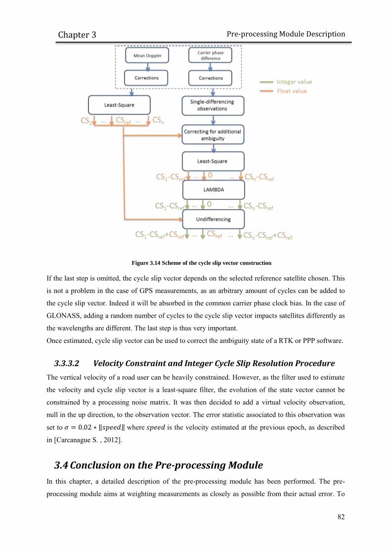
82
Pre-processing Module Description
Chapter 3
Figure 3.14 Scheme of the cycle slip vector construction
If the last step is omitted, the cycle slip vector depends on the selected reference satellite chosen. This
is not a problem in the case of GPS measurements, as an arbitrary amount of cycles can be added to
the cycle slip vector. Indeed it will be absorbed in the common carrier phase clock bias. In the case of
GLONASS, adding a random number of cycles to the cycle slip vector impacts satellites differently as
the wavelengths are different. The last step is thus very important.
Once estimated, cycle slip vector can be used to correct the ambiguity state of a RTK or PPP software.
3.3.3.2 Velocity Constraint and Integer Cycle Slip Resolution Procedure
The vertical velocity of a road user can be heavily constrained. However, as the filter used to estimate
the velocity and cycle slip vector is a least-square filter, the evolution of the state vector cannot be
constrained by a processing noise matrix. It was then decided to add a virtual velocity observation,
null in the up direction, to the observation vector. The error statistic associated to this observation was
set to ‖ ‖ where is the velocity estimated at the previous epoch, as described
in [Carcanague S. , 2012].
3.4 Conclusion on the Pre-processing Module
In this chapter, a detailed description of the pre-processing module has been performed. The pre-
processing module aims at weighting measurements as closely as possible from their actual error. To

83
Pre-processing Module Description
Chapter 3
do so, code and Doppler measurement errors due to multipath have been analyzed and a weighting
scheme has been derived. Moreover, code and Doppler measurements outliers are detected and
excluded using the so-called Danish method. Additionally GPS/GLONASS cycle slips are estimated
as integers, using an innovative cycle slip resolution technique. Finally, GLONASS code
measurements are corrected from non-linear inter-channel biases and appropriately down-weighted
relative to GPS pseudoranges. A general scheme of the pre-processing module can be found on Figure
3.15.
Figure 3.15 General scheme of the pre-processing module
In the next chapter, the positioning filter implementation will be described.

84
GPS/GLONASS Precise Positioning Filter Design
Chapter 4
Chapter 4. GPS/GLONASS Precise Positioning Filter Design
The preprocessing module described previously aims at correcting, selecting and classifying
measurements available in function of their quality. However, designing a RTK filter for low-cost
GPS/GLONASS positioning in difficult environment can be challenging even if the measurement
selection and classification performs well. Indeed:
Low-cost receivers will not be time-synchronized to the reference receiver. The difference
between the time of measurement of the reference station and the time of measurement of the
rover can be significant.
GLONASS carrier phase measurements are biased by inter-channel delays which are receiver-
specific.
As the number of tracked signals can be reduced (coming from less than 4 satellites), the state
variables have to be updated in low-visibility conditions.
GSM data link outages can prevent from frequent reference station data update.
These issues have driven a number of choices in the design of the RTK software that will be described
in the different sub-sections of this chapter.
4.1 Standard Kalman Filtering Theory
Kalman filter is a recursive algorithm that allows the optimal parametric estimation of a state vector
characterizing a system [Kubrak, 2007]. Contrary to Least-Square algorithm which provides an
estimate that relies only on the measurements of the current epoch, Kalman filter combines the
observation from the current epoch with the state prediction obtained from previous epochs to update
the state variables, as well as the associated error covariance.
Kalman filter is commonly used in GNSS algorithms to fuse receiver measurements with additional
sensors (IMU, LiDAR…) or to estimate a trajectory knowing information on the vehicle dynamic.
4.1.1 General State Model
The general state model for a continuous linear system can be expressed as [Kubrak, 2007]:
{ ( ) ( ) ( ) ( )
( ) ( ) ( ) ( )
Where:

85
GPS/GLONASS Precise Positioning Filter Design
Chapter 4
( ) is the state vector at time
( ) is the state transition matrix
( ) is the state noise vector characterized by its covariance matrix ( )
( ) is the observation function
( ) is the observation vector
( ) is the measurement noise
If the state is a continuous process observed at discrete epochs with periods , the system can be
discretized, using Taylor series. The system then becomes [Kubrak, 2007]:
{
Where:
( ) the state vector at epoch
( ( ) ) ( ) ( ( ) )
(
) is the state transition matrix.
is the state noise vector characterized by its covariance matrix
with ( ) ( ( ) ( ) ( ) ( ) )
(
)
( )
( )
is the measurement noise vector characterized by its covariance matrix ( )
4.1.2 Kalman Filter Equations
The Kalman filter allows to recursively estimate state variables of a system as well as their associated
covariance matrix. It consists in 5 equations:
|
(
)
| [ ]
Where:
is a posteriori state estimate, with associated covariance matrix

86
GPS/GLONASS Precise Positioning Filter Design
Chapter 4
The Kalman filter is limited to the case that ( ) and ( ) are linear. If they are nonlinear as it is
usually the case in GNSS systems, an Extended Kalman filter can be used instead.
4.1.3 Linearization of the Model: the Extended Kalman Filter
The Extended Kalman filter is a generalization of the Kalman filter when the state transition function
and/or the observation function are non-linear. Similarly to the Kalman filter, the Extended Kalman
filter is composed of 5 equations which are iterated:
| ( )
(
)
| [ ( )]
Where:
( ) and
( )
In the following, the structure of the Extended Kalman filter used in the RTK algorithm will be
described. This filter is used to estimate position, velocity and acceleration together with
GPS/GLONASS ambiguities, GLONASS code inter-channel biases and differential receiver clock
bias.
4.2 RTK Kalman Filter Description
4.2.1 Observation Vector
4.2.1.1 Input Measurements
As pointed out in 2.2.2.1, differencing measurements from 2 close receivers removes spatially
correlated errors. Once this first difference is performed, the observation vector can be expressed
through different formulations. For instance either single differences or double differences can be
formed with code and carrier phase, and for GPS and GLONASS measurements. Moreover, if double
differences are used, a unique reference satellite or a separate one for each constellation can be chosen.
[Wang, et al., 2001] has isolated 18 possible ways to express the observation vector from the same
initial GPS/GLONASS code and carrier phase measurements. However, all implementations are not

87
GPS/GLONASS Precise Positioning Filter Design
Chapter 4
equivalent in terms of, for instance, minimum number of observations to estimate a position, easiness
of implementation and possibility to estimate ambiguities as integers.
The following implementation was chosen in the filter:
GPS code measurements are single-differenced.
GPS carrier phase measurements are double-differenced
GLONASS code measurements are single-differenced
GLONASS carrier phase measurements are single-differenced.
Many advantages drove the choice for using only single-differenced code measurements for both
constellations [Kozlov, et al., 1997]. First, it removes any problem related to the choice or the change
of the reference satellite. Moreover the pseudorange outlier detection module uses only single-
differenced code measurements, as explained in 3.2. Then code inter-channel biases estimated in the
RTK filter can be directly used in the outlier detection module to correct GLONASS code
measurements. Finally, it avoids any further correlation of code measurements due to double-
differencing.
As pointed out in 2.2.2.1, GPS carrier phase measurements have to be double-differenced in order to
estimate carrier phase ambiguities as integers. On the other hand, GLONASS carrier phase
measurements are kept in single-difference mode as the single difference ambiguity is required to
estimate GLONASS double-differenced ambiguities as integers, as explained in 2.2.2.2.
In the Kalman filter, GPS single-differenced code and double-differenced carrier phase are classically
modeled as:
|
(4.1)
Where:
and are the single and the double-differenced geometric range
is the receiver clock offset difference and c is the speed of light
is the carrier phase ambiguity
is the carrier phase wavelength
However, GLONASS single-differenced code and carrier phase measurement model in the Kalman
filter is simplified to:
|
(4.2)
Where and are the pseudoranges receiver hardware bias and code inter-channel biases slope
respectively, is the GLONASS frequency number. In equation (4.2), code inter-channel biases are
modeled as a linear function of the GLONASS frequency number, as observed for high-end receiver in
chapter 2. This model is true with the tested NVS receiver only if it is calibrated, as explained in

88
GPS/GLONASS Precise Positioning Filter Design
Chapter 4
3.1.1.4. However, single-differenced carrier phase are modeled as having the same receiver hardware
bias as single-differenced code measurements. It is not true in practice as explained in 2.2.2.2 but this
simplification has no impact as long as GLONASS ambiguities are estimated as floats, as the
unmodeled carrier phase inter-channel bias will be lumped into the float ambiguity estimate.
The receiver clock offset difference is common to both GPS and GLONASS model, as it is a time
difference independent of the time system.
Similarly to the multipath detection and exclusion module, only rover Doppler measurements were
used, as some reference stations don’t provide raw Doppler data. Code, Doppler and carrier phase
measurements are weighted using the weighting schemes presented in Chapter 3.
Finally, the observation vector includes a virtual velocity observation, null in the up direction.
Similarly to 3.3.3.2, the virtual velocity is weighted as a function of the estimated velocity, following
equation (4.3):
‖ ‖ (4.3)
where is the user velocity estimated at the previous epoch.
4.2.1.2 Linearization Process and Measurement Corrections
A non-linear relationship exists between single-differenced or double-differenced range and the rover
position. Therefore the system has to be linearized in order to estimate the rover position from code
and carrier phase measurements, using an extended Kalman filter.
Following [Realini, 2009], between-receiver range difference for satellite can be linearized around
the rover predicted position:
(
) ([
]
[ ]
) (4.4)
Where:
is the between-station range difference as measured by single-
differenced code or single-differenced carrier phase
is the line-of-sight vector from the rover approximate position, obtained from the
Kalman filter prediction, to the estimated satellite position
is the range from the rover approximate position to the estimated satellite position
[ ]
is the predicted rover position obtained from the Kalman filter

89
GPS/GLONASS Precise Positioning Filter Design
Chapter 4
[ ]
is the estimated rover position
Therefore, GPS and GLONASS code and carrier phase observations are corrected to obtain a linear
relationship with rover position. Additionally, differential tropospheric delay correction as modeled by
UNB3m [Leandro, et al., 2006], differential ionospheric delay correction as modeled by the Klobuchar
model in broadcast ephemeris and differential satellite clock offset correction obtained from ephemeris
are applied. For instance GPS single-differenced code measurements are corrected as such:
(
)
[ ]
(4.5)
Where:
is the differential ionospheric delay correction obtained with Klobuchar model.
is the differential tropospheric delay correction obtained with UNB3m model.
is the differential satellite clock offset correction. Satellite clock offset correction can be
slightly different at both end of the baseline, as measurement times are different.
It can be noticed that the linearized observation depends only on the satellite geometry at the rover
linearized position and at rover measurement time. Therefore, any short delay in measurement time
between the reference receiver and the rover has no impact on the estimation provided that
atmospheric, satellite clock and orbit differential error remains negligible. In particular, the
experienced millisecond-level delay between the NVS receiver measurement time and the reference
station measurement time due to the fact that the NVS receiver clock is not steered to GPS time has no
impact on the positioning software provided at the second level, as denoted in [Odijk, et al., 2007].
Therefore, no time extrapolation was applied to reference or rover data.
4.2.1.3 Doppler Measurements Correction
The Doppler frequency shift as measured by the receiver is an observation of the relative motion of the
satellite relative to the rover antenna, including relative clock drift [Kaplan, et al., 2006]. To estimate
the rover velocity from Doppler measurements, the Doppler shift due to the satellite velocity first has
to be removed. Doppler measurements are corrected as such [Angrisano, 2010]:
[
]
[
]
( )
(4.6)
Where:

90
GPS/GLONASS Precise Positioning Filter Design
Chapter 4
[
]
is the satellite velocity vector, as computed from broadcast ephemeris
[
]
is the rover velocity vector
The satellite clock offset rate, the ionospheric delay rate and the tropospheric delay rate are considered
negligible and are not corrected in the software.
As seen on equation (4.12), no linearization has to be performed for velocity estimation using Doppler
measurements, as the corrected Doppler is directly the projection of the receiver velocity on the
receiver to satellite line-of-sight vector.
4.2.2 State Vector
In view of the targeted application, the position, velocity and potentially acceleration are the only
parameters of importance for the user. However, considering the structure of the observation vector,
additional parameters have to be estimated:
First, as GPS and GLONASS code pseudoranges are only single-differenced, a between-
station clock bias difference has to be estimated, as well as its rate.
Additionally, GLONASS inter-channel biases have to be estimated. To do so, they are
modeled as a linear function of the frequency, i.e. a slope and an offset are estimated. Indeed
NVS-08C code inter-channel biases are calibrated only relative to a specific brand of high-end
receiver, as explained in 3.1.1.4.
Finally, as the rover Doppler measurements are related to the rover clock rate and not to the
differential clock rate, an instantaneous rover clock rate state is added to the state vector. A
scheme of the Kalman filter structure can be found on Figure 4.1.
Figure 4.1 Scheme of the implemented RTK Kalman filter
4.2.3 State Transition Model and Process Noise

91
GPS/GLONASS Precise Positioning Filter Design
Chapter 4
In a Kalman filter, the variation of the different parameters from an epoch to the other has to be
modeled as accurately as possible.
As explained in the previous section, position, velocity and acceleration of the vehicle are estimated
explicitly in the Kalman filter, as in [Realini, 2009]. The Kalman filter transition matrix is described
on Figure 4.2, following [Realini, 2009].Only the first order is considered. is the time difference
between 2 adjacent epochs.
Figure 4.2 Transition matrix of the RTK Kalman filter
The process noise matrix is added to the acceleration covariance after each prediction of the filter. As
seen in 2.4.5, the vertical motion of a vehicle can be constrained in the case of car navigation.
Therefore, the process noise added to the acceleration covariance matrix is associated to a lower
variance in the up direction. To do so, the process noise added to the vehicle acceleration covariance is
described in the “East-North-Up” local frame and transformed in ECEF frame following noise
propagation laws:
[
] (4.7)
Where:

92
GPS/GLONASS Precise Positioning Filter Design
Chapter 4
,
, are the variance associated to the process noise added to acceleration in the “East-
North-Up” local frame. These variances depend on the vehicle dynamic.
[
( ) ( )
( ) ( ) ( ) ( ) ( )
( ) ( ) ( ) ( ) ( )] and and are the
latitude and the longitude of the rover in radians [Sanz Subirana, et al., 2011].
The slope and the offset of GLONASS code inter-channel biases are estimated as constant values,
provided the receiver is not powered off during data collection. More details on GLONASS code inter-
channel bias offset stability are given in section 4.2.7.1.
Similarly, ambiguities are estimated as constant as long as cycle slips are monitored and resolved.
Therefore, no process noise is added to their covariance matrix.
Regarding clock bias evolution, the process noise added to the differential clock rate variance and the
Doppler rate variance was set to a few hundred meters. The structure of the process noise matrix is
summarized on Figure 4.3.
Figure 4.3 Structure of the RTK Kalman filter process noise matrix
The variance values chosen in the software will be presented in Chapter 5.
4.2.4 Design Matrix
Considering the observation vector and the state vector structures presented in 4.2.1 and 4.2.2, the
RTK Kalman filter is built as such:

93
GPS/GLONASS Precise Positioning Filter Design
Chapter 4
As presented in 4.2.1.2, the linearized observed range difference is the projection of the
estimated position on the line-of-sight vector, computed at the rover predicted position. In the
case of double-differenced observations, the line-of-sight vector is simply differenced
between satellites.
Corrected Doppler measurements are the projection of the estimated velocity on the opposite
direction of the line-of-sight vector.
GLONASS pseudoranges inter-channel biases are also estimated, as a linear function of the
GLONASS frequency number associated to the satellite .
Ambiguities are estimated in cycles and therefore linked to carrier phase measurements via
their respective wavelengths.
The null vertical velocity observation is linked to the estimated speed by using the normalized
rover predicted coordinates, as this vector points in the up direction. The normalized rover
coordinates vector is obtained following equation (4.14):
[
]
[ ]
‖[ ]
‖
(4.8)
RTK filter design matrix is summarized on Figure 4.4.

94
GPS/GLONASS Precise Positioning Filter Design
Chapter 4
Figure 4.4 Structure of the RTK filter design matrix
In the case GLONASS ambiguity are estimated as integers, a slightly different design matrix is used,
as explained in 4.2.7.2.
4.2.5 Geometry Configuration Changes and Cycle Slips Correction
As satellite elevation and azimuth change with time, the constellation geometry evolves and satellites
appear and disappear. Moreover, as satellite signal blockage can be very frequent in urban
environment, the RTK software has to handle smoothly any satellite configuration change.
4.2.5.1 Availability of a new satellite carrier phase measurement
Contrary to code measurements which can appear or disappear without changing the size of the state
vector, the tracking of a new carrier phase measurement involves the estimation of a new ambiguity

95
GPS/GLONASS Precise Positioning Filter Design
Chapter 4
state and therefore the initialization of this state. Ambiguities initialization is performed using the
predicted state value. In the case of a GPS carrier phase observation, the double-differenced ambiguity
is initialized using the predicted double-differenced range:
(4.9)
Where:
is the double-differenced range obtained using the Kalman filter predicted rover
position.
In the case of GLONASS satellites, single-differenced carrier phase ambiguities are initialized as
such:
(4.10)
Where:
is the single differenced range obtained using Kalman filter predicted rover position.
is the predicted between-station clock bias obtained from Kalman filter.
A diagonal matrix with high variance values is associated to initialized ambiguities.
4.2.5.2 Reference satellite change
In the Kalman filter, GPS carrier phase measurements are double-differenced, whereas, GLONASS
carrier phase measurements are single-differenced. Therefore, a reference satellite is needed only for
GPS carrier phase measurements. It is chosen as the visible satellite with the highest C/N0 value. In the
case of a reference satellite change from satellite to , the state vector and the covariance matrix are
rotated, following equation:
|
(4.11)
Where:
and
are the state vector with reference satellite and respectively
and
are the covariance matrix with reference satellite and respectively
is the rotation matrix described on Figure 4.5.

96
GPS/GLONASS Precise Positioning Filter Design
Chapter 4
Figure 4.5 Rotation matrix related to reference satellite j
4.2.5.1 Cycle Slip Correction
A cycle slip resolution module has been proposed in 3.3. Two cases can occur:
A cycle slip is detected but the estimated integer cycle slip vector does not pass the validation
test. In that case, the ambiguity state is reinitialized as in 4.2.5.1, similarly as if new carrier
phase measurements were available.
A cycle slip is detected and the estimated integer cycle slip passes the validation test. In that
case, the cycle slip values related to GPS satellites are first differenced with the cycle slip
value of the current GPS reference satellite. Then, the cycle slip vector is subtracted from the
ambiguity state, while the state covariance matrix remains untouched.
4.2.6 Carrier Phase Integer Ambiguity Resolution
As explained earlier, the LAMBDA method is used to estimate the integer ambiguities from the float
ambiguity state vector and covariance matrix. However, a number of conditions are required to
validate the integer vector and consider it as the true value. Indeed, the validation of the integer vector
is a critical step, as a wrong integer fix can propagate through multiple epochs in the Kalman filter,
potentially strongly biasing the position estimate.

97
GPS/GLONASS Precise Positioning Filter Design
Chapter 4
First, a minimum of 5 float ambiguities is required to start the integer ambiguity resolution. Indeed,
setting the minimum number of ambiguities to a high value was shown to improve the reliability of the
ratio-test [Shirai, et al., 2011]. Secondly, the ratio-test is performed. It is defined as [Teunissen, et al.,
2004]:
‖ ‖
‖ ‖
Where:
the float ambiguity vector
its covariance matrix
and are the first and second best integer solution.
Different values for will be tested in Chapter 6. As [Shirai, et al., 2011] showed that stricter
validation parameters were required in urban environments, validation parameters depending on the
type of environment will be tested.
If one of this validation test fails, the state vector and its covariance remains untouched and the next
epoch is processed. On the other hand, if the integer ambiguity vector is successfully validated, the
state vector and its related covariance matrix are adjusted using the new integer ambiguity vector. First
the float ambiguities are replaced by the fixed ambiguities and their associated covariance matrix is set
to a very low value, such as a variance of 0.0001 cycle in the software. Then, other parameters
composing the state vector are adjusted using the integer ambiguities instead of the float ambiguities.
Considering that the state vector is composed of and (the state vector of the GPS ambiguities
and the state vector of the other parameter respectively), the state vector and its covariance matrix
can be expressed as:
[
]
[
]
(4.12)
Then, the state vector of the other parameters is adjusted as such [Teunissen P. , 1995]:
( ) (4.13)
The covariance matrix of the other parameters is similarly adjusted:
(4.14)
Integer ambiguity resolution, validation and adjustment of other parameters are performed at each
epoch using the entire ambiguity vector, independently from the fact that some ambiguities were
potentially fixed at previous epoch or not.

98
GPS/GLONASS Precise Positioning Filter Design
Chapter 4
4.2.7 GLONASS Carrier Phase Integer Ambiguity Resolution
In the case of GPS measurements, double-differenced ambiguities and their associated covariance
matrix estimated in the Kalman filter are directly used as input of the LAMBDA algorithm. In
GLONASS case, integer ambiguities cannot be estimated directly from Kalman filter float single-
differenced ambiguities. They need to be transformed and corrected.
Indeed, the model used for GPS measurements in the Kalman filter is:
|
(4.15)
while the model used for GLONASS measurements is:
|
(4.16)
Although commonly used, these 2 measurement models are incomplete. Indeed, following chapter 2
the code and carrier phase Kalman filter observation model for GPS and GLONASS constellations:
||
(4.17)
Where
and are GPS and GLONASS code receiver hardware delays.
and are carrier phase receiver hardware bias and inter-channel bias respectively. It
can be denoted that , , are independent of the frequency, contrary to
.
All measurements share the same oscillator and therefore are affected by the same receiver clock
offset
Thus, the GLONASS single-differenced ambiguity estimate obtained using the incomplete model in
the Kalman filter can be expressed as:
(4.18)
Where
(4.19)
is the difference between GPS and GLONASS differential code receiver hardware biases.
To estimate GLONASS carrier phase ambiguities as integers, 3 steps are proposed:
Differencing between satellites the single-differenced float ambiguities (in meters):

99
GPS/GLONASS Precise Positioning Filter Design
Chapter 4
( )
(4.20)
Removing the single-differenced ambiguity using float estimate
( )
( )
( )
(4.21)
As explained in 2.2.2.2, the maximum wavelength of the additional ambiguity is (
) . As this value is extremely small, a rough estimate of , such as the
float estimate provided by the RTK Kalman filter can be used and the quantity ( )
can be removed. However, this process further bias double differenced ambiguities with an
additional offset function of both carrier phase and code inter-channel biases.
Removing the bias ( )
( ) from double differenced
ambiguities after determining its value using an initial calibration phase. This offset has to be
known at mm-level, in order not to bias GLONASS carrier phase measurements
systematically. Therefore, it is a more delicate phase as the entire ambiguity resolution process
can be jeopardized if the bias correction is not precise enough. Table values exist for most
high-end receiver brands, as in [Wanninger L. , 2011]. However, no such table exist for the
NVS-08C. Moreover, it was shown in 2.5.2.3 that these biases could be different between 2
NVS-08C with similar firmware. Therefore, the navigation software has to be able to correct
receivers from carrier phase inter-channel biases individually.
This calibration is described in the next section.
4.2.7.1 GLONASS Carrier Phase Inter-channel Biases Calibration
The most precise way to calibrate carrier phase inter-channel biases is to perform a zero-baseline
between the rover and the reference station, as in [Al-Shaery, et al., 2012]. However, it is not a very
practical technique, as it requires having physically access to both the rover and the reference station
receiver. Therefore, an algorithm for GLONASS inter-channel calibration is proposed on Figure 4.6. It
has the advantage to be very easily implemented as a “add-on” of the previously described RTK filter,
as it only requires GLONASS estimated single-differenced ambiguities.

100
GPS/GLONASS Precise Positioning Filter Design
Chapter 4
Figure 4.6 Scheme of the carrier phase inter-channel bias calibration algorithm
In order to isolate GLONASS carrier phase inter-channel biases, the algorithm performs as follow:
Double-differenced GPS ambiguities are first estimated and fixed using the LAMBDA
method, while single-differenced GLONASS ambiguities are estimated as floats.
In the case double-differenced GPS ambiguities are validated, other parameters, including
GLONASS single-differenced ambiguities are adjusted, as explained in 4.2.6. Then
GLONASS single-differenced float ambiguities with an accuracy of a few hundreds of a cycle
relatively to each other are obtained.
Each GLONASS carrier phase ambiguity is then multiplied by its associated wavelength and
double-differenced. Single-differenced ambiguity is removed and the result is passed in cycle
by dividing by the reference satellite wavelength. Equation (4.21) becomes:
( )
( )
( )
(4.22)
[Sleewaegen, et al., 2012] shows that is at the tenth-of-millimeter level independently of
the frequency and that most part of the bias is due to the difference between carrier phase

101
GPS/GLONASS Precise Positioning Filter Design
Chapter 4
hardware bias and code hardware bias ( ) . As ( )
is a function of the
difference between GLONASS frequency numbers ( ) , the inter-channel bias is
expected to be a function of the GLONASS frequency number difference.
Therefore, equation (4.22) is rewritten:
( )
( ) (4.23)
Finally, closest integer is removed from equation (4.23). As is an integer, this step
isolates ( ) modulo a cycle.
If the 2 receivers were high-end receivers of the same brand, the difference between equation (4.23)
and closest integer should be very close to zero as on Figure 4.8. However, in the case of 2 receivers of
different brands, biases remain, as seen on Figure 4.7 between a Trimble and a Leica receiver.
Figure 4.7 Difference between adjusted GLONASS double-
differenced ambiguities corrected from the single-differenced
ambiguity and the closest integer on January 5th, 2012, between TLSE
reference station (Trimble receiver) and TLIA rover receiver (Leica
receiver). Stations are separated by 90 meters.
Figure 4.8 Difference between adjusted GLONASS double-
differenced ambiguities corrected from the single-differenced
ambiguity and the closest integer on January 5th, 2012, between
TLMF reference station (Leica receiver) and TLIA rover receiver
(Leica receiver). Stations are separated by 8 kms.
Then is estimated by mapping each inter-channel biases to its associated GLONASS
frequency number.
An important remark is that biases are linear with frequency in cycle. However, as biases on
each channel are obtained after rounding off equation (4.23), the result may not be linear if the
maximum bias amplitude exceeds one cycle. An example can be found on Figure 4.9 with the
Trimble/Leica baseline. In that case, the bias in meters is approximately -0.03 meters times the
frequency number [Wanninger L. , 2011]. Dividing this bias by the reference satellite
wavelength and removing the closest integer gives a nonlinear function over GLONASS
frequency band, as seen on Figure 4.9. Therefore it is recommended to first roughly estimate
0 500 1000 1500 2000 2500 3000 3500-0.5
-0.4
-0.3
-0.2
-0.1
0
0.1
0.2
0.3
0.4
0.5Isolated GLONASS interchannel biases
epochs (1Hz)
Cycle
0 500 1000 1500 2000 2500 3000 3500-0.5
-0.4
-0.3
-0.2
-0.1
0
0.1
0.2
0.3
0.4
0.5Isolated GLONASS interchannel biases
epochs (1Hz)
Cycle

102
GPS/GLONASS Precise Positioning Filter Design
Chapter 4
the slope between 2 adjacent frequencies apply the first correction and refine the bias
estimation in a second step. Additionally it can be seen on Figure 4.9 that the carrier phase
inter-channel biases found using the presented calibration method matches well the value
proposed by [Wanninger L. , 2011].
Figure 4.9 Estimated carrier phase inter-channel biases as a
function of GLONASS frequency number for a baseline between
TLSE reference station (Trimble receiver) and TLIA rover receiver
(Leica receiver). The linear model for a Leica-Trimble baseline from
[Wanninger L. , 2011] is plotted in black.
Figure 4.10 Difference between adjusted GLONASS double-
differenced ambiguities corrected from the single-differenced
ambiguity and the closest integer on January 5th, 2012, between
TLSE reference station (Trimble receiver) and TLIA rover
receiver (Leica receiver) after applying the correction proposed
by [Wanninger L. , 2011].
Finally, biases are multiplied by the reference satellite wavelength to obtain a calibration value
in meters that is independent of the reference satellite chosen. The difference between adjusted
GLONASS double-differenced ambiguities corrected from the single-differenced ambiguity
and the closest integer for the Trimble/Leica baseline is plotted on Figure 4.10, after applying
the estimated biases. It can be seen that the remaining residuals have an amplitude below 0.1
cycle.
The proposed calibration algorithm can be performed in 2 ways:
Carrier phase inter-channel bias slope can be estimated continuously.
It can be estimated during an initial calibration phase and used as a-priori value during the
operational phase of the rover.
The first way has the advantage of not requiring any input from the user. The filter performs the
calibration itself. However, in the case of a wrong fix of GPS ambiguities and therefore wrong
calibration value estimates, the ambiguity resolution may be jeopardized. Then, estimating GPS and
GLONASS integer ambiguities altogether would give a worst result than estimating GPS integer
ambiguities alone.
The second solution allows controlling the quality of the carrier phase inter-channel bias slope
estimate, by using only a clear-sky environment data set. It was the preferred choice as the reliability
of GPS ambiguity fixing with a low-cost receiver in difficult environment is uncertain. However, to
-6 -4 -2 0 2 4 6-0.5
-0.4
-0.3
-0.2
-0.1
0
0.1
0.2
0.3
0.4
0.5
GLONASS frequency number
Cycle
Isolated GLONASS interchannel biases as a function of GLONASS frequency number
Estimated carrier phase biases
Linear model [Wanninger, 2011]
0 500 1000 1500 2000 2500 3000 3500-0.5
-0.4
-0.3
-0.2
-0.1
0
0.1
0.2
0.3
0.4
0.5Isolated GLONASS interchannel biases
epochs (1Hz)
Cycle

103
GPS/GLONASS Precise Positioning Filter Design
Chapter 4
avoid performing the calibration at each receiver start, the carrier phase inter-channel bias slope has to
be stable in time.
4.2.7.2 Time Variation of GLONASS Carrier Phase Inter-channel Biases
with a Low-cost Receiver
As explained in the previous section, the GLONASS carrier phase bias on each channel depends on
the difference between differential code measurement hardware bias and differential carrier phase
hardware bias .
Hence any variation of or can translate into a variation of the GLONASS
carrier phase bias on each channel after correcting for additional ambiguity. As the correction method
for carrier phase inter-channel biases is based on a-priori values obtained from a calibration algorithm
proposed in the previous section, the variation of the bias has to be very small so that the user does not
need to perform the calibration frequently.
In order to determine if is stable on a few days scale, 2 static data collections are performed,
using the NVS-08C receiver connected to a patch antenna. The patch antenna was placed on top of a
building, in a clear sky environment. The first data collection is performed on June 22nd 2012, while
the second is performed on July, 3rd 2012. A baseline is formed with TLSE (Trimble receiver). The
NVS-08C receiver was completely powered off between the 2 data collections.
The offset between GPS code differential receiver clock and GLONASS code differential receiver
clock was estimated and was found to vary by a few meters between the
different data collections, as seen on Table 4.1. Table 4.1 Values of estimates, for 2 separated data collections, using a NVS-08C connected to a
patch antenna. TLSE (Trimble receiver) was used as reference station.
June 22nd, 2012 July 3rd, 2012
Estimated
116 meters 121.5 meters
Variations of a few meters of were empirically noticed as occurring when the
receiver was powered off.
In order to determine the impact of such a variation on carrier phase inter-channel biases using same
multipath and geometry conditions, GLONASS carrier phase residuals, i.e. the difference between
double-differenced GLONASS carrier phase corrected from single-differenced ambiguity and the
nearest integer is plotted Figure 4.11 and Figure 4.12 for June 22nd, 2012. In both plots, an a-priori
calibration value of 4.41cm for 2 adjacent GLONASS frequencies was removed. In Figure 4.11,
GLONASS pseudoranges remained untouched. In Figure 4.12, 5 meters were added to each
GLONASS pseudoranges. This 5 meters addition on every GLONASS pseudorange doesn’t change
the float solution accuracy, as it is merged in the differential clock estimate. However, it shifts the

104
GPS/GLONASS Precise Positioning Filter Design
Chapter 4
value of by 5 meters. Therefore, the value of the single-differenced ambiguity
used to correct the double-differenced carrier phase measurements is also shifted by approximately 26
cycles. As seen on Figure 4.12, such a change makes the GLONASS carrier phase inter-channel biases
vary significantly.
Figure 4.11 Double-differenced carrier phase residuals with
the closest integer, after applying an a-priori correction of 4.41 cm
for 2 adjacent frequencies, with a data set collected on June 22nd,
2012.
Figure 4.12 Double-differenced carrier phase residuals
with the closest integer, after applying an a-priori correction
of 4.41 cm for 2 adjacent frequencies, with a data set collected
on June 22nd, 2012. In this case, 5 meters have been added to
all GLONASS pseudoranges.
Therefore, variations in time of make long-term accurate calibration of GLONASS
carrier phase of the NVS receiver impossible using classic Kalman filter observation model.
4.2.7.3 Proposed Strategy to Limit the Time Variation of GLONASS
Carrier Phase Inter-channel Biases
It is not possible to know a-priori if the variation noticed in Table 4.1 comes from GPS receiver
hardware bias variation, GLONASS receiver hardware bias variation or both.
In order to determine if the GLONASS carrier phase inter-channel variation mostly comes from GPS
code measurements or GLONASS code measurements, a test is performed, using 2 data sets separated
by 4 months interval. The first data set is the one collected on June 22nd and described in the previous
section. The second was collected on October 3rd, 2012. Once again, a baseline was formed between
the same NVS-08C receiver equipped with patch antenna and TLSE Trimble receiver. On October 3rd
data collection, was estimated around 109 meters.
Each data set is processed using 2 different simplified measurement model in the Kalman filter:
Considering GLONASS carrier phase measurements and GLONASS pseudoranges share a
common differential receiver clock offset , composed of reference oscillator and a
common receiver hardware bias:
0 50 100 150 200 250 300 350 400-0.5
-0.4
-0.3
-0.2
-0.1
0
0.1
0.2
0.3
0.4
0.5Isolated GLONASS interchannel biases
epochs (1Hz)
Cycle
0 50 100 150 200 250 300 350 400-0.5
-0.4
-0.3
-0.2
-0.1
0
0.1
0.2
0.3
0.4
0.5Isolated GLONASS interchannel biases
epochs (1Hz)
Cycle

105
GPS/GLONASS Precise Positioning Filter Design
Chapter 4
||
(4.24)
It is the model used in the previous sections.
Considering GLONASS carrier phase measurements and GPS pseudoranges share a common
differential receiver clock offset and receiver hardware bias:
||
(4.25)
In the first case, the design matrix of the Kalman filter can be found on Figure 4.13. In the second
case, it can be found on Figure 4.14. The difference between the 2 design matrices is underlined in red.

106
GPS/GLONASS Precise Positioning Filter Design
Chapter 4
Figure 4.13 Structure of the RTK filter design matrix when GLONASS measurements are leveled by GLONASS
pseudoranges.

107
GPS/GLONASS Precise Positioning Filter Design
Chapter 4
Figure 4.14 Structure of the RTK filter design matrix when GLONASS measurements are leveled by GPS
pseudoranges.
For both data sets and both types of processing, biases are estimated using the calibration method
described in 4.2.7.1. An a-priori calibration value of 4.41cm for 2 adjacent frequencies is applied for
the first type of processing while an a-priori calibration value of 4.7mm for 2 adjacent frequencies is
applied in the second type, for both data sets. Results can be found on Figure 4.15 and Figure 4.16 for
the first data set, and Figure 4.17 and Figure 4.18 for the second data set.
It can be seen that when GLONASS carrier phase measurements are assumed to share the same
receiver clock than GPS pseudorange, the GLONASS carrier phase inter-channel bias has almost not
varied although both data collections are separated by a few months and has
varied. However, variations of GLONASS carrier phase inter-channel bias can be denoted if
GLONASS carrier phase are assumed to share the same receiver clock than GLONASS pseudorange.
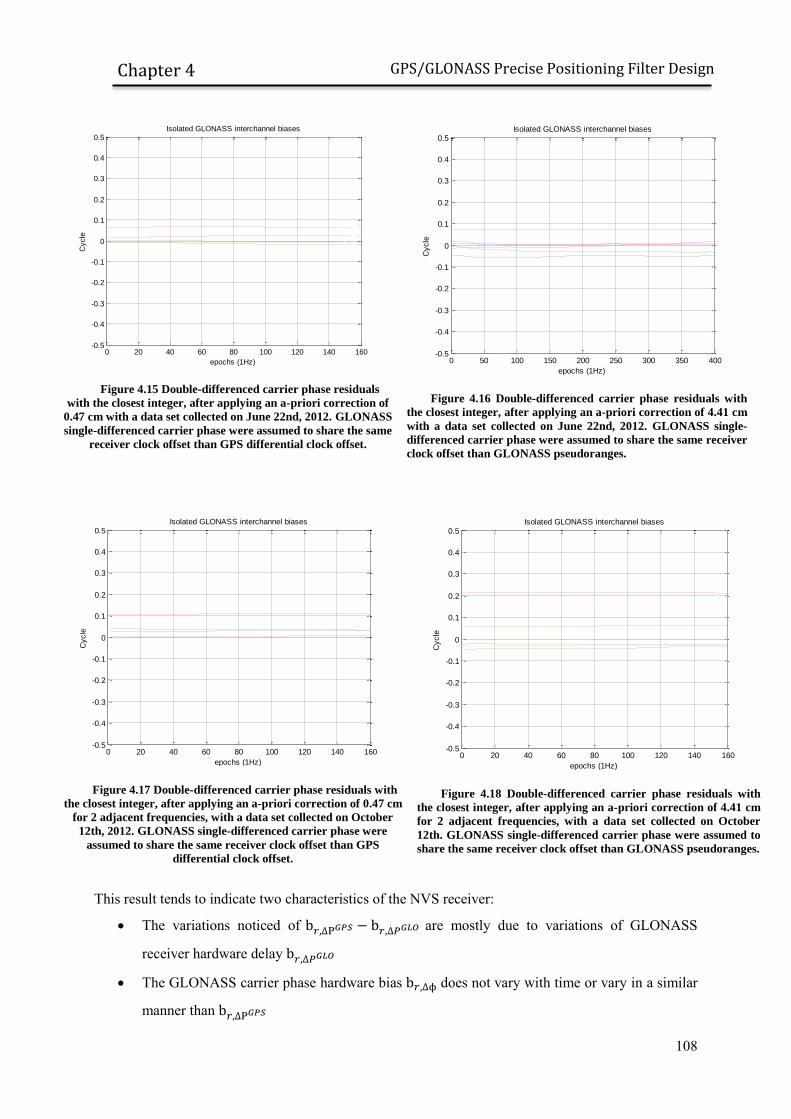
108
GPS/GLONASS Precise Positioning Filter Design
Chapter 4
Figure 4.15 Double-differenced carrier phase residuals
with the closest integer, after applying an a-priori correction of
0.47 cm with a data set collected on June 22nd, 2012. GLONASS
single-differenced carrier phase were assumed to share the same
receiver clock offset than GPS differential clock offset.
Figure 4.16 Double-differenced carrier phase residuals with
the closest integer, after applying an a-priori correction of 4.41 cm
with a data set collected on June 22nd, 2012. GLONASS single-
differenced carrier phase were assumed to share the same receiver
clock offset than GLONASS pseudoranges.
Figure 4.17 Double-differenced carrier phase residuals with
the closest integer, after applying an a-priori correction of 0.47 cm
for 2 adjacent frequencies, with a data set collected on October
12th, 2012. GLONASS single-differenced carrier phase were
assumed to share the same receiver clock offset than GPS
differential clock offset.
Figure 4.18 Double-differenced carrier phase residuals with
the closest integer, after applying an a-priori correction of 4.41 cm
for 2 adjacent frequencies, with a data set collected on October
12th. GLONASS single-differenced carrier phase were assumed to
share the same receiver clock offset than GLONASS pseudoranges.
This result tends to indicate two characteristics of the NVS receiver:
The variations noticed of are mostly due to variations of GLONASS
receiver hardware delay
The GLONASS carrier phase hardware bias does not vary with time or vary in a similar
manner than
0 20 40 60 80 100 120 140 160-0.5
-0.4
-0.3
-0.2
-0.1
0
0.1
0.2
0.3
0.4
0.5Isolated GLONASS interchannel biases
epochs (1Hz)
Cycle
0 50 100 150 200 250 300 350 400-0.5
-0.4
-0.3
-0.2
-0.1
0
0.1
0.2
0.3
0.4
0.5Isolated GLONASS interchannel biases
epochs (1Hz)
Cycle
0 20 40 60 80 100 120 140 160-0.5
-0.4
-0.3
-0.2
-0.1
0
0.1
0.2
0.3
0.4
0.5Isolated GLONASS interchannel biases
epochs (1Hz)
Cycle
0 20 40 60 80 100 120 140 160-0.5
-0.4
-0.3
-0.2
-0.1
0
0.1
0.2
0.3
0.4
0.5Isolated GLONASS interchannel biases
epochs (1Hz)
Cycle

109
GPS/GLONASS Precise Positioning Filter Design
Chapter 4
Therefore, it was decided to use the second Kalman filter observation model, i.e. to assume that
GLONASS carrier phases share the same receiver clock offset and receiver hardware bias than GPS
pseudoranges as in equation (4.25). Design matrix illustrated on Figure 4.14 is used when GLONASS
integer ambiguity resolution is activated. This choice allowed to use a unique GLONASS carrier phase
inter-channel biases on the tested NVS-08C during all measurement campaigns performed during this
PhD study, although the receiver was powered off between each campaign.
4.2.7.4 GPS+GLONASS Integer Ambiguity Resolution
Once GLONASS carrier phase inter-channel biases are known, GLONASS ambiguities can be
estimated as integers. Combined ambiguity resolution of GPS and GLONASS ambiguities was
implemented as described on Figure 4.19.
Figure 4.19 Scheme of the combined GPS/GLONASS ambiguity resolution
Single-differenced GLONASS estimates are first double-differenced, corrected from the single-
differenced ambiguity and from carrier phase inter-channel biases. In all this process, the single-
differenced GLONASS ambiguity associated covariance is also propagated. A separate reference

110
GPS/GLONASS Precise Positioning Filter Design
Chapter 4
satellite was chosen for each constellation, based on the highest C/N0 value. No test was performed
using a single reference satellite for both constellations.
Then, a vector containing GPS and GLONASS double-differenced ambiguities, as well as its
associated covariance matrix is input in LAMBDA integer estimation technique. In the case the
proposed integer vector is validated, position, clock and single-differenced GLONASS ambiguities are
deduced from a last adjustment, as described in 4.2.6. Similarly to the GPS-only case,
GPS+GLONASS integer ambiguities are validated using the ratio-test and a residual test, while a
minimum of ambiguities is required so that the integer vector can be validated. Different values for
these validation conditions will be tested in 6.6.
4.3 Proposed Solution for Coping With a Loss of the
Communication Link: Instantaneous Single-Frequency PPP
Initialization
As explained earlier, the communication link chosen to receiver measurements from the reference
station is a GSM modem, as it provides a cost-effective and an easy-to-implement solution. However,
the coverage of the GSM network can be relatively poor in low-populated areas. In this paragraph, the
impact of a loss of the communication link on the quality of the position solution will first be
discussed. Then, a solution to keep a high level of accuracy regardless of the ionospheric delay
variations will be proposed.
4.3.1 Impact of the Age of the Reference Station Data in
Differential Positioning
In differential positioning, measurements are differenced between 2 synchronized and spatially close
receivers. If the 2 receivers are not synchronized, equation (2.14) no longer holds. Differencing
measurements from 2 spatially close receivers observing GPS signal at time and respectively
gives:
| ( ) ( )
( )
( ) ( ) ( ) ( )
(4.26)
Where:
( ( ) ( )) ( )
( ) is the equivalent receiver
clock term for code measurements
( ( ) ( )) ( )
( ) is the equivalent receiver
clock term for carrier phase measurements

111
GPS/GLONASS Precise Positioning Filter Design
Chapter 4
( ) ( ) ( ) ( ) ( ) ( ) ( ) ( )
( )is the error on code measurement due to the time decorrelation of atmospheric
delays and , orbit correction error and satellite clock .
Similarly, ( ) ( ) ( ) ( ) ( ) ( ) ( )
( ) ( ) is the error on carrier phase measurement due to the time decorrelation of
atmospheric delays and , orbit correction error and satellite clock .
Single-differenced pseudoranges and carrier phase measurements are then biased by ( ) and
( ) respectively.
[Olynik, 2002] studied the temporal decorrelation characteristics of the ionospheric delay, tropospheric
delay, satellite clock bias and orbit error. It is shown that the error ( ) and
( ) can
grow by several centimeters for each second of delay between rover and reference data.
In order to reduce the amplitude of these errors, corrections can be applied. For instance EGNOS
ionospheric and tropospheric corrections can be used, while orbit and satellite clock can be corrected
using precise ephemeris. Corrections are applied to rover and reference receiver observations before
single-differencing. Using same notations, equation (4.26) becomes:
| ( ) ( )
( )
( ) ( )
( ) ( )
(4.27
)
Where:
( ) ( ) [ ( ) ( ) ( ) ( ) ( )
( )] where ( ) and ( ) are tropospheric corrections at time provided by EGNOS
and ( ) is the satellite clock delay at time .
( ) ( ) [ ( ) ( ) ( ) ( ) ( )
( )]
However, the error statistic of the position solution is very difficult to bound as it depends on the
decorrelation speed of the components. Thus, the covariance of the position may not reflect the actual
error. Additionally, the final solution obtained through differential positioning can be even less
accurate than the one obtained through single-point positioning, Indeed, the correction errors at time
and can add up if they are totally decorrelated.
In order to illustrate this, data from 2 static stations TLSE and TLIA situated in Toulouse, France are
analyzed. The 2 stations belong to the RGP network. Stations are separated by less than a hundred
meters. In order to isolate the error due to the temporal decorrelation effect, the following
methodology is applied:
a first pass is performed on TLSE to detect and correct any cycle slip so that ambiguities from
the reference station can be considered constant.

112
GPS/GLONASS Precise Positioning Filter Design
Chapter 4
Then, double-differenced ambiguities are isolated by subtracting the computed double-
differenced range from double-differenced carrier phase measurements. As stations are very
close, no atmospheric error residuals are expected.
Finally, a loss of the communication link at the first epoch is simulated, and TLIA
measurements are differenced with the first epoch measurements from the reference station
while computed ambiguities are removed.
Carrier phase measurements residuals using different correction strategies can be found on Figure 4.20
and Figure 4.21. In all cases, satellite clock bias, satellite position and satellite relativistic effect were
computed using IGS final ephemeris and removed from measurements. It can be seen that even with
corrections, carrier phase residuals quickly reach decimeter-level. Sudden jumps in the corrected
carrier phase residuals on Figure 4.21 are due change in the value of the EGNOS ionospheric pierce
point vertical delay value from one epoch to the other.
Figure 4.20 Double-differenced carrier phase residuals for
different satellites as a function of the age of the reference station
observations. Differential satellite clock bias and relativistic effect as
well as satellite positions are corrected using IGS final ephemeris. No
additional correction is performed. An elevation-mask of 15° is
applied.
Figure 4.21 Double-differenced carrier phase residuals for
different satellites as a function of the age of the reference station
observations. Differential satellite clock bias and relativistic effect as
well as satellite positions are corrected using IGS final ephemeris.
Tropospheric delay is corrected using UNB3m model and ionospheric
delay is correcting using EGNOS ionospheric corrections. An
elevation-mask of 15° is applied.
Hence a recommended strategy in RTK software is to switch to single-point positioning when the age
of the reference observations exceeds a maximum number of seconds. In RTKLIB, this threshold is set
to 30 seconds by default [Takasu, et al., 2009].
4.3.2 Discussion on Potential Solutions
Switching to single-point positioning in the case of a long communication link outage significantly
reduces the accuracy, since code multipath is introduced in the solution as well as ephemeris and
atmospheric correction errors. Moreover, carrier phase ambiguities are no longer estimated. Then an
ambiguity fix prior to the communication link loss is not propagated in the single-point solution.
0 200 400 600 800 1000 1200 1400 1600 1800 2000-1.5
-1
-0.5
0
0.5
1
1.5Carrier phase residuals as a function of reference data age without any correction
Age of the Reference station observation (seconds)
mete
rs
0 200 400 600 800 1000 1200 1400 1600 1800 2000-1.5
-1
-0.5
0
0.5
1
1.5Carrier phase residuals as a function of reference data age (tropospheric+ionospheric corrections)
Age of the Reference station observation (seconds)
mete
rs

113
GPS/GLONASS Precise Positioning Filter Design
Chapter 4
In order to benefit from previous epochs information, a first idea would be to run a PPP filter in
parallel to RTK processing. Then a high level of precision could be obtained as soon as RTK is
unavailable because of a communication link loss. However, this solution has 2 main drawbacks:
A PPP solution takes a lot more time to converge than a RTK solution. It can be a problem if
the rover was in a difficult environment a few minutes before the communication link outage.
Then, the PPP solution may not be much more accurate than the single-point solution.
It is computationally heavy.
A second solution would be to use the last position from the RTK filter to constrain the initialization
of the PPP software. This solution works in the case of dual-frequency PPP, as a precise initialization
of the position also drives a precise initialization of the ambiguities, provided precise ephemeris are
used. However, in the case of single-frequency PPP with GRAPHIC combination as presented in
2.2.1.3, a position fix does not allow an initialization of the carrier phase ambiguities with a very low
covariance, as the GRAPHIC combination is contaminated by code multipath.
Then, the proposed technique is an instantaneous single-frequency PPP ambiguities initialization using
only the last single-epoch RTK ambiguities available. Once ambiguities are precisely initialized,
GRAPHIC combination can be used as pseudoranges to estimate a position. Compared to code
pseudoranges, GRAPHIC observables have 2 main advantages:
They are ionosphere-free
Their level of noise and multipath is half the associated pseudorange level of noise and
multipath.
The instantaneous and precise initialization of GRAPHIC ambiguities will be described in the next
section.
4.3.3 Instantaneous Initialization of Single-Frequency PPP
Ambiguities
In the case of a communication link outage, the information contained in the RTK filter state vector
and covariance has to be transferred the PPP filter. As explained earlier the position, velocity and
acceleration state and covariance from the PPP filter can be initialized using the position, velocity and
acceleration state and covariance from the RTK filter. However, the relationship between RTK
ambiguities and PPP ambiguities is not as straightforward. Indeed, as RTK ambiguities are obtained
from single-differenced (between stations) or double-differenced carrier phase measurements, they
contain both the reference receiver and the rover undifferenced ambiguities. Therefore, RTK
ambiguities cannot be directly used to initialize the PPP filter which estimates rover ambiguities only.
Then, the following algorithm is proposed to separate rover ambiguities from the RTK ambiguities:
First step: Determination of L1 carrier phase ambiguities on the reference receiver. Integer
PPP can be used to isolate L1 carrier phase ambiguities of the reference station, as presented
114
GPS/GLONASS Precise Positioning Filter Design
Chapter 4
in 2.2.1.2. Integer PPP processing requires dual-frequency measurements and the availability
of precise products allowing integer resolution of undifferenced ambiguities. The use of this
technique for instantaneous initialization of single-frequency PPP on the rover is described in
[Carcanague, et al., 2011]. However, this technique cannot be extended to GLONASS
measurements, since integer PPP is currently not possible with FDMA signals at the time this
thesis was written. Moreover, this technique cannot be applied if the reference receiver is a
lower cost single-frequency receiver.
Therefore, a preferred technique is to form the GRAPHIC combination on the reference
station and to decompose it in order to isolate the ambiguities. Subtracting the known range,
satellite clock and modeled tropospheric delay from equation (2.9) and differencing between
satellites gives:
( )
(4.28)
Equation (4.28) can be averaged over a long time-window in order to reduce the impact of the
reference station code multipath. A precise float value of the single-differenced reference
station ambiguity offset by the single-differenced satellite bias can then be obtained. The
average float value will be referred to as .
This ambiguity averaging process can be performed routinely, either on the reference station
or the rover.
Second step: Subtraction of reference receiver ambiguities from RTK ambiguities. RTK
ambiguities can be expressed as:
(4.29)
Then, rover single-differenced ambiguities can be isolated by subtracting RTK estimated
ambiguities from single-differenced reference receiver ambiguities:
(4.30)
Residual reference station code noise and multipath bias was neglected in equation (4.30) for
sake of simplicity. Indeed as the reference station is supposed to be equipped with a good

115
GPS/GLONASS Precise Positioning Filter Design
Chapter 4
antenna in a clear-sky environment, averaged code noise and multipath bias can be expected to
be close to zero.
Third step: Determining undifferenced rover ambiguities from single-differenced (between
satellites) ambiguities. The rover undifferenced vector can simply be reconstructed from rover
single-differenced vector by using single-differenced ambiguity values and setting the
reference satellite ambiguity to zero:
[
]
[
]
(4.31)
The fact that the rover initialized ambiguities also contain GRAPHIC satellite biases cancels satellite
biases in rover GRAPHIC measurements. Indeed, when subtracting equation (4.31) from the rover
GRAPHIC observations, it gives:
[
]
[ ( )
( )
( )
]
(4.32)
It can be seen on equation (4.32) that satellite biases have been removed. Additionally, each
pseudorange is offset by the reference satellite ambiguity. Since this offset is the same for all satellites,
it will not impact the position solution and it can be lumped in the initial receiver clock estimate.
This algorithm can only be applied to GPS measurements. Indeed, RTK Kalman filter estimates only
single-differenced (between stations) ambiguities if ambiguity vector is not validated. Therefore slight
modifications of the algorithm are involved in the case of GLONASS ambiguities. It is simplified in 2
steps:
First step: reference station undifferenced ambiguities have to be estimated, instead of
between-satellite differenced ambiguities in the GPS case. Once again, known range, satellite
clock and modeled tropospheric delay are subtracted from GRAPHIC measurement. However,
no single-differenced is performed this time. A very simple Kalman filter, estimating clock
term and constant ambiguities is used to estimate ambiguity values.
Second step: RTK between-station ambiguities can be subtracted from reference station
ambiguities to obtain undifferenced rover ambiguities directly. As carrier phase ambiguities
estimated in the RTK filter and on the reference receiver have not been differenced between
satellite, the third step presented previously is not necessary.

116
GPS/GLONASS Precise Positioning Filter Design
Chapter 4
A scheme of the initialization process of the PPP filter can be found on Figure 4.22.
Figure 4.22 Scheme of the initialization process of the single-frequency PPP Kalman filter
4.3.4 Structure of the Single-Frequency PPP filter
As soon as the age of the differential correction reaches the maximum allowed value, the PPP state
vector can be initialized with the last valid RTK position and the ambiguity vector, as computed in the
previous section. The accuracy of ambiguities used to initialize the PPP filter depends on both the
RTK filter ambiguities accuracy and the reference station undifferenced ambiguities accuracy.
However, ambiguities variance are initialized with the RTK ambiguities covariance diagonal values,
provided reference station receiver and antenna are of good quality and reference ambiguities could be
averaged during a large time-window.
The PPP Kalman filter has a structure very similar to the RTK filter. As presented on Figure 2.19, it is
placed after the preprocessing module presented in Chapter 3. The state vector contains position,
velocity and accelerations, clock and clock rate as well as carrier phase ambiguities. If GLONASS
measurements are available, inter-channel biases are estimated, once again as a linear function of the
GLONASS frequency number. Even if ambiguities have been precisely initialized, they are
continuously estimated. In the case of a new satellite availability, the associated ambiguity is added to
the state vector. Moreover, the ambiguity state is corrected from cycle slips, estimated in the pre-
processing module.
A scheme of the input and output of the filter can be found on Figure 4.23.

117
GPS/GLONASS Precise Positioning Filter Design
Chapter 4
Figure 4.23 Structure of the single-frequency PPP Kalman filter
An example of PPP initialization is presented in Appendix E.
4.4 Conclusion on the Structure of the Precise Positioning
Filter
In this chapter, the precise positioning module has been presented and detailed. It estimates position,
velocity and acceleration as well as other parameters required by the structure of the observation
vector. In particular, carrier phase ambiguities are estimated continuously. Both GPS and GLONASS
ambiguities are estimated as integers from the float ambiguity vector and its associated covariance.
The strategy used to remove GLONASS carrier phase inter-channel biases was explained and tested
on static data.
In the case of a communication link outage, a single-frequency PPP filter based on GRAPHIC
observations is initialized, using not only the last available position from the RTK filter but also the
estimated ambiguities. The advantage of initializing a PPP filter based on GRAPHIC observations
over using a single-point algorithm based on code-only measurements is twofold:
GRAPHIC observations are ionosphere-free
GRAPHIC observations have a level of noise and multipath equal to half the one from the
related pseudoranges.
A detailed scheme of the implemented positioning filter can be found on Figure 4.24.
The performance of the proposed implementation has been tested using actual road user conditions.
Test results are described in the next chapters.

118
GPS/GLONASS Precise Positioning Filter Design
Chapter 4
Figure 4.24 Detailed scheme of the implemented positioning filter

119
Data Collection Presentation
Chapter 5
Chapter 5. Data Collection Presentation
In the previous chapters, the proposed algorithm for low-cost single-frequency precise positioning in
constrained environments has been introduced and described. This algorithm has been tested using real
data collected during 2 measurement campaigns in Toulouse, France. In this chapter, the set-up and
the environment of the 2 measurement campaigns’ conditions are described. First, the different
equipment embedded in the test vehicle will be detailed. Measurements availability statistics of the
different equipment will be estimated. Then, the positioning performance of the tested receivers
embedded navigation software will be exposed.
5.1 Presentation of the First Data Collection
In order to validate the proposed low-cost RTK technique, 2 data collections were performed in
Toulouse, France. The first one is described in this section.
5.1.1 Equipment Description
As explained earlier, the receiver used is a NVS08C-CSM chip. The chip was connected to a computer
via a USB link. A back-up battery was clipped on the back of the board, in order to cope with any
power loss.
The antenna was a TW2410 from Tallysman Wireless, allowing GPS/GLONASS tracking on L1. The
antenna is magnetic mounted and can be easily fixed on the roof of a car. A picture of the receiver and
the antenna can be found on Figure 5.1.
Additionally, a high-end AsteRx3 from Septentrio, connected to a Septentrio geodetic antenna was
placed on the roof of the vehicle. The AsteRx3 tracked GPS/GLONASS L1/L2 measurements.
Lastly, a Novatel SPAN equipment, composed of a Novatel GPS L1/L2 receiver and a Novatel ANT-
532-C antenna connected to a FSAS inertial module with fiber optical gyrometers [GmbH, 2012] from
iMAR GmbH, was placed in the trunk of the car in order to obtain a reference trajectory.
Pictures of the roof and the trunk of the car can be found on Figure 5.2 and Figure 5.3.
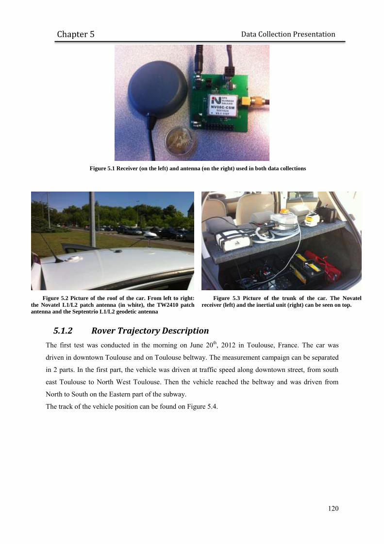
120
Data Collection Presentation
Chapter 5
Figure 5.1 Receiver (on the left) and antenna (on the right) used in both data collections
Figure 5.2 Picture of the roof of the car. From left to right:
the Novatel L1/L2 patch antenna (in white), the TW2410 patch
antenna and the Septentrio L1/L2 geodetic antenna
Figure 5.3 Picture of the trunk of the car. The Novatel
receiver (left) and the inertial unit (right) can be seen on top.
5.1.2 Rover Trajectory Description
The first test was conducted in the morning on June 20th, 2012 in Toulouse, France. The car was
driven in downtown Toulouse and on Toulouse beltway. The measurement campaign can be separated
in 2 parts. In the first part, the vehicle was driven at traffic speed along downtown street, from south
east Toulouse to North West Toulouse. Then the vehicle reached the beltway and was driven from
North to South on the Eastern part of the subway.
The track of the vehicle position can be found on Figure 5.4.

121
Data Collection Presentation
Chapter 5
Figure 5.4 Test 1 trajectory. Urban environment is indicated in blue and beltway environment is indicated in
green. Tiles Courtesy of MapQuest © OpenStreetMap contributors
Different pictures from Google StreetView can be found on Figure 5.5 to illustrate the typical
environment during the test.

122
Data Collection Presentation
Chapter 5
Figure 5.5 Example of urban (up) and beltway (down) environment driven through during the data collection.
The location of the different picture is indicated by the Google StreetView® yellow icon on the map ©Google.
Traffic was quite smooth in both urban and semi-urban environments. The data collection was
separated in 3 phases, as seen on Figure 5.6.
Figure 5.6 Phases of the data collection
The total data collection, including 7 minutes in a static position at the beginning of the test, lasted one
hour. 32 minutes data were collected in urban environment while 17 minutes data were collected on
Toulouse’s beltway.
It is important to denote that the statistics derived in the following sections are estimated only for the
urban phase and the beltway phase. As the entire data set was processed including the static phase, the
positioning performance at the beginning of the urban phase benefits from the static initialization.

123
Data Collection Presentation
Chapter 5
5.1.3 Reference Trajectory Generation
The reference trajectory was obtained by post-processing both IMU and GPS L1/L2 data from the
Novatel SPAN module. Data was post-processed using Inertial Explorer 8.40, in tight integration
mode and using multi-pass processing. The reference station used was TLSE, from the RGP network.
Due to severe signal blockages experienced during the measurement campaign, the reference
trajectory cannot be expected to be at centimeter-level at all time, even in post-processing mode. The
estimated standard deviation of the reference trajectory is plotted on Figure 5.7 and Figure 5.8, for the
urban and the beltway case. Unfortunately, only diagonal variances in XYZ coordinates were saved so
the standard deviation couldn’t be transformed in local frame. Epochs when carrier phase ambiguities
were fixed were not saved also, but they can be deduced from the estimated standard deviation
amplitude. Indeed, standard deviation amplitude should not exceed a few centimeters if carrier phase
ambiguities were fixed. It can be seen that carrier phase ambiguities are rarely fixed in urban
environment, even in post processing mode. It can be explained by the fact that the reference receiver
was tracking only GPS satellites. On the beltway, the estimated standard deviation increases
occasionally, certainly indicating a loss of tracking due to bridges.
Although the estimated standard deviation is only formal error, it can be generally expected that sub-
decimeter level accuracy on the beltway and sub-meter level accuracy in most severe urban canyon
can be expected.
Figure 5.7 Position estimated standard deviation (1 sigma) in
the XYZ coordinate frame of the reference trajectory, in downtown
Toulouse (data set 1).
Figure 5.8 Position estimated standard deviation (1
sigma) in the XYZ coordinate frame of the reference
trajectory, Toulouse’s beltway (data set 1).
Moreover as the NVS receiver was placed on another part of the vehicle roof, the lever-arm between
the reference antenna and the TW2410 was measured. Then the reference solution was corrected to
obtain a trajectory relative to the TW2410 physical center. Therefore, although the lever arm between
the SPAN antenna and the TW2410 antenna was measured carefully, errors of a few centimeters can
09:15 09:20 09:25 09:30 09:35 09:400
0.1
0.2
0.3
0.4
0.5
0.6
Estimated error standard deviaton of the reference solution (Downtown Toulouse)
Time of Day (hours:minutes)
mete
rs
sigma X
sigma Y
sigma Z
09:45 09:50 09:550
0.1
0.2
0.3
0.4
0.5
0.6
Estimated error standard deviaton of the reference solution (Toulouse's beltway)
Time of Day (hours:minutes)
mete
rs
sigma X
sigma Y
sigma Z
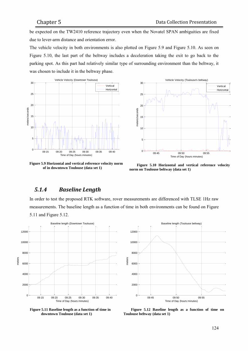
124
Data Collection Presentation
Chapter 5
be expected on the TW2410 reference trajectory even when the Novatel SPAN ambiguities are fixed
due to lever-arm distance and orientation error.
The vehicle velocity in both environments is also plotted on Figure 5.9 and Figure 5.10. As seen on
Figure 5.10, the last part of the beltway includes a deceleration taking the exit to go back to the
parking spot. As this part had relatively similar type of surrounding environment than the beltway, it
was chosen to include it in the beltway phase.
Figure 5.9 Horizontal and vertical reference velocity norm
of in downtown Toulouse (data set 1)
Figure 5.10 Horizontal and vertical reference velocity
norm on Toulouse beltway (data set 1)
5.1.4 Baseline Length
In order to test the proposed RTK software, rover measurements are differenced with TLSE 1Hz raw
measurements. The baseline length as a function of time in both environments can be found on Figure
5.11 and Figure 5.12.
Figure 5.11 Baseline length as a function of time in
downtown Toulouse (data set 1)
Figure 5.12 Baseline length as a function of time on
Toulouse beltway (data set 1)
09:15 09:20 09:25 09:30 09:35 09:400
5
10
15
20
25
30Vehicle Velocity (Downtown Toulouse)
Time of Day (hours:minutes)
mete
rs/s
econds
Vertical
Horizontal
09:45 09:50 09:550
5
10
15
20
25
30Vehicle Velocity (Toulouse's beltway)
Time of Day (hours:minutes)
mete
rs/s
econds
Vertical
Horizontal
09:15 09:20 09:25 09:30 09:35 09:400
2000
4000
6000
8000
10000
12000
Baseline length (Downtown Toulouse)
Time of Day (hours:minutes)
mete
rs
09:45 09:50 09:550
2000
4000
6000
8000
10000
12000
Baseline length (Toulouse beltway)
Time of Day (hours:minutes)
mete
rs

125
Data Collection Presentation
Chapter 5
It can be seen that the baseline length exceed 10 kilometers for the beltway part of the data set.
Therefore, atmospheric differential delays may not be negligible in single-frequency RTK, even if the
ionosphere was not particularly active on that day.
5.1.5 Measurement Availability Statistics
As in section 2.4.1, availability of the different measurements was analyzed, for the NVS receiver and
the Septentrio receiver, in both environments. An interesting fact is that the NVS receiver always
provides a code and Doppler measurement of satellites with positive elevation angle. In order to
illustrate this, the number of tracked pseudoranges in downtown Toulouse is plotted on Figure 5.13
and Figure 5.14. It can be seen that this number does not vary in the case of the NVS receiver.
Figure 5.13 Number of pseudoranges available from
Septentrio AsteRx3 in downtown Toulouse (data set1). No
elevation or C/N0 value mask is applied.
Figure 5.14 Number of pseudoranges available from
NVS-08C in downtown Toulouse (data set1). No elevation or
C/N0 value mask is applied.
However, some measurements are associated to very low C/N0 values. Therefore, the use of
measurement selection methods is particularly indicated in the case of the NVS receiver. Table 5.1 Availability statistics of NVS receiver in the first data set. No mask is applied
Downtown Toulouse Toulouse's beltway
GP
S-o
nly
Visible satellites C1 D1 L1 C1 D1 L1
at least 4 satellites 100.0% 100.0% 71.7% 100.0% 100.0% 86.5%
at least 5 satellites 100.0% 100.0% 63.2% 100.0% 100.0% 83.1%
at least 6 satellites 100.0% 100.0% 53.3% 100.0% 100.0% 77.8%
at least 7 satellites 100.0% 100.0% 40.9% 100.0% 100.0% 72.0%
at least 8 satellites 100.0% 100.0% 26.2% 100.0% 100.0% 61.5%
GP
S+G
LO
NA
SS at least 4 satellites 100.0% 100.0% 85.4% 100.0% 100.0% 91.3%
at least 5 satellites 100.0% 100.0% 80.3% 100.0% 100.0% 90.0%
at least 6 satellites 100.0% 100.0% 75.5% 100.0% 100.0% 87.9%
09:15 09:20 09:25 09:30 09:35 09:400
2
4
6
8
10
12
14
16
18
20
Satellite visibility in urban environment (AsteRx3 receiver)
Time of Day (hours:minutes)
Num
ber
of
vis
ible
pseudora
nges
GPS+GLONASS
GPS-only
09:15 09:20 09:25 09:30 09:35 09:400
2
4
6
8
10
12
14
16
18
20
Satellite visibility in urban environment (NVS receiver)
Time of Day (hours:minutes)
Num
ber
of
vis
ible
pseudora
nges
GPS+GLONASS
GPS-only

126
Data Collection Presentation
Chapter 5
at least 7 satellites 100.0% 100.0% 70.7% 100.0% 100.0% 85.7%
at least 8 satellites 100.0% 100.0% 65.1% 100.0% 100.0% 83.3%
Table 5.2 Availability statistics of AsteRx3 receiver in the first data set. No mask is applied
Downtown Toulouse Toulouse's beltway
GP
S-o
nly
Visible satellites C1 D1 L1 C1 D1 L1
at least 4 satellites 98.1% 98.1% 80.9% 98.5% 98.5% 87.5%
at least 5 satellites 93.9% 93.9% 70.2% 98.3% 98.3% 85.4%
at least 6 satellites 83.0% 83.0% 57.6% 98.1% 98.1% 83.1%
at least 7 satellites 64.6% 64.6% 39.7% 97.1% 97.1% 78.7%
at least 8 satellites 29.6% 29.6% 16.8% 95.1% 95.1% 67.1%
GP
S+G
LON
ASS
at least 4 satellites 99.9% 99.9% 99.5% 99.6% 99.6% 95.7%
at least 5 satellites 99.9% 99.9% 97.0% 99.4% 99.4% 95.0%
at least 6 satellites 99.6% 99.6% 90.9% 99.0% 99.0% 94.1%
at least 7 satellites 98.5% 98.5% 84.3% 98.7% 98.7% 92.1%
at least 8 satellites 95.4% 95.4% 77.6% 98.3% 98.3% 90.4%
The availability of at least 4 or 5 carrier phase measurements was found to be particularly high on the
AsteRx3 receiver, over 95% in both environments. Surprisingly, the availability of 4 and 5 carrier
phase measurements was higher in downtown environment than on the beltway for the AsteRx3. This
might be explained by the fact that complete signal masking occurs more often on the beltway than in
urban environment, due to bridges and tunnels. The availability of at least 4, 5 or 6 GPS-only carrier
phase measurements was found to be better on the AsteRx3 receiver, whereas the availability of at
least 7 or 8 GPS-only carrier phase measurements is better on the NVS receiver. This tends to indicate
that the AsteRx3 has a better PLL sensitivity in difficult conditions, when the vehicle undergoes high
signal masking. Moreover, the availability of GPS+GLONASS carrier phase measurements was found
to be systematically better with the AsteRx3 in the tested range of minimum number of visible
satellites. Although the uBlox PLL was found to be more sensitive than the PolaRx2 PLL in 2.5.2.1,
this result is not surprising as high sensitivity receiver manufacturers usually focus on code tracking
sensitivity rather than on carrier phase tracking sensitivity. As explained in 3.3, the proposed cycle slip
resolution technique requires at least 5 time-differenced carrier phase measurements to estimate the
cycle slip as an integer. The availability percentage of at least 5 carrier phase measurements is then an
upper bound of the cycle slip resolution module availability. It can be seen that it is quite good even in
urban environment, as it reaches 80% with GPS/GLONASS satellites on the NVS receiver.
The impact of adding GLONASS measurements is very clear as it significantly improves availability
statistics in both environments on the AsteRx3.

127
Data Collection Presentation
Chapter 5
The number of carrier phase measurements of the NVS receiver is also plotted on Figure 5.15 and
Figure 5.16.
Figure 5.15 Number of carrier phase measurements available
from NVS receiver in downtown Toulouse (data set1). No elevation
or C/N0 value mask is applied.
Figure 5.16 Number of carrier phase measurements
available from NVS receiver Toulouse’s beltway (data set1).
No elevation or C/N0 value mask is applied.
It can be seen that although the number of tracked carrier phase measurements is generally very high
on the beltway, it frequently drops down to very low value. This is due to the frequent bridges along
the beltway. However, the duration of the tracking loss is very short, as indicated on Figure 5.17.
Figure 5.17 Estimated cumulative density function of the duration of the time interval with less than 5 available
GPS/GLONASS carrier phase measurements on the NVS receiver in the 2 studied environments (data set 1).
Figure 5.17 is a plot of cumulative density function of the duration of the time interval with less than
5 available carrier phase measurements. It can be seen that most carrier phase unavailability lasts only
of a few seconds on Toulouse’s beltway, whereas they can reach tens of seconds in downtown
Toulouse. Therefore, even with GPS/GLONASS measurements, availability of carrier phase
measurements is an issue in urban environment.
09:15 09:20 09:25 09:30 09:35 09:400
2
4
6
8
10
12
14
16
18
20
Downtown Toulouse (NVS receiver)
Time of Day (hours:minutes)
Num
ber
of
vis
ible
carr
ier
phase m
easure
ments
(L1)
GPS+GLONASS
GPS-only
09:45 09:50 09:550
2
4
6
8
10
12
14
16
18
20
Toulouse's beltway (NVS receiver)
Time of Day (hours:minutes)
Num
ber
of
vis
ible
carr
ier
phase m
easure
ments
(L1)
GPS+GLONASS
GPS-only
0 5 10 15 20 25 30 35 40 45 500
0.1
0.2
0.3
0.4
0.5
0.6
0.7
0.8
0.9
1
Seconds
Cum
ula
tive d
istr
ibution f
unction
Downtown Toulouse
Toulouse's beltway
128
Data Collection Presentation
Chapter 5
5.1.6 Real-time Positioning Performance of Receivers
In this sub-chapter, real-time performances of different receivers during the 2 tests are presented. The
point is not to compare the implemented software with different softwares from the industry. Indeed
only default settings from these receivers were used and it would not be fair to confront them with the
proposed RTK software that was tuned to cope with constrained environments. The point here is
simply to show that the environments tested were difficult and that basic settings were not sufficient to
obtain the best performance possible.
Solutions will be compared based on 5 values:
The horizontal position error 68th, 95th and 99th percentiles. The horizontal position error is
computed as such:
√
(5.1)
Where:
o is the horizontal position error
o and are the errors in the local frame “North, East,Up”
As the proposed algorithm typically targets road users, results will be compared based on
horizontal error only. Indeed the vertical component is usually of lower importance in land
vehicle applications.
The fix rate. The fix rate is defined as the number of epochs during which ambiguities are
fixed as integers over the total number of epochs
The wrong fix rate. The wrong fix rate is theoretically the number of epochs with
ambiguities fixed to a wrong integer over the number of fixed ambiguities. In practice the
wrong fix rate requires to compare the obtained solution with a centimeter-level reference
solution. As it was shown in 5.1.3. that the reference trajectory could not be considered to
have such a level of precision, a new definition is adopted. In this thesis, an ambiguity
vector is declared wrongly fixed if the distance between the associated estimated position
and the reference trajectory exceeds 50 centimeters in the horizontal plan. It is an
optimistic definition for semi-urban environment but a reasonable assumption in urban
environment considering the accuracy of the reference trajectory discussed in 5.1.3 and
5.2.3.
5.1.6.1 GPS/GLONASS L1/L2 AsteRx3 Performance in Single-Point mode
Raw NMEA data were collected during Test 1. A position was computed using GPS/GLONASS
L1/L2 measurements and SBAS corrections. Results in Toulouse downtown and on Toulouse beltway
can be found on Figure 5.18 and Figure 5.19.

129
Data Collection Presentation
Chapter 5
Figure 5.18 Performance of AsteRx3 single-point real-time
algorithm (GPS/GLONASS L1/L2 +SBAS corrections), obtained
from nmea stream collection in urban environment.
Figure 5.19 Performance of AsteRx3 single-point real-
time algorithm (GPS/GLONASS L1/L2 +SBAS corrections),
obtained from nmea stream collection on Toulouse beltway.
The effect of multipath and reduced satellite geometry can clearly be seen in urban environment. The
trajectory is not smoothed and the error frequently reaches an amplitude of 5 meters amplitude in the 3
components.
On the other hand, the performance of the AsteRx3 on the beltway is very good and error is at the
sub-meter level most of the time, except when signals are shadowed by a bridge or a tunnel. Table 5.3 Performance summary of AsteRx3 in Single-Point mode, tracking GPS/GLONASS/SBAS satellites
horizontal position error
68th percentile 95th percentile 99th percentile Fix rate Wrong Fix rate
Data Set 1 1.07 meters 4.14 meters 16.02 meters - -
urban 1.36 meters 5.08 meters 18.08 meters - -
Beltway 0.94 meters 1.21 meters 2.05 meters - -
5.1.6.2 GPS/GLONASS L1 Instantaneous RTK mode Performance with
NVS-08C
The NVS-08C chip used in this data collection was soldered in such way that raw measurements and
position stream couldn’t be collected at the same time. Therefore, the performance of the positioning
software inside the chip cannot be analyzed. However, measurements were analyzed using RTKLIB.
The version used is RTKLIB v2.4.1. A pseudo real-time solution was computed using the “forward”
option, in kinematic mode. GPS/GLONASS measurements were used, while GLONASS integer
ambiguity resolution was disabled. Instantaneous ambiguity resolution was chosen. Vertical
acceleration process noise was also reduced to constrain the estimated vertical dynamic of vehicle.
Details on the configuration of RTKLIB can be found in Appendix C. As explained earlier, the
reference station used was TLSE from the RGP network.
09:15 09:20 09:25 09:30 09:35 09:40-10
-8
-6
-4
-2
0
2
4
6
8
10Error of the position estimated by AsteRx3 (Single-Point mode) in downtown Toulouse (Test 1)
Time of Day (hours:minutes)
mete
rs
Up
East
North
09:45 09:50 09:55-10
-8
-6
-4
-2
0
2
4
6
8
10Error of the position estimated by AsteRx3 (Single-Point mode) on Toulouse Beltway (Test 1)
Time of Day (hours:minutes)
mete
rs
Up
East
North

130
Data Collection Presentation
Chapter 5
Positioning error results for downtown Toulouse and Toulouse beltway can be found on Figure 5.20
and Figure 5.21 respectively.
One of the main issues underlined by these results is the low availability of the position in urban
environment using RTKLIB. Indeed, when an outlier is detected, the software doesn’t try to isolate it
and remove it, but simply discards the epoch and switches to the next epoch.
Figure 5.20 Performance of RTKLib with NVS-08C
measurements (GPS/GLONASS) in single-epoch RTK mode in
urban environment. Black asterisk represents epochs when GPS
ambiguities are fixed as integer.
Figure 5.21 Performance of RTKLib with NVS-08C
measurements (GPS/GLONASS) in single-epoch RTK mode
on Toulouse beltway. Black asterisk represents epochs when
GPS ambiguities are fixed as integer.
Moreover, the trajectory is not smoothed even on Toulouse beltway. Indeed instantaneous ambiguity
resolution is used and continuity of carrier phase ambiguities is not used in the Kalman filter. If
continuous ambiguity resolution is chosen, as on Figure 5.22 and Figure 5.23, the estimated trajectory
tends to converge toward the true solution. However, availability is still very low, while large spikes
affect the final solution. In both types of processing, ambiguity resolution is very unreliable as at least
half of the fixes are wrongly fixed. The position is however significantly smoother using continuous
ambiguity resolution, although the 95th percentile horizontal position error is over 2 meters in both
environments as seen in Table 5.4.
09:15 09:20 09:25 09:30 09:35 09:40-10
-8
-6
-4
-2
0
2
4
6
8
10
Time of Day (hours:minutes)
mete
rs
Up
East
North
Fix
09:45 09:50 09:55-10
-8
-6
-4
-2
0
2
4
6
8
10
Time of Day (hours:minutes)
mete
rs
Up
East
North
Fix

131
Data Collection Presentation
Chapter 5
Figure 5.22 Performance of RTKLIB with NVS-08C
measurements (GPS/GLONASS) in single-epoch RTK mode in
urban environment. Black asterisk represents epochs when GPS
ambiguities are fixed as integer.
Figure 5.23 Performance of RTKLIB with NVS-08C
measurements (GPS/GLONASS) in single-epoch RTK mode
on Toulouse beltway. Black asterisk represents epochs when
GPS ambiguities are fixed as integer.
Table 5.4 Performance summary of the NVS receiver using RTKLIB 2.4.1 in instantaneous and continuous RTK.
GPS/GLONASS measurements are processed
horizontal position error
68th
percentile 95th
percentile 99th
percentile Fix rate Wrong Fix rate
Inst
anta
neo
us
AR
Data Set 1 1.61 meters 9.10 meters 16.14 meters 8.4% 79.4%
Urban 3.11 meters 10.81 meters 18.87 meters 9.3% 82.0%
Beltway 1.03 meters 3.31 meters 8.66 meters 6.8% 72.9%
Co
nti
nu
ou
s A
R
Data Set 1 1.02 meters 7.65 meters 10.89 meters 6.2% 55.0%
Urban 2.05 meters 9.42 meters 12.23 meters 7.0% 57.5%
Beltway 0.79 meters 2.22 meters 6.82 meters 4.6% 47.9%
5.2 Presentation of the Second Data Collection
5.2.1 Equipment Description
A second data collection was performed on June 3rd, 2012. The same NVS receiver and TW2410 patch
antenna were used than in the first data collection. However, this time the antenna was not mounted
directly on the roof of the vehicle. Indeed, the roof of the test vehicle was congested and sticking the
antenna directly on the roof would have caused signal masking due to close environment. Therefore, it
was placed on a small metallic plan attached to the roof of the car, about 5 centimeters above the roof
09:15 09:20 09:25 09:30 09:35 09:40-10
-8
-6
-4
-2
0
2
4
6
8
10
Time of Day (hours:minutes)
mete
rs
Up
East
North
Fix
09:45 09:50 09:55-10
-8
-6
-4
-2
0
2
4
6
8
10
Time of Day (hours:minutes)
mete
rs
Up
East
North
Fix
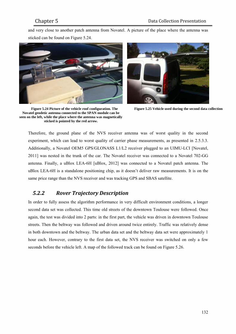
132
Data Collection Presentation
Chapter 5
and very close to another patch antenna from Novatel. A picture of the place where the antenna was
sticked can be found on Figure 5.24.
Figure 5.24 Picture of the vehicle roof configuration. The
Novatel geodetic antenna connected to the SPAN module can be
seen on the left, while the place where the antenna was magnetically
sticked is pointed by the red arrow.
Figure 5.25 Vehicle used during the second data collection
Therefore, the ground plane of the NVS receiver antenna was of worst quality in the second
experiment, which can lead to worst quality of carrier phase measurements, as presented in 2.5.3.3.
Additionally, a Novatel OEM5 GPS/GLONASS L1/L2 receiver plugged to an UIMU-LCI [Novatel,
2011] was nested in the trunk of the car. The Novatel receiver was connected to a Novatel 702-GG
antenna. Finally, a uBlox LEA-6H [uBlox, 2012] was connected to a Novatel patch antenna. The
uBlox LEA-6H is a standalone positioning chip, as it doesn’t deliver raw measurements. It is on the
same price range than the NVS receiver and was tracking GPS and SBAS satellite.
5.2.2 Rover Trajectory Description
In order to fully assess the algorithm performance in very difficult environment conditions, a longer
second data set was collected. This time old streets of the downtown Toulouse were followed. Once
again, the test was divided into 2 parts: in the first part, the vehicle was driven in downtown Toulouse
streets. Then the beltway was followed and driven around twice entirely. Traffic was relatively dense
in both downtown and the beltway. The urban data set and the beltway data set were approximately 1
hour each. However, contrary to the first data set, the NVS receiver was switched on only a few
seconds before the vehicle left. A map of the followed track can be found on Figure 5.26.
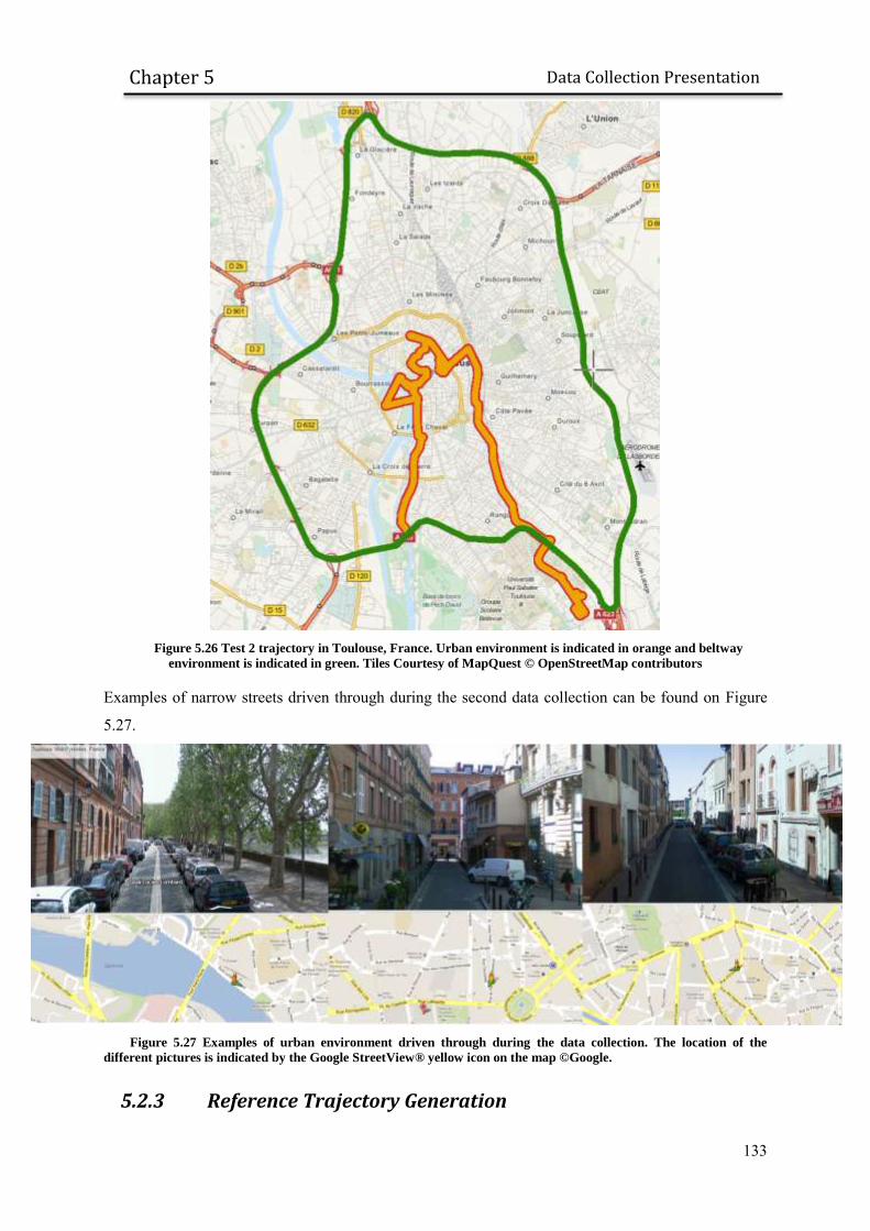
133
Data Collection Presentation
Chapter 5
Figure 5.26 Test 2 trajectory in Toulouse, France. Urban environment is indicated in orange and beltway
environment is indicated in green. Tiles Courtesy of MapQuest © OpenStreetMap contributors
Examples of narrow streets driven through during the second data collection can be found on Figure
5.27.
Figure 5.27 Examples of urban environment driven through during the data collection. The location of the
different pictures is indicated by the Google StreetView® yellow icon on the map ©Google.
5.2.3 Reference Trajectory Generation

134
Data Collection Presentation
Chapter 5
Similarly to the first data set, the reference trajectory was obtained by post-processing both IMU and
GPS L1/L2 data from the Novatel SPAN module. Data was post-processed using Inertial Explorer
8.40, in tight integration mode and using multi-pass processing. Once again, reference station used
was TLSE, from the RGP network. The estimated standard deviation of the reference trajectory is
plotted on Figure 5.7 and Figure 5.8, for the urban and the beltway case.
Figure 5.28 Position estimated standard deviation (1 sigma) in
the XYZ coordinate frame of the reference trajectory, in downtown
Toulouse (data set 2). Black asterisk represents epochs when the
reference solution indicates ambiguities have been fixed as integer.
Fix rate is equal to 24.1%
Figure 5.29 Position estimated standard deviation (1
sigma) in the XYZ coordinate frame of the reference
trajectory, Toulouse’s beltway (data set 2). Black asterisk
represents epochs when the reference solution indicates
ambiguities have been fixed as integer. Fix rate is equal to
72.0%
It can be deduced from the high estimated standard deviation of the reference trajectory that the urban
environment in the second data set is significantly more constrained than in the first data set. Although
GPS and GLONASS satellites are tracked by the Novatel receiver on L1 and L2, the number of fixes
of the reference solution in urban environment is also very low, close to 24%. On the beltway, the fix
rate reaches 72%. However, the high quality of the IMU allows keeping a high level of precision
between 2 ambiguity fixes.
Similarly to section 5.1.2, the lever-arm correction between the reference antenna and the TW2410
phase center introduces an additional centimeter-level error.
The vehicle velocity in both environments is then plotted on Figure 5.30 and Figure 5.31.
12:30 12:45 13:00 13:15 13:300
0.1
0.2
0.3
0.4
0.5
0.6
Estimated error standard deviaton of the reference solution (Downtown Toulouse)
Time of Day (hours:minutes)
mete
rs
sigma X
sigma Y
sigma Z
Fixed ambiguity
13:40 13:50 14:00 14:10 14:200
0.1
0.2
0.3
0.4
0.5
0.6
Estimated error standard deviaton of the reference solution (Toulouse's beltway)
Time of Day (hours:minutes)
mete
rs
sigma X
sigma Y
sigma Z
Fixed ambiguity

135
Data Collection Presentation
Chapter 5
Figure 5.30 Horizontal and vertical reference velocity norm
of in downtown Toulouse (data set 2)
Figure 5.31 Horizontal and vertical reference velocity
norm on Toulouse beltway (data set 2)
5.2.4 Baseline Length
In order to test the proposed RTK software, rover measurements are differenced with TLSE 1Hz raw
measurements. The baseline length as a function of time in both environments can be found on Figure
5.32 and Figure 5.33.
Figure 5.32 Baseline length as a function of time in downtown
Toulouse (data set 1)
Figure 5.33 Baseline length as a function of time on
Toulouse beltway (data set 1)
Similarly to the first data set, the baseline sometimes exceeds 10 kilometers, which may lead to non-
negligible differential atmospheric delays.
5.2.5 Measurement Availability Statistics
12:30 12:45 13:00 13:15 13:300
5
10
15
20
25
30Vehicle Velocity (Downtown Toulouse)
Time of Day (hours:minutes)
mete
rs/s
econds
Vertical
Horizontal
13:50 14:00 14:10 14:200
5
10
15
20
25
30Vehicle Velocity (Toulouse's beltway)
Time of Day (hours:minutes)
mete
rs/s
econds
Vertical
Horizontal
12:30 12:45 13:00 13:15 13:300
2000
4000
6000
8000
10000
12000
Baseline length (Downtown Toulouse)
Time of Day (hours:minutes)
mete
rs
13:40 13:50 14:00 14:10 14:200
2000
4000
6000
8000
10000
12000
Baseline length (Toulouse beltway)
Time of Day (hours:minutes)
mete
rs

136
Data Collection Presentation
Chapter 5
Similarly to the first data set, code, Doppler and carrier phase measurements availability were
analyzed for the NVS receiver and the Novatel receiver. Results can be found on Table 5.5 and Table
5.6.
Table 5.5 Availability statistics of NVS receiver in the first data set. No mask is applied
Downtown Toulouse Toulouse's beltway
GP
S-o
nly
Visible satellites C1 D1 L1 C1 D1 L1
at least 4 satellites 100.0% 100.0% 70.5% 100.0% 100.0% 83.6%
at least 5 satellites 100.0% 100.0% 59.1% 100.0% 100.0% 80.2%
at least 6 satellites 100.0% 100.0% 49.9% 100.0% 100.0% 76.6%
at least 7 satellites 100.0% 100.0% 40.3% 100.0% 100.0% 68.3%
at least 8 satellites 100.0% 100.0% 30.9% 100.0% 100.0% 57.8%
GP
S+G
LON
ASS
at least 4 satellites 100.0% 100.0% 86.4% 100.0% 100.0% 88.4%
at least 5 satellites 100.0% 100.0% 78.5% 100.0% 100.0% 86.4%
at least 6 satellites 100.0% 100.0% 71.3% 100.0% 100.0% 84.5%
at least 7 satellites 100.0% 100.0% 64.0% 100.0% 100.0% 82.9%
at least 8 satellites 100.0% 100.0% 57.2% 100.0% 100.0% 81.1%
Table 5.6 Availability statistics of Novatel OEM5 receiver in the first data set. No mask is applied
Downtown Toulouse Toulouse's beltway
GP
S-o
nly
Visible satellites C1 D1 L1 C1 D1 L1
at least 4 satellites 81.8% 81.8% 81.8% 92.2% 92.2% 92.2%
at least 5 satellites 70.2% 70.2% 70.2% 89.9% 89.9% 89.9%
at least 6 satellites 58.8% 58.8% 58.8% 86.1% 86.1% 86.1%
at least 7 satellites 44.8% 44.8% 44.8% 78.8% 78.8% 78.8%
at least 8 satellites 33.2% 33.2% 33.2% 71.5% 71.5% 71.5%
GP
S+G
LON
ASS
at least 4 satellites 92.9% 92.9% 92.9% 96.3% 96.3% 96.3%
at least 5 satellites 87.4% 87.4% 87.4% 95.4% 95.4% 95.4%
at least 6 satellites 81.6% 81.6% 81.6% 94.5% 94.5% 94.5%
at least 7 satellites 75.4% 75.4% 75.4% 93.0% 93.0% 93.0%
at least 8 satellites 68.6% 68.6% 68.6% 90.7% 90.7% 90.7%
It can be first noticed that the Novatel receiver has the same availability statistics for code, Doppler
and carrier phase measurements. Once again, the availability statistics of the NVS carrier phase
measurements were found to be lower than the one from the high-end receiver. However, carrier phase
availability is relatively good even in downtown environment, provided GPS and GLONASS satellites
are used. Indeed, at least 5 carrier phase measurements are available at least 78% of the time in
downtown Toulouse.

137
Data Collection Presentation
Chapter 5
As in 5.1.5, the plot of the estimated the cumulative density function of the duration of consecutive
epochs with less than 5 carrier phase measurements available is presented on Figure 5.34.
Figure 5.34 Estimated cumulative density function of the duration of the time interval with less than 5 available
GPS/GLONASS carrier phase measurements on the NVS receiver in the 2 studied environments (data set 2).
On the beltway, 90% of carrier phase severe outages are below 7 seconds while this duration reaches
25 seconds in downtown Toulouse.
5.2.6 Real-time Positioning Performance of Receivers
5.2.6.1 uBlox LEA-6H in GPS/SBAS L1 Single-Point mode
Raw NMEA data of the uBlox receiver were collected during Test 2. Results in Toulouse downtown
and on Toulouse beltway can be found on Figure 5.35 and Figure 5.36. Due to a problem during the
data collection, the uBlox was turned on only around 12:45. Therefore, it was initialized in downtown
environment. The performance is very bad in downtown area, as north and up coordinates are not even
in the 10 meters range. The tail of the horizontal error distribution reaches a hundred meters in urban
environment, as seen in Table 5.7. On the beltway, the result is slightly better, but still way above 1
meter. The error evolves relatively smoothly on the beltway, probably due to a strong filtering of the
receiver dynamic.
0 5 10 15 20 25 30 35 40 45 500
0.1
0.2
0.3
0.4
0.5
0.6
0.7
0.8
0.9
1
Seconds
Cum
ula
tive d
istr
ibution f
unction
Downtown Toulouse
Toulouse's beltway

138
Data Collection Presentation
Chapter 5
Figure 5.35 Performance of uBlox LEA-6H single-point real-
time algorithm (GPS L1 +SBAS corrections), obtained from nmea
stream collection in urban environment.
Figure 5.36 Performance of uBlox LEA-6H single-point
real-time algorithm (GPS L1 +SBAS corrections), obtained
from nmea stream collection on Toulouse beltway.
Table 5.7 Performance summary of the uBlox LEA-6H single-point positioning algorithm.
horizontal position error
68th percentile 95th percentile 99th percentile Fix rate Wrong Fix rate
Data Set 2 6.68 meters 46.96 meters 88.76 meters - -
urban 14.00 meters 67.85 meters 93.07 meters - -
Beltway 4.68 meters 7.15 meters 9.96 meters - -
5.2.6.2 Dual-frequency GPS/GLONASS Novatel Receiver
The position estimated by the Novatel receiver connected to the Novatel geodetic antenna was logged.
This position is obtained using GNSS only, i.e. GPS/GLONASS dual-frequency measurements.
Results are plotted on Figure 5.37 and Figure 5.38. Similarly to the AsteRx3 receiver, the position
error does not evolve smoothly. A possible explanation is that contrary to the uBlox LEA-6H, few
assumptions are made on the receiver dynamic in the positioning filter. In the case of the urban data
set, the position error appears clearly outside the 10 meters error range. However, results of the
Novatel receiver single-point positioning algorithm looked significantly worse than the one obtained
with AsteRx3 on the beltway, although driving through almost the same path.
12:30 12:45 13:00 13:15 13:30-10
-8
-6
-4
-2
0
2
4
6
8
10
Time of Day (Hours:Minutes)
mete
rs
Up
East
North
13:40 13:50 14:00 14:10 14:20-10
-8
-6
-4
-2
0
2
4
6
8
10
Time of Day (Hours:Minutes)
mete
rs
Up
East
North
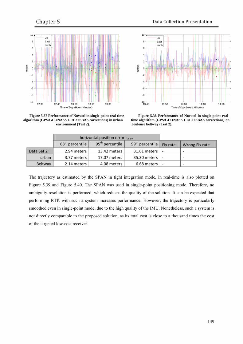
139
Data Collection Presentation
Chapter 5
Figure 5.37 Performance of Novatel in single-point real-time
algorithm (GPS/GLONASS L1/L2+SBAS corrections) in urban
environment (Test 2).
Figure 5.38 Performance of Novatel in single-point real-
time algorithm (GPS/GLONASS L1/L2+SBAS corrections) on
Toulouse beltway (Test 2).
horizontal position error
68th percentile 95th percentile 99th percentile Fix rate Wrong Fix rate
Data Set 2 2.94 meters 13.42 meters 31.61 meters - -
urban 3.77 meters 17.07 meters 35.30 meters - -
Beltway 2.14 meters 4.08 meters 6.68 meters - -
The trajectory as estimated by the SPAN in tight integration mode, in real-time is also plotted on
Figure 5.39 and Figure 5.40. The SPAN was used in single-point positioning mode. Therefore, no
ambiguity resolution is performed, which reduces the quality of the solution. It can be expected that
performing RTK with such a system increases performance. However, the trajectory is particularly
smoothed even in single-point mode, due to the high quality of the IMU. Nonetheless, such a system is
not directly comparable to the proposed solution, as its total cost is close to a thousand times the cost
of the targeted low-cost receiver.
12:30 12:45 13:00 13:15 13:30-10
-8
-6
-4
-2
0
2
4
6
8
10
Time of Day (Hours:Minutes)
mete
rs
Up
East
North
13:40 13:50 14:00 14:10 14:20-10
-8
-6
-4
-2
0
2
4
6
8
10
Time of Day (Hours:Minutes)
mete
rs
Up
East
North

140
Data Collection Presentation
Chapter 5
Figure 5.39 Performance of SPAN in single-point real-time
algorithm (GPS/GLONASS L1/L2+SBAS corrections+IMU in tight
integration mode) in urban environment (Test 2).
Figure 5.40 Performance of SPAN in single-point real-
time algorithm (GPS/GLONASS L1/L2+SBAS
corrections+IMU in tight integration mode) on Toulouse
beltway (Test 2).
horizontal position error
68th percentile 95th percentile 99th percentile Fix rate Wrong Fix rate
Data Set 2 1.00 meters 1.73 meters 2.49 meters - -
urban 1.16 meters 1.94 meters 2.75 meters - -
Beltway 0.92 meters 1.13 meters 1.26 meters - -
5.2.6.3 NVS-08C Receiver with RTKLIB (Instantaneous and Continuous
Ambiguity Resolution)
Similarly to 5.1.6.2, NVS receiver L1 GPS/GLONASS measurements were processed using RTKLIB,
in both instantaneous and continuous mode. Same configuration, given in Appendix C, is used. As
seen on Figure 5.41 to Figure 5.44, the accuracy and the availability is very poor with RTKLIB in both
modes and both environments. Trajectory is affected by very frequent discontinuities.
12:30 12:45 13:00 13:15 13:30-10
-8
-6
-4
-2
0
2
4
6
8
10
Time of Day (Hours:Minutes)
mete
rs
Up
East
North
13:40 13:50 14:00 14:10 14:20-10
-8
-6
-4
-2
0
2
4
6
8
10
Time of Day (Hours:Minutes)
mete
rs
Up
East
North

141
Data Collection Presentation
Chapter 5
Figure 5.41 Performance of RTKLIB with NVS-08C
measurements (GPS/GLONASS) in single-epoch RTK mode in
urban environment. Black asterisk represents epochs when GPS
ambiguities are fixed as integer (Test 2).
Figure 5.42 Performance of RTKLIB with NVS-08C
measurements (GPS/GLONASS) in single-epoch RTK mode
on the beltway. Black asterisk represents epochs when GPS
ambiguities are fixed as integer (Test 2).
Figure 5.43 Performance of RTKLIB with NVS-08C
measurements (GPS/GLONASS) in continuous RTK mode in urban
environment. Black asterisk represents epochs when GPS
ambiguities are fixed as integer (Test 2).
Figure 5.44 Performance of RTKLIB with NVS-08C
measurements (GPS/GLONASS) in continuous RTK mode on
the beltway. Black asterisk represents epochs when GPS
ambiguities are fixed as integer (Test 2).
Results are summarized in Table 5.8. Horizontal error 95th percentile is at least at a few meter level.
The fix rate is very low, while the wrong fix rate is very high. RTKLIB processing does not seem to be
adapted to these dynamic conditions and to both uncalibrated GLONASS measurements and multipath
contaminated measurements.
12:30 12:45 13:00 13:15 13:30-10
-8
-6
-4
-2
0
2
4
6
8
10
Time of Day (Hours:Minutes)
mete
rs
Up
East
North
Fix
13:40 13:50 14:00 14:10 14:20-10
-8
-6
-4
-2
0
2
4
6
8
10
Time of Day (Hours:Minutes)
mete
rs
Up
East
North
Fix
12:30 12:45 13:00 13:15 13:30-10
-8
-6
-4
-2
0
2
4
6
8
10
Time of Day (Hours:Minutes)
mete
rs
Up
East
North
Fix
13:40 13:50 14:00 14:10 14:20-10
-8
-6
-4
-2
0
2
4
6
8
10
Time of Day (Hours:Minutes)
mete
rs
Up
East
North
Fix
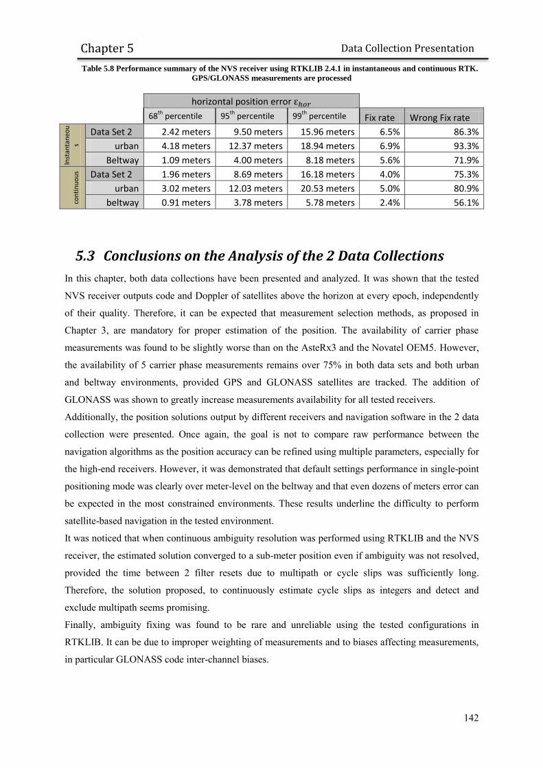
142
Data Collection Presentation
Chapter 5
Table 5.8 Performance summary of the NVS receiver using RTKLIB 2.4.1 in instantaneous and continuous RTK.
GPS/GLONASS measurements are processed
horizontal position error
68th
percentile 95th
percentile 99th
percentile Fix rate Wrong Fix rate
Inst
anta
neo
us
Data Set 2 2.42 meters 9.50 meters 15.96 meters 6.5% 86.3%
urban 4.18 meters 12.37 meters 18.94 meters 6.9% 93.3%
Beltway 1.09 meters 4.00 meters 8.18 meters 5.6% 71.9%
con
tin
uo
us Data Set 2 1.96 meters 8.69 meters 16.18 meters 4.0% 75.3%
urban 3.02 meters 12.03 meters 20.53 meters 5.0% 80.9%
beltway 0.91 meters 3.78 meters 5.78 meters 2.4% 56.1%
5.3 Conclusions on the Analysis of the 2 Data Collections
In this chapter, both data collections have been presented and analyzed. It was shown that the tested
NVS receiver outputs code and Doppler of satellites above the horizon at every epoch, independently
of their quality. Therefore, it can be expected that measurement selection methods, as proposed in
Chapter 3, are mandatory for proper estimation of the position. The availability of carrier phase
measurements was found to be slightly worse than on the AsteRx3 and the Novatel OEM5. However,
the availability of 5 carrier phase measurements remains over 75% in both data sets and both urban
and beltway environments, provided GPS and GLONASS satellites are tracked. The addition of
GLONASS was shown to greatly increase measurements availability for all tested receivers.
Additionally, the position solutions output by different receivers and navigation software in the 2 data
collection were presented. Once again, the goal is not to compare raw performance between the
navigation algorithms as the position accuracy can be refined using multiple parameters, especially for
the high-end receivers. However, it was demonstrated that default settings performance in single-point
positioning mode was clearly over meter-level on the beltway and that even dozens of meters error can
be expected in the most constrained environments. These results underline the difficulty to perform
satellite-based navigation in the tested environment.
It was noticed that when continuous ambiguity resolution was performed using RTKLIB and the NVS
receiver, the estimated solution converged to a sub-meter position even if ambiguity was not resolved,
provided the time between 2 filter resets due to multipath or cycle slips was sufficiently long.
Therefore, the solution proposed, to continuously estimate cycle slips as integers and detect and
exclude multipath seems promising.
Finally, ambiguity fixing was found to be rare and unreliable using the tested configurations in
RTKLIB. It can be due to improper weighting of measurements and to biases affecting measurements,
in particular GLONASS code inter-channel biases.

143
Tests and Results
Chapter 6
Chapter 6. Tests and Results
In this chapter, the proposed algorithm will be tested using the 2 data sets presented previously. The
performance of a basic single-epoch RTK filter will be first discussed based on the criteria defined in
section 5.1.6. This baseline solution will then be discussed based on horizontal error percentiles, fix
rate and wrong fix rate.
Then, the different propositions to improve the performance of the basic RTK filter will be added
progressively and the changes in the performance criteria values will be discussed. In particular, the
impact on performance of the following propositions will be tested:
Use of code and Doppler weighting schemes proposed in section 3.1.1 and correction of
GLONASS code biases determined in section 2.5.2.2.
Addition of the cycle slip resolution module proposed in section 3.3.
Addition of a code and Doppler multipath detection module proposed in section 3.2
Correction of GLONASS carrier phase inter-channel biases and estimation of GLONASS
ambiguities as integers, as described in section 4.2.7
Introduction of environment-dependent validation parameters, as proposed in section 4.2.6.
6.1 Proposition and Performance of a Baseline Solution
6.1.1 Baseline Solution Proposition
In order to determine the impact of each proposition, a baseline RTK filter will be added progressively
to the different proposed algorithms. The baseline filter was chosen to have the following structure:
A single-epoch ambiguity resolution RTK filter is used, as recommended in [Bahrami, et al.,
2010] for low-cost receiver. Code, Doppler and carrier phase measurements are included in a
unique filter that estimates position, velocity and acceleration together with carrier phase
ambiguities. Ambiguity state vector is re-initialized at each epoch and LAMBDA method is
used for GPS integer ambiguity resolution. GLONASS ambiguities are estimated as floats.
A minimum of 6 satellites, i.e. 5 ambiguities, is required for GPS integer ambiguity resolution
[Shirai, et al., 2011] and ambiguity is validated if the ratio test reaches 3.
No integer ambiguity is validated during the first 3 minutes of the data collection, so that all
estimated parameters, notably estimated GLONASS code biases can converge.
GLONASS code inter-channel biases are considered linear with frequency [Pratt, et al., 1998]
and estimated as such in the RTK filter.
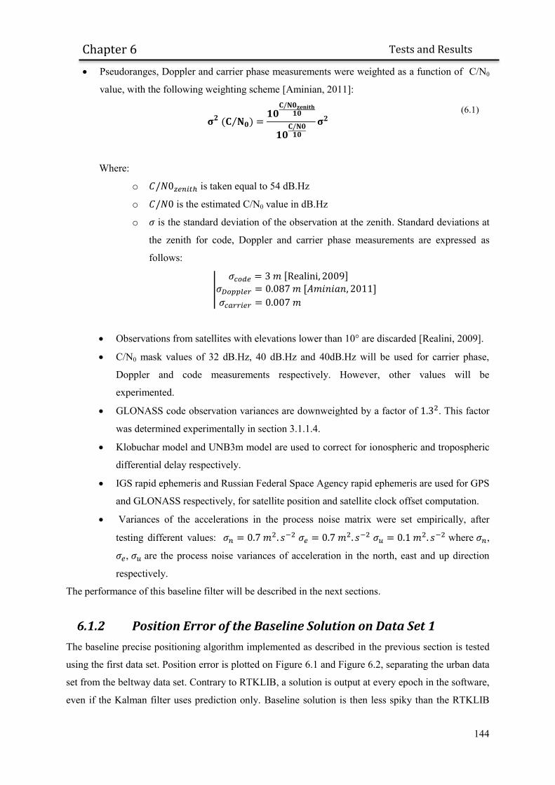
144
Tests and Results
Chapter 6
Pseudoranges, Doppler and carrier phase measurements were weighted as a function of C/N0
value, with the following weighting scheme [Aminian, 2011]:
( ⁄ )
(6.1)
Where:
o is taken equal to 54 dB.Hz
o is the estimated C/N0 value in dB.Hz
o is the standard deviation of the observation at the zenith. Standard deviations at
the zenith for code, Doppler and carrier phase measurements are expressed as
follows:
|
[ ] [ ]
Observations from satellites with elevations lower than 10° are discarded [Realini, 2009].
C/N0 mask values of 32 dB.Hz, 40 dB.Hz and 40dB.Hz will be used for carrier phase,
Doppler and code measurements respectively. However, other values will be
experimented.
GLONASS code observation variances are downweighted by a factor of . This factor
was determined experimentally in section 3.1.1.4.
Klobuchar model and UNB3m model are used to correct for ionospheric and tropospheric
differential delay respectively.
IGS rapid ephemeris and Russian Federal Space Agency rapid ephemeris are used for GPS
and GLONASS respectively, for satellite position and satellite clock offset computation.
Variances of the accelerations in the process noise matrix were set empirically, after
testing different values: where ,
, are the process noise variances of acceleration in the north, east and up direction
respectively.
The performance of this baseline filter will be described in the next sections.
6.1.2 Position Error of the Baseline Solution on Data Set 1
The baseline precise positioning algorithm implemented as described in the previous section is tested
using the first data set. Position error is plotted on Figure 6.1 and Figure 6.2, separating the urban data
set from the beltway data set. Contrary to RTKLIB, a solution is output at every epoch in the software,
even if the Kalman filter uses prediction only. Baseline solution is then less spiky than the RTKLIB

145
Tests and Results
Chapter 6
solution presented in chapter 5, as it isn’t reinitialized any time a multipath is detected. Moreover, the
null vertical velocity observation smoothed the vertical component of the solution, as shown in
Appendix D.
However, the baseline solution suffers from large biases due to code pseudorange multipath. In
particular, the performance on the first part of the beltway is poor, because it starts just after a very
challenging environment due to tree foliage.
Figure 6.1 Difference between estimated trajectory and
reference trajectory in downtown Toulouse (data set 2). Black
asterisk represents epochs when ambiguity vector is validated and
fixed as integer
Figure 6.2 Difference between estimated trajectory and
reference trajectory on Toulouse’s beltway (data set 2). Black
asterisk represents epochs when ambiguity vector is validated and
fixed as integer
Then as code measurements have a very low-weight in the processing, the bias in position is kept and
propagated through multiple epochs, even if pseudoranges observations on the beltway are in general
of very good quality, as seen in section 3.1.1.2. Therefore, simply down-weighting code measurements
in the Kalman filter is not a very efficient solution when different environments are targeted, as the
navigation will be degraded even in the period with good signal quality.
On the beltway, the speed of the vehicle is very high and the phase of the multipath changes very
quickly. As a consequence Doppler-smoothed pseudoranges tend to make the position error converge
to zero on the beltway, notably in the horizontal plane. However, this convergence is very slow.
The covariance matrix associated to the position is too optimistic relative to the actual error as shown
on Figure 6.3 and Figure 6.4. Indeed, observations multipath errors are not Gaussian and are not well
modeled by the associated covariance matrix. In some cases, the estimated variance in the vertical
direction is lower than in the horizontal direction. This is due to the weight of the null vertical velocity
constraint which depends on the speed of the vehicle, as explained in section 4.2.1.1. At high speed
such as on the beltway, this constraint has almost no effect. However when the vehicle is driven
slowly, as between 9:25 and 9:30, it plays an important role in the smoothing of the solution vertical
component.
09:15 09:20 09:25 09:30 09:35 09:40-10
-8
-6
-4
-2
0
2
4
6
8
10Error in the estimated position (Downtown Toulouse)
Time of Day (hours:minutes)
mete
rs
Up
East
North
Fix mode
09:45 09:50 09:55-10
-8
-6
-4
-2
0
2
4
6
8
10Error in the estimated position (Toulouse's beltway)
Time of Day (hours:minutes)
mete
rs
Up
East
North
Fix mode

146
Tests and Results
Chapter 6
Figure 6.3 Position estimated standard deviation (3 sigma), as
output by the Kalman filter in downtown Toulouse (data set 1).
Black asterisk represents epochs when ambiguity vector is
validated and fixed as integer
Figure 6.4 Position estimated standard deviation (3
sigma), as output by the Kalman filter on Toulouse’s beltway
(data set 1). Black asterisk represents epochs when ambiguity
vector is validated and fixed as integer
Additionally, it can be seen that even with a ratio test of 3 and a minimum of 5 ambiguities available
for ambiguity validation, wrong ambiguity fixing occurs frequently. During wrong fixes, positions are
associated to a centimeter-level estimated standard deviation in the Kalman filter, as seen on Figure
6.3 and Figure 6.4. Then, the variance associated to the position only slowly increases, indicating the
Kalman filter trusts the propagated positions deduced from the wrongly fixed ambiguities. Therefore,
wrong integer ambiguity resolution has to be avoided as much as possible.
6.1.3 Position Error of the Baseline Solution on Data Set 2
The performance of the baseline solution using the second data set is plotted on Figure 6.5 and Figure
6.6, for both urban and beltway environments.
09:15 09:20 09:25 09:30 09:35 09:40-10
-8
-6
-4
-2
0
2
4
6
8
10
Time of Day (hours:minutes)
mete
rs
3*sigma Up
3*sigma East
3*sigma North
Fix mode
09:45 09:50 09:55-10
-8
-6
-4
-2
0
2
4
6
8
10
Time of Day (hours:minutes)
mete
rs
3*sigma Up
3*sigma East
3*sigma North
Fix mode

147
Tests and Results
Chapter 6
Figure 6.5 Difference between estimated trajectory and
reference trajectory in downtown Toulouse (data set 2). Black
asterisk represents epochs when ambiguity vector is validated and
fixed as integer
Figure 6.6 Difference between estimated trajectory and
reference trajectory on Toulouse’s beltway (data set 2). Black
asterisk represents epochs when ambiguity vector is validated and
fixed as integer
Once again, the accuracy of the baseline solution in urban environment is significantly worse than on
the beltway. Large pseudorange multipath errors are propagated over multiple epochs. In the Toulouse
downtown data set, an initial convergence can be denoted. It is due to the time required for GLONASS
code bias estimates to converge. This convergence time can be reduced if these code biases are
initialized in the filter with precise initial values. It was not displayed on the first data set, as the static
initial phase was removed from the plotted data set, as explained in section 5.1.2. In the case of the
second data set, the initialization was not static and therefore was not removed.
Figure 6.7 Position estimated standard deviation in downtown
Toulouse (data set 2). Black asterisk represents epochs when
ambiguity vector is validated and fixed as integer
Figure 6.8 Position estimated standard deviation on
Toulouse’s beltway (data set 2). Black asterisk represents
epochs when ambiguity vector is validated and fixed as integer
On Toulouse beltway, the pseudorange measurements and satellite visibility are clearly better, as no
large bias can be denoted. However, the estimated position stays within 2 meters of the true position,
without converging, due to the frequent signal blockages.
12:30 12:45 13:00 13:15 13:30-10
-8
-6
-4
-2
0
2
4
6
8
10Error in the estimated position (Downtown Toulouse)
Time of Day (hours:minutes)
mete
rs
Up
East
North
Fix mode
13:40 13:50 14:00 14:10 14:20-10
-8
-6
-4
-2
0
2
4
6
8
10Error in the estimated position (Toulouse's beltway)
Time of Day (hours:minutes)
mete
rs
Up
East
North
Fix mode
12:30 12:45 13:00 13:15 13:30-10
-8
-6
-4
-2
0
2
4
6
8
10
Time of Day (hours:minutes)
mete
rs
3*sigma Up
3*sigma East
3*sigma North
Fix mode13:40 13:50 14:00 14:10 14:20
-10
-8
-6
-4
-2
0
2
4
6
8
10
Time of Day (hours:minutes)
mete
rs
3*sigma Up
3*sigma East
3*sigma North
Fix mode

148
Tests and Results
Chapter 6
Large spikes around 13:00 and 13:15 on both position error and estimated position variance plots are
due to complete or almost complete signal blockage. In these conditions, estimated position relies
almost entirely on previous vehicle dynamic behavior, which can lead to large errors. An example is
given on Figure 6.9, for the spike happening around 13:00 in downtown Toulouse.
The vehicle, coming from the top of the picture undergoes complete signal masking close to the end of
the vertical street. The Kalman filter propagated solution followed previous dynamic and does not
anticipate the 90° turn of the vehicle. However, the variance associated to the estimated position
quickly grows, as seen on Figure 6.7. Then, the estimated position quickly gets back to a better
position estimate as soon as new observations are available.
Figure 6.9 Example of Kalman filter propagation leading to large position error. Orange dots indicate estimated
position and blue dots indicate reference trajectory. The vehicle goes from the top of the picture to the bottom right
Finally, the ambiguity fixing is highly unreliable, as 80% of the fixed ambiguities are wrongly fixed in
the whole data set despite the validation process, as summarized in Table 6.1.
6.1.4 Conclusion on the Baseline Solution Performance
In this first sub-chapter, the performance of a baseline positioning filter is presented, using the 2 data
sets. Performance, characterized by horizontal position error, the fix rate and the wrong fix rate is
summarized in Table 6.1.

149
Tests and Results
Chapter 6
Table 6.1 Performance summary of the baseline solution with the 2 studied data sets
Horizontal Position Error
68th percentile 95th percentile 99th percentile Fix rate Wrong Fix rate
Data Set 1 2.18 meters 5.05 meters 6.37 meters 4.6% 89.7%
urban 2.56 meters 5.49 meters 6.50 meters 4.4% 95.2%
Beltway 1.67 meters 2.79 meters 3.50 meters 5.1% 81.1%
Data Set 2 1.84 meters 3.81 meters 6.80 meters 4.5% 80.8%
urban 2.19 meters 4.38 meters 7.94 meters 3.5% 91.8%
beltway 1.41 meters 2.21 meters 2.52 meters 6.1% 70.3%
Despite the very high C/N0 mask value, position can be heavily biased by code pseudorange multipath.
Without outlier detection technique, the estimated position can be offset during extended period of
time, while the estimated covariance matrix outputs over-optimistic estimated position variance. The
fix rate is very low and unreliable even in a semi-urban environment such as the beltway. No
significant difference in fix rate can be noticed between environments.
6.2 Improving GLONASS Code Measurement Accuracy and
Observation Covariance Matrix
In this section, GLONASS code measurements biases will be corrected using table values obtained
from an initial calibration, as performed in section 2.5.2. Secondly, code measurements will be
weighted using the weighting scheme proposed in section 3.1.1.2. This weighing scheme is
environment-dependent. Code measurements are down-weighted in urban environment, compared to
pseudoranges collected on the beltway.
6.2.1 Position Error on Data Set 1
First, the improvement brought by adding GLONASS code measurement calibration compared to the
baseline solution is plotted on Figure 6.10 and Figure 6.11.

150
Tests and Results
Chapter 6
Figure 6.10 Difference between estimated trajectory and
reference trajectory in downtown Toulouse (data set 1). Black
asterisk represents epochs when ambiguity vector is validated and
fixed as integer. Baseline configuration + GLONASS code bias
correction
Figure 6.11 Difference between estimated trajectory and
reference trajectory on Toulouse’s beltway (data set 1). Black
asterisk represents epochs when ambiguity vector is validated
and fixed as integer. Baseline configuration + GLONASS code
bias correction
The improvement brought in term of accuracy is small but visible in the horizontal position error
statistics of Table 6.3. Moreover, it can be noticed that the ambiguity has been correctly fixed on the
beltway during short period before and after 9:55, which was not the case without GLONASS code
bias correction. Indeed, large biases in GLONASS code measurements make the float ambiguity
estimates centered on wrong values, while the variances of the ambiguity estimates decrease. In that
situation, the LAMBDA method can choose the wrong integer vector as the best solution. Then if the
float value is close enough from an integer vector in the sense of the squared norm of the residuals, it
will be validated by the ratio-test, provided the residual test is small enough. Therefore, correcting
pseudoranges biases has a favorable impact on the reliability of ambiguity resolution.
In order to test the proposed weighting scheme for code and Doppler measurements, the same
configuration is kept but measurements are now weighted using the weighting schemes introduced in
chapter 3. Results can be found on Figure 6.12 and Figure 6.13.
09:15 09:20 09:25 09:30 09:35 09:40-10
-8
-6
-4
-2
0
2
4
6
8
10Error in the estimated position (Downtown Toulouse)
Time of Day (hours:minutes)
mete
rs
Up
East
North
Fix mode
09:45 09:50 09:55-10
-8
-6
-4
-2
0
2
4
6
8
10Error in the estimated position (Toulouse's beltway)
Time of Day (hours:minutes)
mete
rs
Up
East
North
Fix mode

151
Tests and Results
Chapter 6
Figure 6.12 Difference between estimated trajectory and
reference trajectory in downtown Toulouse (data set 1). Black
asterisk represents epochs when ambiguity vector is validated and
fixed as integer. Baseline configuration + GLONASS code bias
correction + proposed weighting scheme
Figure 6.13 Difference between estimated trajectory and
reference trajectory on Toulouse’s beltway (data set 1). Black
asterisk represents epochs when ambiguity vector is validated
and fixed as integer. Baseline configuration + GLONASS code
bias correction + proposed weighting scheme
The improvement brought by appropriately weighting code and Doppler measurements is significant.
It shows the importance of correctly tuning observation matrix covariance in an estimation based on
Kalman filtering. Ambiguity resolution success rate has also been improved notably on the beltway as
it reaches 47%, due to the better quality of the float solution. The number of wrong fixes in downtown
Toulouse has also been reduced to 3.3% and 50% in semi-urban and urban environment respectively.
6.2.2 Position Error on Data Set 2
Similarly to 6.2.1, the addition of GLONASS code bias correction and then of both GLONASS code
bias correction and proposed weighting scheme is tested on the second data set.
Position error obtained by simply correcting GLONASS code biases can be found on Figure 6.14 and
Figure 6.15.
09:15 09:20 09:25 09:30 09:35 09:40-10
-8
-6
-4
-2
0
2
4
6
8
10Error in the estimated position (Downtown Toulouse)
Time of Day (hours:minutes)
mete
rs
Up
East
North
Fix mode
09:45 09:50 09:55-10
-8
-6
-4
-2
0
2
4
6
8
10Error in the estimated position (Toulouse's beltway)
Time of Day (hours:minutes)
mete
rs
Up
East
North
Fix mode

152
Tests and Results
Chapter 6
Figure 6.14 Difference between estimated trajectory and
reference trajectory in downtown Toulouse (data set 2). Black
asterisk represents epochs when ambiguity vector is validated and
fixed as integer. Baseline configuration + GLONASS code bias
correction
Figure 6.15 Difference between estimated trajectory and
reference trajectory on Toulouse’s beltway (data set 2). Black
asterisk represents epochs when ambiguity vector is validated
and fixed as integer. Baseline configuration + GLONASS code
bias correction
Once again, the improvement in terms of position accuracy is small. However, these biases correction
improves both the fix rate and the estimated position variance performance, as seen on Table 6.3.
The improvement brought by using the proposed weighting scheme is shown on Figure 6.24 and
Figure 6.9.
Figure 6.16 Difference between estimated trajectory and
reference trajectory in downtown Toulouse (data set 2). Black
asterisk represents epochs when ambiguity vector is validated and
fixed as integer. Baseline configuration + GLONASS code bias
correction + proposed weighting scheme
Figure 6.17 Difference between estimated trajectory and
reference trajectory on Toulouse’s beltway (data set 2). Black
asterisk represents epochs when ambiguity vector is validated
and fixed as integer. Baseline configuration + GLONASS code
bias correction + proposed weighting scheme
The adoption of the proposed weighting scheme has the effect of removing slowly, i.e. with variation
over a few minutes, changing effects due to code multipath. The improvement in term of position
accuracy is very clear.
However, despite the very high accuracy of the float solution on Toulouse’s beltway, the number of
fixed ambiguities is very small compared to the first data set. In order to determine the reason of the
poor ambiguity fixing rate, ambiguity validation statistics were collected and reported on Table 6.2 for
12:30 12:45 13:00 13:15 13:30-10
-8
-6
-4
-2
0
2
4
6
8
10Error in the estimated position (Downtown Toulouse)
Time of Day (hours:minutes)
mete
rs
Up
East
North
Fix mode
13:40 13:50 14:00 14:10 14:20-10
-8
-6
-4
-2
0
2
4
6
8
10Error in the estimated position (Toulouse's beltway)
Time of Day (hours:minutes)
mete
rs
Up
East
North
Fix mode
12:30 12:45 13:00 13:15 13:30-10
-8
-6
-4
-2
0
2
4
6
8
10Error in the estimated position (Downtown Toulouse)
Time of Day (hours:minutes)
mete
rs
Up
East
North
Fix mode
13:40 13:50 14:00 14:10 14:20-10
-8
-6
-4
-2
0
2
4
6
8
10Error in the estimated position (Toulouse's beltway)
Time of Day (hours:minutes)
mete
rs
Up
East
North
Fix mode

153
Tests and Results
Chapter 6
both data sets. As explained in section 4.2.6, a GPS ambiguity vector is validated and fixed if it fulfills
2 conditions: it composed of at least 5 GPS ambiguities i.e. 6 GPS satellites visible, the ratio-test
exceeds the value of 3. As explained in section 6.1.1, GLONASS ambiguities are kept as floats. Table 6.2 Statistics of GPS ambiguity validation in beltway environment, for both data sets
data set 1 beltway
data set 2 beltway
Number of epoch with at least 5 GPS ambiguities 70.8 % 67.7%
Number of epoch with at least 5 GPS ambiguities a ratio-test of at
least 3 50.2% 18.8%
As seen on Table 6.2, GPS carrier phase availability is similar in both data collections. However,
ambiguity validation fails in the second data set due to the ratio-test. It indicates that the distance
between the float ambiguity vector and the closest integer vector is too important. The poor success
rate of the ratio-test can be due to both code multipath or carrier phase biases such as residual
atmospheric delay or carrier phase multipath. However, considering the high accuracy of the position
obtained on Figure 6.17, the most probable reason is carrier phase biases. The time of the day of the
second data set is closer to the daily ionospheric peak and the baseline can exceed 10 km during
several epochs. In these conditions, ionospheric differential biases can reach a few centimeters and
jeopardize ambiguity resolution. The distribution of epochs with fixed ambiguity as a function of the
baseline length with the 2 beltway data sets can be found on Figure 6.18 and Figure 6.19.
It can be seen that contrary to the first data set where ambiguities are more successfully fixed when the
baseline length is short, the correlation between successful ambiguity resolution and baseline length
seems less clear in the second data set, which tend to discard the hypothesis of a low fixing rate due to
residual atmospheric delays.
Another explanation to the low ambiguity resolution success rate can be that the antenna was not
placed on a large metallic ground plane in the second experiment whereas the antenna was
magnetically sticked to the roof of the vehicle in the first data set, as explained in section 5.2.1.
Therefore, elevation-dependent biases due to larger phase center position variation and carrier phase
multipath coming from the roof of the vehicle might also be the cause of a lower fixing rate.

154
Tests and Results
Chapter 6
Figure 6.18 Ambiguity resolution status (float or fixed) as
a function of the baseline length on Toulouse beltway (data set
1).
Figure 6.19 Ambiguity resolution status (float or fixed) as a
function of the baseline length on Toulouse beltway (data set 2).
6.2.3 Conclusion on the Baseline Solution Performance
Cumulative density function values of horizontal position error, fix rate and wrong fix rate are
reported in Table 6.3 and
Table 6.4. Table 6.3 Performance summary of the impact of adding GLONASS inter-channel bias correction with the 2
studied data sets
Horizontal Position Error
68th percentile 95th percentile 99th percentile Fix rate Wrong Fix rate
Data Set 1 2.11 meters 4.73 meters 6.44 meters 9.1% 60.5%
urban 2.30 meters 5.30 meters 6.58 meters 4.7% 98.9%
Beltway 1.83 meters 2.90 meters 3.32 meters 17.2% 41.0%
Data Set 2 1.65 meters 3.69 meters 6.37 meters 6.2% 52.7%
urban 2.01 meters 4.36 meters 7.46 meters 3.0% 92.0%
beltway 1.23 meters 2.03 meters 2.24 meters 11.5% 35.4%
09:45 09:50 09:550
2000
4000
6000
8000
10000
12000
Time of Day (hours:minutes)
Baselin
e length
(m
ete
rs)
Data set 1
Fix Mode
Float Mode
13:40 13:50 14:00 14:10 14:200
2000
4000
6000
8000
10000
12000
Time of Day (hours:minutes)
Baselin
e length
(m
ete
rs)
Data set 2
Fix Mode
Float Mode
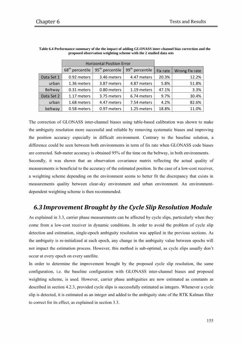
155
Tests and Results
Chapter 6
Table 6.4 Performance summary of the the impact of adding GLONASS inter-channel bias correction and the
proposed observation weighting scheme with the 2 studied data sets
Horizontal Position Error
68th percentile 95th percentile 99th percentile Fix rate Wrong Fix rate
Data Set 1 0.92 meters 3.46 meters 4.47 meters 20.3% 12.2%
urban 1.36 meters 3.87 meters 4.87 meters 5.8% 51.8%
Beltway 0.31 meters 0.80 meters 1.19 meters 47.1% 3.3%
Data Set 2 1.17 meters 3.75 meters 6.74 meters 9.7% 30.4%
urban 1.68 meters 4.47 meters 7.54 meters 4.2% 82.6%
beltway 0.58 meters 0.97 meters 1.25 meters 18.8% 11.0%
The correction of GLONASS inter-channel biases using table-based calibration was shown to make
the ambiguity resolution more successful and reliable by removing systematic biases and improving
the position accuracy especially in difficult environment. Contrary to the baseline solution, a
difference could be seen between both environments in term of fix rate when GLONASS code biases
are corrected. Sub-meter accuracy is obtained 95% of the time on the beltway, in both environments.
Secondly, it was shown that an observation covariance matrix reflecting the actual quality of
measurements is beneficial to the accuracy of the estimated position. In the case of a low-cost receiver,
a weighting scheme depending on the environment seems to better fit the discrepancy that exists in
measurements quality between clear-sky environment and urban environment. An environment-
dependent weighting scheme is then recommended.
6.3 Improvement Brought by the Cycle Slip Resolution Module
As explained in 3.3, carrier phase measurements can be affected by cycle slips, particularly when they
come from a low-cost receiver in dynamic conditions. In order to avoid the problem of cycle slip
detection and estimation, single-epoch ambiguity resolution was applied in the previous sections. As
the ambiguity is re-initialized at each epoch, any change in the ambiguity value between epochs will
not impact the estimation process. However, this method is sub-optimal, as cycle slips usually don’t
occur at every epoch on every satellite.
In order to determine the improvement brought by the proposed cycle slip resolution, the same
configuration, i.e. the baseline configuration with GLONASS inter-channel biases and proposed
weighting scheme, is used. However, carrier phase ambiguities are now estimated as constants as
described in section 4.2.3, provided cycle slips is successfully estimated as integers. Whenever a cycle
slip is detected, it is estimated as an integer and added to the ambiguity state of the RTK Kalman filter
to correct for its effect, as explained in section 3.3.

156
Tests and Results
Chapter 6
6.3.1 Position Error on Data Set 1
The new positioning error results are plotted on Figure 6.20 and Figure 6.21.
Figure 6.20 Position error in downtown Toulouse (data set 1).
Black asterisk represents epochs when ambiguity vector is validated
and fixed as integer
Figure 6.21 Position error on Toulouse’s beltway (data set 1).
Black asterisk represents epochs when ambiguity vector is validated
and fixed as integer
Position error has been reduced compared to the single-epoch approach, notably in urban environment
where the solution is smoother. Indeed, as carrier phase measurements are associated to a very small
variance, the Kalman filter tends to give them more weight while the ambiguity estimate gets more
accurate. Assuming the ambiguity is constant increases the accuracy of the float ambiguity through
time.
However, when very large multipaths are present during an extended period, position can still be
offset by a few meters. This situation is visible when the vehicle remains static during a long time in a
shadowed environment, due to traffic for instance. An example of ground track can be found on Figure
6.22, during an event occurring between 9:20 and 9:25. This event points out one of the limit of the
proposed algorithm. Estimating carrier phase as constants increases the accuracy of the float ambiguity
provided pseudorange error is zero mean over a short period of time. In the case of time-correlated
multipath in a static environment, the solution can be biased and never converge. However, as the
targeted application is a land vehicle, the environment is expected to be dynamic and the time
correlation of pseudorange multipath short.
09:15 09:20 09:25 09:30 09:35 09:40-10
-8
-6
-4
-2
0
2
4
6
8
10Error in the estimated position (Downtown Toulouse)
Time of Day (hours:minutes)
mete
rs
Up
East
North
Fix mode
09:45 09:50 09:55-10
-8
-6
-4
-2
0
2
4
6
8
10Error in the estimated position (Toulouse's beltway)
Time of Day (hours:minutes)
mete
rs
Up
East
North
Fix mode

157
Tests and Results
Chapter 6
Figure 6.22 Example of drifting position due to high multipath during a static period, between hour 9.35 and
hour 9.40. Orange spots indicate estimated position and blue spots indicate reference trajectory.
Surprisingly the fix rate was slightly decreased from 47% to 40% on the beltway. However, it has
greatly increased the reliability of ambiguity resolution as no wrong fixes were identified on the
beltway as seen on Table 6.6.
6.3.2 Position Error on Data Set 2
Results with the second data set can be found on Figure 6.23 and Figure 6.24.

158
Tests and Results
Chapter 6
Figure 6.23 Position error in downtown Toulouse (data set 2).
Black asterisk represents epochs when ambiguity vector is validated
and fixed as integer
Figure 6.24 Position error on Toulouse’s beltway (data set 2).
Black asterisk represents epochs when ambiguity vector is validated
and fixed as integer
Once again, the improvement is clear in both environments. The number of fixed ambiguity has been
improved on the beltway while the wrong fix rate has decreased in both environments.
On the beltway epochs with fixed ambiguities are more “packed” together compared to the baseline
solution. It is due to the fact that an ambiguity is maintained fixed as long as the cycle slip resolution
module validates estimated integer cycle slips or has enough observations to estimate the cycle slip
vector.
6.3.3 Conclusion on the Impact of the Cycle Slip Resolution Module
Performances improvements brought by cycle slip resolution module are summarized in Table 6.5. Table 6.5 Performance summary of the baseline solution improved by GLONASS code inter-channel bias
correction, the proposed observation weighting scheme and the cycle slip resolution module with the 2 studied data
sets
Horizontal Position Error
68th percentile 95th percentile 99th percentile Fix rate Wrong Fix rate
Data Set 1 0.99 meters 3.21 meters 4.28 meters 15.6% 6.5%
urban 1.25 meters 3.65 meters 4.64 meters 2.5% 63.8%
Beltway 0.28 meters 0.67 meters 1.20 meters 39.9% 0.0%
Data Set 2 0.98 meters 2.91 meters 4.98 meters 12.9% 13.7%
urban 1.39 meters 3.34 meters 5.54 meters 2.6% 40.3%
beltway 0.48 meters 0.89 meters 1.15 meters 29.8% 9.8%
The continuous estimation of carrier phase ambiguities thanks to the cycle slip resolution module was
shown to bring an improvement in both environments and both data sets, mostly in term of horizontal
position error and ambiguity fixing rate. Continuous ambiguity estimation has a smoothing effect on
the trajectory and improves horizontal error statistics, in all environments. Finally, continuous
ambiguity resolution was found to increase ambiguity resolution reliability. However, in a high
12:30 12:45 13:00 13:15 13:30-10
-8
-6
-4
-2
0
2
4
6
8
10Error in the estimated position (Downtown Toulouse)
Time of Day (hours:minutes)
mete
rs
Up
East
North
Fix mode
13:40 13:50 14:00 14:10 14:20-10
-8
-6
-4
-2
0
2
4
6
8
10Error in the estimated position (Toulouse's beltway)
Time of Day (hours:minutes)
mete
rs
Up
East
North
Fix mode
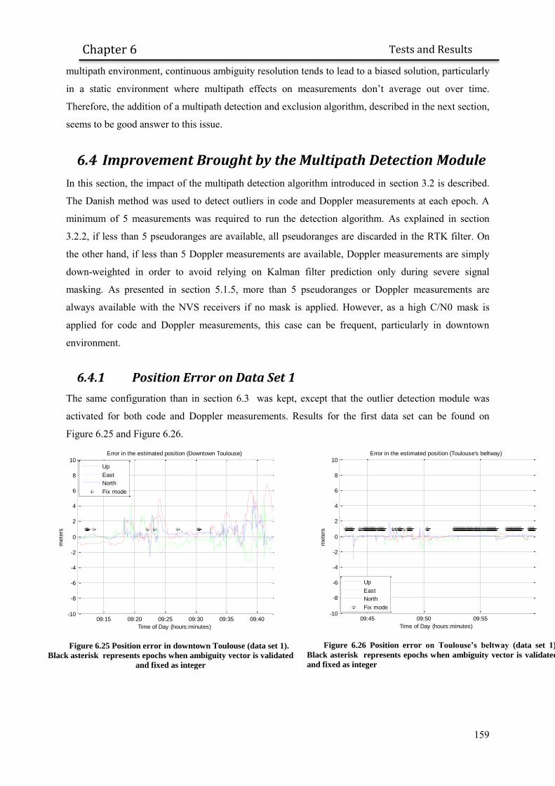
159
Tests and Results
Chapter 6
multipath environment, continuous ambiguity resolution tends to lead to a biased solution, particularly
in a static environment where multipath effects on measurements don’t average out over time.
Therefore, the addition of a multipath detection and exclusion algorithm, described in the next section,
seems to be good answer to this issue.
6.4 Improvement Brought by the Multipath Detection Module
In this section, the impact of the multipath detection algorithm introduced in section 3.2 is described.
The Danish method was used to detect outliers in code and Doppler measurements at each epoch. A
minimum of 5 measurements was required to run the detection algorithm. As explained in section
3.2.2, if less than 5 pseudoranges are available, all pseudoranges are discarded in the RTK filter. On
the other hand, if less than 5 Doppler measurements are available, Doppler measurements are simply
down-weighted in order to avoid relying on Kalman filter prediction only during severe signal
masking. As presented in section 5.1.5, more than 5 pseudoranges or Doppler measurements are
always available with the NVS receivers if no mask is applied. However, as a high C/N0 mask is
applied for code and Doppler measurements, this case can be frequent, particularly in downtown
environment.
6.4.1 Position Error on Data Set 1
The same configuration than in section 6.3 was kept, except that the outlier detection module was
activated for both code and Doppler measurements. Results for the first data set can be found on
Figure 6.25 and Figure 6.26.
Figure 6.25 Position error in downtown Toulouse (data set 1).
Black asterisk represents epochs when ambiguity vector is validated
and fixed as integer
Figure 6.26 Position error on Toulouse’s beltway (data set 1).
Black asterisk represents epochs when ambiguity vector is validated
and fixed as integer
09:15 09:20 09:25 09:30 09:35 09:40-10
-8
-6
-4
-2
0
2
4
6
8
10Error in the estimated position (Downtown Toulouse)
Time of Day (hours:minutes)
mete
rs
Up
East
North
Fix mode
09:45 09:50 09:55-10
-8
-6
-4
-2
0
2
4
6
8
10Error in the estimated position (Toulouse's beltway)
Time of Day (hours:minutes)
mete
rs
Up
East
North
Fix mode

160
Tests and Results
Chapter 6
The addition of a multipath detection module brings only a modest improvement to the solution, as
seen in Table 6.14. The horizontal position error 95th percentile on the beltway was even slightly
degraded, despite an improvement in the fix rate.
However, it is not totally fair to compare the new estimated trajectory with the solution obtained in
6.3.1 using the same C/N0 mask values. Indeed, one of the advantages of the multipath detection and
exclusion module is that it theoretically allows using lower C/N0 mask value which should improve
the geometry and potentially the accuracy of the final solution. Indeed, multipath-contaminated
measurements should be detected and excluded.
In order to determine the impact of the multipath detection and exclusion module, the data set was
processed for C/N0 mask values of 32, 36 and 40 dB.Hz for pseudoranges, Doppler and carrier phase
measurements. Solutions are compared based on the 95th percentile of the horizontal position error.
Data is processed first without the multipath detection module and then with the multipath module
activated. Results are reported in Table 6.6, Table 6.7, Table 6.8 and Table 6.9. In all these tables, the
5 lowest values are underlined in red. It can be seen that the best horizontal position error 95th
percentile is slightly improved in urban environment whereas the result is worse when the multipath
module is activated on the beltway for a pseudorange mask value of 32dB.Hz and 40 dB.Hz. In the
first case, there is probably at least 2 faulty measurements whereas in the last case, most erroneous
measurement might have been removed but the geometry is weak. Table 6.6 95th percentile value of the horizontal position error for different C/N0 mask values on Toulouse
beltway (data set 1) using the proposed weighting scheme and the cycle slip resolution module.
Pseudorange mask
32 dB.Hz 36 dB.Hz 40 dB.Hz
Doppler mask Doppler mask Doppler mask
32 dB.Hz
36 dB.Hz
40 dB.Hz
32 dB.Hz
36 dB.Hz
40 dB.Hz
32 dB.Hz
36 dB.Hz
40 dB.Hz
Car
rier
Ph
ase
Mas
k
32 dB.Hz
0.96 meters
0.96 meters
0.96 meters
0.96 meters
0.95 meters
0.98 meters
0.65 meters
0.65 meters
0.67 meters
36 dB.Hz
0.96 meters
0.80 meters
0.96 meters
0.96 meters
0.95 meters
0.98 meters
0.65 meters
0.65 meters
0.67 meters
40 dB.Hz
0.80 meters
0.80 meters
0.67 meters
0.99 meters
0.78 meters
0.68 meters
0.65 meters
0.65 meters
0.67 meters

161
Tests and Results
Chapter 6
Table 6.7 95th percentile value of the horizontal position error for different C/N0 mask values on Toulouse
beltway (data set 1) using the proposed weighting scheme, the cycle slip resolution module and the multipath detection
module
Pseudorange mask
32 dB.Hz 36 dB.Hz 40 dB.Hz
Doppler mask Doppler mask Doppler mask
32 dB.Hz
36 dB.Hz
40 dB.Hz
32 dB.Hz
36 dB.Hz
40 dB.Hz
32 dB.Hz
36 dB.Hz
40 dB.Hz
Car
rier
Ph
ase
Mas
k 32 dB.Hz
1.03 meters
1.04 meters
1.04 meters
0.81 meters
0.83 meters
0.89 meters
0.82 meters
0.83 meters
0.88 meters
36 dB.Hz
1.03 meters
1.04 meters
1.04 meters
0.89 meters
0.89 meters
0.93 meters
0.82 meters
0.83 meters
0.88 meters
40 dB.Hz
1.02 meters
0.83 meters
0.89 meters
0.81 meters
0.84 meters
0.90 meters
0.82 meters
0.83 meters
0.88 meters
Table 6.8 95th percentile value of the horizontal position error for different C/N0 mask values in downtown
Toulouse (data set 1) using the proposed weighting scheme and the cycle slip resolution module
Pseudorange mask
32 dB.Hz 36 dB.Hz 40 dB.Hz
Doppler mask Doppler mask Doppler mask
32 dB.Hz
36 dB.Hz
40 dB.Hz
32 dB.Hz
36 dB.Hz
40 dB.Hz
32 dB.Hz
36 dB.Hz
40 dB.Hz
Car
rier
Ph
ase
Mas
k 32 dB.Hz
4.89 meters
4.79 meters
4.79 meters
5.14 meters
5.15 meters
5.47 meters
3.70 meters
3.76 meters
3.65 meters
36 dB.Hz
4.90 meters
4.79 meters
4.79 meters
5.15 meters
5.14 meters
5.12 meters
3.60 meters
3.61 meters
3.63 meters
40 dB.Hz
4.93 meters
4.78 meters
4.33 meters
5.30 meters
5.17 meters
4.17 meters
3.57 meters
3.59 meters
3.61 meters
Table 6.9 95th percentile value of the horizontal position error for different C/N0 mask values in downtown
Toulouse (data set 1) using the proposed weighting scheme, the cycle slip resolution module and the multipath
detection module
Pseudorange mask
32 dB.Hz 36 dB.Hz 40 dB.Hz
Doppler mask Doppler mask Doppler mask
32 dB.Hz
36 dB.Hz
40 dB.Hz
32 dB.Hz
36 dB.Hz
40 dB.Hz
32 dB.Hz
36 dB.Hz
40 dB.Hz
Car
rier
Ph
ase
Mas
k 32 dB.Hz
4.75 meters
4.79 meters
5.00 meters
3.94 meters
3.96 meters
3.96 meters
3.37 meters
3.30 meters
3.39 meters
36 dB.Hz
4.75 meters
4.79 meters
4.98 meters
4.00 meters
4.02 meters
4.11 meters
3.38 meters
3.27 meters
3.37 meters
40 dB.Hz
5.12 meters
4.05 meters
4.07 meters
3.96 meters
3.98 meters
4.00 meters
3.37 meters
3.40 meters
3.40 meters

162
Tests and Results
Chapter 6
A second remark is that the pseudorange C/N0 mask value proposed in 6.1.1 remains relevant when
the multipath detection module is activated as it provides good results in both environments.
Moreover, it can be seen that horizontal position error is mostly impacted by the pseudorange mask.
Indeed once the pseudorange mask is chosen, the horizontal position error statistics only slightly vary
with Doppler and carrier phase mask value. The low impact of Doppler mask may be explained by the
fact that low C/N0 measurements are significantly down-weighted in the proposed weighting scheme.
Therefore the Kalman filter tends to give more weight to the speed predicted value.
The effect of the carrier phase C/N0 mask values choice is more difficult to determine. Indeed, the
choice of the code and Doppler measurements C/N0 mask is simply a trade-off between geometry
quality and measurements quality. On the other hand, the impact of the carrier phase on position
estimation depends on:
The resolution of cycle slips. The estimation of cycle slips as integers depends on both carrier
phase and Doppler measurements quality and geometry.
The resolution of the ambiguity vector as an integer
If the cycle slip cannot be estimated as an integer, i.e. the ambiguity state is re-initialized, and
ambiguity vector is not validated, carrier phase measurements bring no constraint in the position
estimation, as they are ambiguous.
6.4.2 Position Error on Data Set 2
The second data set was processed the same way than data set 1. First, the multipath detection module
was activated and data was processed with a C/N0 mask value of 32dB.Hz, 40dB.Hz and 40dB.Hz for
code, Doppler and carrier phase measurements respectively. Results are plotted on Figure 6.27 and
Figure 6.28.
Figure 6.27 Position error in downtown Toulouse (data set 2).
Black asterisk represents epochs when ambiguity vector is validated
and fixed as integer
Figure 6.28 Position error on Toulouse’s beltway (data set 2).
Black asterisk represents epochs when ambiguity vector is validated
and fixed as integer
12:30 12:45 13:00 13:15 13:30-10
-8
-6
-4
-2
0
2
4
6
8
10Error in the estimated position (Downtown Toulouse)
Time of Day (hours:minutes)
mete
rs
Up
East
North
Fix mode
13:40 13:50 14:00 14:10 14:20-10
-8
-6
-4
-2
0
2
4
6
8
10Error in the estimated position (Toulouse's beltway)
Time of Day (hours:minutes)
mete
rs
Up
East
North
Fix mode

163
Tests and Results
Chapter 6
Then, data was processed with different C/N0 mask value ranges. Table 6.10, Table 6.11, Table 6.12
and Table 6.13 summarize the 95th percentile of the horizontal position error for the different C/N0
mask values. It can be seen contrary to the first data set, the multipath detection technique improves
the performance in both environments in this data set. Best performance in urban environment with
and without the multipath module are however very similar in this data set. The best C/N0 mask value
for code pseudorange was found to be 40 dB.Hz for urban environment and 32 dB.Hz for the beltway,
processing the second data set with or without the multipath exclusion module. Once again, the
changes of the Doppler C/N0 mask value was not found to impact the performance drastically, once
the pseudorange mask value is chosen. The best performance is obtained with a Doppler mask value of
32dB.Hz when the multipath module is activated on the beltway and 40dB.Hz in urban environment.
Lastly, it can be seen that the difference between the smallest value of the 95th percentile and the
largest is significantly smaller in tables with the multipath exclusion module activated than in tables
without the multipath exclusion module.
It is interesting as it avoids the high dependency of the solution quality on the correct tuning of the
C/N0 mask values. Therefore, as the precise positioning algorithm is intended to be used in real-time
without any input from the user, the C/N0 mask can be set to an a priori value without the risk of
highly degrading the solution. Table 6.10 95th percentile value of the horizontal position error for different C/N0 mask values on Toulouse
beltway (data set 2) using the proposed weighting scheme and the cycle slip resolution module.
Pseudorange mask
32 dB.Hz 36 dB.Hz 40 dB.Hz
Doppler mask Doppler mask Doppler mask
32 dB.Hz
36 dB.Hz
40 dB.Hz
32 dB.Hz
36 dB.Hz
40 dB.Hz
32 dB.Hz
36 dB.Hz
40 dB.Hz
Car
rier
Ph
ase
Mas
k 32 dB.Hz
0.83 meters
0.88 meters
0.90 meters
0.86 meters
0.84 meters
0.90 meters
0.85 meters
0.86 meters
0.89 meters
36 dB.Hz
0.83 meters
0.88 meters
0.90 meters
0.86 meters
0.87 meters
0.90 meters
0.85 meters
0.86 meters
0.90 meters
40 dB.Hz
0.90 meters
0.91 meters
0.90 meters
0.89 meters
0.90 meters
0.90 meters
0.88 meters
0.89 meters
0.90 meters
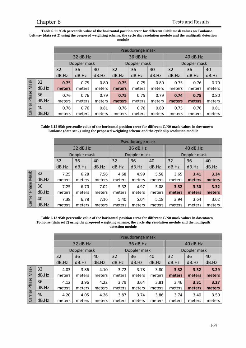
164
Tests and Results
Chapter 6
Table 6.11 95th percentile value of the horizontal position error for different C/N0 mask values on Toulouse
beltway (data set 2) using the proposed weighting scheme, the cycle slip resolution module and the multipath detection
module
Pseudorange mask
32 dB.Hz 36 dB.Hz 40 dB.Hz
Doppler mask Doppler mask Doppler mask
32 dB.Hz
36 dB.Hz
40 dB.Hz
32 dB.Hz
36 dB.Hz
40 dB.Hz
32 dB.Hz
36 dB.Hz
40 dB.Hz
Car
rier
Ph
ase
Mas
k 32 dB.Hz
0.75 meters
0.75 meters
0.80 meters
0.75 meters
0.75 meters
0.80 meters
0.75 meters
0.76 meters
0.79 meters
36 dB.Hz
0.76 meters
0.76 meters
0.79 meters
0.75 meters
0.75 meters
0.79 meters
0.74 meters
0.75 meters
0.80 meters
40 dB.Hz
0.76 meters
0.76 meters
0.81 meters
0.76 meters
0.76 meters
0.80 meters
0.75 meters
0.76 meters
0.81 meters
Table 6.12 95th percentile value of the horizontal position error for different C/N0 mask values in downtown
Toulouse (data set 2) using the proposed weighting scheme and the cycle slip resolution module
Pseudorange mask
32 dB.Hz 36 dB.Hz 40 dB.Hz
Doppler mask Doppler mask Doppler mask
32 dB.Hz
36 dB.Hz
40 dB.Hz
32 dB.Hz
36 dB.Hz
40 dB.Hz
32 dB.Hz
36 dB.Hz
40 dB.Hz
Car
rier
Ph
ase
Mas
k 32 dB.Hz
7.25 meters
6.28 meters
7.56 meters
4.68 meters
4.99 meters
5.58 meters
3.65 meters
3.41 meters
3.34 meters
36 dB.Hz
7.25 meters
6.70 meters
7.02 meters
5.32 meters
4.97 meters
5.08 meters
3.52 meters
3.30 meters
3.32 meters
40 dB.Hz
7.38 meters
6.78 meters
7.16 meters
5.40 meters
5.04 meters
5.18 meters
3.94 meters
3.64 meters
3.62 meters
Table 6.13 95th percentile value of the horizontal position error for different C/N0 mask values in downtown
Toulouse (data set 2) using the proposed weighting scheme, the cycle slip resolution module and the multipath
detection module
Pseudorange mask
32 dB.Hz 36 dB.Hz 40 dB.Hz
Doppler mask Doppler mask Doppler mask
32 dB.Hz
36 dB.Hz
40 dB.Hz
32 dB.Hz
36 dB.Hz
40 dB.Hz
32 dB.Hz
36 dB.Hz
40 dB.Hz
Car
rier
Ph
ase
Mas
k 32 dB.Hz
4.03 meters
3.86 meters
4.10 meters
3.72 meters
3.78 meters
3.80 meters
3.32 meters
3.32 meters
3.29 meters
36 dB.Hz
4.12 meters
3.96 meters
4.22 meters
3.79 meters
3.64 meters
3.81 meters
3.46 meters
3.31 meters
3.27 meters
40 dB.Hz
4.20 meters
4.05 meters
4.26 meters
3.87 meters
3.74 meters
3.86 meters
3.74 meters
3.40 meters
3.50 meters

165
Tests and Results
Chapter 6
6.4.3 Conclusion on the Impact of the Multipath Detection and
Exclusion Module
Performance of the RTK filter obtained by using the proposed observation weighting schemes,
GLONASS inter-channel code biases correction, cycle slip resolution module and multipath exclusion
module are summarized in Table 6.14. A C/N0 mask of 32dB.Hz, 40dB.Hz and 40dB.Hz for carrier
phase, Doppler and code measurements was used, as it was still found to be one of the most relevant
mask values combination for both data sets when the multipath exclusion module is activated.
However, it was shown that the pseudorange mask value had the largest impact, as Doppler and carrier
phase mask value choice only slightly changed horizontal error statistics. Table 6.14 Performance summary of the baseline solution improved by GLONASS code inter-channel bias
correction, the proposed observation weighting scheme, the cycle slip resolution module and the multipath exclusion
module with the 2 studied data sets
Horizontal Position Error
68th percentile 95th percentile 99th percentile Fix rate Wrong Fix rate
Data Set 1 0.90 meters 2.90 meters 3.84 meters 17.0% 1.4%
urban 1.25 meters 3.39 meters 4.09 meters 1.3% 29.2%
Beltway 0.37 meters 0.89 meters 1.46 meters 45.9% 0.0%
Data Set 2 0.88 meters 2.97 meters 5.56 meters 15.5% 10.8%
urban 1.32 meters 3.34 meters 6.22 meters 6.2% 26.6%
beltway 0.35 meters 0.80 meters 1.05 meters 31.1% 5.6%
In general, the multipath detection and exclusion module was found to decrease horizontal error
statistics by a few decimeters, except on the beltway in the first data set. Moreover, the fix rate gained
6% in the first data set and 1% in the second on the beltway. The wrong fix rate was decreased in both
data sets and both environments.
Finally, the use of the multipath module tend to make the horizontal position error uniform as a
function of the C/N0 mask values for pseudorange, Doppler and carrier phase measurement. The
optimal C/N0 masks are difficult to set as they were found to depend on both the environment and the
data set. Considering that mask values can greatly change the accuracy of the final solution, the use of
a multipath detection module is then recommended.
6.5 Improvement Brought by Adding Integer Resolution of
GLONASS Ambiguities
In order to fully benefit from the precision of GLONASS carrier phase measurements, GLONASS
ambiguities have to be estimated as integers. It involves 2 steps: calibrating GLONASS biases during
a static data collection in a clear-sky environment and performing the correct processing of
GLONASS ambiguities in the software in order to isolate them as integers. The first step is described

166
Tests and Results
Chapter 6
in 4.2.7.1, while the second step is described in 4.2.7.4. In this section, GLONASS carrier phase
measurements were corrected from GLONASS inter-channel biases and GPS/GLONASS combined
integer ambiguity resolution is performed. Although the receiver has been completely powered off
between the 2 data collection, the same inter-channel bias correction value of 0.47 cm for 2 adjacent
frequencies is used for both data sets.
6.5.1 Position Error on Data Set 1
The first data set was reprocessed using the proposed weighting scheme, the cycle slip resolution
module, the multipath exclusion module activated and adding GLONASS ambiguities in the integer
estimation step. The improvement is significant, as seen on Figure 6.29 and Figure 6.30.
Figure 6.29 Position error in downtown Toulouse (data set 1).
Black asterisk represents epochs when ambiguity vector is validated
and fixed as integer
Figure 6.30 Position error on Toulouse’s beltway (data set 1).
Black asterisk represents epochs when ambiguity vector is
validated and fixed as integer
The number of epochs with fixed ambiguities has been improved in both environments. The number of
wrong fixes in downtown Toulouse is also greatly reduced. The fixing statistics are presented in Table
6.15. Table 6.15 Statistics of GPS+GLONASS ambiguity validation in beltway and downtown environment, for data
set 1.
Toulouse beltway
Downtown Toulouse
Number of epoch with at least 5 GPS+GLONASS ambiguities 81.8 % 64.0%
Number of epoch with at least 5 GPS+GLONASS ambiguities a ratio-
test of at least 3 61.8% 17.0%
Comparing with Table 6.2, it can be seen that on the beltway the number of epoch with at least 5
ambiguities grows from 70.8% to 81.8% whereas the final fixing rate grows from 45.9% to 61.8%
09:15 09:20 09:25 09:30 09:35 09:40-10
-8
-6
-4
-2
0
2
4
6
8
10Error in the estimated position (Downtown Toulouse)
Time of Day (hours:minutes)
mete
rs
Up
East
North
Fix mode
09:45 09:50 09:55-10
-8
-6
-4
-2
0
2
4
6
8
10Error in the estimated position (Toulouse's beltway)
Time of Day (hours:minutes)
mete
rs
Up
East
North
Fix mode

167
Tests and Results
Chapter 6
compared to the previous experience. It shows that the improvement in the ambiguity fixing success
rate is not only due to the larger number of epochs with the minimum number of carrier phase
measurements required, but also to the improved effectiveness of the LAMBDA method and the ratio
test in finding and validating the correct integer vector due to a better geometry. However, ambiguity
are still fixed less than one fifth of the time in urban environment despite 64% availability of the
minimum number of ambiguities required. Indeed, the float solution is not accurate enough because of
code multipath and weak satellite geometry, which makes the ratio test fail.
6.5.2 Position Error on Data Set 2
In the second data set, the improvement brought by adding GLONASS ambiguities in the integer
ambiguity estimation step is also very clear, as seen on Figure 6.31 and Figure 6.32.
Figure 6.31 Position error in downtown Toulouse (data set 2).
Black asterisk represents epochs when ambiguity vector is validated
and fixed as integer
Figure 6.32 Position error on Toulouse’s beltway (data set 2).
Black asterisk represents epochs when ambiguity vector is
validated and fixed as integer
The number of epoch with fixed ambiguities grows from 22.8% to 39.7% on the beltway, as seen on
Table 6.17. Similarly to the first data set, the number of wrong fix has been greatly reduced on the
beltway to 0.1%. In urban environment, the number of wrong fixes still represents more than 11% of
the total fixes. However, considering the small number of total number of fixes, wrong integer fixing
does not greatly affect horizontal position error.
However, the fixing rate of the second data set in the beltway is still significantly lower than for the
first data set, probably due to a worst placement of the antenna as explained in 6.2.2.
12:30 12:45 13:00 13:15 13:30-10
-8
-6
-4
-2
0
2
4
6
8
10Error in the estimated position (Downtown Toulouse)
Time of Day (hours:minutes)
mete
rs
Up
East
North
Fix mode
13:40 13:50 14:00 14:10 14:20-10
-8
-6
-4
-2
0
2
4
6
8
10Error in the estimated position (Toulouse's beltway)
Time of Day (hours:minutes)
mete
rs
Up
East
North
Fix mode

168
Tests and Results
Chapter 6
Table 6.16 Statistics of GPS+GLONASS ambiguity validation in beltway and downtown environment, for data
set 2.
Toulouse beltway
Downtown Toulouse
Number of epoch with at least 5 GPS+GLONASS ambiguities 81.2 % 52.3%
Number of epoch with at least 5 GPS+GLONASS ambiguities a ratio-
test of at least 3 43.5% 8.1%
6.5.3 Conclusion on the Impact of GPS+GLONASS Integer
Ambiguity Resolution
The addition of GLONASS ambiguities was shown to bring benefit, as it both improves the geometry
of the integer estimation problem and the availability of the integer estimation algorithm. Results are
summarized in Table 6.17. Table 6.17 Performance summary of the baseline solution improved by GLONASS code inter-channel bias
correction, the proposed observation weighting scheme, the cycle slip resolution module, the multipath exclusion
module and the addition of GLONASS ambiguities in the integer estimation step, with the 2 studied data sets
Horizontal Position Error
68th percentile 95th percentile 99th percentile Fix rate Wrong Fix rate
Data Set 1 1.08 meters 2.91 meters 3.86 meters 32.7% 0.8%
urban 1.60 meters 3.44 meters 4.09 meters 17.0% 2.2%
Beltway 0.14 meters 0.89 meters 1.33 meters 61.8% 0.2%
Data Set 2 0.96 meters 3.13 meters 5.41 meters 21.4% 2.7%
urban 1.52 meters 3.48 meters 6.47 meters 8.1% 11.0%
beltway 0.22 meters 0.66 meters 0.94 meters 43.5% 0.1%
The proposed calibration method was found to be efficient in removing most part of the carrier phase
inter-channel bias, allowing successful and reliable GLONASS integer ambiguity fixing. Fix rate has
increased in all environments due to improved geometry, while wrong fix rate has decreased. In
particular, only 0.2% and 0.1% of the ambiguity fixes on the beltway are wrongly fixed for data set 1
and 2 respectively. Horizontal position error 95th percentile remains stable in urban environment, but
benefits from the increased fix rate on the beltway. This result is more particularly visible with the 68th
percentile. Indeed, 68% of the estimated positions are within 14 cm and 22 centimeters of the
reference trajectory on the beltway respectively for both data sets, and within 1.60 meters and 1.52
meters of the reference trajectory respectively in urban data set 1 and 2. Therefore, calibrating
GLONASS interchannel biases and estimating GLONASS integer ambiguities together with GPS was
found to provide a very significant performance leap in term of position accuracy.
6.6 Discussion on the Ambiguity Validation Strategy

169
Tests and Results
Chapter 6
In this paragraph different validation strategies will be tested. Indeed, the validation strategy used in
the previous sections and explained in section 4.2.6 was voluntarily restrictive, to avoid wrong fixes:
the minimum number of ambiguities to perform ambiguity resolution was set to 5, which means that at
least 6 carrier phase measurements had to be available. The ratio test was set to 3. This configuration
was the most restrictive tested in [Shirai, et al., 2011]. Using this configuration, the wrong fixing rate
never exceeds 0.2% in both data sets on the beltway, as seen in Table 6.17. Although this validation
strategy seems relevant for urban environment considering the number of wrong fix rate relative to the
total number of epochs, a less stringent validation procedure could be adopted for semi-urban
environment.
In this paragraph, the RTK filter, using the proposed weighting scheme, the cycle slip resolution
module, the multipath exclusion module and estimating GLONASS ambiguities as integers will be
tested with the following parameters for ambiguity vector validation:
Ratio-test value of 2 or 3
A minimum number of available ambiguities of 4 or 5
Best parameters for each environment are looked for. To do so, the different parameters will be tested
on the urban environment first. Then, the different parameters for ambiguity vector validation will be
tested only on the beltway part of the data sets, using the previously determined best parameters for
the urban part.
Results for the urban data set are summarized in Table 6.18 and Table 6.19, in term of horizontal error
percentiles, ambiguity fix rate and ambiguity wrong fix rate. Table 6.18 Impact of the validation parameters on the fix rate, the wrong fix rate and the horizontal position
error for data set 1 in urban environment
Horizontal Position Error
HPE 68th percentile
HPE 95th percentile
HPE 99th percentile
Fix rate
Wrong fix rate
Min
imu
m n
um
ber
of
amb
igu
itie
s re
qu
ired
5
Rat
io-t
est
valu
e 2 1.49 meters 3.30 meters 4.25 meters 18.9% 29.1%
3 1.60 meters 3.44 meters 4.09 meters 17.0% 2.2%
4
Rat
io-t
est
valu
e 2 1.49 meters 3.17 meters 3.97 meters 20.9% 24.8%
3 1.44 meters 3.40 meters 4.25 meters 17.0% 5.5%

170
Tests and Results
Chapter 6
Table 6.19 Impact of the validation parameters on the fix rate, the wrong fix rate and the horizontal position
error for data set 2 in urban environment
HPE 68th percentile
HPE 95th percentile
HPE 99th percentile
Fix rate
Wrong fix rate
Min
imu
m n
um
ber
of
amb
igu
itie
s re
qu
ired
5
Rat
io-t
est
valu
e 2 1.41 meters 3.29 meters 6.43 meters 10.7% 44.5%
3 1.51 meters 3.48 meters 6.47 meters 8.4% 11.4%
4
Rat
io-t
est
valu
e 2 1.49 meters 3.41 meters 6.57 meters 12.9% 54.5%
3 1.51 meters 4.16 meters 6.83 meters 8.7% 25.0%
In both data sets, it can be seen that a ratio-test value of 2 leads to a very high number of wrong fixes.
Therefore, a ratio-test value of 3 was chosen. Similarly, choosing a minimum number of ambiguities
required for validation of 5 results in improving the reliability of the ambiguity resolution in both data
sets. It can be denoted that a high percentage of wrong fixes doesn’t necessarily lead to degraded
horizontal error performance. In particular in the second data set, the best horizontal error performance
is obtained with a ratio-test value of 2 and a minimum of 5 ambiguities, which lead to a wrong fix rate
of up to 44.5%. However it was decided to choose the validation criteria based on the reliability of the
ambiguity resolution instead of the horizontal position error, as horizontal performance are globally
very similar.
Therefore, the following configuration will be kept for urban environment:
Ratio-test of 3
At least 5 ambiguities available
Different parameters are tested on the beltway using this configuration for urban environment. Using a
fixed validation parameters in urban environment ensure beltway results are comparable, as they start
with the same initial conditions. Results can be found on Table 6.20 and Table 6.21. Table 6.20 Impact of the validation parameters on the fix rate, the wrong fix rate and the horizontal position
error for data set 1 on the beltway
HPE 68th percentile
HPE 95th percentile
HPE 99th percentile
Fix rate
Wrong fix rate
Min
imu
m n
um
ber
of
amb
igu
itie
s re
qu
ired
5
Rat
io-t
est
valu
e 2 0.13 meters 0.64 meters 1.30 meters 73.2% 0.1%
3 0.14 meters 0.89 meters 1.33 meters 61.8% 0.2%
4
Rat
io-t
est
valu
e 2 0.13 meters 0.69 meters 1.30 meters 72.1% 0.4%
3 0.14 meters 0.89 meters 1.33 meters 63.3% 0.2%

171
Tests and Results
Chapter 6
Table 6.21 Impact of the validation parameters on the fix rate, the wrong fix rate and the horizontal position
error for data set 2 on the beltway
HPE 68th percentile
HPE 95th percentile
HPE 99th percentile
Fix rate
Wrong fix rate
Min
imu
m n
um
ber
of
amb
igu
itie
s re
qu
ired
5
Rat
io-t
est
valu
e 2 0.08 meters 0.64 meters 1.03 meters 59.40
% 0.70%
3 0.22 meters 0.66 meters 0.94 meters 43.50
% 0.10%
4
Rat
io-t
est
valu
e 2 0.08 meters 0.64 meters 1.04 meters 59.40
% 0.70%
3 0.23 meters 0.66 meters 0.94 meters 45.10
% 0.10%
On the beltway, the best performance in term of fix rate and horizontal position error is obtained using
a ratio-test value of 2 and a minimum of 5 ambiguities in the first data set.
In the second data set on the beltway, a minimum of 5 ambiguities and a ratio-test of 2 give the best
fix rate and horizontal position error 68th and 95th percentiles, while the wrong fix rate remains very
low, around 0.7%. However, in this data set, the 99th percentile is slightly increased. Indeed, the few
wrong fixes counter-balance the gain due to the higher fix rate.
Therefore, the retained validation parameters on the beltway are a minimum of 5 ambiguities and a
ratio-test value of 2.
The performance of the RTK algorithm using the proposed weighting scheme, the code inter-channel
bias correction, the cycle slip resolution module, the multipath exclusion module, GPS+GLONASS
ambiguity resolution and the environment-dependent validation parameters are summarized in Table
6.22, while position error is plotted on Figure 6.33 to Figure 6.36 for both data sets.

172
Tests and Results
Chapter 6
Figure 6.33 Position error in downtown Toulouse (data set 1).
Black asterisk represents epochs when ambiguity vector is validated
and fixed as integer
Figure 6.34 Position error on Toulouse’s beltway (data set 1).
Black asterisk represents epochs when ambiguity vector is
validated and fixed as integer
Figure 6.35 Position error in downtown Toulouse (data set 2).
Black asterisk represents epochs when ambiguity vector is validated
and fixed as integer
Figure 6.36 Position error on Toulouse’s beltway (data set 2).
Black asterisk represents epochs when ambiguity vector is
validated and fixed as integer
09:15 09:20 09:25 09:30 09:35 09:40-10
-8
-6
-4
-2
0
2
4
6
8
10Error in the estimated position (Downtown Toulouse)
Time of Day (hours:minutes)
mete
rs
Up
East
North
Fix mode
09:45 09:50 09:55-10
-8
-6
-4
-2
0
2
4
6
8
10Error in the estimated position (Toulouse's beltway)
Time of Day (hours:minutes)
mete
rs
Up
East
North
Fix mode
12:30 12:45 13:00 13:15 13:30-10
-8
-6
-4
-2
0
2
4
6
8
10Error in the estimated position (Downtown Toulouse)
Time of Day (hours:minutes)
mete
rs
Up
East
North
Fix mode
13:40 13:50 14:00 14:10 14:20-10
-8
-6
-4
-2
0
2
4
6
8
10Error in the estimated position (Toulouse's beltway)
Time of Day (hours:minutes)
mete
rs
Up
East
North
Fix mode

173
Tests and Results
Chapter 6
Table 6.22 Performance summary of the baseline solution improved by GLONASS code inter-channel bias
correction, the proposed observation weighting scheme, the cycle slip resolution module, the multipath exclusion
module, the addition of GLONASS ambiguities and environment-dependent validation parameters
horizontal position error
68th percentile 95th percentile 99th percentile Fix rate Wrong Fix rate
Data Set 1 1.07 meters 2.91 meters 3.84 meters 36.7% 0.7%
urban 1.60 meters 3.44 meters 4.09 meters 17.0% 2.2%
Beltway 0.13 meters 0.64 meters 1.30 meters 73.2% 0.1%
Data Set 2 0.97 meters 3.13 meters 5.41 meters 27.4% 2.6%
urban 1.52 meters 3.48 meters 6.47 meters 8.4% 11.4%
beltway 0.08 meters 0.64 meters 1.03 meters 59.4% 0.7%
The performance on the beltway is particularly improved, as the 68th percentile is now around 10 cm
in both data sets. Moreover considering that ambiguities are fixed, i.e. the phase center of the antenna
is positioned at the centimeter level, more than 68% of the time, this 10 centimeter radius might be
only due to lever arm error in the reference trajectory computation. Then the proposed solution offers a
very efficient and low-cost precise positioning mean for vehicle in semi-urban environments.
The performance in urban environment has not changed compared to previous section, as the same
validation parameters are kept. 68% of the estimated positions are within 1.6 meters of the reference
position, while 95% are within 3.5 meters in both data sets. This result is particularly satisfactory
considering the difficult environment encountered and the horizontal performance of basic navigation
filters from off-the-shelf receivers presented in chapter 5.
6.7 Summary of Results
In this chapter, the proposed RTK filter was tested using 2 data sets. In each data set, urban
environment was separated from the semi-urban environment and statistics on the horizontal position
error, the fix rate, the wrong fix rate and the estimated horizontal variance performance were derived.
Integer ambiguity resolution was shown to be a very fragile process that needs correct weighting of the
Kalman filter observations and reduced pseudorange and carrier phase biases. In order to fix
ambiguities as often and reliably as possible with the low-cost hardware used during the data
collection, the following processing was shown to bring improvement:
Correction of GLONASS pseudoranges inter-channel biases
Appropriate weighting of Kalman filter observations
Addition of a cycle slip resolution technique
Detection and exclusion of multipath on code and Doppler measurements
Calibration of GLONASS carrier phase inter-channel biases and GLONASS integer ambiguity
resolution
Environment-dependent integer ambiguity validation parameters

174
Tests and Results
Chapter 6
The placement of the antenna on an appropriate ground plane was also shown to have great
importance, as it might explain the lower ambiguity fixing rate in the second data set.
Using the proposed configuration, the fix ratecan reach 73% and 59% on the beltway for data set 1 and
data set 2 respectively, with a wrong fix rate below 0.7% for both data sets. This large fix rate allows
the horizontal position error 95th percentile to be below 70 centimeters in both data sets on the
beltway. The 68th percentile is around 10 centimeters in both data sets, indicating the very high
performance of the proposed algorithm in semi-urban environment.
Reliable ambiguity fixing was found to be very difficult in urban environment due to the low accuracy
of the float solution. However, the estimation of ambiguity as a constant thanks to the cycle slip
resolution technique, as well as the appropriate weighting of measurements and the calibration of
GLONASS code biases were shown to keep the horizontal position error below 3.5 meters in both data
sets 95% of the time, despite the very frequent signal blockages and the high-power multipath
environment. These results are particularly satisfactory considering the type of environment
encountered.
The fix rate reached 17% and 8% for data set 1 and data set 2 respectively, while the wrong fix rate
remained around 2% and 10% respectively.

175
Conclusions and Perspectives
Chapter 7
Chapter 7. Conclusions and Perspectives
7.1 Conclusions
The goal of this PhD was to assess the possibility of applying precise positioning algorithms using
measurements from a low-cost multi-constellation receiver, which patch antenna is placed on top of a
land vehicle.
Different types of environment potentially encountered by a road user were first analyzed. It was
shown that although code and Doppler measurements availability with a low-cost high-sensitivity
receiver were very high, large errors could be expected in these measurements. Moreover, GLONASS
code and carrier phase measurements in low-cost receiver were shown to be biased by so-called “inter-
channel biases”. The tested antenna phase center offset was measured and found to be very close to the
physical center of the antenna, provided the antenna is placed on a large metallic ground plane.
Finally, the measurement C/N0 values and the carrier phase measurements error were demonstrated to
be very sensitive to the quality of the ground plane.
In order to take into account the characteristics of GPS/GLONASS measurements in the environment
of interest, the following propositions were made to adapt typical RTK algorithms to the targeted use
case:
Appropriately mask measurements and weight them as closely as possible from their actual
error
Correct any biases, notably in GLONASS code measurements
Excluding outliers in Doppler and code measurements, using an iteratively re-weighted least-
square
Estimate carrier phase ambiguities continuously, by resolving cycle slips using integer
estimation techniques.
Estimate both GPS and GLONASS carrier phase ambiguities as integers, by calibrating
GLONASS carrier phase inter-channel biases. The strategy used to obtain a stable carrier
phase inter-channel bias in time was also presented. An environment-dependent ambiguity
validation strategy is also proposed.
The different propositions were implemented in a precise positioning software. The software is
composed of a pre-processing module and a Kalman filter. The pre-processing module excludes,
176
Conclusions and Perspectives
Chapter 7
weights and corrects measurements. It also detects and excludes measurements outliers and estimate
cycle slips. The Kalman filter estimates position, velocity and acceleration, as well as other required
parameters. It also performs the GPS and GLONASS integer ambiguity resolution.
Finally, the proposed precise positioning software was tested using 2 data sets collected in downtown
Toulouse and on Toulouse’s beltway. Estimated position was compared to a baseline solution obtained
in post-processing mode, using a geodetic-grade hybridized GPS/INS system. The different
propositions were tested progressively, and their impact was discussed based on horizontal position
error 68th, 95th and 99th percentiles, fix rate and wrong fix rate.
It was shown that despite the very low-cost of the tested system, reliable integer ambiguity resolution
could be performed in a semi-urban environment, typically a beltway. Indeed a fix rate of 73% and
59% was reached on the beltway in the first data set and the second data set respectively. This high
success rate reduces horizontal position error 95th percentile to less than 70 centimeters for both data
sets and a 68th percentile around 10 centimeters. This result proves that the proposed algorithm is
adapted to land vehicle precise positioning in semi-urban environments.
In urban environment, multipath and reduced geometry prevented frequent and reliable ambiguity
fixes. Indeed ambiguities were fixed 17% and 8% of the time in urban environment in both data sets,
with a wrong fix rate of 2% and 11% respectively. However, the proposed measurement weighting
scheme, continuous estimation of carrier phase ambiguities and the multipath detection module greatly
increases the horizontal error position error statistics, as the 95th percentile was found to be below 3.5
meters for both data sets in urban environment and a 68th percentile around 1.5 meters. These results,
obtained with the tested hardware equipment, are particularly satisfactory considering the very
difficult environment encountered and the performance of basic navigation filters from off-the-shelf
receivers presented in chapter 5.
In the light of these results, a significant decrease of the cost of high-precision navigation is expected
in the upcoming years.
7.2 Future Work
The initial goal of this PhD study was reached, as explained in the previous section. However, the
proposed algorithm can be improved. Here is a list of potential future work:
Include Galileo satellites: As Galileo signal structure is expected to improve measurement
accuracy, the proposed algorithm should be tested with Galileo satellites. As Galileo signals
use CDMA, they should be easier to integrate than GLONASS satellites, as all carrier phase
measurements share the same wavelength and code and carrier phase measurements are not
affected by inter-channel biases.
Taking into account the time correlation of code multipath when the receiver is static: It
has been seen that low-cost receivers could be heavily biased by multipath. In the case the

177
Conclusions and Perspectives
Chapter 7
receiver is dynamic, the multipath error tend to average out over a short period of time.
However, static multipaths tend to introduce bias-like errors in measurements. As it was
shown that biases in code measurements jeopardize reliable ambiguity resolution, the time-
correlation of measurement errors should be taken into account when the receiver is static.
Investigate the hybridization of the proposed algorithm with a low-cost IMU: Despite the
use of GPS and GLONASS measurements, satellite visibility was found to be low in urban
canyons and under bridges on the beltway. The addition of a low-cost IMU should allow
keeping a reasonable level of accuracy during short signal blockages.
Investigate deep integration of INS and Phase Lock Loop: It was shown that the inclusion
of carrier phase measurement in a Kalman filter had a smoothing effect on the trajectory,
provided ambiguities are estimated continuously. Therefore, a cycle slip resolution technique
is required to benefit from carrier phase measurements. A technique was proposed in this PhD
study, using Doppler measurements. However, if Doppler measurements geometry or quality
is not sufficient, cycle slip vector is not validated and carrier phase ambiguity estimate has to
be re-initialized. Therefore, monitoring and correcting cycle slips directly in the tracking loop
could increase the number of epochs when ambiguities are estimated continuously.
Introduce a “partial fixing” algorithm: A drawback of the LAMBDA method, combined
with the ratio-test is that the entire ambiguity vector is estimated as a whole. Therefore, if one
of the carrier phase measurements is of lower quality, it can jeopardize the entire integer
ambiguity resolution process. Therefore, fixing ambiguities iteratively, from the highest
associated C/N0 value to the lowest, or fixing only a subset of ambiguities could reduce the
impact of a carrier phase outlier. Other ambiguity resolution and validations methods, as
introduced in 2.2.2.3 could also be tested.
Examine the use of other types of estimation filters: the proposed solution is based on an
extended Kalman filter. However, this filter is not optimal in the case of non-gaussian
measurement noise. The use of other estimation filters that are better adapted to measurements
from a multipath environment (unscented Kalman filters, particle filters…) could be
investigated.
Monitor integrity of the estimated position: This PhD study has focused mainly on the
improvement of position accuracy. However, targeted applications require not only a precise
estimate of the position but also a measure of the trust that can be placed in the correctness of
the estimated position.
Investigate the possibility of designing a low-cost reference receiver network: The cost of
a precise positioning system does not entirely come from the receiver, the antenna and the data
link. A subscription to a reference station network is usually required to obtain code and
carrier phase measurements from a close reference station. This subscription typically ranges

178
Conclusions and Perspectives
Chapter 7
from a few hundreds to a few thousand euros per year for multiple licenses. Therefore, the
possibility of designing an open reference station network based on low-cost receivers in
which each user freely shares its GNSS observations to other members should be investigated.
A proposition of such a network was done by the author in [Carcanague S. , 2012b].

179
Conclusions and Perspectives
Chapter 7
Chapter 8. References
Agrotis, L., Caissy, M., Weber, G., Ge, M., MacLeod, K., & Hernández-Pajares, M. (2012). IGS Real
Time Infrastructure: From Pilot Project to Operational Service. PPP-RTK and Open Standards Symposium, Frankfurt am Main, Germany, March 12-14, 2012.
Ahn, K., Rakha, H., Trani, A., & Van Aerde, M. (2002). Estimating Vehicle Fuel Consumption and
Emissions Based on Instantaneous Speed and Acceleration Levels. Journal of Transportation Engineering, Vol. 128, No. 2, March/April 2002, pp. 182-190.
Al-Shaery, A., Zhang, S., & Rizos, C. (2012). An enhanced calibration method of GLONASS inter-
channel bias for GNSS RTK. GPS Solutions, DOI 10.1007/s10291-012-0269-5.
Aminian, B. (2011). Investigation of GPS Observations for Indoor GPS/INS Integration. Master of Science thesis, Department of Geomatics Engineering, University of Calgary, Alberta.
Angrisano, A. (2010). GNSS/INS Integration Methods. PhD thesis, UNIVERSITA’ DEGLI STUDI DI NAPOLI, Dipartimento di Scienze Applicate.
Arbesser-Rastburg, B. (2006). The Galileo Single Frequency Ionospheric Correction Algorithm. ESA-ESTEC.
Bahrami, M., & Ziebart, M. (2010). Instantaneous Doppler-Aided RTK Positioning with Single
Frequency Receivers. Proceedings of IEEE/ION Position Location and Navigation Symposium (PLANS).
Banville, S., & Langley, R. B. (2009). Improving Real-Time Kinematic PPP with Instantaneous Cycle-
Slip Correction. ION GNSS: 22nd International Meeting of the Satellite Division of The Institute of Navigation, Savannah, GA, September 22-25, 2009.
Banville, S., & Tang, H. (2010). Antenna Rotation and Its Effects on Kinematic Precise Point
Positioning. ION GNSS : 23rd International Technical Meeting of the Satellite Division of The Institute of Navigation, Portland, OR, September 21-24, 2010.
Banville, S., Santerre, R., Cocard, M., & Langley, R. B. (2008). Satellite and Receiver Phase Bias
Calibration for Undifferenced Ambiguity Resolution. ION NTM 2008, 28-30 January, San Diego, CA.
Beran, T. (2008). Single-Frequency, Single-Receiver Terrestrial and Spaceborne Point Positioning. Ph.D. dissertation, Department of Geodesy and Geomatics Engineering, Technical Report No. 257, University of New Brunswick,Fredericton, New Brunswick, Canada, 185 pp.
Bisnath, S., & Gao, Y. (2009). Current State of Precise Point Positioning and Future Prospects and
Limitations. M.G. Sideris (ed.), Observing our Changing Earth, International Association of Geodesy Symposia 133, Springer-Verlag Berlin Heidelberg 2009.
Bisnath, S., & Langley, R. (2001). Pseudorange Multipath Mitigation By Means of Multipath
Monitoring and De-Weighting. KIS 2001, 5-8 June 2001, Banff, Alberta.
Brown, A. (2000). Multipath Rejection Through Spatial Processing. Proceedings of ION , Salt Lake City, Utah, September 2000.
Carcanague, S. (2012b). Centi-net: The low-cost GNSS precise correction network for centimeter-level
positioning everywhere. European Satellite Navigation Competition 2012, Idea 121167, Confidential.
Carcanague, S. (2012). Real-Time Geometry-Based Cycle Slip Resolution Technique for Single-
Frequency PPP and RTK. ION GNSS 2012, September 17-21, 2012 - Nashville, Tennessee.

180
Conclusions and Perspectives
Chapter 7
Carcanague, S., Julien, O., Vigneau, W., & Macabiau, C. (2011). Undifferenced Ambiguity Resolution
Applied to RTK. 24th International Technical Meeting of the Satellite Division of the Institute of Navigation, Portland, OR, September 19-23, 2011.
Chen, D., & Lachapelle, G. (1995). A comparison of the FASF and least-squares search algorithms
for on-the-fly ambiguity resolution. Navigation: Journal of The Institute of Navigation, Vol. 42, No. 2, pp. 371-390.
CNES. (2011). The PPP-Wizard Project. Retrieved June 27, 2011, from http://www.ppp-wizard.net/index.html
Collins, J. P. (1999). An overview of GPS inter-frequency carrier phase combinations. UNB, Department of Geodesy and Geomatics.
Collins, P. (2008). Isolating and estimating undifferenced GPS integer ambiguities. ION NTM 2008, 28-30 January 2008, San Diego, CA.
Collins, P., Henton, J., Mireault, Y., Héroux, P., Schmidt, M., Dragert, H., et al. (2009). Precise Point
Positioning for Real-Time Determination of Co-Seismic Crustal Motion. 22nd International Meeting of the Satellite Division of The Institute of Navigation, Savannah, GA, September 22-25, 2009.
Dow, J., Neilan, R. E., & Rizos, C. (2009). The International GNSS Service in a changing landscape
of Global Navigation Satellite Systems. Journal of Geodesy (2009) 83:191–198, DOI: 10.1007/s00190-008-0300-3.
Du, S. (2011). An Inertial Aided Cycle Slip Detection and Identification Method for Integrated PPP
GPS/MEMS IMU System. 24th International Technical Meeting of the Satellite Division of the Institute of Navigation, Portland, OR, September 19-23.
Enge, P., & Misra, P. (2006). GLOBAL POSITIONING SYSTEM Signals, Measurements, and
Performance. Ganga-Jamuna Press, 2nd Edition.
Farah, A. (2008). Comparison of GPS/GALILEO single frequency ionospheric models with vertical
TEC maps. Journal of artificial satellites, vol. 43, No. 2.
Fenton, P. C., & Jones, J. (2005). The Theory and Performance of NovAtel Inc.’s Vision Correlator. ION GNSS.
Frei, E., & Beutler, G. (1990). Rapid static positioning based on the fast ambiguity resolution
approach "FARA": theory and first results. Manuscripta Geodaetica, Vol. 15, No. 4, pp. 325-356.
Gakstatter, E. (2010). What’s Going to Happen When High Precision GPS is Cheap? CGSIC USS&L Meeting, Portland, OR, September 20, 2010.
Ge, M., Gendt, G., Rothacher, M., Shi, C., & Liu, J. (2008). Resolution of GPS Carrier-phase
Ambiguities in Precise Point Positioning (PPP) with Daily Observations. Journal of Geodesy, Vol. 82, No. 7,pp. 389-399.
GLONASS ICD. (2008). GLOBAL NAVIGATION SATELLITE SYSTEM GLONASS INTERFACE
CONTROL DOCUMENT. Moscow: Russian Institute of Space Device Engineering.
GmbH. (2012). iIMU-FSAS Technical Data. iMAR Navigation GmbH, http://www.imar-navigation.de/downloads/IMU_FSAS.pdf.
Godha, S., & Cannon, M. E. (2005). Development of a DGPS/MEMS IMU Integrated System for
Navigation in Urban Canyon Conditions. Proceedings of GNSS-05, Hong Kong, 8-10 December,2005.
Gurtner, W., & Estey, L. (2007). RINEX: The Receiver Independent Exchange Format Version 3.00.
181
Conclusions and Perspectives
Chapter 7
Henkel, P., & Günther, C. (2007). Three frequency linear combinations for Galileo. Hannover, Germany: Proc. of 4-th IEEE Workshop on Positioning, Navigation and Communication (WPNC ’07).
Héroux, J. K. (2000). GPS Precise Point Positioning Using IGS Orbit Products. Geodetic Survey Division Natural Resources Canada.
Hofmann-Wellenhof, B., Lichtenegger, H., & Collins, J. (1997). GPS Theory and Practice. 4th Edition, Springer-Verlag, Wien.
IGN. (2012). Réseau GNSS Permanent. Retrieved from http://rgp.ign.fr/
INSEE. (2010). Résultat du recensement de la population. http://www.recensement.insee.fr/chiffresCles.action?codeMessage=5&plusieursReponses=true&zoneSearchField=TOULOUSE&codeZone=004-AU2010&idTheme=3&rechercher=Rechercher.
Irsigler, M., Hein, G. W., & Eissfeller, B. (2004). Multipath Performance Analysis for Future GNSS
Signals. Proceedings of the 2004 National Technical Meeting of The Institute of Navigation,January 26 - 28, 2004, San Diego, CA.
IXSEA. LANDINS: Georeferencing & Orientation for Road Survey and Mobile mapping. http://www.ixsea.com.
Jørgensen, P. C., Kubik, K., Frederiksen, P., & Weng, W. (1985). Ah, robust estimation! Aust J Geod Photogram Surv, 42:19–32, June 1985.
Joseph, A. (2010, November/December). What is the difference between SNR and C/N0? Inside
GNSS , 20-25.
Julien, O. (2005). Design of Galileo L1F Receiver Tracking Loops. PhD Thesis, published as UCGE
Report No. 20227, Department of Geomatics Engineering, The University of Calgary.
Juzoji, H., Usman, K., & Nakajima, I. (2004). A Visibility Study in Japanese Urban Area to Collect
Environment Profile for HEOs. IEEE 0-7803-8453-9/04.
Kamimura, K., Tomita, R., Nagano, T., Chabata, A., Kubo, Y., & Sugimoto, S. (2011). Detection of
Cycle Slips and Multipath in GNSS RTK Precise Point Positioning. 24th International Technical Meeting of the Satellite Division of the Institute of Navigation, Portland, OR, September 19-23.
Kaplan, E. D., & Hegarty, C. J. (2006). Undertanding GPS principles and applications.
Kim, D., & Langley, R. B. (2000). GPS Ambiguity Resolution and Validation: Methodologies, Trends
and Issues. International Symposium on GPS/GNSS, Seoul, Korea, Nov. 30-Dec. 2: 7th GNSS Workshop.
Kim, D., & Langley, R. B. (2002). Instantaneous Real-Time Cycle-Slip Correction for Quality Control
of GPS Carrier-Phase Measurements. Navigation/ Department of Geodesy and Geomatics Engineering, UNB.
Kislig, L. (2011). GNSS Solutions: What is a virtual reference station and how does it work? Inside GNSS, July/August 2011, p28-31.
Klobuchar, J. (1986). Las Vegas: Proc. IEEE Position Location and Navigation Symposium.
Knight, N. L., & Wang, J. (2009). A Comparison of Outlier Detection Procedures and Robust
Estimation Methods in GPS Positioning. Journal of Navigation, vol. 62, no4, pp. 699-709.
Kozlov, D., & Tkachenko, M. (1997). Instant RTK cm with Low Cost GPS+GLONASS C/A Receivers. Proceedings of ION GPS '97, Kansas City, Missouri.
Kozlov, D., Tkachenko, M., & Tochilin, A. (2000). Statistical Characterization of Hardware Biases in
GPS+GLONASS Receivers. Proceedings of ION GPS 2000, 19-22 September 2000, Salt Lake City, UT.

182
Conclusions and Perspectives
Chapter 7
Kubo, N. (2009). Advantage of velocity measurements on instantaneous RTK positioning. GPS Solutions, vol. 13, 2009, pp. 271-280.
Kubo, N., & Pullen, S. (2008). Instantaneous RTK Positioning Based on User Velocity Measurements. ION GNSS 21st International Technical Meeting of the Satellite Division, 16-19, September 2008, Savannah, GA.
Kubo, N., & Yasuda, A. (2006). How multipath error influences modernized GNSS ambiguity
resolution in urban areas. 12th IAIN World Congress, 2006 International Symposium on GPS/GNSS,18-20 October ICC Jeju, Korea.
Kubo, N., & Yasuda, A. (2007). Instantaneous RTK Positioning with Altitude-aiding for ITS
Application. ION GNSS 2007 20th International Technical Meeting of the Satellite Division, 25-28, September 2007, Fort Worth, TX.
Kubrak, D. (2007). Hybridisation of a GPS Receiver with Low-Cost Sensors for Personal Positioning
in Urban Environment. PhD thesis, Ecole Nationale Supérieur d'Electronique, Paris.
Kuusniemi, H. (2005). User-Level Reliability and Quality Monitoring in Satellite-Based Personal
Navigation. Thesis for the degree of Doctor of Technology to be presented with due permission for public examination and criticism in Sähkötalo Building, Auditorium S1, at Tampere University of Technology, on the 23th of September 2005, at 12 noon.
Langley. (1997). GPS Receiver System Noise. GPS WORLD, Innovation, June 1997.
Langley, R. (1998). A Primer on GPS Antennas. GPS World, July, Vol.9, No.7, pp. 73-77.
Langley, R. B. (2011, July). Multipath Minimization Method. GPS World , 42-48.
Laurichesse, D., Mercier, F., & Berthias, J. (2009). Zero-difference integer ambiguity fixing on single
frequency receivers. ION GNSS.
Laurichesse, D., Mercier, F., Berthias, J., Broca, P., & Cerri, L. (2009). Integer Ambiguity Resolution
on Undifferenced GPS Phase Measurements and its Application to PPP and Satellite Precise
Orbit Determination. Navigation, Journal of the institute of Navigation, Vol. 56, N° 2, Summer 2009.
Leandro, R. F. (2009). Precise Point Positioning with GPS: A New Approach for Positioning,
Atmospheric Studies, and Signal Analysis. PhD thesis, Department of Geodesy and Geomatics Engineering, Technical Report No. 267 University of New Brunswick, Fredericton, New Brunswick, Canada, 232 pp.
Leandro, R. F. (2009). Precise Point Positioning with GPS: A New Approach for Positioning,
Atmospheric Studies, and Signal Analysis. Department of Geodesy and Geomatics Engineering, Technical Report No. 267, University of New Brunswick, Fredericton, New Brunswick, Canada, 232 pp.
Leandro, R., Santos, M., & Langley, R. B. (2006). UNB Neutral Atmosphere Models: Development
and Performance. ION NTM 2006,18-20 January 2006, Monterey, CA.
Lee, H. K., & Rizos, C. (2008). Performance Analysis of Position-Domain Hatch filter. IEEE TRANSACTIONS ON AEROSPACE AND ELECTRONIC SYSTEMS VOL. 44, NO. 1.
Lee, H.-K., Wang, J., & Rizos, C. (2003). Carrier Phase Processing Issues for High Accuracy
Integrated GPS/Pseudolite/INS Systems. Proceedings of 11th IAIN World Congress, Berlin, Germany, paper 252.
Lehner, A., & Steingass, A. (2005). A Novel Channel Model for Land Mobile Satellite Navigation. ION GNSS 18th International Technical Meeting of the Satellite Division, 13-16 September 2005, Long Beach, CA.
Lorimer. (2008). The adoption of GPS in cropping agriculture.
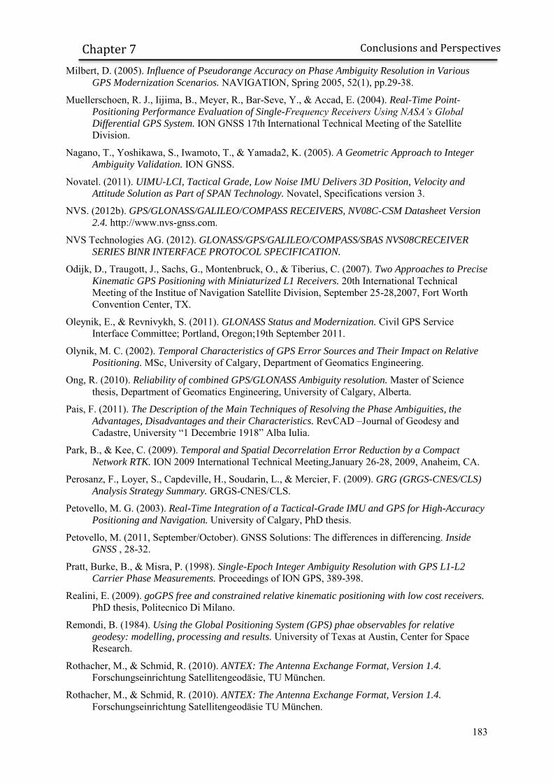
183
Conclusions and Perspectives
Chapter 7
Milbert, D. (2005). Influence of Pseudorange Accuracy on Phase Ambiguity Resolution in Various
GPS Modernization Scenarios. NAVIGATION, Spring 2005, 52(1), pp.29-38.
Muellerschoen, R. J., Iijima, B., Meyer, R., Bar-Seve, Y., & Accad, E. (2004). Real-Time Point-
Positioning Performance Evaluation of Single-Frequency Receivers Using NASA’s Global
Differential GPS System. ION GNSS 17th International Technical Meeting of the Satellite Division.
Nagano, T., Yoshikawa, S., Iwamoto, T., & Yamada2, K. (2005). A Geometric Approach to Integer
Ambiguity Validation. ION GNSS.
Novatel. (2011). UIMU-LCI, Tactical Grade, Low Noise IMU Delivers 3D Position, Velocity and
Attitude Solution as Part of SPAN Technology. Novatel, Specifications version 3.
NVS. (2012b). GPS/GLONASS/GALILEO/COMPASS RECEIVERS, NV08C-CSM Datasheet Version
2.4. http://www.nvs-gnss.com.
NVS Technologies AG. (2012). GLONASS/GPS/GALILEO/COMPASS/SBAS NVS08CRECEIVER
SERIES BINR INTERFACE PROTOCOL SPECIFICATION.
Odijk, D., Traugott, J., Sachs, G., Montenbruck, O., & Tiberius, C. (2007). Two Approaches to Precise
Kinematic GPS Positioning with Miniaturized L1 Receivers. 20th International Technical Meeting of the Institue of Navigation Satellite Division, September 25-28,2007, Fort Worth Convention Center, TX.
Oleynik, E., & Revnivykh, S. (2011). GLONASS Status and Modernization. Civil GPS Service Interface Committee; Portland, Oregon;19th September 2011.
Olynik, M. C. (2002). Temporal Characteristics of GPS Error Sources and Their Impact on Relative
Positioning. MSc, University of Calgary, Department of Geomatics Engineering.
Ong, R. (2010). Reliability of combined GPS/GLONASS Ambiguity resolution. Master of Science thesis, Department of Geomatics Engineering, University of Calgary, Alberta.
Pais, F. (2011). The Description of the Main Techniques of Resolving the Phase Ambiguities, the
Advantages, Disadvantages and their Characteristics. RevCAD –Journal of Geodesy and Cadastre, University “1 Decembrie 1918” Alba Iulia.
Park, B., & Kee, C. (2009). Temporal and Spatial Decorrelation Error Reduction by a Compact
Network RTK. ION 2009 International Technical Meeting,January 26-28, 2009, Anaheim, CA.
Perosanz, F., Loyer, S., Capdeville, H., Soudarin, L., & Mercier, F. (2009). GRG (GRGS-CNES/CLS)
Analysis Strategy Summary. GRGS-CNES/CLS.
Petovello, M. G. (2003). Real-Time Integration of a Tactical-Grade IMU and GPS for High-Accuracy
Positioning and Navigation. University of Calgary, PhD thesis.
Petovello, M. (2011, September/October). GNSS Solutions: The differences in differencing. Inside
GNSS , 28-32.
Pratt, Burke, B., & Misra, P. (1998). Single-Epoch Integer Ambiguity Resolution with GPS L1-L2
Carrier Phase Measurements. Proceedings of ION GPS, 389-398.
Realini, E. (2009). goGPS free and constrained relative kinematic positioning with low cost receivers. PhD thesis, Politecnico Di Milano.
Remondi, B. (1984). Using the Global Positioning System (GPS) phae observables for relative
geodesy: modelling, processing and results. University of Texas at Austin, Center for Space Research.
Rothacher, M., & Schmid, R. (2010). ANTEX: The Antenna Exchange Format, Version 1.4. Forschungseinrichtung Satellitengeodäsie, TU München.
Rothacher, M., & Schmid, R. (2010). ANTEX: The Antenna Exchange Format, Version 1.4. Forschungseinrichtung Satellitengeodäsie TU München.

184
Conclusions and Perspectives
Chapter 7
Salos Andres, C. D. (2012). Integrity Monitoring applied to the reception of GNSS signals in urban
environements. PhD thesis, Institut National Polytechnique de Toulouse.
Sanz Subirana, J., Juan Zornoza, J., & Hernández-Pajares, M. (2011). Transformations between ECEF
and ENU coordinates. Navipedia, ESA,http://www.navipedia.net.
Schroth, G., Ene, A., Blanch, J., Walter, T., & Enge, P. (2008). Failure Detection and Exclusion via
Range Consensus. Proceedings of European Navigation Conference,2008.
Serrano, L., Kim, D., & Langley, R. (2005). A New Carrier-Phase Multipath Observable for GPS
RealTime Kinematics, Based on Between Receiver Dynamics. Proceedings of the 61st Annual Meeting of The Institute of Navigation, June 27 - 29, 2005,Cambridge, MA.
Shi, J., & Gao, Y. (2012). A Fast Integer Ambiguity Resolution Method for PPP. Proceedings of ION GNSS 2012, September 17-21, 2012, Nashville, Tenessee.
Shin, E.-H. (2001). Accuracy Improvement of Low-Cost INS/GPS for Land Applications. Department of Geomatics Engineering, Calgary, Alberta.
Shirai, T., & Kubo, N. (2011). RTK-GPS Reliability Improvement in Dense Urban Areas. ION GNSS, Portland, OR.
Sleewaegen, J., & Boon, F. (2001). Mitigating Short-Delay Multipath: a Promising New Technique. 14th International Technical Meeting of the Satellite Division of the Institute of Navigation,September 11-14, 2001.
Sleewaegen, J., Simsky, A., de Wilde, W., Boon, F., & Willems, T. (2012, May/June). Demystifying GLONASS Inter-Frequency Carrier Phase Biases. Inside GNSS , 57-61.
Steingass, A., & Lehner, A. (2008). Differences in Multipath Propagation Between Urban and
Suburban Environments. ION GNSS 21st. International Technical Meeting of the Satellite Division, 16-19, September 2008, Savannah, GA.
Suh, Y., Konishi, Y., Hakamata, T., & Shibasaki, R. (2003). Evaluation of Positioning Service Level
for Intelligent Transportation Systems in Urban Area using a Simulation Tool . ION GPS/GNSS 2003,9-12 September 2003, Portland, OR.
Sukkarieh, S. (2000). Low Cost, High Integrity, Aided Inertial Navigation Systems for Autonomous
Land Vehicle. PhD thesis, Department of Mechanical and Mechatronic Engineering, The University of Sydney.
Takac, F. (2009). GLONASS inter-frequency biases and ambiguity resolution. Inside GNSS,vol. 2, no. 4, March/April 2009, pp. 24-28.
Takac, F., & Alves, P. (2012). GLONASS RTK Interoperability Issues Involving 3rd Party Receivers. Presentations of IGS Bias Workshop, January 2012, University of Bern, Switzerland.
Takasu. (2011). GNSS Precise Positioning with RTKLIB Part 2. IPNT-J Seminar, Tokyo, April 26, 2011.
Takasu, T. (2009). RTKLib: Open Source Program Package for RTK-GPS. Tokyo: FOSS4G.
Takasu, T., & Yasuda, A. (2008). Cycle Slip Detection and Fixing by MEMS-IMU/GPS Integration for
Mobile Environment RTK-GPS. ION GNSS 21st International Technical Meeting of the Satellite Division, 16-19, September 2008, Savannah, GA.
Takasu, T., & Yasuda, A. (2009). Development of the low-cost RTK-GPS receiver with an open source
program package RTKLIB. International Symposium on GPS/GNSS, International Convention Center Jeju, Korea, November 4-6, 2009 (rev.A submitted).
Takasu, T., & Yasuda, A. (2008b). Evaluation of RTK-GPS Performance with Low-cost Single-
frequency GPS Receivers. International Symposium on GPS/GNSS 2008, November 11-14, 2008, Tokyo International Exchange Center, Japan.
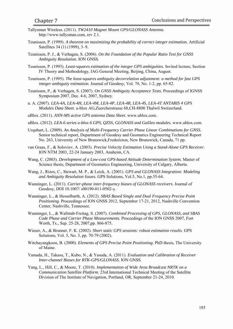
185
Conclusions and Perspectives
Chapter 7
Tallysman Wireless. (2011). TW2410 Magnet Mount GPS/GLONASS Antenna. http://www.tallysman.com, rev 2.1.
Teunissen, P. (1999). A theorem on maximizing the probability of correct integer estimation. Artificial Satellites 34 (1) (1999), 3–9.
Teunissen, P. J., & Verhagen, S. (2004). On the Foundation of the Popular Ratio Test for GNSS
Ambiguity Resolution. ION GNSS.
Teunissen, P. (1993). Least-squares estimation of the integer GPS ambiguities. Invited lecture, Section IV Theory and Methodology, IAG General Meeting, Beijing, China, August.
Teunissen, P. (1995). The least-squares ambiguity decorrelation adjustment: a method for fast GPS
integer ambiguity estimation. Journal of Geodesy, Vol. 70, No. 1-2, pp. 65-82.
Teunissen, P., & Verhagen, S. (2007). On GNSS Ambiguity Acceptance Tests. Proceedings of IGNSS Symposium 2007, Dec. 4-6, 2007, Sydney.
u. A. (2007). LEA-4A, LEA-4H, LEA-4M, LEA-4P, LEA-4R, LEA-4S, LEA-4T ANTARIS 4 GPS
Modules Data Sheet. u-blox AG,Zuercherstrasse 68,CH-8800 Thalwil Switzerland.
uBlox. (2011). ANN-MS active GPS antenna Data Sheet. www.ublox.com.
uBlox. (2012). LEA-6 series u-blox 6 GPS, QZSS, GLONASS and Galileo modules. www.ublox.com.
Urquhart, L. (2009). An Analysis of Multi-Frequency Carrier Phase Linear Combinations for GNSS. Senior technical report, Department of Geodesy and Geomatics Engineering Technical Report No. 263, University of New Brunswick,Fredericton, New Brunswick, Canada, 71 pp.
van Graas, F., & Soloviev, A. (2003). Precise Velocity Estimation Using a Stand-Alone GPS Receiver. ION NTM 2003, 22-24 January 2003, Anaheim, CA.
Wang, C. (2003). Development of a Low-cost GPS-based Attitude Determination System. Master of Science thesis, Department of Geomatics Engineering, University of Calgary, Alberta.
Wang, J., Rizos, C., Stewart, M. P., & Leick, A. (2001). GPS and GLONASS Integration: Modeling
and Ambiguity Resolution Issues. GPS Solutions, Vol.5, No.1, pp.55-64.
Wanninger, L. (2011). Carrier-phase inter-frequency biases of GLONASS receivers. Journal of Geodesy, DOI 10.1007/ s00190-011-0502-y.
Wanninger, L., & Hesselbarth, A. (2012). SBAS Based Single and Dual Frequency Precise Point
Positioning. Proceedings of ION GNSS 2012, September 17-21, 2012, Nashville Convention Center, Nashville, Tennessee.
Wanninger, L., & Wallstab-Freitag, S. (2007). Combined Processing of GPS, GLONASS, and SBAS
Code Phase and Carrier Phase Measurements. Proceedings of the ION GNSS 2007, Fort Worth, Tx., Sep. 25-28, 2007,pp. 866-875.
Wieser, A., & Brunner, F. K. (2002). Short static GPS sessions: robust estimation results. GPS Solutions, Vol. 5, No. 3, pp. 70-79 (2002).
Witchayangkoon, B. (2000). Elements of GPS Precise Point Positioning. PhD thesis, The University of Maine.
Yamada, H., Takasu, T., Kubo, N., & Yasuda, A. (2011). Evaluation and Calibration of Receiver
Inter-channel Biases for RTK-GPS/GLONASS. ION GNSS.
Yang, L., Hill, C., & Moore, T. (2010). Implementation of Wide Area Broadcast NRTK on a
Communication Satellite Platform. 23rd International Technical Meeting of the Satellite Division of The Institute of Navigation, Portland, OR, September 21-24, 2010.

186
APPENDIX
APPENDIX A.: Satellite clock and orbit correction model In order to remove the satellite clock bias and satellite hardware bias, corrections are applied to the
measurements by the user. These available corrections are related to one specific combination of
observations and corrects for both the satellite clock and the satellite hardware bias for this
combination. For example, the satellite clock correction transmitted within the navigation message
includes the satellite clock and the satellite hardware bias corresponding to the ionosphere-free
code combination. This correction can be expressed as
. As a consequence, when applying
directly the satellite clock correction included in the navigation message:
(A.1)
If a single-frequency user applies the broadcasted satellite clock directly, a satellite bias
will remain:
(A.2)
In order to obtain an unbiased position, a correction called “Time Group Delay (TGD)” broadcasted in
the navigation message has to be applied (
):
(A.3)
It can be deduced that

187
APPENDIX
Integer PPP satellite clock correction from GRG or PPP-Wizard project corrects for both the satellite
clock delay and the satellite hardware bias for the ionosphere-free phase combination. It is thus
equivalent to
. This means that:
(A.4)
Finally, satellite orbit corrections are estimated together with satellite clock corrections. Therefore, it
is expected that satellite clock corrections are heavily correlated with orbit radial error. Then, it is
important to use orbits and satellite clock from a same source of corrections (broadcasted message,
IGS product or integer PPP products) and not to mix corrections coming from different sources.

188
APPENDIX
APPENDIX B.: Linking Time-differenced Geometric Range to Time-differenced Position
Following [van Graas, et al., 2003], the time-differenced geometric range can be expressed as such:
( ) ( )
( ) [ ( ) ( )] ( ) [ ( ) ( )]
Where:
( ) is the user to satellite line-of-sight vector at time
( ) is the satellite position vector in the ECEF reference frame at time
( ) is the user position vector at time
Notations are summarized on Figure B.1.
Figure B.1 Time-differenced model geometry
Expressing as a function of ( ) ( ):
( ) [ ( ) ( )] ( ) [ ( ) ( )]
( ) ( ) ( ) ( ) ( ) ( ) ( ) ( )

189
APPENDIX
( ) ( ) ( ) ( )⏟
[ ( ) ( )] ( )⏟
( )
Satellite average Doppler and relative LOS change corrections are very sensitive to user position and
satellite position error. Moreover, discussions on the impact of atmospheric delay, satellite clock bias
and relativistic effect on time-differenced model can be found in [van Graas, et al., 2003]. In this
paper, tropospheric delay was corrected using UNB3m model [Leandro, et al., 2006] and satellite
clock was corrected using broadcast ephemeris. If broadcast ephemeris are used, special attention must
be paid to epochs when ephemeris are updated. The same ephemeris has to be used for time and .

190
APPENDIX
APPENDIX C.: RTKLIB Configuration Description The RTKLIB configuration used in 5.1.6.2 and 5.2.6.3 is illustred on Figure C.1 to C.4.
Figure C.1 RTKLIB Setting 1 tab
Figure C.2 RTKLIB Setting 2 tab
Figure C.3 RTKLIB Statistics tab
Figure C.4 RTKLIB Misc tab

191
APPENDIX
APPENDIX D.: Impact of the Virtual Null Velocity Observation in the Vertical Direction on the Performance of the RTK Filter
In this paragraph, the RTK filter is tested without the null velocity observation in the vertical direction.
The RTK filter is tested in its reference configuration, as described in 6.1.1. Results can be found on
Figure D.1 to D.4 for the 2 data sets.
Figure D.1 Difference between estimated trajectory and
reference trajectory in downtown Toulouse (data set 1). Black
asterisk represents epochs when ambiguity vector is validated and
fixed as integer
Figure D.2 Difference between estimated trajectory and
reference trajectory on Toulouse’s beltway (data set 1). Black
asterisk represents epochs when ambiguity vector is validated and
fixed as integer
09:15 09:20 09:25 09:30 09:35 09:40-10
-8
-6
-4
-2
0
2
4
6
8
10Error in the estimated position (Downtown Toulouse)
Time of Day (hours:minutes)
mete
rs
Up
East
North
Fix mode
09:45 09:50 09:55-10
-8
-6
-4
-2
0
2
4
6
8
10Error in the estimated position (Toulouse's beltway)
Time of Day (hours:minutes)
mete
rs
Up
East
North
Fix mode

192
APPENDIX
Figure D.3 Difference between estimated trajectory and
reference trajectory in downtown Toulouse (data set 2). Black
asterisk represents epochs when ambiguity vector is validated and
fixed as integer
Figure D.4 Difference between estimated trajectory and
reference trajectory on Toulouse’s beltway (data set 2). Black
asterisk represents epochs when ambiguity vector is validated and
fixed as integer
Compared to results obtained in 6.1, the vertical component is greatly smoothed, notably in urban
environment. Indeed, the variance associated to the null velocity depends on the speed of the vehicle,
as explained in 4.2.1.1. The slower the vehicle is, the larger the impact of the virtual observation on
the estimated position.
The gain in the horizontal domain is however modest compared to the results obtained in Table 6.1, as
seen on Table D.1. Table D.1 Summary of the performance of the RTK filter without the vertical velocity constraint, using the
reference configuration
horizontal position error
68th percentile 95th percentile 99th percentile Fix rate Wrong Fix rate
Data Set 1 2.60 meters 5.82 meters 7.24 meters 0% 0%
urban 2.78 meters 6.54 meters 7.25 meters 0% 0%
Beltway 2.07 meters 3.46 meters 4.31 meters 0% 0%
Data Set 2 2.21 meters 5.81 meters 10.83 meters 0% 0%
urban 3.05 meters 6.89 meters 12.27 meters 0% 0%
beltway 1.33 meters 2.13 meters 2.47 meters 0% 0%
12:30 12:45 13:00 13:15 13:30-10
-8
-6
-4
-2
0
2
4
6
8
10Error in the estimated position (Downtown Toulouse)
Time of Day (hours:minutes)
mete
rs
Up
East
North
Fix mode
13:40 13:50 14:00 14:10 14:20-10
-8
-6
-4
-2
0
2
4
6
8
10Error in the estimated position (Toulouse's beltway)
Time of Day (hours:minutes)
mete
rs
Up
East
North
Fix mode

193
APPENDIX
APPENDIX E.: Instantaneous Single-Frequency PPP Initialization In this paragraph, the instantaneous initialization of the single-frequency PPP algorithm is tested. As
this algorithm is intended to cope with loss of the communication link in a relatively friendly
environment, a communication link outage will be simulated at the beginning of the first data set. The
receiver was static but the Kalman filter was tuned with the acceleration process noise described in
6.1.1. At the first epoch, the RTK ambiguities are used to initialize the single-frequency PPP filter
ambiguities, as explained in 4.3.3. The position obtained with the PPP filter is then compared to a
single-point positioning Kalman filter with similar tuning. In the PPP filter, position and ambiguities
are initialized using the technique described in 4.3.3. In the second case, the position is initialized
using the fixed position from the RTK software as well as its associated covariance.
The description of the different parameters and corrections used in both filters is presented in Table
E.1. Table E.1 Parameters of the GRAPHIC PPP Kalman filter and the Single-Point Kalman filter
GRAPHIC PPP filter Single-Point filter
Observations used GRAPHIC combination
Doppler measurements L1 code measurements Doppler measurements
Ionospheric correction
NO YES (Klobuchar model)
Kalman filter Acceleration process noise
Ephemeris used IGS final ephemeris IGS final ephemeris
Results can be found on Figure E.2 and Figure E.2. In both case, the filters are initialized just after
9:01. In the case of the Single-Point positioning filter, the position slowly drifts from the true position,
as pseudorange measurements are affected by unmodelled ionospheric delay and multipath error. The
drift is slow as Doppler measurements smooth the solution evolution in the position domain. In the
second case, the combination is ionosphere-free and 2 times less affected by multipath error on code
measurements. Therefore, estimated position remains very close from the true position and the
improvement is significant.

194
APPENDIX
Figure E.1 Position error obtained using the Single-Point
positioning algorithm initialized with the fixed RTK position.
Figure E.2 Position error obtained using the single-frequency
PPP filter algorithm with position and ambiguities initialized
using the proposed technique.
However, this level of accuracy is kept only if carrier phase measurements are continuously tracked. In
the case of an unrepaired cycle slip or a loss of lock, the precisely initialized ambiguities of the PPP
filter have to be estimated again, implying a lengthy convergence time.
09:01 09:02 09:03 09:04 09:05-4
-3
-2
-1
0
1
2
3
4Error using Single-Point positioning
Time of Day (hours:minutes)
mete
rs
Up
East
North
09:01 09:02 09:03 09:04 09:05-4
-3
-2
-1
0
1
2
3
4Error using Single-Point positioning
Time of Day (hours:minutes)
mete
rs
Up
East
North
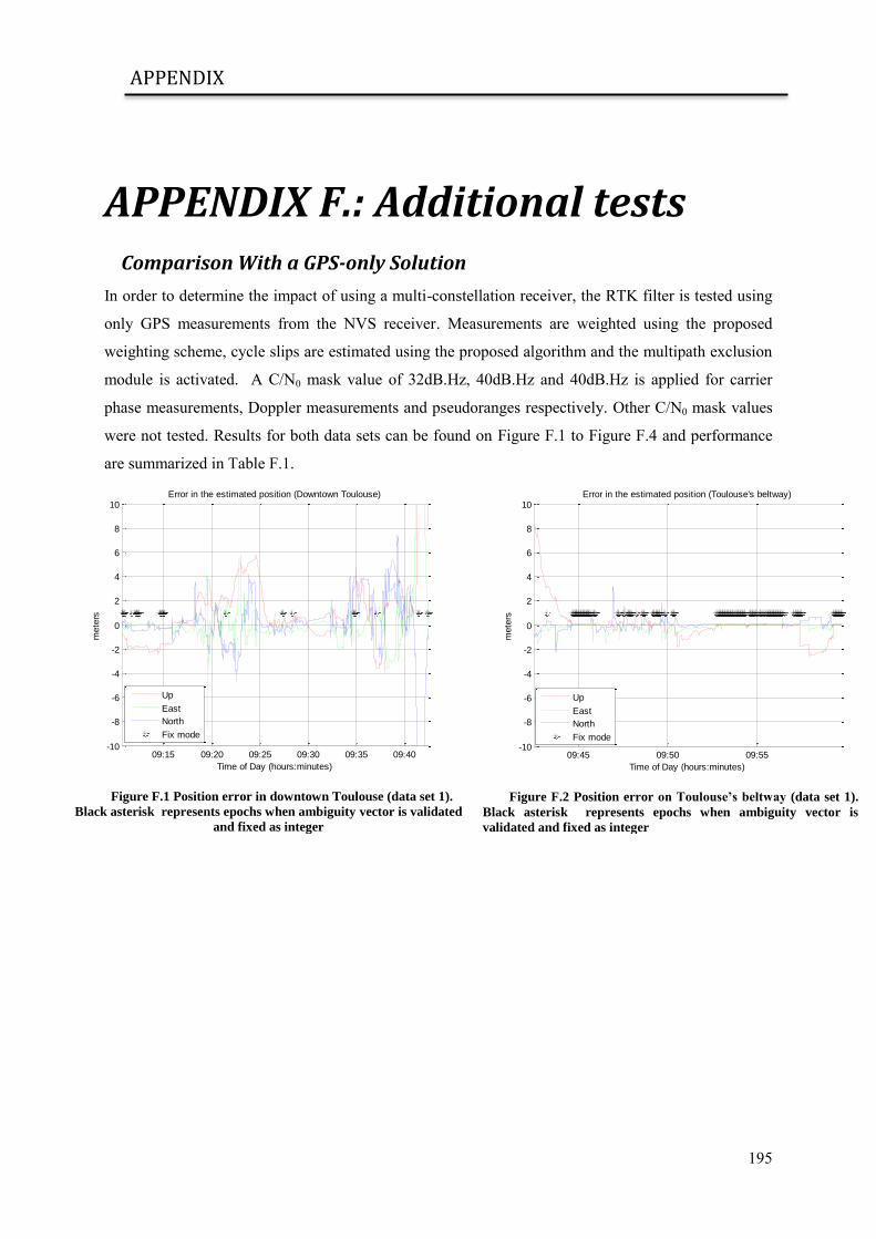
195
APPENDIX
APPENDIX F.: Additional tests Comparison With a GPS-only Solution
In order to determine the impact of using a multi-constellation receiver, the RTK filter is tested using
only GPS measurements from the NVS receiver. Measurements are weighted using the proposed
weighting scheme, cycle slips are estimated using the proposed algorithm and the multipath exclusion
module is activated. A C/N0 mask value of 32dB.Hz, 40dB.Hz and 40dB.Hz is applied for carrier
phase measurements, Doppler measurements and pseudoranges respectively. Other C/N0 mask values
were not tested. Results for both data sets can be found on Figure F.1 to Figure F.4 and performance
are summarized in Table F.1.
Figure F.1 Position error in downtown Toulouse (data set 1).
Black asterisk represents epochs when ambiguity vector is validated
and fixed as integer
Figure F.2 Position error on Toulouse’s beltway (data set 1).
Black asterisk represents epochs when ambiguity vector is
validated and fixed as integer
09:15 09:20 09:25 09:30 09:35 09:40-10
-8
-6
-4
-2
0
2
4
6
8
10Error in the estimated position (Downtown Toulouse)
Time of Day (hours:minutes)
mete
rs
Up
East
North
Fix mode
09:45 09:50 09:55-10
-8
-6
-4
-2
0
2
4
6
8
10Error in the estimated position (Toulouse's beltway)
Time of Day (hours:minutes)
mete
rs
Up
East
North
Fix mode
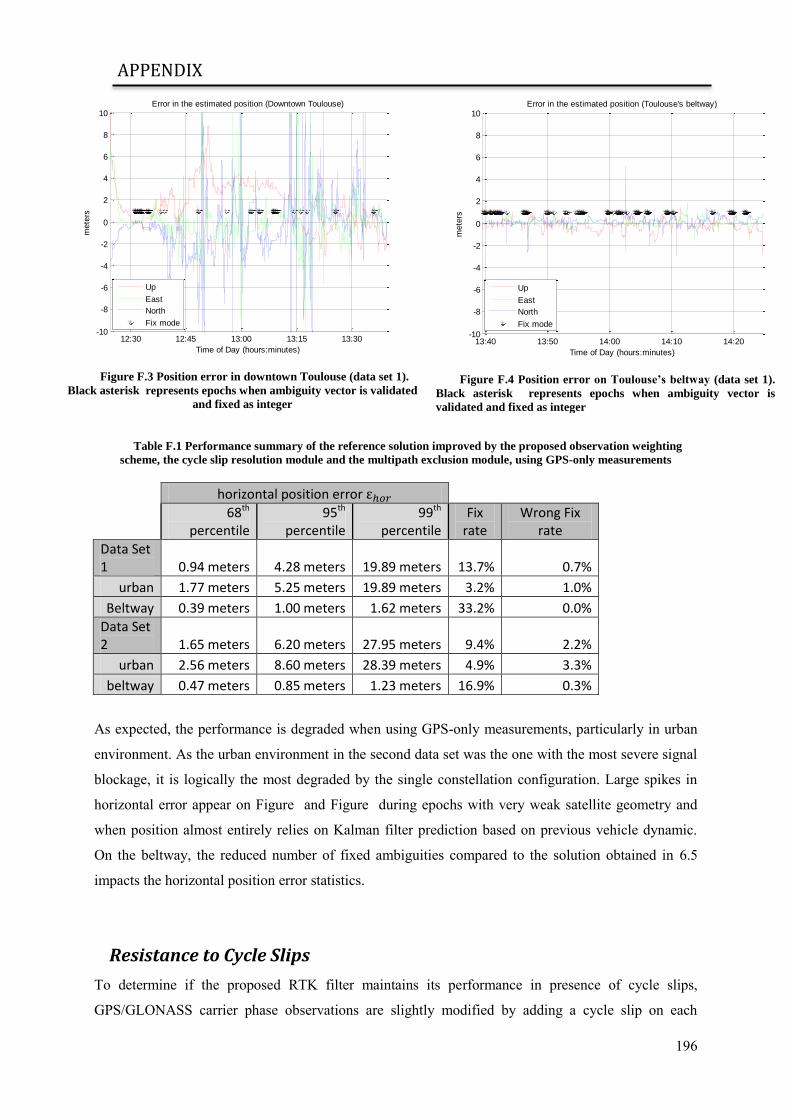
196
APPENDIX
Figure F.3 Position error in downtown Toulouse (data set 1).
Black asterisk represents epochs when ambiguity vector is validated
and fixed as integer
Figure F.4 Position error on Toulouse’s beltway (data set 1).
Black asterisk represents epochs when ambiguity vector is
validated and fixed as integer
Table F.1 Performance summary of the reference solution improved by the proposed observation weighting
scheme, the cycle slip resolution module and the multipath exclusion module, using GPS-only measurements
horizontal position error
68th percentile
95th percentile
99th percentile
Fix rate
Wrong Fix rate
Data Set 1 0.94 meters 4.28 meters 19.89 meters 13.7% 0.7%
urban 1.77 meters 5.25 meters 19.89 meters 3.2% 1.0%
Beltway 0.39 meters 1.00 meters 1.62 meters 33.2% 0.0%
Data Set 2 1.65 meters 6.20 meters 27.95 meters 9.4% 2.2%
urban 2.56 meters 8.60 meters 28.39 meters 4.9% 3.3%
beltway 0.47 meters 0.85 meters 1.23 meters 16.9% 0.3%
As expected, the performance is degraded when using GPS-only measurements, particularly in urban
environment. As the urban environment in the second data set was the one with the most severe signal
blockage, it is logically the most degraded by the single constellation configuration. Large spikes in
horizontal error appear on Figure and Figure during epochs with very weak satellite geometry and
when position almost entirely relies on Kalman filter prediction based on previous vehicle dynamic.
On the beltway, the reduced number of fixed ambiguities compared to the solution obtained in 6.5
impacts the horizontal position error statistics.
Resistance to Cycle Slips
To determine if the proposed RTK filter maintains its performance in presence of cycle slips,
GPS/GLONASS carrier phase observations are slightly modified by adding a cycle slip on each
12:30 12:45 13:00 13:15 13:30-10
-8
-6
-4
-2
0
2
4
6
8
10Error in the estimated position (Downtown Toulouse)
Time of Day (hours:minutes)
mete
rs
Up
East
North
Fix mode
13:40 13:50 14:00 14:10 14:20-10
-8
-6
-4
-2
0
2
4
6
8
10Error in the estimated position (Toulouse's beltway)
Time of Day (hours:minutes)
mete
rs
Up
East
North
Fix mode

197
APPENDIX
satellite at each epoch. Each cycle slip is a randomly chosen integer between -100 and 100. The 2 data
sets are then processed with the same configuration than in 6.5. Results can be found on Figure F.5 to
Figure F.8 and performance is summarized in Table F.2. It can be seen that performance is generally
only slightly degraded by the addition of cycle slips. The performance degradation occurs during
epochs when the hypothesis test “there is no cycle slip” using phase only measurements would have
been passed if no cycle slip was present, but the integer cycle slip resolution fails because of weak
satellite geometry or low accuracy of Doppler measurements. It can be seen that the horizontal
position error on the beltway in the first data set is slightly improved in presence of cycle slips. It is
due to the wrong fix that occurs just after 9:40 on Figure 6.29 which is not present when cycle slips
are added.
Figure F.5 Position error in downtown Toulouse (data set 1).
Black asterisk represents epochs when ambiguity vector is validated
and fixed as integer
Figure F.6 Position error on Toulouse’s beltway (data set 1).
Black asterisk represents epochs when ambiguity vector is
validated and fixed as integer
09:15 09:20 09:25 09:30 09:35 09:40-10
-8
-6
-4
-2
0
2
4
6
8
10Error in the estimated position (Downtown Toulouse)
Time of Day (hours:minutes)
mete
rs
Up
East
North
Fix mode
09:45 09:50 09:55-10
-8
-6
-4
-2
0
2
4
6
8
10Error in the estimated position (Toulouse's beltway)
Time of Day (hours:minutes)
mete
rs
Up
East
North
Fix mode

198
APPENDIX
Figure F.7 Position error in downtown Toulouse (data set 2).
Black asterisk represents epochs when ambiguity vector is validated
and fixed as integer
Figure F.8 Position error on Toulouse’s beltway (data set 2).
Black asterisk represents epochs when ambiguity vector is
validated and fixed as integer
Table F.2 Performance summary of the reference solution improved by GLONASS code inter-channel bias
correction, the proposed observation weighting scheme, the cycle slip resolution module, the multipath exclusion
module and the addition of GLONASS ambiguities when a cycle slip is added at each epoch on each satellite
Horizontal Position Error
68th percentile 95th percentile 99th percentile Fix rate Wrong Fix rate
Data Set 1 0.90 meters 2.95 meters 3.95 meters 32.3% 0.8%
urban 1.34 meters 3.47 meters 4.24 meters 16.0% 2.6%
Beltway 0.14 meters 0.89 meters 1.30 meters 62.6% 0.0%
Data Set 2 0.92 meters 3.30 meters 6.01 meters 21.2% 2.5%
urban 1.50 meters 3.99 meters 6.85 meters 7.9% 11.0%
beltway 0.23 meters 0.71 meters 0.97 meters 43.4% 0.0%
APPENDIX G.: Description of the implemented software
The proposed solution has been implemented from scratch, as a Matlab software. It includes all the
algorithms proposed in this PhD study, notably:
Cycle slip resolution module
Multipath detection module
12:30 12:45 13:00 13:15 13:30-10
-8
-6
-4
-2
0
2
4
6
8
10Error in the estimated position (Downtown Toulouse)
Time of Day (hours:minutes)
mete
rs
Up
East
North
Fix mode
13:40 13:50 14:00 14:10 14:20-10
-8
-6
-4
-2
0
2
4
6
8
10Error in the estimated position (Toulouse's beltway)
Time of Day (hours:minutes)
mete
rs
Up
East
North
Fix mode

199
APPENDIX
RTK (with GPS/GLONASS ambiguity resolution module ) and single-frequency PPP
Kalman filter
GLONASS code and carrier phase biases calibration module, in post-processing mode
Additionally, all functions required by the previous modules have been encoded:
Import of RINEX files (GPS/GLONASS/SBAS observations and navigation files)
Import of precise ephemeris files (.sp3 files), ANTEX files…
Import of EMS (EGNOS) files for ionospheric corrections
Computation of satellite position and satellite clock offset values for the different
constellations
Additionally a complete set of functions has been designed to analyze, plot and compare data statistics
and performance results.