symmetryS S

Article

Skein Invariants of Links and Their StateSum Models

Louis H. Kauffman 1,† and Sofia Lambropoulou 2,*,†

1 Department of Mathematics, Statistics and Computer Science, University of Illinois at Chicago, Chicago,IL 60607-7045, USA; kauffman@math.uic.edu

2 School of Applied Mathematical and Physical Sciences, National Technical University of Athens,15780 Athens, Greece

* Correspondence: sofia@math.ntua.gr; Tel.: +30-210-772-1346† These authors contributed equally to this work.

Received: 19 September 2017; Accepted: 9 October 2017; Published: 13 October 2017

Abstract: We present the new skein invariants of classical links, H[H], K[K] and D[D], basedon the invariants of links, H, K and D, denoting the regular isotopy version of the Homflyptpolynomial, the Kauffman polynomial and the Dubrovnik polynomial. The invariants are obtainedby abstracting the skein relation of the corresponding invariant and making a new skein algorithmcomprising two computational levels: first producing unlinked knotted components, then evaluatingthe resulting knots. The invariants in this paper, were revealed through the skein theoretic definitionof the invariants Θd related to the Yokonuma–Hecke algebras and their 3-variable generalizationΘ, which generalizes the Homflypt polynomial. H[H] is the regular isotopy counterpart of Θ.The invariants K[K] and D[D] are new generalizations of the Kauffman and the Dubrovnikpolynomials. We sketch skein theoretic proofs of the well-definedness and topological properties ofthese invariants. The invariants of this paper are reformulated into summations of the generatinginvariants (H, K, D) on sublinks of the given link L, obtained by partitioning L into collections ofsublinks. The first such reformulation was achieved by W.B.R. Lickorish for the invariant Θ and wegeneralize it to the Kauffman and Dubrovnik polynomial cases. State sum models are formulated forall the invariants. These state summation models are based on our skein template algorithm whichformalizes the skein theoretic process as an analogue of a statistical mechanics partition function.Relationships with statistical mechanics models are articulated. Finally, we discuss physical situationswhere a multi-leveled course of action is taken naturally.

Keywords: classical links; mixed crossings; skein relations; stacks of knots; Homflypt polynomial;Kauffman polynomial; Dubrovnik polynomial; 3-variable skein link invariant; closed combinatorialformula; state sums; double state summation; skein template algorithm

MSC: 57M27, 57M25

1. Introduction

In this paper, we present the new generalized skein invariants of links, H[H], D[D] and K[K],based on the regular isotopy version of the Homflypt polynomial, the Dubrovnik polynomial andthe Kauffman polynomial, respectively (Theorems 1–3). A link invariant is skein invariant if it can becomputed on each link solely by the use of skein relations and a set of initial conditions. The generalizedinvariants are evaluated via a two-level procedure: for a given link we first untangle its compoundknots using the skein relation of the corresponding basic invariant H, D or K and only then we evaluateon unions of unlinked knots by applying a new rule, which is based on the evaluation of H, D and

Symmetry 2017, 9, 226; doi:10.3390/sym9100226 www.mdpi.com/journal/symmetry

Symmetry 2017, 9, 226 2 of 29

K respectively. In particular, on knots (that is, one-component links) each one of the generalizedinvariants has the same evaluation as its underlying basic invariant.

We then show that each generalized invariant can be reformulated in terms of a closed formula,involving summation over evaluations of sublinks of the given link (Theorems 5–7). It is remarkablethat the generalized invariants have two such distinct faces, as skein invariants and as closedcombinatorial formuli. In this paper, we present both of these points of view and how they arerelated to state summations and possible relationships with statistical mechanics and applications.These constructions alter the philosophy of classical skein-theoretic techniques, whereby mixed as wellas self-crossings in a link diagram would get indiscriminately switched. Using a known skein invariant,one first unlinks all components using the skein relation and then one evaluates on unions of unlinkedknots using that skein invariant and at the same time introducing a new variable. This approach couldfind applications in physical systems where different constituents need to be separated first.

This paper is based on [1] where the reader can find more detailed treatment of much of the theory.There are not many known skein link invariants in the literature. Skein invariants include: the

Alexander–Conway polynomial [2,3], the Jones polynomial [4], and the Homflypt polynomial [5–8],which specializes to both the Alexander–Conway and the Jones polynomial; there is alsothe bracket polynomial [9], the Brandt–Lickorish–Millett–Ho polynomial [10], the Dubrovnikpolynomial and the Kauffman polynomial [11], which specializes to both the bracket and theBrandt–Lickorish–Millett–Ho polynomial. Finally, we have the Juyumaya–Lambropoulou familyof invariants ∆d,D, d ∈ N, for any non-empty subset D of Z/dZ [12], and the analogousChlouveraki–Juyumaya–Karvounis–Lambropoulou invariants Θd and their 3-variable generalizationΘ [13]. In fact, this last invariant Θ was our motivation for constructing the generalized invariants.The invariant H[H] is in fact the regular isotopy version of the invariant Θ and Theorem 1 can be usedto provide a self-contained skein theoretic proof of its existence.

The invariant Θ was discovered via the following path: In [12] a family of framed link invariantswas constructed via a Markov trace on the Yokonuma–Hecke algebras [14], which restrict to the familyof classical link invariants {∆d,D} [15]. These were studied in [15,16], especially their relation to theHomflypt polynomial, P, but topological comparison had not been possible due to algebraic anddiagrammatic difficulties. In [13,17,18] another presentation [19] was used for the Yokonuma–Heckealgebra and the related classical link invariants were now denoted Θd. The invariants Θd were thenrecovered via the skein relation of P that can only apply to mixed crossings of a link [13] and they wereshown to be distinct from P on links, for d 6= 1, but topologically equivalent to P on knots [13,17] (hencealso distinct from the Kauffman polynomial). Finally, the family of invariants {Θd}, which includesP for d = 1, was generalized to the new 3-variable skein link invariant Θ [13], which is also relatedto the theory of tied links [20]. A succinct exposition of the above results can be found in [21].These constructions opened the way to new research directions. Cf. [12,13,15–17,19,20,22–38].

Further, in [13] Appendix B, W.B.R. Lickorish provides a closed combinatorial formula for thedefinition of the invariant Θ, showing that it is a mixture of Homflypt polynomials and linkingnumbers of sublinks of a given link. The combinatorial formuli (7), (15) and (16) for the generalizedinvariants are inspired by the Lickorish formula. These closed formuli are remarkable summationsof evaluations on sublinks with certain coefficients, that surprisingly satisfy the analogous mixedskein relations, so they can be regarded by themselves as definitions of the invariants H[H], D[D] andK[K] respectively. Formula (7) shows that the strength of H[H] against H comes from its ability todistinguish certain sublinks of Homflypt-equivalent links. In [13] a list of six 3-component links aregiven, which are Homflypt equivalent but are distinguished by the invariant Θ and thus also by H[H].

We proceed with constructing state sum models associated to the generalized skein invariants.A state sum model is a sum over evaluations of combinatorial configurations (the states) related to thegiven link diagram, such that this sum is equal to the invariant that we wish to compute. The statesums are based on the skein template algorithm, as explained in [39,40], which formalizes the skeintheoretic process as an analogue of a statistical mechanics partition function and produces the states

Symmetry 2017, 9, 226 3 of 29

to be evaluated. Our state sums use the skein calculation process for the invariants, but have a newproperty in the present context. They have a double level due to the combination in our invariants ofa skein calculation combined with the evaluation of a specific invariant on the knots that are at thebottom of the skein process. If we choose a state sum evaluation of a different kind for this specificinvariant, then we obtain a double-level state sum of our new invariant.

The paper concludes with a discussion about possible relationships with reconnection in vorticesin fluids, strand switching and replication of DNA, particularly the possible relations with thereplication of Kinetoplast DNA, and we discuss the possibility of multiple levels in the quantumHall effect where one considers the braiding of quasi-particles that are themselves physical subsystemscomposed of multiple electron vortices centered about magnetic field lines.

The paper is organized as follows: In Section 2 we present the skein theoretic setting of the newskein 3-variable invariants that generalize the regular isotopy version of the Homflypt, the Dubrovnikand the Kauffman polynomials. In Section 3 we give the ambient isotopy reformulations of thegeneralized link invariants. In Section 4 we adapt the combinatorial formula of Lickorish to ourregular isotopy setting for the generalized skein invariants. In Section 5 we define associated state summodels for the new invariants, while in Section 6 the idea about double state summations is articulated.Finally, in Section 7 we discuss the context of statistical mechanics models and partition functions inrelation to multiple level state summations and in Section 8 we speculate about possible applicationsfor these ideas.

2. The Skein-Theoretic Setting for the Generalized Invariants

In this section, we define the general regular isotopy invariant for links, H[H], D[D] andK[K], which generalize the regular isotopy version of the Homflypt polynomial, H, the Dubrovnikpolynomial, D, and the Kauffman polynomial, K, respectively.

As usual, an oriented link is a link with an orientation specified for each component. In addition,a link diagram is a projection of a link on the plane with only finitely many double points, the crossings,which are endowed with information ‘under/over’. Two link diagrams are regularly isotopic if theydiffer by planar isotopy and by Reidemeister moves II and III (with all variations of orientations in thecase of oriented diagrams). A mixed crossing is a crossing between different components.

2.1. Defining H[H]

Let L denote the set of classical oriented link diagrams. Let L+ ∈ L be an oriented diagram witha positive crossing specified and let L− be the same diagram but with that crossing switched. Let alsoL0 indicate the same diagram but with the smoothing which is compatible with the orientations of theemanating arcs in place of the crossing. See (1). The diagrams L+, L−, L0 comprise a so-called orientedConway triple.

(1)

L+ L− L0

we then have the following:

Theorem 1 (cf. [1]). Let H(z, a) denote the regular isotopy version of the Homflypt polynomial. Then thereexists a unique regular isotopy invariant of classical oriented links H[H] : L → Z[z, a±1, E±1], where z, a andE are indeterminates, defined by the following rules:

1. On crossings involving different components the following mixed skein relation holds:

H[H](L+)− H[H](L−) = z H[H](L0),

where L+, L−, L0 is an oriented Conway triple,

Symmetry 2017, 9, 226 4 of 29

2. For a union of r unlinked knots, Kr := tri=1Ki, with r ≥ 1, it holds that:

H[H](Kr) = E1−r H(Kr).

We recall that the invariant H(z, a) is determined by the following rules:

(H1) For L+, L−, L0 an oriented Conway triple, the following skein relation holds:

H(L+)− H(L−) = z H(L0),

(H2) The indeterminate a is the positive curl value for H:

R( ) = a R( ) and R( ) = a−1 R( ),

(H3) On the standard unknot:R(©) = 1.

We also recall that the above defining rules imply the following:(H4) For a diagram of the unknot, U, H is evaluated by taking:

H(U) = awr(U),

where wr(U) denotes the writhe of U—instead of 1 that is the case in the ambientisotopy category.

(H5) H being the Homflypt polynomial, it is multiplicative on a union of unlinked knots,Kr := tr

i=1Ki. Namely, for η := a−a−1

z we have:

H(Kr) = ηr−1Πri=1H(Ki).

Consequently, the evaluation of H[H] on the standard unknot is H[H](©) = H(©) = 1.

Assuming Theorem 1 one can compute H[H] on any given oriented link diagram L ∈ L byapplying the following procedure: the skein rule (1) of Theorem 1 can be used to give an evaluation ofH[H](L+) in terms of H[H](L−) and H[H](L0) or of H[H](L−) in terms of H[H](L+) and H[H](L0).We switch mixed crossings so that the switched diagram is more unlinked than before. Applying thisprinciple recursively we obtain a sum with polynomial coefficients and evaluations of H[H] on unionsof unlinked knots. These are formed by the mergings of components caused by the smoothings in theskein relation (1). To evaluate H[H] on a given union of unlinked knots we then use the invariant Haccording to rule (2) of Theorem 1. Note that the appearance of the indeterminate E in rule (2) is thecritical difference between H[H] and H. Finally, evaluations on individual knotted components aredone with the use of H via formula (H5) above.

One could specialize the z, the a and the E in Theorem 1 in any way one wishes. For example,if a = 1 then H specializes to the Alexander–Conway polynomial [2,3]. If z =

√a− 1/

√a then H

becomes the unnormalized Jones polynomial [4]. In each case H[H] can be regarded as a generalizationof that polynomial.

The invariant H[H] generalizes H to a new 3-variable invariant for links. Indeed, H[H] coincideswith the regular isotopy version of the new 3-variable link invariant Θ of [13]. On the other hand,by normalizing H[H] to obtain its ambient isotopy counterpart, we have by Theorem 1 an independent,skein-theoretic proof of the well-definedness of Θ.

2.2. Defining D[D] and K[K]

We now consider the class Lu of unoriented link diagrams. For any crossing of a diagram of a linkin Lu, if we rotate the overcrossing arc counterclockwise it sweeps two regions out of the four. If we

Symmetry 2017, 9, 226 5 of 29

join these two regions, this is the A-smoothing of the crossing, while joining the other two regionsgives rise to the B-smoothing. Using these conventions, the A-smoothing of L+ in (2) below is L0 andthe B-smoothing of L+ is L∞. Similarly, the A-smoothing of L− is L∞ and the B-smoothing of L− isL0. We shall say that a crossing is of positive type if it produces a horizontal A-smoothing and that itis of negative type if it produces a vertical A-smoothing. Let now L+ be an unoriented diagram witha positive type crossing specified and let L− be the same diagram but with that crossing switched.Let also L0 and L∞ indicate the same diagram but with the A-smoothing and the B-smoothing in placeof the crossing. See (2). The diagrams L+, L−, L0, L∞ comprise a so-called unoriented Conway quadruple.

(2)

L+ L− L0 L∞

In analogy to Theorem 1 we also have the 3-variable generalizations of the regular isotopy versionsof the Dubrovnik and the Kauffman polynomials [11]:

Theorem 2 (cf. [1]). Let D(z, a) denote the regular isotopy version of the Dubrovnik polynomial. Then thereexists a unique regular isotopy invariant of classical unoriented links D[D] : Lu → Z[z, a±1, E±1], where z, aand E are indeterminates, defined by the following rules:

1. On crossings involving different components the following skein relation holds:

D[D](L+)− D[D](L−) = z(

D[D](L0)− D[D](L∞)),

where L+, L−, L0, L∞ is an unoriented Conway quadruple,2. For a union of r unlinked knots in Lu, Kr := tr

i=1Ki, with r ≥ 1, it holds that:

D[D](Kr) = E1−r D(Kr).

We recall that the invariant D(z, a) is determined by the following rules:

(D1) For L+, L−, L0, L∞ an unoriented Conway quadruple, the following skein relation holds:

D(L+)− D(L−) = z(

D(L0)− D(L∞)),

(D2) The indeterminate a is the positive type curl value for D:

D( ) = a D( ) and D( ) = a−1 D( ),

(D3) On the standard unknot:D(©) = 1.

We also recall that the above defining rules imply the following:(D4) For a diagram of the unknot, U, D is evaluated by taking

D(U) = awr(U),

(D5) D, being the Dubrovnik polynomial, it is multiplicative on a union of unlinked knots,Kr := tr

i=1Ki. Namely, for δ := a−a−1

z + 1 we have:

D(Kr) = δr−1Πri=1D(Ki).

Consequently, on the standard unknot we evaluate D[D](©) = D(©) = 1.

Symmetry 2017, 9, 226 6 of 29

The Dubrovnik polynomial, D, is related to the Kauffman polynomial, K, via the followingtranslation formula, observed by W.B.R Lickorish [11]:

D(L)(a, z) = (−1)c(L)+1 i−wr(L)K(L)(ia,−iz). (3)

Here, c(L) denotes the number of components of the link L ∈ Lu, i2 = −1, and wr(L) is thewrithe of L for some choice of orientation of L, which is defined as the algebraic sum of all crossingsof L. The translation formula is independent of the particular choice of orientation for L. Our theorygeneralizes also the regular isotopy version of the Kauffman polynomial [11] through the following:

Theorem 3 (cf. [1]). Let K(z, a) denote the regular isotopy version of the Kauffman polynomial. Then thereexists a unique regular isotopy invariant of classical unoriented links K[K] : Lu → Z[z, a±1, E±1], wherez, a and E are indeterminates, defined by the following rules:

1. On crossings involving different components the following skein relation holds:

K[K](L+) + K[K](L−) = z(K[K](L0) + K[K](L∞)

),

where L+, L−, L0, L∞ is an unoriented Conway quadruple,2. For a union of r unlinked knots in Lu, Kr := tr

i=1Ki, with r ≥ 1, it holds that:

K[K](Kr) = E1−r K(Kr).

We recall that the invariant K(z, a) is determined by the following rules:

(K1) For L+, L−, L0, L∞ an unoriented Conway quadruple, the following skein relation holds:

K(L+) + K(L−) = z(K(L0) + K(L∞)

),

(K2) The indeterminate a is the positive type curl value for K:

K( ) = a K( ) and K( ) = a−1 K( ),

(K3) On the standard unknot:K(©) = 1.

We also recall that the above defining rules imply the following:(K4) For a diagram of the unknot, U, K is evaluated by taking

K(U) = awr(U),

(K5) K, being the Kauffman polynomial, it is multiplicative on a union of unlinked knots,Kr := tr

i=1Ki. Namely, for γ := a+a−1

z − 1 we have:

K(Kr) = γr−1Πri=1K(Ki).

Consequently, on the standard unknot we evaluate K[K](©) = K(©) = 1.

In Theorems 2 and 3 the basic invariants D(z, a) and K(z, a) could be replaced by specializationsof the Dubrovnik and the Kauffman polynomial respectively and, then, the invariants D[D] and K[K]can be regarded as generalizations of these specialized polynomials. For example, if a = 1 then K(z, 1)is the Brandt–Lickorish–Millett–Ho polynomial [10] and if z = A + A−1 and a = −A3 then K becomesthe Kauffman bracket polynomial [9]. In both cases the invariant K[K] generalizes these polynomials.Furthermore, a formula analogous to (3) relates the generalized invariants D[D] and K[K], see (17).

Symmetry 2017, 9, 226 7 of 29

In order to prove Theorems 1–3 one needs to show that the computation of the correspondinggeneralized invariant can be done solely from the rules of the theorem and that it is independent fromany choices involved during the unlinking of different components as well as from the regular isotopymoves. To do this, we specify a computing algorithm to be used; but first we set some terminology.

2.3. Terminology and Notations

A link diagram is called generic if it is ordered, that is, an order c1, . . . , cr is given to its components,directed, that is, a direction is specified on each component, and based, that is, a basepoint is specifiedon each component, distinct from the double points of the crossings.

A diagram that is the union of r unlinked knots, Kr := tri=1Ki, with r ≥ 1, is said to be a

descending stack if, when walking along the components of Kr in their given order, starting from theirbasepoints and following the specified directions, every mixed crossing is first traversed along itsover-arc. Clearly, the structure of a descending stack no longer depends on the choice of basepoints;it is entirely determined by the order of its components. Note also that a descending stack is regularlyisotopic to the corresponding split link comprising the r knotted components, Ki, where the order ofcomponents is no longer relevant. The descending stack of knots associated to a given link diagram Lis denoted as dL.

2.4. Computing Algorithm for the Generalized Invariants

The generalized invariants are computed on two levels: on the first level one abstracts thecorresponding skein relation and applies it only on mixed crossings of a given link diagram. On thesecond level one evaluates the generalized invariant on unions of unlinked knots, by applying a new rulethat uses the corresponding ground invariant and introduces a new variable. More precisely, assumingTheorems 1–3 a generalized invariant can be easily computed on any link diagram L by applying thealgorithm below. This algorithm is necessary for proving well-definedness of the invariants.

1. (Diagrammatic level) Make L generic by choosing an order for its components and a basepoint and adirection on each component. Start from the basepoint of the first component and go along it in thechosen direction. When arriving at a mixed crossing for the first time along an under-arc we switchit by the mixed skein relation, so that we pass by the mixed crossing along the over-arc. At thesame time we smooth the mixed crossing, obtaining a new diagram in which the two componentsof the crossing merge into one. We repeat for all mixed crossings of the first component. Amongall resulting diagrams there is only one with the same number of crossings and the same numberof components as the initial diagram and in this one the first component gets unlinked fromthe rest and lies above all of them. The other resulting diagrams have one less crossing andhave the first component fused together with some other component. We proceed similarly withthe second component switching all its mixed crossings except for crossings involving the firstcomponent. In the end the second component gets unliked from all the rest and lies below thefirst one and above all others in the maximal crossing diagram, while we also obtain diagramscontaining mergings of the second component with others (except component one). We continuein the same manner with all components in order and we also apply this procedure to all productdiagrams coming from smoothings of mixed crossings. In the end we obtain the unlinked versionof L plus a number of links ` with unlinked components resulting from the mergings of differentcomponents.

2. (Computational level) On the level of the generalized invariant, Rule (1) of Theorems 1–3 tells ushow the switching of mixed crossings is controlled. After all applications of the mixed skeinrelation we obtain a linear sum of the values of the generalized invariant on all the resulting links` with unlinked components. The evaluation of the generalized invariant on each ` reduces to theevaluation of the corresponding basic invariant by Rule (2) of Theorems 1–3.

Symmetry 2017, 9, 226 8 of 29

2.5. Sketching the Proof of Theorems 1–3

For proving Theorems 1–3 one must prove that the resulting evaluation for a link diagram L doesnot depend on the choices made for bringing L to generic form, namely the sequence of mixed crossingchanges, the ordering of components and the choice of basepoints, and also that it is invariant underregular isotopy moves. A good guide for this is the skein-theoretic proof of Lickorish–Millett of thewell-definedness of the Homflypt polynomial [6], with the necessary adaptations and modifications,taking for granted the well-definedness of the basic invariant. The difference here lies in modifyingthe original skein method. The original method bottoms out on unlinks, since self-crossings are notdistinguished from mixed crossings. In the new method the evaluations bottom out on calculationsof the basic invariant on unions of unlinked knots. This difference causes the need of particularlyelaborate arguments in proving invariance of the resulting evaluation under the sequence of mixedcrossing switches and the order of components in comparison with [6].

Namely, we assume that the statement is valid for all link diagrams of up to n − 1 crossings,independently of choices made during the evaluation process and of Reidemeister III moves andReidemeister II moves that do not increase the number of crossings above n− 1. Our aim is to provethat the statement is valid for all generic link diagrams of up to n crossings, independently of choices,Reidemeister III moves and Reidemeister II moves not increasing above n crossings. We do this bydouble induction on the total number of crossings of a generic link diagram (which applied to allintermediate diagrams related to smoothings) and on the number of mixed crossing switches neededfor bringing the diagram to the form of a descending stack of knots (for which we make the assumptionthat rule (2) of the corresponding theorem applies).

The interested reader may consult [1] for a detailed exposition.

3. Translations to Ambient Isotopy

In this section, we provide the formuli for the corresponding ambient isotopy invariants,counterparts of the regular isotopy generalized invariants H[H], D[D] and K[K].

3.1. Normalization of H[H]

Let P denote the classical Homflypt polynomial. Then, as we know, one can obtain the ambientisotopy invariant P from its regular isotopy counterpart H via the formula:

P(L) := a−wr(L)H(L),

where wr(L) is the total writhe of the oriented diagram L. From our generalized regular isotopyinvariant H[H] one can derive an ambient isotopy invariant P[P] via:

P[P](L) := a−wr(L)H[H](L). (4)

Then for the invariant P[P] we have the following:

Theorem 4 (cf. [1]). Let P(z, a) denote the Homflypt polynomial. Then there exists a unique ambient isotopyinvariant of classical oriented links P[P] : L → Z[z, a±1, E±1] defined by the following rules:

1. On crossings involving different components the following skein relation holds:

a P[P](L+)− a−1 P[P](L−) = z P[P](L0),

where L+, L−, L0 is an oriented Conway triple.2. For Kr := tr

i=1Ki, a union of r unlinked knots, with r ≥ 1, it holds that:

P[P](Kr) = E1−r P(Kr).

Symmetry 2017, 9, 226 9 of 29

Remark 1. As pointed out in the Introduction, in Theorem 1 we could specialize the z, the a and the E inany way we wish. For example, if a = 1 then H(z, 1) becomes the Alexander–Conway polynomial, while ifz =√

a− 1/√

a then H(√

a− 1/√

a, a) becomes the unnormalized Jones polynomial. In each case H[H] canbe regarded as a generalization of that polynomial. Furthermore, the ambient isotopy invariant P[P] coincideswith the new 3-variable link invariant Θ(q, λ, E) [13], while for E = 1/d, P[P] coincides with the invariantΘd [12] (for E = 1 it coincides with P). So, our invariant P[P] is stronger than P and it coincides with theinvariant Θ. Hence, our proof of the existence of H[H] provides a direct skein-theoretic proof of the existenceof the invariant Θ, without the need of algebraic tools or the theory of tied links. Finally, for z =

√a− 1/

√a

the invariant P[P] can be renamed to V[V], V denoting the ambient isotopy version of the Jones polynomial,and it coincides with the new 2-variable link invariant θ(a, E) [33], which generalizes V and is stronger than V.We note that in [13,33] variables q and λ are used instead of z and a, coming from the algebraic background ofthe invariants, and in that context a = q−2 for the invariant θ.

3.2. Normalization of D[D] and K[K]

Let Y denote the classical ambient isotopy Dubrovnik polynomial. Then, one can obtain theambient isotopy invariant Y from its regular isotopy counterpart D via the formula:

Y(L) := a−wr(L)D(L),

where wr(L) is the total writhe of the diagram L for some choice of orientation of L. Analogously,and letting Z denote Y but with different variable, from our generalized regular isotopy invariantD[D] one can derive an ambient isotopy invariant Y[Y] via:

Y[Y](L) := a−wr(L)D[D](L). (5)

In order to have a skein relation one leaves it in regular isotopy form.As for the Dubrovnik polynomial, one can also define for the Kauffman polynomial the ambient

isotopy generalized invariant, counterpart of the regular isotopy generalized invariant K[K] constructedabove. Let K denote the classical regular isotopy Kauffman polynomial. Then, one can obtain theambient isotopy invariant F from its regular isotopy counterpart K via the formula:

F(L) := a−wr(L)K(L),

where wr(L) is the total writhe of the diagram L for some choice of orientation of L. Analogously,and letting S denote F but with different variable, from our generalized regular isotopy invariant K[K]one can derive an ambient isotopy invariant F[F] via:

F[F](L) := a−wr(L)K[K](L). (6)

In order to have a skein relation one leaves it in regular isotopy form.

4. Closed Combinatorial Formuli for the Generalized Invariants

4.1. A Closed Formula for H[H]

As we mentioned in the Introduction, in [13] Appendix B, W.B.R. Lickorish provides a closedcombinatorial formula for the definition of the invariant Θ = P[P], that uses the Homflypt polynomialsand linking numbers of sublinks of a given link. We will give here an analogous formula for ourregular isotopy extension H[H]. Namely:

Symmetry 2017, 9, 226 10 of 29

Theorem 5 (cf. [1]). Let L be an oriented link with n components. Then

H[H](L) =n

∑k=1

ηk−1Ek ∑π

H(πL) (7)

where the second summation is over all partitions π of the components of L into k (unordered) subsetsand H(πL) denotes the product of the Homflypt polynomials of the k sublinks of L defined by π.Furthermore, Ek = (E−1 − 1)(E−1 − 2) · · · (E−1 − k + 1) and η = a−a−1

z .

Proof. We present the proof in full detail, as we believe it is instructive and it proves the existence ofthe generalized invariants. Before proving the result, note the following equalities:

H(L1 t L2) = η H(L1) H(L2),

H[H](L1 t L2) =η

EH[H](L1) H[H](L2).

In the case where both L1 and L2 are knots the above formuli follow directly from rules (H5) and(2) above. If at least one of L1 and L2 is a true link, then the formuli follow by doing independent skeinprocesses on L1 and L2 for bringing them down to unlinked components, and then using the definingrules above.

Suppose now that a diagram of L is given. The proof is by induction on n and on the number, u,of crossing changes between distinct components required to change L to n unlinked knots. If n = 1there is nothing to prove. So assume the result true for n− 1 components and u− 1 crossing changesand prove it true for n and u.

The induction starts when u = 0. Then L is the union of n unlinked components L1, . . . , Ln. A classicelementary result concerning the Homflypt polynomial shows that H(L) = ηn−1H(L1) · · ·H(Ln).Furthermore, in this situation, for any k and π, H(πL) = ηn−kH(L1) · · ·H(Ln). Note thatH[H](L) = E1−nH(L) = ηn−1E1−nH(L1) · · ·H(Ln). So it is required to prove that

ηn−1E1−n = ηn−1n

∑k=1

S(n, k)(E−1 − 1)(E−1 − 2) · · · (E−1 − k + 1), (8)

where S(n, k) is the number of partitions of a set of n elements into k subsets. Now it remains toprove that:

E1−n =n

∑k=1

S(n, k)(E−1 − 1)(E−1 − 2) · · · (E−1 − k + 1). (9)

However, in the theory of combinatorics, S(n, k) is known as a Stirling number of the second kindand this required formula is a well known result about such numbers.

Now let u > 0. Suppose that in a sequence of u crossing changes that changes L, as above, intounlinked knots, the first change is to a crossing c of sign ε between components L1 and L2. Let L′ be Lwith the crossing changed and L0 be L with the crossing annulled. Now, from the definition of H[H],

H[H](L) = H[H](L′) + εz H[H](L0).

The induction hypotheses imply that the result is already proved for L′ and L0 so

H[H](L) =n

∑k=1

ηk−1Ek ∑π′

H(π′L′) + εzn−1

∑k=1

ηk−1Ek ∑π0

H(π0L0), (10)

where π′ runs through the partitions of the components of L′ and π0 through those of L0.

Symmetry 2017, 9, 226 11 of 29

A sublink X0 of L0 can be regarded as a sublink X of L containing L1 and L2 but with L1 and L2

fused together by annulling the crossing at c. Let X′ be the sublink of L′ obtained from X by changingthe crossing at c. Then

H(X) = H(X′) + εz H(X0).

This means that the second (big) term in (10) is

n−1

∑k=1

ηk−1Ek ∑ρ

(H(ρL)− H(ρ′L′)

), (11)

where the summation is over all partitions ρ of the components of L for which L1 and L2 are in thesame subset and ρ′ is the corresponding partition of the components of L′.

Note that, for any partition π of the components of L inducing partition π′ of L′, if L1 and L2 arein the same subset then we can have a difference between H(πL) and H(π′L′), but when L1 and L2

are in different subsets thenH(π′L′) = H(πL). (12)

Thus, substituting (11) in (10) we obtain:

H[H](L) =n

∑k=1

ηk−1Ek

(∑π′

H(π′L′) + ∑ρ

(H(ρL)− H(ρ′L′)

)), (13)

where π′ runs through all partitions of L′ and ρ through partitions of L for which L1 and L2 are in thesame subset. Note that, for k = n the second sum is zero. Therefore:

H[H](L) =n

∑k=1

ηk−1Ek

(∑π′

H(π′L′) + ∑ρ

H(ρL))

, (14)

where π′ runs through only partitions of L′ for which L1 and L2 are in different subsets and ρ throughall partitions of L for which L1 and L2 are in the same subset. Note that in the transition from (13) to (14)the partition set π′ changes from all partitions of L′ to only partitions of L′ for which L1 and L2 are indifferent subsets. The equality in (14) follows from the equality in (13) once this difference in partitionsis appreciated. Hence, using (14) and also (12), we obtain:

H[H](L) =n

∑k=1

ηk−1Ek ∑π

H(πL)

and the induction is complete.

Remark 2. Note that the combinatorial formula (7) can be regarded by itself as a definition of the invariantH[H], since the right-hand side of the formula is an invariant of regular isotopy, since H is invariant of regularisotopy. The proof of Theorem 5 then proves that this invariant is H[H] by verifying the skein relation andaxioms for H[H]. In the same way the original Lickorish formula [13] can be regarded as a definition for theinvariant Θ = P[P]. The two formuli for H[H] and Θ are interchangeable by writhe normalization, recall (4).Indeed, in translating the regular istotopy Lickorish formula to its ambient isotopy counterpart, we must makewrithe compensations for each sublink in a partition and a global writhe compensation for the entire diagram.The products of the global compensation and the local writhe compensations are equal to the linking numbercoefficients that occur in the ambient isotopy version of the Lickorish formula.

The combinatorial formula (7) is a remarkable summation of evaluations on sublinks with certain coefficients,that surprisingly satisfies the skein relations and order of switchings and evaluations that we have described above.

The reader should note that the formula above (the right hand side) is, by its very definition,a regular isotopy invariant of the link L. This follows from the regular isotopy invariance of H and

Symmetry 2017, 9, 226 12 of 29

the well-definedness of summing over all partitions of the link L into k parts. In fact the summationsIk(L) = ∑π H(πL), where π runs over all partitions of L into k parts, are each regular isotopy invariantsof L. What is remarkable here is that these all assemble into the new invariant H[H](L) with its strikingtwo-level skein relation. We see from this combinatorial formula that the extra strength of H[H](L)comes from its ability to detect non-triviality of certain sublinks of the link L.

Remark 3. Since the Lickorish combinatorial formula is itself a link invariant and we prove by induction thatit satisfies the two-tiered skein relations of H[H], this combinatorial formula can be used as a mathematicalbasis for H[H]. We have chosen to work out the skein theory of H[H] from first principles, but a reader of thispaper may wish to first read the proof of the Lickorish formula and understand the skein relations on that basis.The same remarks apply to the combinatorial formuli for the other two invariants D[D] and K[K].

Remark 4. The combinatorial formula (7) shows that the strength of H[H] against H comes from its abilityto distinguish certain sublinks of Homflypt-equivalent links. In [13] a list of six 3-component links are given,which are Homflypt equivalent but are distinguished by the invariant Θ and thus also by H[H].

4.2. An Example

Here is an example by the first-named author and D. Goundaroulis showing how H[H] and thecombinatorial formula give extra information in the case of two link components.

Example 1. We will use the ambient isotopy version of the Jones polynomial VK(q) and so first work with askein calculation of the Jones polynomial, and then with a calculation of the generalized invariant V[V](L)(q).Recall from Remark 1 that V[V](L) = θ(a, E) [33]. We use the link ThLink first found by MorwenThisthlethwaite [41] and generalized by Eliahou, Kauffman and Thistlethwaite [42]. This link of two componentsis not detectable by the Jones polynomial, but it is detectable by our extension of the Jones polynomial. Note thatthis link is detectable by the Homflypt polynomial. In doing this calculation we (Louis Kauffman and DimosGoundaroulis) use Dror Bar Natan’s Knot Theory package for Mathematica. In this package, the Jones polynomialis a function of q and satisfies the skein relation

q−1VK+(q)− qVK−(q) = (q1/2 − q−1/2)VK0(q)

where K+, K−, K0 is the usual skein triple. Let

a = q2, z = (q1/2 − q−1/2), b = qz, c = q−1z.

Then we have the skein expansion formulas:

VK+ = aVK− + bVK0 and VK− = a−1VK+ − cVK0 .

In Figure 1 we show the Thistlethwaite link that is invisible to the Jones polynomial. In the same figurewe show an unlink of two components obtained from the Thisthlethwaite link by switching four crossings.In Figure 2 we show the links K1, K2, K3, K4 that are intermediate to the skein process for calculating theinvariants of L by first switching only crossings between components. From this it follows that the knots andlinks in the figures indicated here satisfy the formula

VThLink = bVK1 + abVK2 − ca2VK3 − acVK4 + VUnlinked.

This can be easily verified by the specific values computed in Mathematica:

VThLink = −q−1/2 − q1/2

Symmetry 2017, 9, 226 13 of 29

VK1 = −1 +1q7 −

2q6 +

3q5 −

4q4 +

4q3 −

4q2 +

3q+ q

VK2 = 1− 1q9 +

3q8 −

4q7 +

5q6 −

6q5 +

5q4 −

4q3 +

3q2 −

1q

VK3 = 1− 1q9 +

2q8 −

3q7 +

4q6 −

4q5 +

4q4 −

3q3 +

2q2 −

1q

VK4 = −1− 1q6 +

2q5 −

2q4 +

3q3 −

3q2 +

2q+ q

VUnlinked =1

q13/2 −1

q11/2 −1

q7/2 +1

q3/2 −1√

q− q3/2

This is computational proof that the Thistlethwaite link is not detectable by the Jones polynomial. If wecompute V[V](ThLink)(q) then we modify the computation to

V[V](ThLink)(q) = bVK1 + abVK2 − ca2VK3 − acVK4 + E−1VUnlinked.

and it is quite clear that this is non-trivial when the new variable E is not equal to 1.On the other hand, the Lickorish formula for this case tells us that, for the regular isotopy version of the

Jones polynomial V′[V′](ThLink)(q),

V′[V′](ThLink)(q) = η(E−1 − 1)V′K1V′K2

(q) + V′ThLink(q)

whenever we evaluate a 2-component link. Note that η(E−1 − 1) is non-zero whenever E 6= 1. Thus it is quiteclear that the Lickorish formula detects the Thisthlethwaite link since the Jones polynomials of the components ofthat link are non-trivial. We have, in this example, given two ways to see how the extended invariant detects thelink ThLink. The first way shows how the detection works in the extended skein theory. The second way showshow it works using the Lickorish formula.

ThLink UnLink

Figure 1. The Thistlethwaite Link and Unlink.

K1 2

3 4

K

K K

Figure 2. The links K1, K2, K3, K4.

4.3. Closed Formuli for D[D] and K[K]

As for the case of H[H], there are analogous formuli for the generalized invariants D[D] and K[K].

Symmetry 2017, 9, 226 14 of 29

Theorem 6 (cf. [1]). Let L be an unoriented link with n components. Then

D[D](L) =n

∑k=1

δk−1Ek ∑π

D(πL) (15)

where the second summation is over all partitions π of the components of L into k (unordered) subsetsand D(πL) denotes the product of the Dubrovnik polynomials of the k sublinks of L defined by π.Furthermore, Ek = (E−1 − 1)(E−1 − 2) · · · (E−1 − k + 1), with E1 = 1, and δ = a−a−1

z + 1.

The proof of Theorem 6 uses similar arguments as the one for Theorem 5. Further, a closedcombinatorial formula exists also for the invariant K[K]:

Theorem 7 (cf. [1]). Let L be an unoriented link with n components. Then

K[K](L) = iwr(L)n

∑k=1

γk−1Ek ∑π

i−wr(πL)K(πL). (16)

where the second summation is over all partitions π of the components of L into k (unordered) subsets and K(πL)denotes the product of the Kauffman polynomials of the k sublinks of L defined by π. The term wr(πL) denotes thesum of the writhes of the parts of the partitioned link πL. Furthermore, Ek = (E−1−1)(E−1−2) · · · (E−1− k+1),with E1 = 1, and γ = a+a−1

z − 1.

We prove this Theorem [1] by using the translation formula between the Kauffman and Dubrovnikpolynomials and the combinatorial formula that we have already proved for the Dubrovnik polynomialextension D[D]. The following equation is the translation formula from the Dubrovnik to Kauffmanpolynomial, observed by W.B.R. Lickorish [11]:

D(L)(a, z) = (−1)c(L)+1 i−wr(L)K(L)(ia,−iz).

Here, c(L) denotes the number of components of L, i2 = −1, and wr(L) is the writhe of L for somechoice of orientation of L. The translation formula is independent of the particular choice of orientationfor L. By the same token, we have the following formula translating the Kauffman polynomial to theDubrovnik polynomial.

K(L)(a, z) = (−1)c(L)+1 iwr(L)D(L)(−ia, iz).

These formulas are proved by checking them on basic loop values and then using inductionvia the skein formulas for the two polynomials. This same method of proof shows that the sametranslation occurs between our generalizations of the Kauffman polynomial K[K] and the Dubrovnikpolynomial D[D]. In particular, we have

D[D](L)(a, z) = (−1)c(L)+1 i−wr(L)K[K](L)(ia,−iz) (17)

andK[K](L)(a, z) = (−1)c(L)+1 iwr(L)D[D](L)(−ia, iz).

Note that the formuli (15) and (16) can be regarded by themselves as definitions of the invariantsD[D] and K[K] respectively, since the right-hand sides of the formuli are invariants of regular isotopy,since D and K are invariants of regular isotopy. Furthermore, Remark 4 applies also for the invariantsD[D] and K[K].

Remark 5. As noted in the Introduction, in Theorems 2 and 3 the basic invariants D(z, a) and K(z, a)could be replaced by specializations of the Dubrovnik and the Kauffman polynomial respectively and, then,the invariants D[D] and K[K] can be regarded as generalizations of these specialized polynomials. For example,

Symmetry 2017, 9, 226 15 of 29

if a = 1 then K(z, 1) is the Brandt–Lickorish–Millett–Ho polynomial and if z = A + A−1 and a = −A3

then K(A + A−1,−A3) is the Kauffman bracket polynomial. In both cases the invariant K[K] generalizesthese polynomials.

5. State Sum Models

In this section, we present state sum models for the generalized regular isotopy invariant H[H] ofTheorem 1. A state sum model is a sum over evaluations of combinatorial configurations (the states)related to the given link diagram, such that this sum is equal to the invariant that we wish to compute.The definitions for the state sum will be given in Section 5.2. The state sum we use depends on the skeintemplate algorithm (see [39,40]) that effectively produces the states to be evaluated. The skein templatealgorithm is detailed in Section 5.1.

In fact, we will consider the lower level invariant to be H or any specialization of H and we willbe denoting it generically by R(w, a). Thus we will write H[R] to indicate that we have specializedthe lower level invariant. This liberty is justified by the 4-variable framework of [1] and it is usefulin applications and computations. Everything we do in the remainder of the paper applies to thegeneralized Dubrovnik and Kauffman polynomials, D[D] and K[K], in essentially the same way.

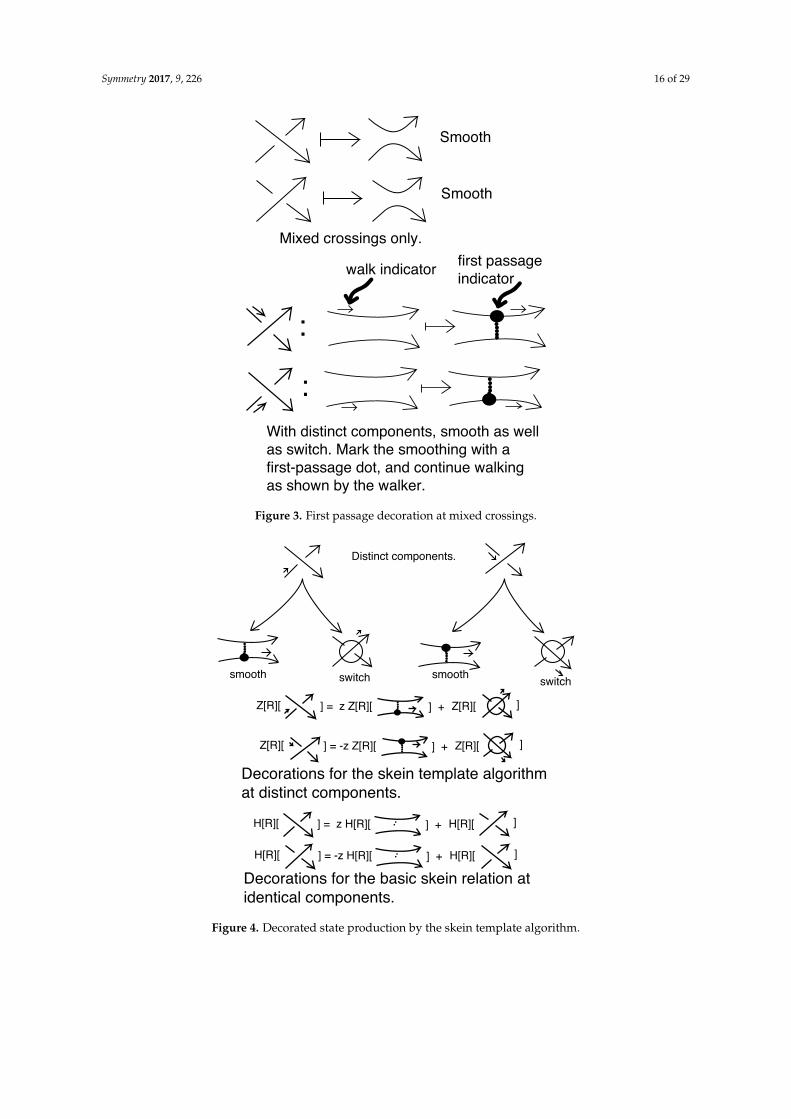
Definition 1. Let L denote a diagram of an oriented link. The oriented smoothing of a crossing is the replacementof the crossing by the smoothing that is consistent with the orientations of its two arcs. See Figure 3 top.Pre-states, S, for L are obtained by successively smoothing or switching mixed crossings (a mixed crossing is acrossing between two components of the link). That is, one begins by choosing a mixed crossing and replacingit by smoothing it and switching it, see Figure 4 top. The smoothing is decorated as in Figure 3, so that thereis a dot that discriminates whether the smoothing comes from a positive or a negative crossing. The process ofplacing the dot is related to walking along the diagram. That walk only allows a smoothing at a mixed crossingthat is approached along an undercrossing arc as shown in Figure 3. After the smoothing is produced, that walkand the dotting are related as shown in Figure 3. The reasons for these conventions will be clarified below, wherewe explain a process that encodes the skein calculation of the invariants. The switched crossing is circled toindicate that it has been chosen by this skein process, see Figure 5. Then one chooses another mixed crossing ineach of the resulting diagrams and applies the same procedure. New self-crossings can appear after a smoothing.A completed pre-state is obtained when a decorated diagram is reached where all the undecorated crossings areself-crossings. A state, S, for L is a completed pre-state that is obtained with respect to a template as we describeit below. In a state, we are guaranteed that the resulting link diagram is a topological union of unlinked knotdiagrams (a stack). In fact, the skein template process will produce exactly a set of states whose evaluationscorrespond to the skein evaluation of the invariant H[R].

In the skein template algorithm we produce a specific set of pre-states that we can call states, andshow how to compute the link invariant H[R] from these states by adding up evaluations of each state.The key to producing these pre-states is the template. A template, T, for a link diagram L is an indexed,flattened diagram for L (the underlying universe of L, a 4-valent graph obtained from L by ignoringthe over and under crossing data in L) so that the indices are on the edges of the graph. See Figure 6 foran illustration of a template T for the Hopf link. We assume that the indices are distinct elements of anordered set (for example, the natural numbers). We use the template to decide the order of processingfor the pre-state. As we know, the invariant H[R] itself is independent of this ordering. Take the linkdiagram L and a template T for L. Process the diagram L to produce pre-states S generated by thetemplate T by starting at the smallest index and walking along the diagram, smoothing and markingas described below.

Symmetry 2017, 9, 226 16 of 29

walk indicator first passage indicator

:

:

Smooth

Smooth

Mixed crossings only.

With distinct components, smooth as wellas switch. Mark the smoothing with a first-passage dot, and continue walking as shown by the walker.

Figure 3. First passage decoration at mixed crossings.

Distinct components.

smooth switch

] = z Z[R][ ] + Z[R][ ]Z[R][

] = z H[R][ ] + H[R][ ]H[R][

] = -z H[R][ ] + H[R][ ]H[R][

Decorations for the skein template algorithmat distinct components.

Decorations for the basic skein relation atidentical components.

] = -z Z[R][ ] + Z[R][ ]Z[R][

smooth switch

Figure 4. Decorated state production by the skein template algorithm.

Symmetry 2017, 9, 226 17 of 29

In a mixed crossing an approach at an undercrossing switchesthe crossing from diagram to state.

:

:

For a same component crossing,retain the crossing in the orginal diagramfor both approached at either an under oran overcrossing, and do not circle the crossing.

:

In a mixed crossing an approachat an overcrossing retains the crossing type.

:

Figure 5. Decorations on walking past a crossing in a pre-state.

12

34

S State S from S and the template T.

T

S S'

State S' from template T.

Figure 6. State production for the Hopf link.

5.1. The Skein Template Algorithm

The skein template algorithm is basically very simple. It is a formalization of the skein calculationprocess, designed to fix all the choices in this process by the choice of the template T. Then the resultingstates are exactly the ends of a skein tree for evaluating H[R]. Each state, as a link diagram, is a stack

Symmetry 2017, 9, 226 18 of 29

of knots, ready to be evaluated by R. The product of the vertex weights for the state multiplied by Revaluated on the state is equal to the contribution of that state to the polynomial.

We now detail the skein template algorithm. Consider a link diagram L (view Figures 6 and 7).Label each edge of the projected flat diagram of L from an ordered index set I so that each edge receivesa distinct label. We have called this labeled graph the template T(L). We have defined a pre-state Sof L by selecting mixed crossings in L and operating on them according to a walk on the template,starting with the smallest index in the labeling of T. We now go through the skein template algorithm,referring at the same time to specific examples.

1. Begin walking along the link L, starting at the least available index from T(L). See Figures 6 and 7.2. When meeting a mixed crossing via an under-crossing arc, produce two new diagrams

(see Figure 4 top), one by switching the crossing and circling it (Figure 5) and one by smoothingthe crossing and labeling it (Figure 3).

3. When traveling through a smoothing, label it by a dot and a connector indicating the place of firstpassage as shown in Figure 3 and exemplified in Figures 6 and 7. At a smoothing, assign to thesmoothing a vertex weight of +z or −z (the weights are indicated in Figure 8).

We clarify these steps with two examples, the Hopf link and the Whitehead link.See Figures 6 and 7. In these figures, for Step 1 we start at the edge with index 1 and meeta mixed crossing at its under-arc, switching it for one diagram and smoothing it for another. Wewalk past the smoothing, placing a dot and a connector.

4. When meeting a mixed over-crossing, circle the crossing (Figure 5 middle) to indicate that it hasbeen processed and continue the walk.

5. When meeting a self-crossing, leave it unmarked (Figure 5 bottom) and continue the walk.6. When a closed path has been traversed in the template, choose the next lowest unused template

index and start a new walk. Follow the previous instructions for this walk, only labelingsmoothings or circling crossings that have not already been so marked.

7. When all paths have been traversed, and the pre-state has no remaining un-processed mixedcrossing, the pre-state S is now a state S for L. When we have a state S, it is not hard to see thatit consists in an unlinked collection of components in the form of stacks of knots as we havepreviously described in this paper.

8. When a pre-state is finished, there will be no undecorated mixed crossings in the state.All uncircled crossings will be self-crossings and there will also be some marked smoothings.All the smoothings will have non-zero vertex weights ( z, −z or 1) and the pre-state becomes acontributing state for the invariant.

9. This state is evaluated by taking the product of the vertex weights and the evaluation of theinvariant R on the the link underlying the state after all the decorations have been removed.The skein template process produces a link from the state that is a stack of knots. We give thedetails in the next section.

10. The (unnormalized) invariant H[R] is the sum over all the evaluations of these states obtained byapplying the skein-template algorithm. We will denote this sum by Z[R](L) for a given link Land justify in the discussion below that it is indeed equal to the previously defined H[R](L).

Returning to our example, we have the diagram shown in Figure 6. In this diagram S is acompleted state for the initial link L. Note that in forming S we start at 1 in the template and firstencounter a mixed under-crossing. This is smoothed to produce the pre-state S, and the walk continuesto encounter a self-crossing that is left alone. The result is the state S. Moreover, first encounter from1 meets an under-crossing and we switch and circle this crossing and continue that walk. The nextcrossing is an over-crossing that is mixed. We circle this crossing and produce the state S′. The twostates S and S′ are a complete set of states produced by the skein template algorithm for the Hopf linkL with this template T.

Symmetry 2017, 9, 226 19 of 29

12

3

4

5

6

7

891011

12

L

T(L)

S1

S2 S3

Figure 7. Skein template algorithm applied to the Whitehead link.

||

||

[[

[[]

] ]]= z

= 0 = -z

= 0

[ [

[ [

] ]

] ]| |

| | =

=

=

=

1

1

Figure 8. State evaluation relative to the diagram L.

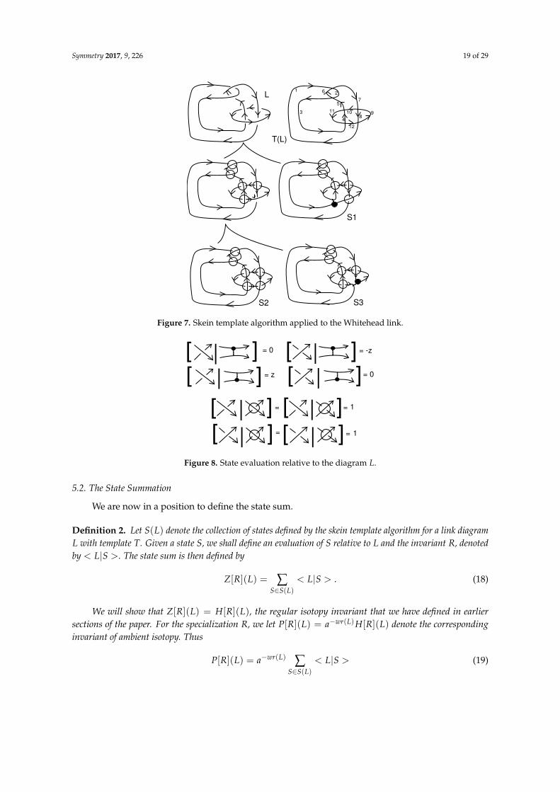
5.2. The State Summation

We are now in a position to define the state sum.

Definition 2. Let S(L) denote the collection of states defined by the skein template algorithm for a link diagramL with template T. Given a state S, we shall define an evaluation of S relative to L and the invariant R, denotedby < L|S >. The state sum is then defined by

Z[R](L) = ∑S∈S(L)

< L|S > . (18)

We will show that Z[R](L) = H[R](L), the regular isotopy invariant that we have defined in earliersections of the paper. For the specialization R, we let P[R](L) = a−wr(L)H[R](L) denote the correspondinginvariant of ambient isotopy. Thus

P[R](L) = a−wr(L) ∑S∈S(L)

< L|S > (19)

Symmetry 2017, 9, 226 20 of 29

gives the normalized invariant of ambient isotopy in state sum form. The sites of the state S consist in thedecorated smoothings and the decorated crossings indicated in Figure 4. Each state evaluation < L|S > consistsof two parts. We shall write it in the form

< L|S >= [L|S][R|S]. (20)

The first part [L|S] depends only on L and the state S. The second part [R|S] uses the chosen knot invariantR. We define [L|S] as a product over the sites of S:

[L|S] = ∏σ∈sites(S)

[L|σ] (21)

where [L|σ] is defined by the equations in Figure 8, comparing a crossing in L with the corresponding site σ.This means that if a smoothed site has a dot along its lower edge (when oriented from left to right), then its vertexweight is +z and if it has a dot along its upper edge, then it has a vertex weight −z. Circled crossings havevertex weights 1. In Figure 8 we have indicated the possibility of vertex weights 0, but these will never occur inthe states produced by the skein template algorithm. If we were to sum over a larger set of states, then some ofthem would be eliminated by this rule. The reader should note that the choice of +z or −z is directly in accordwith the rules for the skein relation from a positive crossing or a negative crossing, respectively. We define [R|S]as a weighted product of the R-evaluations of the components of the state S:

[R|S] = [k

∏i=1

ρ(Ki)]E1−k (22)

where E is defined previously and

ρ(K) = awr(K)R(K).

Here {K1, . . . , Kk} is the set of component knots of the state S. Recall that each state S is a stacked union ofsingle unlinked component knots Ki, i = 1, . . . , k, with k depending on the state. In computing ρ(Ki) we ignorethe state decorations and remove the circles from the crossings. With this, we have completed the definition of thestate sum.

Note that, by (18) and (20) we assert that

Z[R](L) = ∑S∈S(L)

[L|S][R|S]. (23)

Remark 6. If the invariant R is itself generated by a state summation, then we obtain a hybrid state sum forZ[R](L) consisting in the concatenations (in order) of these two structures. We expand on this idea in Section 6.

5.3. Connection of the State Sum with Skein Calculation

We will show that the sum over states corresponds exactly with the results of making a skeincalculation that is guided by the template in the skein template algorithm. Thus the template that wehave already described works in these two related contexts. In this way we will show that the statesummation gives a formula for the invariant H[R](L).

We begin with an illustration for a single abstract crossing as shown in Figure 5. We shall referto the skein calculation guided by the template as the skein algorithm. In this figure the walker in theskein algorithm (using the template) approaches along the under-crossing line. If the crossing that ismet is a self-crossing of the given diagram, then the walker just continues and the crossing is circled.If the crossing that is a mixed crossing of the given diagram, then two new diagrams are produced.In the first case we produce a smoothing with the labelling that indicates a passage along the edgemet from the undercrossing arc. In the second case the walker switches the crossing and continues in

Symmetry 2017, 9, 226 21 of 29

the same direction as shown in the figure. This creates a bifurcation in the skein tree. Each resultingbranch of the skein tree is treated recursively in this way, but first the walker continues on these givenbranches until it meets an undercrossing of two different components. Using the Homflypt regularisotopy skein relation (recall Theorem 1, rule (1)) we can write an expansion symbolically as shown inFigure 4. Here it is understood that in expanding a crossing,

1. its two arcs lie on separate components of the given diagram;2. the walker for the skein process always switches a mixed crossing that the walker approaches as

an under-crossing, and never switches a crossing that it approaches as an over-crossing;3. in expanding the crossing, the walker is shifted along according to the illustrations in Figure 4.

Thus, for different components, we have the expansion equation shown in Figure 4. Here, thetemplate takes on the role of letting us make a skein tree of exactly those states that contribute tothe state sum for Z[H](L). Indeed, examine Figure 8. The zero-weights correspond to inadmissiblestates while the z and −z weights correspond to admissible states where the walker approached atan under-crossing; the one-weights correspond to any circled crossing. Thus, we can use the skeinalgorithm to produce exactly those states that have a non-zero contribution to the state sum.

By using the skein template algorithm and the skein formulas for expansion, we produce a skeintree where the states at the ends of the tree (the original link is the root of the tree) are exactly the statesS that give non-zero weights for [L|S]. Thus, by (18) we obtain:

Z[R](L) = ∑S∈Ends(SkeinTree)

< L|S > . (24)

Since we have shown that the state sum is identical with the skein algorithm for computingH[R](L), for any link L, this shows that Z[R](L) = H[R](L), as promised. Thus, we have proved:

Theorem 8. The state sum we have defined as Z[R](L) is identical with the skein evaluation of the invariantH[R](L). We conclude that Z[R](L) = H[R](L), and thus that the skein template algorithm provides a statesummation model for the invariant H[R](L).

Proof. The state sum Z[R](L) = ∑S∈S(L) < L|S > where S(L) denotes all the states produced by theskein template algorithm, for a choice of template T. Z[R](L) is equal to the sum of evaluations ofthose states that are produced by the skein algorithm. That is we have the identity

Z[R](L) = ∑S∈S(L)

< L|S >= ∑S∈Ends(SkeinTree)

< L|S >= H[R](L).

The latter part of this formula follows because the skein template algorithm is a description of aparticular skein calculation process for H[R](L), that is faithful to the rules and weights for H[R](L).We have also proved that H[R](L) is invariant and independent of the skein process that producesit. Thus we conclude that Z[R](L) = H[R](L), and thus that the skein template algorithm provides astate summation model for the invariant H[R](L).

Remark 7. Note that it follows from the proof of Theorem 8 that the calculation of Z[R](L) = H[R](L) isindependent of the choice of the template for the skein template algorithm.

Example 2. In the example shown in Figure 7 we apply the skein template algorithm to the Whitehead link L.The skein-tree shows that for the given template T there are three contributing states S1, S2, S3. S1 is a knot K.S2 is a stacked unlink or two unknotted components. S3 is an unknot. Thus, referring to Figure 9 and using (19)we find the calculation shown below.

Z[R](L) = z[R|S1] + [R|S2]− z[R|S3]

Symmetry 2017, 9, 226 22 of 29

= zR(K) + a−2(η/E)− za−3,

where η = (a− a−1)/w is defined in rule (5) after Theorem 1 and K = S1.

Remark 8. In the example above we see that any choice of specialization for the invariant R that can distinguishthe trivial knot from the trefoil knot K will suffice for our invariant to distinguish the Whitehead link from thetrivial link, for which Z[R](©©) = η/E.

L

S1

S2

S3

z

-z

~

K

~

Figure 9. States for the Whitehead link.

6. Double State Summations

In this section, we consider state summations for our invariant where the invariant R has a statesummation expansion. The invariant R has a variable w and a framing variable a. By choosing thesevariables in particular ways, we can adjust R to be the usual regular isotopy Homflypt polynomial orspecializations of the Homflypt polynomial such as a version of the Kauffman bracket polynomial,or the Alexander polynomial, or other invariants. We shall refer to these choices as specializations ofR. A given specialization of R may have its own form of state summation. This can be combinedwith the skein template algorithm that produces states to be evaluated by R. The result is a doublestate summation.

As in the previous section we have the global state summation (23):

Z[R](L) = ∑S∈S(L)

[L|S][R|S]

where [R|S] denotes the evaluation of the invariant R on the union of unlinked knots that is theunderlying topological structure of the state S. It is possible that the specialization we are using hasitself a state summation that is of interest. In this case we would have a secondary state summationformula of the type

[R|S] = ∑σ

[S|σ]. (25)

Symmetry 2017, 9, 226 23 of 29

Then, we would have a double state summation for the entire invariant in the schematic form:

Z[R](L) = ∑S∈S(L),σ∈Rstates(S)

[L|S][S|σ], (26)

where Rstates(S) denotes the secondary states for R of the union of unlinked knots that underlies thestate S.

Example 3. Since we use the skein template algorithm to produce the first collection of states S ∈ S(L),this double state summation has a precedence ordering with these states produced first, then each S is viewed as astack of knots and the second state summation is applied. In this section, we will discuss some examples for statesummations for R and then give examples of using the double state summation.

We begin with a state summation for the bracket polynomial that is adapted to our situation. View Figure 10.At the top of the figure we show the standard oriented expansion of the bracket. If the reader is familiar withthe usual unoriented expansion [39], then this oriented expansion can be read by forgetting the orientations.The oriented states in this state summation contain smoothings of the type illustrated in the far right hand termsof the two formulas at the top of the figure. We call these disoriented smoothings since two arrowheads pointto each other at these sites. Then by multiplying the two equations by A and by A−1 respectively, we obtain adifference formula of the type

A < K+ > −A−1 < K− >= (A2 − A−2) < K0 >

where K+ denotes the local appearance of a positive crossing, K− denotes the local appearance of a negativecrossing and K0 denotes the local appearance of standard oriented smoothing. The difference equation eliminatesthe disoriented terms. It then follows easily from this difference equation that if we define a curly bracket bythe equation

{K} = Awr(K) < K >

where wr(K) is the diagram writhe (the sum of the signs of the crossings of K), then we have a Homflypt typerelation for {K} as follows:

{K+} − {K−} = (A2 − A−2){K0}. (27)

This means that we can regard {K} as a specialization of the Homflypt polynomial and so we can use it asthe invariant R in our double state summation. The state summation for {K} is essentially the same as that forthe bracket, as we now detail.

< >

< >

< > < >= A A-1

+

< > < >A A-1

+=

{ }

{K} = A <K>wr(K)

Define

< > < >A - A-1

(A - A2 -2

) < >

=

- (A - A2 -2

)= { }{}

.

Figure 10. Oriented bracket with Homflypt skein relation.

From Figure 10 it is not difficult to see that

{K+} = A2{K0}+ {K∞} (28)

Symmetry 2017, 9, 226 24 of 29

and{K−} = A−2{K0}+ {K∞}. (29)

Here K∞ denotes the disoriented smoothing shown in the figure. These formulas then define thestate summation for the curly bracket. The reader should note that the difference of these two expansionEquations (28) and (29) is the difference formula (27) for the curly bracket in Homflypt form. The correspondingstate summation [40] for these equations is

{K} = ∑σ

A2s+(σ)−2s−(σ)(−A2 − A−2)||σ||−1,

where σ runs over all choices of oriented and disoriented smoothings of the crossings of the diagram K. Here s+(σ)denotes the number of oriented smoothings of positive crossings and s−(σ) denotes the number of orientedsmoothings of negative crossings in the state σ. Further, ||σ|| denotes the number of loops in the state σ.

With this state sum model in place we can proceed to write a double state sum for the bracket polynomialspecialization of our invariant. The formalism of this invariant is after (26), as follows.

Z[{ }](L) = ∑S∈S(L)

[L|S]{S} = ∑S∈S(L)

∑σ∈smoothings(S)

[L|S]A2s+(σ)−2s−(σ)(−A2 − A−2)||σ||−1. (30)

Here we see the texture of the double state summation. The skein template algorithm produces from theoriented link L the stacks of knots K. Each such stack has a collection of smoothing states, and for each suchsmoothing state we have the term in the curly bracket expansion formula multiplying a corresponding term fromthe skein template expansion.

There are many other examples of specific double state summations for other choices of thespecialization of the Homflypt polynomial.

Example 4. For example, we can use the specialized Homflypt state summation based on a solution to theYang-Baxter equation as explained in [39,40,43].

Example 5. We could also take the specialization to be the Alexander–Conway polynomial and use the FormalKnot Theory state summation as explained in [44].

All these different cases deserve more exploration, particularly for computing examples of thesenew invariants.

Remark 9. The skein template algorithm as well as the double state summation generalizes to the Dubrovnikand Kauffman polynomials, and so applies to our generalizations of them, D[D] and K[K], as well. We will takeup this computational and combinatorial subject in a sequel to the present paper.

Remark 10. Consider the combinatorial formula (7). This formula can be regarded itself as a state summation,where the states are the partitions π and the state evaluations are given by the formula and the evaluations ofthe regular isotopy Homflypt polynomial R on πL. If we choose a state summation for R or a specialization ofR, then this formula becomes a double state summation in the same sense as we discussed above, but withoutusing the skein template algorithm. These double state sums deserve further investigation both for H[R]and also for the counterparts (15) and (16) for the generalizations D[D] and K[K] of the Kauffman and theDubrovnik polynomials.

Symmetry 2017, 9, 226 25 of 29

7. Statistical Mechanics and Double State Summations

In statistical mechanics, one considers the partition function for a physical system [45]. The partitionfunction ZG(T) is a summation over the states σ of the system G:

ZG = ∑σ

e−1kT E(σ)

where T is the temperature and k is Bolztmann’s constant. Combinatorial models for simplifiedsystems have been studied intensively since Onsager [46] showed that the partition function for theIsing model for the limits of planar lattices exhibits a phase transition. Onsager’s work showed thatvery simple physical models, such as the Ising model, can exhibit phase transitions, and this ledto the deep research subject of exactly solvable statistical mechanics models [45]. The q-state Pottsmodel [45,47] is an important generalization of the Ising model that is based on q local spins at each sitein a graph G. For the Potts model, a state of the graph G is an assignment of spins from {1, . . . , q} toeach of the nodes of the graph G. If σ is such a state and i denotes the i-th node of the graph G, then welet σi denote the spin assignment to this node. Then the energy of the state σ is given by the formula

E(σ) = ∑〈i,j〉

δ(σi, σj)

where 〈i, j〉 denotes an edge in the graph between nodes i and j, and δ(x, y) is equal to 1 when x = yand equal to 0 otherwise.

Temperley and Lieb [48] proved that the partition function for the Potts model can be calculatedusing a contraction—deletion algorithm, and so showed that ZG is a special version of the dichromaticor Tutte polynomial in graph theory. This, in turn, is directly related to the bracket polynomial statesum, and so by generalizing the variables in the bracket state sum and translating the planar graphG into a knot diagram by a medial construction (associating a planar graph to a link diagram via acheckerboard coloring of the diagram so that each shaded region in the checkerboard corresponds to agraphical node and each crossing between shaded regions corresponds to an edge) , one obtains anexpression for the Potts model as a bracket summation with new parameters [47]. We wish to discussthe possible statistical mechanical interpretation of our generalized bracket state summation Z[{ }](see Equation (30)). In order to do this we shall extend the variables of our state sum so that the bracketcalculation (for the stacks of knots S that correspond to skein template states) is sufficiently general tosupport (generalized) Potts models associated with these knots. Accordingly, we add variables to thebracket expansion so that

{K+} = x{K0}+ y{K∞},

{K−} = x′{K0}+ y′{K∞}

and the loop value is taken to be D rather than −A2 − A−2.For a given knot in the stack S, the state sum remains well-defined and it now can be

specialized to compute a generalized Potts model for a plane graph via a medial graph translation.Letting R(K) = {K} denote this bracket state sum, we can then form a generalized version of Z[R]by using the expansion in Figure 11 where we use the raw states of this figure, and we do not filterthem by the skein template algorithm, but simply ask that each final state is a union of unlinkedknots. The result will then be a combinatorially well-defined double-tier state sum. It is this state sumZ[R] that can be examined in the light of ideas and techniques in statistical mechanics. The first tierexpansion is highly non-local, and just pays attention to dividing up the diagrams so that the first tierof states are each collections of unlinked knots. Then each knot can be regarded as a localized physicalsystem and evaluated with the analogue of a Potts model. This is the logical structure of our doublestate summation, and it is an open question whether it has a significant physical interpretation.

Symmetry 2017, 9, 226 26 of 29

Distinct components.

smooth switch

] = z Z[R][ ] + Z[R][ ]Z[R][

] = -z Z[R][ ] + Z[R][ ]Z[R][

Summary of the Skein Template Algorithm

Expand by these rules for positive and negative crossings of distinct components. Note that when a crossing is smoothed, the local distinctions of same and different components changes.Crossings are smoothed and marked with a dot,or switched and marked with a circle. This providesraw states (containing only self-crossings) that are then filteredby the choice of template in the algorithm and further evaluated. The resulting disjoint collections of knots are evaluatedby R. For a statistical mechanics model, we keep all raw states thatare disjoint unions of knot diagrams.

Figure 11. Raw state production for skein template algorithm.

8. Discussing Applications

We contemplate how these new ideas can be applied to physical situations. We present theseindications of possible applications here with the full intent to pursue them in subsequent publications.

1. Reconnection (in vortices). In a knotted vortex in a fluid or plasma (for example in solar flares) [49]one has a cascade of changes in the vortex topology as strands of the vortex undergo reconnection.The process goes on until the vortex has degenerated into a disjoint union of unknotted simplervortices. This cascade or hierarchy of interactions is reminiscent of the way the skein templatealgorithm proceeds to produce unlinks. Studying reconnection in vortices may be facilitatedby making a statistical mechanics summation related to the cascade. Such a summation will beanalogous the state summations we have described here.

2. In DNA, strand switching using topoisomerase of types I and II is vital for the structure ofDNA replication [50]. The mixed interaction of topological change and physical evolution of themolecules in vitro may benefit from a mixed state summation that averages quantities respectingthe hierarchy of interactions.

3. Remarkably, the process of separation and evaluation that we have described here is analogous toproposed processing of Kinetoplast DNA [51] where there are huge links of DNA circles and thesemust undergo processes that both unlink them from one another and produce new copies foreach circle of DNA. The double-tiered structure of DNA replication for the Kinetoplast chainmailDNA appears to be related to the mathematical patterns of our double state summations. If thereader examines the Wiki on Kinetoplast DNA, he/she will note that Topoisomerase II figurescrucially in the self-replication [52].

4. We wondered whether we could have physical situations that would have the kind of a mixturethat is implicit in this state summation, where the initial skein template state sum yields a sumover R-evaluations, and R may itself have a state summation structure. One possible example in

Symmetry 2017, 9, 226 27 of 29

the physical world is a normal statistical mechanical situation, where one can have multiple typesof materials, all present together, each having different energetic properties. This can lead to amixed partition function, possibly not quite ordered in the fashion of our algorithm. This wouldinvolve a physical hierarchy of interactions so that there would be a double (or multiple) tierresulting from that hierarchy.

5. Mixed state models can occur in physical situations when we work with systems of systems.There are many examples of this multiple-tier situation in systems physical and biological. We lookfor situations where a double state sum would yield new information. For example, in a quantumHall system [53], the state of the system is in its quasi-particles, but each quasi-particle is itself avortex of electrons related to a magnetic field line. So the quasi-particles are themselves localizedphysical systems. Some of this is summarized in the Laughlin wave function for quantumHall [53]. This is not a simple situation, but a very significant one. There should be otherimportant examples.

9. Conclusions

We have generalized the known skein polynomials to new and more powerful invariants of linksby adopting a new two-level skein procedure. We have shown that these new invariants can also beachieved by special formulas evaluating the original invariants on collections of sublinks of the giveninitial link. We then show how our new skeining procedure leads to state summation expressions forthe invariants and how, if the original invariant is given by a state sum, the new state sums are doublelevel state sums involving a mixture of the two forms of summation. This leads to considerations ofstatistical mechanics models and also physical and biological processes that have significant multiplelevels. We conclude that this way of working with skein invariants has the potential to lead to newinsights into physical and biological processes.

Acknowledgments: The first-listed author is pleased to acknowledge support from his Simons FoundationCollaboration Grant for Mathematicians, Award Number 426075. Both authors are pleased to acknowledge theMathematisches Forschungsinstitut Oberwolfach for their hospitality and support during the preparation ofthis research.

Author Contributions: The authors contributed equally to this work.

Conflicts of Interest: The authors declare no conflict of interest.

References

1. Kauffman, L.H.; Lambropoulou, S. New invariants of links and their state sum models. arXiv 2017,arXiv:1703.03655.

2. Alexander, J.W. Topological invariants of knots and links. Trans. Am. Math. Soc. 1928, 30, 275–306.3. Conway, J.H. An enumeration of knots and links and some of their algebraic properties. In Computational

Problems in Abstract Algebra, Proceedings of the Conference Held at Oxford under the Auspices of the Science ResearchCouncil Atlas Computer Laboratory, Oxford, UK, 29 August–2 September 1967; Pergamon: Oxford, UK, 1970;pp. 329–358.

4. Jones, V.F.R. A polynomial invariant for knots via von Neumann algebras. Bull. Am. Math. Soc. (N.S.) 1985,12, 103–111.

5. Jones, V.F.R. Hecke algebra representations of braid groups and link polynomials. Ann. Math. 1987, 126, 335–388.6. Lickorish, W.B.R.; Millett, K.C. A polynomial invariant of oriented links. Topology 1987, 26, 107–141.7. Freyd, P.; Yetter, D.; Hoste, J.; Lickorish, W.B.R.; Millett, K.C.; Ocneanu, A. A new polynomial invariant of

knots and links. Bull. AMS 1985, 12, 239–246.8. Przytycki, J.H.; Traczyk, P. Invariants of links of Conway type. Kobe J. Math. 1987, 4, 115–139.9. Kauffman, L.H. State models and the Jones polynomial. Topology 1987, 26, 395–407.10. Brandt, R.D.; Lickorish, W.B.R.; Millett, K.C. A polynomial invariant for unoriented knots and links.

Invent. Math. 1986, 84, 563–573.11. Kauffman, L.H. An invariant of regular isotopy. Trans. Am. Math. Soc. 1990, 318, 417–471.

Symmetry 2017, 9, 226 28 of 29

12. Juyumaya, J.; Lambropoulou, S. p–adic framed braids II. Adv. Math. 2013, 234, 149–191.13. Chlouveraki, M.; Juyumaya, J.; Karvounis, K.; Lambropoulou, S. Identifying the invariants for classical knots

and links from the Yokonuma-Hecke algebra. arXiv 2016, arXiv:1505.06666.14. Juyumaya, J. Markov trace on the Yokonuma-Hecke algebra. J. Knot Theory Ramif. 2004, 13, 25–39.15. Juyumaya, J.; Lambropoulou, S. An adelic extension of the Jones polynomial. In The Mathematics of Knots;

Banagl, M., Vogel, D., Eds.; Contributions in the Mathematical and Computational Sciences; Springer:New York, NY, USA, 2009; Volume 1, pp. 825–840.

16. Chlouveraki, M.; Lambropoulou, S. The Yokonuma-Hecke algebras and the Homflypt polynomial. J. KnotTheory Ramif. 2013, 22, 1350080.

17. Chmutov, S.; Jablan, S.; Karvounis, K.; Lambropoulou, S. On the knot invariants from the Yokonuma–Heckealgebras. J. Knot Theory Ramif. 2016, 25, 1641004.

18. Karvounis, K. Enabling computations for link invariants coming from the Yokonuma-Hecke algebras. J. KnotTheory Ramif. 2016, 25, 1641012.

19. Chlouveraki, M.; Poulain d’Andecy, L. Representation theory of the Yokonuma–Hecke algebra. Adv. Math.2014, 259, 134–172.

20. Aicardi, F.; Juyumaya, J. Tied Links. J. Knot Theory Ramif. 2016, 25, 1641001.21. Karvounis, K.; Lambropoulou, S. Link invariants from the Yokonuma-Hecke algebras. In Algebraic Modeling

of Topological and Computational Structures and Applications; Lambropoulou, S., Stefaneas, P., Theodorou, D.,Kauffman, L.H., Eds.; Springer Proceedings in Mathematics & Statistics (PROMS); THALES Workshop:Athens, Greece, 2015, to appear November 2017.

22. Juyumaya, J.; Lambropoulou, S. An invariant for singular knots. J. Knot Theory Ramif. 2009, 18, 825–840.23. Juyumaya, J.; Lambropoulou, S. Modular framization of the BMW algebra. arXiv 2010, arXiv:1007.0092v1.24. Juyumaya, J.; Lambropoulou, S. On the framization of knot algebras. In New Ideas in Low-Dimensional Topology;

Kauffman, L.H., Manturov, V. O., Eds.; Series on Knots and Everything; World Scientific: Singapore, 2014.25. Goundaroulis, D. Framization of the Temperley-Lieb Algebra and Related Link Invariants. Ph.D. Thesis,

Department of Mathematics, National Technical University of Athens, Athens, Greece, 2014.26. Goundaroulis, D.; Juyumaya, J.; Kontogeorgis, A.; Lambropoulou, S. The Yokonuma–Temperley–Lieb

algebra. Banach Center Pub. 2014, 103, 73–95.27. Chlouveraki, M.; Pouchin, G. Determination of the representations and a basis for the

Yokonuma–Temperley–Lieb algebra. Algebras Represent. Theory 2015, 18, 421–447.28. Goundaroulis, D.; Juyumaya, J.; Kontogeorgis, A.; Lambropoulou, S. Framization of the Temperley–Lieb

algebra. Math. Res. Lett. 2017, 24, 299–345.29. Chlouveraki, M.; Pouchin, G. Representation theory and an isomorphism theorem for the Framisation of the

Temperley–Lieb algebra. arXiv 2015, arXiv:1503.03396v2.30. Jacon, N.; Poulain d’Andecy, L. An isomorphism theorem for Yokonuma–Hecke algebras and applications to

link invariants. Math. Z. 2016, 283, 301–338.31. Goundaroulis, D.; Lambropoulou, S. Classical link invariants from the framizations of the Iwahori–Hecke

algebra and the Temperley–Lieb algebra of type A. J. Knot Theory Ramif. 2017, 26, 1743005.32. Juyumaya, J. A partition Temperley–Lieb algebra. arXiv 2013, arXiv:1304.5158.33. Goundaroulis, D.; Lambropoulou, S. A new two-variable generalization of the Jones polynomial. arXiv 2016,

arXiv:1608.01812.34. Poulain d’Andecy, L.; Wagner, E. The HOMFLYPT polynomials of sublinks and the Yokonuma–Hecke

algebras. arXiv 2016, arXiv:1606.00237v1.35. Aicardi, F.; Juyumaya, J. Markov trace on the algebra of braids and ties. Moscow Math. J. 2016, 16, 397–431.36. Aicardi, F.; Juyumaya, J. Kauffman type invariants for tied links. arXiv 2016, arXiv:1607.04841.37. Chlouveraki, M.; Poulain d’Andecy, L. Markov trace on affine and cyclotomic Yokonuma–Hecke algebras.

Int. Math. Res. Notices 2016, 14, 4167–4228, doi:10.1093/imrn/rnv257.38. Flores, M.; Juyumaya, J.; Lambropoulou, S. A Framization of the Hecke algebra of Type B. J. Pure Appl. Algebra

2017, doi:10.1016/j.jpaa.2017.05.006.39. Kauffman, L.H. State models for link polynomials. Enseign. Math. 1990, 36, 1–37.40. Kauffman, L.H. Knots and Physics, 4th ed.; Series on Knots and Everything 53; World Scientific Publishing Co.

Pte. Ltd.: Hackensack, NJ, USA, 2013.41. Thistlethwaite, M. Links with trivial Jones polynomial. J. Knot Theory Ramif. 2001, 10, 641–643.

Symmetry 2017, 9, 226 29 of 29

42. Eliahou, S.; Kauffman, L.H.; Thistlethwaite, M.B. Infinite families of links with trivial Jones polynomial.Topology 2003, 42, 155–169.

43. Jones, V.F.R. On knot invariants related to some statistical mechanical models. Pac. J. Math. 1989, 137, 311–334.44. Kauffman, L.H. Formal Knot Theory; Lecture Notes Series No. 30; Princeton University Press:

Princeton, NJ, USA, 1983.45. Baxter, R.J. Exactly Solved Models in Statistical Mechanics; Academic Press: London, UK, 1982.46. Onsager, L. Crystal statistics. I. A two-dimensional model with an order-disorder transition. Phys. Rev. 1944,

65, 117–149.47. Kauffman, L.H. Statistical Mechanics and the Jones Polynomial. In Braids; Contemporary Mathematics;

American Mathematical Society: Providence, RI, USA, 1988; Volume 78, pp. 263–297.48. Temperley, H.N.V.; Lieb, E.H. Relations between the “percolation” and “colouring” problem and other

graph-theoretical problems associated with regular planar lattices: Some exact results for the “percolation”problem. Proc. R. Soc. Lond. Ser. A 1971, 322, 251–280.

49. Scheeler, M.W.; Kleckner, D.; Proment, D.; Kindlmann, G.L.; Irvine, W.T.M. Helicity conservation by flowacross scales in reconnecting vortex links and knots. arXiv 2014, arXiv:1404.6513.

50. Ernst, C.; Sumners, D.W. Solving tangle equations arising in a DNA recombination model. Math. Proc. Camb.Philos. Soc. 1999, 126, 23–36.

51. Michieletto, D.; Marenduzzo, D.; Turner, M.S. Topology Regulation during Replication of the KinetoplastDNA. arXiv 2014, arXiv:1408.4237.

52. Kinetoplast. Available online: https://en.wikipedia.org/wiki/Kinetoplast (accessed on 3 March 2017).53. Johri, S.; Papic, Z.; Schmitteckert, P.; Bhatt, R.N.; Haldane, F.D.M. Probing the geometry of the Laughlin state.

arXiv 2015, arXiv:1512.08698.

c© 2017 by the authors. Licensee MDPI, Basel, Switzerland. This article is an open accessarticle distributed under the terms and conditions of the Creative Commons Attribution(CC BY) license (http://creativecommons.org/licenses/by/4.0/).