DI

SC

US

SI

ON

P

AP

ER

S

ER

IE

S

Forschungsinstitut zur Zukunft der ArbeitInstitute for the Study of Labor

Lost in Transition? Minimum Wage Effects onGerman Construction Workers

IZA DP No. 6760

July 2012

Ronald BachmannMarion KönigSandra Schaffner

Lost in Transition? Minimum Wage

Effects on German Construction Workers

Ronald Bachmann RWI and IZA

Marion König

IAB

Sandra Schaffner RWI

Discussion Paper No. 6760 July 2012

IZA

P.O. Box 7240 53072 Bonn

Germany

Phone: +49-228-3894-0 Fax: +49-228-3894-180

E-mail: iza@iza.org

Any opinions expressed here are those of the author(s) and not those of IZA. Research published in this series may include views on policy, but the institute itself takes no institutional policy positions. The Institute for the Study of Labor (IZA) in Bonn is a local and virtual international research center and a place of communication between science, politics and business. IZA is an independent nonprofit organization supported by Deutsche Post Foundation. The center is associated with the University of Bonn and offers a stimulating research environment through its international network, workshops and conferences, data service, project support, research visits and doctoral program. IZA engages in (i) original and internationally competitive research in all fields of labor economics, (ii) development of policy concepts, and (iii) dissemination of research results and concepts to the interested public. IZA Discussion Papers often represent preliminary work and are circulated to encourage discussion. Citation of such a paper should account for its provisional character. A revised version may be available directly from the author.

IZA Discussion Paper No. 6760 July 2012

ABSTRACT

Lost in Transition? Minimum Wage Effects on German Construction Workers*

Using a linked employer-employee data set on the German construction industry, we analyse the effects of the introduction of minimum wages in this sector on labour market dynamics. In doing so, we focus on accessions and separations, as well as the underlying labour market flows, at the establishment level. The fact that minimum wages in Germany are sector-specific enables us to use other industries as control groups within a difference-in-differences framework. We find that both accessions and separations rise in East Germany as a result of the minimum wage introduction. The evidence on detailed worker flows suggests that this is mainly due to increased recalls. Furthermore, the minimum wage introduction lowered job-to-job transitions in East Germany, which can be explained by a more compressed wage distribution making on-the-job search less worthwhile. No clear effects on labour market dynamics in West Germany arise. JEL Classification: J23, J38, J42, J63 Keywords: minimum wage, labour market flows, difference-in-differences,

linked employer-employee Corresponding author: Ronald Bachmann RWI Hohenzollernstr. 1-3 45128 Essen Germany E-mail: bachmann@rwi-essen.de

* We thank participants of the ESPE Annual Conference and of seminars at RWI and ZEW for helpful comments and suggestions. We are grateful to Marvin Deversi and Barbara Treude for excellent research assistance.

1 Introduction

The labour market effects of minimum wage legislation have been a very active research area in labour

economics during the last decades. In this context, the impact of minimum wages on employment

levels has taken centre stage, without a general consensus emerging yet (e.g. Card and Krueger, 1994,

Neumark and Wascher, 2008, Dube et al., 2010). However, even without strong effects on employment

levels, minimum wages may have an impact on gross worker flows. This is important for the efficiency

of the economy, as well as for individual and social welfare for several reasons. First, changes in

job separation rates directly affect employment security, which is usually highly valued by workers.

Second, altered hiring rates are likely to affect the duration of unemployment if some of the hirings

come from unemployment. Third, worker turnover is associated with costs for firms and workers, e.g.

for job search and vacancy posting. Finally, studying the impact on gross worker flows is important

because it may provide an explanation for the (lack of) effects of minimum wages on employment

levels.

From a theoretical point of view, there are two potential channels through which one can expect

effects of minimum wages on labour market dynamics. On the one hand, the introduction of minimum

wages can lead to transitional labour market flows. Within a search-and-matching framework with

endogenous job destruction (Mortensen and Pissarides, 1994), job matches with productivity below

a certain level at the time of the introduction of minimum wages are destroyed. Furthermore, with

two-sided heterogeneity, there may be an increase in churning flows (Burgess et al., 2001) as the intro-

duction of minimum wages may change the optimal combination of firm and worker characteristics.

This channel thus unambiguously leads to an increase in worker flows.

On the other hand, the introduction of minimum wages may have an effect on equilibrium out-

comes. First, with stochastic match productivity and a binding minimum wage – i.e. a minimum

wage above the reservation wage before the introduction of the minimum wage –, job destruction rises.

Second, if the minimum wage leads to a compression of the wage distribution, this will ceteris paribus

lead to less on-the-job search and thus a lower level of direct job-to-job transitions (van den Berg

and Ridder, 1998). Third, the effects on hirings depend on the reaction of both workers and firms,

i.e. the elasticities of job search and of vacancy creation. The ultimate effect of minimum wages on

equilibrium labour market dynamics is thus not clear ex ante and boils down to an empirical question.

In this paper, we examine the effects of the introduction of minimum wages on labour market

dynamics in the German main construction industry (Bauhauptgewerbe) in 1997.1 This industry is of

particular interest because for Germany, it constitutes one of the largest economic sectors (1.3 million

1The minimum wage was e8 per hour for blue collar workers in East Germany and e8.69 in West Germany when

the regulations came into force on January 1, 1997.

2

workers in 1997), it is the sector where minimum wages were introduced first, and it is by far the

largest sector covered by minimum wage legislation. As explained in more detail in the next section,

the German regulation concerning minimum wages is special in that there is no statutory minimum

wage at the national level. Instead, minimum wages may be introduced at the level of the sector

through the Posting of Workers Law (Arbeitnehmerentsendegesetz ). This institutional set-up provides

a unique opportunity for the study of the causal effects of minimum wages because economic sectors

which are not affected by the minimum wage legislation in the main construction industry can be used

as control groups.

Our analysis focuses on the effects of the aforementioned minimum wage introduction on worker

flows. In particular, we examine hiring and separation rates, as well as individual worker transitions

to and from employment, at the firm level taking into account different worker origin and destination

states. In order to identify the causal effects of the minimum wage introduction, we conduct a

difference-in-differences analysis with firms and workers from other economic sectors as the control

groups. We are able to do so using a unique linked employer-employee data set on the German

construction industry. This data set is derived from administrative sources and contains all the firms

and workers who were in dependent-status employment in the construction industry, as well as in the

industries chosen as control groups, during the time period under investigation.

We thus contribute to the literature on minimum wage effects in two ways. First, we add to the

international evidence on the effects of minimum wages on labour market dynamics. To the best of

our knowledge, this issue has up to now only been investigated for Canada (Brochu and Green, 2011),

Portugal (Portugal and Cardoso, 2006), and the US (Dube et al., 2011). All three studies find hiring

and separation rates to be lower due to minimum wage increases. In this context, the combination of

having ideal control groups and of disposing of an outstanding data set allows us to identify a truly

causal effect.

Second, we complement the evidence on the effects of minimum wages in Germany. Konig and

Moller (2009) analyze the minimum wage effects on wage growth and the individual employment

retention probability in the main construction sector. Rattenhuber (2011) focuses on the consequences

in wage distribution and Muller (2010) on the employment effects in the same sector. In contrast,

Frings (2012) concentrates on employment effects in other subsectors of the construction industry

where different minimum wage rates were introduced. Bachmann et al. (2008) and Bachmann et al.

(2012) use establishment surveys in order to examine the attitude of employers towards minimum

wages and possible employment impacts for postal services and other sectors.2 With our analysis, we

go one step further and do not only look at employment effects. Instead, we split up employment

2A second body of the German minimum wage literature consists of ”ex-ante” studies simulating the minimum wage

effects (cf. Bauer et al., 2009, and Muller and Steiner, 2008).

3

changes into gross worker flows. These dynamics may give more detailed insight into the effects of

minimum wages.

The paper is structured as follows. In the next section, we describe the institutional background

of the German minimum wage regulations. In the third section, we present the data set used in the

analysis. The fourth section contains a description of our empirical methodology, and the fifth section

presents the descriptive and econometric evidence. The final section summarizes and concludes the

discussion.

2 Institutional Background

Germany is one of the few countries in the European Union without a generally binding statutory

minimum wage. Instead, minimum wages may be introduced at the industry level. The main reason for

the introduction of the first sectoral minimum wage in Germany was that many workers from different

countries of the European Union as well as third countries were posted to the German construction

sites. These workers were mostly paid according the regulations of their home country, which often

implied wages below the level of wages paid to German workers.

The legal framework for the introduction of the minimum wage is the Posting of Workers Law,

which allows the extension of specific collective agreements to all firms and workers in an industry,

independently of their membership in an employer association or a trade union. Minimum wages can

thus be introduced by extending a collective agreement which includes a specific wage floor. The

latter applies to domestic and foreign workers alike. Therefore, after the introduction of the minimum

wage, it was also binding for posted foreign workers in the construction sector.

The Posting of Workers Law specifies strict requirements for a collective agreement to be declared

generally binding. First, the initial collective agreement must be representative, implying that no

additional collective agreement exists in the respective industry that covers more workers or union

members. Second, the extension of the collective agreement should be in the public interest. Third,

the social partners need to apply jointly for an extension, which requires a high degree of consen-

sus. If these conditions are met, the Federal Ministry of Labour and Social Affairs usually declares

the collective agreement generally binding without consulting any additional governmental bodies or

institutions. Only when the application is filed for the first time, a committee consisting of three

representatives of the respective trade union and employer association has to give its consent.

The collective bargaining agreement which lead to the introduction of minimum wages in the

German construction industry was concluded on September 2, 1996 and declared generally binding

on November 12, 1996. The minimum wage became effective on January 1, 1997 at a level of DM

17 (e8.69) for West Germany and DM 15.64 (e8.00) for East Germany. In September 1997, the

4

minimum wage was lowered to DM 16 (e8.18) and DM 15.14 (e7.74) for West and East Germany,

respectively. Generally, workers are paid the minimum wage according to whether their place of work

is in East or West Germany. West German workers who work in East Germany, however, receive the

West German rate.

At the time of its introduction, the minimum wage was binding for 4 percent of the workers in West

Germany and for 24 percent of the workers in East Germany (Apel et al., 2012). The Kaitz index –

the ratio of the minimum wage to the median wage – was also at a higher level in East Germany (85

percent) than in West Germany (64 percent).

3 Data

The data set used in the empirical analysis is based on an extraction from the Integrated Employment

Biographies (IEB) of the Institute for Employment Research (Institut fur Arbeitsmarkt- und Berufs-

forschung - IAB). The IEB data cover all individuals who are employed subject to social security,

recipients of social security benefits, or registered with the Federal Employment Agency (Bundesagen-

tur fur Arbeit - BA) as a jobseeker. Given that the data are derived from administrative sources, the

data quality is very high and the information contained very precise.3 The structure of the IEB is

described in more detail in Dorner et al. (2010).

From the IEB, we extract individual information for workers who are either in employment covered

by social security or who are unemployed. For both labour market states, we only choose those

individuals who were employed at least once in the main construction sector or one of the industries

chosen as control groups for the time period between 1993 and 1999, which includes the introduction

of the minimum wage in 1997 (for the empirical method and the control groups chosen, see Section

4).

The data set consists of employment and unemployment spells and provides several variables

describing workers’ characteristics such as year of birth, level of education, sex, job status, occupation,

nationality, daily gross wage, and unemployment benefits. Given the administrative nature of our data

set, parallel employment spells may occur for individuals. We therefore restrict our sample to the main

employment spell of blue and white collar employees working full-time, as well as trainees. Marginal

and part-time workers and spells with the duration of one day are excluded from our sample. On the

employer side, the data include a unique establishment identifier as well as information on industry

3The German social security system requires firms to record the stock of workers at the beginning and the end of

each year as well as all changes in employment relationships within the year. So the exact date for hirings, quits or

dismissals of employees eligible for social security benefits during the year is reported. Civil servants, self-employed

workers and retired persons are not included in the data.

5

affiliation and the employer’s regional location.

The establishment identifier and the information on the universe of employees in the individual

data set allows us to aggregate the information at the establishment level and thus to create a panel

data set which contains gross worker flows for every establishment.4 We thus obtain a unique linked

employer-employee data set for the German construction sector and the control industries.

The main variables of interest in our analysis are the accession and separation flows of the blue

collar workers for each establishment, which we compute using the underlying information on the

employment histories of the individual workers. Note that the accession and separation rates are

based only on blue collar workers as the minimum wage regulations are binding only for this group.

We count all hirings and separations per establishment in a time period of eight months – between

January 1 and August 31 of each year. The denominator of the different flow definitions is composed

of all blue collar workers being employed in the corresponding establishment on the first day of

the observation period (January 1). Section 4 contains the detailed definition of the different flow

variables.5

Additionally, we generate establishment-specific variables which serve as control variables in the

following multivariate analyses. The median hourly wage of the male blue collar workers controls for

different wage levels in the establishments.6 The variable “winter employment” indicates the average

number of days worked at the establishment during the preceding winter season. This variable accounts

for a special feature of the construction sector, namely the winter time from November to March, where

special rules apply concerning canceled working hours due to bad weather. Additionally, we include

dummies for nine different types of regions to control for different regional labour market conditions.

Finally, one important constraint of the data set should be mentioned. The information on posted

workers from other countries is not included in the data set. This is unfortunate given that the Posting

of Workers Law was introduced to protect the domestic workers in the German main construction

sector from competition from posted workers.7 Hence, the data do not allow us to investigate the

4In the data set, the observation unit on the employer side is the establishment, firms cannot be identified. In the

following we use the terms “establishment” and “firm” synonymously for our observation unit.5In order to separate new or exiting establishments from ID-changes or spin-off we apply the indicator of Hethey

and Schmieder (2010).6Note that the (daily) wages in the IEB are censored at the social security contribution limit. This does not

constitute a problem in our case because we use the median wage for the computation of average wages within the firm,

and because censoring for blue collar workers is low. Additionally, the underlying individual data set used does not

contain hourly wages. As described above, it contains only information on daily wages as well as a qualitative variable

on working time. Hence, we extract the information of another micro data set, the Mikrozensus, to impute the daily

working hours in our sample. With this information we calculate the individual hourly wages for blue collar workers in

our data set.7Unfortunately, there is also no other data set which allows a causal analysis of the effects of minimum wages on

posted workers in our context.

6

effects of the minimum wage introduction on posted workers.

4 Empirical Strategy

4.1 Identifying labour market flows

Our aim is to investigate the effect of the minimum wage introduction on worker flows in the con-

struction industry in Germany. In order to do so, we distinguish between two labour market states,

employment and non-employment (see Section 3 for details about the data set). The state of non-

employment is defined as non-participation, i.e. not being observed in the data, or unemployment,

i.e. receiving unemployment benefits.

Transitions of workers who change from one job to another job in a different firm within a seven-day

period are counted as job-to-job flows (SEE); if employment spells at the same firm are interrupted by

a period of inactivity (i.e. the individual is not observed in the data set) of seven days or less, this does

not count as a transition. Transitions from employment to unemployment are counted as employment-

to-nonemployment flows (SEN ), as are transitions out of employment which are not followed by an

employment or unemployment spell within the next seven days (i.e. the individual is not observed for

more than seven days after the employment spell). Therefore the number of separations (S) consists

of the sum of the two underlying separation flows:

S = SEE + SEN . (1)

Similarly to the number of separations, the number of hirings (H) in one firm can be derived by the

number of hirings from another job (HEE) and from non-employment (HNE).

The construction industry is characterized by a high share of workers that are unemployed during

the winter and re-employed in the same firm in spring. Therefore, we also calculate the number of

“recalls”. We define “recalls” as transitions of workers who leave one firm to unemployment or to non-

participation and re-enter employment in the same firm within three months without being employed

by another firm during this period.

We thus compute two measures for hirings and separations, respectively. For the first measure,

all hirings and separations are counted as described above. For the second measure, we do not take

into account recalls. On the one hand, this means that the hiring of a worker does not count as an

accession if the worker was with the same employer at some point during the previous three months,

and has had no other intervening employment spell since then. On the other hand, a job separation is

not counted if the worker returns to the same establishment within the next three months. Therefore,

it is possible to calculate the number of hirings and separations without recalls by subtracting the

7

hirings and separations that are recalls:

Snorecall = SEE + SEN − SrecallEN . (2)

Hnorecall = HEE +HNE −HrecallNE . (3)

The separation and hiring rates in each firm are derived by dividing the figure for the respective

flow by the number of blue collar workers (E) employed on the first day of the observation period

(January 1 of the years under investigation).

4.2 Difference-in-Differences Approach

To identify the causal effects of the minimum wage introduction on the separation and hiring rates, we

apply a difference-in-differences (DiD) approach. All establishments in the main construction sector

serve as treatment group. The control group consists of the establishments in the control industries.

Based on this differentiation between treatment and control groups, we specify the following difference-

in-differences model:

Sit = λ0 + λ1Constri + λ2Aftert + λ3Constri ∗Aftert + βXit + εit, (4)

where Sit is the separation rate of an establishment i at time t. Constri is a dummy variable that

indicates whether firm i is part of the main construction industry, Aftert takes the value 1 if t is after

the introduction of the minimum wage and zero otherwise. Xit is a matrix of different additional

control variables as described in Section 3. We analyse the hiring rate as well as the different flows

into and out of employment in the same way.

The coefficient of the difference-in-differences operator λ3 measures the causal effect of the mini-

mum wage if two underlying assumptions are fulfilled. First, the minimum wage introduction does not

affect the control group. Hence, spill-over effects from the main construction industry to the control

branches should be as small as possible. This is particularly important because the main construction

industry is characterized by interdependencies with many other industries. Second, the evolution of

the variables of interest over time would not differ between the treatment and the control group in case

no minimum wage was introduced. This assumption clearly cannot be tested as we cannot observe

the counterfactual situation, i.e. no minimum wage in the main construction sector after 1997. The

comparison of the time trends between the two groups before the minimum wage introduction as well

as similar characteristics of both groups give an indication of the quality of the control groups. For a

comprehensive overview of the difference-in-differences approach see Lechner (2010).

In our analysis of labour market transitions, we focus on the short-run effects of the minimum-

wage introduction in 1997. We do so for two reasons. First, the assumption of a common trend is

8

more likely to be fulfilled in the short run than in the longer run, i.e. a DiD analysis over a longer

time horizon is unlikely to identify a causal effect. Second, there was a strong minimum-wage hike in

September 1999 (from e7.74 to e8.32 in East Germany, and from e8.81 to e9.46 in West Germany).

Therefore, it would not be possible to disentangle the effects of the minimum wage introduction from

the effects of the rise in minimum wages. For these reasons, we analyse the effects of the minimum

wage introduction for the years 1997 and 1998, which is obtained by comparing the differences between

the treatment and control industries in 1996 with the same differences in 1997 and 1998.

4.3 Two-part analysis

In the main construction sector, there is a relatively large number of firms who do not display any

hirings or separations. Therefore, we observe a substantial share of observations with 0 as dependent

variable. Furthermore, it is possible that the distribution of hirings and separations is governed by

two separate processes. The first process determines the discrete decision of whether a firm realises

no hirings (or separations) or whether it realises any positive number of hirings (or separations).

The second process determines the intensity of hirings (or separations) given that the firm displays a

positive number of hirings (or separations). In order to allow for the possibility that the introduction

of minimum wages has a different impact on these two processes, we apply a two-part model. We

prefer this model to a selection model for two reasons. On the one hand, the potential distribution

(in this case, the potential transition probabilities of the firms who do not display any transitions) is

not of interest in our context. On the other hand, our data set does not provide us with a variable

which satisfies the exclusion restriction required by the Heckman selection model.

In the first stage, we estimate the discrete process no separations (or hirings) vs. a positive number

of separations (or hirings):

S∗it = α0 + α1Constri + α2Aftert + α3Constri ∗Aftert + βXit + εit (5)

applying a probit model for all firms, with the dependent variable being one if we observe a positive

number of transitions and zero if there are not transitions at the respective firm in the observation

period. In the second stage, we estimate the transition rate for all firms with a positive number of

transitions:

Sit = γ0 + γ1Constri + γ2Aftert + γ3Constri ∗Aftert + δZit + uit if: S∗it = 1. (6)

In non-linear models such as the two-part model, the coefficient of the interaction term differs from

the marginal effect. Therefore, we adopt the derivation of marginal effects by Frondel and Vance

9

(2012)8:

∆2E(Sit)

∆After∆Constr= Φ (α0 + α1 + α2 + α3 + βXit) ∗ (γ0 + γ1 + γ2 + γ3 + δZit)

− Φ (α0 + α1 + α2 + βXit) ∗ (γ0 + γ1 + γ2 + δZit) . (7)

4.4 Selection of Control Groups

The choice of a good control group is essential in order to identify the true minimum wage effect.

For the analysis at hand, we choose different industries as control groups where no minimum wage

regulations were in force during the time period analyzed. Nevertheless, there is generally a trade-

off between the two assumptions mentioned above: An industry which is very similar to the main

construction industry – as an indication for a common time trend – also has a higher likelihood of

being affected by spill-overs from this industry.

In order to find the best control industries, we thus compare key figures of the construction sector

with those of all potential control industries in the years before the introduction of the minimum

wage in 1997. As key figures, we choose the growth rates of the first and fifth quartiles of the wage

distributions as well as the employment growth rate. The mean square deviation serves as statistical

similarity index and selection criterion for the potential control groups.

From the industries which feature key figures of similar size as the main construction industry,

we identify four industries as potential control groups: (i) an industry which is closely related to

the main construction sector in the sense that the evolution of production over time is similar; (ii)

an industry which is not strongly connected to the main construction industry, i.e. its input-output

interlinkages with main construction are relatively weak; (iii) a downstream industry, (iv) an upstream

industry, i.e. an industry which produces primary products for the construction sector. Based on the

results of placebo experiments, we finally use the industry which produces primary products for the

construction sector (upstream industry) and the industry with weak linkages to main construction

(“construction-unrelated”) as control groups for our application here. Table 1 gives an overview of

the definition of the main construction sector as treatment group and of the selection of the different

control groups.

As a test for the validity of the control groups used, we perform placebo tests with hypothetical

minimum wage introductions for the years 1995 and 1996. This means that we conduct the DiD

regression analysis described above for the year 1995 (compared to 1994) and 1996 (compared to

1995), although a minimum wage was only introduced in 1997. Significant results for these placebo

8In contrast to Frondel and Vance (2012) we base our calculation on the formula of Puhani (2012). The standard

errors are calculated using the delta method.

10

tests indicate that the treatment group and the control groups did not experience common trends in

the two years before the minimum wage introduction.

The results of this exercise show that in several cases, the validity of the control groups cannot

be taken for granted (Tables 7, 8 and 9). This is particularly the case for the upstream industries,

which are apparently no good control groups in West Germany for overall hirings and for hirings from

non-employment. Here, the placebo tests are significant at the 5% level for both 1995 and 1996. The

same is true for the East German construction-unrelated control industries for overall separations,

and for separations to non-employment. For the latter control industries, the placebos are significant

for either 1995 or 1996 for overall hirings both with and without recalls in both parts of the country,

for job-to-job hirings in East Germany, for hirings from non-employment without recalls in East

Germany, and hirings from non-employment with and without recalls in West Germany, as well as for

job-to-job separations in West Germany. Finally, placebos which are significant at the 5% level can

be observed in West Germany for either 1995 or 1996 for separations without recalls and separations

to non-employment without recalls based on the upstream industries as control group. In the cases

mentioned above, the regression results should therefore be interpreted cautiously.

5 Results

5.1 Descriptive evidence

The mean hiring rates for the firms in the treatment group and in the control groups are displayed in

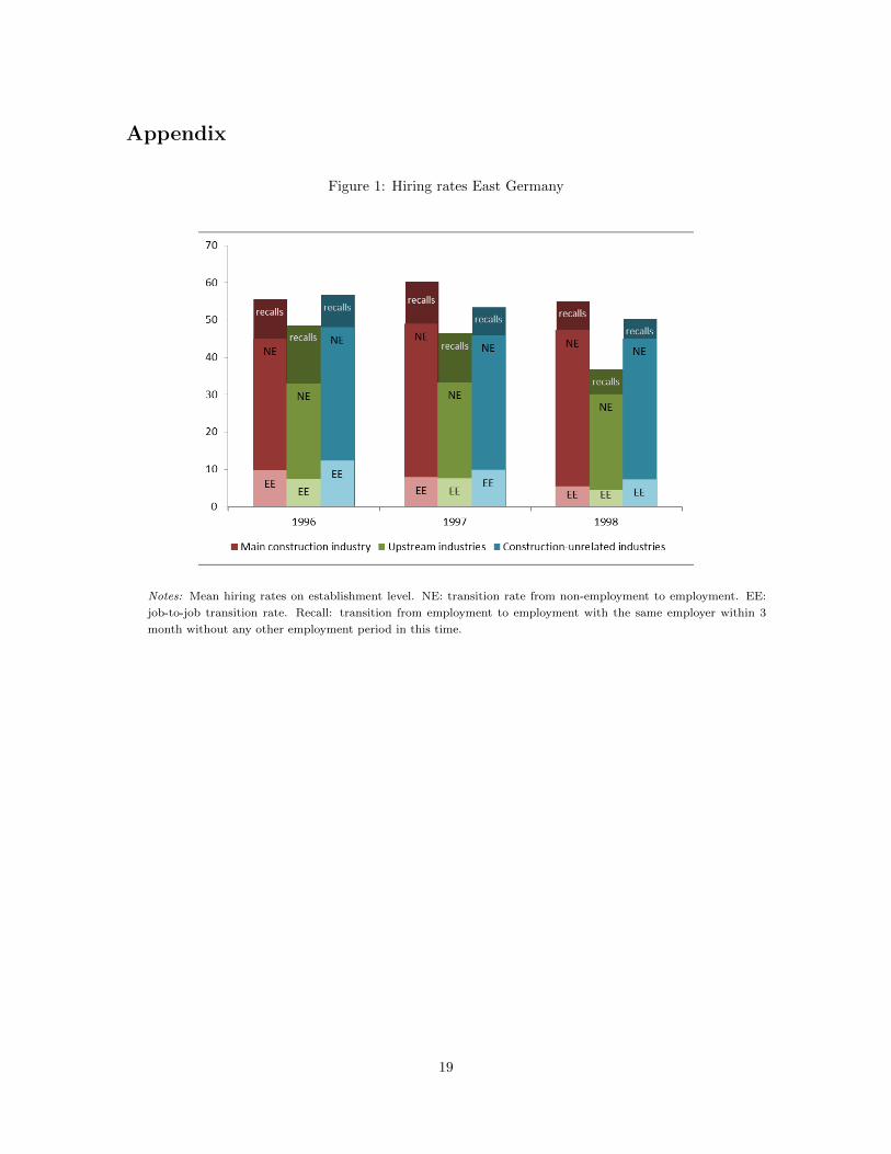
Figures 1 and 2 for East and West Germany, respectively. While hiring rates in the construction firms

in East Germany are higher than in West Germany, the evolution of hiring rates in construction in

East and West Germany are similar for the time period under investigation: From 1996 to 1997, one

can observe a relatively strong increase of these hiring rates. In the following year, hiring rates decline,

virtually undoing the preceding increase. By contrast, the hiring rates in both control industries in

East Germany feature a steady decline from 1996 to 1998. In West Germany, the hiring rates increase

monotonously in the construction-unrelated industries, while in the upstream industries they slightly

rise in 1997 and decline relatively strongly in 1998.

Looking at the hiring sources, it becomes evident that the increase of the hiring rate in the East

German construction industry in 1997 is due to a rise in hirings from non-employment, especially

recalls, which undoes the fall in hirings from employment. The decline in the following year is due to

both hiring transitions falling. For West Germany, a similar pattern can be observed. Here, hirings

from employment are virtually unchanged over time, i.e. hirings from non-employment, and especially

recalls, drive the evolution of overall hirings.

11

The separation rate (Figure 3) behaves very similarly to the hiring rate in East Germany. In

particular, one can observe an increase in 1997 and a decline in 1998, which brings the separation rate

virtually back to its 1996 level. This evolution is again driven by the transitions between employment

and non-employment as well as recalls. The separation rate in the West German construction industry

is also very similar to the one of the hiring rate. The separation rates in the West German control

industries, by contrast, display a decline (upstream industries) and a slight increase in 1997 and 1998

relative to 1996 (construction-unrelated). Table 2 shows the descriptives for our sample used in the

subsequent analysis.

5.2 Econometric evidence

In the following, we present the results from the difference-in-differences estimation explained in

Section 4. We do so for the overall levels of hirings and separations, for the underlying hirings flow

rates (hirings from another job, and hirings from non-employment), and for the underlying separation

flows (separations to another job, and separations to non-employment). Furthermore, we conduct

separate estimations for East and West Germany, as well as for the year 1997 and 1998 (both compared

to the year 1996).

The results for hirings and separations are displayed in Table 3.9 For East German hirings including

recalls, one can observe a positive effect for the construction industry compared to the construction-

unrelated control industry in 1997, but no effect compared to the upstream control industry. This

gives some indication for a positive effect, which however is not robust. For the year 1998, by contrast,

a clear positive effect becomes apparent. Without recalls, a positive effect emerges for the unrelated

control industries, but no effect for both years for the upstream control industries. Taken together,

this yields a positive effect for hirings in the main construction sector in 1998 only.

For separations in East Germany (lower panel of Table 3), the results for both control industries

in 1997 and 1998 indicate an unambiguously positive effect for hirings with recalls; for hirings without

recalls, the effect is insignificant when comparing the main construction sector to the upstream control

industries, while the effect using the unrelated control industries is still positively significant, but

smaller than for separations without recalls.

Taken together, these results imply a significant impact of between 3 and 7.6 percentage points

for hirings in East Germany for the year 1998, which corresponds to between 5 and 14 percent of

the overall hiring rate (about 55 percent in 1996), i.e. the effect is relatively large. This effect seems

to be mostly due to an increase in recalls in the main construction industry relative to the control

9The results tables generally only feature the marginal effects of the coefficient of the difference-in-differences

operator, i.e. λ3 in equation 4. For the calculation method see Section 4. A full set of coefficients for the estimation of

the hiring rate is contained in Table 4.

12

industries since it becomes smaller or insignificant if recalls are excluded. For separations, a similar

feature emerges. The effect lies between 5.2 and 6.6 percentage points including recalls, which equals

an increase between 9 and 11 percent of the overall separation rate, and virtually disappears for

separations without recalls.

For West Germany, no causal effect of the minimum wage introduction on hirings can be established

(upper panel of Table 3), as the comparison with the two control groups yields effects which are of

opposite sign (positive for the upstream industries, negative for the construction-unrelated industries),

which are partly insignificant. The picture for separations is similar in that the results for the two

control groups are opposite in sign (for separations including recalls) or insignificant (for separations

excluding recalls). This means that overall, we are not able to identify a clear effect of the minimum

wage neither for the hiring rate nor for the separation rate in the West German construction sector.

In the second step of the causal analysis, we examine the effect of the minimum wage introduction

on hirings in more detail, distinguishing between the two sources of hirings, i.e. hirings from em-

ployment (job-to-job transitions leading to hirings) and hirings from non-employment (hirings from

unemployment and non-participation). For East Germany, hirings out of employment are unaffected

by the minimum wage introduction in both 1997 and 1998 (Table 5). For hirings from non-employment

including recalls, we observe a significantly positive effect of between 1.6 and 9 percent. The latter

effect disappears or becomes smaller when recalls are excluded. This implies that the positive effect

on hirings can at least to some extent be explained by an increase in the hiring of workers which have

been employed by the same firm before, i.e. recalls.

Looking at the different hiring flows in West Germany, it becomes apparent that the minimum wage

introduction has no significant effect on job-to-job hirings (Table 5). In particular, the coefficients

of interest are mostly insignificant for job-to-job hirings. As for hirings from non-employment, the

upstream control industries yield insignificant results for the year 1997, and the two control groups

display opposite signs for the year 1998 which does not give a clear indication of a minimum wage

effect.

Finally, we scrutinize the effect of the minimum wage introduction on separations leading to a

new job match (job-to-job separations) and separations to non-employment separately. For East

Germany, the regression results show that separations to another job in 1997 were unaffected by the

introduction of the minimum wage (upper panel of Table 6). For the year 1998, however, a robust

negative effect on job-to-job separations becomes apparent. For separations into non-employment,

relatively large effects can be observed in East Germany. The minimum wage increased the rates by

5.2 to 8.3 percentage points which corresponds to an increase of between 10.7 and 17 percent of the

employment to non-employment rate. However, compared to this result, the effects on the transition

13

rate without recalls become smaller or even insignificant.

As for separations leading to another job, the coefficients for both years and both control industries

are insignificant. It thus becomes apparent that separations leading to another job are not affected

by the minimum wage introduction in West Germany (Table 6). Regarding West German separations

to non-employment (including recalls), the coefficients for the construction sector compared to the

upstream industries are positive and significant, but the coefficients for the construction-unrelated

control groups are negative and insignificant; excluding recalls, the results for both control groups are

insignificant.

Summarising, it becomes apparent that the introduction of minimum wages had effects in East

Germany: Both hirings and separations were positively affected, which seems to be due to an increase

in recalls, i.e. temporary transitions from employment to non-employment followed by transitions

from non-employment back to the same firm. Furthermore, we find some evidence that job-to-job

transitions fell after the introduction of minimum wages in East Germany. By contrast, we do not

find any (clear) evidence that the minimum wage introduction in West Germany had an effect on

either overall hirings and separations or on their underlying flows. Note that, with the exception of

separations in East Germany, these results are robust to the placebo-testing of the control groups

(see Section 4.4). The interpretation and the implications of these findings are discussed in the next

section.

6 Summary and Conclusions

In this paper, we analyse the effects of the introduction of minimum wages on labour market flows

in the German main construction industry in 1997. In particular, we examine overall hirings and

separations, as well as job-to-job transitions and the flows between employment and non-employment

at the establishment level. The fact that minimum wages in Germany are sector-specific allows us to

use comparable industries as control groups within a difference-in-differences framework and thus to

identify a truly causal effect.

Our analysis shows that the introduction of minimum wages had significant and quantitatively

important effects in East Germany. In particular, overall hirings and separations were both positively

affected. This seems to be mainly due to an increase in recalls, which we define as transitions from

employment to non-employment followed by transitions from non-employment back to the same firm

within a three-month period. One interpretation of this finding is that, after the introduction of

minimum wages, firms resort more often to temporarily laying off workers in order to save on increased

wage costs.

A second minimum wage effect we identify for East Germany is a reduction of job-to-job transi-

14

tions. This effect can be explained by the evolution of the wage distribution in East Germany, which

became more compressed after the introduction of minimum wages in 1997. A more compressed wage

distribution reduces the incentives of employed workers to engage in on-the-job search, as the expected

gains from searching while employed are reduced, which in turn lowers job-to-job transitions (van den

Berg and Ridder, 1998).

In contrast to the results for East Germany, we do not find clear evidence that the minimum wage

introduction had an effect on labour market dynamics in West Germany. This result is not surprising

given that the minimum wage was binding for relatively few workers in West Germany when it was

introduced.

Our results, especially the ones for East Germany where minimum wages in the main construction

sector are binding, thus add interesting insights into the effects of minimum wages. First, our results

suggest that, by compressing the wage structure, minimum wages reduce job-to-job transitions.

Second, we show that the introduction of minimum wages may well increase labour market flows.

This stands in contrast to the previous literature which has found a dampening effect of minimum

wages on accessions and separations for Canada (Brochu and Green, 2011), Portugal (Portugal and

Cardoso, 2006) and the US (Dube et al., 2011). It seems likely that our result is due to our focus on

short-run effects, where transitory dynamics, rather than equilibrium effects, dominate. In addition,

the result may be partly due to the specificities of the main construction industry, which is generally

characterised by high turnover rates and a high prevalence of recalls.

Third, our results complement and add to the literature on minimum wages in Germany. In

particular, we qualify the result by Konig and Moller (2009) who found relatively small effects of the

minimum wage in the German main construction industry on employment security, especially in East

Germany. The much larger effects uncovered by our analysis are likely to be due to the relatively long

time period (January 1 to August 31) that is used for identifying labour market flows both in the year

before the minimum wage introduction (1997) as well as for the two years after the minimum wage

introduction. Apparently, our analysis is thus able to capture important effects which take place early

in the calendar year.

Finally, a word of caution regarding further interpretation of the results is in order. While the

industry-specificity of minimum wages allows us to identify a causal effect by using industries not

affected by minimum wages as control groups for the main construction industry, the downside of

our approach is that the results cannot easily be generalised. In particular, our results apply to the

main construction industry only; whether other industries would experience similar effects upon the

introduction of minimum wages is thus not clear at all. This is all the more important because the

main construction industry displays several peculiarities, in particular a large number of foreign, posted

15

workers before the introduction of minimum wages. Given that minimum wages were introduced in

this sector for mainly protectionist reasons, this group of workers may have experienced negative

labour market effects. Unfortunately, there is no data to identify a causal effect of minimum wages on

this group. For these reasons, our results should not be generalised to the effects of minimum wages

in other sectors, or to the effects of a generally binding minimum wage.

16

References

Apel, Helmut, Ronald Bachmann, Stefan Bender, Philipp vom Berge, Michael Fertig,

Marion Konig, Hanna Krger, Joachim Moller, Alfredo Paloyo, Sandra Schaffner, Mar-

cus Tamm, Matthias Umkehrer, and Stefanie Wolter, “Arbeitsmarktwirkungen der Mindest-

lohneinfuhrung im Bauhauptgewerbe,” Zeitschrift fur Arbeitsmarktforschung, 2012, (forthcoming).

Bachmann, R., Th.K. Bauer, J. Kluve, S. Schaffner, and Ch.M. Schmidt, “Mindestlohne in

Deutschland Beschaftigungswirkungen und fiskalische Effekte,” RWI Materialien 43, Essen 2008.

Bachmann, Ronald, Thomas Bauer, and Hanna Kroeger, “Minimum Wages as a Barrier to

Entry: Evidence from Germany,” IZA Discussion Papers 6484, Institute for the Study of Labor

(IZA) April 2012.

Bauer, Th. K., J. Kluve, S. Schaffner, and Ch. M. Schmidt, “Fiscal Effects of Minimum

Wages: An Analysis for Germany,” German Economic Review, 2009, 10 (2), 224–242.

Brochu, Pierre and David A. Green, “The impact of minimum wages on quit, layoff and hiring

rates,” IFS Working Papers, Institute for Fiscal Studies April 2011.

Burgess, Simon, Julia Lane, and David Stevens, “Churning dynamics: an analysis of hires and

separations at the employer level,” Labour Economics, 2001, 8 (1), 1–14.

Card, David and Alan B Krueger, “Minimum Wages and Employment: A Case Study of the

Fast-Food Industry in New Jersey and Pennsylvania,” American Economic Review, September 1994,

84 (4), 772–93.

Dorner, Matthias, Jorg Heining, Peter Jacobebbinghaus, and Stefan Seth, “Sample of

Integrated Labour Market Biographies (SIAB) 1975-2008,” FDZ-Datenreport 01/10, Nuremberg

2010.

Dube, Andrajit, T. William Lester, and Michael Reich, “Minimum Wage Effects Across State

Borders: Estimates Using Contiguous Counties,” Review of Economics and Statistics, November

2010, 92 (4), 945–64.

Dube, Arindrajit, T. William Lester, and Michael Reich, “Do frictions matter in the labor

market? Accessions, separations and minimum wage effects,” IZA Discussion Papers, Institute for

the Study of Labor (IZA) June 2011.

Frings, Hanna, “The employment effect of industry-specific, collectively-bargained minimum wages,”

Ruhr Economic Papers 348, Rheinisch-Westfalisches Institut fur Wirtschaftsforschung, Ruhr-

Universitat Bochum, Universitat Dortmund, Universitat Duisburg-Essen 2012.

17

Frondel, Manuel and Colin Vance, “On Interaction Effects: The Case of Heckit and Two-Part

Models,” Ruhr Economic Papers 309, Rheinisch-Westfalisches Institut fur Wirtschaftsforschung,

Ruhr-Universitat Bochum, Universitat Dortmund, Universitat Duisburg-Essen January 2012.

Hethey, T. and J. Schmieder, “Using Worker Flows in the Analysis of Establishment Turnover

Evidence from German Administrative Data,” FDZ-Methodenreport 06/2010, Nuremberg 2010.

Konig, Marion and Joachim Moller, “Impacts of minimum wages: a microdata analysis for the

German construction sector,” International Journal of Manpower, November 2009, 30 (7), 716–741.

Lechner, Michael, “The Estimation of Causal Effects by Difference-in-Difference Methods,” Uni-

versity of St. Gallen Department of Economics working paper series 2010 2010-28, Department of

Economics, University of St. Gallen September 2010.

Mortensen, Dale T and Christopher A Pissarides, “Job Creation and Job Destruction in the

Theory of Unemployment,” Review of Economic Studies, July 1994, 61 (3), 397–415.

Muller, K.-U. and V. Steiner, “Would a Legal Minimum Wage Reduce Poverty? - A Microsimu-

lation Study for Germany,” DIW Discussion Papers 791, Berlin 2008.

Muller, Kai-Uwe, “Employment Effects of a Sectoral Minimum Wage in Germany,” DIW Discussion

Papers 1061, Berlin 2010.

Neumark, David and William L. Wascher, Minimum Wages, The MIT Press, 2008.

Portugal, Pedro and Ana Rute Cardoso, “Disentangling the minimum wage puzzle: An analysis

of worker accessions and separations,” Journal of the European Economic Association, 09 2006, 4

(5), 988–1013.

Puhani, Patrick A., “The Treatment Effect, the Cross Difference, and the Interaction Term in

Nonlinear Difference-in-Differences Models,” Economics Letters, 2012, 115, 85–87.

Rattenhuber, Pia, “Building the Minimum Wage. Germanys First Sectoral Minimum Wage and its

Impact on Wages in the Construction Industry,” DIW Discussion Papers 1111, Berlin 2011.

van den Berg, Gerard J. and Geert Ridder, “An Empirical Equilibrium Search Model of the

Labor Market,” Econometrica, September 1998, 66 (5), 1183–1222.

18

Appendix

Figure 1: Hiring rates East Germany

Notes: Mean hiring rates on establishment level. NE: transition rate from non-employment to employment. EE:

job-to-job transition rate. Recall: transition from employment to employment with the same employer within 3

month without any other employment period in this time.

19

Figure 2: Hiring rates West Germany

Notes: Mean hiring rates on establishment level. NE: transition rate from non-employment to employment. EE:

job-to-job transition rate. Recall: transition from employment to employment with the same employer within 3

month without any other employment period in this time.

20

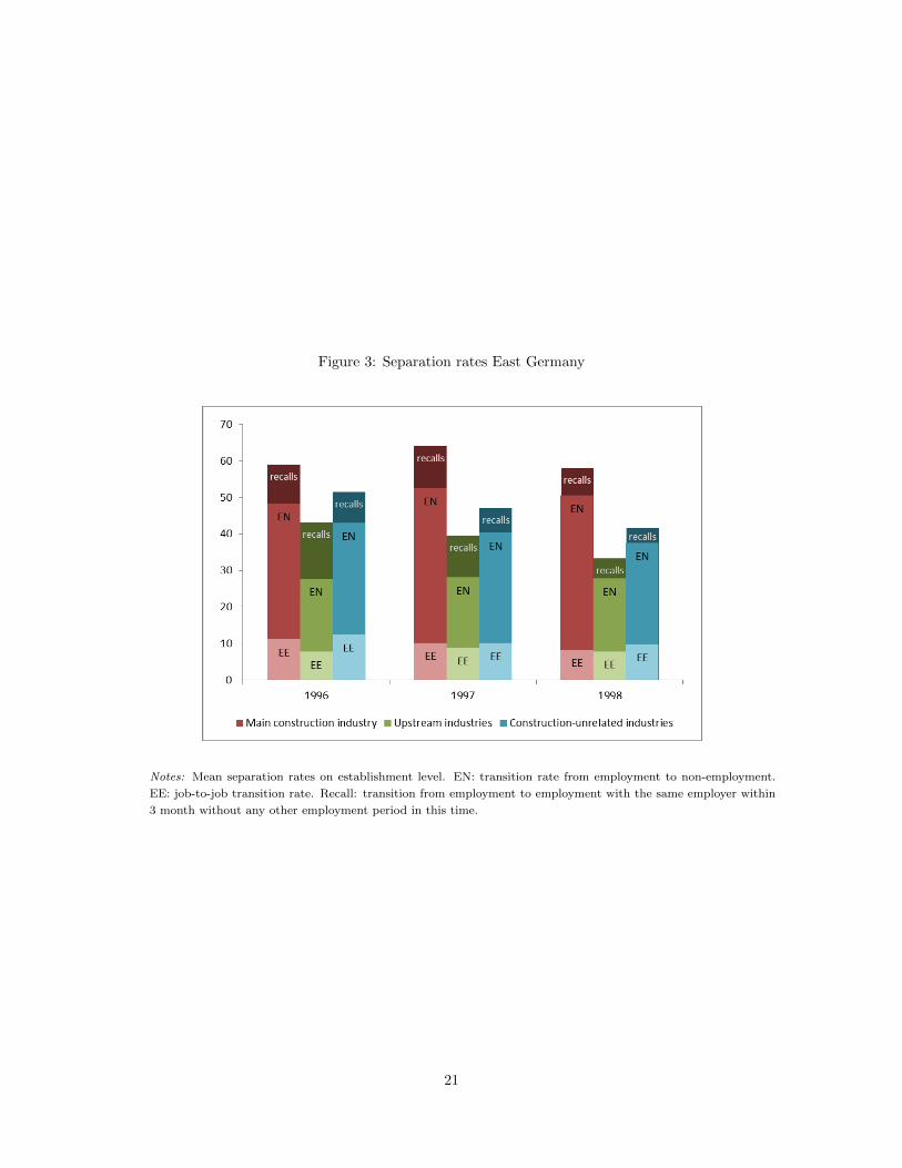
Figure 3: Separation rates East Germany

Notes: Mean separation rates on establishment level. EN: transition rate from employment to non-employment.

EE: job-to-job transition rate. Recall: transition from employment to employment with the same employer within

3 month without any other employment period in this time.

21

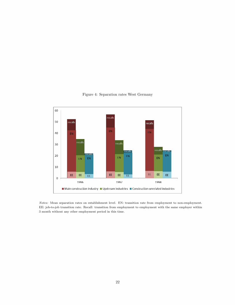
Figure 4: Separation rates West Germany

Notes: Mean separation rates on establishment level. EN: transition rate from employment to non-employment.

EE: job-to-job transition rate. Recall: transition from employment to employment with the same employer within

3 month without any other employment period in this time.

22

Table 1: Definition of Treatment and Control Groups

Treatment Group Industry Code Sector

Main Construction 590 General civil engineering activities

591 Building construction and civil engineering

592 Civil and underground

593 Construction of chimneys and furnaces

594 Plasterers and foundry dressing shops

600 Carpentry and timber construction

614 Floor tilers and paviors

Control Groups Industry Code Sector

(ii) West 431 Processing of paper and paperboard

(ii) East 651 Carriage of goods by motor vehicles

(iv) West and East 146 Manufacture of sand-lime brick, concrete and mortar

Notes:Industry codes according to the Classification of Economic Activities of the German Federal Employment Agency1973 (Wirtschaftszweige nach BA-Klassifikation 1973), (WZ 73).For information on the selection procedure of the control groups please see text.

23

Table 2: Sample descriptives, averages for 1996-1998

Sample descriptives East Germany West Germany

Number of firms

Main construction industry 85,767 230,127

Upstream industries 3,692 9,730

Construction-unrelated industries 24,375 2,404

Number of employees

Main construction industry 1,739,001 888,417

Upstream industries 127,458 46,515

Construction-unrelated industries 48,523 103,248

Firm characteristics (averages)

Number of employees

Main construction industry 10.36 7.56

Upstream industries 12.60 13.10

Construction-unrelated industries 4.24 20.18

Worker age

Main construction industry

Upstream industries

Construction-unrelated industries

Wage level

Main construction industry 9.01 12.18

Upstream industries 9.93 14.07

Construction-unrelated industries 7.38 12.49

Number of employees Main construction industry 26.67 13.18

below MW at introduction Upstream industries 18.11 3.22

(share in %) Construction-unrelated industries 63.04 8.39

24

Table 3: Difference-in-differences results transitions

upstream unrelated

Hir

ings

with recalls 1997 0.033 0.040 **

Eas

t

1998 0.076 ** 0.030 **

without recalls 1997 0.018 0.032 **

1998 0.027 0.026 **

with recalls 1997 0.033 ** -0.051

Wes

t

1998 0.085 ** -0.116 **

without recalls 1997 0.006 -0.056 *

1998 0.045 ** -0.101 **

Sep

ara

tion

s

with recalls 1997 0.052 ** 0.064 **

Eas

t1998 0.066 ** 0.057 **

without recalls 1997 0.018 0.047 **

1998 0.002 0.045 **

with recalls 1997 0.022 * -0.010

Wes

t

1998 0.051 ** -0.045

without recalls 1997 -0.007 -0.015

1998 -0.006 -0.034

Notes: Marginal effects, ∗ significance at the 10% level, ∗∗ significance at the 5% level. The standard errors arecalculated based on the delta method.For the description of the additional covariates and the estimation method see text.

25

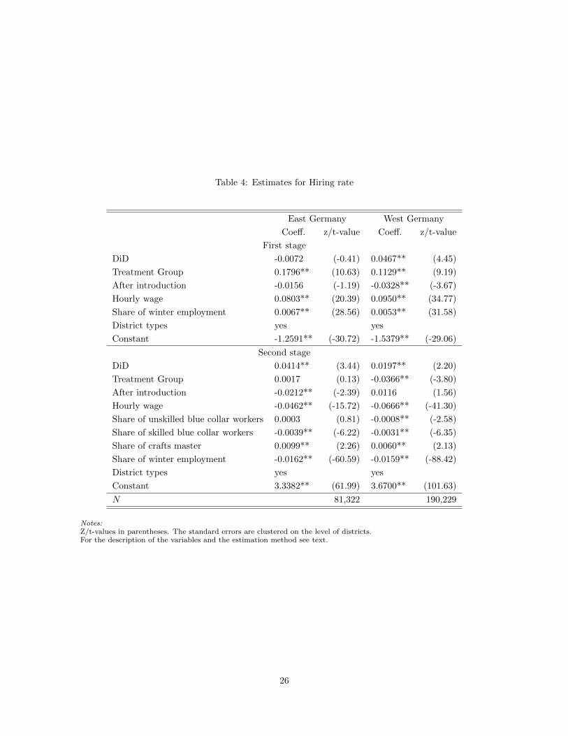
Table 4: Estimates for Hiring rate

East Germany West Germany

Coeff. z/t-value Coeff. z/t-value

First stage

DiD -0.0072 (-0.41) 0.0467** (4.45)

Treatment Group 0.1796** (10.63) 0.1129** (9.19)

After introduction -0.0156 (-1.19) -0.0328** (-3.67)

Hourly wage 0.0803** (20.39) 0.0950** (34.77)

Share of winter employment 0.0067** (28.56) 0.0053** (31.58)

District types yes yes

Constant -1.2591** (-30.72) -1.5379** (-29.06)

Second stage

DiD 0.0414** (3.44) 0.0197** (2.20)

Treatment Group 0.0017 (0.13) -0.0366** (-3.80)

After introduction -0.0212** (-2.39) 0.0116 (1.56)

Hourly wage -0.0462** (-15.72) -0.0666** (-41.30)

Share of unskilled blue collar workers 0.0003 (0.81) -0.0008** (-2.58)

Share of skilled blue collar workers -0.0039** (-6.22) -0.0031** (-6.35)

Share of crafts master 0.0099** (2.26) 0.0060** (2.13)

Share of winter employment -0.0162** (-60.59) -0.0159** (-88.42)

District types yes yes

Constant 3.3382** (61.99) 3.6700** (101.63)

N 81,322 190,229

Notes:Z/t-values in parentheses. The standard errors are clustered on the level of districts.For the description of the variables and the estimation method see text.

26

Table 5: Difference-in-differences detailed hiring rates

upstream unrelated

Job

-to-

job 1997 -0.016 -0.002

Eas

t

1998 -0.005 -0.003

1997 0.003 -0.002

Wes

t

1998 -0.002 -0.020 **

un

emp

loym

ent/

non

-par

tici

pat

ion

with recalls 1997 0.035 0.037 **

Eas

t

1998 0.090 ** 0.016 *

without recalls 1997 0.018 0.029 **

1998 0.043 * 0.012

with recalls 1997 0.020 -0.063 *

Wes

t

1998 0.084 ** -0.096 **

without recalls 1997 -0.005 -0.066 **

1998 0.044 ** -0.081 **

Notes: Marginal effects, ∗ significance at the 10% level, ∗∗ significance at the 5% level. The standard errors are calculated based on the delta

method.

For the description of the additional covariates and the estimation method see text.

Table 6: Difference-in-differences detailed separations

upstream unrelated

Job

-to-

job 1997 -0.016 0.006

Eas

t

1998 -0.022 ** -0.010 **

1997 0.003 -0.003

Wes

t

1998 -0.004 -0.014

un

emp

loym

ent

non

-par

tici

pat

ion

with recalls 1997 0.062 ** 0.052 **

Eas

t

1998 0.083 ** 0.060 **

without recalls 1997 0.027 0.036 **

1998 0.011 0.047 **

with recalls 1997 0.023 ** -0.017

Wes

t

1998 0.068 ** -0.032

without recalls 1997 -0.008 -0.018

1998 0.011 -0.023

Notes: Marginal effects, ∗ significance at the 10% level, ∗∗ significance at the 5% level. The standard errors are calculated based on the delta

method.

For the description of the additional covariates and the estimation method see text.

27

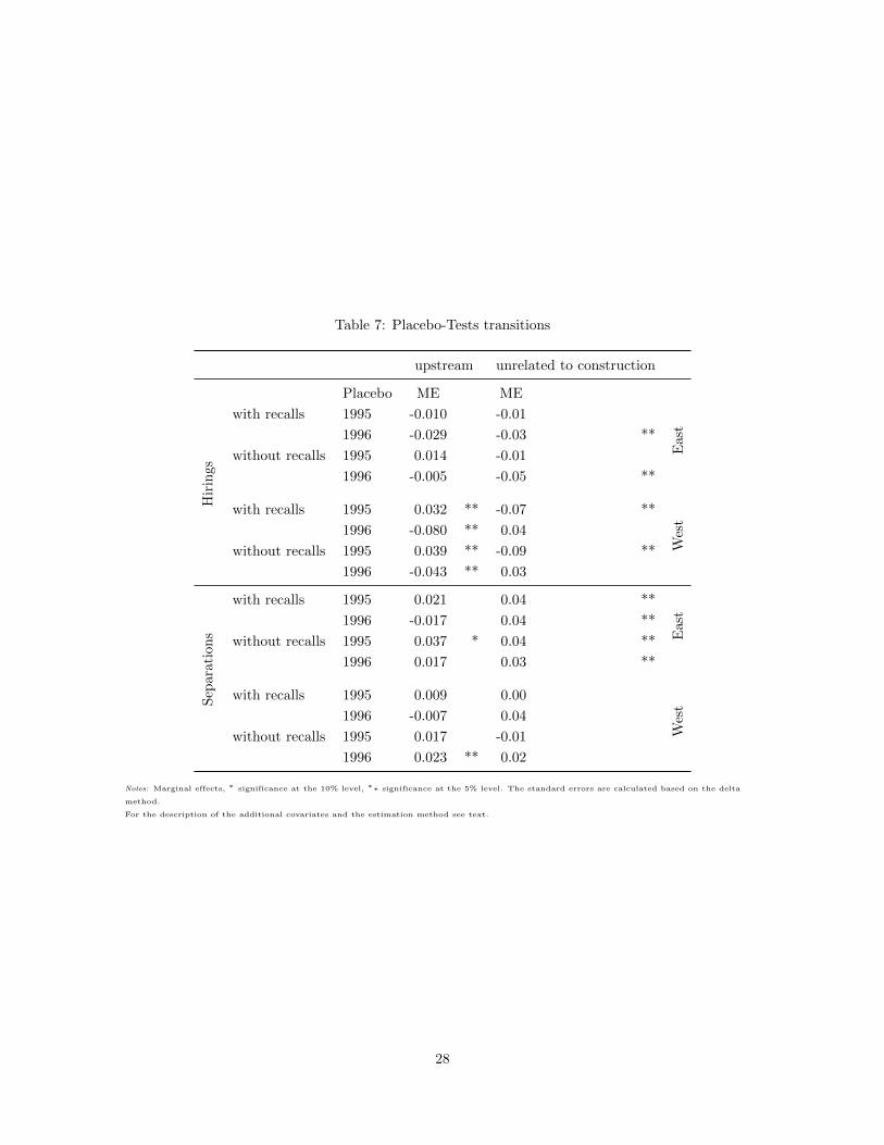
Table 7: Placebo-Tests transitions

upstream unrelated to construction

Placebo ME ME

Hir

ings

with recalls 1995 -0.010 -0.01

Eas

t

1996 -0.029 -0.03 **

without recalls 1995 0.014 -0.01

1996 -0.005 -0.05 **

with recalls 1995 0.032 ** -0.07 **

Wes

t

1996 -0.080 ** 0.04

without recalls 1995 0.039 ** -0.09 **

1996 -0.043 ** 0.03

Sep

arati

on

s

with recalls 1995 0.021 0.04 **

Eas

t

1996 -0.017 0.04 **

without recalls 1995 0.037 * 0.04 **

1996 0.017 0.03 **

with recalls 1995 0.009 0.00W

est

1996 -0.007 0.04

without recalls 1995 0.017 -0.01

1996 0.023 ** 0.02

Notes: Marginal effects, ∗ significance at the 10% level, ∗∗ significance at the 5% level. The standard errors are calculated based on the delta

method.

For the description of the additional covariates and the estimation method see text.

28

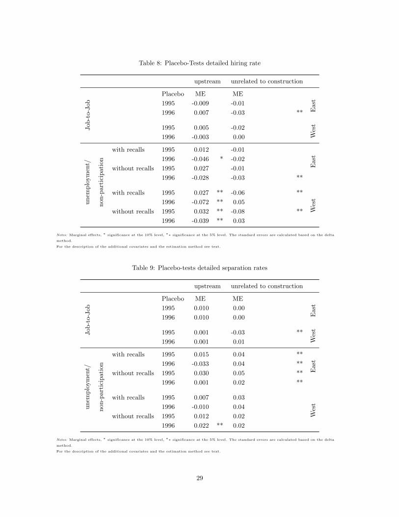
Table 8: Placebo-Tests detailed hiring rate

upstream unrelated to construction

Placebo ME MEJob

-to-

Job 1995 -0.009 -0.01

Eas

t

1996 0.007 -0.03 **

1995 0.005 -0.02

Wes

t

1996 -0.003 0.00

un

emp

loym

ent/

non

-par

tici

pati

on

with recalls 1995 0.012 -0.01

East1996 -0.046 * -0.02

without recalls 1995 0.027 -0.01

1996 -0.028 -0.03 **

with recalls 1995 0.027 ** -0.06 **

Wes

t1996 -0.072 ** 0.05

without recalls 1995 0.032 ** -0.08 **

1996 -0.039 ** 0.03

Notes: Marginal effects, ∗ significance at the 10% level, ∗∗ significance at the 5% level. The standard errors are calculated based on the delta

method.

For the description of the additional covariates and the estimation method see text.

Table 9: Placebo-tests detailed separation rates

upstream unrelated to construction

Placebo ME ME

Job

-to-

Job 1995 0.010 0.00

Eas

t1996 0.010 0.00

1995 0.001 -0.03 **

Wes

t

1996 0.001 0.01

un

emp

loym

ent/

non

-par

tici

pat

ion

with recalls 1995 0.015 0.04 **

Eas

t

1996 -0.033 0.04 **

without recalls 1995 0.030 0.05 **

1996 0.001 0.02 **

with recalls 1995 0.007 0.03

Wes

t1996 -0.010 0.04

without recalls 1995 0.012 0.02

1996 0.022 ** 0.02

Notes: Marginal effects, ∗ significance at the 10% level, ∗∗ significance at the 5% level. The standard errors are calculated based on the delta

method.

For the description of the additional covariates and the estimation method see text.

29