Loop Shaping from Bode-Nyquist to Glover-McFarlane

Loop Shapingfrom Bode-Nyquist to Glover-McFarlane

K. J. Åström

Department of Automatic Control, Lund University

K. J. Åström Loop Shaping from Bode-Nyquist to Glover-McFarl ane

Congratulations Keith

Visionary leadership in CambridgeGreat fundamental researchUseful applications with strong industrial impactSuperb studentsExcellent service to the UniversityGenuinely nice person with a glimpse in your eye

Your monumental model reduction paper

Your tour de force on H∞ theory and design methods

H∞ loop shaping (elegant theory, lots of applications)

Congratulations to scholar and a gentleman!


Outline

1 Introduction2 Bode’s Ideal Cut-off Characteristic3 Loop Shaping4 H∞ Loop Shaping5 Summary


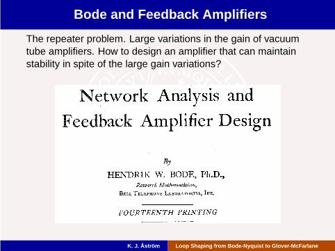
Bode and Feedback Amplifiers

The repeater problem. Large variations in the gain of vacuumtube amplifiers. How to design an amplifier that can maintainstability in spite of the large gain variations?


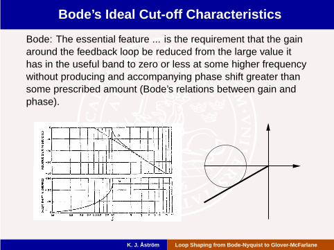
Bode’s Ideal Cut-off Characteristics

Bode: The essential feature ... is the requirement that the gainaround the feedback loop be reduced from the large value ithas in the useful band to zero or less at some higher frequencywithout producing and accompanying phase shift greater thansome prescribed amount (Bode’s relations between gain andphase).


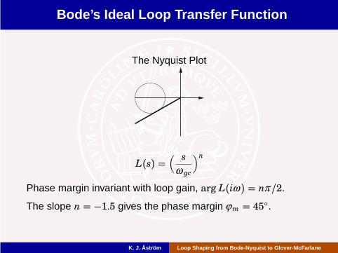
Bode’s Ideal Loop Transfer Function

The Nyquist Plot

L(s) =( s

ω�c

)n

Phase margin invariant with loop gain, arg L(iω ) = nπ /2.The slope n = −1.5 gives the phase margin ϕm = 45○.


Trade-offs

Bode (page 454): If it were not for the phase restriction it wouldbe desirable to on engineering grounds to reduce gain veryrapidly. The more rapidly the gain vanishes, for example, thenarrower we need to make the region in which active designattenuation is required to prevent singing.

L(s) = sn,n = −5/3 (ϕm = 30○),−4/3 (ϕm = 60○),−1 (ϕm = 90○)

10−1

100

101

10−1

100

101

Frequency ω

pL(iω)p


An Example

Consider a process with the transfer function

P(s) = k

s(s+ 1)

Assume that we would like to have a closed loop system thathas a phase margin ϕm = 45○ for large variations of the gain.Bode’s ideal loop transfer function is

L(s) = 1

s√s

Since L = PC the controller transfer function becomes (k = 1)

C(s) = L(s)P(s) =

s+ 1√s=√s+ 1√

s


Step Responses

P(s) = k

s(s+ 1) , C(s) =√s+ 1√

s, k = 1, 5, 25

0 1 2 3 4 5 6 7 8 9 100

0.5

1

1.5

Time t

y

Time scales as k2/3 (slope is n = −3/2)


Outline



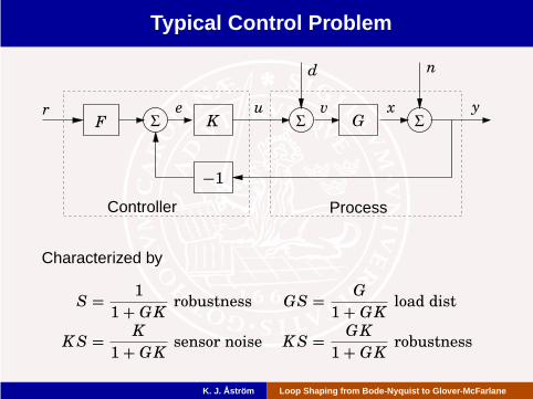
Typical Control Problem

F K G

Controller Process

−1

Σ Σ Σr e u

d

x

n

yv

Characterized by

S = 1

1+ GK robustness GS = G

1+ GK load dist

KS = K

1+ GK sensor noise KS = GK

1+ GK robustness


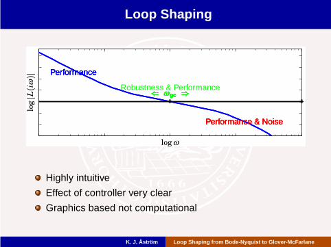
Loop Shaping

Z ω gc [Z ω gc [Z ω gc [Z ω gc [

Performance & NoisePerformance & NoisePerformance & NoisePerformance & Noise

PerformancePerformancePerformancePerformance

Robustness & Performance

logpL(iω)p

logω

Highly intuitive

Effect of controller very clear

Graphics based not computational


ASEA Experience of Loop Shaping

We had designed controllers by making simplified models,applying intuition and analyzing stability by solving thecharacteristic equation. (At that time, around 1950, solving thecharacteristic equation with a mechanical calculator was itselfan ordeal.) If the system was unstable we were at a loss, wedid not know how to modify the controller to make the systemstable. The Nyquist theorem was a revolution for us. Bydrawing the Nyquist curve we got a very effective way to designthe system because we know the frequency range which wascritical and we got a good feel for how the controller should bemodified to make the system stable. We could either add acompensator or we could use extra sensor.

Erik Persson Free translation from seminar in Lund.


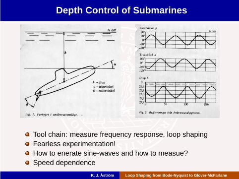
Depth Control of Submarines

Tool chain: measure frequency response, loop shapingFearless experimentation!How to enerate sine-waves and how to measue?Speed dependence


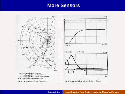
More Sensors

,


More Complicated Uncertainties - Horowitz QFT

Horowitz inherited Bode’s deep insight into feedbackBode [ Guillemin [ Truxal [ Horowitz

Extended Bode’s results to more general parameter variations

Quote from Horowitz IEEE CSM 4(1984) 22–23

It is amazing how many are unaware that the primary reasonfor feedback in control is uncertainty.

And why bother with listing all the states if only one one couldactually be measured and used for feedback? If indeed therewere several available, their importance in feedback was theirability to drastically reduce the effect of sensor noise, whichwas very transparent in and input-output frequency responseformulation and terribly obscure in the state-variable form. Forthese reasons, I stayed with the input-output description.


Outline



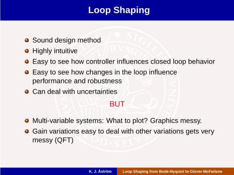
Loop Shaping

Sound design method

Highly intuitive

Easy to see how controller influences closed loop behavior

Easy to see how changes in the loop influenceperformance and robustness

Can deal with uncertainties

BUT

Multi-variable systems: What to plot? Graphics messy.

Gain variations easy to deal with other variations gets verymessy (QFT)


Glover and McFarlane Enter the Field

What to plot? - Singular values!How to characterize uncertainties? - Coprime factorization!How to specify requirements? - Frequency weights!How to compute? - H∞!479+652 citations!


A Flexible Drive

100

101

102

103

10−2

10−1

100

101

100

101

102

103

−720

−540

−360

−180

0

ω

pG(iω)p,pL(iω)|

argG(iω)

−1.5 −1 −0.5 0 0.5 1−1.5

−1

−0.5

0

0.5

ReL(iω )

ImL(iω)

G(s) = 5 (−s+ 40)(s+ 40)2(s2 + s+ 160)(s2 + 3s+ 1900) e

−0.1s

K (s) = 50

s(s+ 5)2


Transfer Function G(s), S(s)G(s)

10−1

100

101

102

10−1

100

101

ω

pG(iω)|pSG(iω)|

G(s) = 5 (−s+ 40)(s+ 40)2(s2 + s+ 160)(s2 + 3s+ 1900) e

−0.1s

K (s) = 50

s(s+ 5)2


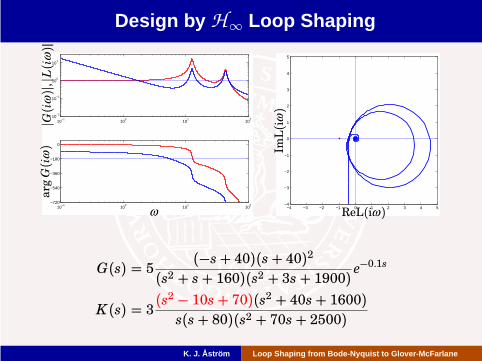
Design by H∞ Loop Shaping

10−1

100

101

102

10−2

10−1

100

101

10−1

100

101

102

−720

−540

−360

−180

0

ω

pG(iω)p,pL(iω)|

argG(i ω)

−4 −3 −2 −1 0 1 2 3 4 5−4

−3

−2

−1

0

1

2

3

4

5

ReL(iω )

ImL(iω)

G(s) = 5 (−s+ 40)(s+ 40)2(s2 + s+ 160)(s2 + 3s+ 1900) e

−0.1s

K (s) = 3(s2 − 10s+ 70)(s2 + 40s+ 1600)s(s+ 80)(s2 + 70s+ 2500)


Transfer Function S(s)G(s)

10−1

100

101

102

10−2

10−1

100

101

ω

pG(iω)p,pPS(iω)|

G(s) = 5 (−s+ 40)(s+ 40)2(s2 + s+ 160)(s2 + 3s+ 1900) e

−0.1s

K (s) = 3 (s2 − 10s+ 70)(s2 + 40s+ 1600)s(s+ 80)(s2 + 70s+ 2500)


Comparison 1

10−1

100

101

102

10−2

10−1

100

101

10−1

100

101

102

−720

−540

−360

−180

0

ω


Comparison 2

10−1

100

101

102

10−1

100

101

ω

pGS(iω)|


Outline



Summary

Retain the intuitive appeal of classical loop shaping

Specify load disturbance attenuation and noise injection byfrequency weights

Efficient numerical computations

Elegant mathematics

A really useful engineering design tool

The Beauty of H∞ loop shaping: Keep the SISO intuitionavoid acrobatics in Nyquist and Nichols plots and enjoy simpleways to deal with requirements and efficient computations.

A very effective design method!

Congratulations!


Loop Shaping from Bode-Nyquist to Glover-McFarlane

Documents

Transcript of Loop Shaping from Bode-Nyquist to Glover-McFarlane