Looking at data: distributions- Describing distributions with numbersIPS section 1.2

© 2006 W.H. Freeman and Company (authored by Brigitte Baldi, University of California-Irvine; adapted by Jim Brumbaugh-Smith, Manchester College)

Objectives

Describing distributions with numbers

Describe center of a set of data

Describe positions within a set of data

Represent quartiles graphically

Identify outliers mathematically

Describe amount of variation (or “spread”) in a set of data

Choose appropriate summary statistics

Describe effects of linear transformations

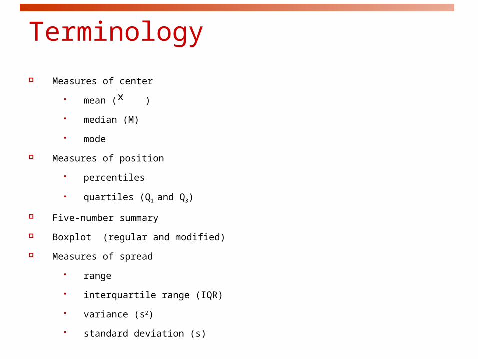
Terminology

Measures of center

mean ( )

median (M)

mode

Measures of position

percentiles

quartiles (Q1 and Q3)

Five-number summary

Boxplot (regular and modified)

Measures of spread

range

interquartile range (IQR)

variance (s2)

standard deviation (s)

x

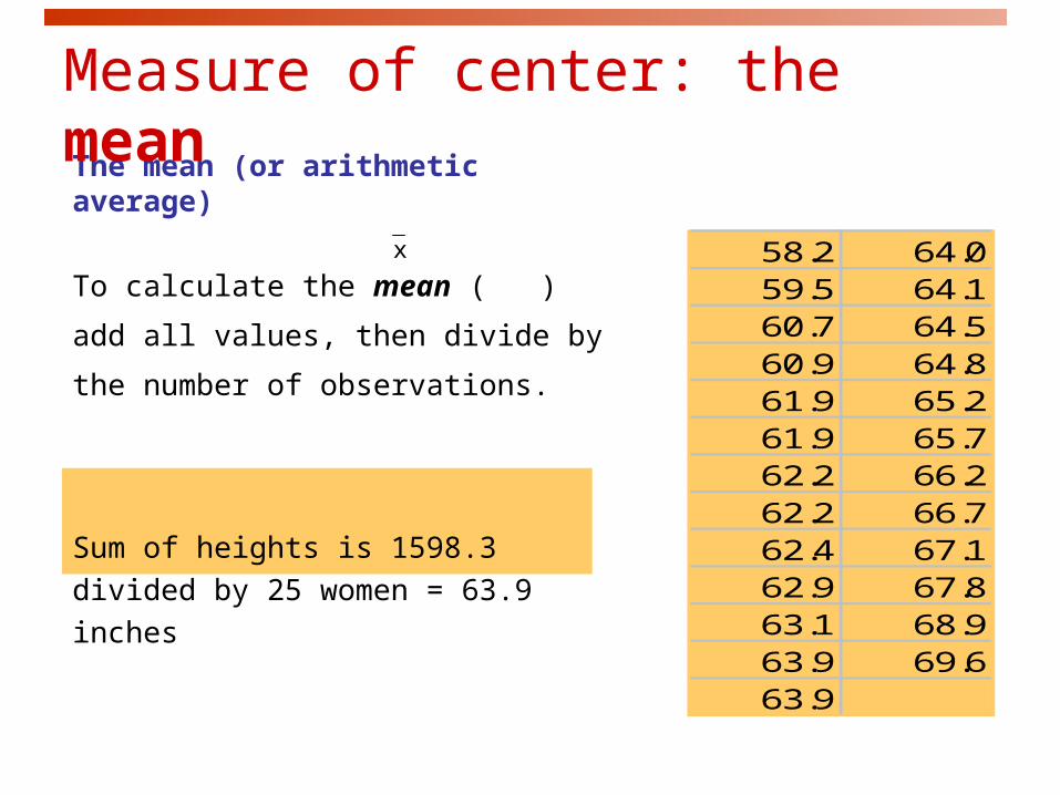
The mean (or arithmetic average)

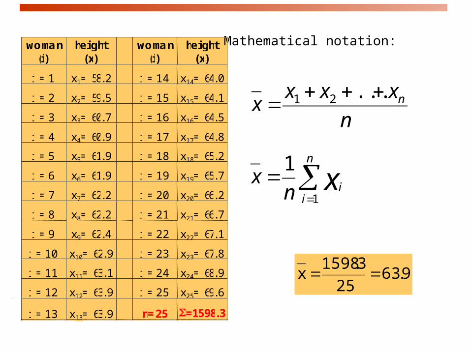
To calculate the mean ( ) add all

values, then divide by the number of

observations.

Sum of heights is 1598.3

divided by 25 women = 63.9 inches

58.2 64.059.5 64.160.7 64.560.9 64.861.9 65.261.9 65.762.2 66.262.2 66.762.4 67.162.9 67.863.1 68.963.9 69.663.9

Measure of center: the mean

x

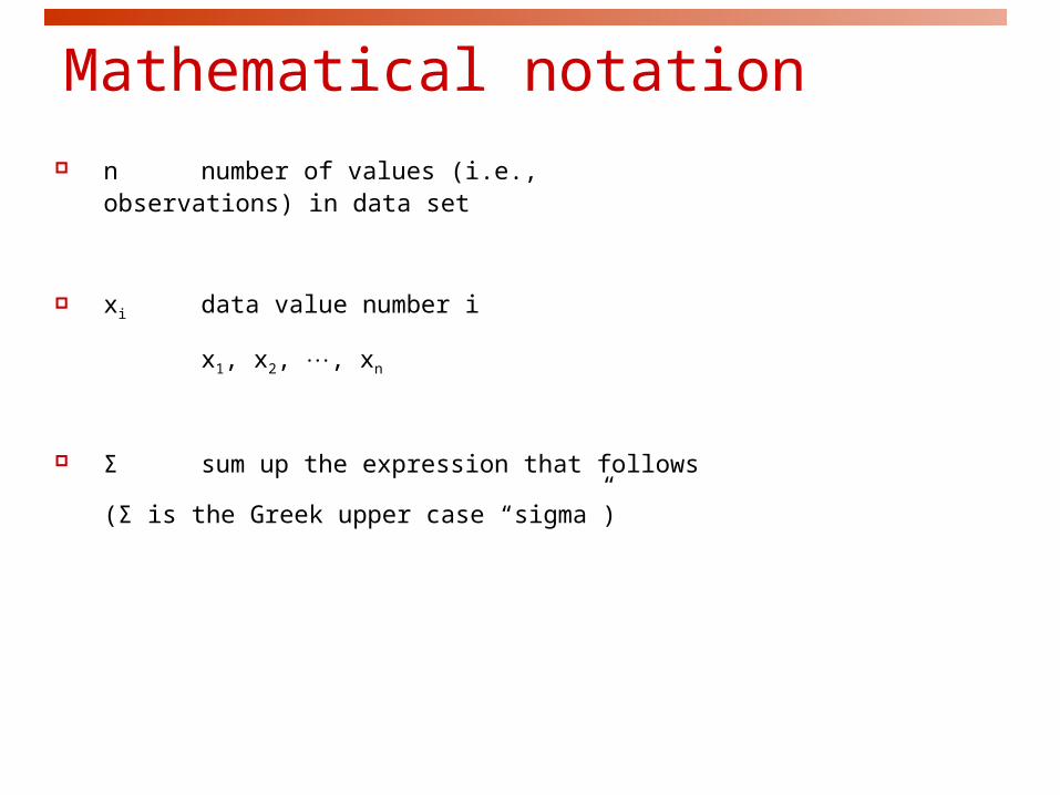
Mathematical notation n number of values (i.e., observations) in data

set

xi data value number i

x1, x2, , xn

Σ sum up the expression that follows

(Σ is the Greek upper case “sigma”)

9.6325

3.1598x

Mathematical notation:

n

iixn

x1

1

woman(i)

height(x)

woman(i)

height(x)

i = 1 x1= 58.2 i = 14 x14= 64.0

i = 2 x2= 59.5 i = 15 x15= 64.1

i = 3 x3= 60.7 i = 16 x16= 64.5

i = 4 x4= 60.9 i = 17 x17= 64.8

i = 5 x5= 61.9 i = 18 x18= 65.2

i = 6 x6= 61.9 i = 19 x19= 65.7

i = 7 x7= 62.2 i = 20 x20= 66.2

i = 8 x8= 62.2 i = 21 x21= 66.7

i = 9 x9= 62.4 i = 22 x22= 67.1

i = 10 x10= 62.9 i = 23 x23= 67.8

i = 11 x11= 63.1 i = 24 x24= 68.9

i = 12 x12= 63.9 i = 25 x25= 69.6

i = 13 x13= 63.9 n= 25 =1598.3

n

xxxx n

...21

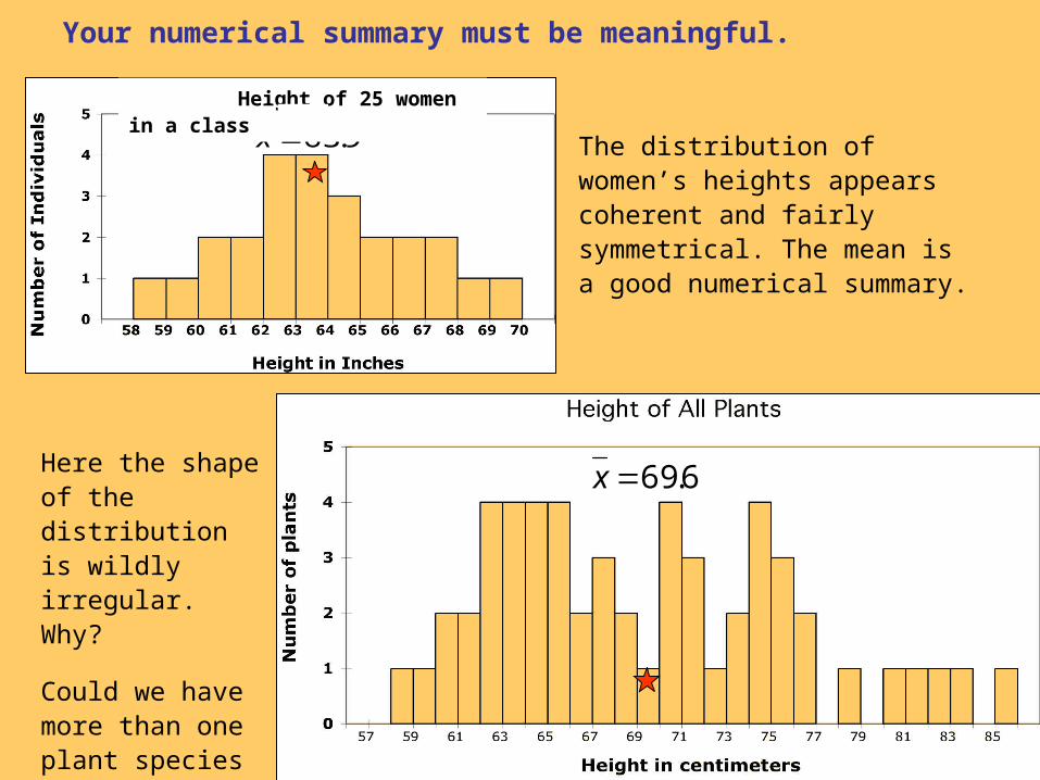
Your numerical summary must be meaningful.

Here the shape of the distribution is wildly irregular. Why?

Could we have more than one plant species or phenotype?

6.69x

The distribution of women’s heights appears coherent and fairly symmetrical. The mean is a good numerical summary.

9.63x Height of 25 women in a class

Height of Plants by Color

0

1

2

3

4

5

Height in centimeters

Num

ber of

Pla

nts

red

pink

blue

58 60 62 64 66 68 70 72 74 76 78 80 82 84

A single numerical summary here would not make sense.

9.63x 5.70x 3.78x

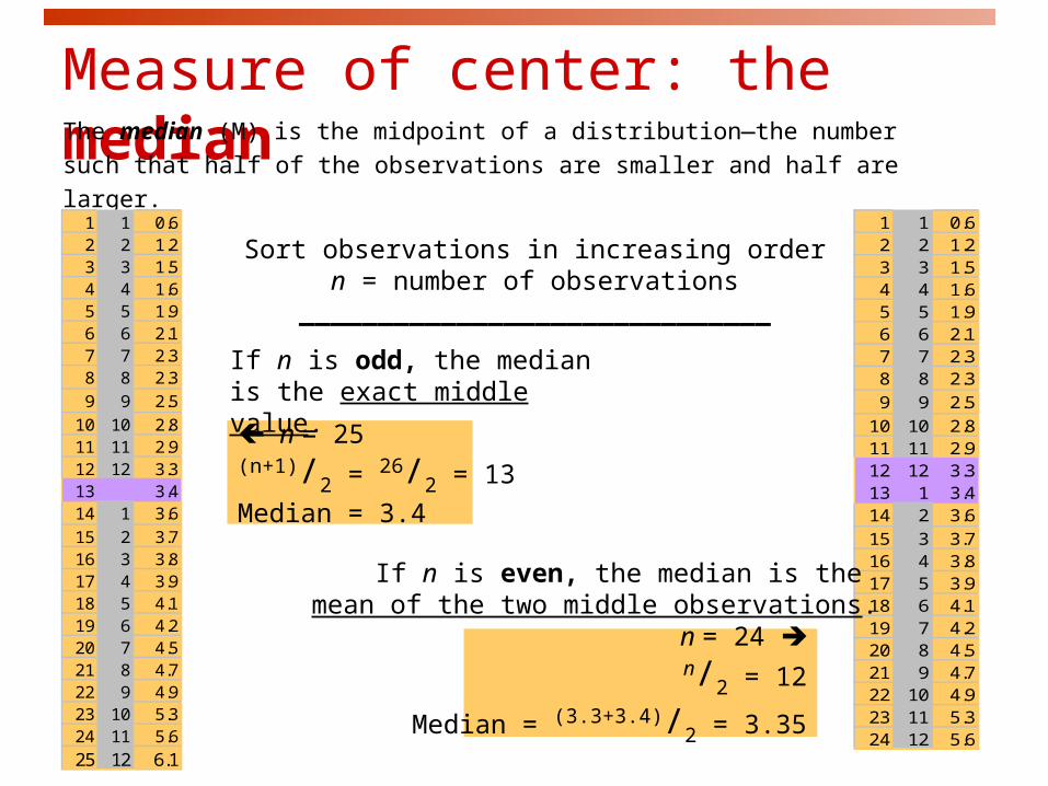
Measure of center: the medianThe median (M) is the midpoint of a distribution—the number such

that half of the observations are smaller and half are larger.

Sort observations in increasing ordern = number of observations

______________________________

1 1 0.62 2 1.23 3 1.54 4 1.65 5 1.96 6 2.17 7 2.38 8 2.39 9 2.510 10 2.811 11 2.912 12 3.313 1 3.414 2 3.615 3 3.716 4 3.817 5 3.918 6 4.119 7 4.220 8 4.521 9 4.722 10 4.923 11 5.324 12 5.6

n = 24 n/2 = 12

Median = (3.3+3.4)/2 = 3.35

If n is even, the median is the mean of the two middle observations.

1 1 0.62 2 1.23 3 1.54 4 1.65 5 1.96 6 2.17 7 2.38 8 2.39 9 2.510 10 2.811 11 2.912 12 3.313 3.414 1 3.615 2 3.716 3 3.817 4 3.918 5 4.119 6 4.220 7 4.521 8 4.722 9 4.923 10 5.324 11 5.625 12 6.1

n = 25 (n+1)/2 = 26/2 = 13

Median = 3.4

If n is odd, the median is the exact middle value.

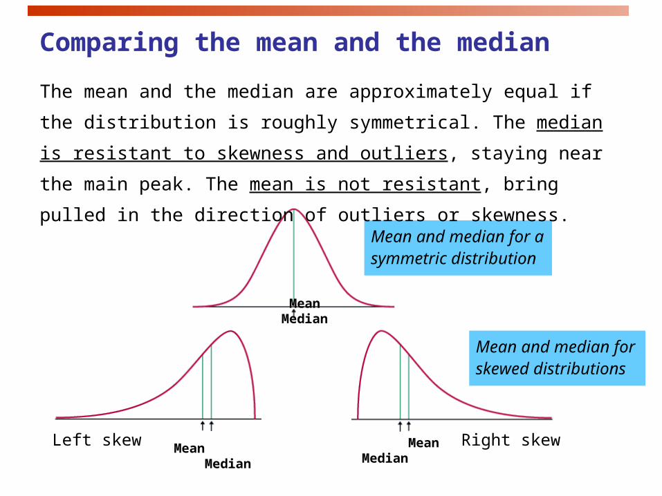
Mean and median for skewed distributions

Mean and median for a symmetric distribution

Left skew Right skew

MeanMedian

Mean Median

MeanMedian

Comparing the mean and the median

The mean and the median are approximately equal if the distribution is

roughly symmetrical. The median is resistant to skewness and outliers,

staying near the main peak. The mean is not resistant, bring pulled in

the direction of outliers or skewness.

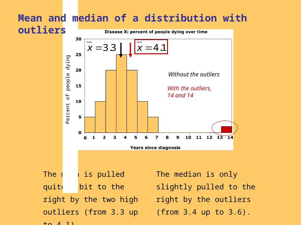
The median is only slightly

pulled to the right by the outliers

(from 3.4 up to 3.6).

The mean is pulled quite a bit

to the right by the two high

outliers (from 3.3 up to 4.1).

P

erc

en

t o

f p

eo

ple

dyi

ng

Mean and median of a distribution with outliers

3.3x

Without the outliers

1.4x

With the outliers, 14 and 14

Disease X:

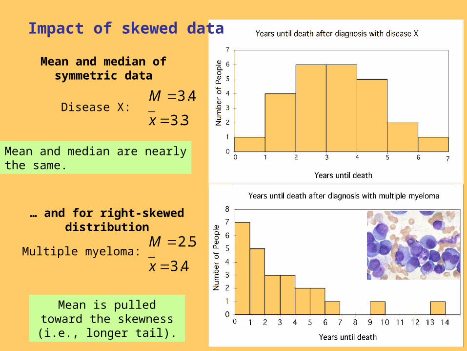
Mean and median are nearlythe same.

Mean and median of symmetric data

3.3

4.3

x

M

Multiple myeloma:4.3

5.2

x

M

… and for right-skewed distribution

Mean is pulled toward the skewness (i.e., longer tail).

Impact of skewed data

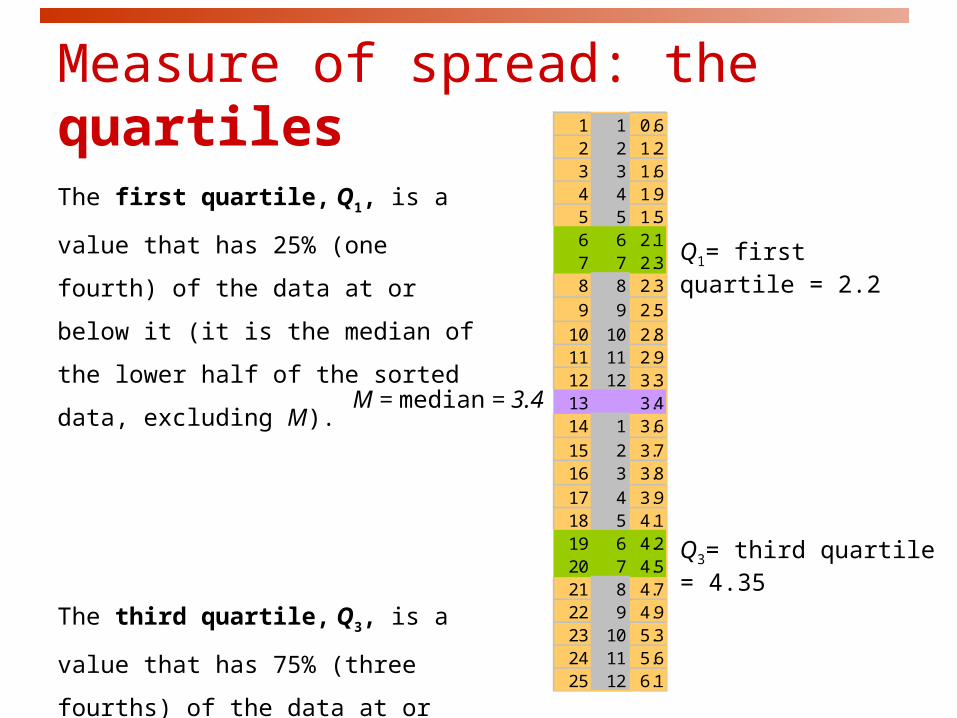
M = median = 3.4

Q1= first quartile = 2.2

Q3= third quartile = 4.35

1 1 0.62 2 1.23 3 1.64 4 1.95 5 1.56 6 2.17 7 2.38 8 2.39 9 2.510 10 2.811 11 2.912 12 3.313 3.414 1 3.615 2 3.716 3 3.817 4 3.918 5 4.119 6 4.220 7 4.521 8 4.722 9 4.923 10 5.324 11 5.625 12 6.1

Measure of spread: the quartilesThe first quartile, Q1, is a value that has

25% (one fourth) of the data at or below it

(it is the median of the lower half of the

sorted data, excluding M).

The third quartile, Q3, is a value that has

75% (three fourths) of the data at or

below it (it is the median of the upper half

of the sorted data, excluding M).

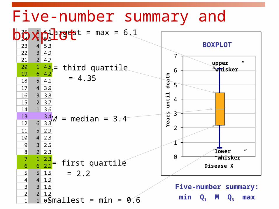
M = median = 3.4

Q3= third quartile = 4.35

Q1= first quartile = 2.2

25 6 6.124 5 5.623 4 5.322 3 4.921 2 4.720 1 4.519 6 4.218 5 4.117 4 3.916 3 3.815 2 3.714 1 3.613 3.412 6 3.311 5 2.910 4 2.89 3 2.58 2 2.37 1 2.36 6 2.15 5 1.54 4 1.93 3 1.62 2 1.21 1 0.6

Largest = max = 6.1

Smallest = min = 0.6

Disease X

0

1

2

3

4

5

6

7

Yea

rs u

nti

l dea

th

Five-number summary:

min Q1 M Q3 max

Five-number summary and boxplot

BOXPLOT

lower “whisker”

upper “whisker”

0123456789

101112131415

Disease X Multiple Myeloma

Yea

rs u

ntil

deat

h

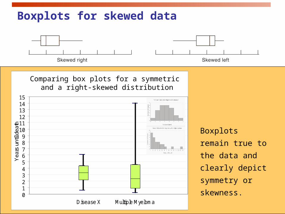
Comparing box plots for a symmetric and a right-skewed distribution

Boxplots for skewed data

Boxplots remain

true to the data and

clearly depict

symmetry or

skewness.

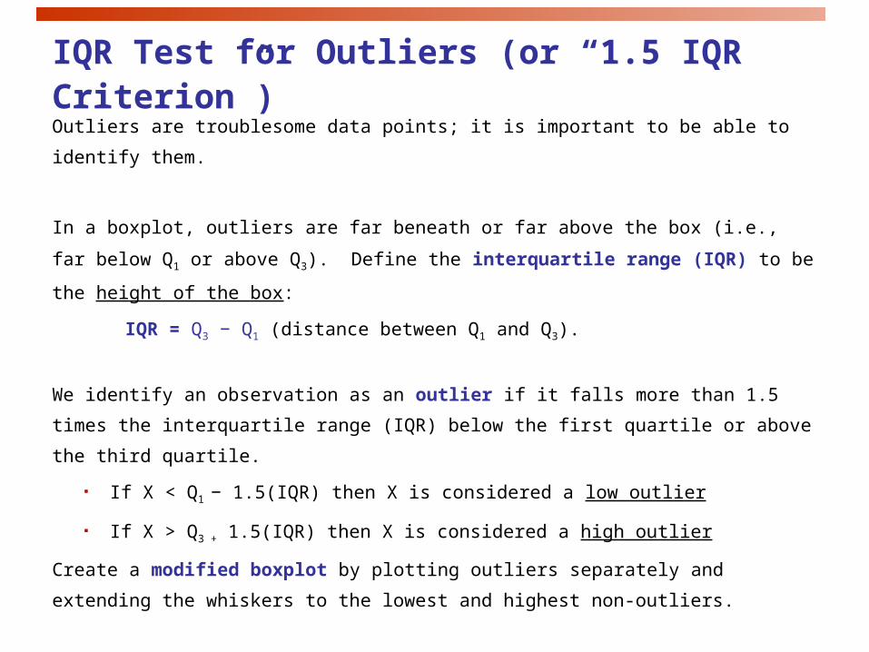
IQR Test for Outliers (or “1.5 IQR Criterion”)Outliers are troublesome data points; it is important to be able to identify them.

In a boxplot, outliers are far beneath or far above the box (i.e., far below Q1 or

above Q3). Define the interquartile range (IQR) to be the height of the box:

IQR = Q3 − Q1 (distance between Q1 and Q3).

We identify an observation as an outlier if it falls more than 1.5 times the

interquartile range (IQR) below the first quartile or above the third quartile.

If X < Q1 − 1.5(IQR) then X is considered a low outlier

If X > Q3 + 1.5(IQR) then X is considered a high outlier

Create a modified boxplot by plotting outliers separately and extending the

whiskers to the lowest and highest non-outliers.

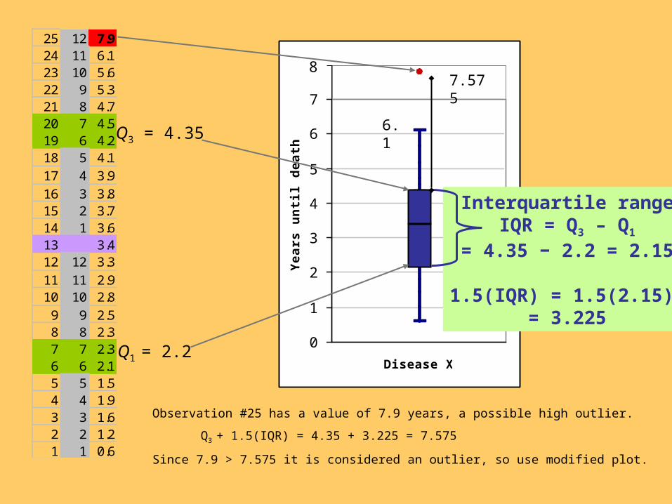
Q3 = 4.35

Q1 = 2.2

25 12 7.924 11 6.123 10 5.622 9 5.321 8 4.720 7 4.519 6 4.218 5 4.117 4 3.916 3 3.815 2 3.714 1 3.613 3.412 12 3.311 11 2.910 10 2.89 9 2.58 8 2.37 7 2.36 6 2.15 5 1.54 4 1.93 3 1.62 2 1.21 1 0.6

Disease X

0

1

2

3

4

5

6

7

Yea

rs u

nti

l dea

th

8

Interquartile rangeIQR = Q3 – Q1

= 4.35 − 2.2 = 2.15

1.5(IQR) = 1.5(2.15) = 3.225

Observation #25 has a value of 7.9 years, a possible high outlier.

Q3 + 1.5(IQR) = 4.35 + 3.225 = 7.575

Since 7.9 > 7.575 it is considered an outlier, so use modified plot.

7.575

6.1

Measures of variation or spread answer the question,

“How much is the data set as a whole spread out?”

Range – distance from smallest data value to largest

range = max – min

Highly sensitive to outliers since depends solely on

the two most extreme values.

Interquartile range

IQR = Q3 − Q1

Better than overall range since

Variance and standard deviation

Each measures variation from the mean.

Measures of spread: the standard deviation

The standard deviation (s) describes variation above and below the mean. Like the mean, it is not resistant to skewness or outliers.

2

1

2 )(1

1xx

ns

n

ii

1. First calculate the variance s2.

2

1

)(1

1xx

ns

n

ii

2. Then take the square root to get

the standard deviation s.

Standard deviation

x

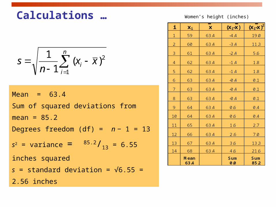
Calculations …

2

1

)(1

1xx

ns

n

ii

Mean = 63.4

Sum of squared deviations from mean = 85.2

Degrees freedom (df) = n − 1 = 13

s2 = variance = 85.2/13 = 6.55 inches squared

s = standard deviation = √6.55 = 2.56 inches

Women’s height (inches)

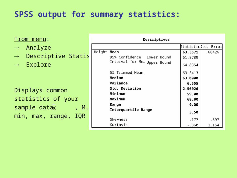
SPSS output for summary statistics:

From menu:

Analyze

Descriptive Statistics

Explore

Displays common

statistics of your

sample data: , M, s2, S,

min, max, range, IQR

Descriptives

63.3571 .68426

61.8789

64.8354

63.3413

63.0000

6.555

2.56026

59.00

68.00

9.00

3.50

.177 .597

-.360 1.154

Mean

Lower Bound

Upper Bound

95% ConfidenceInterval for Mean

5% Trimmed Mean

Median

Variance

Std. Deviation

Minimum

Maximum

Range

Interquartile Range

Skewness

Kurtosis

HeightStatistic Std. Error

x

Comments on standard deviation Standard deviation is generally positive (and never negative!)

(s = 0 only when data values are identical— not very interesting data!)

Larger standard deviation more variation in the data (i.e., data is spread out farther from the mean)

Standard deviation has the same units as the original data(while variance does not)

Choosing measures of center and spread:

Mean and standard deviation are more precise (since based on actual data values); have nice mathematical properties but not resistant.

Median and IQR are less precise (since based only on positions); are resistant to outliers, errors and skewness.

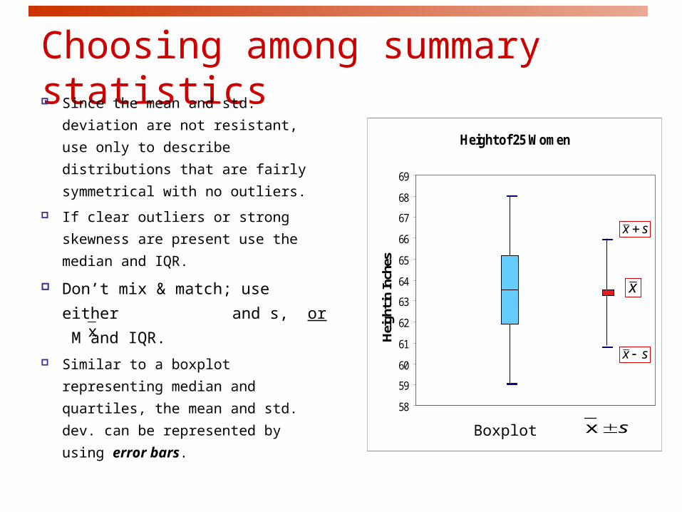
Choosing among summary statistics Since the mean and std. deviation

are not resistant, use only to

describe distributions that are fairly

symmetrical with no outliers.

If clear outliers or strong skewness

are present use the median and

IQR.

Don’t mix & match; use either

and s, or M and IQR.

Similar to a boxplot representing

median and quartiles, the mean

and std. dev. can be represented

by using error bars.

Height of 25 Women

58

59

60

61

62

63

64

65

66

67

68

69

Box Plot Mean +/- SD

Hei

ght i

n In

ches

Boxplot

x

sx

sx

sx

x

Mean or Median #1

Which should you use (and why) – mean or median?

Middletown is considering imposing an income tax on citizens. City

hall wants a numerical summary of its citizens income to estimate

the total tax base.

In a study of standard of living of families in Middletown, a

sociologist desires a numerical summary of “typical” family income in

that city.

Mean or Median #2

You are planning to buy a home in Middletown. You ask your real

estate agent what the “average” home value is in the neighborhood

you are considering.

Which would be more useful to you as the home buyer – the

mean or the median?

Which might the real estate agent be tempted to tell you is the

“average” home value? Why?

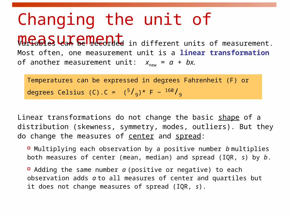
Changing the unit of measurementVariables can be recorded in different units of measurement. Most often, one measurement unit is a linear transformation of another measurement unit: xnew = a + bx.

Temperatures can be expressed in degrees Fahrenheit (F) or degrees

Celsius (C). C = (5/9)* F − 160/9

Linear transformations do not change the basic shape of a distribution (skewness, symmetry, modes, outliers). But they do change the measures of center and spread:

Multiplying each observation by a positive number b multiplies both measures of center (mean, median) and spread (IQR, s) by b.

Adding the same number a (positive or negative) to each observation adds a to all measures of center and quartiles but it does not change measures of spread (IQR, s).

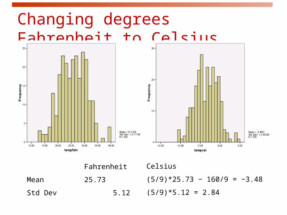
Changing degrees Fahrenheit to Celsius

Fahrenheit

Mean 25.73

Std Dev 5.12

Celsius

(5/9)*25.73 − 160/9 = −3.48

(5/9)*5.12 = 2.84