Longitudinal Motion Control of a High-Speed ... · Longitudinal Motion Control of a High-Speed...

Longitudinal Motion Control of a

High-Speed Supercavitation Vehicle

Balint Vanek ([email protected])∗, Jozsef Bokor([email protected])† and Gary J. Balas ([email protected])Aerospace Engineering and Mechanics, 110 Union St. SE, University ofMinnesota, Minneapolis, MN 55455

Roger E.A. Arndt ([email protected])Civil Engineering and St. Anthony Falls Laboratory, 2 Third Ave. SE, Universityof Minnesota, Minneapolis, MN 55414

June 15, 2006

Abstract. This article focuses on theoretical developments in modeling and controlof High-Speed Supercavitating Vehicles (HSSV). A simplified model of longitudinaldynamics is developed for control, and a dynamic inversion based inner-loop con-trol technique is proposed to handle the switched, time-delay dependent behaviorof the vehicle. Two outer-loop control schemes are compared for guidance leveltracking. Various aspects of disturbance characteristics and actuator dynamics areinvestigated and analyzed.

Keywords: supercavitation, dynamic inversion, bimodal systems, receding horizoncontrol

Figure 1. Water tunnel experiment on supercavitation

1. Introduction

Cavitation is an undesired phenomena in most engineering applications.Recent developments in supercavitation, motivated by the demand for

∗ corresponding author† on sabbatical leave from MTA SZTAKI, Hungarian Academy of Sciences,

Budapest XI. Kende u. 13-17, H-1518 Budapest, POB 63, Hungary

c© 2006 Balint Vanek. University of Minnesota.

JVC06-12.tex; 26/08/2006; 17:12; p.1

2 B. Vanek, J. Bokor, G.J. Balas and R.E.A. Arndt

high-speed underwater vehicles (DARPA Advanced Technology Of-fice, 2005; Ashley, 2001) has generated renewed interest in cavitation.Supercavitation can provide significant benefit for drag reduction bymaintaining a stable single vaporized water bubble around the ve-hicle making it possible to extend the velocity range of underwaterapplications.

The sharp edge of a cavitator mounted on the nose of the vehiclecreates large pressure gradient at high velocity. This phenomena leadsto flow separation, which can create a cavity bubble encompassing theentire body. Only small regions of the vehicle are in contact with water.The cavitator and fins at the aft end (if present) provide lift to stabi-lize the body and may be used for guidance level control tasks. Thecavitator size, shape and forward velocity determine the dimensions ofthe cavity bubble in which the body must fit. Any other contact withfluid phase is undesirable from a drag reduction standpoint. In thisvehicle configuration, with no additional lift components, the vehicle isunstable inside the cavity. One means to address the vehicle stabilityinvolves the body itself. When the aft end penetrates the cavity surface,a large restoring force, known as planing, forces the vehicle back insidethe cavity. Planing can be used as a support force to improve maneu-verability and eliminate the need for fins. This leads to a reduced costand system complexity, but it can also lead to limit cycle oscillationsand increased drag if not controlled.

The actuation of the cavitator mounted on the nose becomes prob-lematic if the goal is not only longitudinal control but three dimensionaltrajectory tracking. The influence of high cavitator actuation rate onthe cavity stability and shape is uncertain. If planing does not supportthe vehicle weight, then fins at the aft end have to provide a lift forceto balance the moment and stabilize the pitch motion. The fins effec-tiveness is a nonlinear function of their immersion depth, and planingcan also occur with actively controlled fins. Note that the gap betweenthe body and the cavity wall is on the order of 1 − 5 cm comparedto the body length of 1− 2 meters, for vehicle speeds between 75 and100 m/s. Cavity-vehicle interaction also has memory effects since thecavity shape, which affects planing, is a function of the vehicle pastpath and buoyancy. Suppression of limit cycle oscillations and distur-bance attenuation require high bandwidth actuators, precise inertialmeasurements, and high sample rate real-time control algorithms.

The Russian navy has a supercavitation vehicle, the Shkval, cur-rently in operation (Ashley, 2001), and German Diehl BGT Defence hasdemonstrated successful stable, straight and curved path maneuverswith the Barracuda (www.diehl-bgt-defence.de) supercavitating ve-hicle. Despite these successes, no solution to the three dimensional

JVC06-12.tex; 26/08/2006; 17:12; p.2

Longitudinal Motion Control for HSSV 3

trajectory tracking problem for supercavitating vehicles is availablein the open literature. Significant research on supercavitation vehiclecontrol has been done in the past years, mostly using linear regulators((Shao et al., 2003; Goel, 2002; Kirschner et al., 2002b; Kurdila et al.,2003)). These model-based designs rely on linearized dynamics aroundoperating points. None of these approaches provide a planing-free op-eration which is a potential requirement in the future UnderwaterExpress program ((DARPA Advanced Technology Office, 2005)). Othercontrol approaches, using nonlinear techniques ((Dzielski and Kurdila,2003; Lin et al., 2004)) are in the early development phase. Numerouschallenges face the designers of supercavitating vehicle control systems.

This paper focuses on control challenges associated with the longi-tudinal axis motion of supercavitating vehicles. The first part of thepaper (Section 2) describes a simplified pitch-plane model of a HSSV.This model is a refined version of the model described in (Vanek et al.,2006a), which was motivated by the papers of Dzielski and Kurdila(2003) and Kirschner et al. (2003). The model includes delay-dependentinteraction between the vehicle and cavity wall, pitch-angle-dependentterms, and a refined planing model. In contrast with previous mod-els, the equations of motion are written around the center of gravity.The second part of the paper summarizes the theoretical results onbimodal systems, which enable the systematic design of a dynamic-inversion-based inner-loop control architecture (Section 3). An outer-loop controller is added to guarantee high-level tracking objectives. Inthis paper, a pole-placement trajectory tracking controller with ver-tical position and pitch-angle-tracking objectives is compared with areceding horizon control (RHC) based design, where position and angletracking, planing avoidance, and actuator saturation are formulated asperformance objectives.

This paper adds to the literature by adressing planing avoidanceas a performance objective. Linear control methods previously pro-posed ((Goel, 2002),(Shao et al., 2003)) did not take into account thelarge deviations from the nominal equations of motion, hence stabilityand performance were not guaranteed when the vehicle was planing.Nonlinear methods proposed by ((Dzielski and Kurdila, 2003),(Vaneket al., 2006b)) guarantee stability during planing, using the controlsurfaces to attenuate the large forces caused by planing, but do nottake into account actuator position and rate limits, which restricts theoperation envelope of the vehicle. The result of this research show thatplaning avoidance as a performance objective can significantly expandthe operation envelope of the HSSV. The increased performance comesat the expense of slightly degraded position tracking performance, whileplaning with undesirably high acceleration happens seldom if ever.

JVC06-12.tex; 26/08/2006; 17:12; p.3


Simulation results of the closed-loop systems are compared in Sec-tion 5. Challenges facing the control designer are highlighted with re-spect to the actuator and sensor requirements, modeling issues, vehicleconfiguration, robustness and performance. Conclusions and future di-rections emphasizing the most important design criteria are highlightedin the last section.

2. Mathematical Model

Several mathematical descriptions are available in the literature ofsupercavitating vehicles, ranging from vertical directional one degree-of-freedom (DOF) model (Kirschner et al., 2003), through a simplified2-DOF longitudinal description (Dzielski and Kurdila, 2003) to a highfidelity 6-DOF model (Kirschner et al., 2002a). A broader overview onthe characteristics of these models can be found in (Balas et al., 2006)where another 2-DOF model from (Vanek et al., 2006a) is described.

Delay-dependent behavior of the cavity with refined treatment ofplaning was developed in (Vanek et al., 2006b), however it neglected thecontrol forces’ pitch angle dependence. Given a single control surfacean additional force to support the vehicle requires constant nonzeropitch angle of the vehicle. Hence, a relationship between the pitchangle, moments and forces need to be developed. This is apparent sincetrimming the vehicle around straight level flight requires nonzero angleof attack on the fins and cavitator, to generate the required force andmoment balance.

For simplicity, the equations of motion are written around the centerof gravity (c.g.) and small angle approximations are used to eliminatetrigonometric nonlinearities. The small angle assumption is valid sincewe anticipate angles less than 0.2 rad. Variable definition and coordi-nate directions are shown in Figure 2. The geometry of the model isintended to capture the main characteristics of a test vehicle. The bodyconsists of a cylindrical and a conical section, with the length of thelatter half of the former. The reference coordinate system is placed atthe center of gravity with positive x-axis pointing in forward horizontaldirection and the z-axis pointing to the center of Earth. The pitch angleis denoted by θ (rad), pitch rate q (rad/s), the vertical position z (m)and vertical velocity is w (m/s). δc (rad) is the cavitator angle withrespect to the x body axis, and δf (rad) the fin angle of attack in thebody coordinates. In general, there are four forces acting on the body,the cavitator and fins forces, gravity, and planing which is not alwayspresent.

JVC06-12.tex; 26/08/2006; 17:12; p.4


The body length is denoted by L (m) and its radius is R (m). Thebody has uniform density ρb = ρm (kg/m3), with relative density mcompared with water (ρ), from which the mass and inertia can becalculated, neglecting the cavitator and fins contribution. Hence, thevehicle mass (M), moment of inertia around the y axis (Iyy) and centerof gravity location from the nose (xcg) are given as:

M =79(mρπ)R2L (1)

Iyy =1160

R4Lπρm +193345360

R2L3πρm (2)

xcg =1728

L (3)

If the full vehicle body is inside the cavity, hydrodynamic forces only

Cavity envelopeCavity centerline

Torpedo’s symmetry line

immersion

immersionfin

cav

plane

fin

g

cav

Figure 2. Variables in the longitudinal plane

act on the cavitator and the fins. The cavitator drag coefficient ismodeled as Cx = Cx0(1 + σ) where σ is the cavitation number andCx0 = 0.82 (Logvinovich, 1972). The resulting lift on the cavitator isapproximately:

Fcav =12πρR2

nV 2Cxαc = Clαc (4)

where Rn (m) is the cavitator radius, ρ the water density, V (m/s) thevehicle’s horizontal speed, and αc is the cavitator angle of attack. Theforce acting on the fins located at the tail is modeled as:

Ffin = nClαf (5)

where n represents the fins effectiveness in providing lift as a function ofangle of attack (αf ) relative to the cavitator. Note that in the longitudi-nal plane, the two horizontal fins are assumed to move in unison. Only

JVC06-12.tex; 26/08/2006; 17:12; p.5


small angle deflections with maximum value of 0.2 rad are considered.The following simplifying assumptions are assumed through out thispaper: the horizontal velocity (V ), water density (ρ) and cavitationnumber (σ) are assumed constant.

The force and moment equations around the c.g. using the conven-tions shown in Figure 2 are written as:

Mw = Fcav + Ffin + Fg + Fp (6)

Iyy q = −(FcavLc + FfinLf + FpLf ) (7)

where Lc = 17/28L and Lf = −11/28L are the respective momentarms of the cavitator and fin forces. The planing force is assumed toact at −Lf distance from the c.g. The force components as function ofvehicle states are:

Fcav =12πρR2

nV 2Cl(w

V− qLc

V+ θ + δc) (8)

Ffin = −12πρR2

nV 2Cln(w

V− qLf

V+ θ + δf ) (9)

Fg =79ρmπR2Lg (10)

The remaining term Fp associated with the planing force needs furtherconsideration. This force is present when the vehicle transom interactswith the cavity wall, leading to a force similar to that sustained bypowerboats bouncing on the top of the water. In the particular case ofthe HSSV, the free fluid surface is the circular cavity wall created bythe cavitator and the vehicle tail is tubular. Logvinovich (1972) andVasin and Paryshev (2001) analyzed the situation when a cylindricalbody immerses into a cylindrical free fluid surface, which applies tothe current vehicle configuration. These analytical results relate theimmersion depth h (m) and the distance from the axis of symmetry tothe narrowest part of the spray sheet, generated by the displaced fluid.

The pressure force on the body is calculated from the energy of thespray sheet. If the diameter of the cavity at the planing location is Rc,then for (Rc−R) << Rc and small immersion angles, the planing forcecan be approximated as:

Fp = −ρR2πV 2(

1− R′

h′ −R′

)2 ( 1 + h′

1 + 2h′

)αp (11)

The variable R′ denotes the normalized difference between the cavityand body diameter (R′ = (Rc − R)/R). The variables h′ the nor-malized immersion depth and αp (rad) the immersion angle, capture

JVC06-12.tex; 26/08/2006; 17:12; p.6


the switched, nonlinear behavior of the dynamics. From Figure 2, theplaning depth is determined by the cavity shape (as a function of thecavitator trajectory), vehicle position, and orientation. The position ofthe vehicle transom, where planing occurs, is a function of the vehicleposition, rotation, and vehicle radius at the transom.

The cavity boundary is located at Rc distance from its centerline,which is determined by the vehicle nose path through the water. Atthe transom region, the centerline is at zn(t− τ). The cavity radius atthe planing location is assumed to be constant. Hence, the immersiondepth is the difference between the two quantities, and the nose positionzn(t) = z(t)− Lcθ(t).

h′ =

1R

[z(t) + θLf + R− zn(t− τ)−Rc] if zn(t− τ) + Rc < z(t) + θLf + R

0 (inside cavity)

1R

[zn(t− τ)−Rc − z(t)− θLf + R] if zn(t− τ)−Rc > z(t) + θLf + R

(12)

Following the same reasoning, the immersion angle can be calculatedbased on the knowledge of the delayed vertical speed of the vehiclenose (zn(t) = w(t) − V θ(t) − Lcq(t)) and current pitch angle plus thecontraction rate of the cavity bubble (Rc):

αp =

θ − zn(t−τ)+Rc

V bottom contact

0 inside cavity

θ − zn(t−τ)−Rc

V top contact

(13)

It is important to note that, based on equation (12) the system isdescribed by three different set of equations corresponding to threepossible modes, one with linear and the other two with nonlinear delaydependent terms. The vehicle dynamics are continuous on the switchingsurface between different modes, since the nonlinear planing force iszero on the boundary.

Stability and hysteresis tests with a cavity-piercing fin performed inthe high-speed water tunnel at St. Anthony Falls Laboratory (Syrstadet al., 2005) confirm the cavity shape specification as described in(Logvinovich, 1972). To simplify further the dynamic equations basedon the assumption that the body planes at the approximate locationof the fins, the following constants are defined:

κ1 =L

Rn(1.92σ

− 3)−1 − 1, κ2 = (1− (1− 4.5σ

1 + σ)κ

40171 )

12 (14)

JVC06-12.tex; 26/08/2006; 17:12; p.7


Using the above expressions, the radius of the cavity at L distance fromthe cavitator is:

Rc = Rn(0.821 + σ

σ)

12 κ2 (15)

The expression for the contraction rate of the cavity (Rc) is:

Rc = −2017

(0.821 + σ

σ)

12 V

(1− 4.5σ1+σκ

23171 )

κ2(1.92σ − 3)

(16)

The equations for the cavity shape presented in equation (16) are validgiven that they are evaluated sufficiently far from the cavitator:

L > Rn(1.92σ

− 3) (17)

but before the cavity closure.Using these equations, supplemented by the basic kinematic equa-

tions for position and pitch angle:

θ = q, z = w − V θ (18)

the system states z, θ, w and q can be written in state space form as:z

θwq

= A

zθwq

+ B

[δe

δc

]+ Fgrav + Fplane(t, τ) (19)

where A and B represent the linear part, Fgrav is a constant termand Fplane corresponds to the nonlinear relationship associated withplaning. The specific values of the system matrices are as follows:

A =

0 −V 1 00 0 0 10 (C1−C2)

M(C1−C2)(MV )

(−C1Lc+C2Lf )(MV )

0 (−C1Lc+C2Lf )Iyy

(−C1Lc+C2Lf )(IyyV )

(C1L2c−C2L2

f )

(IyyV )

(20)

B =

0 00 0C1M

C2M

−C1Iyy

LcC2Iyy

Lf

(21)

Fgrav =

00g0

(22)

JVC06-12.tex; 26/08/2006; 17:12; p.8


Table I. System parameters for simulation model

Parameter Description Value and Units

g Gravitational acceleration 9.81 ms2

m Density ratio, ρmρ

2

n Fin effectiveness 0.5

Rn Cavitator radius 0.0191 m

R Vehicle radius 0.0508 m

L Length 1.80 m

V Velocity 75 ms

σ Cavitation number 0.03

Cx0 Lift coefficient 0.82

Fplane =

00Cp

M

− Cp

IyyLf

(

1− R′

h′(t, τ)−R′

)2 ( 1 + h′(t, τ)1 + 2h′(t, τ)

)αp(t, τ) (23)

The constant terms C1, C2, Cp are defined to simplify the presentation.Their specific values are:

C1 =12πρR2

nV 2Cx, C2 =12πρR2

nV 2Cxn, Cp = πρR2V 2 (24)

The system parameters are based on the benchmark HSSV in (Dzielskiand Kurdila, 2003) and presented in Table I.

3. Theoretical aspects of controller design

The state space equations describing the system in equation (19) rep-resent a bimodal switched system. Several characteristics of this modelare of interest: (i) in the first mode, the system dynamics are linear(inside cavity), and in the second mode they are nonlinear (planing)input affine, though the control inputs affect the dynamics linearly inboth modes, (ii) the switching condition does not depend on the con-trol inputs, and (iii) the switching hyperplane depends on the delayedoutput variable zn(t− τ).

A switched, hybrid control strategy was developed in Balas et al.(2006) for this type of system. Properties (i) and (ii) allow for feedback

JVC06-12.tex; 26/08/2006; 17:12; p.9


linearization in both modes. This is performed via a coordinate systemwith suitable geometric structure for the problem. It was shown (Balaset al., 2006) that this design results in linear dynamics in both modesensuring continuous dynamics on the switching hypersurface. Since thelatter depends on delayed state variables, controllability has to be an-alyzed, and a controller has to be designed that ensures stability andtracking performance.

The proposed approach relies on the assumption that the delayin the equations of motion can be eliminated by applying a suitablefeedback. The resulting controllability analysis and control design canthen be performed for bimodal linear time invariant (LTI) systems.

New state variables for equation (19) are selected for analysis andcontrol design:

x1(t)x2(t)x3(t)x4(t)

=

zn(t)

−V θ(t) + wn(t)θ(t)q(t)

(25)

The matrix used for this coordinate transformation is:

Tc =

c1

c1Ac2

c2A

=

1 −Lc 0 00 −V 1 −Lc

0 1 0 00 0 0 1

(26)

The state space equations in the new coordinate system are:

˙x =

{Acx(t) + Bcu(t) + Fg if c(δ)x(t) ≤ 0,

Acx(t) + Fp(t, x, δ) + Bcu(t) + Fg if c(δ)x(t) ≥ 0,(27)

where

Ac =

0 1 0 0

−α110 −α111 −α120 −α121

0 0 0 1−α210 −α211 −α220 −α221,

Bc =

0

c1AB0

c2AB

(28)

The difference between Fgrav and Fgrav is that Fgrav = TcFgrav + K1

where K1 is a constant associated with the shift in the origin of thecoordinate system. Similarly Fplane = TcFplane.

The inputs enter linearly in the state equations in both modes, andit is assumed that all states can be measured. This allows us to selecttwo outputs defined as y1 = x1 and y2 = x3, such that the vector

JVC06-12.tex; 26/08/2006; 17:12; p.10


relative degree is well defined in both modes, and in addition, they areidentical, i.e. by defining:

Cc =[1 0 0 00 0 1 0

](29)

The relative degree for the modes are:

r21 = 2, r1

2 = 2, r21 + r1

2 = n = 4 Mode 1 (30)

r21 = 2, r2

2 = 2, r21 + r2

2 = n = 4 Mode 2 (31)

The consequence of this property is that one can apply state feed-back in both modes to eliminate the time delay in Mode 1 and thenonlinearity (exact feedback linearization) in Mode 2 (Balas et al.,2005b). This feedback is given by (Balas et al., 2006):

Vehicle

fincavitator

Feedback Linearizing Controller

cB.Actv

gravF 0x

∫ sC

cA

planeF

δ

(Bimodal)

sy

(switching) Linear system

x (t-_

x_

Figure 3. Control architecture for supercavitating vehicle model

uflc =

{M−1

1 (y12,ref (t)− Fαx(t)− Fg + vI(t)) if c(δ)x(t) ≤ 0,

M−11 (y12,ref (t)− Fαx(t)− Fg − Fp(x, δ) + vII(t)) if c(δ)x(t) ≥ 0,

(32)where M1 = (CAB), y12,ref = [y1, y2]Tref . The feedback gain Fα is

defined by the controllability invariants αijk of the linear part of thesystem (equation (28)). The structure of the designed feedback systemis shown in Figure 3.

JVC06-12.tex; 26/08/2006; 17:12; p.11


The feedback linearized closed-loop has the following form in bothmodes:

˙x =

0 1 0 00 0 0 00 0 0 10 0 0 0

x +

0 01 00 00 1

[v1

v2

](33)

The switching condition is given by the sign of ys = c(δ)x.

3.1. Controllability analysis of the bimodal system

Controllability of linear bimodal systems with single input and dy-namics continuous on the switching surface is analyzed in (Camlibelet al., 2004). These results are generalized to multi-input systems in(Balas et al., 2005b) and applied to the supercavitating vehicle in (Balaset al., 2006). The results show that the controllability analysis can beperformed by analyzing the controllability of the zero dynamics of theswitched system with respect to the switching hyperplane (C).

It can be shown that every linear system with relative degree (r) andswitching output ξ1 = ys has the following decomposition by applyingstate transform and state feedback:

ξ = A11ξ + γv (34)

up =1γ

(−A12η − B21u + v) (35)

η = A22η + B22u + Gys, (36)

Since ξ1 = ys, equation (36) describes the dynamics of the systemon C. Rewrite the equation of this zero dynamics as:

η = Pη + Qu + Rys. (37)

It is proved in (Balas et al., 2005b) that either the pair (P,Q) hasto be controllable, then η is controllable “without” using ys, e.g. byapplying u = Q#(−Rys + w), or if the pair (P,Q) is not controllable,then the conditions of controllability of the bimodal switching systemreduces to the controllability of equation (37) using unconstrained uand nonnegative (or in the other mode non-positive) input ys: (i) Thepair (P, [QR]) has to be controllable, (ii) Consider the decompositionof equation (37) induced by the reachability subspace R(P,Q),

η1 = P11η1 + P12η2 + Qu + R1ys (38)η2 = P22η2 + R2ys, (39)

where R2 6= 0. Then the imaginary part of the eigenvalues of P22 cannotbe zero.

JVC06-12.tex; 26/08/2006; 17:12; p.12


For the high-speed supercavitating vehicle model, this result hasto be generalized for a time delay system. Since only one delay timeis present in the switching condition, it is possible to discretize thesystem using backward difference approximation (Safonov, 1987) thatpreserves the relative degree needed to analyze the zero dynamics, withextended state space by including the delayed state variable.

This results in the following discrete time state equations:

x(t + 1) = Adx(t) + Bdv(t), ys = Cdx(t) (40)

where

Ad =

1 T 0 0 00 1 0 0 00 0 1 T 00 0 0 1 01 0 0 0 0

, Bd =

0 0

β21T β22T0 0

β41T β42T0 0

, Cd = [1, 0, V, 0,−1].

(41)T denotes the sample time and the fifth state is the delayed position

of the cavitator. The switched output (Cd) is derived based on equation(12). The above system can be decomposed into the following set ofequations:

ξ(t+1) =[0 a12

0 a22

]ξ(t)+

[0 0 00 b22 b23

]η(t)+

[0

e21

]v1(t)+

[0

e22

]v2(t) (42)

ys =[1 0

]ξ(t) switching condition (43)

η(t + 1) = Pη(t) + Rξ(t) + Qv2(t), (44)

where

P =

p11 p12 p13

0 p22 p23

0 0 p33

, R =

0 r12

0 r22

0 0

, Q =

00

q31

. (45)

The zero dynamics with respect to the first input v1 are describedby equation (44) and a similar decomposition can be obtained withrespect to v2. Using the results in (Balas et al., 2006), it can be seenthat the (P,Q), pair is controllable in both cases, implying that thedynamic inversion controller using inputs v1 and v2 with switchingcan be applied to control the bimodal system and an additional linearcontroller can be used for trajectory tracking.

JVC06-12.tex; 26/08/2006; 17:12; p.13


4. Outer loop control strategy

A single, linear outer-loop controller can guarantee stability and achievethe desired tracking properties with feedback linearization, since thesystem behaves the same regardless of the interior switching state.A variety of linear design approaches can be used for stability andcontrol (Doyle et al., 1989; McFarlane and Glover, 1992; Balas et al.,2005a; Mayne et al., 2000). The ability of the controller to directlyhandle constraints could provide significant benefits if planing is re-stricted. Hence, a simple pole placement controller is compared withreceding-horizon control approach which allows for actuator and stateconstraints.

The inner loop dynamics after feedback linearization, using the newcanonical coordinates are:

x1

x2

x3

x4

=

0 1 0 00 0 0 00 0 0 10 0 0 0

x1

x2

x3

x4

+ Bc

[∆δf

∆δc

](46)

where ∆δf,c denotes the additional deflection of the fins and cavitatorcommanded by the higher level controller. This system is nilpotent,because all eigenvalues of A are zero. There is no cross coupling be-tween the first two states (vertical position and speed), and the otherstates (vehicle angle and angle rate). Hence, they can be controlledindependently by the two control inputs.

4.1. Multivariable Pole Placement for Tracking

An easy and tractable control design approach for linear systems ispole placement. The performance objective is to track desired statecommands with no restrictions on the maximum actuator deflections,since the tracking signals have minor contribution compared with theaction due to planing. With the assumption of full state feedback, thiscan be done fairly simply. The inversion based controller has the form:[

u1(t)u2(t)

]= (CAB)−1(−[αu]

[x1(t)x2(t)

]−

− [αl][x3(t)x4(t)

]− [Gc]− [Pc(t, τ)]) +

[∆δf

∆δc

](47)

Where the αu,l coefficients are the elements of the Ac matrix (equation(28)) and ∆δf,c are the signals responsible for reference tracking.

[αu] =[−α110 −α111

−α210 −α211

][αl] =

[−α120 −α121

−α220 −α221

](48)

JVC06-12.tex; 26/08/2006; 17:12; p.14


The reference tracking part of the controller responsible for pole loca-tions:

[∆δf

∆δc

]= (CAB)−1

{[−α110 −α111

0 0

] [x1(t)− x1,ref (t)x2(t)− x2,ref (t)

]+

+[

0 0−α220 −α221

] [x3(t)− x3,ref (t)x4(t)− x4,ref (t)

]+[x1,ref

x3,ref

]}(49)

The feedback linearized closed loop has the following form in allmodes:

Acl = Ac − BcFinv + BcFctr =

0 1 0 0

−α110 −α111 0 00 0 0 10 0 −α220 −α221

(50)

The closed-loop system is stable for a given set of α coefficients.

Feedback linearized system

∫cT pplF

FLA

FLBrefx

FLxv 1−cT

xdtd

11−M

Figure 4. Control architecture for supercavitating vehicle model

The tracking part of the controller is responsible for the location ofthe poles. The eigenvalues of the system are:

λ1,2 = −0.5α221 ± 0.5√

(−α221)2 − 4α220 (51)

λ3,4 = −0.5α121 ± 0.5√

(−α121)2 − 4α120

The poles can be freely adjusted in the stable region, while the driv-ing factor for actuator deflections remains planing cancelation. Hence,the only limiting factor for setting the pole locations is the actuatorbandwidth.

The structure of the feedback controller is shown in Figure 3. Theinner-loop controller feedback linearizes the system, and the outer-loop

JVC06-12.tex; 26/08/2006; 17:12; p.15


controller handles reference tracking. It is possible to track both posi-tion and angle commands with consistent position, velocity, angle andangle rate reference signals. The designed pole placement controller alsooperates on the transformed canonic coordinates. The special structureof the feedback linearized system allows the vehicle position and angleto be controlled independently.

4.2. Outer-Loop RHC control

This section describes the design of an outer-loop controller using Re-ceding Horizon Control (RHC). The previous section focused on theinner-loop control with a simple pole-placement controller to achievereference tracking properties. In addition to the performance specifica-tions, the reference tracking control should avoid actuator saturationand immersion into the fluid, preventing the inner loop to commandunrealistically high deflections to cancel out the forces generated byplaning. Predicting planing may provide beneficial information whichcan broaden the stable operation envelope of the vehicle, enabling moreaggressive reference trajectories, at the expense of slightly degradedtracking performance.

A popular way to avoid saturations on the actuators is to use pre-diction based control methods (Receding Horizon Control or ModelPredictive Control). The proposed control scheme is shown in Figure5.

Feedback linearized system

∫cT

FLA

FLBrefx

FLxv 1−cT

x

Performance objectives

RHC

Figure 5. The RHC control loop structure

The controller structure differs from the controller discussed in (Balaset al., 2006), as the outer-loop uses RHC technique (equation 52).[u1(t)u2(t)

]= (CAB)−1

(−[αu]

[x1(t)x2(t)

]− [αl]

[x3(t)x4(t)

]− [Gc]− [Pc(t, τ)]−

[v1,RHC(t)v2,RHC(t)

])(52)

The standard linear RHC problem and solution using quadratic pro-gramming is well known (Maciejowski, 2002) and reliable software tools

JVC06-12.tex; 26/08/2006; 17:12; p.16


are available for controller design (Bemporad et al., 2005). The discretetime controller is obtained in a receding horizon fashion using model-based predictions by solving a finite time constrained optimizationproblem:

min∆u(k|k),...,∆u(m+k−1|k),ε

{p−1∑i=0

(ny∑j=1

∣∣wyi+1,j(yj(k + i + 1|k)− rj(k + i + 1))

∣∣2 +

+

nu∑j=1

∣∣w∆ui,j ∆uj(k + i|k)

∣∣2 +

nu∑j=1

∣∣wui,j(uj(k + i|k)− uj,des(k + i))

∣∣2)+ ρεε2

}(53)

where ∆u denotes the input increments, (k+i|k) indicates the value fortime k+i using the available information at k. The tracking is achievedby minimizing the error between y(k + i|k) the predicted output andthe reference (r(k + i)). The actuator usage and input rates are alsoweighted in the cost function with wi,j coefficients. The constraints oninputs, input rates, or outputs can be implemented as soft constraints:

uj,min(i)− εV uj,min(i) ≤ uj(k + i|k) ≤ uj,max(i) + εV u

j,max(i) (54)

where ε is the slack variable relaxed with weight V uj , which is heavily

penalized in the cost function with ρε. Normally input constraints areimplemented as hard constraints while output constraints are softenedto ensure feasibility when large disturbances are expected. The predic-tion (ny) and control horizons (nu) have large impacts on the solutionand computational requirements. In general the prediction does notexactly match the system response. Hence, the best solution is oftenobtained by a suitable finite prediction horizon, while the decisionvariable (the control signal), is changed over a shorter horizon, andthen held constant through the end of the prediction horizon.

The special structure of the inner-loop controller requires only a sin-gle linear RHC controller for the feedback linearized system describedby equation (33). The objectives are reference tracking and planingavoidance. One of the main assumptions is constant horizontal speed,hence the delay is assumed constant. The delay in the simulation is1.8 m/(75 m/s) = 0.024 s which is included in the discrete time systemmodel used for predictions in the RHC controller. The extended state-space system includes the delayed position of the nose in addition tothe states described in equation (55). The sampling time of the RHCcontroller is set to 0.008 s, three unit delays are required to express the

JVC06-12.tex; 26/08/2006; 17:12; p.17


desired state.

x1(t)x2(t)x3(t)x4(t)x5(t)x6(t)x7(t)

=

z(t)−V θ(t) + w(t)

θ(t)q(t)

z(t− τ)z(t− 2τ)z(t− 3τ)

(55)

The system matrices used for prediction are derived from the contin-uous time model using backward difference approximation (Safonov,1987). This preserves the simple geometry of the equations, includingthe relative degree, and the dynamics are easier tractable, than withthe simple zero-order hold equivalence transformation.

Ad =

1 T 0 0 0 0 00 1 0 0 0 0 00 0 1 T 0 0 00 0 0 1 0 0 01 0 0 0 0 0 00 0 0 0 1 0 00 0 0 0 0 1 0

, Bd =

0 0β21T β22T

0 0β41T β42T

0 00 00 0

, (56)

T denotes the sample time in Ad and Bd. The seventh state (x7)represents the delayed position of the nose. The planing condition isexpressed using x7 with the relation described in equation (12):

R−Rc ≤ Cpxd ≤ Rc −R, Cp = [1, 0, L, 0, 0, 0,−1] (57)

.This additional output can be used in the control predictions to

constrain planing, causing the inner-loop to generate smaller controldeflections.

Direct constraint fulfilment cannot be guaranteed because the twocontrollers act parallel (Figure 3) and only the RHC signals are con-strained. This is only sufficient for a limited maneuver range. Usually assoon as the RHC command reaches its maximum value, the body hitsthe cavity wall or the tracking performance becomes poor. The wallimpact results in oscillations and increased control deflections, whilethe drag on the hull also increases.

JVC06-12.tex; 26/08/2006; 17:12; p.18


5. Control of a Supercavitating Vehicle Model

Simulations are performed in the Matlab/Simulink environment,and parameter dependencies are analyzed for comparison with a basicsetup. The reference trajectory is an obstacle avoidance maneuver: thehorizontal speed is constant 75m/s while the vehicle moves down 2 mand returns to continue its straight path within 1.2 seconds, as seen inFigure 6. The initial trajectory is composed by four arcs approximatedby B-splines to provide continuous, easily numerically differentiablefunctions. The additional reference signals are derived using furtherassumptions. The vertical position change (z(t)) is caused by the verti-cal speed of the vehicle (w(t)) plus the longitudinal speed component’sprojection to the vertical plane (−V θ(t)). Earlier results (Dzielski andKurdila, 2003) suggested that w is closely related to planing, hence itis desired to be kept small.

wref (t) = 0, θref (t) =−1V

zref (t) (58)

The pitch rate reference (qref (t)) can be calculated as θref (t). It isassumed that the environment (static pressure and water density) re-mains constant during the maneuver. A 200 rad/s first order actuatormodel is included in the simulation, which was not considered in thecontrol design. In addition to the model mismatch, the system is alsoaffected by random disturbance, which is based on measurements de-rived from water tunnel experiments done in UMN St. Anthony FallsLaboratory (Arndt et al., 2005). The cavity wall disturbance is modeledas white noise passed through a 150 Hz second order low-pass filter(equation (59)). The cavity disturbance has a maximum 10% magni-tude of nominal cavity gap. This disturbance by nature does not showup in all situations, if the transom is far enough from the cavity walls,it has no effect on the vehicle. But if the transom is close to the cavitysurface and immersion occurs, the immersion depth will be determinednot only by the vehicle states but also by the noisy cavity radius whichhas a randomly varying component. A non-smooth cavity represents achallenge as the cavity wall is the switching surface of the controller.

Gn =0.1

55.93(Rc−R)

106

s2 + 2000 + 106(59)

5.1. Pole Placement simulation results

The performance specifications are to track trajectory reference com-mands while minimizing limit cycle oscillations. The reference tracking

JVC06-12.tex; 26/08/2006; 17:12; p.19


0 0.2 0.4 0.6 0.8 1 1.20

1

2

z n (m

)

0 0.2 0.4 0.6 0.8 1 1.2−10

0

10

time (s)

wn (

m/s

)

2.5 m2 m1.5 m

0 0.2 0.4 0.6 0.8 1 1.2

−0.02

0

0.02

θ (r

ad)

0 0.2 0.4 0.6 0.8 1 1.2

−0.5

0

0.5

1

time (s)

q (1

/s)

2.5 m2 m1.5 m

a. Translation b. Rotation

Figure 6. Tracking different amplitude maneuvers with pole placement controller

0 0.2 0.4 0.6 0.8 1 1.20

0.1

0.2

h (m

)

0 0.2 0.4 0.6 0.8 1 1.2

−0.2

0

0.2

time (s)

α p (ra

d)

2.5 m2 m1.5 m

0 0.2 0.4 0.6 0.8 1 1.2

−1500−1000

−5000

500

cav.

forc

e (N

)

0 0.2 0.4 0.6 0.8 1 1.2

−5000

0

5000

time (s)

fin fo

rce

(N)

2.5 m2 m1.5 m

a. Planing b. Actuator deflections

Figure 7. Tracking different amplitude maneuvers with pole placement controller

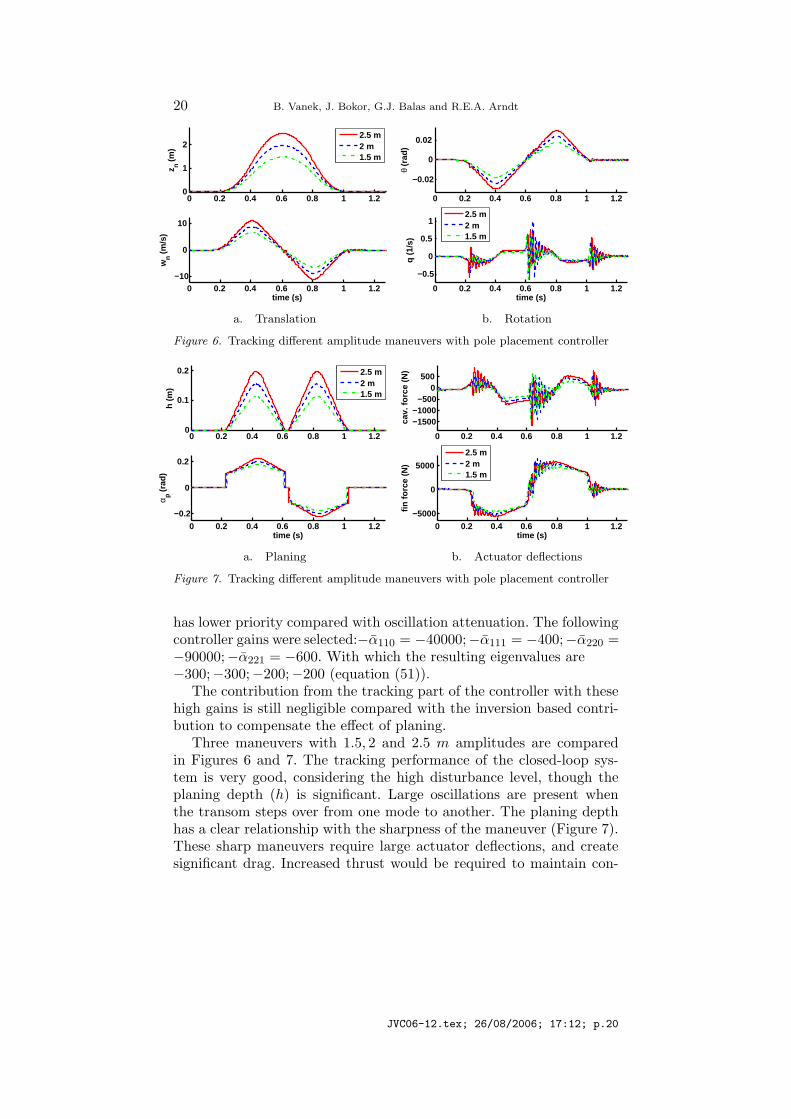
has lower priority compared with oscillation attenuation. The followingcontroller gains were selected:−α110 = −40000;−α111 = −400;−α220 =−90000;−α221 = −600. With which the resulting eigenvalues are−300;−300;−200;−200 (equation (51)).

The contribution from the tracking part of the controller with thesehigh gains is still negligible compared with the inversion based contri-bution to compensate the effect of planing.

Three maneuvers with 1.5, 2 and 2.5 m amplitudes are comparedin Figures 6 and 7. The tracking performance of the closed-loop sys-tem is very good, considering the high disturbance level, though theplaning depth (h) is significant. Large oscillations are present whenthe transom steps over from one mode to another. The planing depthhas a clear relationship with the sharpness of the maneuver (Figure 7).These sharp maneuvers require large actuator deflections, and createsignificant drag. Increased thrust would be required to maintain con-

JVC06-12.tex; 26/08/2006; 17:12; p.20


0 0.2 0.4 0.6 0.8 1 1.2

−0.5

0

0.5

1

time (s)

q (1

/s)

0 0.2 0.4 0.6 0.8 1 1.2−5000

0

5000

time (s)

fin fo

rce

(N) nom.

no act.

Figure 8. The actuator models role with pole placement controller

stant longitudinal speed. Including this additional control objective isundesirable, since thrust is not a control variable.

Accurate knowledge of delay in the cavity shape description playsan important role in the performance. The vehicle tracks the referencesignal well given accurate information of the delay. Imprecise knowledgeof the delay results in oscillations and the system becomes unstable atapproximate 15− 20% error. Simulations with 2.4 ms variation in thedelay lead to poor performance with oscillations and intensive actuatorusage.

The original controller was designed without an actuator model.The effect of a first order actuator with 30Hz bandwidth is consideredthrough the simulations. Significantly slower actuators were not ableto stabilize the system, while faster actuators achieved better perfor-mance. The case when the actuator is treated as unity (Figure 8) clearlyresults in better performance than the one with the first order actuatormodel, since only small oscillations occur. All other results presentedhave the actuator model included.

Sensitivity to cavity wall disturbances is investigated by varying themagnitude and frequency content of the disturbance. The maximumplaning depth remains the same if the disturbance magnitude increaseby a factor of 5 to 0.5 times the cavity gap, but the actuator deflectionsare slightly more aggressive. The response has larger spikes and haslonger settling times. Changing the second order disturbance filter to afirst or third order filter with the same bandwidth has a small effect onthe response. Hence the pole placement design is relatively insensitive

JVC06-12.tex; 26/08/2006; 17:12; p.21


to the smoothness of the cavity wall disturbance, because of the highplaning depth.

The vehicle has noticeably different dynamical behavior for longexcursion maneuver, which do not require high pitch rate motion,(Figure 12). The reference maneuver is a 4 s down-up maneuver withamplitude 20 m, and as suggested in (Dzielski and Kurdila, 2003) withthe reference on normal velocity (wref (t)) set to zero. The maneuvercan be executed without planing, because the disturbances on cavityshape fade away noticeably faster than the maneuver changes. Thecavity bubble is in quasi-steady state during the maneuver.

5.2. RHC simulation results

The continuous-time feedback linearization controller is implemented inthe inner-loop while the discrete RHC controller is running at 0.008 ssampling time as an outer-loop (Figure 5). The predictive controllerhas a six step prediction horizon, which is sufficiently longer than thedelay in the cavity description. The best results were achieved with athree step long control horizon, which allows sufficient freedom for thecontrol solutions but is less sensitive to uncertainties in the predictions.Constraints are chosen corresponding to the physical limitations of thevehicle. The maximum actuator deflections are set to ±0.2 rad andthe maximum deflection rates are ±100 rad/s. The maximum deflec-tion is meant to constrain the maximum achievable force, while itsangle value is less important, since the size of the fins are currentlyunder investigation. The maximum vertical speed is 28.75 m/s andthe maximum pitch angle is set to 0.25 rad to ensure the validityof small angle approximations. Structural loads are closely related tomaximum pitch rate which is constrained to ±10 rad/s. Drag reductionand smooth motion with extending the operation envelope of the vehiclecan be achieved with planing-free flight, while the control surface deflec-tions are also lower. The maximum transom deviation from the cavitycenterline is constrained to 1 cm, which is smaller than the nominalcavity gap (1.39 cm) to guarantee planing avoidance in the presence ofdisturbances.

The optimization problem weights differently the input and outputvariables. The input weight is set to 100 on both inputs, and theinput rate weight set to 50. These weights can be interpreted withthe knowledge of the output-error weights. The high position errorweight (25000) indicates that position tracking received the highestpriority, while the lower velocity error weight (1000), angle error weight(100) and angle rate error weight (2500) ensure that tracking of thesevariables have lower impact on the optimization. These slightly penal-

JVC06-12.tex; 26/08/2006; 17:12; p.22


0 0.2 0.4 0.6 0.8 1 1.20

1

2

z n (m

)

0 0.2 0.4 0.6 0.8 1 1.2−10

0

10

time (s)

wn (

m/s

)

2.5m2m1.5m

0 0.2 0.4 0.6 0.8 1 1.2

−0.1

0

0.1

θ (r

ad)

0 0.2 0.4 0.6 0.8 1 1.2

−0.5

0

0.5

1

time (s)

q (1

/s)

2.5m2m1.5m

a. Translation b. Rotation

Figure 9. Tracking different amplitude maneuvers with predictive controller

0 0.2 0.4 0.6 0.8 1 1.20

2

4

6x 10−4

h (m

)

0 0.2 0.4 0.6 0.8 1 1.2

−0.1

0

0.1

time (s)

α p (ra

d)

2.5m2m1.5m

0 0.2 0.4 0.6 0.8 1 1.2−600

−400

−2000

200

cav.

forc

e (N

)

0 0.2 0.4 0.6 0.8 1 1.2

−2000

200400600

time (s)

fin fo

rce

(N)

2.5m2m1.5m

a. Planing b. Actuator deflections

Figure 10. Tracking different amplitude maneuvers with predictive controller

ized variables improve stability with oscillation damping. The planingdepth is not weighted high (1000). It is important to note that theoutput variable constraints are implemented as soft constraints, andplaning depth constraint violations generate 10 times higher slack vari-able than other outputs. The slack variable weight is chosen to be2.5×109. The actuator model Gact = 200

s+200 , and the disturbance modelGn = 0.1

55.93(Rc−R) 106

s2+2000+106 are the same as before.The same 1.2 s reference trajectory on z(t), w(t), θ(t) and q(t) is

used. The results with the basic setup for 1.5, 2, and 2.5 m amplitudemaneuvers are shown in Figures 9 and 10.

The RHC reference tracking performance is less precise (Figure 12)than the pole placement controller, particularly on the signals withlower weights. The tradeoff is that planing occurs only for short periodswith low depth (Figure 10). Tracking is achieved with low actuator

JVC06-12.tex; 26/08/2006; 17:12; p.23


0 0.2 0.4 0.6 0.8 1 1.2

−0.5

0

0.5

q (1

/s)

0 0.2 0.4 0.6 0.8 1 1.2

−200

0

200

400

600

time (s)

fin fo

rce

(N) no act.

with act.

0 0.2 0.4 0.6 0.8 1 1.2−1

0

1

2

q (1

/s)

0 0.2 0.4 0.6 0.8 1 1.20

1

2

3

x 10−3

time (s)

h (m

)

high noisebasic

a. Actuator model b. Disturbance magnitude

Figure 11. Sensitivity of RHC tracking performance

deflections, without oscillations. As the trajectory becomes more ag-gressive, planing occurs more frequently. This requires increased actu-ator usage, though the maximum planing depth, unlike in the poleplacement case, is not increase with the trajectory amplitude. Theoverall control effort is significantly smaller than the pole placementdesign though at the expense of the state trajectories, especially theangle rate, being less smooth.

Uncertainty in delay time induces significant performance degra-dation because the bounds on constraining the maximum transomdeviation from the cavity centerline are very tight. Uncertainty inthe delay of 24 ms leads to oscillatory behavior, and larger controldeflections are commanded due to the consequent uncertainty in theplaning location. The closed-loop system becomes unstable around 10−15% (24− 36 ms) error in delay time.

The impact on tracking performance due to the addition of actu-ators, which are not addressed in the controller design, is shown inFigure 11. As one would expect, the performance is better if the actu-ator is perfect. Planing occurs for a very short time when actuatorsare included in the simulation. Assuming perfect actuators providereduced oscillations, at the expense of high-rate control signals, whatcan significantly influence the cavity stability (Syrstad et al., 2005).

The disturbance magnitude has a strong influence on the perfor-mance. A comparison with a disturbance magnitude of 0.1 and 0.5 cav-ity gap is shown in Figure 11. As the disturbance magnitude increases,planing occurs more frequently and the immersion depth increases.This leads to larger control deflections and fast angle rate responses.The position tracking performance is not significantly affected by thedisturbance level.

JVC06-12.tex; 26/08/2006; 17:12; p.24


0 0.2 0.4 0.6 0.8 1 1.20

1

2

z n (m

)

0 0.2 0.4 0.6 0.8 1 1.2−5000

0

5000

fin fo

rce

(N)

time (s)

P.P.RHC

0 1 2 3 4 5 6 70

10

20

z n (m

)

0 1 2 3 4 5 6 7−200

0

200

400

fin fo

rce

(N)

time (s)

P.P.RHC

a. 2 m maneuver b. 20 m maneuver

Figure 12. Comparison of pole placement and predictive controller

The bandwidth of the cavity disturbance model also influences theclosed-loop performance. Although limited information is available aboutthe cavity wall smoothness, it is natural to assume that it is not perfect.The selected disturbance magnitude is 0.1(Rc − R) passed through a1000 rad/s low-pass filter. The nominal simulation uses a second orderfilter Gnom(s) = 0.1

Knf(Rc−R) 106

s2+2000+106 which is normalized to provideapproximately maximum 0.1(Rc − R) magnitude signals. Two otherdisturbance filters are studied: a normalized first order (K1

1000s+1000) and

a third order one (K3109

s3+3000s2+3·106s+109 ), they are comparable in pointof all their poles are at 1000 rad/s and the maximum magnitude ofthe cavity disturbance is held constant. The closed-loop response withthird-order disturbance filter planes longer, also causing larger anglerates. Hence, it indicates the importance of correct characterization ofthe cavity wall disturbance.

Longer maneuvers with higher amplitude excursions (4 s, 20 m) arealso considered with the RHC design (Figure 12). As expected fromthe pole placement results, planing does not occur with the recedinghorizon approach. The state and control trajectories are very similarto the pole placement case. Figure 12 also shows the importance ofplaning avoidance, since the pole-placement controller commands unre-alistically high actuator deflections in the short maneuver when planingoccurs.

A simulation is performed with only a position reference signal,while all the other states are desired to be zero, to analyze how theconstraints restrict the motion of the vehicle. Slight degradation in theposition tracking performance is observed. The actuator deflection andall the vehicle state trajectories are very close to the original reference

JVC06-12.tex; 26/08/2006; 17:12; p.25


0 0.2 0.4 0.6 0.8 1 1.2

−0.5

0

0.5

q (1

/s)

0 0.2 0.4 0.6 0.8 1 1.2−0.2

0

0.2

0.4

time (s)

δ f (ra

d)

satur.non sat.

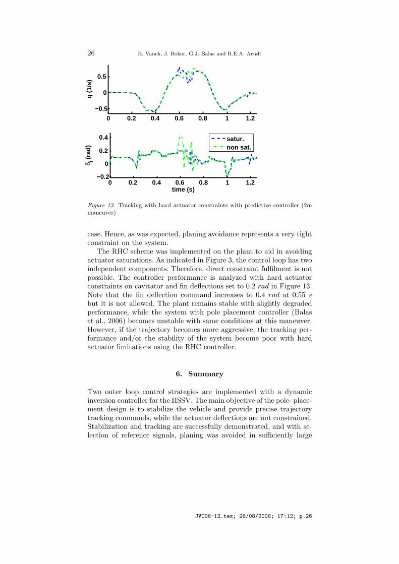
Figure 13. Tracking with hard actuator constraints with predictive controller (2mmaneuver)

case. Hence, as was expected, planing avoidance represents a very tightconstraint on the system.

The RHC scheme was implemented on the plant to aid in avoidingactuator saturations. As indicated in Figure 3, the control loop has twoindependent components. Therefore, direct constraint fulfilment is notpossible. The controller performance is analyzed with hard actuatorconstraints on cavitator and fin deflections set to 0.2 rad in Figure 13.Note that the fin deflection command increases to 0.4 rad at 0.55 sbut it is not allowed. The plant remains stable with slightly degradedperformance, while the system with pole placement controller (Balaset al., 2006) becomes unstable with same conditions at this maneuver.However, if the trajectory becomes more aggressive, the tracking per-formance and/or the stability of the system become poor with hardactuator limitations using the RHC controller.

6. Summary

Two outer loop control strategies are implemented with a dynamicinversion controller for the HSSV. The main objective of the pole- place-ment design is to stabilize the vehicle and provide precise trajectorytracking commands, while the actuator deflections are not constrained.Stabilization and tracking are successfully demonstrated, and with se-lection of reference signals, planing was avoided in sufficiently large

JVC06-12.tex; 26/08/2006; 17:12; p.26


maneuvers. The pole-placement controller was insensitive to cavitydisturbances, though the performance is strongly affected by the delaytime. For certain cases, the pole-placement controller led to signifi-cant immersion into the fluid requiring high actuator deflections whichresulted in increased drag on the hull and fins.

With the receding horizon approach, planing avoidance was suc-cessfully incorporated into the performance objectives at the expense ofreduced tracking precision and higher sensitivity to cavity disturbancesand delay information. The smaller immersion depth and actuator de-flections led to significantly lower drag in all maneuvers. Although theapproach relies heavily on the precision of the vehicle mathematicalmodel, its beneficial properties make it a reasonable method for furtherdevelopment.

7. Conclusion

Supercavitation is a very promising way to increase the speed of un-derwater vehicles at the expense of a complicated vehicle architecture.Successful development of such system will require increased collabora-tion between fluid and control researchers. As an intermediate step, thecontrol design challenges including delayed state dependency, nonlin-earities, and switching with disturbed switching surface were analyzed.An inversion based control methodology with RHC extension was pro-posed for the 2-DOF mathematical model of the HSSV. An extensivecomparison was made between a classical linear outer-loop controllerand the receding horizon controller. The objective of planing avoid-ance was solved, for a limited operating range. Important aspects ofthe reference maneuvers were analyzed and sensitivity properties (avulnerable point of dynamic inversion) were studied with respect todifferent cavity disturbances.

The next step of the analysis is to study the use of a single actuatorfor control (cavitator or fins), to understand the system tradeoffs. Theultimate goal remains the implementation of a three dimensional tra-jectory tracking controller on the HSSV test vehicle. It is likely that thecontroller for the high fidelity supercavitating model would require again-scheduled controller. This raises interesting issues with the designof dynamic inversion controller as the model parameters, like velocityor fin immersion, vary.

Furthermore, robust constraint fulfillment remains an open issue,which can be attempted to solve by further developments on the pro-posed receding horizon control based method.

JVC06-12.tex; 26/08/2006; 17:12; p.27


8. Acknowledgments

This work was funded by the Office of Naval Research, award numberN000140110229, Dr. Kam Ng Program Manager.

References

Arndt, R., G. Balas, and M. Wosnik: 2005, ‘Control of cavitating flows: A per-spective’. Japan Society of Mechanical Engineers International Journal, 48(2):334-341.

Ashley, S.: 2001, ‘Warp drive underwater’. Scientific American, 42–51.Balas, G., J. Bokor, B. Vanek, and R. Arndt: 2006, Control of Uncertain Systems:

Modelling, Approximation and Design, Chapt. Control of High-Speed Under-water Vehicles, pp. 25–44, Lecture Notes in Control and Information Sciences.Springer-Verlag.

Balas, G., R. Chiang, A. Packard, and M. Safanov: 2005a, ‘Robust Control Toolbox’.MUSYN Inc. and The MathWorks, Natick MA.

Balas, G. J., Z. Szabo, and J. Bokor: 2005b, ‘Controllability of bimodal LTI systems’.submitted to: IEEE Transactions on Automatic Control.

Bemporad, A., M. Morari, and N. Ricker: 2005, Model Predictive Control ToolboxUser’s Guide. The Mathworks.

Camlibel, M., W. Heemels, and J. Schumacher: 2004, ‘On the controllability ofbimodal piecewise linear systems’. In:Alur R, Pappas GJ (eds.) Hybrid Systems:Computationand Control LNCS 2993, Springer, Berlin, 250–264.

DARPA Advanced Technology Office: 2005, ‘Underwater Express’. In: BAA06-13Proposer Information Pamphlet (PIP).

Doyle, J., K. Glover, P. Khargonekar, and B. Francis: 1989, ‘State-space solutions tostandard H2 and H∞ control problems’. IEEE Trans Auto Control 34:831–847.

Dzielski, J. and A. Kurdila: 2003, ‘A Benchmark Control Problem for Supercavitat-ing Vehicles and an Initial Investigation of Solutions’. Journal of Vibration andControl 9(7), 791–804.

Goel, A.: 2002, ‘Control Strategies for Supercavitating Vehicles’. Master’s thesis,University of Florida.

Kirschner, I., D. Kring, A. Stokes, and J. Uhlman: 2002a, ‘Control strategies forsupercavitating vehicles’. J Vibration and Control 8:219–242.

Kirschner, I., B. J. Rosenthal, and J. Uhlman: 2003, ‘Simplified Dynamical Sys-tems Analysis of Supercavitating High-Speed Bodies’. In: Fifth InternationalSymposium on Cavitation (CAV2003). Osaka,Japan.

Kirschner, I. N., D. C. Kring, A. W. Stokes, N. E. Fine, and j. James S. Uhlman:2002b, ‘Control Strategies for Supercavitating Vehicles’. Journal of Vibrationand Control 8, 219–242.

Kurdila, A. J., R. Lind, J. Dzielski, A. Jammulamadaka, and A. Goel: 2003, ‘Dynam-ics and Control of Supercavitating Vehicles’. Technical report, Office of NavalResearch Supercavitating High Speed Bodies Workshop.

Lin, G., B. Rosenthal, E. Abed, and B. Balachandran: 2004, ‘Dynamics and Controlof Supercavitating Bodies’. In: TECH2004.

Logvinovich, G.: 1972, ‘Hydrodynamics of free-boundary flows’. translated from theRussian (NASA-TT-F-658), US Department of Commerce, Washington D.C.

Maciejowski, J.: 2002, Predictive Control with Constraints. Prentice Hall.

JVC06-12.tex; 26/08/2006; 17:12; p.28


Mayne, D., J. Rawlings, C. Rao, and P. Scokaert: 2000, ‘Constrained modelpredictive control: stability and optimality’. Automatica (36), 789–814.

McFarlane, D. and K. Glover: 1992, ‘A Loop Shaping Design Procedure using H∞Synthesis’. IEEE Trans Auto Control 37:759–769.

Safonov, M.: 1987, Modelling, Robustness and Sensitivity Reduction in ControlSystems, Chapt. Imaginary-axis zeros in H∞ optimal control, pp. 71–82.Springer-Verlag.

Shao, Y., M. Mesbahi, and G. Balas: 2003, ‘Planing, switching and supercavitatingflight control’. AIAA Guidance, Navigation and Control Conference, AIAA-2003-5724.

Syrstad, J., M. Wosnik, G. Balas, and R. E. Arndt: 2005, ‘Control of a Supercavity-Piercing Fin’. In: 58th Annual Meeting of the Division of Fluid Dynamics.

Vanek, B., J. Bokor, and G. J. Balas: 2006a, ‘High-Speed Underwater VehicleControl’. AIAA Guidance, Navigation, and Control Conference, Keystone.

Vanek, B., J. Bokor, and G. J. Balas: 2006b, ‘Theoretical aspects of High-SpeedUnderwater Vehicle Control’. American Control Conference, Minneapolis.

Vasin, A. and E. Paryshev: 2001, ‘Immersion of a Cylinder in a Fluid Througha Cylindrical Free Surface’. Fluid Dynamics 36(2), 169–177. translated fromRussian.

JVC06-12.tex; 26/08/2006; 17:12; p.29

Longitudinal Motion Control of a High-Speed ... · Longitudinal Motion Control of a High-Speed...

Documents

Transcript of Longitudinal Motion Control of a High-Speed ... · Longitudinal Motion Control of a High-Speed...