Long-wavelength surface-tension-driven Benard …chaos.ph.utexas.edu/manuscripts/1081888161.pdf ·...

J. Fluid Mech. (1997), vol. 345, pp. 45–78. Printed in the United Kingdom

c© 1997 Cambridge University Press

45

Long-wavelength surface-tension-driven Benardconvection: experiment and theory

By S T E P H E N J. V A N H O O K, M I C H A E L F. S C H A T Z†,J. B. S W I F T, W. D. M C C O R M I C K,

AND H A R R Y L. S W I N N E Y

Center for Nonlinear Dynamics and Department of Physics,University of Texas at Austin, Austin, TX 78712, USA

e-mail: [email protected]

(Received 30 September 1996 and in revised form 4 March 1997)

Surface-tension-driven Benard (Marangoni) convection in liquid layers heated frombelow can exhibit a long-wavelength primary instability that differs from the morefamiliar hexagonal instability associated with Benard. This long-wavelength instabilityis predicted to be significant in microgravity and for thin liquid layers. The instabilityis studied experimentally in terrestrial gravity for silicone oil layers 0.007 to 0.027 cmthick on a conducting plate. For shallow liquid depths (< 0.017 cm for 0.102cm2 s−1 viscosity liquid), the system evolves to a strongly deformed long-wavelengthstate which can take the form of a localized depression (‘dry spot’) or a localizedelevation (‘high spot’), depending on the thickness and thermal conductivity of thegas layer above the liquid. For slightly thicker liquid depths (0.017–0.024 cm),the formation of a dry spot induces the formation of hexagons. For even thickerliquid depths (> 0.024 cm), the system forms only the hexagonal convection cells.A two-layer nonlinear theory is developed to account properly for the effect ofdeformation on the interface temperature profile. Experimental results for the long-wavelength instability are compared to our two-layer theory and to a one-layertheory that accounts for the upper gas layer solely with a heat transfer coefficient.The two-layer model better describes the onset of instability and also predicts theformation of localized elevations, which the one-layer model does not predict. Aweakly nonlinear analysis shows that the bifurcation is subcritical. Solving for steadystates of the system shows that the subcritical pitchfork bifurcation curve never turnsover to a stable branch. Numerical simulations also predict a subcritical instabilityand yield long-wavelength states that qualitatively agree with the experiments. Theobservations agree with the onset prediction of the two-layer model, except for verythin liquid layers; this deviation from theory may arise from small non-uniformitiesin the experiment. Theoretical analysis shows that a small non-uniformity in heatingproduces a large steady-state deformation (seen in the experiment) that becomesmore pronounced with increasing temperature difference across the liquid. Thissteady-state deformation becomes unstable to the long-wavelength instability at asmaller temperature difference than that at which the undeformed state becomesunstable in the absence of non-uniformity.

† Present address: School of Physics, Georgia Institute of Technology, Atlanta, GA 30332, USA.

46 S. VanHook, M. Schatz, J. Swift, W. McCormick and H. Swinney

1. Introduction

Surface-tension-driven phenomena are important not only for their influence onthe fundamental physics of interfacial flows, but also for their potential industrialapplications, particularly in microgravity where buoyancy effects nearly disappear. Inthe presence of temperature variations on a liquid–fluid interface, the temperaturedependence of surface tension (dσ/dT ≡ −σT < 0) causes cool regions of theinterface to pull liquid from warm regions of the interface. This thermocapillarymechanism can drive fluid flow and lead to instabilities in non-isothermal free-surfacesystems (Davis 1987). In surface-tension-driven Benard convection (henceforth called‘Marangoni convection’), a liquid layer is heated from below and cooled from above(see figure 1). In thin liquid layers or in microgravity, the buoyancy mechanismof Rayleigh–Benard convection becomes negligible, leaving thermocapillarity as thedominant driving mechanism (Davis & Homsy 1980).

Benard (1900) performed some of the earliest studies of convection in liquid layersalmost a century ago. Heating thin layers (≈ 1 mm deep) of spermaceti from below, hefound a transition from conduction to polygonal (quasi-hexagonal) convection cells ofwavenumber q ≡ 2πd/λ ≈ 2, where d is the mean liquid depth and λ is the wavelengthof the cells. Block (1956) and Pearson (1958) first recognized that surface tension, notbuoyancy, was the source of the instability. Benard’s experiments have been repeated(Koschmieder & Biggerstaff 1986) and the most recent experiment by Schatz et al.(1995) found onset of the instability in close agreement with the prediction of linearstability analysis (Pearson 1958; Nield 1964). In addition, Schatz et al. found that thebifurcation was subcritical with 3.2% hysteresis, larger than predicted by nonlineartheory (Scanlon & Segel 1967, 2.3%; Cloot & Lebon 1984, 0.2%).

A second and completely different instability due to surface tension also existsin this same system and should become primary in very thin or very viscous liquidlayers or in microgravity. This long-wavelength (q = 0) deformational mode was firstpredicted thirty years ago by Scriven & Sternling (1964) and Smith (1966) and hasrecently been observed experimentally by VanHook et al. (1995). In the experiments,a thin liquid layer heated from below became unstable and eventually formed alarge-scale drained region (‘dry spot’). The experiments found onset of the instabilityto occur 35% below the prediction of linear stability analysis of a one-layer model(Takashima 1981a; Goussis & Kelly 1990; Perez-Garcıa & Carneiro 1991; Wilson1993).

Another long-wavelength instability, unrelated to the one described in the previousparagraph, was predicted by Pearson (1958) and further discussed by Sivashinsky(1982), Garcia-Ybarra, Castillo & Velarde (1987), and Hadji, Safar, & Schell (1991)for perfectly insulating top and bottom boundaries. Since this instability is predictedto occur for even a non-deformable interface, it is fundamentally different from thelong-wavelength instability that is the subject of this paper. Pantaloni et al. (1979)claimed to observe the long-wavelength mode of Pearson in silicone oil on top of aglass plate; however, it is clear they did not observe this state because the bottomboundary condition was conducting relative to the liquid (kglass/k ≈ 6). Takashima(1970) generalized Pearson’s analysis to finite kbottom/k and predicted little differencebetween the case of an infinitely conducting bottom and kbottom/k = 6; in addition, forkbottom/k even as small as 0.1, he predicts a finite wavelength (q ≈ 1). Observation ofthe long-wavelength mode with insulating boundaries would require kbottom/k < 0.01and d/dg 1. Even styrofoam has too large a thermal conductivity by an order ofmagnitude.

Long-wavelength Marangoni convection 47

Cooled sapphire window

Heated metal mirror

Tt

Tb

Gas

LiquidWarm

Cool¡r

h (x, y, t)

dg

dgz

L

Figure 1. Sketch of a surface-tension-driven Benard (Marangoni) convection cell of horizontalextent L, mean liquid depth d, mean gas depth dg , and local interface position h(x, y, t). In allexperiments L/d > 100, and dg is typically twice d. The sapphire window is cooled to temperatureTt and the mirror is heated to temperature Tb. Since surface tension decreases with increasedtemperature, temperature variations generate surface tension gradients, which can initiate fluid flow.

Parameter Symbol Value at 50 C

Surface tension σ 19 dyn cm−1

Surface-tension coefficient σT 0.069 dyn cm−1 K−1

Liquid density ρ 0.94 g cm−3

Liquid thermal diffusivity κ 0.001 cm2 s−1

Liquid kinematic viscosity ν 0.102 cm2 s−1

Liquid thermal expansion α 0.001 C−1

Liquid thermal conductivity k 13.3 × 103 erg s−1 cm−1 K−1

Gas thermal conductivity kg 2.76 × 103 erg s−1 cm−1 K−1 (air)15.3 × 103 erg s−1 cm−1 K−1 (He)

Table 1. Fluid parameter values

The hexagonal and long-wavelength instabilities differ in the stabilizing mecha-nisms that compete with destabilizing thermocapillary effects due to different types offluctuations. The short-wavelength hexagonal instability originates from temperaturefluctuations on the free surface, which initiate thermocapillary flow along the inter-face; the imposed vertical temperature difference across the liquid layer sustains theflow. Thermal and viscous diffusion, however, dampen the temperature fluctuationsand associated fluid flow. Alternatively, the long-wavelength mode originates fromfluctuations of the free-surface height h(x, y), which cause a temperature variation onthe interface because of the imposed temperature gradient. By thermocapillarity, thecool elevated region pulls liquid from the warm depressed region and, if allowed tocontinue, thermocapillarity would pile all the liquid from one region of the layer intoan adjacent region. Gravity, though, attempts to flatten the interface and thus tostabilize these deformational perturbations. In addition, surface tension selects a longwavelength for this deformational instability since surface tension resists curvature ofthe interface and thus stabilizes long-wavelength modes least.

The onset behaviour of the system is determined by three time scales – thermo-capillary (t2therm = ρd3/σT∆T ), gravitational (t2grav = d/g), and diffusive (t2diff = d4/νκ),where g is the gravitational acceleration, ∆T is a characteristic temperature differenceacross the liquid layer, and other parameters are defined in figure 1 and table 1.Thermocapillarity is destabilizing, while gravity and diffusion are stabilizing. TheGalileo number,

G ≡t2diff

t2grav=gd3

νκ, (1.1)


(a) (b)300

200

100

M

300

200

100

M G23

G23

0 1 2 3 4 0 1 2 3 4q q

Figure 2. Marginal stability curves for ν = 0.10 cm2 s−1 silicone oil in terrestrial gravity accordingto linear stability theory for d/dg 1 (see, for example, Smith 1966). (a) For d = 0.03 cm, theprimary instability appears at M = 80 with q = 1.99. (b) For d = 0.02 cm, the minimum at q = 0becomes the global minimum and the primary instability occurs at q = 0 and M = 2G/3 = 52.

determines which instability will appear – the stabilizing mechanism with the longesttime scale (i.e. the slowest-acting stabilizing mechanism) determines the criterion foronset.

When G is sufficiently large, the response time of gravity is short enough thatdeformational perturbations are quickly stabilized. The liquid surface can be con-sidered effectively flat and the formation of short-wavelength (hexagonal) convectioncells due to temperature perturbations is the primary instability (see figure 2a). Therelevant parameter for determining stability in this case is the Marangoni number, or

M ≡t2diff

t2therm=σT∆Td

ρνκ. (1.2)

When M > 80 (Pearson 1958), thermocapillarity is strong enough to overcomediffusion and onset of short-wavelength convection occurs.

When G is small, the diffusive time scale is very short, temperature perturbationsare quickly damped, and gravity is relatively weak so that deformational pertur-bations which generate the long-wavelength instability are slowly stabilized. Thelong-wavelength instability becomes primary (see figure 2b) and the relevant param-eter for determining onset of the instability is the inverse dynamic Bond number,

D ≡t2grav

t2therm=M

G=σT∆T

ρgd2. (1.3)

When D >≈ 2/3 (Smith 1966), the thermocapillary effect is strong enough to overcomegravity and the system is unstable to long-wavelength deformations.

When both liquid and gas layers are conducting and the interface is not deformed,the uniform temperature difference across the liquid layer ∆T can be calculated fromthe top Tt and bottom Tb temperatures,

∆T =Tb − Tt

1 + dgk/dkg=

(Tb − Tt)H1 +H

, (1.4)

where H = dkg/dgk. The long-wavelength instability is a deformational mode,however, and in the presence of deformation the temperature field is no longerhorizontally uniform. For small deformation, the mean temperature difference acrossthe layer 〈∆T 〉 is still given by (1.4). For large deformation, however, (1.4) does


Dimensionless number Symbol Definition Typical values

Galileo G gd3/νκ 0–150Marangoni M σT∆Td/ρνκ 0–100Inverse dynamic bond D σT∆T/ρgd2 0–0.7Rayleigh R αg∆Td3/νκ 0–1Static Bond B ρg(L/2π)2/σ 18Biot H kgd/kdg 0–1Two-layer Biot F (d/dg −H)/(1 +H) −0.1–1.0Crispation Cr ρνκ/σd 10−4–10−3

Prandtl Pr ν/κ 100

Table 2. Dimensionless quantities and experimental values

not give 〈∆T 〉 (see §4); the difference between ∆T as defined in (1.4) and 〈∆T 〉 ismodel-dependent, but for either the one- or two-layer models, ∆T differs from 〈∆T 〉by only a few percent for moderate deformation. Using 〈∆T 〉 as the characteristictemperature drop across the liquid is problematic since then D would increase whenthe instability occurs and the interface begins to deform, even for fixed Tb and Tt.We use ∆T as defined by (1.4) as the characteristic temperature difference acrossthe liquid for both theory and experiment; thus there is no problem in comparingexperiment to theory.

Marangoni convection has been described by both one-layer and two-layer models.One-layer models explicitly model the liquid layer and model the upper gas layersolely with a heat transfer coeffiecient (the Biot number). Two-layer models explicitlymodel both liquid and gas layers. In this paper, we employ a two-layer model thattakes into account the conduction heat transfer in the gas layer in the presence ofdeformation, but ignores convection in the gas layer.

Section 2 discusses the one-layer model which has been employed in most theoret-ical work on the Marangoni problem. Section 3 begins by explaining the necessity ofusing a two-layer model for the long-wavelength instability and the remainder of §3develops a two-layer nonlinear theory for the long-wavelength mode. Section 3.1 de-rives a nonlinear evolution equation to describe the instability; §3.2 performs a linearanalysis of the evolution equation; §3.3 performs a weakly nonlinear analysis to deter-mine the nature of the bifurcation; §3.4 solves for steady states for a one-dimensionalinterface (rolls); §3.5 discusses numerical simulations of the evolution equation. Sec-tion 3.6 discusses the effect of non-uniformity in the system. Section 4 describes theexperimental design and §5 presents the experimental results. Conclusions are givenin §6.

2. One-layer modelMost linear stability analyses of the Marangoni problem (Pearson 1958; Nield

1964; Takashima 1981a; Goussis & Kelly 1990; Perez-Garcıa & Carneiro 1991;Wilson 1993) have employed a one-layer model, where the effect of the gas in theupper layer is modelled solely by a heat transfer coefficient, the Biot number, whichfor a flat interface is

H(q) = qkg

kcoth q

dg

d(2.1)


(see, for example, equation 8.91 of Cross & Hohenberg 1993 or the appendix ofHadji et al. 1991). As q → 0, H → kgd/kdg (for the remainder of the paper, H willmean H(q → 0)). The earliest linear stability analyses assumed a non-deformableinterface (Pearson 1958; Nield 1964) and thus never discovered the inherently de-formational long-wavelength mode. Scriven & Sternling (1964) first predicted thislong-wavelength instability, which they found marginally stable at M = 0. Thus, ac-cording to their analysis, this q = 0 mode should always appear before the hexagonsand, in fact, appear with infinitesimal ∆T . Smith (1966) pointed out that their analysisignored gravity, which induces hydrostatic pressure differences that resist deformation.Depending on the strength of gravity, either the hexagonal or the long-wavelengthmode could appear as the primary instability. Later linear stability analyses employ-ing a one-layer model that allowed for deformation (Takashima 1981a; Goussis &Kelly 1990; Perez-Garcıa & Carneiro 1991) predicted onset of the q = 0 mode at

Dc = 23(1 +H). (2.2)

These results are for an infinite system. A finite system of horizontal extent L has alowest-order mode of q = 2πd/L, which should become unstable at a slightly higher(∼ O(q2)) value of D.

While the one-layer linear stability theory successfully predicts the onset of theq = 1.99 Pearson/Benard instability, it is less successful with the long-wavelengthinstability. The only experiment to test this theory (VanHook et al. 1995) found thatthe onset in the experiments occurs 35% earlier than predicted by the one-layer lineartheory.

A one-layer model nonlinear evolution equation for the long-wavelength instabilitywas derived by Davis (1983) for H = 0. A slightly different equation was derivedby Funada (1987), and the extension to finite H was derived by Kopbosynov &Pukhnachev (1986) and Oron & Rosenau (1992). A linear stability analysis basedon this equation agrees with (2.2). Numerical simulations of the equation find theformation of a large-scale dry spot (Joo, Davis & Bankoff 1991; VanHook et al.1995; Krishnamoorthy & Ramaswamy 1995), in qualitative accord with what is seenin experiments (VanHook et al. 1995).

3. Two-layer modelA thermocapillary model with two fluid layers was first considered by Smith (1966).

He found a negligible correction (of order 1% for most parameters) to the one-layerprediction for the onset of hexagons (q = 2), but found onset of the long-wavelengthmode (q = 0) at

Dc =2(1 +H)

3(1 + d/dg)=

2

3(1 + F)(3.1)

(equation (28) in his paper), where the new parameter, which we call the two-layerBiot number,

F ≡ d/dg −H1 +H

, (3.2)

replaces H as the relevant heat transfer coefficient. Nepomnyashchii & Simanovskii(1990) and Golovin, Nepomnyashchy & Pismen (1997) revisited the two-layer modeland found the same linear instability onset. This two-layer prediction (3.1) agreesbetter with experiment (see §5) than the onset predicted by the one-layer model (2.2).


nz

tiˆ

x⊥iˆ

Gas

Liquid h (x, y, t)

Figure 3. Sketch defining directions. x⊥,i ≡ (x, y) and z are Cartesian coordinates defined globally.

The directions n and ti are, respectively, the directions normal and tangent to the surface (the twotangent directions are indexed by i).

We introduce here a two-layer nonlinear model that gives better agreement withexperiment than does the one-layer model and correctly predicts the formation oflocalized elevations (‘high spots’), as well as localized depressions (‘dry spots’). Thetwo-layer model takes into account the full effect of the deformation upon the surfacetemperature profile. In the one-layer model, an elevated region of the interface iscooler because it is farther from the heater; in the two-layer model, an elevated regionof the interface is even cooler (than in the one-layer model) because the elevated regionis also closer to the cool upper plate. That is, the two-layer model also takes intoaccount the decrease in the thickness of the gas layer between the interface and thetop plate, thus increasing the effect of the deformation. This additional effect increasesin influence with increasing d/dg .

3.1. Nonlinear evolution equation

In this section we derive a nonlinear evolution equation which encompasses both theone- and two-layer models. The two-layer model equation predicts the existence of anew state, a localized elevation, which is not predicted by the one-layer model. Figure3 shows the notation.

We take the local interface temperature to be given by (1.4) with d → dh(x, y, t)and dg/d→ [dg/d− (h(x, y, t)− 1)], or

T (x, y, z = h) = Tb −Tb − Tt

1 +(dg/d− h(x, y, t) + 1)k

h(x, y, t)kg

= Tb −∆T h

1 + F − Fh, (3.3)

where h(x, y, t) is non-dimensionalized by d. (The one-layer model fails to include thechange in the local air depth due to variations in h; thus in the limit of d/dg → 0, wheresuch variations would be negligible, the one- and two-layer predictions coincide.) This‘reduced’ model assumes pure conduction in both liquid and gas layers, requires alldisturbances to have a long wavelength so that thermal diffusion in the horizontaldirections can be neglected, and ignores any viscous coupling or driven thermalconvection in the upper (gas) layer. We ignore these effects in order to isolatethe aspect of the full two-layer theory necessary to capture the phenomena. (Forq 1, there is no difference between this reduced theory and the full linear theory.)Temperature variations not due to deformational perturbations are ignored since G isassumed small enough that the diffusive timescale is much faster than the gravitationaltimescale.


The relevant equations for this system are, respectively, Navier–Stokes, tempera-ture, continuity, velocity and temperature boundary conditions at the bottom plate,kinematic boundary condition, tangential and normal stress boundary conditions atthe interface, and the temperature boundary condition at the top plate:

1

Pr

[∂u

∂t+ (u · ∇)u

]= −∇P + ∇2u− Gz, (3.4a)

∂T

∂t+ (u · ∇)T = ∇2T , (3.4b)

∇ · u = 0, (3.4c)

T = u = 0 at z = 0, (3.4d)

w =∂h

∂t+ u · ∇h at z = h, (3.4e)

∂S

∂xti=

(∂un

∂xti+∂uti∂xn

)(i = 1, 2) at z = h, (3.4f)

P − S(

1

R1

+1

R2

)= 2

(∂un

∂xn

)at z = h, (3.4g)

T = −1 +H

Hat z = 1 +

dg

d. (3.4h)

R1 and R2 are the local radii of curvature of the interface. We separate the velocityinto horizontal (u⊥) and vertical (w) components. In addition,

∇⊥ ≡ x∂

∂x+ y

∂

∂y.

Since h(x, y) does not depend on z, ∇h = ∇⊥h. All lengths are scaled by d, timeby d2/κ, velocities by κ/d, pressure by ρνκ/d2, temperatures by ∆T , and surfacetension by ρνκ/d. In the absence of deformation, the dimensionless surface tensionis S ≡ σd/ρνκ = Cr−1, where Cr is the Crispation number. The dimensionlessgravitational acceleration is G, the Galileo number. The temperature derivative ofsurface tension is non-dimensionalized so that −∂S/∂T ≡ M (the liquid is assumedBoussinesq, which is a good approximation in our experiments). The height of theinterface h(x, y) is non-dimensionalized by the mean liquid depth d, so h(x, y) = 1 isthe undeformed state. We assume that the change in surface tension is small, or

σT∆T

σ= MCr 1. (3.5)

We follow the method used by Davis (1983) and expand the equations of motionin terms of the magnitude of the fundamental wavevector q (= 2πd/L), which isassumed to be small (d L). All time derivatives and spatial derivatives in thehorizontal direction are taken to be of order q; derivatives in the vertical directionare of O(1). Equation (3.4c) then requires that w is one order higher in q than u⊥.We adopt the following scalings: u⊥ ∼ O(1), w ∼ O(q), and P ∼ O(q−1). In addition,S must be of O(q−3), ∂S/∂T ∼ O(q−1), G ∼ O(q−1), and Pr > O(1). These scalingsare necessary in order that the three important effects (thermocapillarity, gravity, and


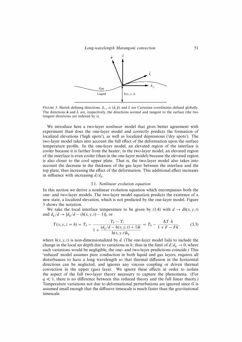
surface tension) appear at lowest order. The lowest-order equations are

∂2u⊥

∂z2= ∇⊥P ,

∂P

∂z+ G = 0,

∂2T

∂z2= 0, (3.6a–c)

∇⊥ · u⊥ +∂w

∂z= 0, (3.6d)

T = u⊥ = w = 0 at z = 0, (3.6e)

∂h

∂t= w − u⊥ · ∇h at z = h, (3.6f)

∇h · ∇S + (∇h · ∇h)∂T∂z

(dS

dT

)− ∇h · ∂u⊥

∂z= 0 at z = h, (3.6g)[

∇h× ∇⊥S − ∇h×∂u⊥∂z

]· z = 0 at z = h, (3.6h)

P + S∇2h = 0 at z = h, T =−h

1 + F − Fh at z = h (3.6i, j)

In determining the interfacial temperature profile (3.6j), we used (3.6c), which impliesthat the temperature profile is purely conductive and that diffusion in the horizontaldirection is negligible, and thus (3.3) is a valid approximation. From (3.6b) and (3.6i),we have

P (x, t) = −S∇2h+ G(h− z). (3.7)

From (3.6a), we have

∂2u⊥

∂z2= −S∇∇2h+ G∇h. (3.8)

Integrating over z twice and applying (3.6e), we have

u⊥ = (−S∇∇2h+ G∇h) 12z2 + a(x⊥, t)z. (3.9)

Using (3.6g) to find a, we have

u⊥ =(−S∇∇2h+ G∇h

)12z2 + z

(Sh∇∇2h− Gh∇h+ ∇S

). (3.10)

Using (3.6d) and (3.6e), we solve for the vertical velocity:

w = (S∇2∇2h− G∇2h) 16z3 − 1

2z2[S∇ ·

(h∇∇2h

)− G∇ · (h∇h) + ∇2S

]. (3.11)

Using (3.6f), we obtain ∂h/∂t. We rescale the domain of both x and y to [0,2π), sothat the wavevectors q become integers. In addition, time is rescaled by G(L/2πd)2/3to G(L/2π)2/3κ. The final two-dimensional evolution equation for the local liquiddepth h(x, y, t) is then

∂h

∂t+ ∇ ·

3D

2

(1 + F)h2∇h(1 + F − Fh)2

− h3∇h+h3

B∇2∇h

= 0, (3.12)

where F is given by (3.2), D is the inverse dynamic Bond number given by (1.3), andB is the static Bond number, B ≡ ρg(L/2π)2/σ > 0. The first term in curly bracketsdescribes the effect of thermocapillarity; the second, gravity; and the third, surfacetension.

The equation of Davis (1983, 1987) is recovered for F = 0; the one-layer modelequation (Kopbosynov & Pukhnachev 1986; Oron & Rosenau 1992; Deissler & Oron


cq

(a) ε!0 (b) ε"0

0 1 2q

0 1 2q

0

–0.5

0

–0.5

q2max=Bε

Figure 4. Growth rates γq as a function of q for (a) ε negative (ε = −0.01) and (b) ε positive(ε = 0.1) according to linear, long-wavelength theory (B = 30).

1992) is recovered for d/dg → 0, i.e. F = −H/(1 + H); thus the one-layer equationalways has F 6 0, while F can be (and usually is) positive in the two-layer model.In both one- and two-layer models, F > −1. For F > 0, there is a restriction thath(x, y) < (1 + dg/d) < (1 + F)/F . Also, the fluid cannot penetrate the bottom plate,or h(x, y) > 0. (This is enforced in the equation by ∂h/∂t = 0 if h = 0.)

Equation (3.12) is fourth order and thus needs four boundary conditions. Two canbe obtained by assuming that the sidewalls pin the meniscus of the liquid, or

h(0) = h(2π) = 1.

However, there is no clear choice for the second pair of boundary conditions. For therest of this paper, we will use periodic boundary conditions, which greatly simplifythe analysis.

3.2. Linear analysis

The linearization of (3.12) is

∂h

∂t+ ε∇2h+

1

B∇2∇2h = 0, (3.13)

where

ε ≡ M(1 + F)− 2G/3

2G/3=

3D(1 + F)

2− 1. (3.14)

Assuming a linear solution h = 1 + ηq1 ,q2eγqtei(q1x+q2y), one obtains the growth rate of

the qth mode (q2 = q21 + q2

2),

γq = q2(ε− q2/B

)≡ q2εq, (3.15)

where εq is the control parameter appropriate for a mode of finite wavenumber q.Since modes with q > 0 begin to become unstable for ε > 0 (see figure 4), the linearstability analysis of (3.12) agrees with the two-layer linear stability analysis of the fullequations (3.1) for q = 0.

The linear stability analyses of Takashima (1981b) and Perez-Garcıa & Carneiro(1991) predict the existence of an oscillatory instability for M < 0. For PrCr 10−3,Takashima (1981b) predicts that this oscillatory instability will appear with a longwavelength. Since only even derivatives of q appear in (3.13), (3.12) does notcontain any oscillatory instabilities (complex γq). The frequency of an oscillatorymode would have to be small (∼ q) for the assumption of slow time scale madein the derivation to be correct. However, the long-wavelength oscillatory instability


0.05

0

–0.05–0.010 –0.005 0 0.005

ε1

Rolls

Squares

g

gr, sq= 0 –ε1

gr, sq1

1/2

Figure 5. Predicted subcritical bifurcation of the long-wavelength mode according to weaklynonlinear analysis (F = 0, B = 30) for both rolls and squares. Solid lines correspond to linearlystable states; dotted lines to linearly unstable states.

predicted by Takashima (1981b) and Perez-Garcıa & Carneiro (1991) has a fast (notO(q)) frequency and so cannot be described by (3.12).

3.3. Weakly nonlinear analysis

To determine the nature of the bifurcation, we performed a weakly nonlinear analysisof the evolution equation by considering just the two lowest-order wavenumbers inthe deformation:

h = 1 + (η10eix + η01e

iy + η11ei(x+y) + η1−1e

i(x−y) + η20e2ix + η02e

2iy) + c.c. (3.16)

We are interested in when the lowest-order finite mode (q = 1) becomes unstable,so we use

ε1 = ε− 1/B (3.17)

as our bifurcation parameter. We assume that (η10, η01) ∼ O(|ε1|1/2) and (η11, η1−1,η20, η02) ∼ O(|ε1|). Inserting the above expression for h(x, y) into the evolution equa-tion, keeping only the lowest-order terms and matching arguments of the exponentials,we find that

ε1η10 = −η10

[gr|η10|2 + (gsq − gr)|η01|2

], (3.18a)

ε1η01 = −η01

[gr|η01|2 + (gsq − gr)|η10|2

], (3.18b)

where

gr =B + 1

6B[(B + 7)− 4F(B + 4) + 2F2(2B + 11)], (3.19a)

gsq =B + 1

6B[(13B + 31)− 4F(13B + 22) + 2F2(26B + 53)]. (3.19b)

The two solutions of this equation are rolls (η ≡ η10, η01 = 0, or vice versa) andsquares (η ≡ |η10| = |η01|). For all values of F and B (> 0), gsq > gr > 0; thus thebifurcation is predicted to be a subcritical pitchfork for both rolls and squares (seefigure 5), with the squares branch always closer to the axis than the rolls branch.Since gr and gsq have their minimum at F = 1/2 for B > 10, the unstable branchesare farthest from the ε1 axis for F = 1/2. In addition, for large B, both of the g areapproximately linear with B and so the unstable branches are closer to the axis forlarge B than for small B.


In addition, the secondary (and higher-order) modes are slaved to the primarymode by

η11 = 2(F − 1

2

)(1 + B)η10η01, (3.20a)

η20 =(F − 1

2

)13(1 + B)η2

10, (3.20b)

with analogous equations for η1−1, η02, etc.... Since all the higher-order modes changesign at F = 1/2, one expects that the structure of the pattern will change there. SinceF 6 0 for the one-layer model, experimental observation of such a change in thepattern would be strong evidence for the two-layer nonlinear model.

3.4. One-dimensional potential theory (rolls)

The weakly nonlinear theory is valid only for small ε1. To look for steady statesbeyond small ε1, we integrate (3.12) three times to formulate the problem in terms ofa potential (Oron & Rosenau 1992; Deissler & Oron 1992). Once again, we assumeperiodic boundary conditions. We write the evolution equation as

∂h

∂t+ ∇ ·

f(h)∇h+

g(h)

B∇2∇h

= 0, (3.21)

where f(h) and g(h) are determined from (3.12). We are interested in steady states so∂h/∂t = 0, and

f(h)∇h+g(h)

B∇2∇h

= C (x, y), (3.22)

where ∇ · C (x, y) = ∇× C (x, y) = 0 (∇× C = 0 since ∇× ∇h = 0). In one dimension(rolls), C must be a constant, which one can show must be zero since g(h) > 0 and∫ (

f

g

)(∂h

∂x

)dx+

∫ (1

B

)(∂3h

∂x3

)dx =

∫ (C

g

)dx = 0.

In two dimensions, C can be zero, but it is not required to be zero, so for theremainder of this section we will consider only one-dimensional solutions whereηq ≡ ηq0 and η0q = 0, or vice versa. If we define a potential V such that

d2V

dh2≡ f(h)

g(h), (3.23)

then

V =1 + ε

(1 + F)2h log

h[

1− Fh/(1 + F)]− h2

2−Kh, (3.24)

where K is an arbitrary integration constant, and(d2V

dh2

)dh

dx+

1

B

d3h

dx3= 0. (3.25)

Integrating (3.25), one gets

d2h

dx2= −B

(dV

dh

). (3.26)

Upon multiplying both sides of (3.26) by dh/dx and integrating, the final result is

E =1

2B

(dh

dx

)2

+ V (h,K, F, ε), (3.27)


–0.10

–0.11

–0.12

–0.13

E

hmin hmax

0 0.5 1.0 0.5

V (h)

h

Figure 6. A typical V (h) curve (K = −0.21, E = −0.0116, F = 0.5, ε = −0.05). The minimum andmaximum heights, hmin and hmax, respectively, can be determined from V (h) = E.

where E is the integration constant from the last integral. The two integrationconstants K and E either determine or can be determined from the smallest (hmin)and largest (hmax) values of h (see figure 6):

K =V (hmax, K = 0)− V (hmin, K = 0)

hmax − hmin, (3.28a)

E = V (hmin, K) = V (hmax, K). (3.28b)

Equation (3.27) can be inverted to find h(x). The problem is now that of a particlemoving in a potential well, with two integral quantization conditions on its possibleorbits. First, any solution h(x) must obey the continuity equation, or∫ 2π

0

(h− 1)dx = 2q

∫ hmax

hmin

(h− 1)

(dx

dh

)dh ∝

∫ hmax

hmin

(h− 1)dh

(E − V )1/2= 0. (3.29)

Secondly, the solution must fit into the box, or

2q

∫ hmax

hmin

(dx

dh

)dh =

∫ hmax

hmin

2q dh

(2B(E − V ))1/2= 2π, (3.30)

where the fundamental wavenumber q is an integer. Any pair of values (hmin, hmax)that satisfy the two integral conditions should be a steady state of the evolutionequation. Solutions with q > 1 correspond to higher-order modes, and are equivalentto the fundamental mode (q′ = 1) of a system with B′ = B/q2. Whenever the firstcondition (3.29) is satisfied, the second condition (3.30) is automatically satisfied forsome B. Thus we can look for anywhere in (hmin, hmax) space where (3.29) is satisfiedand then calculate

q

B1/2= π

∫ hmax

hmin

dh

(2(E − V ))1/2

−1

. (3.31)

The solutions h(x, y; ε, B, F, hmin, hmax) can be constructed from (3.27) and must thenbe checked to see whether they are stable or unstable (see §3.4). It is clear from (3.24)that no solution can exist at ε = −1 (M = D = 0) since there would be no potentialwell.

We checked a number of characteristic values of F for B = 30. Our experimentalvalue of B is 18. We begin with the solution from weakly nonlinear analysis andquasi-statically step backwards in ε to continue the bifurcation curve to finite ε1 (seefigure 7). We also searched in (hmin, hmax) parameter space for a number of values ofε to find solution branches not connected to the main bifurcation branch; we then


–0.1

hg1

0

g2

(a) (b)

–0.2 –0.1 0 0.1 –0.2 –0.1 00.1 –π π

0.2

0.1

0

2.0

0.5

0

1.5

1.0

(c)

0ε ε x

0.1

hg10

g2

(d ) (e)0.2

0.1

0

2.0

0.5

1.5

1.0

( f )

–0.1–0.2 –0.1 0 0.1 –0.3 –0.2 0.1–0.3 –0.1 0 0 2ππ

ε ε x

Figure 7. Predicted unstable stationary branches [η1 vs. ε (a, d) and η2 vs. ε (b, e)] of thelong-wavelength mode and the (unstable) steady-state solution at ε = −0.19 (c, f), according topotential theory. (a–c) F = 1/3, (d–f ) F = 2/3. The bifurcation curves agree with weakly nonlineartheory for |ε1| = |ε− 1/B| 1. The curve for F = 1/3 terminates at ε = −0.2 because the solutionhas become unphysical (h 6 0). The curve for F = 2/3 terminates at ε = −0.29 because solutionsin the potential well can no longer satisfy the conservation of liquid condition. The dashed linesin (d, e) belong to a solution that is unrelated to the main bifurcation curve (—–) that starts atε1 = 0. This unconnected solution, which exhibits significant depression and elevation, is similarto a combined localized depression and elevation which is seen in the simulations only for F veryclose to the transition from localized depression to localized elevation.

quasi-statically stepped in ε from any new solutions found this way. For F < 0.525,the main bifurcation curve corresponds to a localized depression (see figure 7 a–c).The bifurcation curve continues backwards in ε until hmin = 0, at which point thesolution is no longer physical. Solutions for smaller (more negative) ε would benon-physical because the solutions h(x) would be non-analytic (have a cusp at h = 0).One can analytically show that no localized depression solutions satisfying (3.29) existfor ε < (F − 1)/2. For F > 0.525, the bifurcation curve corresponds to a localizedelevation and continues backwards in ε until a potential well satisfying (3.29) and(3.30) no longer exists (see figure 7 d–f ).

The backwards, unstable branch does not turn over into a stable branch (via asaddle-node bifurcation) for any value of F . We found no stable deformed states,which agrees with the result of Oron & Rosenau (1992) that no stable deformed stateexists for F = 0.

3.5. Numerical simulations

We numerically simulated (3.12) with both one- and two-dimensional interfaces.We used a spectral method in order to enforce the (integral) continuity condition(3.29); Fourier series were the natural basis function since we used periodic boundaryconditions, and Fourier series automatically satisfy (3.29) if the amplitude of the q = 0mode is set to zero (η0 or η00 = 0). The simulation employed a pseudospectral methodto handle the nonlinear terms. Because of the fourth-order nonlinearity, a 2/5 rule(equivalent to the 2/3 rule for quadratic nonlinearities; see Canuto et al. 1987) was


(a)2

1

0 π 2π

x

h

(b)2

1

0 π 2π

x

2

1

0

x

(c)

π–π 0

h

2

1

x

(d )

0π–π 0

Figure 8. Profile of the long-wavelength mode just before rupture from one-dimensional simulationsof the two-layer model at 0.33% above the onset of linear instability (ε1 = 0.0033). (a) Dry spotwith F = 1/3 and B = 30, (b) dry spot with F = 1/3 and B = 1000, (c) high spot with F = 2/3 andB = 30, (d) high spot with F = 2/3 and B = 1000.

required to prevent aliasing (e.g. for 128 spatial locations, only 51 spectral modes qfrom −25 to +25 were used). At each time step, the power in the remaining 3/5 ofmodes was set to zero.

The basic results of the numerical simulations are as follows.

(1) A dry spot forms for F <≈ 1/2 (figures 8 a, b and 9 a), while for F >≈ 1/2 ahigh spot forms, which physically would pop up to the top plate (figures 8 c, d and 9b). Thus, the prediction of weakly nonlinear and potential theory for the two-layermodel is also observed in the simulations. (The one-layer model predicts only dryspots since F 6 0.) The transition does not necessarily occur exactly at F = 1/2(where the transition occurs depends on B, ε, and the initial condition), but it usuallyoccurs close to F = 1/2. For example, in the potential theory (§3.4), the unstablebranch of the backwards bifurcation curve did not switch from depressed region toelevated region until F = 0.525.

(2) The structure of the dry spot (or high spot) does not depend strongly on F farfrom F = 1/2. (Thus, in the one-layer model, there is little shape dependence on H .)Near F = 1/2, the system has difficulty deciding whether to form a high or dry spot,and the states look like a combination of the two (similar to the state mentionedin §3.4 for the unconnected branch in figure 7 d, e), until one finally wins out. Thedeformation in both directions (depression, elevation) is of similar magnitude for mostof the system’s evolution and thus dry spots are necessarily wider than for F 1/2in order to compensate for the larger positive elevation of the surrounding region.

(3) The size of a localized depression or localized elevation depends on the staticBond number B, which gives the relative strengths of gravity and surface tension.High surface tension (B small) prevents sharp structures from forming (figure 8 a, c).


1.5

0.5

1.0

1.5

0.9

1.1

0

(a)

2π

(b)

0 0

π

2π

y π y π

0 0

π

2π

x

2π

h

Figure 9. Two-dimensional profile of the long-wavelength mode just before rupture for 5% abovelinear instability (ε1 = 0.05). (a) Dry spot with F = 1/3 and B = 30, (b) high spot with F = 2/3and B = 30.

1.5

1.0

0.5

0

h

p 2px

10–20

10–40

Pq

0

0 100 100q

(a) (b)

Figure 10. Time-evolution of a dry spot in x- and q-space (F = 0.1, B = 30, ε = 0.05, N=1024).Lines are separated by time intervals of 1.0, beginning at t = 136.4 after the initial conditionh = 1 + 0.01 cos x. (a) Formation of a dry spot, where later times have a larger deformation.(N = 128 gives nearly the same curves.) (b) Power (Pq ≡ ηqη

∗q) in spectral modes as the dry spot

forms. Spectral convergence has been lost in the last few images (dotted lines). For 75% deformation(hmin = 0.25) the spectral modes still converge; for larger deformations, there is significant power inevery spectral mode.

A low surface tension (B large) allows the formation of sharp structures (figure 8b, d).

(4) The bifurcation is subcritical for all values of F and B. For −1/B < ε1 < 0, thesimulations agree with the weakly nonlinear analysis as to the location of the unstable


1.0

0.5

0

200

175

150

125

hmin

t

tr

100 101 102 0 0.2 0.4 0.6 0.8

F

(a) (b)

Figure 11. Minimum height (hmin) of the interface as a function of time for F = 0.1, N = 128,and (a) various values of B and ε, where ε for fixed B increases from right to left. —–, B = 30and ε = 0.05, 0.10, and 0.245; - - -, B = 100 and ε = 0.05, 0.10, and 0.245; – –, B = 100 and ε =0.0267, 0.0767, and 0.2217 (which are the same ε1 as for the B = 30 lines). The initial conditionwas h = 1 + 0.01(sin x + cos x) + 0.001(sin 2x + cos 2x). (b) The dependence of the rupture time tron F (B = 30, N = 128, ε = 0.05). (For this graph, we used hmin = 0.3 or hmax = 1.5 to define therupture point.) Dry spots (—–) form for F < 0.44; high spots (- - -), for F > 0.44. tr decreases withincreasing |F − 0.44|. The initial condition was h = 1 + 0.01 cos x.

branch. The simulations also find the same unstable branch found by the potentialtheory. Location and stability of solution branches are determined in the simulationby integrating in time two initial conditions with slightly different deformation. Whenthe initial conditions straddle the unstable solution, the solutions diverge in time withthe deformation increasing in one and decreasing in the other. No stable, deformedstates are ever seen in either one or two dimensions.

(5) The physics that stabilizes the dry spot in the experiments is not contained inthe evolution equation. When hmin → 0 for F < 1/2 (or hmax → (1+F)/F for F > 1/2),the power in the higher-order modes begins to dominate, spectral convergence is lost,and the simulation breaks down (see figure 10). Other equations of this type havebeen shown to exhibit such finite-time singularities (Bertozzi et al. 1993; Goldstein,Pesci & Shelley 1995).

(6) The simulation begins with an initial perturbation of order 1%. If unstable,the perturbation grows at a rate determined by ε1; when the higher-order modes aresufficiently large, the minimum height of the interface (for F < 1/2) drops rapidly(see figure 11a). For F > 1/2, the maximum height of the interface increases rapidly.The larger ε, the faster the system forms the dry spot or high spot. The smaller ε,the faster the decrease (or increase for F > 1/2) when it occurs – when ε1 is small,the harmonics (e.g. η2, η3) have longer to grow in amplitude than when ε1 is large.Simulations with large B go unstable faster than those with small B for the same εand initial conditions. This B dependence is partly due to ε1 being greater for largeB than for small B for the same ε; more importantly, the larger B, the weaker thestabilizing effect of surface tension and thus the quicker the instability can form (seefigure 11a). The time at which the interface ruptures (tr) also depends on F (see figure11b), where the interface ruptures more slowly as F approaches the dry spot–highspot transition.

(7) Since we derived the flow field (u⊥, w) in (3.10), (3.11) in order to derive (3.12),given h(x, y;B, F, ε), we can find u. The flow-field in both a localized depression anda localized elevation region is shown in figure 12. Note how the velocity field isconcentrated at the rim of the dry spot and in the centre of the high spot.


(a)

(b)

h

1.5

1.0

0.5

h

2.0

0.5

1.0

1.5

0 π 2π

x

0 π 2π

x

Figure 12. The flow field in both localized depressed and elevated regions. (a) A dry spot justbefore rupture (F = 1/3, B = 30, ε1 = 0.0033). The maximum velocity magnitude is 0.28, wherethe velocity scale is 3κd(2π/L)2/G. (b) An elevated region just before ‘pop up’ (F = 2/3, B = 30,ε1 = 0.0033). The maximum velocity magnitude is 16.0. The h-axis has been stretched by a factorπ/2 with respect to the x-axis. Since we rescaled the length of the x-axis from L to 2π, the velocityin the horizontal direction is really a factor of 2π/L smaller than shown.

3.6. Effect of non-uniformity

Previous studies (Tan, Bankoff & Davis 1990; Burelbach, Bankoff & Davis 1990)found that imposed non-uniform heating leads to stable deformations of the interface.We wish to understand the effect of a small non-uniformity in heating or coolingupon the onset of the long-wavelength instability. To model this non-uniformity, weintroduce a function ψ(x, y), which modulates the ‘ideal’ temperature drop across theliquid layer,

∆T (x, y) = (1 + ψ(x, y))∆T , (3.32)

where ∆T is given by (1.4) and the non-uniformity represented by ψ(x, y) can originatefrom either the top or bottom plate temperatures.


(a)

h

1.5

0.5

1.0

0

1.5

0.5

1.0

(b)

2ππ

x0 2ππ

x

Figure 13. Stable, deformed steady-state solutions for B = 30 and ψ1 = 0.025. (a) F = 0.1 and εof −0.40 (—–), −0.20 (— —), and −0.14 (- - -). The steady-state solution becomes unstable andevolves to a localized depression (dry spot) at ε = −0.13. (b) F = 0.6 and ε of −0.40 (—–), −0.20(— —), and −0.095 (- - -). The steady-state solution becomes unstable and evolves to a localizedelevation (high spot) at ε = −0.093.

The evolution equation then becomes

∂h

∂t+∇ ·

(1 + ε)(1 + ψ)h2∇h

(1 + F − Fh)2+

(1 + ε)h3∇ψ(1 + F)(1 + F − Fh) − h

3∇h+h3

B∇2∇h

= 0. (3.33)

In the presence of non-uniformity (ψ 6= 0) and a temperature gradient acrossthe fluid (ε > −1), the undeformed state (h(x, y) = 1) is no longer a steady-statesolution of the evolution equation. In general, we cannot solve analytically forthe steady-state solutions, but in the limit of small deformation and non-uniformity(|h− 1| 1, |ψ| 1), we can linearize the equation:

∂h

∂t+ ε∇2h+

1 + ε

1 + F∇2ψ +

∇2∇2h

B= 0. (3.34)

In (one-dimensional) spectral space, ψ =∑

q ψqeiqx and h = 1 +

∑q ηqe

iqx. Thelinearized equation gives

∂ηq

∂t= q2

(εqηq +

1 + ε

1 + Fψq

), (3.35)

which has the solution

ηq(t) = ηq(0)eq2εqt − ψq

(1 + ε)q2

(1 + F)εq

(1 + eq

2εqt). (3.36)

For ε1 < 0, as t→∞, the steady-state solution is

h(x) = 1− 1 + ε

1 + F

∑q

q2ψq

εqeiqx. (3.37)

This equation is valid only where |h− 1| 1, so εq ≡ ε− q2/B < 0 and |εq| 1. Theextension to two dimensions gives

h(x, y) = 1− 1 + ε

1 + F

∑q1 ,q2

q2ψq1 ,q2

εqei(q1x+q2y), (3.38)

where, once again, q2 = q21 + q2

2 .


(a)

hmin 0.5

1.0

0

(b)

–0.1427–1.0 –0.8 –0.6 –0.4 –0.2 0

0.55

0.51–0.1426 –0.1425

ε ε

Figure 14. Minimum height hmin of the interface as a function of ε according to numericalsimulations of the two-layer model with non-uniform vertical heating (ψ1 = 0.0375, F = 0.2, andB = 30). The deformed state becomes unstable to a dry spot at ε = −0.142539. (a) Full range of ε;(b) close-up of the region where the deformed state becomes unstable.

(a)

0.0125

0.1 0.2 0.3 0.4 0.5 0.6

0.005

0

0.025

0.0375

0.05

0.1 0.2 0.3 0.4 0.5 0.6

εc

0

–0.1

–0.2

0

–0.1

–0.3

0.005

0.025

0

0.05

(b)

–0.2

F F

Figure 15. Onset ε as a function of F for different amounts of non-uniformity (B = 30).(a) various ψ1 in one dimension, (b) various ψ10 = ψ01 in two dimensions.

We can study the effect of the non-uniformity by numerically simulating the aboveevolution equation with the pseudospectral code discussed in the previous Section. Thenon-uniformity introduces a steady-state deformation with any temperature differenceacross the layer (see figure 13). The liquid layer still becomes unstable to the formationof a dry spot, but the bifurcation occurs from this deformed steady state, not froma perfectly flat interface (see figures 13 and 14). The non-uniformity selects wherethe dry spot or elevated region will form; the dry spot (or elevated region) appearsat the minimum (or maximum) of the steady-state deformation. The onset of thebifurcation occurs earlier than in the absence of non-uniformity (see figures 15 and16); to first approximation, one can consider the steady-state deformation as a finiteperturbation that causes the system to intersect the unstable backwards bifurcationcurve for ε1 < 0. For example, with ψ = 2ψ1 cos x, instability that evolves to a dryspot occurs at ε = −0.13 (a 16% shift) for B = 30, F = 0.1, and ψ1 = 0.025. Inaddition, the non-uniformity can shift the transition from dry spot to high spot awayfrom F = 1/2 by a small amount.


εc

–0.05

–0.10

–0.15

–0.200.1 0.2 0.3 0.4 0.5 0.6

F

Figure 16. Onset ε as a function of F in one dimension ψ1 = 0.025 and B = 18 (), B = 30 (2),B = 67 (4), B = 100 (×).

4. Experimental systemThe liquid lies on a 3.81 cm diameter, gold-plated aluminium mirror (see figure

17). The mirror is attached to an aluminium plate whose bottom is heated by a 14Ω thin-film resistance heater. Generally, the heater power, not the temperature of themirror, is controlled. About 30–60% of the heater power travels through the liquid(with the larger percentages occurring when helium is the gas); the remainder of thepower is lost through the bottom and sides of the aluminium plate and Plexiglas cup.A thermistor in the centre of the aluminium plate measures Tb, which is stable to±0.2 C.

A cooled, 3 mm thick sapphire window bounds the gas from above. The coolingsystem was designed to allow imaging using an infrared (3–5 µm) camera. Chloroformwas employed as the cooling fluid since water and other common liquids are stronglyabsorbing in this wavelength range. Owing to the toxicity of this substance, a closedsecondary cooling system was required (see figure 17c). Cooled chloroform is pumpedbetween two sapphire windows (bottom, 3 mm thick; top, 1 mm thick and tiltedat an angle of 1 to prevent multiple reflections and eliminate interference fringesbetween the two windows). The chloroform then travels through a heat exchangerthat maintains the temperature of the chloroform at 21.3 ± 0.1 C, as measured inthe reservoir. The chloroform temperature was chosen to be near room temperatureto minimize the demands on the secondary cooling system and to reduce changesin the chloroform temperature as it travels from the heat exchanger to the sapphirewindows. (The increase in temperature of the chloroform during one complete cyclethrough the entire system is 0.4 C; a 0.1 C increase occurs between the sapphirewindows and the reservoir.)

The temperature drop across the liquid ∆T is calculated from the top Tt and bottomTb temperatures using (1.4). As mentioned in §1, ∆T equals the mean temperaturedrop 〈∆T 〉 across the liquid only in the limit of small deformation. With deformationη(x, y) ≡ h(x, y)− 1, the mean temperature drop assuming conduction and neglectinghorizontal thermal diffusion is

〈∆T 〉 = ∆T[1 + F(1 + F)

⟨η2 + Fη3 + F2η4 + ...

⟩]. (4.1)

Thus with deformation, ∆T typically underestimates 〈∆T 〉 for F > 0 and over-estimates 〈∆T 〉 for F < 0. There is no difference for F = 0 and the over- orunderestimation increases with |F |. For example, in figure 8, 〈∆T 〉 is (a) 8%, (b) 1%,(c) 35%, and (d) 5% larger than ∆T . These states are near rupture, however; asthe states begin to form, there is no significant difference between 〈∆T 〉 and ∆T . Infigure 10, the difference is less than 1% for all but the two most deformed states (for


Inlet cooling annulus

Outlet cooling annulus

1 mm thick sapphire window

OutletChloroform

Inlet

Aluminium mirror

Aluminium plate

Plexiglas cup on a kinematic mount

Film resistance heater

Sidewall

(a)

O-rings

LiquidScotchgardcoating

(b)

Mirror

Sidewall

Aluminium base

O-ring

Chloroform

Heat exchanger

Chemicalpump

Liquidreservoir(Teflon)

(c)

Figure 17. Cross-section of experimental apparatus, drawn to scale. (a) The complete experimentalcell. Both top and bottom plates have high thermal conductivity relative to the liquid and gas. Theheight of the cooling system (upper part with the sapphire windows) above the liquid layer can beadjusted. The liquid depth, gas depth, and sidewall height above the mirror are shown 5 times theiractual vertical size in order to make them visible on the diagram. The mirror has a diameter of 3.81cm and a height of 0.95 cm. (b) Close-up of aluminium sidewall. The liquid layer shown is twice asthick as used in the experiments. We employ a narrow moat (0.1 cm wide, 0.5 cm deep) betweenmirror OD and sidewall ID. A thin layer of Scotchgard helps prevent the liquid from wetting thetop of the sidewall. (c) Schematic of cooling system. A Teflon-lined pump sends chloroform througha secondary cooling loop (loops of copper pipe submerged in a temperature-controlled water bath).The chloroform is then squirted through 16 inlet jets between two sapphire windows and thenremoved through 16 outlet holes. Chemically resistant Viton tubing is used throughout.

which 〈∆T 〉 is larger than ∆T by < 2.5%). Ultimately, since both experiment andtwo-layer theory use the same definition of ∆T in defining D, there is no problem incomparing experiment and two-layer theory and 〈∆T 〉 is essentially irrelevant.

The uncertainty in Tb − Tt is approximately ±0.3 C, where Tt is taken to be thetemperature of the chloroform as measured in the reservoir (see figure 17c). Theuncertainty in ∆T is then ±0.3H/(1 + H) C, or typically ±0.03 C (< 1% to 3%


of ∆T ), with uncertainties approaching ±0.06 C (1% of ∆T ) for thin air layerexperiments and ±0.15 C (3% of ∆T ) for helium gas layer experiments.

The total gap (d+ dg) between the lower sapphire window and the mirror bottomis uniform to 10 fringes (3.2 µm), as verified interferometrically. The size of the gapis determined by introducing indium shims of various sizes and observing the changein the interference fringes between the window and the mirror. We consider the gapto have the same thickness as the shim when the shim does not perturb the fringes,but a slightly thicker shim (by 5 µm) does.

The liquid depth is uniform to a fringe (0.32 µm) in the central 75% of the cellat ∆T = 0. The depth is measured using a stylus attached to a micrometer. Theposition of the upper interface is determined when the liquid suddenly wets the sharptip of the stylus as the stylus is lowered. The stylus is then lowered further untilcontact with the mirror is signalled by an ohmmeter connected to the stylus and themetal mirror. The depth is measured at ∆T = 0 since the temperature of the stylusmust be equal to the temperature of the liquid or thermocapillary effects will causeeither premature or late wetting of the stylus by the liquid. The liquid depths can bemeasured to ±5 µm.

An aluminium sidewall laterally constrains the liquid. A number of differentsidewall configurations are used, but most experiments are performed with a sidewall0.015 cm taller than the mirror. Since D ∝ d−2, we increase d in a narrow annulusbetween the outer diameter of the mirror and the inner diameter of the sidewall(see figure 17b) to diminish the effect of the sidewall and inhibit the long-wavelengthinstability near the sidewall. The sidewall is most likely the largest source of non-uniformity in the system since the sidewall has a much larger thermal conductivity thandoes the liquid, and mechanical pinning at the sidewall introduces non-uniformitiesin the surface height near the edge of the cell, even at ∆T = 0.

Since G ∝ ν−1, to investigate the long-wavelength regime we use high-viscosityfluids. For most experiments in this paper we use a ν = 0.102 cm2 s−1 (at 50 C)silicone oil that has been distilled once to remove low-vapour-pressure components,which can condense on the cool, upper plate (Schatz & Howden 1995). Use of a muchlarger-viscosity liquid increases the difficulty of the experiments by increasing therelaxation time of the liquid. The predicted viscosity independence of onset is testedin experiments with silicone oils of viscosity ν ≈ 0.25–0.30 cm2 s−1 at 50 C. Infraredimages are made using an infrared-absorbing (at 4.61 µm with an extinction lengthof order a few microns) polymethylhydrosiloxane silicone oil with ν ≈ 0.25 cm2 s−1

at 50 C.Liquid depths range from 0.007 to 0.027 cm. Surface tension is clearly the driving

force since M/R > 100, where the Rayleigh number is R ≡ αg∆Td3/νκ and α is thevolume coefficient of expansion of the liquid (Davis & Homsy 1980).

Gas layer thicknesses range from 0.02 to 0.10 cm. The gas in the upper layer istypically air, although a few experiments employ helium gas. The helium is slowlyleaked into the apparatus, which is covered by a skirt of plastic wrap. We use heliumsince it has a large thermal conductivity (slightly larger than that of silicone oil), soH ≈ d/dg and F ≈ 0. Thus, F 1/2 for even very large d/dg where, in air, F 1/2.This F difference between air and helium becomes useful in studying the predictedtransition between dry spots and high spots at F = 1/2.

We use an optical system (see figure 18) that serves as both an interferometerand a shadowgraph (see, for example, Rasenat et al. 1989). When the deforma-tion is small, we use the optical system as an interferometer to give an indica-tion of the deformation of the interface. The mirror–window fringes are much


Lens ( f =220 mm)

He–Ne laser

Spatial filter

Screen

Cell

Beam splitter

Figure 18. Combination shadowgraph and interferometer used in experiment (not to scale). Forinfrared imaging, the laser is turned off, the 220 mm lens is removed, a gold-plated mirror replacesthe beam splitter, and the infrared camera replaces the screen.

stronger than the mirror–liquid fringes, so it is difficult to count the mirror–liquidfringes to get a quantitative measure of the deformation. When the deformationis large, we use the optical system as a shadowgraph, where deformation acts asa lens to focus the incident light. The initial formation of a localized depres-sion is signalled by a bright spot on the shadowgraph image. Once the inter-face is significantly deformed (as the liquid is in the process of forming a dryor high spot), the deformation can be seen by eye. A fully formed dry spotcan easily be seen by eye. For making images used in this paper, we employeda 256 × 256 pixel Amber Engineering Proview 5256 LN2-cooled InSb infraredstaring array sensitive in a 0.08 µm band centred around 4.61 µm. The bright-ness temperature measured by the camera does not give the interface tempera-ture since the emissivity depends on the curvature of the interface. However, thebrightness temperature gives an approximate measure of the interfacial temperaturefield.

5. Experimental resultsWe see four distinct states at onset of instability: the two long-wavelength modes

of dry spots (figure 19a) and high spots (figure 19b), a mixed long-wavelength andhexagonal state (figure 19c), and hexagons (figure 19d). Section 5.1 compares the onsetof the long-wavelength instability to linear stability theory. Section 5.2 describes thelocalized depressions (dry spots); §5.3 describes localized elevations (high spots); and§5.4 discusses the competition between the long-wavelength mode and hexagons.


(a)

(c)

(b)

(d )

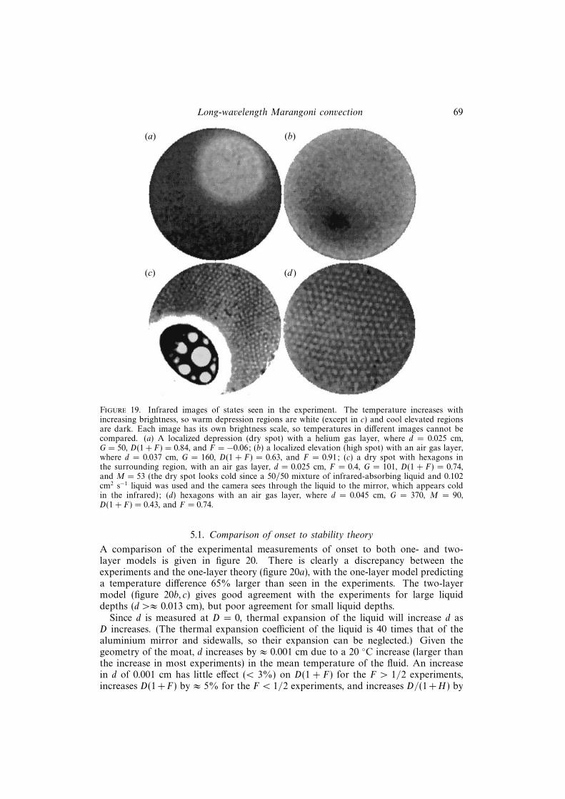
Figure 19. Infrared images of states seen in the experiment. The temperature increases withincreasing brightness, so warm depression regions are white (except in c) and cool elevated regionsare dark. Each image has its own brightness scale, so temperatures in different images cannot becompared. (a) A localized depression (dry spot) with a helium gas layer, where d = 0.025 cm,G = 50, D(1 + F) = 0.84, and F = −0.06; (b) a localized elevation (high spot) with an air gas layer,where d = 0.037 cm, G = 160, D(1 + F) = 0.63, and F = 0.91; (c) a dry spot with hexagons inthe surrounding region, with an air gas layer, d = 0.025 cm, F = 0.4, G = 101, D(1 + F) = 0.74,and M = 53 (the dry spot looks cold since a 50/50 mixture of infrared-absorbing liquid and 0.102cm2 s−1 liquid was used and the camera sees through the liquid to the mirror, which appears coldin the infrared); (d) hexagons with an air gas layer, where d = 0.045 cm, G = 370, M = 90,D(1 + F) = 0.43, and F = 0.74.

5.1. Comparison of onset to stability theory

A comparison of the experimental measurements of onset to both one- and two-layer models is given in figure 20. There is clearly a discrepancy between theexperiments and the one-layer theory (figure 20a), with the one-layer model predictinga temperature difference 65% larger than seen in the experiments. The two-layermodel (figure 20b, c) gives good agreement with the experiments for large liquiddepths (d >≈ 0.013 cm), but poor agreement for small liquid depths.

Since d is measured at D = 0, thermal expansion of the liquid will increase d asD increases. (The thermal expansion coefficient of the liquid is 40 times that of thealuminium mirror and sidewalls, so their expansion can be neglected.) Given thegeometry of the moat, d increases by ≈ 0.001 cm due to a 20 C increase (larger thanthe increase in most experiments) in the mean temperature of the fluid. An increasein d of 0.001 cm has little effect (< 3%) on D(1 + F) for the F > 1/2 experiments,increases D(1 +F) by ≈ 5% for the F < 1/2 experiments, and increases D/(1 +H) by


0.8

0.4

0

D1+H

0.005 0.010 0.015 0.020 0.025 0.030

d (cm)

(a)

0.8

0.4

0

D (1+F )

0.005 0.010 0.015 0.020 0.025 0.030

d (cm)

(b)

0.8

0.4

0

D (1+F )

0.2

F

(c)

0.4 0.6 0.8 0.6

Figure 20. Comparison of instability onset observed with increasing ∆T (increasing D) with thepredictions of (a) one-layer and (b, c) two-layer models. The theoretical prediction (taking intoaccount the correction factor (1 + 1/B) for finite cell size) in each case is given by the dashedline at 0.70. (a) The onset prediction of the one-layer model is 65% larger than observed in theexperiment. (b) The prediction of the two-layer model gives good agreement with the experimentsfor thick liquid depths, but there is a significant departure for thin depths. In (a) and (b), circlesare experiments in 0.102 cm2 s−1 viscosity silicone oil; squares are experiments performed in higherviscosity (≈ 0.30 cm2 s−1) silicone oil. No significant difference is seen between the different viscosityfluids, in agreement with theory. (c) In agreement with the two-layer nonlinear theory, there is aqualitative change in the instability around F = 1/2, where only localized depressions (circles) formfor F < 0.48 (left-hand arrow), only localized elevations (triangles) form for F > 0.58 (right-handarrow), and both states form for 0.48 < F < 0.58.


t=0:00 min 10:30 min 13:50 min

t=15:30 min 17:10 min 20:15 min

Figure 21. The evolution of a localized depression and formation of a dry spot in in-frared-absorbing silicone oil of depth d = 0.0267 ± 0.0008 cm, F = −0.07, D(1 + F) = 0.81 ± 0.04,D/(1 +H) = 0.41± 0.03, and helium in the gas layer. At t = 0 (an arbitrary starting point), there isnegligible deformation of the interface. The liquid layer begins to form a localized depression (thewhite circle) and in 15 minutes the interface has ruptured (hmin → 0) and formed a dry spot. The dryspot continues to grow for several more minutes before saturating. Bright regions are hot becausethey are closer to the heater; dark regions are cool because they are farther from the heater; allimages have the same intensity scaling.

≈ 6% ± 3% in the one-layer theory. In addition, the values of F would be increasedby less than 0.03 for F < 1/2 and by 0.03–0.07 for F > 1/2.

We do not include the onset values from the helium experiments in our datasince the helium experiments are not sufficiently controlled to permit quantitativecomparison with theory. Too fast a helium flow rate cools the interface and leads toartificially low values of D for onset; too slow a helium flow rate allows contaminationby air and leads to artificially high values of D for onset. For example, a 40% molefraction of air (60% helium) would lower the onset value of D in figures 19 and 21to the value predicted by the two-layer model. (It would also increase F from −0.06to 0.27, which is still less than 1/2.)

The steady-state deformation that we observe before the formation of the dry spotindicates the presence of a small amount of non-uniformity in the system. Even withψ1 = 0.005 (see §3.6), the interface deforms significantly (hmin ≈ 0.6–0.8, dependingon F) below the instability onset. Some of the variation in the onset values in thetwo-layer model may be due to the differing influence of non-uniformity on εc fordifferent F (see figures 15 and 20c), but the variation in εc due to differing F ismuch smaller in figure 15 than in figure 20c, which implies that a constant amountof non-uniformity cannot explain the varying discrepancy between experiment andtheory. We believe the sidewalls to be the largest source of non-uniformity in thesystem, but (3.33) cannot capture the influence of the sidewalls since we use periodic


(a) (b) (c)

Figure 22. A sequence of infrared images showing the evolution of a dry spot well above onset,including the formation of a high spot. (a) Higher-order structures can form when ∆T is increasedabove ε2 > 0 before the dry spot has a chance to develop. (b) As ∆T is increased further, the dryspot slowly increases in size. (c) When F and D in the region surrounding the dry spot becomesufficiently large, the liquid can become unstable to a high spot (upper-left corner) that pops up tothe sapphire window.

boundary conditions (i.e. no sidewalls). However, §3.6 and (3.33) at least give us asense of the effect of non-uniformity in the system.

5.2. Localized depressions (dry spots)

In most experiments, F < 1/2 and the liquid becomes unstable to a long-wavelengthinstability that leads to the formation of a dry spot of horizontal extent ∼ 100 × d(see figures 19a, 20c and 21). The area of the dry spot is typically 1/4–1/3 the area ofthe entire cell. Once the dry spot forms, fluid flow consists of steady-state convectionconcentrated at the edge of the dry spot. The dry spot is not completely dry since avery thin adsorbed layer remains (Burelbach et al. 1990).

The dry spot appears at different locations in different experiments, although itusually appears at the same location for multiple runs in a given experiment. When itappears near the centre of the cell, the dry spot closely approximates a circle; when itappears near the edge of the cell, it is oval-shaped with the short axis perpendicularto the sidewall. Before the formation of the dry spot, the interface exhibits steady-state deformation in a manner very similar to the non-uniformity-driven deformationshown in figure 14. Although the interface is initially flat in the central region,the sidewall causes non-uniformity at the edge of the cell even at ∆T = 0; thisnon-uniformity grows as D (i.e. ∆T ) is increased until the steady-state deformationbecomes unstable, which leads to the formation of the dry spot.

Higher-order structure (such as a large droplet trapped in the centre of the dryspot) can occur when D is increased above the critical value so that higher-ordermodes are unstable while the dry spot forms (see figure 22a). Once the dry spot hasformed fully, we observe no time-dependence with fixed control parameter, except anoccasional slow, transient migration of the dry spot after which the dry spot remainsstationary. As D is increased further, the dry spot slowly grows in size (see figure 22b).

5.3. Localized elevations (high spots)

The liquid layers in the experiment do not form dry spots for F >≈ 1/2 (see figure20c); rather, the liquid pops up to the top plate (sapphire window). This poppingup is predicted by the two-layer model, but not by the one-layer model, and thepop-up occurs consistently at the value of D predicted. In addition, the transitionfrom dry spot to high spot occurs near the predicted value of F = 1/2. As seen in


the simulations (see figures 8 and 9), the size of the high spot appears to be smallerthan that of the dry spot.

The liquid popping up to the top plate could be explained within the one-layermodel in that when a dry spot forms, the interface surrounding the forming dryspot must increase in elevation; for example, the rim of the forming dry spot, not alocalized elevation in the sense of the two-layer model, could be popping up to thetop plate. This argument is plausible since F > 1/2 experiments have thin air layers(dg ≈ 0.025 cm). We addressed this question by running pairs of experiments with thesame d and dg , but with different values of F . An experiment with F > 1/2 in air hasF ≈ 0 in helium gas. Thus, if a dry spot forms with helium, but the liquid pops upto the sapphire window with air, that could be an indication that we are observingthe predicted qualitative change of behaviour at F = 1/2. We obtained dry spots inhelium for experiments which in air would correspond to F = 0.75. This suggeststhat the elevated regions are not the rims of dry spots popping up due to the narrowgas layer. However, it is also possible that helium’s larger thermal conductivity (andthus smaller total temperature difference across the gas layer) reduces the amountof non-uniformity in the system. Alternatively, the larger heat fluxes required byhelium’s larger thermal conductivity may yield larger relative non-uniformities thanare present with air as the gas.

Infrared imaging, however, allows us to watch a localized elevation as it acceleratesupwards to the sapphire window (see figure 23) and to determine that we are observingpop-up due to a localized elevation, not the elevated rim of a forming dry spot. Whenthe high spot begins to form, there is no evidence of a localized depression. Theheight of a small region of the interface begins to increase and then rapidly acceleratesupwards until the liquid pops up to the top plate. In experiments with a very thinhelium layer, the high spot cannot form (F ≈ 0 in helium), but the rim of the dryspot pops up to the top plate because of the narrow gas layer. This situation iseasily distinguished from the localized elevation since the entire rim (not just a smallregion) approaches the sapphire window; as a localized elevation forms, the rest ofthe interface remains far from the sapphire window.

A localized elevation can appear in the system after the formation of the dry spotwhen F is near but less than 1/2. The initial dry spot drains approximately 1/3 ofthe cell and thus increases the mean thickness of the remainder of the cell by 50%.This increase in h can increase the local value of F above 1/2 and, if ∆T is increasedenough (above the onset of the dry spot), then the surrounding region can becomeunstable to a localized elevation (see figure 22c). Although the dry spot perturbs itssurrounding region, mostly by increasing the local liquid depth, its velocity field doesnot extend significantly past its perimeter (see figure 12a).

5.4. Competition with hexagons

We observe three different states at the onset of instability for F < 1/2. Forlarge G (independent of F), Benard hexagons form (figure 19d). For small G, thelong-wavelength dry spot forms (figures 19a, 24). For intermediate G, both thelong-wavelength (dry spot) and hexagonal modes appear together (figure 19c, 24).In this case, the long-wavelength deformational mode is linearly unstable and itsformation induces the formation of the hexagonal mode by increasing the local depthin the region surrounding the dry spot. When ∆T is increased above onset forthe long-wavelength mode, the dry spot continues to increase in size until eitherthe liquid pops up to the top plate (figure 22c) or the local value of M in thesurrounding elevated region is sufficiently large to cause the formation of hexagons


t=0:00 min 5:00 min 5:40 min

t=5:50 min 5:59 min 6:00 min

Figure 23. The evolution of a localized elevation and formation of a high spot that pops up to thetop plate. The experiment is performed in exactly the same conditions as figure 21 except that hereair was used as the gas (F = 0.65 ± 0.04, D(1 + F) = 0.73 ± 0.03). At t = 0 (an arbitrary startingpoint), there is negligible deformation of the interface. Five minutes later, a localized elevation (thedark oval) has begun to form, which in the span of a minute rapidly rises in elevation. At 5:59,the high spot is nearly touching the sapphire window and 1 s later the high spot has reached thesapphire window. Within 15 s (not shown), the liquid has wet nearly the entire top plate. Brightregions are hot because they are closer to the heater; dark regions are cool because they are fartherfrom the heater; all images have the same intensity scaling.

(figure 19c); the hexagons then inhibit any further growth of the dry spot (Golovin,Nepomnyashchy, & Pismen 1994, 1997). When the hexagonal mode appears first (forlarge G), the long-wavelength mode does not appear as a secondary instability. Sincethe time scale of formation of the hexagons is the vertical diffusion time (d2/κ ≈ 0.1s), while the time scale for the long-wavelength mode is the horizontal diffusion time(L2/κ ≈ 3 hours), quickly ramping the temperature above M = 80 allows formationof the hexagons as the primary instability even when the long-wavelength instabilitywould be primary if ∆T were increased quasi-statically, as assumed by linear theory.If ∆T is then decreased slowly below onset of hexagons, a dry spot can form oncethe hexagons have disappeared.

For small F and H , the transition depth dt from dry spots to hexagons is predictedto be

dt ≈(120νκ/g

)1/3. (5.1)

(There is an H- and F-dependence but it is weak because of the cubic root.) Inthe 0.102 cm2 s−1 silicone oil with air as the gas layer, we see the transition fromlong-wavelength to hexagons at dt = 0.024 ± 0.001 cm, close to the prediction ofdt = 0.023 ± 0.001 cm. Using either a large F or helium in the gas layer shifts thelong-wavelength/hexagon transition depth. The formation of the dry spot induces


0.8

0.4

0

D (1+F )

0.005 0.010 0.015 0.020 0.025

d (cm)

Figure 24. Experimental data for the onset of instability with increasing ∆T in 0.102 cm2 s−1

silicone oil with an air gas layer and F < 1/2. The two-layer model prediction is given by thedashed line at D(1 + F) = 0.70. The transition from dry spots (circles) to dry spots with hexagonsin the surrounding region (triangles) occurs around d = 0.017 cm (vertical arrow). Above d = 0.024cm, hexagons are the primary instability.

hexagons in the elevated region of the cell for d > 0.017 cm. This transition depthis F-dependent since the change in the local vertical temperature difference is F-dependent (see (3.3)); in our experiments, F = 0.3–0.5 near the transition from dryspots to dry-spot-induced hexagons.

The steady-state deformation before onset of the instability blurs the distinctionbetween dry-spot-induced hexagons and hexagons near dt. For d slightly less than dt,the hexagons form in part of the cell due to the steady-state deformation, but theliquid still becomes unstable to the dry spot. For d slightly above dt, the hexagons fillthe entire cell before the liquid can become unstable to the long-wavelength instability,but the interface is severely deformed.

6. ConclusionsTwo modes of instability exist in surface-tension-driven Benard–Marangoni con-

vection where the liquid is heated from below and cooled from above. The short-wavelength hexagonal mode (q = 1.99) occurs for large G, when diffusion is theimportant (slow) stabilizing mechanism. The long-wavelength deformational mode(q = 2πd/L 1) occurs for small G, when gravity is the important (slow) stabilizingmechanism. This long-wavelength instability can take the form of either a localizeddepression that evolves to a dry spot, or a localized elevation (high spot) that acceler-ates upwards and causes the liquid to pop up to the top plate. The relative thicknessesand thermal conductivities of the liquid and gas layers determine whether the dryspot or high spot forms: a high spot forms where the liquid thermal conductivity ismuch larger than the gas thermal conductivity and the liquid depth is nearly equalto or greater than the gas depth. The deformation due to the long-wavelength modecan cause the formation of the hexagonal mode by increasing the local value of Mabove the critical value for the hexagons.

The long-wavelength instability is described by an evolution equation for the heightof the interface. Analysis of the evolution equation predicts that the instability issubcritical and that the unstable, backwards branch of the bifurcation curve neverturns over to a stable branch. Numerical simulations of the evolution equation revealstates that agree qualitatively with states seen in the experiment.


Experimental study of the long-wavelength mode shows that a two-layer model isnecessary to describe the onset of the deformational long-wavelength mode. The onsetprediction of the two-layer model comes closer to the experimental measurements ofonset than does the prediction of the one-layer model, although at thin liquid depthsthere is significant deviation between two-layer theory and experiment. For these thinliquid depths, the onset occurs earlier in experiment than predicted. In addition, theexperiments exhibit steady-state deformation before onset of the instability. Both thepremature onset and steady-state deformation are indications of non-uniformities inthe experiment. Theoretical analysis of the influence of non-uniformity in heatingshows that even small (1%) non-uniformities in the imposed temperature differencecan cause large (∼ 30%) deformations of the interface before the interface becomesunstable to the long-wavelength instability. Small non-uniformities in heating alsocause the instability to occur at smaller temperature differences than predicted bytheory, though this shift in onset is not as large as seen in the experiment. Non-uniformities due to the sidewall are the most likely culprit and we have beguna theoretical study of the effect of the sidewalls upon the formation of the long-wavelength instability.

Marangoni convection experiments aboard Apollo 14 (Grodzka & Bannister 1972)and Apollo 17 (Grodzka & Bannister 1975) yielded Benard convection cells, andnot the long-wavelength instability, even though G < 1. Several factors explainwhy the long-wavelength instability was not observed in the Apollo experiments.Fast ramping was used in the experiments since onset occurred at around 30 s –of order the vertical diffusion time (d2/κ) – after initiation of the experiment; asmentioned in §5.4, fast ramping allows hexagons to form for smaller G than predictedby stability theory. More importantly, however, the long-wavelength onset conditionin microgravity can differ greatly from the onset condition in terrestrial gravity.According to (3.15), the correction to the q = 0 onset condition for an experiment offinite size with fundamental physical wavenumber q = 2π/L (rescaled wavenumberq = 1) is a factor of (1 + 1/B); since B ∝ g, in microgravity this correction factorbecomes large and increases the long-wavelength onset in a finite-size cell by ordersof magnitude. (In the Apollo experiments, the finite cell size correction shifted theonset of the long-wavelength mode to M ∼ 280, above the onset of hexagons). Ingeneral, both surface tension and gravity stabilize the long-wavelength deformationalinstability. The static Bond number B characterizes the relative importances of thesetwo stabilizing effects. When L dcap (B 1), where dcap = (σ/ρg)1/2 is the capillarylength, gravity plays the dominant stabilizing role and D = 2G/3(1 + F) (with asmall correction due to surface tension) is the onset condition. When L dcap(B 1), surface tension plays the dominant stabilizing role and DB = 2/3(1 + F),or MCr = σT∆T/σ = 2(2πd/L)2/3(1 + F) (with a small correction due to gravity), isthe onset condition. In our terrestrial experiments, L = 26.5dcap (B = 18) so surfacetension plays no significant role. In microgravity experiments, L dcap (L ∼ 0.06dcapin the Apollo experiments) so surface tension plays the dominant stabilizing rolefor the long-wavelength instability; that is, the destabilization by thermocapillaritycompetes with the stabilization by surface tension, not gravity.

The authors thank Kirk Brattkus, Stephen Davis, Robert Kelly, and Philip Morrisonfor useful discussions. This research is supported by the NASA Microgravity Scienceand Applications Division (Grant No. NAG3-1839), the Office of Naval Research(Grant No. N00014-89-J-1495), and a NASA ESS Cooperative Agreement (NCCS5-154). S.J.V.H. is supported by the NASA Graduate Student Researchers Program.


REFERENCES

Benard, H. 1900 Les tourbillons cellulaires dans une nappe liquide. Rev. Gen. Sci. Pure Appl. 11,1261–1271, 1309–1328.

Bertozzi, A. L., Brenner, M. P., Dupont, T. F. & Kadanoff, L. P. 1994 Singularities and similaritiesin interface flows. In Trends and Perspectives in Applied Mathematics (ed. L. Sirovich), pp. 155–208. Springer.

Block, M. J. 1956 Surface tension as the cause of Benard cells and surface deformation in a liquidfilm. Nature 178, 650.

Burelbach, J. P., Bankoff, S. G. & Davis, S. H. 1990 Steady thermocapillary flows of thin liquidlayers. II. Experiment. Phys. Fluids A 2, 322–333.

Canuto, C., Hussaini, M. Y., Quateroni, A. & Zang, T. A. 1987 Spectral Methods in Fluid Dynamics,p. 84. Springer.

Cloot, A. & Lebon, G. 1984 A nonlinear stability analysis of the Benard-Marangoni problem. J.Fluid Mech. 145, 447–469.

Cross, M. C. & Hohenberg, P. C. 1993 Pattern formation outside of equilibrium. Rev. Mod. Phys.65, 851–1112.

Davis, S. H. 1983 Rupture of thin liquid films. In Waves on Fluid Interfaces (ed. R. E. Meyer), pp.291–302. Academic.

Davis, S. H. 1987 Thermocapillary instabilities. Ann. Rev. Fluid Mech. 19, 403–435.

Davis, S. H. & Homsy, G. M. 1980 Energy stability theory for free-surface problems: buoyancy-thermocapillary layers. J. Fluid Mech. 98, 527–553.

Deissler, R. J. & Oron, A. 1992 Stable localized patterns in thin liquid films. Phys. Rev. Lett. 68,2948–2951.

Funada, T. 1987 Nonlinear surface waves driven by the Marangoni instability in a heat transfersystem. J. Phys. Soc. Japan 56, 2031–2038.

Garcia-Ybarra, P. L., Castillo, J. L. & Velarde, M. G. 1987 A nonlinear evolution equation forBenard-Marangoni convection with deformable boundary. Phys. Lett. A 122, 107–110.

Goldstein, R. E., Pesci, A. I. & Shelley, M. J. 1995 Attracting manifold for a viscous topologytransition. Phys. Rev. Lett. 75, 3665–3668.

Golovin, A. A., Nepomnyashchy, A. A. & Pismen, L. M. 1994 Interaction between short-scaleMarangoni convection and long-scale deformational instability. Phys. Fluids 6, 34–48.

Golovin, A. A., Nepomnyashchy, A. A. & Pismen, L. M. 1997 Nonlinear evolution and secondaryinstabilities of Marangoni convection in a liquid-gas system with deformable interface. J. FluidMech. 341, 317–341.

Goussis, D. A. & Kelly, R. E. 1990 On the thermocapillary instabilities in a liquid layer heatedfrom below. Intl J. Heat Mass Transfer 33, 2237–2245.

Grodzka, P. G. & Bannister, T. C. 1972 Heat flow and convection demonstration experimentsaboard Apollo 14. Science 176, 506–508.

Grodzka, P. G. & Bannister, T. C. 1975 Heat flow and convection experiments aboard Apollo 17.Science 187, 165–167.

Hadji, L., Safar, J. & Schell, M. 1991 Analytical results on the coupled Benard-Marangoniproblem consistent with experiment. J. Non-Equilib. Thermodyn. 16, 343–356.

Joo, S. W., Davis, S. H. & Bankoff, S. G. 1991 Long-wave instabilities of heated falling films. J.Fluid Mech. 230, 117–146.

Kopbosynov, B. K. & Pukhnachev, V. V. 1986 Thermocapillary flow in thin liquid films. FluidMech. Sov. Res. 15, 95–106.

Koschmieder, E. L. & Biggerstaff, M. I. 1986 Onset of surface-tension-driven Benard convection.J. Fluid Mech. 167, 49–64.

Krishnamoorthy, S. & Ramaswamy, B. 1995 Spontaneous rupture of thin liquid films due tothermocapillarity: A full-scale direct numerical simulation. Phys. Fluids 7, 2291–2293.

Nepomnyashchii, A. A. & Simanovskii, I. B. 1990 Long-wave thermocapillary convection in layerswith deformable interfaces. Appl. Math. Mech. 54, 490–496.

Nield, D. A. 1964 Surface tension and buoyancy effects in cellular convection. J. Fluid Mech. 19,341–352.

Oron, A. & Rosenau, P. 1992 Formation of patterns induced by thermocapillarity and gravity. J.Phys. II (Paris) 2, 131–146.


Pantaloni, J., Bailleux, R, Salan, J. & Velarde, M. G. 1979 Rayleigh-Benard-Marangoniinstability: New experimental results. J. Non-Equilib. Thermodyn. 4, 201–218.

Pearson, J. R. A. 1958 On convection cells induced by surface tension. J. Fluid Mech. 4, 489–500.

Perez-Garcia, C. & Carneiro, G. 1991 Linear stability analysis of Benard-Marangoni convectionin fluids with a deformable free surface. Phys. Fluids A 3, 292–298.

Rasenat, S., Hartung, G. Winkler, B. L. & Rehberg, I. 1989 The shadowgraph method inconvection experiments. Exps. Fluids 7, 412-420.

Scanlon, J. W. & Segel, L. A. 1967 Finite amplitude cellular convection induced by surface tension.J. Fluid Mech. 30, 149–162.

Schatz, M. F. & Howden, K. 1995 Purification of silicone oils for fluid experiments. Exps. Fluids19, 359–361.

Schatz, M. F., VanHook, S. J., McCormick, W. D., Swift, J. B. & Swinney, H. L. 1995 Onset ofsurface-tension-driven Benard convection. Phys. Rev. Lett. 75, 1938–1941.

Scriven, L. E. & Sternling, C. V. 1964 On cellular convection driven by surface-tension gradients:effects of mean surface tension and surface viscosity. J. Fluid Mech. 19, 321–340.

Sivashinsky, G. I. 1982 Large cells in nonlinear Marangoni convection. Physica D 4, 227–235.

Smith, K. A. 1966 On convective instability induced by surface-tension gradients. J. Fluid Mech. 24,401–414.

Takashima, M. 1970 Surface-tension-driven convection with boundary slab of finite conductivity.J. Phys. Soc. Japan 29, 531.

Takashima, M. 1981a Surface tension driven instability in a horizontal liquid layer with a deformablefree surface. I. Stationary convection. J. Phys. Soc. Japan 50, 2745–2750.

Takashima, M. 1981b Surface tension driven instability in a horizontal liquid layer with a deformablefree surface. II. Overstability. J. Phys. Soc. Japan 50, 2751–2756.

Tan, M. J., Bankoff, S. G. & Davis, S. H. 1990 Steady thermocapillary flows of thin liquid layers.I. Theory. Phys. Fluids A 2, 313–321.

VanHook, S. J, Schatz, M. F., McCormick, W. D., Swift, J. B. & Swinney, H. L. 1995 Long-wavelength instability in surface-tension-driven Benard convection. Phys. Rev. Lett. 75, 4397–4400.

Wilson, S. K. 1993 The effect of a uniform magnetic field on the onset of steady Benard-Marangoniconvection in a layer of conducting fluid. J. Engng Maths 27, 161–188.

Long-wavelength surface-tension-driven Benard …chaos.ph.utexas.edu/manuscripts/1081888161.pdf ·...

Documents

Transcript of Long-wavelength surface-tension-driven Benard …chaos.ph.utexas.edu/manuscripts/1081888161.pdf ·...