Frontiers of Cosmic Ray Science 205

Long-Term Variations of Cosmic Rays and TerrestrialEnvironment

Ilya G. Usoskin

Sodankyla Geophys. Observatory (Oulu unit), University of Oulu, Finland

Ilya.Usoskin@oulu.fi

Abstract

This rapporteur talk aims to review scientific contributions to the following ses-

sions of the 28th International Cosmic Ray Conference (August 2003, Tsukuba,

Japan): SH 3.4 “Long-term variations,” SH 3.5 “Long-term variation of cosmic

rays studied by cosmogenic nuclides,” SH 3.6 “Terrestrial effects and cosmogenic

nuclides” and partly SH 1.5 “Instrumentation and new projects.” Most important

results are discussed in the line of long-term cosmic ray variations and terrestrial

effects.

1. Introduction

Many interesting contributions have been presented at the 28th ICRC

about long-term variations of cosmic rays and terrestrial environment (sessions

SH 3.4–SH 3.6 and partly SH 1.5), and it is impossible to cover all of them

in this brief review. The selection is subjective, and the primary attention is

given to new experimental results and their interpretation. Some statistics of the

presented papers and their topical subdivision is summarized Table 1. Although

the dispersion of individual paper’s topics is quite broad, they generally fit into two

main directions, long-term cosmic ray variations and the terrestrial environment.

References to the 28th ICRC contribution papers are given using the Session and

page numbers in the ICRC Proceeding volumes.

2. Cosmogenic proxies of cosmic rays

In nuclear collisions of energetic cosmic rays with targets in the Earth’s

atmosphere, numerous secondaries are produced. Some of them are radioactive

isotopes and have no other natural sources but cosmic rays. After production and

complicated transport in the atmosphere, such cosmogenic isotopes can be stored

in various natural archives. Their content in the archive is measured nowadays to

estimate the cosmic ray flux in the past. The main advantage of this method is its

pp. 205–228 c©2004 by Universal Academy Press, Inc.

206

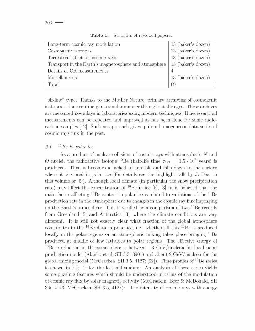
Table 1. Statistics of reviewed papers.

Long-term cosmic ray modulation 13 (baker’s dozen)

Cosmogenic isotopes 13 (baker’s dozen)

Terrestrial effects of cosmic rays 13 (baker’s dozen)

Transport in the Earth’s magnetosphere and atmosphere 13 (baker’s dozen)

Details of CR measurements 4

Miscellaneous 13 (baker’s dozen)

Total 69

“off-line” type. Thanks to the Mother Nature, primary archiving of cosmogenic

isotopes is done routinely in a similar manner throughout the ages. These archives

are measured nowadays in laboratories using modern techniques. If necessary, all

measurements can be repeated and improved as has been done for some radio-

carbon samples [12]. Such an approach gives quite a homogeneous data series of

cosmic rays flux in the past.

2.1. 10Be in polar ice

As a product of nuclear collisions of cosmic rays with atmospheric N and

O nuclei, the radioactive isotope 10Be (half-life time τ1/2 = 1.5 · 106 years) is

produced. Then it becomes attached to aerosols and falls down to the surface

where it is stored in polar ice (for details see the highlight talk by J. Beer in

this volume or [5]). Although local climate (in particular the snow precipitation

rate) may affect the concentration of 10Be in ice [5], [3], it is believed that the

main factor affecting 10Be content in polar ice is related to variations of the 10Be

production rate in the atmosphere due to changes in the cosmic ray flux impinging

on the Earth’s atmosphere. This is verified by a comparison of two 10Be records

from Greenland [5] and Antarctica [3], where the climate conditions are very

different. It is still not exactly clear what fraction of the global atmosphere

contributes to the 10Be data in polar ice, i.e., whether all this 10Be is produced

locally in the polar regions or an atmospheric mixing takes place bringing 10Be

produced at middle or low latitudes to polar regions. The effective energy of10Be production in the atmosphere is between 1.3 GeV/nucleon for local polar

production model (Alanko et al. SH 3.3, 3901) and about 2 GeV/nucleon for the

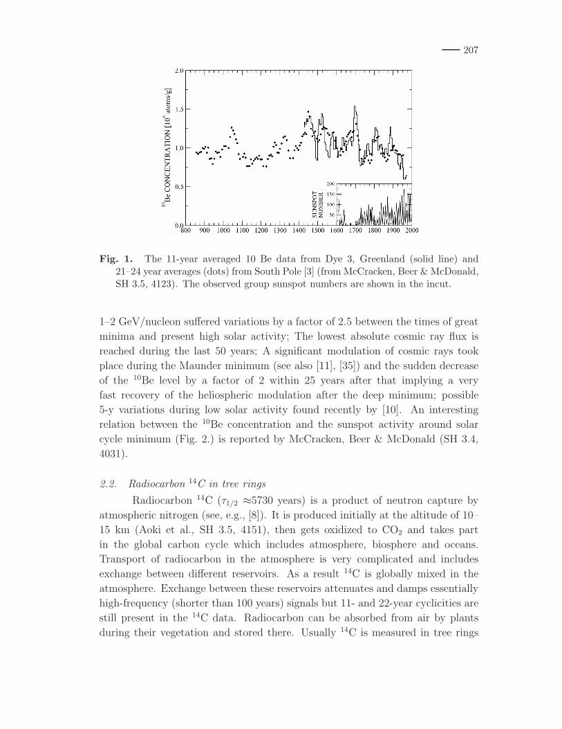
global mixing model (McCracken, SH 3.5, 4127; [22]). Time profiles of 10Be series

is shown in Fig. 1. for the last millennium. An analysis of these series yields

some puzzling features which should be understood in terms of the modulation

of cosmic ray flux by solar magnetic activity (McCracken, Beer & McDonald, SH

3.5, 4123; McCracken, SH 3.5, 4127): The intensity of cosmic rays with energy

207

Fig. 1. The 11-year averaged 10 Be data from Dye 3, Greenland (solid line) and21–24 year averages (dots) from South Pole [3] (from McCracken, Beer & McDonald,SH 3.5, 4123). The observed group sunspot numbers are shown in the incut.

1–2 GeV/nucleon suffered variations by a factor of 2.5 between the times of great

minima and present high solar activity; The lowest absolute cosmic ray flux is

reached during the last 50 years; A significant modulation of cosmic rays took

place during the Maunder minimum (see also [11], [35]) and the sudden decrease

of the 10Be level by a factor of 2 within 25 years after that implying a very

fast recovery of the heliospheric modulation after the deep minimum; possible

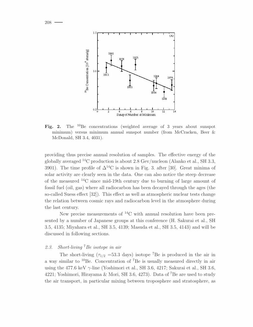
5-y variations during low solar activity found recently by [10]. An interesting

relation between the 10Be concentration and the sunspot activity around solar

cycle minimum (Fig. 2.) is reported by McCracken, Beer & McDonald (SH 3.4,

4031).

2.2. Radiocarbon 14C in tree rings

Radiocarbon 14C (τ1/2 ≈5730 years) is a product of neutron capture by

atmospheric nitrogen (see, e.g., [8]). It is produced initially at the altitude of 10–

15 km (Aoki et al., SH 3.5, 4151), then gets oxidized to CO2 and takes part

in the global carbon cycle which includes atmosphere, biosphere and oceans.

Transport of radiocarbon in the atmosphere is very complicated and includes

exchange between different reservoirs. As a result 14C is globally mixed in the

atmosphere. Exchange between these reservoirs attenuates and damps essentially

high-frequency (shorter than 100 years) signals but 11- and 22-year cyclicities are

still present in the 14C data. Radiocarbon can be absorbed from air by plants

during their vegetation and stored there. Usually 14C is measured in tree rings

208

Fig. 2. The 10Be concentrations (weighted average of 3 years about sunspotminimum) versus minimum annual sunspot number (from McCracken, Beer &McDonald, SH 3.4, 4031).

providing thus precise annual resolution of samples. The effective energy of the

globally averaged 14C production is about 2.8 Gev/nucleon (Alanko et al., SH 3.3,

3901). The time profile of ∆14C is shown in Fig. 3. after [30]. Great minima of

solar activity are clearly seen in the data. One can also notice the steep decrease

of the measured 14C since mid-19th century due to burning of large amount of

fossil fuel (oil, gas) where all radiocarbon has been decayed through the ages (the

so-called Suess effect [32]). This effect as well as atmospheric nuclear tests change

the relation between cosmic rays and radiocarbon level in the atmosphere during

the last century.

New precise measurements of 14C with annual resolution have been pre-

sented by a number of Japanese groups at this conference (H. Sakurai et al., SH

3.5, 4135; Miyahara et al., SH 3.5, 4139; Masuda et al., SH 3.5, 4143) and will be

discussed in following sections.

2.3. Short-living 7Be isotope in air

The short-living (τ1/2 =53.3 days) isotope 7Be is produced in the air in

a way similar to 10Be. Concentration of 7Be is usually measured directly in air

using the 477.6 keV γ-line (Yoshimori et al., SH 3.6, 4217; Sakurai et al., SH 3.6,

4221; Yoshimori, Hirayama & Mori, SH 3.6, 4273). Data of 7Be are used to study

the air transport, in particular mixing between troposphere and stratosphere, as

209

-30

-20

-10

0

10

20

1000 1200 1400 1600 1800 2000

14

C (

per

mill

e)

MMSM

WM

OM

Fig. 3. Time profile of decadal 14C data [30]. Most recent great minima of solaractivity are marked: Oort minimum (OM), Wolf minimum (WM), Sporer minimum(SM) and Maunder minimum (MM).

well as the effect of solar energetic particle (SEP) events.

Yoshimori et al. (SH 3.6, 4217) studied seasonal variations of 7Be concen-

tration and found a strong increase during the Spring and a less reliable peak

in the Fall (Fig. 4.). Since the bulk of 7Be is produced in stratosphere while the

measurements are performed in the troposphere, mixing of air masses between the

two regions should result in enhanced concentration of 7Be at the surface level.

Accordingly, the found seasonal variations are interpreted by Yoshimori et al. as

evidence for tropospheric/stratospheric air mass mixing (e.g., [9],[2]) which takes

place in Spring and, probably, also in the Fall.

Sakurai et al. (SH 3.6, 4221) studied the quasi-periodic variations of 7Be

data with the synodic solar rotation period (26–27 days). The superposed epoch

analysis of 26-day folded data of 7Be, sunspot numbers and cosmic ray flux (mea-

sured by neutron monitors) is shown in Fig. 5. The 26-day periodicity is clearly

seen in 7Be concentration in phase (with few days delay) with cosmic ray data, in

agreement with the cosmogenic nature of these data. However, one can also see a

strong 13-day periodicity in phase with sunspot activity which is only marginally

present in cosmic ray data. This 13-day periodicity may indicate a solar influence

on 7Be production.

2.4. 44Ti in meteorites

Results of 44Ti measurements in meteorites have been presented by Cini

Castagnoli et al. (SH 3.4, 4045). During their life, meteorites are subject of con-

tinuous bombarding by cosmic rays which can produce radioactive isotopes in

their bodies. One such isotope is 44Ti (τ1/2 ≈59 years) which is a product of

nuclear interaction of cosmic protons with Fe and Ni. The abundance of 44Ti in

210

Fig. 4. Seasonal variations of 7Be concentrations since 01.01.2002 (from Yoshimori etal., SH 3.6, 4217). Black and gray lines indicate Spring and Fall peaks, respectively.

Fig. 5. 7Be concentrations, sunspot numbers, and neutron monitor data (multipliedby a factor of 30) folded with the folding period of 26 days for the each time series(from Sakurai et al., SH 3.6, 4221).

211

4

5

6

7

8

1700 1750 1800 1850 1900 1950

44T

i in

met

eori

tes

Fig. 6. Measurements of 44Ti in different chondrites together with the long-termtrend (after Cini Castagnoli et al., SH 3.4, 4045).

fallen stony meteorites can be measured and gives the intensity of cosmic rays in-

tegrated over the meteorite’s path. Accordingly, such an approach provides a kind

of cosmic ray space probing, i.e., beyond the geomagnetic and atmospheric effects.

However, since only the integrated flux can be measured, the time resolution of

this method is limited by the isotope’s life time.

2.5. Nitrates in polar ice

Another promising proxy is the concentration of nitrates and nitrites (called

NO(Y)) in polar ice. Production of NO(Y) in polar atmosphere is greatly en-

hanced during strong solar energetic particle (SEP) events with the total fluence

of protons (>30 MeV) exceeding 109 cm−2 [38], [13], [23]. After precipitation,

NO(Y) can be stored in polar ice where its content can be measured. Accord-

ingly, data on NO(Y) in polar ice is an index of strong SEP events in the past.

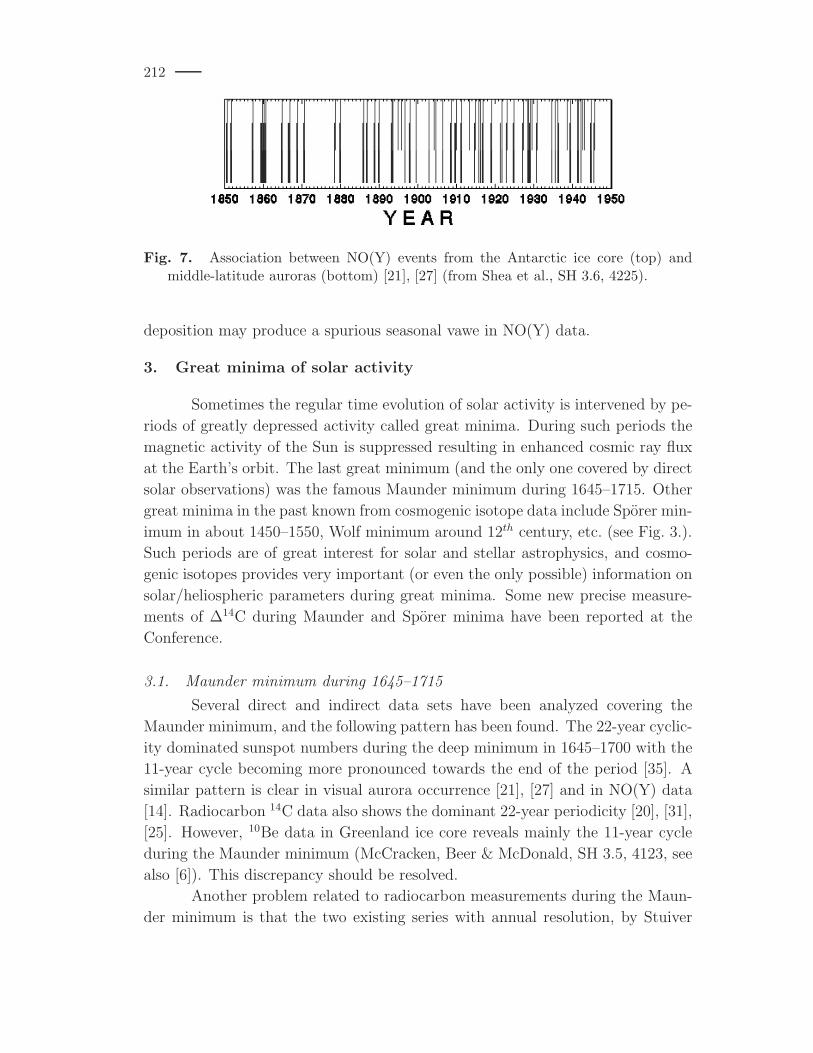
Shea et al. (SH 3.6, 4225) studied the relations between NO(Y) data from Antarc-

tic ice core and auroras visible in middle latitudes that serves as an index of very

strong interplanetary transient phenomenae (Fig. 7.). About 86% (51 out of 59)

of the analyzed mid-latitude aurora sightings have clear association with NO(Y)

events. This provides further evidence for the solar origin of NO(Y) peaks in

polar ice. Moreover, so high correlation of transient and energetic particle phe-

nomenae may indicate that SEP events with largest total fluence are related to

CME-driven shocks rather than to solar flares.

Shea et al. (SH 3.6, 4225) reported also a statistically significant season

dependence of nitrate peaks. No apparent reason is suggested for such a de-

pendence providing the correct timing of data. Although annual layers can be

identified in ice with high accuracy, distribution of samples within the annual ice

layer was supposed to be linear. Accordingly, seasonal variations in the local snow

212

Fig. 7. Association between NO(Y) events from the Antarctic ice core (top) andmiddle-latitude auroras (bottom) [21], [27] (from Shea et al., SH 3.6, 4225).

deposition may produce a spurious seasonal vawe in NO(Y) data.

3. Great minima of solar activity

Sometimes the regular time evolution of solar activity is intervened by pe-

riods of greatly depressed activity called great minima. During such periods the

magnetic activity of the Sun is suppressed resulting in enhanced cosmic ray flux

at the Earth’s orbit. The last great minimum (and the only one covered by direct

solar observations) was the famous Maunder minimum during 1645–1715. Other

great minima in the past known from cosmogenic isotope data include Sporer min-

imum in about 1450–1550, Wolf minimum around 12th century, etc. (see Fig. 3.).

Such periods are of great interest for solar and stellar astrophysics, and cosmo-

genic isotopes provides very important (or even the only possible) information on

solar/heliospheric parameters during great minima. Some new precise measure-

ments of ∆14C during Maunder and Sporer minima have been reported at the

Conference.

3.1. Maunder minimum during 1645–1715

Several direct and indirect data sets have been analyzed covering the

Maunder minimum, and the following pattern has been found. The 22-year cyclic-

ity dominated sunspot numbers during the deep minimum in 1645–1700 with the

11-year cycle becoming more pronounced towards the end of the period [35]. A

similar pattern is clear in visual aurora occurrence [21], [27] and in NO(Y) data

[14]. Radiocarbon 14C data also shows the dominant 22-year periodicity [20], [31],

[25]. However, 10Be data in Greenland ice core reveals mainly the 11-year cycle

during the Maunder minimum (McCracken, Beer & McDonald, SH 3.5, 4123, see

also [6]). This discrepancy should be resolved.

Another problem related to radiocarbon measurements during the Maun-

der minimum is that the two existing series with annual resolution, by Stuiver

213

Fig. 8. Time profile of 14C measurements around the Maunder minimum: by Stuiver[30] (thick curve), by Kocharov et al. [20] (thin curves) and by Masuda et al. (SH3.5, 4143) (dots).

et al. [30] (US East cost) and by Kocharov et al. [20] (Ural region and Western

Ukraine), depict different levels of ∆14C variations during the Maunder minimum

(Fig. 8.). Although an inter-calibration of the two series has been performed [12],

a possible source of the different level of ∆14C variations was still unclear. New

independent measurement of ∆14C in a Japanese cedar tree with annual resolu-

tion have been presented by Masuda et al. (SH 3.5, 4143) for the late phase of

the Maunder minimum (Fig. 8.). While being different from the two other series,

the new Japanese series depicts large variations of ∆14C during the second half

of the Maunder minimum, similar to Kocharov et al. series. Unfortunately, data

for the earlier part of the minimum are not available yet, and we look forward for

the whole Maunder minimum covered by the new measurements. This will also

clarify the relation between solar cycles during that period.

3.2. Sporer minimum in XV century

The Sporer minimum took place around 1400–1550. It is not well covered

by high resolution data, only 10Be data from Greenland were available for this

period with nearly annual resolution [5]. At this Conference, the results of new

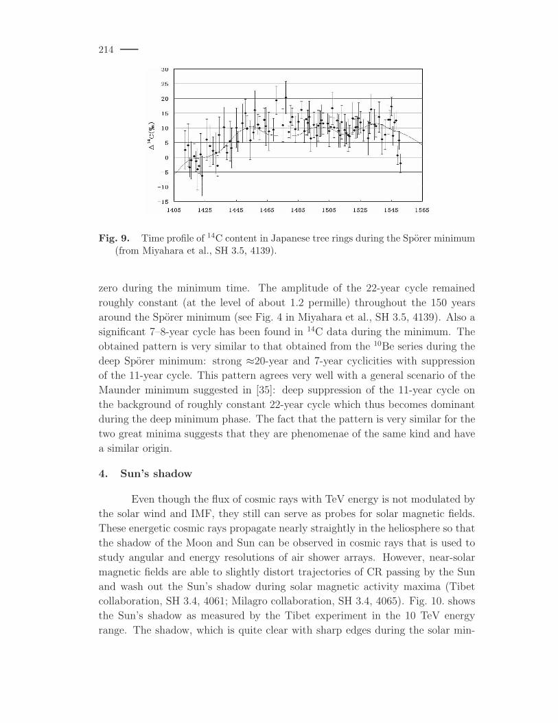
measurements of ∆14C in Japanese cedar tree performed by Miyahara et al. (SH

3.5, 4139) with annual resolution, covering the whole Sporer minimum, have been

presented. A preliminary spectral analysis of the radiocarbon data reveals the fol-

lowing main periodicities during the Sporer minimum. The amplitude of 11-year

cycle was greatly reduced from about 4 permille outside the minimum to nearly

214

Fig. 9. Time profile of 14C content in Japanese tree rings during the Sporer minimum(from Miyahara et al., SH 3.5, 4139).

zero during the minimum time. The amplitude of the 22-year cycle remained

roughly constant (at the level of about 1.2 permille) throughout the 150 years

around the Sporer minimum (see Fig. 4 in Miyahara et al., SH 3.5, 4139). Also a

significant 7–8-year cycle has been found in 14C data during the minimum. The

obtained pattern is very similar to that obtained from the 10Be series during the

deep Sporer minimum: strong ≈20-year and 7-year cyclicities with suppression

of the 11-year cycle. This pattern agrees very well with a general scenario of the

Maunder minimum suggested in [35]: deep suppression of the 11-year cycle on

the background of roughly constant 22-year cycle which thus becomes dominant

during the deep minimum phase. The fact that the pattern is very similar for the

two great minima suggests that they are phenomenae of the same kind and have

a similar origin.

4. Sun’s shadow

Even though the flux of cosmic rays with TeV energy is not modulated by

the solar wind and IMF, they still can serve as probes for solar magnetic fields.

These energetic cosmic rays propagate nearly straightly in the heliosphere so that

the shadow of the Moon and Sun can be observed in cosmic rays that is used to

study angular and energy resolutions of air shower arrays. However, near-solar

magnetic fields are able to slightly distort trajectories of CR passing by the Sun

and wash out the Sun’s shadow during solar magnetic activity maxima (Tibet

collaboration, SH 3.4, 4061; Milagro collaboration, SH 3.4, 4065). Fig. 10. shows

the Sun’s shadow as measured by the Tibet experiment in the 10 TeV energy

range. The shadow, which is quite clear with sharp edges during the solar min-

215

Fig. 10. Yearly variations of the Suns shadow at 10 TeV energy observed by Tibet-IIin 1996–1999 (from Amenomori et al. (Tibet collaboration), SH 3.4, 4061).

imum (1996), is washed out around the solar maximum. Accordingly, the Sun’s

shadow in CR is strongly affected by IMF depicting the solar cycle dependence. A

possible south-eastwards displacement of the shadow around maximum was also

reported by the Tibet group but not not confirmed by the Milagro group.

5. Environmental monitoring

Several contributions presenting different aspects of environmental moni-

toring have been presented. The measurements of 7Be in the air have been dis-

cussed above. Atmospheric neutrons produced by nuclear interactions of cosmic

rays with the atmospheric matter form the most important factor for radiation

doses. Zanini et al. (SH 3.6, 4291) presented measurements of fluxes and spectra

of atmospheric neutrons at different locations, altitude and weather conditions.

Cattani et al. (SH 3.6, 4181) have shown that washing out of natural and cosmic

ray induced radioactivity during rainout episodes results in enhanced radioactiv-

ity level as measured on the ground. Cattani et al. (SH 3.6, 4295) reported also

measurements of γ-ray spectra at different atmospheric depths and locations. En-

vironmental radioactivity measurements by SONTEL (Solar neutron telescope)

at Gornergrat, Switzerland have been performed by Butikofer et al. (SH 3.6, 4189)

to show that count rates due to natural radon presence may mimic possible solar

neutron signal.

6. Long-term cosmic ray intensity

Although cosmogenic isotopes serve as a proxy of cosmic ray intensity, it is

not straightforward to reconstruct the flux of cosmic rays in the past from these

data because of the complicated atmospheric transport of the isotopes before de-

position. A model has been presented to calculate the expected cosmic ray flux for

the last 400 years starting from solar activity (Usoskin et al., SH 3.4, 4041; Cini

216

Castagnoli et al., SH 3.4, 4045) using the following approach. Recently, Solanki

et al. [28] developed a semi-empirical model to calculate the open solar magnetic

flux from sunspot data (see Fig. 11.b). Bearing in mind that the open magnetic

flux is directly related to the globally averaged IMF which, in turn, defines the

long-term heliospheric modulation of cosmic rays, it can be converted to the so-

called modulation potential Φ [15] (Fig. 11.c). This modulation potential has

the meaning of the average rigidity loss of CR particles during their heliospheric

transport and defines the differential spectrum of CR in the Earth’s vicinity. Ac-

cordingly, CR flux is calculated since 1610 in terms of the standard polar neutron

monitor count rate (Fig. 11.d) which agrees pretty well with the actual NM count

rate for the last 50 years. Fig. 11.e presents a direct comparison of the calcu-

lated 10Be production in polar atmosphere with the actual 10Be measurements in

Greenland [5] and in Antarctica [3]. A good agreement between the reconstructed

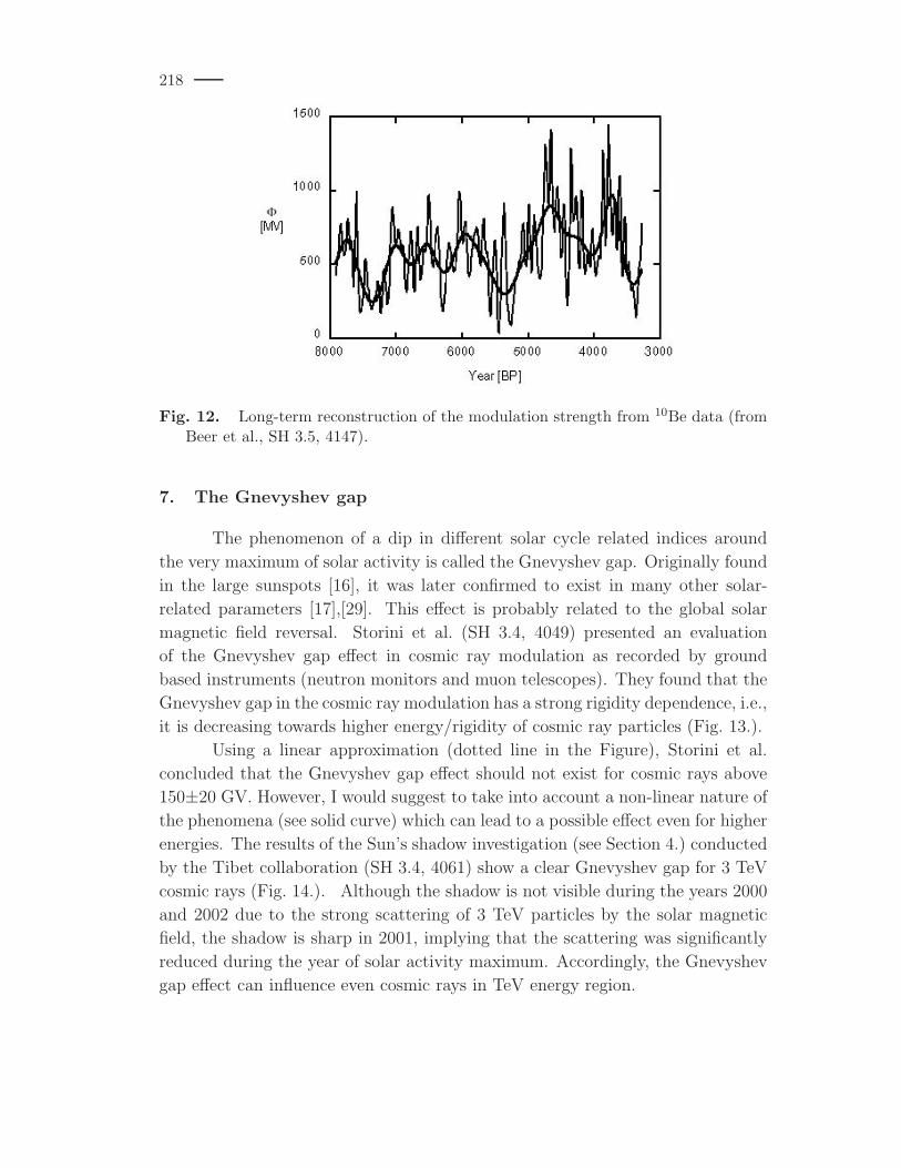
and actual data over 400-year interval validates the applied model. Inverting the

above model, Beer et al. (SH 3.5, 4147) estimated the long-term changes of the

modulation strength on multi-millennium time scale from 10Be data (Fig. 12.)

depicting its high variability and recurrent occurrence of great minima as periods

of reduced modulation.

6.1. Periods of unusual modulation

The level of heliospheric modulation strongly depends on energy/rigidity

of cosmic rays, leading to quite a different level of modulation, e.g., for different

neutron monitors: from few percent for equatorial up to 30 % for polar stations.

It is also in the anti-phase relation to the solar cycle. However, during 1970s,

the so-called mini-cycle in CR flux has occurred [36],[33],[34],[37], when the mod-

ulation was very unusual. It was rigidity independent, i.e. data from different

CR detectors depicted the same degree of modulation in the broad range of CR

rigidities (see, e.g., Fig. 2 in Ahluwalia SH 3.4, 4035 or Fig. 1 in Storini et al.,

SH 3.4, 4095). This episode forms a puzzle for the modulation theory. It can

be related either to increased λ⊥ or may appear due to an unusual heliospheric

structure [4] or may imply an unaccounted mechanism like electric drift suggested

by Ahluwalia (SH 3.4, 4035). It is also an open question if such a peculiarity is a

repetitive feature (Storini et al., SH 3.4, 4095).

Using data from ionisation chamber measurements [24] as well as 10Be

content in Greenland ice, McCracken, Beer & McDonald (SH 3.4, 4031) and

McCracken & Heikkila (SH 3.4, 4117) suggested that anomalously high flux of

lower (<1 GeV) CR was registered during the 19 cycle minimum (1954–1955).

217

0

100

200

R g

a)

0

5

10

15

Fo ,

1014

Wb

b)

0

500

1000

Φ, M

V

c)

3.5

4

4.5

5

Nst

, 105 c

nts

/h

d)

0.2

0.4

0.6

0.8

1

1.2

1.4

1.6

1600 1700 1800 1900 2000

10B

e, 1

04 ato

m/g

-700

-500

-300

-100

100

30010

Be,

pro

mill

ea)

Fig. 11. Long-term cosmic ray reconstruction (from Usoskin et al., SH 3.4, 4041).a) Group sunspot numbers [18]; b) Calculated annual open solar magnetic flux[28]; c) Calculated modulation potential; d) Calculated (solid curve) and actuallymeasured (grey curve) count rate of a polar neutron monitor; e) Calculated (greycurve) and actual annual 10Be content in Greenland ice (dotted curve, [5]). Opencircles represent the 8-year averaged 10Be data from Antarctica [3].

218

Fig. 12. Long-term reconstruction of the modulation strength from 10Be data (fromBeer et al., SH 3.5, 4147).

7. The Gnevyshev gap

The phenomenon of a dip in different solar cycle related indices around

the very maximum of solar activity is called the Gnevyshev gap. Originally found

in the large sunspots [16], it was later confirmed to exist in many other solar-

related parameters [17],[29]. This effect is probably related to the global solar

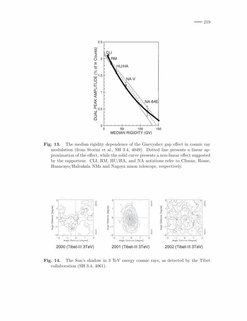
magnetic field reversal. Storini et al. (SH 3.4, 4049) presented an evaluation

of the Gnevyshev gap effect in cosmic ray modulation as recorded by ground

based instruments (neutron monitors and muon telescopes). They found that the

Gnevyshev gap in the cosmic ray modulation has a strong rigidity dependence, i.e.,

it is decreasing towards higher energy/rigidity of cosmic ray particles (Fig. 13.).

Using a linear approximation (dotted line in the Figure), Storini et al.

concluded that the Gnevyshev gap effect should not exist for cosmic rays above

150±20 GV. However, I would suggest to take into account a non-linear nature of

the phenomena (see solid curve) which can lead to a possible effect even for higher

energies. The results of the Sun’s shadow investigation (see Section 4.) conducted

by the Tibet collaboration (SH 3.4, 4061) show a clear Gnevyshev gap for 3 TeV

cosmic rays (Fig. 14.). Although the shadow is not visible during the years 2000

and 2002 due to the strong scattering of 3 TeV particles by the solar magnetic

field, the shadow is sharp in 2001, implying that the scattering was significantly

reduced during the year of solar activity maximum. Accordingly, the Gnevyshev

gap effect can influence even cosmic rays in TeV energy region.

219

Fig. 13. The median rigidity dependence of the Gnevyshev gap effect in cosmic raymodulation (from Storini et al., SH 3.4, 4049). Dotted line presents a linear ap-proximation of the effect, while the solid curve presents a non-linear effect suggestedby the rapporteur. CLI, RM, HU/HA, and NA notations refer to Climax, Rome,Huancayo/Haleakala NMs and Nagoya muon telescope, respectively.

Fig. 14. The Sun’s shadow in 3 TeV energy cosmic rays, as detected by the Tibetcollaboration (SH 3.4, 4061).

220

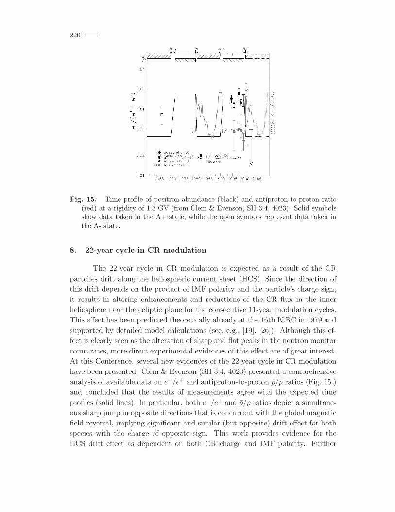
Fig. 15. Time profile of positron abundance (black) and antiproton-to-proton ratio(red) at a rigidity of 1.3 GV (from Clem & Evenson, SH 3.4, 4023). Solid symbolsshow data taken in the A+ state, while the open symbols represent data taken inthe A- state.

8. 22-year cycle in CR modulation

The 22-year cycle in CR modulation is expected as a result of the CR

partciles drift along the heliospheric current sheet (HCS). Since the direction of

this drift depends on the product of IMF polarity and the particle’s charge sign,

it results in altering enhancements and reductions of the CR flux in the inner

heliosphere near the ecliptic plane for the consecutive 11-year modulation cycles.

This effect has been predicted theoretically already at the 16th ICRC in 1979 and

supported by detailed model calculations (see, e.g., [19], [26]). Although this ef-

fect is clearly seen as the alteration of sharp and flat peaks in the neutron monitor

count rates, more direct experimental evidences of this effect are of great interest.

At this Conference, several new evidences of the 22-year cycle in CR modulation

have been presented. Clem & Evenson (SH 3.4, 4023) presented a comprehensive

analysis of available data on e−/e+ and antiproton-to-proton p/p ratios (Fig. 15.)

and concluded that the results of measurements agree with the expected time

profiles (solid lines). In particular, both e−/e+ and p/p ratios depict a simultane-

ous sharp jump in opposite directions that is concurrent with the global magnetic

field reversal, implying significant and similar (but opposite) drift effect for both

species with the charge of opposite sign. This work provides evidence for the

HCS drift effect as dependent on both CR charge and IMF polarity. Further

221

evidences for the different CR modulation during odd and even-numbered cycles

(i.e., studying only the IMF polarity effect) have been also presented (Ahluwalia,

SH 3.4, 4035; Storini et al., SH 3.4, 4095; McCracken & Heikkila, SH 3.4, 4117).

Dubey et al. (SH 3.4, 4091) reported on a shift of the diurnal anisotropy phase

towards earlier hours during qA>0 cycles. Also the amplitude of 27-day CR

variations was found to be different for odd- and even-cycles (Alania et al., SH

3.4, 4087). An interesting result was reported by Valdes-Galicia et al. (SH 3.4,

4053) on the alteration between 1.3- and 1.7-year periodicity in open/closed solar

magnetic during odd-even cycles, implying a possible 22-year cycle in the solar

magnetic flux.

9. Space weather

Space weather is related to variable radiation/magnetic conditions in the

Earths environment, and several contributions broach this topic. Belov et al.

(SH 3.6, 4213) studied a large statistics of satellite malfunctions (more than 6000

reported cases from about 300 satellites including the Soviet series of 50+ identi-

cal KOSMOS spacecrafts operating through years) in relation to different space

weather parameters. Dividing all satellites in four different groups by their orbital

parameters (altitude and inclination of the orbit), Belov et al. concluded that the

most important factor responsible for the malfunctions is the fluence of low energy

cosmic rays (both protons and electrons). They also promise to develop a method

of short-term forecast of spacecraft malfunction warnings. Meanwhile, Dorman

(SH 3.6, 4269) reviewed basic principles of space weather forecasting using CR

data.

A rigorous study of the solar particle streaming around the Earth’s mag-

netosphere has been performed by Kiraly (SH 3.5, 4057) using the long-lasting

IMP-8 measurements and taking into account variable orbital parameters of the

spacecraft. The directional distribution of the upstream particles was found to

depend strongly on the solar cycle (see Fig. 16.).

Makhmutov et al. (SH 3.6, 4233) reviewed data of electron precipitation

events recorded at a polar station during 1970-1987 and found a significant semi-

annual variation. Considering different theories, the authors concluded that the

Spring peak in electron precipitation is most likely related to Russel-McPherron

effect while the Fall broad peak is probably a superposition of Russel-McPherron,

Equinoctial and Axial effects.

222

Fig. 16. Solar cycle dependence of energetic particle streaming (IMP-8 data): largevariations of upstream ion anisotropy (from Kiraly, SH 3.4, 4057).

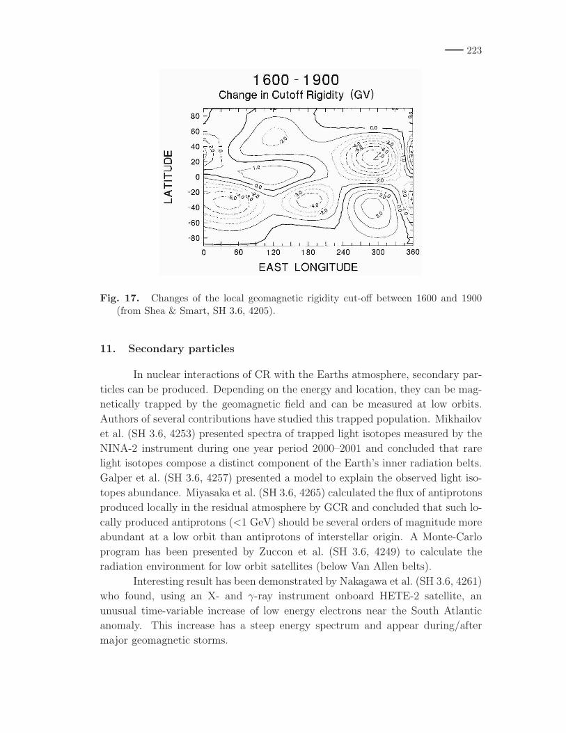
10. Geomagnetic rigidity cut-off

The geomagnetic field shields the Earth from charged particles, and this

shielding changes with the (geomagnetic) latitude: from no shielding in polar caps

where the magnetic lines are open to the very strong shielding in equatorial re-

gions. The shielding is usually considered using a simplified term of the effective

geomagnetic rigidity cut-off Pc so that CR particles with the rigidity below Pc

cannot penetrate into the atmosphere at a given location. Changes of the geo-

magnetic field (orientation and strength of the dipole) are important for studies

of CR on the long-term scale as they affect the cut-off rigidity. This issue has

been considered by Smart & Shea (SH 3.6, 4201), Shea & Smart (SH 3.6, 4205)

and Fluckiger et al. (SH 3.6, 4229). Changes in the cut-off rigidity are very large

in some regions (Fig. 17.) during the period of 1600–1900 and may reach up to

7 GV. The changes are significant even during the last century and should be

carefully taken into account.

On the other hand, it is important to take into account the rapidly chang-

ing conditions of the dynamic magnetosphere when analyzing precise data from

space borne instruments. At the Conference some results of detailed calculations

of the geomagnetic cutoff for low-orbiting satellites have been presented by Smart

et al. (SH 3.6, 4241), who succeeded reproducing the 1-min recorder radiation

doses at a Space Shuttle flight, and by Desorgher et al. (SH 3.6, 4277).

223

Fig. 17. Changes of the local geomagnetic rigidity cut-off between 1600 and 1900(from Shea & Smart, SH 3.6, 4205).

11. Secondary particles

In nuclear interactions of CR with the Earths atmosphere, secondary par-

ticles can be produced. Depending on the energy and location, they can be mag-

netically trapped by the geomagnetic field and can be measured at low orbits.

Authors of several contributions have studied this trapped population. Mikhailov

et al. (SH 3.6, 4253) presented spectra of trapped light isotopes measured by the

NINA-2 instrument during one year period 2000–2001 and concluded that rare

light isotopes compose a distinct component of the Earth’s inner radiation belts.

Galper et al. (SH 3.6, 4257) presented a model to explain the observed light iso-

topes abundance. Miyasaka et al. (SH 3.6, 4265) calculated the flux of antiprotons

produced locally in the residual atmosphere by GCR and concluded that such lo-

cally produced antiprotons (<1 GeV) should be several orders of magnitude more

abundant at a low orbit than antiprotons of interstellar origin. A Monte-Carlo

program has been presented by Zuccon et al. (SH 3.6, 4249) to calculate the

radiation environment for low orbit satellites (below Van Allen belts).

Interesting result has been demonstrated by Nakagawa et al. (SH 3.6, 4261)

who found, using an X- and γ-ray instrument onboard HETE-2 satellite, an

unusual time-variable increase of low energy electrons near the South Atlantic

anomaly. This increase has a steep energy spectrum and appear during/after

major geomagnetic storms.

224

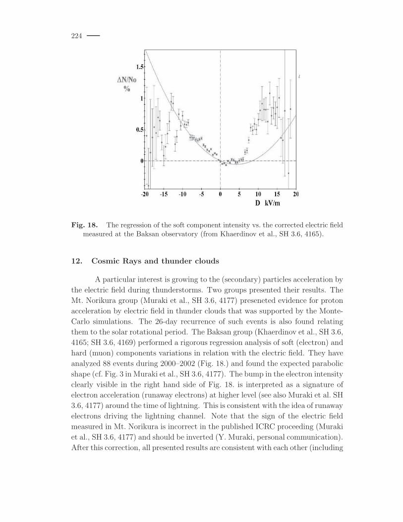
Fig. 18. The regression of the soft component intensity vs. the corrected electric fieldmeasured at the Baksan observatory (from Khaerdinov et al., SH 3.6, 4165).

12. Cosmic Rays and thunder clouds

A particular interest is growing to the (secondary) particles acceleration by

the electric field during thunderstorms. Two groups presented their results. The

Mt. Norikura group (Muraki et al., SH 3.6, 4177) preseneted evidence for proton

acceleration by electric field in thunder clouds that was supported by the Monte-

Carlo simulations. The 26-day recurrence of such events is also found relating

them to the solar rotational period. The Baksan group (Khaerdinov et al., SH 3.6,

4165; SH 3.6, 4169) performed a rigorous regression analysis of soft (electron) and

hard (muon) components variations in relation with the electric field. They have

analyzed 88 events during 2000–2002 (Fig. 18.) and found the expected parabolic

shape (cf. Fig. 3 in Muraki et al., SH 3.6, 4177). The bump in the electron intensity

clearly visible in the right hand side of Fig. 18. is interpreted as a signature of

electron acceleration (runaway electrons) at higher level (see also Muraki et al. SH

3.6, 4177) around the time of lightning. This is consistent with the idea of runaway

electrons driving the lightning channel. Note that the sign of the electric field

measured in Mt. Norikura is incorrect in the published ICRC proceeding (Muraki

et al., SH 3.6, 4177) and should be inverted (Y. Muraki, personal communication).

After this correction, all presented results are consistent with each other (including

225

also those discussed during the 27th ICRC). Ermakov and Stozhkov (SH 3.6, 4157)

described a qualitative generic model of the CR role in thunder cloud production.

According to this model, CR provide the necessary number of ions in the lower

atmosphere as well as channels for the lightning discharge.

13. Miscellanious

This section briefly discusses the results which do not fit directly the above

sections. Humble and Duldig (SH 3.6, 4197) studied asymptotic directions of a

neutron monitor in the dynamical megnetospheric model. Notable daily and

seasonal variations of the viewing directions, which are not expected in the usual

static models, were found up to 7 GV of CR rigidity. This earlier unaccounted

effects may lead to a partly spurious sederial anisotropy.

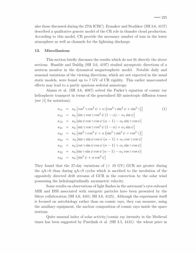
Alania et al. (SH 3.6, 4087) solved the Parker’s equation of cosmic ray

heliospheric transport in terms of the generalized 3D anisotropic diffusion tensor

(see [1] for notations):

κ11 = κ0

[cos2 γ cos2 ψ + α

(cos2 γ sin2 ψ + sin2 γ

)](1)

κ12 = κ0

[sin γ cos γ cos2 ψ (1 − α) − α1 sinψ

]

κ13 = κ0 [sinψ cos γ cosψ (α− 1) − α1 sin γ cosψ]

κ21 = κ0

[sin γ cos γ cos2 ψ (1 − α) + α1 sinψ

]

κ22 = κ0

[sin2 γ cos2 ψ + α

(sin2 γ sin2 ψ + cos2 γ

)]

κ23 = κ0 [sin γ sinψ cosψ (α− 1) + α1 cos γ cosψ]

κ31 = κ0 [cos γ sinψ cosψ (α− 1) + α1 sin γ cosψ]

κ32 = κ0 [sin γ sinψ cosψ (α− 1) − α1 cos γ cosψ]

κ33 = κ0

[sin2 ψ + α cos2 ψ

]

They found that the 27-day variations of (> 10 GV) GCR are greater during

the qA>0 than during qA<0 cycles which is ascribed to the involution of the

oppositely directed drift streams of GCR in the convection by the solar wind

possessing the heliolongitudinally asymmetric velocity.

Some results on observations of light flashes in the astronaut’s eyes onboard

MIR and ISSI associated with energetic particles have been presented by the

Sileye collaboration (SH 3.6, 4161; SH 3.6, 4125). Although the experiment itself

is focused on astrobiology rather than on cosmic rays, they can measure, using

the auxiliary equipment, the nuclear composition of cosmic rays inside the space

stations.

Quite unusual index of solar activity/cosmic ray intensity in the Medieval

times has been suggested by Pustilnik et al. (SH 3.5, 4131): the wheat price in

226

England. Due to the closed market and the risky agriculture region the wheat

market had highly nonlinear response to meteorological conditions. The wheat

prices show a good agreement with the cosmogenic isotopes in earlier times sup-

porting this idea.

14. Highlights

Many interesting results have been presented at the 28th ICRC covering

a broad field related to cosmic rays. The most interesting (subjectively selected)

new results in the Sessions reviewed here (SH 3.4–3.6) have been obtained in the

following fields (in no particular order).

• New measurements of cosmogenic isotopes. In particular, the new high

precision 14C annual data have been presented covering the Maunder and,

for the first time, Sporer minima of solar activity.

• Environmental monitoring.

• Charged particle acceleration during thunderstorms.

• Study of long-term geomagnetic cut-off rigidities.

• Measurements and models for trapped particles.

Acknowledgements

I am grateful to the Organizing Committee of the Conference for inviting me

and giving an opportunity to present this review. I thank many conferees from

whom I learned a lot during the “corridor discussions,” in addition to the formal

presentations. Special thanks to Harjit Ahluwalia, Michael Alania, Jurg Beer,

Giuliana Cini Castagnoli, Lev Dorman, Marc Duldig, John Humble, Karel Kudela,

Alexander Lidvansky, Ken McCracken, Hiroko Miyahara, Harm Moraal, Yasushi

Muraki, Lev Pustil’nik, Oscar Saavedra, Peggy Shea, Don Smart, Marisa Storini,

Yuri Stozhkov, Jose Valdec-Galicia.

References

[1] Alania, M. V., 2002, Acta Phys. Polonica B, 33, 1149

[2] Allen, D. J. et al. 2003, J. Geophys. Res., 108 (D4), TOP 3-1, DOI

10.1029/2001JD001428

[3] Bard, E., G. M. Raisbek, F. Yiou, & J. Jouzel 1997, Earth Planet. Sci. Lett.,

150, 453

227

[4] Benevolenskaya, E. E. 1998, Solar Phys., 181, 479

[5] Beer, J. et al. 1990, Nature, 347, 164

[6] Beer, J., S. Tobias, & N. Weiss 1998, Solar Phys., 181, 237

[8] Castagnoli, G., & D. Lal 1980, Radiocarbon, 22 (2), 133

[9] Dibb, J. E. 1989, J. Geophys. Res., 94, 2262

[10] McCracken, K. G., Beer, J., & McDonald, F. B. 2002, Geophys. Res. Lett.,

29(24), 2161

[11] Cliver, E. W., V. Boriakoff, & K. H. Bounar 1998, Geophys. Res. Lett., 25,

897

[12] Damon, P. E., C. J. Eastoe, & I. B. Mikheeva 1999, Radiocarbon, 41, 47

[13] Gladysheva, O. G., & G. A. M. Dreschhoff 1997, Izvestiya RAN, ser. fiz., 61,

1062 (in Russian).

[14] Gladysheva, O. G., G. E. Kocharov, G. A. Kovaltsov, I. G. Usoskin 2002,

Adv. Space Res., 29, 1707

[15] Gleeson, L. J. & W. I. Axford 1968, Astrophys. J., 154, 1011

[16] Gnevyshev, M. N. 1967, Sol. Phys., 1, 107

[17] Gnevyshev, M. N. 1977, Sol. Phys., 51, 175

[18] Hoyt, D. V. & K. Schatten 1998, Solar Phys. 179, 189

[19] Jokipii, R. & B. Thomas 1981, Astrophys. J., 243, 1115

[20] Kocharov, G. E., V. M. Ostryakov, A. N. Peristykh, V. A. Vasil’ev 1995,

Solar Phys., 159, 381

[21] Krivsky, L., & K. Pejml 1988, Astron. Inst. Czech. Acad. Sci, 75, 32

[22] Masarik, J., & J. Beer 1999 J. Geophys. Res., 104 (D10), 12099

[23] McCracken, K. G. et al. 2001a, J. Geophys. Res., 106, 21, 585

[24] Neher, H. V. 1967, J. Geophys. Res., 72, 1527

[25] Peristykh, A. N., & P. E. Damon 1998, Solar Phys., 177, 343

228

[26] Potgieter, M., & H. Moraal 1985, Astrophys. J., 294, 425

[27] Silverman, S. M. 1992, Rev. Geophys., 30, 4, 333

[28] Solanki, S. K., M. Schussler & M. Fligge 2000, Nature, 408, 445

[29] Storini, M., S. Pase, J. Sykora, M. Parisi 1997, Sol. Phys., 172, 317

[30] Stuiver, M. & T. F. Braziunas 1993, Holocene, 3, 289

[31] Stuiver, M. & T. F. Braziunas 1998, Geophys. Res. Lett., 25, 329

[32] Suess, H. E. 1955, Science, 122, 415

[33] Usoskin, I. G. et al. 1997, in: Proc. 25th Intern. Cosmic Ray Conf., Durban,

1997, v. 2, 201

[34] Usoskin, I. G. et al. 1998, J. Geophys. Res., 103 (A5), 9567

[35] Usoskin, I. G., K. Mursula, & G. A. Kovaltsov 2001, J. Geophys. Res.,

106(A8), 16039

[36] Webber, W. R., & J. A. Lockwood 1988, J. Geophys. Res., 93 (8), 8735

[37] Wibberenz, G., I. G. Richardson & H. V. Cane 2002, J. Geophys. Res.,

107(A11), SSH 5-1, DOI 10.1029/2002JA009461

[38] Zeller, E. J., & B. C. Parker 1981, Geoph. Res. Lett., 8, 895