LONG-TERM PRICE OVERREACTIONS
33
1 LONG-TERM PRICE OVERREACTIONS: ARE MARKETS INEFFICIENT? Guglielmo Maria Caporale* Brunel University London, CESifo and DIW Berlin Luis Gil-Alana University of Navarra Alex Plastun Sumy State University Revised, September 2018 Abstract This paper examines long-term price overreactions in various financial markets (commodities, US stock market and FOREX). First, a number of statistical tests are carried out for overreactions as a statistical phenomenon. Second, a trading robot approach is applied to test the profitability of two alternative strategies, one based on the classical overreaction anomaly, the other on a so-called “inertia anomaly”. Both weekly and monthly data are used. Evidence of anomalies is found predominantly in the case of weekly data. In the majority of cases strategies based on overreaction anomalies are not profitable, and therefore the latter cannot be seen as inconsistent with the EMH. Keywords: Efficient Market Hypothesis, anomaly, overreaction hypothesis, abnormal returns, contrarian strategy, trading strategy, trading robot, inertia anomaly JEL classification: G12, G17, C63 Corresponding author: Professor Guglielmo Maria Caporale, Department of Economics and Finance, Brunel University London, UB8 3PH, UK. Tel.: +44 (0)1895 266713. Fax: +44 (0)1895 269770. Email: [email protected] Comments from the Editor and an anonymous reviewer are gratefully acknowledged.
Transcript of LONG-TERM PRICE OVERREACTIONS

1
LONG-TERM PRICE OVERREACTIONS:
ARE MARKETS INEFFICIENT?
Guglielmo Maria Caporale*
Brunel University London, CESifo and DIW Berlin
Luis Gil-Alana
University of Navarra
Alex Plastun
Sumy State University
Revised, September 2018
Abstract
This paper examines long-term price overreactions in various financial markets
(commodities, US stock market and FOREX). First, a number of statistical tests are carried
out for overreactions as a statistical phenomenon. Second, a trading robot approach is
applied to test the profitability of two alternative strategies, one based on the classical
overreaction anomaly, the other on a so-called “inertia anomaly”. Both weekly and
monthly data are used. Evidence of anomalies is found predominantly in the case of
weekly data. In the majority of cases strategies based on overreaction anomalies are not
profitable, and therefore the latter cannot be seen as inconsistent with the EMH.
Keywords: Efficient Market Hypothesis, anomaly, overreaction hypothesis, abnormal
returns, contrarian strategy, trading strategy, trading robot, inertia anomaly
JEL classification: G12, G17, C63
Corresponding author: Professor Guglielmo Maria Caporale, Department of Economics
and Finance, Brunel University London, UB8 3PH, UK. Tel.: +44 (0)1895 266713. Fax:
+44 (0)1895 269770. Email: [email protected]
Comments from the Editor and an anonymous reviewer are gratefully acknowledged.
2
1. Introduction
The Efficient Market Hypothesis (EMH) is one of the central tenets of financial economics
(Fama, 1965). However, the empirical literature has provided extensive evidence of
various “anomalies”, such as fat tails, volatility clustering, long memory etc. that are
inconsistent with the EMH paradigm and suggests that it is possible to make abnormal
profits using appropriate trading strategies (Plastun, 2017). A well-known anomaly is the
so-called overreaction hypothesis, namely the idea that agents make investment decisions
giving disproportionate weight to more recent information (see De Bondt and Thaler,
1985). Clements et al. (2009) report that the overreaction anomaly has not only persisted
but in fact increased over the last twenty years. Its existence has been documented in
several studies for different markets and frequencies such as monthly, weekly or daily data
(see, e.g., Bremer and Sweeny, 1991; Clare and Thomas, 1995; Larson and Madura, 2006;
Mynhardt and Plastun, 2013; Caporale et al. 2017).
There exist a significant number of studies on market overreactions but most of them
analyse short-term price overreactions based on daily data (Atkins and Dyl, 1990; Bremer
and Sweeney, 1991; Cox and Peterson, 1994; Choi and Jayaraman, 2009) and focus only
on a single market/asset. By contrast, this paper analyses long-term overreactions and a
variety of markets and frequencies by (i) carrying out various statistical tests to establish
whether overreaction anomalies exist using both weekly and monthly data, and (ii) using a
trading robot method to examine whether they give rise to exploitable profit opportunities,
i.e. whether price overreactions are simply a statistical phenomena or can also be seen as
evidence against the EMH. The analysis is carried out for various financial markets: the
US stock market (the Dow Jones Index and 10 companies included in this index), FOREX
(10 currency pairs) and commodity markets (gold and oil). A similar investigation was
carried out by Caporale et al. (2018); however, their analysis focused on short-term (i.e.,

3
daily) overreactions, whilst the present study considers a longer horizon, namely a week or
a month.
The remainder of the paper is organised as follows. Section 2 reviews the existing
literature on the overreaction hypothesis. Section 3 describes the methodology used in this
study. Section 4 discusses the empirical results. Section 5 provides some concluding
remarks.
2. Literature Review
The seminal paper on the overreaction hypothesis is due to De Bondt and Thaler (DT,
1985), who followed the work of Kahneman and Tversky (1982), and showed that the best
(worst) performing portfolios in the NYSE over a three-year period tended to under (over)-
perform over the following three-year period. Their explanation was that significant
deviations of asset prices from their fundamental value occur because of agents’ irrational
behaviour, with recent news being given an excessive weight. DT also reported an
asymmetry in the overreaction (it is bigger for undervalued than for overvalued stocks),
and a "January effect", with a clustering of overreactions in that particular month.
Other studies include Brown, Harlow and Tinic (1988), who analysed NYSE data
for the period 1946-1983 and reached similar conclusions to DT; Ferri and Min (1996),
who confirmed the presence of overreactions using S&P 500 data for the period 1962-
1991; Larson and Madura (2003), who used NYSE data for the period 1988-1998 and also
showed the presence of overreactions. Clement et al. (2009) confirmed the original
findings of DT using CRSP data for the period 1926-1982, and also showed that the
overreaction anomaly had increased during the following twenty years.
In addition to papers analysing stock markets (Alonso and Rubio, 1990, Brailsford,
1992, Bowman and Iverson, 1998, Antoniou et. al., 2005, Mynhardt and Plastun, 2013
among others), some consider other markets such as the gold (Cutler, Poterba, and

4
Summers (1991)), or the options market (Poteshman, 2001). Finally, Conrad and Kaul
(1993) showed that the returns used in many studies (supporting the overreaction
hypothesis) are upwardly biased, and “true” returns have no relation to overreaction;
therefore this issue is still unresolved.
The other aspect of the overreaction hypothesis is its practical implementation, i.e.
the possibility of obtaining extra profits by exploiting this anomaly. Jegadeesh and Titman
(1993) and Lehmann (1990) found that a strategy based on overreactions can indeed
generate abnormal profits. Baytas and Cakiki (1999) also tested a trading strategy based on
the overreaction hypothesis, and showed that contrarian portfolios on the long-term
horizons can generate significant profits.
The most recent and thorough investigation is due to Caporale et al. (2018), who
analyse different financial markets (FOREX, stock and commodity) using the same
approach as in the present study. That study shows that a strategy based on counter-
movements after overreactions does not generate profits in the FOREX and the commodity
markets, but it is profitable in the case of the US stock market. Also, it detects a brand new
anomaly based on the overreaction hypothesis, i.e. an “inertia” anomaly (after an
overreaction day prices tend to move in the same direction for some time). Here we extend
the analysis by considering long-term overreactions and the possibility of making extra
profits over weekly and monthly intervals. The variety of assets and markets (FOREX,
stock market, commodities) as well as of time frequencies (weekly, monthly) considered in
this study can help to address issues such as robustness, data snooping, data mining etc.
Moreover, since according to the Adaptive Markets Hypothesis (Lo, 2004) financial
markets evolve and anomalies may disappear during this process, it is important to include
the most recent data as we do.

5
3. Data and Methodology
We analyse the following weekly and monthly series: for the US stock market, the Dow
Jones index and stocks of two companies included in this index (Microsoft and Boeing -
for the trading robot analysis we also add Alcoa, AIG, Walt Disney, General Electric,
Home Depot, IBM, Intel, Exxon Mobil); for the FOREX, EURUSD, USDCHF and
AUDUSD (for the trading robot analysis also USDJPY, USDCAD, GBPJPY, GBPUSD,
EURJPY, GBPCHF, EURGBP); for commodities, gold and oil (only gold for the trading
robot analysis owing to data unavailability). The choice of assets is based on their liquidity,
trading volume, data availability, and extent of use. The sample covers the period from
January 2002 till the end of December 2016, and for the trading robot analysis the period is
2002-2014 for the FOREX and 2006-2014 for the US stock market and commodity market.
These dates are selected on the basis of data availability (especially for the purpose of
trading robot analysis) and to include the most recent data since markets can evolve as
stressed by the Adaptive Market Hypothesis.
3.1 Student’s t-tests
First we carry out Student’s t-tests to confirm (reject) the presence of anomalies after
overreactions. To provide additional evidence we also conduct ANOVA analysis, and
carry out Mann–Whitney U tests not relying on the normality assumption.
To identify anomalies we run multiple regressions including a dummy variable:
Yt = a0 + a1 D1t + εt (1)
where Yt – volatility on the period t;
a0– mean volatility for a normal day (the day when there was no volatility
explosion);
a1 – dummy coefficient;

6
D1t - a dummy variable for a specific data group, equal to 1 when the data belong to
a day of volatility explosion, and equal to 0 when they do not;
εt – Random error term for period t.
The size, sign and statistical significance of the dummy coefficient provide
information about possible anomalies.
Then we apply the trading robot approach to establish whether the detected
anomalies create exploitable profit opportunities. According to the classical overreaction
hypothesis, an overreaction should be followed by a correction, i.e. price counter-
movements, and this should be bigger than after normal days. If one day is not enough for
the market to incorporate new information, i.e. to overreact, then after one-day abnormal
price changes one can expect movements in the direction of the overreaction bigger than
after normal days.
The two hypotheses to be tested are therefore:
H1: Counter-reactions after overreactions differ from those after normal periods.
H2: Price movements after overreactions in the direction of the overreaction differ
from such movements after normal periods.
The null hypothesis is in both cases that the data after normal and overreaction
periods belong to the same population.
As already mentioned, we focus on long-term overreactions, so the period of
analysis is one week or one month. The parameters characterising price behaviour over
such a time interval are maximum, minimum, open and close prices. In most studies price
movements are measured as the difference between the open and close price. In our
opinion the weekly (monthly) return, i.e. the difference between the maximum and
minimum prices during the week (month), is more appropriate. This is calculated as:
,%100Low
)LowHigh(R
i
iii
(2)

7
where iR is the % weekly (monthly) return, iHigh is the maximum price, and iLow is the
minimum price for week (month) і.
We consider three definitions of “overreaction”:
1) when the current weekly (monthly) return exceeds the average plus one
standard deviation
,)R(R nni (3)
where nR is the average size of weekly (monthly) returns for period n
,n/RRn
1iin
(4)
and n is the standard deviation of weekly (monthly) returns for period n
.)RR(n
1 n
1i
2in
(5)
2) when the current weekly (monthly) return exceeds the average plus two standard
deviations, i.e.,
)2R(R nni . (6)
3) when the current weekly (monthly) return exceeds the average plus three
standard deviations, i.e.,
)3R(R nni .
(7)
The next step is to determine the size of the price movement during the following
week (month). For Hypothesis 1 (the counter-reaction or counter-movement assumption),
we measure it as the difference between the next period’s open price and the maximum
deviation from it in the opposite direction to the price movement in the overreaction
period.
If the price increased, then the size of the counter-reaction is calculated as:

8
1i
1i1i1i
Low
)LowOpen(%100cR
,
(8)
where 1icR is the counter-reaction size, and liOpen is the next period’s open price.
If the price decreased, then the corresponding definition is:
1i
1i1i1i
Open
)OpenHigh(%100сR
.
(9)
In the case of Hypothesis 2 (movement in the direction of the overreaction), either
equation (9) or (8) is used depending on whether the price has increased or decreased.
Two data sets (with 1icR values) are then constructed, including the size of price
movements after normal and abnormal price changes respectively. The first data set
consists of 1icR values after period with abnormal price changes. The second contains
1icR values after a period with normal price changes. The null hypothesis to be tested is
that they are both drawn from the same population.
3.2 Trading Robot Analysis
The trading robot approach considers the long-term overreactions from a trader’s
viewpoint, i.e. whether it is possible to make abnormal profits by exploiting the
overreaction anomaly, and simulates the actions of a trader using an algorithm representing
a trading strategy. This is a programme in the MetaTrader terminal that has been developed
in MetaQuotes Language 4 (MQL4) and used for the automation of analytical and trading
processes. Trading robots (called experts in MetaTrader) allow to analyse price data and
manage trading activities on the basis of the signals received.
MetaQuotes Language 4 is the language for programming trade strategies built in
the client terminal. The syntax of MQL4 is quite similar to that of the C language. It allows
to programme trading robots that automate trade processes and is ideally suited to the
9
implementation of trading strategies. The terminal also allows to check the efficiency of
trading robots using historical data. These are saved in the MetaTrader terminal as bars and
represent records appearing as TOHLCV (HST format). The trading terminal allows to test
experts by various methods. By selecting smaller periods it is possible to see price
fluctuations within bars, i.e., price changes will be reproduced more precisely. For
example, when an expert is tested on one-hour data, price changes for a bar can be
modelled using one-minute data. The price history stored in the client terminal includes
only Bid prices. In order to model Ask prices, the strategy tester uses the current spread at
the beginning of testing. However, a user can set a custom spread for testing in the
"Spread", thereby approximating better actual price movements.
We examine two trading strategies:
- Strategy 1 (based on H1): This is based on the classical overreaction anomaly,
i.e. the presence of abnormal counter-reactions after the overreaction period. The
algorithm is constructed as follows: at the end of the overreaction period financial
assets are sold or bought depending on whether abnormal price increases or
decreased respectively have occurred. An open position is closed if a target profit
value is reached or at the end of the following period (for details of how the target
profit value is defined see below).
- Strategy 2 (based on H2): This is based on the non-classical overreaction
anomaly, i.e. the presence the abnormal price movements in the direction of the
overreaction in the following period. The algorithm is built as follows: at the end of
the overreaction period financial assets are bought or sold depending on whether
abnormal price increases or decreases respectively have occurred. Again, an open
position is closed if a target profit value is reached or at the end of the following
period.

10
The results of the trading strategy testing and some key data are presented in the
"Report" in Appendix A. The most important indicators given in the “Report” are:
- Total net profit: this is the difference between "Gross profit" and "Gross loss"
measured in US dollars. We used marginal trading with the leverage 1:100,
therefore it is necessary to invest $1000 to make the profit mentioned in the
Trading Report. The annual return is defined as Total net profit/100, so, for
instance, an annual total net profit of $100 represents a 10% annual return on
the investment;
- Profit trades: % of successful trades in total trades;
- Expected payoff: the mathematical expectation of a win. This parameter
represents the average profit/loss per trade. It is also the expected
profitability/unprofitability of the next trade;
- Total trades: total amount of trade positions;
- Bars in test: the number of past observations modelled in bars during testing.
The results are summarised in the “Graph” section of the “Report”: this represents
the account balance and general account status considering open positions. The “Report”
also provides full information on all the simulated transactions and their financial results.
The following parameters affect the profitability of the trading strategies (the next section
explains how they are set):
- Criterion for overreaction (symbol: sigma_dz): the number of standard
deviations added to the mean to form the standard period interval;
- Period of averaging (period_dz): the size of the data set used to calculate base
mean and standard deviation;
- Time in position (time_val): how long the opened position has to be held.
We carry out t-tests to examine whether the results we obtain are statistically
different from the random ones. We chose this approach because the sample size is usually

11
less than 100. A t-test compares the means from two samples to see whether they come
from the same population. In our case the first is the average profit/loss factor of one trade
applying the trading strategy, and the second is equal to zero because random trading
(without transaction costs) should generate zero profit.
The null hypothesis (H0) is that the mean is the same in both samples, and the
alternative (H1) that it is not. The computed values of the t-test are compared with the
critical one at the 5% significance level. Failure to reject H0 implies that there are no
advantages from exploiting the trading strategy being considered, whilst a rejection
suggests that the adopted strategy can generate abnormal profits.
Example of the t-test results are reported in Table 1. As can be seen the results
obtained are not differing from the random ones.
Table 1: t-test for the trading simulation results for Strategy 1 (case of
EURUSD, testing period 2001-2014)*
Parameter Value
Number of the trades 96
Total profit -1331.03
Average profit per trade -13.86
Standard deviation 192,27
t-test -0.70
z critical (0,95) 1.78
Null hypothesis Accepted
* For data sources see Appendix A
As can be seen, H0 cannot be rejected, which implies that the trading simulation
results are not statistically different from the random ones and therefore this trading
strategy is not effective and there is no exploitable profit opportunity.
4. Empirical Results
The first step is to set the basic overreaction parameters/criterions by choosing the number
of standard deviations (sigma_dz) to be added to the average to form the “standard” period

12
interval for price fluctuations and the averaging period to calculate the mean and the
standard deviation (symbol: period_dz).
For this purpose we used the Dow Jones Index data for the time period 1991-2014.
The number of abnormal returns detected in the period 1991-2014 is reported in Table 2
(for weekly data) and Table 3 (for monthly data).
Table 2: Number of abnormal returns detections in Dow-Jones index during 1991-
2014 (weekly data)
Period_dz 3 5 10 20 30
Indicator Number % Number % Number % Number % Number %
Overall 1241 100 1239 100 1233 100 1223 100 1213 100
Number of abnormal
returns (criterion
=mean+sigma_dz) 251 20 239 19 206 17 198 16 198 16
Number of abnormal
returns (criterion=
mean+2*sigma_dz) 0 0 0 0 56 5 65 5 69 6
Number of abnormal
returns (criterion =
mean+3*sigma_dz) 0 0 0 0 0 0 13 1 19 2
Table 3: Number of abnormal returns detections in Dow-Jones index during 1991-
2014 (monthly data)
Period_dz 3 5 10 20 30
Indicator Number % Number % Number % Number % Number %
Overall 285 100 283 100 278 100 268 100 258 100
Number of abnormal
returns (criterion
=mean+sigma_dz) 56 20 52 18 45 16 42 15 44 15
Number of abnormal
returns (criterion=
mean+2*sigma_dz) 0 0 0 0 16 6 20 7 22 8
Number of abnormal
returns (criterion =
mean+3*sigma_dz) 0 0 0 0 0 0 4 1 6 2
As can be seen from the above tables, both parameters (averaging period and
number of standard deviations added to the mean) affect the number of detected anomalies.
Changes in the averaging period have relatively small effect on the number of detected
anomalies (the difference between the results when the period considered is 5 and 30
respectively is less than 20%). By contrast, each additional standard deviation significantly

13
decreases the number of observed abnormal returns. Therefore 2-4% of the full sample (the
number of abnormal returns in the case of 3 sigmas) is not sufficiently representative to
draw conclusions. To investigate whether sigma_dz equal to 1 is most appropriate we carry
out t-tests of long-term counter-reactions for the Dow Jones index over the period 1991-
2014 (see Tables 4 and 5 for weekly and monthly data respectively). As can be seen, the
anomaly is most easily detected in the case of sigma_dz= 1 (the t-stat is the biggest), and
therefore we set sigma_dz equal to 1.
Table 4: T-test of the counter-reactions after the overreaction for the Dow-Jones
index during 1991-2014 (weekly data) for the different values of sigma_dz parameter
case of period_dz=30 Number of standard
deviations 1 2 3
abnormal normal abnormal normal abnormal normal
Number of matches 198 1015 69 1144 19 1194
Mean 2,36% 1,74% 2,77% 1,78% 3,57% 1,81%
Standard deviation 2,22% 1,52% 2,43% 1,59% 3,15% 1,62%
t-criterion 3,91 3,38 2,44
t-critical (р=0.95) 1,96 1,96 1,96
Null hypothesis rejected rejected rejected
Table 5: T-test of the counter-reactions after the overreaction for the Dow-Jones
index during 1991-2014 (monthly data) for the different values of sigma_dz
parameter case of period_dz=30 Number of standard
deviations 1 2 3
abnormal normal abnormal normal abnormal normal
Number of matches 44 214 22 236 6 252
Mean 4,39% 3,22% 4,25% 3,34% 7,97% 3,31%
Standard deviation 4,09% 2,83% 4,37% 2,96% 6,78% 2,90%
t-criterion 1,90 0,98 1,68
t-critical (р=0.95) 1,96 1,96 1,96
Null hypothesis accepted accepted accepted
Student’s t –tests of long-term counter-reactions for the Dow Jones index over the
period 1991-2014 (Tables 6 and 7 for weekly and monthly data respectively) suggest that

14
the optimal averaging period is 30, their corresponding t-statistics being significantly
higher than for other averaging periods.
Table 6: T-test of the counter-reactions after the overreaction for the Dow-Jones
index during 1991-2014 (weekly data) for the different averaging periods case of
sigma_dz=1
Period_dz 3 5 10 20 30
abnormal normal abnormal normal abnormal normal abnormal normal abnormal normal
Number of
matches 251 990
239 1000 206 1027 198 1025 198 1015
Mean 2,05% 1,78% 2,05% 1,78% 2,11% 1,78% 2,24% 1,76% 2,36% 1,74%
Standard
deviation 1,78% 1,62%
1,82% 1,61% 1,89% 1,60% 1,94% 1,59% 2,22% 1,52%
t-criterion 2,45 2,26 2,50 3,51 3,91
t-critical
(р=0.95) 1,96 1,96 1,96 1,96 1,96
Null
hypothesis rejected rejected rejected rejected rejected
Table 7: T-test of the counter-reactions after the overreaction for the Dow-Jones
index during 1991-2014 (monthly data) for the different averaging periods case of
sigma_dz=1
Period_dz 3 5 10 20 30
abnormal normal abnormal normal abnormal normal abnormal normal abnormal normal
Number of
matches 56 229 52 230 45 233 42 226 44 214
Mean 3,59% 3,40% 3,51% 3,42% 3,73% 3,37% 3,80% 3,32% 4,39% 3,22%
Standard
deviation 3,37% 2,94% 3,41% 2,95% 3,66% 2,93% 3,80% 2,90% 4,09% 2,83%
t-criterion 0,40 0,20 0,66 0,82 1,90
t-critical
(р=0.95) 1,96 1,96 1,96 1,96 1,96
Null
hypothesis accepted accepted accepted accepted accepted
Therefore the key parameters for the tests of long-term overreaction in different
financial markets analysis are set as follows: the period_dz (averaging period) is set equal
to 30 and sigma_dz (the number of standard deviations added to mean used as a criterion
of overreaction) equal to 1.
The results for H1 are presented in Appendix B (weekly data) and C (monthly data)
and are summarised in Tables 8-9.

15
Table 8: Statistical tests results: case of Hypothesis 1 (weekly data)*
Financial market FOREX Commodities US stock market
Financial asset EURUSD USDCHF AUDUSD Gold Oil Boeing Microsoft
T-test - - - + + - -
ANOVA - + + + + + -
Mann–Whitney U test - - - + + + -
Regression analysis
with dummy variables - + + + + + -
* ”+” – anomaly confirmed, “-” - anomaly not confirmed.
As can be seen in the case of weekly data strong statistical evidence in favour of the
overreaction anomaly can be found for both Gold and Oil prices, and to some extent for the
US stock market (in the case of Boeing) and the FOREX (in the case of USDCHF and
AUDUSD).
Table 9: Statistical tests results: case of Hypothesis 1 (monthly data)*
Financial market FOREX Commodities US stock market
Financial asset EURUSD USDCHF AUDUSD Gold Oil Boeing Microsoft
T-test - - - - - - -
ANOVA - + - + - - -
Mann–Whitney U test + - - - - - -
Regression analysis
with dummy variables - + - + - - -
* ”+” – anomaly confirmed, “-” - anomaly not confirmed.
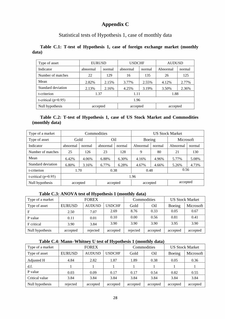
The results for the monthly data are significantly different from those for the
weekly ones. The evidence of anomalies almost completely disappears, except for
EURUSD and USDCHF (in the case of the FOREX) and Gold (in the case of
commodities).
Overall, it appears that in the case of H1 weekly data provides the strongest
evidence for the classical short-term counter-movement after an overreaction day, which is
most noticeable in the case of commodities.

16
The results for H2 are presented in Appendix D (weekly data) and E (monthly data)
and are summarised in Tables 10-11.
Table 10: Statistical tests results: case of Hypothesis 2 (weekly data)*
Financial market FOREX Commodities US stock market
Financial asset EURUSD USDCHF AUDUSD Gold Oil Boeing Microsoft
T-test + - + - + - +
ANOVA + + + + + - +
Mann–Whitney U test + - + - + - +
Regression analysis
with dummy variables + + + + + - +
* ”+” – anomaly confirmed, “-” - anomaly not confirmed.
Hypothesis 2 is not rejected in many cases with weekly data. We find very strong
evidence in favour of an “inertia anomaly” (prices tend to move in the direction of the
overreaction in the following period). This applies to EURUSD and AUDUSD, Oil and
Microsoft data, and represents evidence of market inefficiency caused by overreactions.
Table 11: Statistical tests results: case of Hypothesis 2 (monthly data)*
Financial market FOREX Commodities US stock market
Financial asset EURUSD USDCHF AUDUSD Gold Oil Boeing Microsoft
T-test - - - + + - -
ANOVA - + + + + - +
Mann–Whitney U test - - + + + - -
Regression analysis with
dummy variables - + + + + - +
* ”+” – anomaly confirmed, “-” - anomaly not confirmed.
The results for the monthly data again are significantly differing from those for the
weekly ones. Evidence in favour of the inertia anomaly is present for commodities and
only for AUSUSD in the FOREX.
Overall the results from testing Hypothesis 2 suggest that the weekly frequency is
the most appropriate to detect the inertia anomaly. The commodity market again look like
the most inefficient among those analysed.

17
The general conclusion from the statistical tests are as follows: anomalies are
generally detected using weekly but not monthly data; the commodity markets are the most
affected by the overreaction anomalies; the results for the FOREX and US stock markets
are mixed.
Next, we analyse whether these anomalies give rise to exploitable profit
opportunities. If they do not, we conclude that they do not represent evidence inconsistent
with the EMH. We expand the list of assets in order to provide more extensive results. The
complete list of assets includes: FOREX (EURUSD, USDCHF, AUDUSD, USDJPY,
USDCAD, GBPJPY, GBPUSD, EURJPY, GBPCHF, EURGBP), US stock market (Alcoa,
AIG, Boeing Company, Walt Disney, General Electric, Home Depot, IBM, Intel,
Microsoft, Exxon Mobil), commodity (Gold).
The parameters of the trading strategies 1 and 2 are set as follows:
- Period_dz = 30 (see above for an explanation);
- Time_val = week (see above);
- Sigma_dz=1 (see above).
The results of the trading robot analysis are presented in Table 12 (Strategy 1) and
Table 13 (Strategy 2). The testing periods are as follows FOREX: 2001-2014; US stock
market: 2006-2014; Commodities: 2006-2014.
Table 12: Trading results for Strategy 1
Asset Total
trades
Succesfull
trades, %
Profit,
USD Return
Annual
return
t-test
FOREX
EURUSD 108 63% -1584 -158,4% -11,3% Accepted
USDCHF 112 63% -1815 -181,5% -13,0% Accepted
AUDUSD 114 66% -1 690 -169,0% -12,1% Accepted
USDJPY 116 69% 1 662 166,2% 11,9% Rejected
USDCAD 118 66% -2 121 -212,1% -15,2% Accepted
GBPJPY 111 71% 3 541 354,1% 25,3% Rejected
GBPUSD 116 68% -135 -13,5% -1,0% Accepted
EURJPY 107 64% -1 829 -182,9% -13,1% Accepted

18
GBPCHF 106 74% 3 721 372,1% 26,6% Rejected
EURGBP 118 71% 169 16,9% 1,2% Accepted
US stock market
Alcoa 64 63% -2280 -228,0% -25,3% Accepted
AIG 64 67% 480 48,0% 5,3% Accepted
Boeing Company 87 71% 3290 329,0% 36,6% Rejected
Walt Disney 63 70% -289 -28,9% -3,2% Accepted
General electric 67 64% -39 -3,9% -0,4% Accepted
Home Depot 79 64% 290 29,0% 3,2% Accepted
IBM 65 63% -3090 -309,0% -34,3% Accepted
Intel 70 54% -1055 -105,5% -11,7% Accepted
Microsoft 74 66% 430 43,0% 4,8% Accepted
Exxon Mobil 72 67% 773 77,3% 8,6% Accepted
Commodities
Gold 78 64,0% -2091 -209,1% -23,2% Accepted
Strategy 1, based on the classical overreaction hypothesis, trades on counter-
reactions after periods of abnormal price dynamics. In general, it is unprofitable in the case
of the FOREX (7 pairs out of 10 produce negative or statistically insignificant results) and
commodity markets (in the case of Gold). For the US stock market the results are mixed
(50% of profitable assets), but in general this anomaly does not seem to be exploitable. The
assets to be traded on the basis of the classical overreaction hypothesis with weekly data
are therefore: GBPCHF (ROI=27% per year), GBPJPY (25%), USDJPY (12%) and
Boeing (36.6%). Although as previously shown a non-rejection of the null does not
necessarily mean that there exist profit opportunities, it appears that it does mean a higher
chance of profitable trading.
Table 13: Trading results for Strategy 2
Asset Total
trades
Succesfull
trades, %
Profit,
USD Return
Annual
return
t-test
FOREX
EURUSD 112 58% 848 84,8% 6,1% Rejected
USDCHF 119 57% 690 69,0% 4,9% Rejected
AUDUSD 117 56% 416 41,6% 3,0% Accepted
USDJPY 116 50% -479 -47,9% -3,4% Accepted
USDCAD 117 58% 1 829 182,9% 13,1% Rejected
GBPJPY 114 47% -6 766 -676,6% -48,3% Accepted
GBPUSD 116 53% -566 -56,6% -4,0% Accepted
EURJPY 107 58% 476 47,6% 3,4% Accepted
19
GBPCHF 106 48% -2 991 -299,1% -21,4% Accepted
EURGBP 118 49% -2 609 -260,9% -18,6% Accepted
US stock market
Alcoa 68 51% 877 87,7% 9,7% Rejected
AIG 65 60% 2390 239,0% 26,6% Rejected
Boeing Company 87 44% -2470 -247,0% -27,4% Accepted
Walt Disney 62 47% -1475 -147,5% -16,4% Accepted
General electric 69 51% 410 41,0% 4,6% Accepted
Home Depot 79 47% -1557 -155,7% -17,3% Accepted
IBM 65 38% -9236 -923,6% -102,6% Accepted
Intel 70 50% -36,4 -3,6% -0,4% Accepted
Microsoft 74 40% -1814 -181,4% -20,2% Accepted
Exxon Mobil 71 50% -1711 -171,1% -19,0% Accepted
Commodities
Gold 78 58,0% 1011 101,1% 11,2% Rejected
Strategy 2, based on the so-called “inertia anomaly”, trades on price movements in
the direction of the overreaction in the following period. In general it is unprofitable for the
US stock market (7 assets out of the 10 analysed produce negative results), whilst the
results are mixed for the FOREX (there are 50% of profitable assets, but only 3 of the 5
profitable assets pass the t-test on randomness). There is evidence of profit opportunities in
the commodity markets. The assets to be traded on the basis of the inertia anomaly with
weekly data are therefore: USDCAD (ROI=13% per year), USDCHF (5%), EURUSD
(6%), AIG (27%), Alcoa (10%) and Gold (11%).
5. Conclusions
This paper examines long-term price overreactions in various financial markets
(commodities, US stock market and FOREX). It addresses the issue of whether they should
be seen simply as a statistical phenomenon or instead as anomalies giving rise to
exploitable profit opportunities, only the latter being inconsistent with the EMH paradigm.
The analysis is conducted in two steps. First, a number of statistical tests are carried out for
overreactions as a statistical phenomenon. Second, a trading robot approach is applied to
test the profitability of two alternative strategies, one based on the classical overreaction
20
anomaly (H1: counter-reactions after overreactions differ from those after normal periods),
the other on an “inertia” anomaly (H2: price movements after overreactions in the same
direction of the overreaction differ from those after normal periods). Both weekly and
monthly data are used. Evidence of anomalies is found predominantly in the case of
weekly data.
More specifically, H1 cannot be rejected for the US stock market and commodity
markets when the averaging period is 30, whilst it is rejected for the FOREX. The results
for H2 are more mixed and provide evidence of an “inertia” anomaly in the commodity
market and for some assets in the US stock market and FOREX. The trading robot analysis
shows that in general strategies based on the overreaction anomalies are not profitable, and
therefore the latter cannot be seen as inconsistent with the EMH. However, in some cases
abnormal profits can be made; in particular this is true of (i) GBPCHF (ROI=27% per
year), GBPJPY (25%), Boeing (36%), ExxonMobil (8.6%) in the case of the classical
overreaction hypothesis and weekly data, and (ii) USDCAD (13%), USDCHF (5%),
EURUSD (6%), AIG (27%), Alcoa (10%) and Gold (11%) in the case of the inertia
anomaly and also with weekly data.
A comparison between these results and the daily ones reported in Caporale et al.
(2017) suggests that the classic overreaction anomaly (H1) occurs at both short- and long-
term intervals in the case of the US stock market and commodity markets. The results for
the FOREX are mixed at both intervals, but mostly suggest no contrarian movements after
overreactions. The findings concerning the “inertia” anomaly (H2) are more stable and
consistent: it is detected for the commodity markets and US stock market at both short- and
long-term horizons. As for the FOREX, there is a short- but not a long-term anomaly in
most cases. The trading results imply that there is no single profitable strategy: the findings
are quite sensitive to the specific asset being considered, and therefore it is necessary to
investigate case by case whether it is possible to earn abnormal profits by exploiting the

21
classical overreaction and/or inertia anomaly. Future research will extend the analysis
focusing in particular on unusually low returns.

22
References
Alonso, A. and G. Rubio, (1990), Overreaction in the Spanish Equity Market. Journal of
Banking and Finance 14, 469–481.
Antoniou, A., E. C. Galariotis and S. I. Spyrou, (2005), Contrarian Profits and the
Overreaction Hypothesis: The Case of the Athens Stock Exchange. European Financial
Management 11, 71–98.
Atkins, A.B. and E.A. Dyl, (1990), Price Reversals, Bid-Ask Spreads, and Market
Efficiency. Journal of Financial and Quantitative Analysis 25, 535 – 547.
Baytas, A. and N.Cakici, (1999), Do markets overreact: international evidence. Journal of
Banking and Finance 23, 1121-1144.
Bowman, R. G. and D. Iverson, (1998), Short-run Over-reaction in the New Zealand Stock
Market. Pacific-Basin Finance Journal 6, 475–491.
Brailsford, T., (1992), A Test for the Winner–loser Anomaly in the Australian Equity
Market: 1958–1987. Journal of Business Finance and Accounting 19, 225–241.
Bremer, M. and R. J. Sweeney, (1991), The reversal of large stock price decreases. Journal
of Finance 46, 747-754.
Brown, K. C., W.V. Harlow and S. M. Tinic, (1988), Risk Aversion, Uncertain
Information, and Market Efficiency. Journal of Financial Economics 22, 355 - 385.
Caporale, G. M., L. Gil-Alana, and A. Plastun, (2018), Short-term Price Overreactions:
Identification, Testing, Exploitation. Computational Economics 51(4), 913-940.
Choi, H.-S. and N. Jayaraman, (2009), Is reversal of large stock-price declines caused by
overreaction or information asymmetry: Evidence from stock and option markets. Journal
of Future Markets 29, 348–376.
Clare, A. and S. Thomas, (1995), The Overreaction Hypothesis and the UK Stock Market.
Journal of Business Finance and Accounting 22, 961–973.
Clements, A., M. Drew, E. Reedman and M. Veeraraghavan, (2009), The Death of the
Overreaction Anomaly? A Multifactor Explanation of Contrarian Returns. Investment
Management and Financial Innovations 6, 76-85.
Conrad, J. and G. Kaul, (1993), Long-term market overreaction or biases in computed
return? Journal of Finance 48, 1-38.
Cox, D. R. and D. R. Peterson, (1994), Stock Returns Following Large One-Day Declines:
Evidence on Short-Term Reversals and Longer-Term Performance. Journal of Finance 49,
255-267.
Cutler, D., J. Poterba, and L. Summers, (1991), Speculative dynamics. Review of
Economics Studies 58, 529–546.

23
De Bondt W. and R. Thaler, (1985), Does the Stock Market Overreact?. Journal of Finance
40, 793-808.
Fama, E. F., (1965), The Behavior of Stock-Market Prices. The Journal of Business 38, 34-
105.
Ferri, M., G. and C. Min, (1996), Evidence that the Stock Market Overreacts and Adjusts.
The Journal of Portfolio Management 22, 71-76.
Jegadeesh, N. and S. Titman, (1993), Returns to Buying Winners and Selling Losers:
Implications for Stock Market Efficiency. The Journal of Finance 48, 65-91.
Kahneman, D. and A. Tversky, (1982), The psychology of preferences. Scientific
American246, 160-173.
Larson, S. and J. Madura, (2003), What Drives Stock Price Behavior Following Extreme
One-Day Returns. Journal of Financial Research Southern Finance Association26, 113-
127.
Lehmann, B., (1990), Fads, Martingales, and Market Efficiency. Quarterly Journal of
Economics 105, 1-28.
Lo, A., (2004), The Adaptive Markets Hypothesis: Market Efficiency from an
Evolutionary Perspective. Journal of Portfolio Management 30(5), 15–29.
Mendenhall, W., R. J. Beaver and B. M. Beaver, (2003), Introduction to Probability and
Statistics, 11th edn, Brooks / Cole, Pacific Grove.
Mynhardt, R. H. and A. Plastun, (2013), The Overreaction Hypothesis: The case of
Ukrainian stock market. Corporate Ownership and Control 11, 406-423.
Plastun, Oleksiy, Chapter 24: Behavioral Finance Market Hypotheses (2017). Financial
Behavior: Players, Services, Products, and Markets. H. Kent Baker, Greg Filbeck, and
Victor Ricciardi, editors, 439-459, New York, NY: Oxford University Press, 2017.
Poteshman, A., (2001), Underreaction, overreaction and increasing misreaction to
information in the options market. Journal of Finance 56, 851–876.

24
Appendix A
Example of strategy tester report: case of EURUSD, period 2001-2014, H1 testing
Table A.1 – Overall statistics
Symbol EURUSD (Euro vs US Dollar)
Period 1 Hour (H1) 2001.01.01 00:00 - 2014.11.24 23:00 (2001.01.01 -
2015.01.01)
Model Every tick (the most precise method based on all available least
timeframes)
Parameters profit_koef=10; stop=10; sigma_koef=1; period_dz=30;
time_val=600000;
Bars in test 87109 Ticks modelled 92878183 Modelling quality 90.00%
Initial deposit 10000.00 Spread Current
(15)
Total net profit -1331.03 Gross profit 6349.26 Gross loss -7680.29
Profit factor 0.83 Expected payoff -13.86
Absolute drawdown 1972.07 Maximal drawdown 2457.96
(23.44%) Relative drawdown
23.44%
(2457.96)
Total trades 96 Short positions
(won %)
45
(42.22%)
Long positions (won
%)
51
(58.82%)
Profit trades (% of
total)
49
(51.04%)
Loss trades (% of
total)
47
(48.96%)
Largest profit trade 200.06 loss trade -999.97
Average profit trade 129.58 loss trade -163.41
Maximum consecutive wins
(profit in money)
5
(492.76)
consecutive losses
(loss in money)
5
(-1298.77)
Maximal consecutive profit
(count of wins)
598.95
(3)
consecutive loss
(count of losses)
-1298.77
(5)
Average consecutive wins 2 consecutive losses 2
Figure A.1 – Equity dynamics

25
Table A.2 – Statement (fragment)
# Time Type Order Size Price S / L T / P Profit Balance
1 16.03.2001 22:00 buy 1 0.10 0.89765 0.79765 0.91765
2 23.03.2001 20:40 close 1 0.10 0.88880 0.79765 0.91765 -89.97 9910.03
3 25.01.2002 22:00 buy 2 0.10 0.86585 0.76585 0.88585
4 01.02.2002 20:40 close 2 0.10 0.86160 0.76585 0.88585 -43.97 9866.06
5 17.05.2002 22:00 sell 3 0.10 0.92100 1.02100 0.90100
6 24.05.2002 20:40 close 3 0.10 0.92095 1.02100 0.90100 0.57 9866.63
7 31.05.2002 22:00 sell 4 0.10 0.93250 1.03250 0.91250
8 07.06.2002 20:40 close 4 0.10 0.94335 1.03250 0.91250 -108.43 9758.20
9 21.06.2002 22:00 sell 5 0.10 0.97130 1.07130 0.95130
10 28.06.2002 20:40 close 5 0.10 0.99075 1.07130 0.95130 -194.43 9563.77
11 28.06.2002 22:00 sell 6 0.10 0.99100 1.09100 0.97100
12 05.07.2002 20:40 close 6 0.10 0.97335 1.09100 0.97100 176.57 9740.34
13 05.07.2002 22:00 buy 7 0.10 0.97335 0.87335 0.99335
14 09.07.2002 13:30 t/p 7 0.10 0.99335 0.87335 0.99335 199.58 9939.92
15 19.07.2002 22:00 sell 8 0.10 1.01460 1.11460 0.99460
16 23.07.2002 8:59 t/p 8 0.10 0.99460 1.11460 0.99460 200.02 10139.94
17 26.07.2002 22:00 buy 9 0.10 0.98745 0.88745 1.00745
18 02.08.2002 20:40 close 9 0.10 0.98710 0.88745 1.00745 -4.97 10134.97
19 20.09.2002 22:00 sell 10 0.10 0.98180 1.08180 0.96180
20 27.09.2002 20:40 close 10 0.10 0.97985 1.08180 0.96180 19.57 10154.54
21 01.11.2002 22:00 sell 11 0.10 0.99660 1.09660 0.97660
22 08.11.2002 20:41 close 11 0.10 1.01335 1.09660 0.97660 -167.43 9987.11
23 07.03.2003 22:00 sell 12 0.10 1.10060 1.20060 1.08060
24 13.03.2003 19:55 t/p 12 0.10 1.08060 1.20060 1.08060 200.06 10187.17
25 14.03.2003 22:00 buy 13 0.10 1.07445 0.97445 1.09445
26 21.03.2003 20:40 close 13 0.10 1.05286 0.97445 1.09445 -217.37 9969.80
27 21.03.2003 22:00 buy 14 0.10 1.05275 0.95275 1.07275
28 27.03.2003 9:51 t/p 14 0.10 1.07275 0.95275 1.07275 198.74 10168.54
29 02.05.2003 22:00 sell 15 0.10 1.12310 1.22310 1.10310
30 09.05.2003 20:40 close 15 0.10 1.14921 1.22310 1.10310 -261.03 9907.51
31 09.05.2003 22:00 sell 16 0.10 1.14930 1.24930 1.12930
32 16.05.2003 20:40 close 16 0.10 1.15625 1.24930 1.12930 -69.43 9838.08
33 20.06.2003 22:00 buy 17 0.10 1.16065 1.06065 1.18065
34 27.06.2003 20:40 close 17 0.10 1.14195 1.06065 1.18065 -188.47 9649.61
35 01.08.2003 22:00 buy 18 0.10 1.12625 1.02625 1.14625
36 08.08.2003 20:40 close 18 0.10 1.13053 1.02625 1.14625 41.33 9690.94
37 22.08.2003 22:00 buy 19 0.10 1.08905 0.98905 1.10905
38 29.08.2003 20:40 close 19 0.10 1.09770 0.98905 1.10905 85.03 9775.97
39 05.09.2003 22:00 sell 20 0.10 1.11070 1.21070 1.09070
40 12.09.2003 20:40 close 20 0.10 1.12985 1.21070 1.09070 -191.43 9584.54

26
Appendix B
Statistical tests of Hypothesis 1, case of weekly data
Table B.1: T-test of Hypothesis 1, case of foreign exchange market (weekly data)
Type of asset EURUSD USDJPY AUDUSD
Indicator abnormal normal abnormal normal Abnormal normal
Number of matches 115 634 113 636 116 633
Mean 1,14% 1,13% 1,60% 1,19% 1,63% 1,27%
Standard deviation 1,00% 0,87% 3,60% 0,94% 2,07% 1,13%
t-criterion 0,10 1,20 1,79
t-critical (р=0.95) 1.96
Null hypothesis accepted accepted accepted
Table B.2: T-test of Hypothesis 1, case of US Stock Market and Commodities
(weekly data)
Type of a market Commodities US Stock Market
Type of asset Gold Oil Boeing Microsoft
Indicator abnormal normal abnormal normal Abnormal normal Abnormal normal
Number of matches 114 638 119 630 76 389 102 649
Mean 2.46% 1.74% 4.45% 3.31% 3.44% 2.74% 2.96% 2.48%
Standard deviation 2.88% 1.67% 4.10% 3.21% 2.91% 2.83% 3.04% 2.60%
t-criterion 2.60 2.88 1.93 1.50
t-critical (р=0.95) 1.96
Null hypothesis rejected rejected accepted accepted
Table B.3: ANOVA test of Hypothesis 1 (weekly data)
Type of a market FOREX Commodities US Stock Market
Type of asset EURUSD AUDUSD USDCHF Gold Oil Boeing Microsoft
F 0,04 7,53 6,20 14,65 6,17 4,28 3,14
P value 0,85 0.006 0,01 0.00 0.01 0.04 0.07
F critical 3,85 3,85 3,85 3,85 3,87 3,86 3,85
Null hypothesis accepted rejected rejected rejected rejected rejected accepted
Table B.4: Mann–Whitney U test of Hypothesis 1 (weekly data)
Type of a market FOREX Commodities US Stock Market
Type of asset EURUSD AUDUSD USDCHF Gold Oil Boeing Microsoft
Adjusted H 0,07 1,87 0,74 5,32 42.08 7.59 1.58
d.f. 1 1 1 1 1 1 1
P value 0,79 0,17 0,39 0,02 0.00 0.01 0.21
Critical value 3.84 3.84 3.84 3.84 3.84 3.84 3.84
Null hypothesis accepted accepted accepted rejected rejected rejected accepted

27
Table B.5: Regression analysis with dummy variables of Hypothesis 1 (weekly data)
Parameter/ Type of asset FOREX Commodities US Stock Market
Parameter/ Type of asset EURUSD AUDUSD USDCHF Gold Oil Boeing Microsoft
Mean volatility (a0) 0,0112
(0,0000)
0,0127
(0,0000)
0,0119
(0,0000)
0,0174
(0,0000)
0,0332
(0,0000)
0,0275
(0,0000)
0,0248
(0,0000)
Dummy coefficient (a1) 0,0001
(0,1942)
0,0036
(0,0062)
0,0042
(0,0123)
0,0074
(0,0001)
0,0117
(0,0005)
0,0073
(0,0389)
0,0050
(0,0764)
F-test
0,03
(0.0000)
7,5368
(0.006)
6,28
(0.01)
14,66
(0.0001)
12,16
(0.0005)
4,28
(0.0389)
3,14
(0.0764)
Multiple R 0,007 0,10 0,09 0,14 0,13 0,12 0,06
Anomaly
not
confirmed
confirmed confirmed confirmed confirmed confirmed not
confirmed
* P-values are in parentheses
28
Appendix C
Statistical tests of Hypothesis 1, case of monthly data
Table C.1: T-test of Hypothesis 1, case of foreign exchange market (monthly
data)
Type of asset EURUSD USDCHF AUDUSD
Indicator abnormal normal abnormal normal Abnormal normal
Number of matches 22 129 16 135 26 125
Mean 2.82% 2.15% 3.77% 2.55% 4.12% 2.77%
Standard deviation 2.13% 2.16% 4.25% 3.19% 3.50% 2.36%
t-criterion 1.37 1.11 1.88
t-critical (р=0.95) 1.96
Null hypothesis accepted accepted accepted
Table C.2: T-test of Hypothesis 1, case of US Stock Market and Commodities
(monthly data)
Type of a market Commodities US Stock Market
Type of asset Gold Oil Boeing Microsoft
Indicator abnormal normal abnormal normal Abnormal normal Abnormal normal
Number of matches 25 126 23 128 9 80 21 130
Mean 6.42% 4.06% 6.88% 6.30% 4.16% 4.96% 5.77% 5.08%
Standard deviation 6.80% 3.16% 6.77% 6.28% 4.67% 4.66% 5.26% 4.73%
t-criterion 1.70 0.38 0.48 0.56
t-critical (р=0.95) 1.96
Null hypothesis accepted accepted accepted accepted
Table C.3: ANOVA test of Hypothesis 1 (monthly data)
Type of a market FOREX Commodities US Stock Market
Type of asset EURUSD AUDUSD USDCHF Gold Oil Boeing Microsoft
F 2.50 7.07 2.69 8.76 0.33 0.05 0.67
P value 0.11 0.01 0.10 0.00 0.56 0.81 0.41
F critical 3.90 3.84 3.90 3.90 3.90 3.95 3.90
Null hypothesis accepted rejected accepted rejected accepted accepted accepted
Table C.4: Mann–Whitney U test of Hypothesis 1 (monthly data)
Type of a market FOREX Commodities US Stock Market
Type of asset EURUSD AUDUSD USDCHF Gold Oil Boeing Microsoft
Adjusted H 4.84 2.82 1.87 1.89 0.38 0.05 0.36
d.f. 1 1 1 1 1 1 1
P value 0.03 0.09 0.17 0.17 0.54 0.82 0.55
Critical value 3.84 3.84 3.84 3.84 3.84 3.84 3.84
Null hypothesis rejected accepted accepted accepted accepted accepted accepted

29
Table C.5: Regression analysis with dummy variables of Hypothesis 1 (monthly data)
Parameter/ Type of asset FOREX Commodities US Stock Market
Parameter/ Type of asset EURUSD AUDUSD USDCHF Gold Oil Boeing Microsoft
Mean volatility (a0) 0,0216
(0,0000)
0,0279
(0,0000)
0,0257
(0,0000)
0,0410
(0,0000)
0,0635
(0,0000)
0,0501
(0,0000)
0,0512
(0,0000)
Dummy coefficient (a1) 0,0078
(0,1158)
0,0148
(0,0087)
0,0143
(0,1031)
0,0258
(0,0036)
0,0083
(0,5647)
-0.0039
(0,8125)
0,0092
(0,4149)
F-test
2,50
(0.1158)
7.07
(0.0087)
2.69
(0. 1031)
8.76
(0,0036)
0.33
(0,5647)
0.05
(0.8125)
0.67
(0.4149)
Multiple R 0,12 0,21 0,13 0,24 0,05 0,02 0,12
Anomaly
not
confirmed
confirmed not
confirmed
confirmed not
confirmed
not
confirmed
not
confirmed
* P-values are in parentheses

30
Appendix D
Statistical tests of Hypothesis 2, case of weekly data
Table D.1: T-test of Hypothesis 2, case of foreign exchange market (weekly data)
Type of asset EURUSD AUDUSD USDCHF
Indicator abnormal normal abnormal normal Abnormal normal
Number of matches 115 634 116 633 113 635
Mean 1,29% 1,01% 1,72% 1,30% 1,33% 1,09%
Standard deviation 1,22% 0,93% 2,38% 1,17% 1,52% 0,88%
t-criterion 2,32 2,86 1.59
t-critical (р=0.95) 1.96
Null hypothesis rejected rejected accepted
Table D.2: T-test of Hypothesis 2, case of US Stock Market and Commodities
(weekly data)
Type of a market Commodities US Stock Market
Type of asset Gold Oil Boeing Microsoft
Indicator abnormal normal abnormal normal Abnormal normal Abnormal normal
Number of matches 114 638 119 630 76 389 102 649
Mean 2,39% 1,98% 4,64% 3,17% 2,89% 2,77% 2,75% 2,20%
Standard deviation 2,48% 1,73% 4,82% 2,92% 3,45% 3,14% 2,48% 2,27%
t-criterion 1.69 3.21 0.27 2.12
t-critical (р=0.95) 1.96
Null hypothesis accepted rejected accepted rejected
Table D.3: ANOVA test of Hypothesis 2 (weekly data)
Type of a market FOREX Commodities US Stock Market
Type of asset EURUSD AUDUSD USDCHF Gold Oil Boeing Microsoft
F 8.46 9.05 5.64 5.05 20.69 0.13 5.55
P value 0.00 0.00 0.01 0.02 0.00 0.71 0.02
F critical 3.85 3.85 3.85 3.85 3.85 3.86 3.85
Null hypothesis rejected rejected rejected rejected rejected accepted rejected
Table D.4: Mann–Whitney U test of Hypothesis 2 (weekly data)
Type of a market FOREX Commodities US Stock Market
Type of asset EURUSD AUDUSD USDCHF Gold Oil Boeing Microsoft
Adjusted H 9,09 4,51 1,83 2,56 38,09 0,00 6,04
d.f. 1 1 1 1 1 1 1
P value 0,00 0,03 0,18 0,11 0,00 0,99 0,01
Critical value 3.84 3.84 3.84 3.84 3.84 3.84 3.84
Null hypothesis rejected rejected accepted accepted rejected accepted rejected

31
Table D.5: Regression analysis with dummy variables of Hypothesis 2 (weekly data)
Parameter/ Type of asset FOREX Commodities US Stock Market
Parameter/ Type of asset EURUSD AUDUSD USDCHF Gold Oil Boeing Microsoft
Mean volatility (a0) 0,0101
(0,0000)
0,0130
(0,0000)
0,0109
(0,0000)
0,0198
(0,0000)
0,0317
(0,0000)
0,0278
(0,0000)
0,0220
(0,0000)
Dummy coefficient (a1) 0,0028
(0,0037)
0,0043
(0,0027)
0,0024
(0,0173)
0,0042
(0,0247)
0,0150
(0,0000)
0,0014
(0,7125)
0,0057
(0,0186)
F-test
8.46
(0.0037)
9.05
(0.0027)
5.69
(0.0173)
5.06
(0.0247)
20.69
(0.0000)
0.13
(0.7125)
5.55
(0.0186)
Multiple R 0,11 0,11 0,09 0,12 0,16 0,01 0,08
Anomaly
confirmed confirmed confirmed confirmed confirmed not
confirmed
confirmed
* P-values are in parentheses

32
Appendix E
Statistical tests of Hypothesis 2, case of monthly data
Table E.1: T-test of Hypothesis 2, case of foreign exchange market (monthly data)
Type of asset EURUSD AUDUSD USDCHF
Indicator abnormal normal abnormal normal Abnormal normal
Number of matches 22 129 26 125 16 135
Mean 2,53% 2,18% 4,35% 2,38% 3,85% 2,12%
Standard deviation 2,92% 1,80% 6,36% 2,30% 4,02% 1,76%
t-criterion 0.55 1.56 1.70
t-critical (р=0.95) 1.96
Null hypothesis accepted accepted accepted
Table E.2: T-test of Hypothesis 2, case of US Stock Market and Commodities
(monthly data)
Type of a market Commodities US Stock Market
Type of asset Gold Oil Boeing Microsoft
Indicator abnormal normal abnormal normal Abnormal normal Abnormal normal
Number of matches 25 126 23 128 9 80 21 130
Mean 6,23% 3,78% 17,64% 7,22% 6,70% 5,54% 7,59% 4,91%
Standard deviation 4,20% 3,81% 17,01% 6,09% 6,33% 5,23% 8,52% 4,49%
t-criterion 2,70 2,90 0.53 1.41
t-critical (р=0.95) 1.96
Null hypothesis rejected rejected accepted accepted
Table E.3: ANOVA test of Hypothesis 2 (monthly data)
Type of a market FOREX Commodities US Stock Market
Type of asset EURUSD AUDUSD USDCHF Gold Oil Boeing Microsoft
F 0.95 8.64 12.38 9.87 32.49 0.96 5.98
P value 0.33 0.00 0.00 0.00 0.00 0.33 0.01
F critical 3.90 3.90 3.90 3.90 3.90 3.95 3.90
Null hypothesis accepted rejected rejected rejected rejected accepted rejected
Table E.4: Mann–Whitney U test of Hypothesis 2 (monthly data)
Type of a market FOREX Commodities US Stock Market
Type of asset EURUSD AUDUSD USDCHF Gold Oil Boeing Microsoft
Adjusted H 0,19 4,18 3,51 10,82 9,59 0,54 1,50
d.f. 1 1 1 1 1 1 1
P value 0,66 0,04 0,06 0,00 0,00 0,46 0,22
Critical value 3.84 3.84 3.84 3.84 3.84 3.84 3.84
Null hypothesis accepted rejected accepted rejected rejected accepted accepted

33
Table E.5: Regression analysis with dummy variables of Hypothesis 2 (monthly data)
Parameter/ Type of asset FOREX Commodities US Stock Market
Parameter/ Type of asset EURUSD AUDUSD USDCHF Gold Oil Boeing Microsoft
Mean volatility (a0) 0,0219
(0,0000)
0,0240
(0,0000)
0,0213
(0,0000)
0,0381
(0,0000)
0,0728
(0,0000)
0,0561
(0,0000)
0,0495
(0,0000)
Dummy coefficient (a1) 0,0045
(0,3293)
0,0212
(0,0038)
0,0195
(0,0006)
0,0267
(0,0020)
0,1112
(0,0000)
0,0183
(0,3306)
0,0300
(0,0156)
F-test
0.95
(0.3293)
8.64
(0.0038)
12.38
(0.0006)
9.87
(0.0020)
32.49
(0.0000)
0.95
(0.3306)
5.98
(0.0156)
Multiple R 0,08 0,07 0,28 0,25 0,42 0,10 0,19
Anomaly
not
confirmed
confirmed confirmed confirmed confirmed not
confirmed
confirmed
* P-values are in parentheses