Long Term Hydrologic Modeling for Simiyu … Long Term Hydrologic Modeling for Simiyu Watershed,...

1

Long Term Hydrologic Modeling for Simiyu Watershed, Tanzania using Hydrologic Simulation Program-Fortran (HSPF)

Ahmad M. Salah 1

Deogratias M. M. Mulungu2

Felix W. Mtalo2

1. Environmental Modeling Research Laboratory (EMRL), 242 CB, Brigham Young

University, Provo, Utah, 84602, USA. Email: [email protected]

2. University of Dar El-Salam, Water Resources Engineering department, P.O. Box 35131, Dar El-Salam, Tanaznia.

Email: Mulungu: [email protected] , Mtlao: [email protected] Abstract Simiyu watershed is one of the relatively mid-size river basins draining into Lake Victoria. The objective of this paper is to investigate the hydrologic response and to build a hydrologic model for the watershed. Hydrologic Simulation Program-Fortran (HSPF) and Watershed Modeling System (WMS) are used to build a long term model for the basin. WMS is used to analyze digital elevation and land use data as a pre-processor whereas HSPF is used to simulate daily stream flows. The initial model run indicated a need for calibration. Some model parameters are, thus manipulated to obtain a better fitting model. The calibrated model is, then, validated on a different data set. Statistical comparisons for calibrated and validated model showed no evidence of a great difference between the simulated and observed data. Hence, the model can be used for future runoff predictions in the basin. On the other hand, continuous enhancement efforts are required to improve the model predictive power. Introduction Simiyu watershed (Figure 1) has an area of 10,600 km2 and is located between 33o25’ – 34o50’ E and 2o15’ – 3o20’ S in Tanzania. Figure 1 also shows the location of the meteorological stations. Simiyu River drains from the Serengeti National Park plains to Lake Victoria. On the downstream, before it discharge its water to the Lake, Duma River forms a main tributary to Simiyu River. Duma River is a result of the confluence of Ngasamo and Bariadi Rivers on the upper catchement. There are three main gauging stations in the basin: (1)Simiyu River at Ndagalu (station 112012), (2)Duma River at Sayaga (station 112032), and (3)Simiyu River before road-bridge (station 112022). Discharges at the Road Bridge Station, therefore, include contribution from both rivers. It should be noted that headwaters are not

2

gauged and hence the lack of hydrological data in these areas may bring problems in the model calibration.

Figure 1: The location map of entire Simiyu River basin in Tanzania HSPF (Bicknell et. al. 2001) is a semi-distributed, continuous simulation model that can perform a detailed simulation of the hydrology ( Figure 2) and water quality in a watershed. It is a versatile model that can simulate watersheds varying greatly in size from parking lots to major watersheds (Munson 1998). It was developed by HYDROCOMP, Inc. in the late 1960s under contract for United States Environmental Protection Agency (EPA). HSPF has a modular structure; it has three main modules: PERLND, IMPLND and RCHRES. Pervious land segments over which an appreciable amount of water infiltrates into the ground are modeled with PERLND module. Impervious land segments, where infiltration is negligible, such as paved urban surfaces, are simulated with IMPLND module. Processes occurring in water bodies like streams and lakes are treated by RCHRES module (Albek et. al. 2004). Watershed Modeling System (WMS) is GIS-based pre/post processing software that supportsmany hydrologic/hydraulic and water quality models widely used by water resources managers/engineers. It provides a user friendly interface for developing necessary input files for these models. It also provides some graphics and animation capabilities, if applicable, to view the resultant output from these models. The HSPF interface in WMS (Figure 3) is used to help generate the necessary input file for HSPF (Salah & Nelson 2005). The objectives of this research effort are to investigate the hydrologic response of Simiyu watershed and to build a long term hydrologic model, calibrate it and validate it using available stage/discharge data in the basin.

3

Precipitation

Interception Storage

Surface DetentionStorage

Infiltration

Inactive Groundwater

Overland Flow

InterflowStorage

Upper ZoneStorage

Percolation

Lower ZoneStorage

Active GroundwaterStorage

InterflowOutflow

GroundwaterOutflow

Simulated Stream flow

ET

ET

ET

ET ET

Precipitation



Infiltration


Overland Flow

InterflowStorage

Upper ZoneStorage

Percolation

Lower ZoneStorage


InterflowOutflow

GroundwaterOutflow


ET

ET

ET

ET ET

Precipitation



Infiltration


Overland Flow

InterflowStorage

Upper ZoneStorage

Percolation

Lower ZoneStorage


InterflowOutflow

GroundwaterOutflow


ET

ET

ET

ET ET

Precipitation



Infiltration


Overland Flow

InterflowStorage

Upper ZoneStorage

Percolation

Lower ZoneStorage


InterflowOutflow

GroundwaterOutflow


ET

ET

ET

ET ET

Precipitation



Infiltration


Overland Flow

InterflowStorage

Upper ZoneStorage

Percolation

Lower ZoneStorage


InterflowOutflow

GroundwaterOutflow


ET

ET

ET

ET ET

Precipitation



Infiltration


Overland Flow

InterflowStorage

Upper ZoneStorage

Percolation

Lower ZoneStorage


InterflowOutflow

GroundwaterOutflow


ET

ET

ET

ET ET

Figure 2: HSPF conceptual hydrologic model. (Source: Johnson et. al. 2003)

UCI File

WINHSPFLT

WDM File Updated

Pre-

Proc

essi

ngW

MS/

Sta

nd A

lone

Post

Proc

essi

ng

Re-Run

Maps Database Tables

DTM

GIS Processing

DEM TIN

GIS

Model Input

Hydrological Data Hydraulic Data Mass linksWater Quality Data

HydrographsHydrographs Time Series

Uncertainty

Linking with other models

Multiple Scenarios

UCI File

WINHSPFLT

WDM File Updated

UCI File

WINHSPFLT

WDM File Updated

Pre-

Proc

essi

ngW

MS/

Sta

nd A

lone

Post

Proc

essi

ng

Re-Run


DTM

GIS Processing

DEM TIN

GIS

Model Input



DTM

GIS Processing

DEM TIN

GIS

Model Input



Uncertainty


Uncertainty


Uncertainty


Multiple Scenarios


Multiple Scenarios

UCI File

WINHSPFLT

WDM File Updated

Pre-

Proc

essi

ngW

MS/

Sta

nd A

lone

Post

Proc

essi

ng

Re-Run

Maps Database TablesDTM

GIS Processing

DEM TIN

GIS

Model Input



Uncertainty


Multiple Scenarios

UCI File

WINHSPFLT

WDM File Updated

UCI File

WINHSPFLT

WDM File Updated

Pre-

Proc

essi

ngW

MS/

Sta

nd A

lone

Post

Proc

essi

ng

Re-Run


GIS Processing

DEM TIN

GIS

Model Input



GIS Processing

DEM TIN

GIS

Model Input



Uncertainty


Uncertainty


Uncertainty


Multiple Scenarios


Multiple Scenarios

Figure 3: Conceptual Representation of HSPF Interface in WMS.

As seen in Figure 3, WMS is used to analyze digital elevation and land use data as a preprocessor. A User Control Input (UCI) file is generated and used to run the model.

4

Calibration of the model is done to fine-tune the results. The calibrated model results are compared to the observed stream flows using statistical techniques to verify the compliance. Model Development The first step in building a reliable long term hydrological model for Simiyu watershed is to generate the UCI file. At this stage, WMS is a valuable help as it aids in delineating watershed, segmenting it and entering various HSPF parameter in a convenient GIS context. Digital Elevation Model (DEM) Delineating a watershed is no longer a cumbersome process; WMS delineates a watershed in a very simple and straightforward process. Depending on the size of the watershed and the resolution of the underlying topographical information, watershed delineation can take a very short time, typically in the order of a minute or a few minutes (Salah & Nelson 2005). Previous research (Cotter et. al. 2003) found that the used GIS data resolution has a significant impact on model output uncertainty. The modeling was found to be more sensitive to DEM than to land use and soil data. However, for watersheds of similar size to Simiyu watershed, model predictions were probably acceptable (i.e. low relative error) up to pixel size of 150m (Cotter et .al. 2003). A 90m * 90m DEM is used to delineate the watershed. This is the maximum accuracy that the authors could get at the time of publishing this research. The DEM is imported to WMS and used to delineate the watershed, given the approximate location of the outlet. Segmenting the Watershed The land use is obtained and imported to the WMS project. The land use is primarily used to subdivide the watershed into land segments that are perceived to exhibit homogenous hydrologic and water quality responses. After identifying the land segments that “lump” hydrological/water quality response, activities needed to be defined for each segment. WMS is used to apply/copy parameters across segments, define activities for reaches and define external sources/targets as needed. Most of these process related parameters have recommended ranges, and tools to estimate, that can be used to approximate initial values (Salah & Nelson 2005). Relative River Contribution As we can see from Figure 1, the watershed has two main streams; i.e. Simiyu and Duma Rivers. Based on the cross sectional data and average flow data, it is assumed that the routing time between both Duma River at Sayaga, Simiyu River at Ndagalu and the Road Bridge Station is within one day period and hence the daily flow data from the three stations can be used as an approximation of the relative water volume contribution of the two sub-basins on a daily basis. The historical stream flow records from the three stations (i.e. Sayaga , Ndagalu, Road Bridge) are used to build probability density functions (PDF) for all stations. As examples, Figure 4a shows a PDF (frequency of occurrence of various flow values throughout 1970-

5

1978) for the unaccounted flow whereas Figure 4b shows a PDF for the flow at Road Bridge station. The unaccounted flow represents the difference between the flow at the Road Bridge Station and the sum of flows from both river stations at the same day (Equation [1]).

Unaccounted Flow = Flow at Road Bridge – (Flow at Ndagalu + Flow at Sayaga)

[1] Through the nine years of available daily discharge data (i.e. 1970-1978), the unaccounted flow had some records with negative values. This suggests that not all of the discharges from both rivers are contributing directly to the flow at Road Bridge Station. This might be attributed to ponds, dead water storage or any other source of abstraction/losses downstream from both stations (i.e. Sayaga and Ndagalu) and upstream of Road Bridge Station. On the other hand, it might indicate that the assumption made earlier is not valid. The statistical analysis of the historical records of unaccounted flow data revealed that the mean contribution of the unaccounted flow to the flow at Road Bridge Station is -341%. This percentage suggests that there is some lost water upstream of Road Bridge Station (and downstream of Sayage/Ndagalu) amounting to almost 3.5 times as much as the discharge at Road Bridge Station. What is more interesting is that, the same analysis shows that there is 85.1% probability that the amount of water lost between the stations (may be contributed to the dead storage/ponds) is greater than the flow at Road Bridge Station. Also, there is only a 3.95% probability that the unaccounted flow will actually be positive, i.e. add water to the discharges from both Sayaga and Ndagalu station.

Flow at Road Bridge (cms)

Freq

uenc

y

28024020016012080400

1800

1600

1400

1200

1000

800

600

400

200

0

Flow at Road B ridg e PDF

Flow at Road Bridge (cms )

Freq

uenc

y

28024020016012080400

1800

1600

1400

1200

1000

800

600

400

200

0

Flo w at Road Bridge PDF

Unaccounted Flow (cms )

Freq

uen

cy

200150100500-50-100-150-200

1200

1000

800

600

400

200

0

Unaccounted Flow PDF

Unaccounted Flow (cms)

Freq

uen

cy

200150100500-50-100-150-200

1200

1000

800

600

400

200

0

Unacco unte d Flow PDF

(a) (b)

Flow at Road Bridge (cms)

Freq

uenc

y

28024020016012080400

1800

1600

1400

1200

1000

800

600

400

200

0

Flow at Road B ridg e PDF

Flow at Road Bridge (cms )

Freq

uenc

y

28024020016012080400

1800

1600

1400

1200

1000

800

600

400

200

0

Flo w at Road Bridge PDF

Unaccounted Flow (cms )

Freq

uen

cy

200150100500-50-100-150-200

1200

1000

800

600

400

200

0

Unaccounted Flow PDF

Unaccounted Flow (cms)

Freq

uen

cy

200150100500-50-100-150-200

1200

1000

800

600

400

200

0

Unacco unte d Flow PDF

(a) (b)

Figure 4: Probability Density Function (PDF) for (a) Unaccounted Flow and (b)Flow at Road Bridge Station.

Simiyu Watershed Flow

Relative Contribution



20%

61% 19%Simiyu River

Duma River

Unaccounted Flow





20%

61% 19%

20%

61% 19%Simiyu River

Duma River

Unaccounted Flow

Simiyu River

Duma River

Unaccounted Flow

Figure 5: Simiyu Watershed, River Relative Contribution.

6

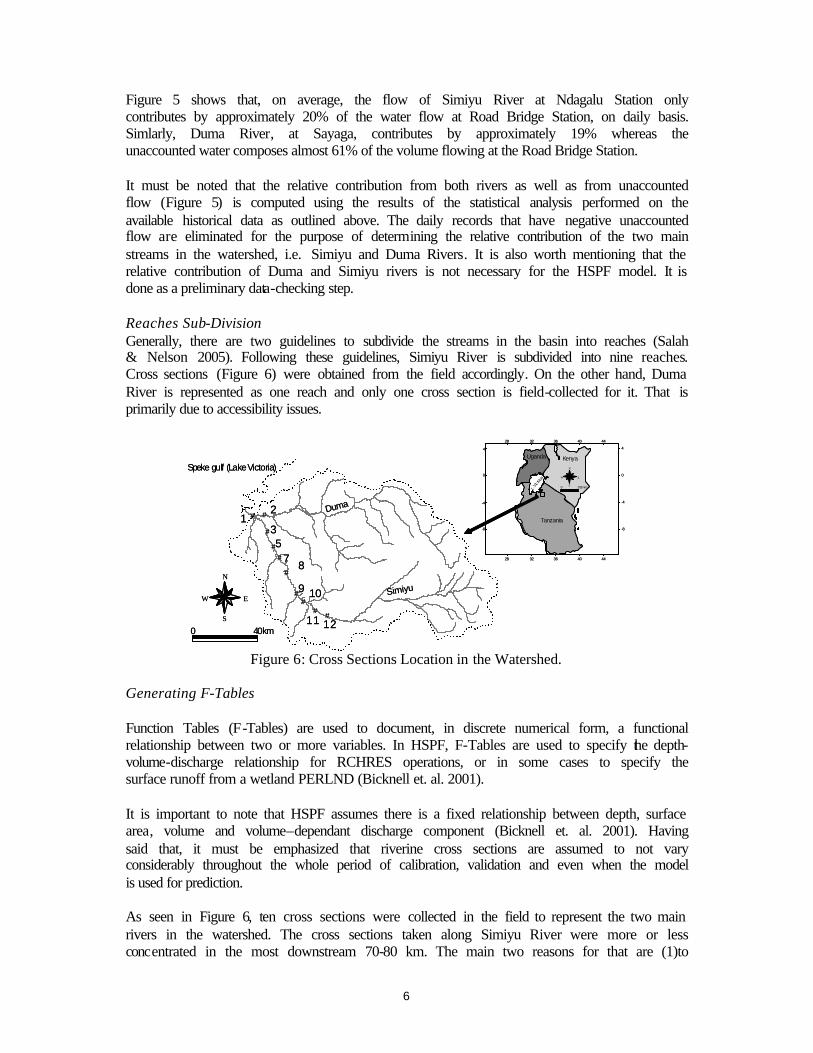
Figure 5 shows that, on average, the flow of Simiyu River at Ndagalu Station only contributes by approximately 20% of the water flow at Road Bridge Station, on daily basis. Simlarly, Duma River, at Sayaga, contributes by approximately 19% whereas the unaccounted water composes almost 61% of the volume flowing at the Road Bridge Station. It must be noted that the relative contribution from both rivers as well as from unaccounted flow (Figure 5) is computed using the results of the statistical analysis performed on the available historical data as outlined above. The daily records that have negative unaccounted flow are eliminated for the purpose of determining the relative contribution of the two main streams in the watershed, i.e. Simiyu and Duma Rivers. It is also worth mentioning that the relative contribution of Duma and Simiyu rivers is not necessary for the HSPF model. It is done as a preliminary data-checking step. Reaches Sub-Division Generally, there are two guidelines to subdivide the streams in the basin into reaches (Salah & Nelson 2005). Following these guidelines, Simiyu River is subdivided into nine reaches. Cross sections (Figure 6) were obtained from the field accordingly. On the other hand, Duma River is represented as one reach and only one cross section is field-collected for it. That is primarily due to accessibility issues.

N

EW

S0 200 km

Tanzania

KenyaUganda

L.Vic toria

28

28

32

32

36

36

40

40

44

44

-8 -8

-4 -4

0 0

4 4

##

#

#

##

#

##

#11

109

87

53

21

12

N

EW

S

0 40km

Speke gulf (LakeVictoria)

Duma

Simiyu

N

EW

S0 200 km

Tanzania

KenyaUganda

L.Vic toria

28

28

32

32

36

36

40

40

44

44

-8 -8

-4 -4

0 0

4 4

##

#

#

##

#

##

#11

109

87

53

21

12

N

EW

S

0 40km

Speke gulf (LakeVictoria)

Duma

Simiyu

Figure 6: Cross Sections Location in the Watershed.

Generating F-Tables Function Tables (F-Tables) are used to document, in discrete numerical form, a functional relationship between two or more variables. In HSPF, F-Tables are used to specify the depth-volume-discharge relationship for RCHRES operations, or in some cases to specify the surface runoff from a wetland PERLND (Bicknell et. al. 2001). It is important to note that HSPF assumes there is a fixed relationship between depth, surface area, volume and volume–dependant discharge component (Bicknell et. al. 2001). Having said that, it must be emphasized that riverine cross sections are assumed to not vary considerably throughout the whole period of calibration, validation and even when the model is used for prediction. As seen in Figure 6, ten cross sections were collected in the field to represent the two main rivers in the watershed. The cross sections taken along Simiyu River were more or less concentrated in the most downstream 70-80 km. The main two reasons for that are (1)to

7

account for the most geo-morphological changes in the river where flows reach significant values as opposed to upstream sections of the river and (2)the upper catchement has limited accessibility. WMS is used (Salah & Nelson 2005) to build the f-tables for HYDR section in the RCHRES application module in our model. Meteorological and Hydrological Time Series HSPF requires eight meteorological time series to simulate the hydrological cycle in a watershed. These are air temperature, dew point temperature, cloudiness, wind velocity, atmospheric pressure, solar radiation, potential evapotranspiration and precipitation (Albek et. al. 2004). Not all of them are available for our model in a complete form, or at least they do not span the same time frame. However, the model can still be built using the “best available” data. The time series used in our model are just two out of these eight; i.e. precipitation and pan evaporation covering the same period of time (1970-1978). Fine Tuning WMS interface is also used to define mass links and any external sources/targets as needed (Nelson 2004), (Salah & Nelson 2005). Mass links contain the specific time series to be transferred from one operation to another. They also contain the specific unit conversion factors that are needed. External sources specify time series, which are input to operations from external sources, WDM file for example. On the other hand, external targets specify time series, which are output from operations to external destinations. User Control Input File Finally, HSPF interface in WMS is used, as outlined above, to generate the User Control Input (UCI) file which is the main input to HSPF. The model runs and the output time series is added to the WDM file . The initial set of model parameter values is chosen based on experience, observations, previous research or other theoretical considerations (Nelson 2004), (Saleh & Du 2004). However, most of these initial values end up being changed in the calibration process, especially the process related parameters. Some fixed variables, do not change in the calibration process or at least are assumed to be fixed. Process related parameters are the main ones that are manipulated during calibration (Salah & Nelson 2005). Model Output WDMUtil (Hummel et. al. 2001) is a straightforward, easy-to-use tool that enables modelers to build or update WDM files. The goal of WDMUtil is to import/update available meteorological data and other time series into WDM files and to perform needed operations (e.g. editing, aggregation/disaggregation, filling missing data, etc.) to create input time-series for HSPF. The run adds another time series to the WDM file. In our case, WDMUtil is used to create the WDM file and to visualize both observed and simulated hydrographs. The initial “reconnaissance” run (Figure 7) demonstrated that there is a considerable difference between the simulated and observed flow data, hence there is a need for model calibration.

8

Figure 7: Initial "reconnaissance" Model Run; Discharges at Road Bridge.

Figure 7 shows the observed stream flow (solid blue line) and the simulated one (dashed red line). Visual comparison is not always enough for comparing two time series especially of this nature. Linear regression (Figure 8) analysis is performed to compare the two data sets. It is found that the intercept is 17.01 with a p-value (a measure of significance) of 0.000, and the slope is 0.08 with a p-value of 0.000. This shows that there is no evidence of a support to neglect the intercept and conclude that the slope is equal to 1.0 (i.e. observed is equal or close to the simulated values). This result supports the need for calibration and validation.

Observed

Sim

ulat

ed

Intercept

Slope

Simulated = Slope * Observed + interceptSimulated = Slope * Observed + intercept

Observed

Sim

ulat

ed

Intercept

Slope

Simulated = Slope * Observed + interceptSimulated = Slope * Observed + intercept

Figure 8: Linear Regression Analysis for Simulated vs Observed.

Calibration and Validation The only time period that has available discharge data overlapped in the three stations is between 1970 and 1978. The model is calibrated using flow data starting 1st January 1970 till 31st December 1975 from the gauging station at the Road Bridge (Station 112022) (Figure 9). Stream flows starting 1st January 1976 till 15th September 1978 at the same station are used to validate the model (Figure 10). HSPF is one of the data intensive models. It requires numerous parameters (e.g., over 100 parameters for the hydrologic process alone) to be inputted (Saleh & Du 2004). The first set of values (Table 1) used to run the initial model were adapted after recommended ranges (Bicknell et. al. 2001), (Salah & Nelson 2005) and (Saleh & Du, 2004). These values were then modified during the calibration process.

9

Table 1: List of Some Adjusted Parameters During Calibration. Recommended Range * Parameter Units

Min Max Calibrated value

AGWETP -- 0.000 1.000 0.000 AGWRC --/day 0.600 0.999 0.996 BASETP -- 0.000 1.000 0.001 CEPSC Mm 0.000 250.0 2.540

DEEPER -- 0.000 1.000 0.800 INFEXP -- 0.000 10.000 2.300 INFILT mm/hr 0.025 25 7.100

IRC --/day 1e-6 0.999 0.999 KVARY --/mm 0.000 2.000 0.000 LZETP -- 0.000 0.999 0.050

LZS Mm 0.025 2500 25 LZSN Mm 2.500 358 25.000

PETMAX oC -- -- 4.4 PLSNSUR -- 0.001 1.000 0.150

UZSN Mm 0.250 127 29.000 * After (Saleh & Du, 2004). Model calibration is an iterative procedure that can be simplified with the help of some tools. Such tools-aided calibration process is sometimes referred to as automatic calibration. However, in our case, the calibration iterations are manually done until a relatively satisfactory statistical result is obtained. The calibrated values listed in Table 1 represent the final values at the last iteration. Figure 9 shows the simulated and the observed stream flows for Simiyu watershed at Road Bridge Station. Similarly, Figure 10 shows observed and validated stream flows for Simiyu watershed at Road Bridge Station. The last calibration iteration is used to validate the model throughout the validation period.

Figure 9: Final, Calibrated Model Run.

10

Figure 10: Validating the Calibrated Model.

It is apparent in both Figure 9 and Figure 10 that the two hydrographs demonstrate an overall relative agreement, although the model tends to over-predict discharges especially in the winter. Simulated peak discharges are reasonably consistent with measured ones. Validation period tends to show more discrepancies than the calibration period. However, the overall simulated trend seems to be very well matching the observed one for both calibration and validations periods. Results and Discussion Even though visual inspection of Figure 9 and Figure 10 indicated a relatively good agreement between the observed and the simulated flows, statistical tests still need to be made to compare the observed daily stream flows to the simulated ones after calibration. A robust statistical test, of which its assumptions are not violated, needs to be incorporated at this stage. Since each simulation is relatively unique, there exists no single statistical test that can be valid universally across all cases of linear association. Each case should be examined individually to verify that assumptions of the used statistical test are not violated. The familiar Pearson’s correlation coefficient is not considered in our case, as the observed flow is not normally distributed (Figure 4b). Instead, the linear regression analysis examining the slope and intercept (Figure 8) is considered as a robust statistical test, in this case, to measure the linear association between the observed and simulated daily stream flows at the Road Bridge Station.. To test if the simulated and the observed flow values are in agreement, linear regression is used. We will refer to this as calibration assessment curve. Observed flow values (response variable) are regressed on the simulated values (explanatory variable). The main idea is to check if the slope of the explanatory variable is significant and close to unity and that the intercept is not significant (or significant and equal to zero). If this holds true, we could suggest that observed values are equal to the simulated ones (as it will form one single line on which any point will have the same values on both explanatory and response variables (Figure 8) ). The calibration assessment curve is done on both the calibration and the validation portions of the model ( Table 2 ).

11

Table 2: Calibration Assessment Curve for Calibration and Validation.

Intercept Slope Value 2.44 0.84

p-value (significance) 0.46 0.00 90% C.I. lower bound -3.25 0.72

Calibration

90% C.I. upper bound 8.13 0.96 Value 4.05 0.72

p-value (significance) 0.13 0.08 90% C.I. lower bound 2.4 0.62

Validation

90% C.I. upper bound 5.7 0.82 As shown in Table 2, the p-values for the intercept in both calibration and validation indicate that we fail to reject the null hypothesis (i.e. the intercept is equal to zero). Thus, there is no evidence that the intercept is significant. This is also supported by the 90% confidence interval that is containing zero for the calibration period. On the other hand, the relatively small p-values for the slope, for both calibration and validation, indicate that the null hypothesis can be rejected for the slope (i.e. the slope is , then, not equal to zero). Thus there is evidence that the slope is significant. Since, the value of the slope is ranging between 0.72 and 0.96 for calibration and between 0.62 and 0.82 for validation in a 90% confidence interval; we could say that the slope of the calibration assessment curve is considered to be close to 1.0 and accordingly the daily simulated flows can be considered equal to the observed ones during the calibration period. The calibration assessment curve assured, what was noticed in Figure 10, that the validation period does not show, at least relatively, the same agreement between observed and simulated discharges as in the calibration period. Before we reach concluding remarks for this paper, we must emphasize that the dead storage/ponds seem to have some effect on the hydrologic response of the basin. On the other hand, looking closely at the observed flow data set, and considering the ephemeral nature of the streams in the basin, is another indication of a need to model enhancements. Conclusion and Recommendations Using any model to simulate long term hydrological behavior of a given watershed is not an easy task. Most, if not all, model input parameters vary significantly with seasons and hydrological/meteorological conditions. The overall trend, peaks and valleys should be examined as opposed to localized differences. These localized differences will always exist in long term hydrological models and they should not disturb modelers as long as there is an overall acceptable agreement between the simulated and the observed flows. AS indicated in the results and discussion section, the statistical tests on the developed model indicate that there is no evidence of a considerable difference between the simulated and the observed daily stream flows. Hence, it can be generally used with confidence to predict future behavior of the watershed. However, it must be noted that the model is calibrated and validated on stream flow data during the period 1970 through 1978.

12

Detailed measurements/estimation of parameters AGWRC, DEEFR, KVARY, LZETP, LZSN and INFEXP might lead to better and easier calibration process for this watershed. This will definitely enhance any future modeling assignment as it will direct the attention of modelers towards the parameters that affect the model the most. It is recommended that the observed discharge data be further revised and verified. This conforms to the results of previous research efforts in the watershed. Moreover, there are time series that are not implemented to the model because of lack of data. Filling this gap will also enhance the model. Further research for Simiyu watershed should be focused on getting detailed cross sections on the Duma River. Also continuous monitoring of discharge data into both Simiyu and Duma Rivers is necessary for future refinement of the model. Moreover, the unaccounted flow at the watershed outlet is considerable. In that sense, it might be better to model the two sub-basins separately, as opposed to collectively model the whole basin. That is primarily because of the unidentified behavior of the basin. On the other hand, a better picture on the unaccounted flow will help in modeling the watershed as a whole, if needed. Future modifications to the model are required to improve predictions obtained. Re-calibrating/validating the model using more recent data will definitely enhance the simulative power of the model. Using automatic calibration tools, such as HSPEXP (Lumb et. al. 1994) and PEST (Papadopulos 2004), is another venue that will contribute to reducing calibration time/effort considerably. Acknowledgement This paper was prepared based on the research activities of the FRIEND/Nile Project which is funded by the Flemish Government of Belgium through the Flanders-UNESCO Science Trust Fund cooperation and executed by UNESCO Cairo Office. The authors would like to express their great appreciation to the Flemish Government of Belgium, the Flemish experts and universities for their financial and technical support to the project. The authors are indebted to UNESCO Cairo Office, the FRIEND/Nile Project management team, overall coordinator, thematic coordinators, themes researchers and the implementing institutes in the Nile countries for the successful execution and smooth implementation of the project. Thanks are also due to UNESCO Offices in Nairobi, Dar Es Salaam and Addis Ababa for their efforts to facilitate the implementation of the FRIEND/Nile activities.

13

Bibliography Cited Albek M, Ogutveren U.B., Albek E. (2004), “Hydrological Modeling of Seydi Suyu Watershed (Turkey) with HSPF”, Journal of Hydrology, Vol. 285, P.260-271, ELSEVIER. Bicknell B.R., Imhoff J.C., Kittle J.L., Jobes T.H., Donigian A.S. (2001), “Hydrological Simulation Program-Fortran (HSPF), version 12, User’s Manual”, AQUA TERRA Consultants, Mountain view, California, U.S.A. Cotter A.S., Chaubey I., Castello T.A., Soerens T.S., Nelson, M.A. (2003), “Water Quality Model Output Uncertainty as Affected by Spatial Resolution of Input data ”, Journal of the American Water Resources Association (JAWRA), Volume 39, Issue 4, 977-986. Hummel P., Kittle J., Gray M. (2001), “WDMUtil, version 2.0, User’s Manual”, AQUA TERRA Consultants, Decatur, Georgia, U.S.A., United States Environmental Protection Agency, 1200 Pennsylvania Ave, NW, Washington, DC, U.S.A. Johnson M.S., Coon W.F. Mehta V.K. Steenhuis T.S. Brooks E.S. Boll J. (2003), “Application of Two Hydrologic Models with Different Runoff Mechanisms to a Hillslope Dominated Watershed in Northeastern US: A comparison of HSPF and SMR”, Journal of Hydrology, Vol. 284, P.57-76, ELSEVIER. Lumb, A.M., McCammon, R.B., and Kittle, J.L., Jr., 1994, Users Manual for an expert system, (HSPEXP) for calibration of the Hydrologic Simulation Program – Fortran: U.S. Geological Survey Water-Resources Investigation Report 94-4168,102 p. Munson, A. D. (1998), “HSPF modeling of the Charles River Watershed ”, M.Sc. thesis Department of Civil Engineering, Massachusetts Institute of Technology. Nelson, E. J. (2004), “Watershed Modeling System, version 7.1, Tutorial”, Department of Civil and Environmental Engineering, Environmental Modeling Research Laboratory, Brigham Young University, Provo, Utah, U.S.A. Papadopulos S.S. & Associates, Inc. (2004), “PEST, Parameter Estimation” and “Calibrating a HSPF Model Using TSPROC and PEST”. Web site, URL: http://www.sspa.com/pest/pestsoft.html. Salah A., Nelson E.J. (2005), “Water Resources/Quality Modeling using Hydrological Simulation Program-Fortran (HSPF) and Watershed Modeling System (WMS); Technical Concerns Resolved”, International conference of UNESCO FLANDERS FIT FRIEND?NILE Project, Towards a better cooperation, 12-15 November 2005, Sharm El-Sheikh, Egypt, in press. Saleh A., Du B. (2004), “Evaluation of SWAT and HSPF within BASINS Program for the Upper North Bosque River Watershed in Central Texas”, Transactions of the ASAE, Vol. 47(4), P.1039-1049, American Society of Agricultural Engineers.

Long Term Hydrologic Modeling for Simiyu … Long Term Hydrologic Modeling for Simiyu Watershed,...

Documents

Transcript of Long Term Hydrologic Modeling for Simiyu … Long Term Hydrologic Modeling for Simiyu Watershed,...