
LONG TERM ACCRETION OF PHOSPHORUS IN WETLANDS: THE...
287
1 LONG TERM ACCRETION OF PHOSPHORUS IN WETLANDS: THE EVERGLADES STORMWATER TREATMENT AREAS AS A CASE EXAMPLE By RUPESH KUMAR BHOMIA A DISSERTATION PRESENTED TO THE GRADUATE SCHOOL OF THE UNIVERSITY OF FLORIDA IN PARTIAL FULFILLMENT OF THE REQUIREMENTS FOR THE DEGREE OF DOCTOR OF PHILOSOPHY UNIVERSITY OF FLORIDA 2013
Transcript of LONG TERM ACCRETION OF PHOSPHORUS IN WETLANDS: THE...

1
LONG TERM ACCRETION OF PHOSPHORUS IN WETLANDS: THE EVERGLADES STORMWATER TREATMENT AREAS AS A CASE EXAMPLE
By
RUPESH KUMAR BHOMIA
A DISSERTATION PRESENTED TO THE GRADUATE SCHOOL OF THE UNIVERSITY OF FLORIDA IN PARTIAL FULFILLMENT
OF THE REQUIREMENTS FOR THE DEGREE OF DOCTOR OF PHILOSOPHY
UNIVERSITY OF FLORIDA
2013

2
© 2013 Rupesh Kumar Bhomia

3
To my parents, Suresh and Santosh Bhomia

4
ACKNOWLEDGEMENTS
No words can describe my debt to my parents, who have encouraged and
motivated me throughout my life’s adventurous journey. This academic endeavor, one
of those adventures, would not have been successful without their profound love and
support. Equally important was my advisor – Dr. Reddy’s guidance and encouragement
that provided the necessary fuel for my progress. I am highly grateful for his patience
and persistent belief in my capabilities.
I am also thankful to the members of my supervisory committee - Dr. Mark
Brenner, Dr. Patrick Inglett and Dr. Alan Wright who guided me during my research
efforts. I thank Dr. Michael Chimney, external committee member, for fulfilling the role of
a critical reviewer and suggesting ideas that reinforced the importance of my work.
The importance of my research for meeting Everglades restoration goals was
recognized by two premier organizations themselves dedicated to the protection of the
Everglades ecosystem. I am thankful to both the South Florida Water Management
District and the Everglades Foundation for providing partial funding and technical
support for conducting my research. I would like to acknowledge specifically Ms. Delia
Ivanoff, Mr. Manuel Zamorano, Mr. Michael Korvela and Dr. Hongjun Chen from the
District, for extending technical help and field assistance for soil sample collection and
research.
I thank my swamp buddies – Michael Jerauld, Alex Cheesman and John Linhoss
who accompanied me during my multiple sorties to collect soil cores from the
Stormwater Treatment Areas in south Florida. I thank Michael Jerauld, Rohit Kanungo
and Christine VanZomeren for assistance in sample processing. Ms. Yu Wang and Mr.
Gavin Wilson methodically trained me on every laboratory procedure or equipment

5
operation that was carried out at the UF Wetland Biogeochemistry Laboratory. For initial
training and for elaborate discussions on lab instruments, analytical techniques and
generated data, I thank them greatly.
The staff at the Soil and Water Science Department – Mr. Michael Sisk, Ms.
Cheryl Combs, Ms. Linda Cowart, Ms. Lacey Givens and Ms. An Nguyen were
remarkable in taking care of all kinds of administrative tasks. I acknowledge their
eagerness to help and thank them fondly for their day-to-day assistance.
I recognize all the friendly folks – my fellow lab members and students for
indulging me into their world in many unique ways and for generously offering me the
benefits of their lively companionship. It is impossible to acknowledge all of them here,
but I warmly remember Mike Jerauld, Luke Gommerman, Justin Vogel, John Linhoss,
Casey Schmidt, Louis Philor, Pasicha Chaikaew, Dakshina Murthy, Daniel Irick, Jing
Hu, Christine VanZomeren, Rosalyn Johnson, Philip Alderman and Hugo Sindelar (RJ),
for interesting conversations and delightful discussions over cups of coffee or tasty
meals. Time spent in the company of these smiling faces was a truly rewarding
experience. I owe special thanks to Michael Jerauld and his parents for sharing a bond
of friendship that only grew stronger with time. I would like to thank Dr. Arun Jain, Ms.
Smita Jain and Ms. Janice Garry, friends outside of the UF network who had a positive
impact on me and were helpful in many ways.
I am highly indebted to Dr. Paromita Chakraborty for her true friendship and care
during the final stages of my dissertation research and writing. Finally, to my little
heroes – Milli and Joy (niece and nephew), whose sweet presence in my life makes
everything delightful and meaningful; I shall always remain grateful to them!

6
TABLE OF CONTENTS page
ACKNOWLEDGEMENTS ............................................................................................... 4
LIST OF TABLES ............................................................................................................ 9
LIST OF FIGURES ........................................................................................................ 13
ABSTRACT ................................................................................................................... 20
CHAPTER
1 INTRODUCTION .................................................................................................... 23
Treatment Wetlands................................................................................................ 24
Biogeochemical Processes .............................................................................. 26 Phosphorus Removal Mechanisms .................................................................. 29
Site Description ....................................................................................................... 33 Dissertation Overview ............................................................................................. 33
Dissertation Objectives and Hypotheses .......................................................... 34
Dissertation Layout ........................................................................................... 35
2 SPATIO-TEMPORAL CHANGES IN SOIL NUTRIENT STORAGE IN THE EVERGLADES STORMWATER TREATMENT AREAS: IMPACT ON PHOSPHORUS REMOVAL PERFORMANCE ....................................................... 41
Background ............................................................................................................. 41 Objectives and Hypotheses .................................................................................... 45 Methods .................................................................................................................. 46
Site Description ................................................................................................ 46 Data Sources .................................................................................................... 47
Soil Nutrient Mass Storages ............................................................................. 48 Phosphorus Mass Balance ............................................................................... 48 Data Analysis ................................................................................................... 50
Results .................................................................................................................... 51 Physico-Chemical Properties ........................................................................... 51 Phosphorus ...................................................................................................... 51
Nitrogen ............................................................................................................ 52
Carbon.............................................................................................................. 53 Mass Balance ................................................................................................... 53
Discussion .............................................................................................................. 54 Phosphorus Retention ...................................................................................... 55 Phosphorus Mass Balance ............................................................................... 57
Impact of STA Age on Phosphorus Retention .................................................. 58 Summary ................................................................................................................ 60

7
3 CHANGE POINT TECHNIQUE FOR MEASUREMENT OF SOIL ACCRETION RATES IN CONSTRUCTED WETLANDS .............................................................. 78
Background ............................................................................................................. 78
Methods .................................................................................................................. 80 Site Description ................................................................................................ 80 Soil Sampling and Processing .......................................................................... 82 Chemical and Isotopic Analysis ........................................................................ 82 Change-point Analysis ..................................................................................... 83
Results .................................................................................................................... 85 Discussion .............................................................................................................. 86
4 SOIL AND NUTRIENT ACCRETION RATES IN TREATMENT WETLANDS OF THE EVERGLADES BASIN ............................................................................ 100
Background ........................................................................................................... 100 Objectives and Hypotheses .................................................................................. 103
Methods ................................................................................................................ 104 Site Description .............................................................................................. 104
Soil Sampling and Processing ........................................................................ 105 Data Analysis ................................................................................................. 106 Mass Balances ............................................................................................... 107
Results .................................................................................................................. 108 Soil and Phosphorus Accretion Rates ............................................................ 109
Phosphorus Mass Balance ............................................................................. 110
Discussion ............................................................................................................ 110
Soil Physico-Chemical Properties .................................................................. 111 Soil and Phosphorus Accretion Rates ............................................................ 112 Phosphorus Mass Balance ............................................................................. 114
Summary .............................................................................................................. 115
5 STABILITY OF PHOSPHORUS IN RECENTLY ACCRETED SOILS: ASSOCIATED VEGETATION EFFECTS ............................................................. 127
Background ........................................................................................................... 127 Objectives and Hypotheses .................................................................................. 129
Methods ................................................................................................................ 129
Site Description .............................................................................................. 129 Soil and Chemical Analysis ............................................................................ 130 Soil Phosphorus Fractionation ........................................................................ 131
Data Analysis ................................................................................................. 132 Results .................................................................................................................. 133
Total Nitrogen ................................................................................................. 134 Total Carbon ................................................................................................... 134 Metals ............................................................................................................. 134 Phosphorus Fractions .................................................................................... 135 Vegetation Effects .......................................................................................... 136

8
Correlations Among Soil Properties ............................................................... 137 Discussion ............................................................................................................ 138 Summary .............................................................................................................. 141
6 CONCLUSIONS ................................................................................................... 164
Objective 1: Spatio-Temporal Changes in Soil Nutrient Storages ......................... 167 Objective 2: Soil Accretion in Treatment Wetlands ............................................... 168 Objective 3: Soil Accretion and Operational Age of Treatment Wetlands ............. 168 Objective 4: Stability of Phosphorus in Recently Accreted Soil ............................. 169
Synthesis .............................................................................................................. 170 Future Outlook and Sustainability of STAs ........................................................... 172
APPENDiX
A ADDITIONAL DATA AND INFORMATION PERTAINING TO CHAPTER 1 ......... 177
B ADDITIONAL DATA AND INFORMATION PERTAINING TO CHAPTER 2 ......... 179
C ADDITIONAL DATA AND INFORMATION PERTAINING TO CHAPTER 3 ......... 186
D ADDITIONAL DATA AND INFORMATION PERTAINING TO CHAPTER 4 ......... 191
E ADDITIONAL DATA AND INFORMATION PERTAINING TO CHAPTER 5 ......... 248
LIST OF REFERENCES ............................................................................................. 266
BIOGRAPHICAL SKETCH .......................................................................................... 287

9
LIST OF TABLES
Table page 2-1 Bulk density for floc and soil samples from the STAs. ........................................ 62
2-2 Mean floc depth across the STAs for sampling years. ........................................ 63
2-3 Total phosphorus concentration in floc and soils in the STAs. ........................... 63
2-4 Total phosphorus areal storage in floc and soils in the STAs ............................. 64
2-5 Comparison of total phosphorus removed from the water column and floc phosphorus storage and soil phosphorus storage. ............................................. 64
2-6 Total nitrogen areal storage in floc and soils in the STAs ................................... 65
2-7 Total carbon areal storage in floc and soils in the STAs ..................................... 66
2-8 Variation in areal and total nutrient storages in the STAs with different ages. Nutrient masses represent entire floc depth and top 10 cm of surface soil.. ...... 66
3-1 Soil accretion measurement methods and published accretion rates from wetland studies. .................................................................................................. 91
4-1 Soil and phosphorus accretion rates in STA-1W, STA-2 and STA-3/4 ............. 117
5-1 Summary statistics for bulk density of soil sections in EAV and SAV cells of STA-1W and STA-2 .. ....................................................................................... 142
5-2 Summary statistics for loss on ignition of soil sections in EAV and SAV cells of STA-1W and STA-2 ...................................................................................... 142
5-3 Summary statistics for total phosphorus content of soil sections in EAV and SAV cells of STA-1W and STA-2 .. ................................................................... 143
5-4 Summary statistics for total phosphorus storage pools for each soil fraction in EAV and SAV cells of STA-1W and STA-2....................................................... 143
5-5 Summary statistics for total nitrogen content of soil sections in EAV and SAV cells of STA-1W and STA-2. ............................................................................. 144
5-6 Summary statistics for total nitrogen storage pools for each soil fraction in EAV and SAV cells of STA-1W and STA-2....................................................... 144
5-7 Summary statistics for total carbon content of soil sections in EAV and SAV cells of STA-1W and STA-2 .............................................................................. 145

10
5-8 Summary statistics for total carbon storage pools for each soil fraction in EAV and SAV cells of STA-1W and STA-2. .............................................................. 145
5-9 Summary statistics for calcium content of soil sections in EAV and SAV cells of STA-1W and STA-2. ..................................................................................... 146
5-10 Summary statistics for magnesium content of soil sections in EAV and SAV cells of STA-1W and STA-2. .............................................................................. ............................................ 146
5-11 Summary statistics for iron content of soil sections in EAV and SAV cells of STA-1W and STA-2 . ........................................................................................ 147
5-12 Summary statistics for aluminum content of soil sections in EAV and SAV cells of STA-1W and STA-2 .. ........................................................................... 147
5-13 Summary statistics for phosphorus content in P fractions in floc, RAS and pre-STA soil from EAV and SAV cells in STA-1W and STA-2 .......................... 148
5-14 Summary statistics for phosphorus content in P fractions in floc, RAS and pre-STA soil from EAV and SAV cells in STA-1W ............................................ 149
5-15 Summary statistics for phosphorus content in P fractions in floc, RAS and pre-STA soil for EAV and SAV cells in STA-2 .................................................. 149
5-16 Pearson correlation coefficients for select parameters measured in all soil fractions in both STA-1W and STA-2 .. ............................................................. 150
5-17 Pearson correlation coefficients for select parameters measured in all soil fractions in EAV cells from both STA-1W and STA-2 ....................................... 151
5-18 Pearson correlation coefficients for select parameters measured in all soil fractions in SAV cells from both STA-1W and STA-2. ...................................... 152
5-19 Pearson correlation coefficients for select parameters measured in all soil fractions from STA-1W . ................................................................................... 153
5-20 Pearson correlation coefficients for select parameters measured in soil fractions from STA-2. ........................................................................................ 154
A-1 Treatment Wetland Technology conferences ................................................... 177
B-1 Mean total nitrogen concentration in floc and soils in STAs. ............................ 182
B-2 Mean total carbon concentration in floc and soils in STAs ............................... 183
B-3 STA performance for WY2011 and the period of record. .................................. 184

11
C-1 Number of 2-cm sections produced by sectioning soil cores collected from STA-1W. ........................................................................................................... 186
C-2 Number of 2-cm sections produced by sectioning soil cores collected from STA-2. .............................................................................................................. 186
C-3 Number of 2-cm sections produced by sectioning soil cores collected from STA-3/4. ........................................................................................................... 187
D-1 STA-1W soil core collection sites by vegetation type and cell. ......................... 194
D-2 STA-2 soil core collection sites by vegetation type and cell. ............................ 194
D-3 STA-3/4 soil core collection sites by vegetation type and cell........................... 195
D-4 Summary statistics for change point depths calculated with SegReg in soil cores collected from STA-1W, STA-2 and STA-3/4. ......................................... 196
D-5 Bulk density profiles in soil cores collected from each cell of STA-1W ............. 197
D-6 Total phosphorus profiles in soil cores collected from each cell of STA-1W ..... 198
D-7 Bulk density and total phosphorus profiles in soil cores collected from each cell of STA-2. .................................................................................................... 199
D-8 Bulk density and total phosphorus profiles in soil cores collected from each cell of STA-3/4 .................................................................................................. 200
E-1 STA-1W and STA-2 soil core collection sites by vegetation type and cell ........ 248
E-2 Mean depth of RAS at STA-1W sampling sites used for separating RAS from pre-STA soil. ..................................................................................................... 249
E-3 Mean depth of RAS at STA-2 sampling sites used for separating RAS from pre-STA soil.. .................................................................................................... 249
E-4 Depth of soil fraction, bulk density, total phosphorus concentration and TP storage for each soil fraction at sampling sites in STA-1W. .............................. 250
E-5 Depth of soil fraction, bulk density, total phosphorus concentration and TP storage for each soil fraction at sampling sites in STA-2. ................................. 251
E-6 Depth of soil fraction, bulk density, total nitrogen concentration and TN storage for each soil fraction at sampling sites in STA-1W. .............................. 253
E-7 Depth of soil fraction, bulk density, total nitrogen concentration and TN storage for each soil fraction at sampling sites in STA-2. ................................. 254

12
E-8 Depth of soil fraction. bulk density, total carbon concentration and TC storage for each soil fraction at sampling sites in STA-1W. ........................................... 256
E-9 Depth of soil fraction, bulk density, total carbon concentration and TC storage for each soil fraction at sampling sites in STA-2. .............................................. 257
E-10 Average total phosphorus concentration and TP storage for each soil fraction over all sampling sites in EAV and SAV cells of STA-1W ................................. 259
E-11 Average total phosphorus concentration and TP storage for each soil fraction over all sampling sites in EAV and SAV cells of STA-2 .................................... 259
E-12 Average total nitrogen concentration and TN storage for each soil fraction over all sampling sites in EAV and SAV cells of STA-1W ................................. 260
E-13 Total nitrogen concentration and TN storage for each soil fraction over all sampling sites in EAV and SAV cells of STA-2. ................................................ 260
E-14 Total carbon concentration and TC storage for each soil fraction over all sampling sites in EAV and SAV cells of STA-1W. ............................................ 261
E-15 Total carbon concentration TC and storage for each soil fraction over all sampling sites in EAV and SAV cells of STA-2. ............................................... 261
E-16 Pearson correlation coefficients for select parameters measured in soil cores from EAV cells of STA-1W ............................................................................... 262
E-17 Pearson correlation coefficients for select parameters measured in soil cores from SAV cells of STA-1W ............................................................................... 262
E-18 Pearson correlation coefficients for select parameters measured in soil cores from EAV cells of STA-2. .................................................................................. 263
E-19 Pearson correlation coefficients for select parameters measured in soil cores from SAV cells of STA-2 ................................................................................... 263

13
LIST OF FIGURES
Figure page 1-1 Cross section view of emergent and submerged aquatic vegetation in free
water surface wetlands.. ..................................................................................... 37
1-2 Common biogeochemical processes with regard to phosphorus cycling in typical free water surface wetland ...................................................................... 38
1-3 Map showing the locations of the original six Stormwater Treatment Areas, the Everglades Agricultural Area and the Everglades Protection Area in South Florida. ..................................................................................................... 39
1-4 Configuration of the treatment cells within each Stormwater Treatment Area .... 40
2-1 Phosphorus mass balance calculations for soil P storage with respect to net P retained from the water column. ...................................................................... 67
2-2 Relationship between STA age and fraction of total phosphorus storage in floc and soil derived from the water column ....................................................... 68
2-3 Relationship between total P retained from the water column through WY2007 and total P storage in floc and soil ....................................................... 69
2-4 Relationship between total P retained from the water column and total P storage in floc and soil... ..................................................................................... 70
2-5 Relationship between total P retained from water column and total P storage in floc and soil.. ................................................................................................... 71
2-6 Relationship between floc total P concentration and inflow total P flow-weighted mean concentration. ............................................................................ 72
2-7 Relationship between floc P storage and inflow total P flow-weighted mean concentration. ..................................................................................................... 73
2-8 Relationship between soil carbon storage and soil P storage in WY2007. ......... 74
2-9 Phosphorus mass balance calculations for soil P storage with respect to net P retained from the water column.. ..................................................................... 75
2-10 Relationship between mean floc P storage per year and STA age.. ... ............... 76
2-11 Relationship between mean surface soil P storage per year and STA age.. ...... 77
3-1 Location of the STA-1W, STA-2 and STA-3/4 and the number of soil cores collected from each STA. ................................................................................... 94

14
3-2 A cross-section view of a typical free water surface treatment wetland and schematic depiction of a boundary between recently accreted soil and pre-STA soil .............................................................................................................. 95
3-3 SegReg output using bulk density, total phosphorus content, and stable isotopic ratios of C and N in a representative soil profile from STA-2. ................ 96
3-4 Depth of RAS for STA-1W, STA-2, and STA-3/4 as determined by SegReg change-points using bulk density, total phosphorus, isotope ratio of C and N... ...................................................................................................................... 97
3-5 Variation in RAS depth between two dominant vegetation types – Emergent Aquatic Vegetation and submerged aquatic vegetation for four parameters - bulk density, total phosphorus, stable isotope ratio of C and N.. ........................ 98
3-6 Comparison of RAS depth obtained by using SegReg program and 137Cs peaks from Everglades Water Conservation Area-2.. ......................................... 99
4-1 Location of the STA-1W, STA-2 and STA-3/4 and the number of soil cores collected from each STA. ................................................................................. 118
4-2 Phosphorus mass balance calculations for soil P storage with respect to net P retained from the water column.. ................................................................... 119
4-3 Differences in soil profile bulk density and total phosphorus content between two vegetation communities, in STA-1W, STA-2 and STA-3/4. .... ................... 120
4-4 Differences in soil profile δ15N (‰) and δ13C (‰) between two vegetation communities, EAV and SAV, in STA-1W, STA-2 and STA-3/4. .. ..................... 121
4-5 Differences in soil profile C:N ratio and N:P ratio between two vegetation communities, EAV and SAV, in STA-1W, STA-2 and STA-3/4. ........................ 122
4-6 RAS depth as determined using change-point analyses for different cells of STA-1W, STA-2, STA-3/4 and for entire STA. .. ............................................... 123
4-7 Soil accretion rate as a function of STA age for STA-1W, STA-2 and STA-3/4. ................................................................................................................... 124
4-8 Phosphorus accretion rate as a function of STA age for STA-1W, STA-2 and STA-3/4.. .......................................................................................................... 125
4-9 Phosphorus mass balance calculations for soil P storage with respect to net P retained from the water column . ................................................................... 126
5-1 Location of soil sampling sites in the STAs. Field triplicate sites are shown ..... 155
5-2 Phosphorus fractionation scheme used to characterize P forms in STA soils. . 156

15
5-3 Phosphorus content and relative proportion of P fractions (organic, inorganic and residual P) in floc, RAS and pre-STA soil of STA-1W. ............................... 157
5-4 Phosphorus content and relative proportion of P fractions (organic, inorganic and residual P) in floc, RAS and pre-STA soil of STA-2.. ................................. 158
5-5 Inorganic P content plotted against TP for all soil sections in EAV and SAV cells from STA-1W and STA-2. ......................................................................... 159
5-6 Organic P content plotted against TP in EAV and SAV cells from STA-1W and STA-2 ........................................................................................................ 159
5-7 Percent composition of stable and reactive phosphorus pools in the floc, RAS and pre-STA soil of EAV and SAV cells for STA-1W and STA-2 ...................... 160
5-8 Non-reactive phosphorus as a fraction of total phosphorus in floc, RAS and pre-STA soil of STA-1W and STA-2. ................................................................ 161
5-9 Relationship between phosphorus and calcium in EAV and SAV cells of STA-1W. . ................................................................................................................. 162
5-10 Relationship between phosphorus and calcium in EAV and SAV cells of STA-2. ...................................................................................................................... 163
6-1 Summary of total phosphorus loading rates, TP accretion rates and distribution of reactive and non-reactive TP pools of STA-2. ............................ 176
C-1 Soil core sampling locations in each cell of STA-1W ........................................ 188
C-2 Soil core sampling locations in each cell of STA-2 ........................................... 189
C-3 Soil core sampling locations in each cell of STA-3/4.. ...................................... 190
D-1 Soil depth profiles from STA-1W. ..................................................................... 201
D-2 Soil depth profiles from from STA-2. ................................................................. 202
D-3 Soil depth profiles from STA-3/4. ...................................................................... 203
D-4 Bulk density profile in each soil core collected from STA-1W. .......................... 204
D-5 Total phosphorus profile in each soil core collected from STA-1W ................... 211
D-6 Bulk density profile in each soil core collected from STA-2. ............................. 218
D-7 Total phosphorus profile in each soil core collected from STA-2.. .................... 223
D-8 Bulk density profile in each soil core collected from STA-3/4.. ......................... 228

16
D-9 Total phosphorus profile in each soil core collected from STA-3/4. .................. 238
E-1 Relation of TP with Po and Pi and LOI with Po in floc, RAS and pre-STA soil from EAV and SAV cells of STA-1W.. .............................................................. 264
E-2 Relation of TP with Po and Pi and LOI with Po in floc, RAS and pre-STA soil from EAV and SAV cells of STA-2. ................................................................... 265

17
LIST OF ABBREVIATIONS
ADW Agricultural Drainage Water
AFDW Ash Free Dry Weight
Al Aluminum
BD Bulk Density
BMP Best Management Practices
C Carbon
Ca Calcium
CAB Cellulose Acetyl Butyrate
CPT Change-point Technique
EAA Everglades Agricultural Area
EAV Emergent Aquatic Vegetation
ECP Everglades Construction Project
ENRP Everglades Nutrient Removal Project
EPA Everglades Protection Area
FAV Floating Aquatic Vegetation
Fe Iron
FEFA Florida Everglades Forever Act
FL Florida
FCS Floc Carbon Storage
FNS Floc Nitrogen Storage
FPS Floc Phosphorus Storage
FWMC Flow-Weighted Mean Concentrations
FWS Free Water Surface
HCl Hydrochloric Acid

18
HSSF Horizontal Subsurface Flow
LOI Loss on Ignition
Mg Magnesium
N Nitrogen
NaOH Sodium Hydroxide
NMR Neutron Magnetic Resonance
NPDES National Pollution Discharge Elimination System
NPP Net Primary Productivity
P Phosphorus
PS Phosphorus Storage
PAR Phosphorus Accretion Rate
POR Period of Record
RAS Recently Accreted Soils
REE Rare Earth Elements
RPM Revolution per Minute
SAR Soil Accretion Rate
SAV Submerged Aquatic Vegetation
SD Standard Deviation
SET Sediment Elevation Table
SFER South Florida Environment Report
SFWMD South Florida Water Management District
SCS Soil Carbon Storage
SNS Soil Nitrogen Storage
SPS Soil Phosphorus Storage
SRP Soluble Reactive Phosphorus

19
STA Stormwater Treatment Area
TC Total Carbon
TN Total Nitrogen
TP Total Phosphorus
USACE United States Army Corps of Engineers
USEPA United States Environmental Protection Agency
VF Vertical Flow
WCA Water Conservation Areas
XANES X-ray Absorption Near Edge Structure

20
Abstract of Dissertation Presented to the Graduate School of the University of Florida in Partial Fulfillment of the Requirements for the Degree of Doctor of Philosophy
LONG TERM ACCRETION OF PHOSPHORUS IN WETLANDS: THE
EVERGLADES STORMWATER TREATMENT AREAS AS A CASE EXAMPLE
By
Rupesh Kumar Bhomia
May 2013
Chair: K. Ramesh Reddy Major: Soil and Water Science
The presence of excess nutrients in an environment can negatively affect the
ecological integrity of natural systems and lead to loss of ecosystem functions. Aquatic
ecosystems experience impairment of natural structure and functions due to high
nutrient inputs. Constructed treatment wetlands are often utilized to transform, modify or
store excess nutrients and protect downstream ecosystems. This study was conducted
to enhance our understanding of select biogeochemical processes that control
treatment performance, efficiency and long-term sustainability of such constructed
wetlands. Large constructed wetlands in south Florida, the Everglades Stormwater
Treatment Areas (STAs), were selected as the experimental sites for this research.
These STAs were built to treat surface runoff originating in the Everglades Agricultural
Area (EAA) by removing excess phosphorus (P) from the water before it flows into the
Everglades.
The overarching goal of this dissertation research was to understand key
processes that control and regulate transformation of P from the reactive (potentially
bio-available) fraction into the non-reactive (stable) fractions. Associated pathways for
this transformation were also investigated to determine treatment wetlands (STAs)

21
capability to provide long-term sustainable storage of the sequestered P. This task was
carried out by analyzing long-term soil P data obtained from various STAs and
conducting experiments to quantify and characterize soil P storage pools and functional
chemical P forms within the STAs that have been in operation for 10-16 years.
Spatio-temporal variation in floc, recently accreted soil (RAS) and pre-STA
(antecedent) soil P storage pools was calculated by utilizing existing information from
soils monitoring. Stratigraphic properties of soil profiles were utilized to determine the
boundary between RAS and pre-STA soil, which were then used to calculate accretion
rates in the STAs. An inverse relationship was found between accretion rates and
operational age of the STAs, suggesting that the rate of new soil formation decreased
over time. Using soil P pools, and P retained from the water column, P mass balances
for the STAs were developed. Phosphorus mass balance calculations indicated that a
large portion of P in RAS sections was probably mined from deeper soil sections.
The quality and quantity of sequestered P has profound implications for the
interaction and fate of P in the STAs, hence chemical characterization of accreted P
was done by using operationally defined P fractionation schemes. Effects of STA age
and dominant vegetation on chemical partitioning of accreted P were investigated.
Fractionation analysis showed that about 70% of P in the RAS section was in reactive
form, i.e., potentially vulnerable to mobilization. The relative proportion of reactive and
non-reactive P pools within emergent and submerged aquatic vegetation cells were
similar across the studied STAs. Greater proportions of reactive P pools were observed
in floc and RAS sections of SAV cells in comparison to EAV cells. In other words, floc
and RAS sections of SAV cells contain larger proportion of reactive P than in floc and

22
RAS of EAV cells. Strong positive correlation between TP and calcium (Ca) in floc and
RAS layers suggested Ca-P co-precipitation as the dominant mechanism of P removal
in SAV cells. Among reactive P pools, the Pi pool was higher in SAV cells while Po pool
was greater in EAV cells.
Long-term effectiveness and sustainability of treatment wetlands is important to
meet treatment targets and protect downstream targets. This dissertation research was
designed to advance our understanding of the extent and quality of P pools in treatment
wetlands to allow for better planning and management under conditions of
environmental uncertainty.

23
CHAPTER 1 INTRODUCTION
Wetlands are dynamic ecosystems characterized by unique hydrology, soils,
vegetation and high net primary productivity (NPP) (Keefe, 1972; Westlake, 1963). As a
transitional ecotones between terrestrial and aquatic ecosystems, wetlands fulfill a vital
role in the landscape continuum (Sheaves, 2009). These productive ecosystems are a
source of many direct and indirect benefits (Blackwell and Pilgrim, 2011; Costanza and
others, 1997) and more recently wetlands have been a major catalyst in transforming
modern society’s perspective on the value of ecosystem services offered by other
natural ecosystems (Maltby and Acreman, 2011).
As natural systems, wetlands are increasingly considered valuable capital
assets1 (Barbier, 2011; Daily and others, 2000) that provide important services including
water quality improvement (Gilliam, 1994; Kadlec and others, 1979; Moshiri, 1993; Van
der Valk and Jolly, 1992; Verhoeven and others, 2006), flood abatement (Potter, 1994),
ground water discharge-recharge (Acharya, 2000), biodiversity enhancement (Erwin,
1990; Mitsch and others, 2009), and a variety of recreational (Bergstrom and others,
1990) and educational opportunities (Sukhontapatipak and Srikosamatara, 2012).
These services are a net outcome of several biophysical processes that take place
within a wetland. These complex processes are often bundled together in a single term,
‘wetland functions’, which is used frequently in discussions pertaining to valuation of
nature (De Groot, 1992). The ability of natural wetlands to improve water quality is one
such function that depends on existing biogeochemical and physical conditions uniquely
present in a wetland environment. Recognition of a wetland’s potential to treat polluted
1 Asset can be defined as an economic resource that can produce a flow of beneficial goods and services
over time.

24
waters resulted in efforts to create artificial wetlands for abating unwanted contaminants
in water. Early research in this direction began in 1952 when Dr. Käthe Seidel, Max
Planck Institute, started experimenting with macrophytes to treat wastewater (Bastian
and Hammer, 1993). Currently thousands of functioning constructed wetlands are
located globally across multiple geographic regions in both developed and developing
nations.
Treatment Wetlands
Constructed wetlands are used for reduction of nutrient loads in surface runoff to
protect downstream ecosystems. Impacts from excess nutrient availability are known to
degrade the natural balance of aquatic ecosystems (Belanger and others, 1989; Smith,
2003; Verhoeven and others, 2006), hence constructed wetlands are specifically
designed and strategically positioned on the landscape to transform and assimilate
excess nutrients by utilizing natural biogeochemical processes (Brix, 1993; Solano and
others, 2004; USEPA, 2000; Vymazal, 2005). Given their ability to ‘treat’ water,
constructed wetlands specifically created for water quality enhancement purposes are
referred to as ‘treatment wetlands’.
Constructed treatment wetlands are usually managed to function as buffers to
retain or transform excess nutrients and harmful contaminants (Kadlec and Wallace,
2009; Shutes, 2001). Surface waters that do not meet water quality standards because
of point or nonpoint sources of pollution can be treated by these wetlands (Babatunde
and others, 2008; Day and others, 2004). In the past two decades, treatment wetlands
have gained considerable popularity as an effective, low-cost alternative to conventional
wastewater treatment approaches (Table A-1, Appendix A). Treatment wetlands are
mechanically simple, require low energy inputs, and generally have low operational and

25
management costs except where cost of land is high since treatment wetlands are often
land intensive (Iovanna and others, 2008). Additionally, treatment wetlands can be
designed across a broad realm of operational scales ranging in size from smaller units
capable of treating wastewaters from only a few households to large systems covering
many hectares and treating high volumes of agricultural or stormwater runoff (Chen,
2011).
Treatment wetlands often are designed based on outflow nutrient (pollutant)
target concentrations and operating condition (local climatic conditions). Various
configurations are available to meet desired performance goals , efficiency, biotic
community and preferred level of intervention (Brix, 1993). Three major categories of
treatment wetlands based on hydraulic flow are:
Free-water surface (FWS) wetlands: Water flows on the surface and contains areas of open water, just like natural marshes. These wetlands support emergent aquatic vegetation (EAV) and submerged or floating aquatic vegetation (SAV or FAV; Figure 1-1).
Horizontal subsurface flow (HSSF) wetlands: Water flows horizontally within the substrate from the inlet to the outlet. The substrate is usually coarse gravel planted with wetland vegetation.
Vertical Flow (VF) wetlands: Water flow is predominantly vertical from the substrate to the overlying water column, and the site of treatment is mostly the plant root zone.
This dissertation research is focused on FWS treatment wetlands, which are
widely popular because of their resilience to adverse climatic factors, and ability to cope
with pulse flows and changing water levels (Kadlec and Wallace, 2009). FWS wetlands
resemble natural marshes, with submerged and emergent vegetation communities
interspersed with patches of open water. These wetlands are commonly used to treat

26
urban, agricultural and industrial runoff; however, their use in treating mine waters,
leachate and polluted ground water has also been successfully demonstrated.
Biogeochemical Processes
Water quality improvement by treatment wetlands is achieved by modification,
transformation and storage of excess nutrients and pollutants (Kadlec and Wallace,
2009; Shutes, 2001). The main processes that remove contaminants from water include
sedimentation, mechanical filtration, oxidation, reduction, adsorption, absorption,
precipitation, microbial immobilization, transformation and vegetative uptake. This is
possible primarily as a consequence of air-soil-water-vegetation ‘interfaces’ where the
vegetation and microbial communities interact and participate in various biogeochemical
processes (Reddy and DeLaune, 2008). The relative rates of these coupled
biogeochemical processes vary across time and space, with incidences of intermittent
fast reactions -‘hot moments’2 and the presence of active action sites -‘hot spots’
(McClain and others, 2003). Wetlands are therefore well suited to transform influent
chemicals into products that could be internally assimilated or exported from the
system. Gaseous products (N2, CH4, CO2, H2S, NH3, and N2O) are often lost to the
atmosphere whereas dissolved forms (NH4+, PO4
-, NO3-, etc.) are immobilized by the
microbial or vegetative communities (Reddy and DeLaune, 2008; Vymazal, 2007).
Particulate forms can be exported from the system as a result of high hydraulic flows, or
can remain trapped in low flow conditions. The physical settling of suspended organic
and inorganic particulates and deposition of plant litter result in the formation of new
2 Biogeochemical hot spots are patches that exhibit disproportionately high reaction rates relative to the
surrounding matrix, whereas hot moments are defined as short periods of time that exhibit disproportionately high reaction rates relative to longer intervening periods.
27
material at the soil-water interface (DeBusk and Reddy, 1998). This newly accumulated
organic layer is composed of both allochthonous and autocthonous material and may
represent various stages in the ‘decay continuum’ as labile constituents are slowly lost
while recalcitrant fractions accumulate over time (Melillo and others, 1989). The
residence time of recalcitrant constituents in accreted soils is often high, and due to this
long-term storage capability, wetlands are often characterized as nutrient sinks (Nichols,
1983; Reddy and Gale, 1994).
At the elemental level, carbon (C) is the primary driver of all the biogeochemical
processes in wetlands (Prairie and Cole, 2009; Reddy and DeLaune, 2008) and
phosphorus (P), nitrogen (N), and sulphur (S) cycling is tightly coupled with organic
matter turnover in wetlands (Reddy and others, 1999a; Wetzel, 1992). Numerous
studies have been conducted to understand the scope, scale and associated pathways
for macro-elemental processing in natural and treatment wetlands. Some noteworthy
examples include - carbon (Alvarez-Cobelas and others, 2012; Battin and others, 2009;
Boon and Mitchell, 1995), nitrogen (Bachand and Horne, 2000; Lund and others, 2000;
Spieles and Mitsch, 2000), phosphorus (Fennessy and others, 2008; Lund and others,
2001; Nairn and Mitsch, 2000; Pant and others, 2002; Reddy and others, 1999b; Wang
and Mitsch, 2000) and sulphur (Mandernack and others, 2000; Morgan and
Mandernack, 1996; Rudd and others, 1986; Spratt and Morgan, 1990). These studies
have advanced our knowledge to refine design criteria for meeting performance targets
in treatment wetlands. Although more than a thousand treatment wetlands are currently
operational throughout the world (Kadlec and Wallace, 2009), active research efforts to
optimize performance have been undertaken only on a small proportion of them (Reddy

28
and others, 2006). This dissertation presents one such effort aimed towards a detailed
understanding of the complex processes controlling pollutant removal mechanisms in
treatment wetlands. By studying selective wetlands constructed for trapping excess P
from runoff originating on farms in the Everglades Agricultural Area (EAA), an attempt is
made to understand key regulators of treatment performance over time, and assess the
long-term sustainability outlook of those treatment wetlands.
The Everglades, historically an oligotrophic ecosystem, experienced an
unprecedented input of P as a byproduct of agricultural and urban development during
the mid-twentieth century (Richardson, 2010). The impacts due to excessive P influx
has been widely documented for the greater Everglades ecosystem (Noe and others,
2001; Reddy and others, 2011). These impacts include reduced productivity of
submerged plants and benthic periphyton, depletion of dissolved oxygen in the water,
and changes in invertebrate and vertebrate community structure (Crozier and Gawlik,
2002; Smith and others, 2009). The most conspicuous change in the Everglades has
been the expansion of monotypic stands of cattail (Typha spp.) that displaced the
indigenous sawgrass community (Cladium jamaicense Crantz) (Daoust and Childers,
2004; Sklar and others, 2005; Vaithiyanathan and Richardson, 1999).
Phosphorus is included in fertilizers and feed supplements to meet the
requirement of agricultural crops and livestock and enable continued higher yields,
however unutilized P is susceptible to loss from the agricultural fields or livestock feed
lots. Because P in all its various forms is non-volatile, it follows hydrologic pathways and
often gets concentrated in wetlands and inland water bodies after being introduced in
the environment (Reddy and others, 1999a). In the past two decades much effort has

29
gone into restoring the Everglades to its original hydrologic flow and ecological condition
(Chimney and Goforth, 2006). As a potential remedy, thousands of hectares of artificial
treatment wetlands, Stormwater Treatment Areas (STAs), were created to remove
excess P from surface runoff before this water reaches the Everglades. STAs are
actively managed to maintain optimum operational status and meet performance goals
mandated by the Everglades Forever Act (EFA). The National Pollutant Discharge
Elimination System (NPDES) provides regulatory framework under which STA’s
operating permits are administered.
Phosphorus Removal Mechanisms
In wetland soils, P predominantly forms complexes within organic matter in peat
lands (Cheesman and others, 2010; Fisher and Reddy, 2010) or inorganic sediments in
mineral-soil wetlands (Walbridge, 1991). Phosphorus occurs as soluble or insoluble
organic or inorganic complexes. The relative proportion of each form depends on soil,
vegetation and land-use characteristics of the drainage basin. The particulate and
soluble organic fractions can be further separated into labile and refractory components.
Physico-chemical transformations convert organic and particulate P into biologically
available inorganic forms which is utilized by micro-organisms and vegetation. The
bioavailable P fraction triggers growth responses in flora and fauna and can cause a
shift from oligotrophic to eutrophic state when P concentrations are sufficiently high. It is
essential that the STAs operate to maximize production and storage of refractory
components while minimizing loss of bioavailable P fractions to meet Everglades
restoration goals.
The relative rates of coupled biogeochemical processes in the STAs regulate
long-term accretion of P. In general, two classes of processes, biotic and abiotic,

30
mediate these transformations (Withers and Jarvie, 2008). Biotic processes include
assimilation by vegetation, plankton, periphyton and microorganisms. Abiotic processes
include sedimentation, adsorption by soils, precipitation, and exchange processes
between sediment and the overlying water column. These abiotic and biotic processes
are detailed in Figure 1-2 with a cross-section view of a typical FWS wetland. The STAs
are representative examples of FWS wetlands.
In general, four main processes contribute to P retention in the STAs - sorption to
soil solids, sedimentation, co-precipitation and biological uptake. Movements of P onto
and off of sites on the surface of soil solids are called adsorption and desorption,
respectively. Adsorption/desorption equilibria are reached shortly after there is a change
occur in pore water P concentration (e.g., in response to external P inputs) (Froelich,
1988). Solid-state diffusion of adsorbed phosphate from the surface into the interior of
particles occurs over a longer duration (Froelich, 1988). The soil-water interface controls
nutrient concentrations (Li and others, 1972; Patrick and Khalid, 1974) in overlying
waters (net flux on or off the soil particles) as governed by the equilibrium phosphorus
concentration (EPCo) (Carritt and Goodgal, 1954). In wetlands, the amount of P that
can be adsorbed to the soils is often related to the soil iron (Fe) and aluminum (Al)
content (Lijklema, 1976). However, in the alkaline soils of south Florida, soil calcium
(Ca) also is an important determinant of soil P sorption capacity (Reddy and others,
1998). With regards to treatment wetlands’ potential for continued P removal, soil
adsorption is not considered a sustainable P removal mechanism because of relatively
fast reaction time and the finite sorption capacity of soils for P (Kadlec, 2009; Kadlec
and Wallace, 2009).

31
The suspended solids influx (load) to STAs includes eroded soil particles,
macrophyte detritus, and algae or other planktonic organisms, all of which contain P
(Stuck and others, 2001). The suspended forms settle out due to gravity under reduce
flow velocities or by being trapped within the litter layer or adhering to the biofilms
(Schmid and others, 2005). Sedimentation of suspended solids can account for a
significant portion of total P removal by STAs, and sustainability is constrained by
increase in bottom elevation due to sediment accretion that eventually will prevent
surface water flows.
Precipitation of P with Ca, Fe, Al and Mg cations represents an additional
pathway of P removal in wetlands (Reddy and others, 1999b; Reddy and others, 2005).
It is not easy to differentiate precipitation from adsorption because precipitates often
form on the surfaces of soil particles (Scinto and Reddy, 2003); hence this mechanism
is referred to as co-precipitation. Reddy and DeLaune (2008) provide a thorough
discussion on the conditions that promote P co-precipitation with available cations and
explain the processes that result in the formation of apatite (Ca5(Cl)(PO4)3) and
hydroxylapatite (Ca5(OH)(PO4)3) within Everglades soils (Reddy and D’Angelo, 1994;
Reddy and others, 1993). The actual mechanism underlying Ca-P association may be
either adsorption of P onto the surface of CaCO3 precipitates or the formation of mixed
crystals during co-precipitation (Otsuki and Wetzel, 1972; Scinto, 1997).
High primary productivity and associated P requirements make biological uptake
an important mechanism contributing to wetland P removal. Plants and microorganisms
typically utilize only dissolved Pi. Prior studies have investigated P uptake potential of
wetland plants (Greenway, 2003; Reddy and Debusk, 1985; Tanner, 1996) and algae

32
and other microorganisms (Havens and others, 1999). Nearly all of the P incorporated
into microbial biomass and majority of the macrophyte-P is returned to the P cycle
through decomposition (Kadlec and Wallace, 2009; Reddy and others, 1995). However,
reducing conditions in wetlands slow decomposition and, over time, results in organic
matter accumulation. The P fraction that is stored in refractory biomass compounds in
accrued sediments contributes to long-term sustainable P removal. The conditions
supporting and enhancing each of the above mentioned, four P removal mechanisms
depend on soil characteristics, vegetation type and abundance and water-column
chemistry, including cation availability and the distribution of the total P pool among the
various functional P forms. Maximizing P treatment in STAs requires an understanding
and quantification (and manipulation) of the relative contributions of each of these
processes to net P removal.
Performance of the STAs in terms of P removal is assessed by monitoring inflow
and outflow water quality parameters on a short time-scale (weekly or bi-weekly). In
addition, periodic soil and vegetation monitoring is conducted. The lack of detailed
information on P cycling among the active storage compartments (including water
column, plant biomass, surface litter and soil) is responsible for the ‘black box’ approach
still used to evaluate the Everglades STAs (Zurayk and others, 1997). In-depth
knowledge of key biogeochemical processes that regulate continued accrual of organic
matter, and promote transformation of reactive P forms into non-reactive forms is
necessary for designing interventions that will help STA to maintain optimum treatment
efficiency and meet mandated performance goals in future. Consolidation and
sophisticated integration of available information is required to derive critical

33
understanding that may be useful for long-term sustainability of the STAs. By using the
STAs as a case example, this dissertation examined the role of wetland vegetation, age
and soil nutrient storage in regulating P treatment efficiency. This study also explored
the relative stability of sequestered P in an attempt to determine long-term sustainability
of treatment wetlands, specifically in response to disturbances e.g. extreme weather
events or changes in the immediate environment such as pH and redox shifts.
Site Description
The study was conducted in the Everglades STAs, which are located south of
Lake Okeechobee in the state of Florida. The current network of six STAs occupies
approximately 18,000 hectares of land area and provides an economically feasible
means of reducing P inputs to the Everglades Protection Area (EPA) (Figure 1-3 and
Figure 1-4). A detailed description of the STA’s operational history and performance is
presented in Appendix B. The STAs are operated and managed by the South Florida
Water Management District (SFWMD). This dissertation presents results of studies
conducted in STA-1W, STA-2 and STA-3/4.
Dissertation Overview
The quality and quantity of sequestered P has immediate and profound
implications for STA treatment performance. A complex set of bio-geochemical
processes controls and regulates P cycling and dictates long-term stability of stored P.
Transformation of P from reactive pools to non-reactive pools within the STAs can be
considered a predictor of the long-term sustainability of STAs. The ultimate goal of this
dissertation was to investigate the fate of sequestered P in relation to the treatment
efficiency of the STAs over time.

34
This study began with the examination of spatio-temporal changes in P storages
in STA soils and then progressed to develop a novel technique for measuring soil
accretion rates in STAs. Relationship between soil accretion rates and operational age
of STAs was explored to determine impacts in P removal efficiency with time.
Phosphorus mass-balances were developed by quantifying P pools in recently accreted
soil (RAS) and antecedent pre-STA soil to determine allocation of P transferred from the
water column to various P storage compartments. Floc and RAS were characterized to
identify the relative proportions of various functional P forms to assess treatment
efficiency of the STAs. Finally, this information was synthesized to provide insights into
STA performance over the entire period of operation and assess the long-term
sustainability outlook for the STAs in the future.
Dissertation Objectives and Hypotheses
The first objective of this dissertation was to review available datasets on STA
soil physico-chemical variables and determine spatio-temporal changes in surface and
sub-surface soil nutrient storage to explore relationship between hydraulic and water
quality parameters, soil nutrient storages and STA age. These data were further used to
perform preliminary P mass balance. The hypothesis for this objective was that STAs’
treatment efficiency or P removal efficiency declines after a protracted period of
operation (Chapter 2). Objective 2 was to determine the soil accretion rate in the STAs,
by utilizing stratigraphic characteristics of the soil profiles to identify the boundary
between recently accreted soil (RAS) and antecedent pre-STA soil. The hypothesis
behind this objective was that the STAs are accreting systems and accumulating
organic matter conserves attributes of prevailing conditions (e.g. nutrient loading,
vegetation community). Changes in these stratigraphic characteristics can be exploited

35
to identify the depth of RAS deposited on top of pre-STA soil (Chapter 3). Objective 3
was to explore the relationship between soil accretion rates and operational age of the
STAs and perform P mass balance using P storages in RAS and pre-STA soil and the
amount of P removed from the water column. Cycling of P within different P storage
compartments of the STAs was also estimated. The main hypothesis for this objective
was that most of the P retained from the water column is stored in RAS, which has a
higher P concentration than pre-STA soil. With increasing age, the rate of soil and P
accretion declines, resulting in higher outflow P concentrations. Internal re-distribution of
P within RAS and pre-STA soil is mediated by vegetation. This controls whether the
STAs function as a nutrient source or sink (Chapter 4). Determination of the relative
proportion of reactive and non-reactive P pools in the STAs and assessment of the
influence of wetlands vegetation communities (EAV vs. SAV) on reactivity of P pools
was the fourth objective, addressed in (Chapter 5). I expected that differences in the
wetland vegetation types (EAV vs. SAV) will influence the proportion of P forms
incorporated into RAS and sequestered in the STAs. The presence of more reactive
(i.e., potentially mobile) P forms will reduce the long-term sustainability of the STAs.
Dissertation Layout
The dissertation is organized in 6 chapters. Chapter 1 (this chapter) introduces
the main processes occurring in the treatment wetlands, factors critical in controlling
long-term treatment efficiency and provides an overview of the objectives and rationale
behind the dissertation. This is followed by Chapter 2, which presents an analysis of
datasets on STA soil physico-chemical variables and spatio-temporal changes in
surface and sub-surface soil nutrient storages. After exploring the relationships between
hydraulic and water quality variables, soil nutrient storage and STA age, a preliminary P

36
mass-balance for STAs was conducted. Chapter 3 presents detailed information about
a novel change-point technique (CPT) that was developed to measure soil accretion
rates in wetlands. The CPT was used to determine the depth of recently accreted soil
(RAS) in select STAs. Chapter 4 focuses on the soil and P accretion rates that were
determined using RAS depths and operational age of the STAs. The relationship
between accretion rates and STA age is also presented. Influence of wetland vegetation
on accretion rates and P mass balance using RAS depth is also presented to show P
cycling through various P storage compartments in the STAs. Chapter 5 contains
results from the study on chemical characterization of functional P forms in RAS. This
was performed to determine the relative proportion of reactive and non-reactive P
storage pools. The role of vegetation and other geochemical variables were explored
and long-term sustainability of STAs was examined. Finally, Chapter 6 provides a
synthesis of conclusions drawn from all the dissertation studies.

37
Figure 1-1. Cross section view of emergent and submerged aquatic vegetation in FWS wetlands. Higher water depth
enables growth of submerged and floating aquatic vegetation.

38
Figure 1-2. Common biogeochemical processes with regard to phosphorus cycling in typical free water surface (FWS)
wetland. Arrows show direction of movement; size does not necessarily represent relative mass or volume of processes.

39
Figure 1-3. Map showing the locations of the original six Stormwater Treatment Areas
(STAs; in green), the Everglades Agricultural Area and the Everglades Protection Area in South Florida. Compartments B and C are expansions to the STAs and are indicated in red (Germain and Pietro, 2011).

40
Figure 1-4. Configuration of the treatment cells within each Stormwater Treatment Area (STA). The dominant vegetation type in each cell is also indicated (Germain and Pietro, 2011)

41
CHAPTER 2 SPATIO-TEMPORAL CHANGES IN SOIL NUTRIENT STORAGE IN THE
EVERGLADES STORMWATER TREATMENT AREAS: IMPACT ON PHOSPHORUS REMOVAL PERFORMANCE
Background
Constructed wetlands exhibit a broad range of biogeochemical and physical
characteristics, and are utilized worldwide for enhancing aspects of surface water
quality (Brix, 1994; Kadlec and Wallace, 2009). These artificial ecosystems are
designed to reduce the concentration of water-borne contaminants by either
transforming or assimilating pollutants. Constructed treatment wetlands are particularly
popular for intercepting agricultural drainage waters (ADW), which often contain high
concentrations of nutrients such as nitrogen (N) and phosphorus (P). Such is the case
with large-scale treatment wetlands in south Florida, which were constructed as filtration
marshes to remove excess nutrients from surface runoff before it enter the Everglades
(Figure 1) (Chimney and Goforth, 2001; Goforth, 2001; Perry, 2004; Redfield, 2000).
These wetlands are referred to as the Everglades STAs, and are tasked with reducing
total P (TP) concentrations in surface runoff to ecologically benign levels (Walker,
1995). The strategic location of the STAs has allowed them to retain over 1,450 metric
tons of P, which has resulted in a considerable load reduction of P to the Everglades.
STA outflow total P flow-weighted mean concentrations (FWMC) were reduced from
152 µg P L-1 to 38 µg P L-1 during the period from 1994 to 2011 (Ivanoff and others,
2012).
High P loads in an oligotrophic system are known to cause a shift in the
ecosystem’s biotic communities by disrupting natural nutrient characteristics and can
ultimately lead to eutrophic or hyper-eutrophic conditions (Khan and Ansari, 2005).

42
Following excessive P inputs, the northern Everglades ecosystem has exhibited signs of
widespread impaired ecosystem function, including extensive growth of Typha spp.
(cattail) in place of the natural inhabitant, Cladium jamaicense (sawgrass) (Hagerthey
and others, 2008; Vaithiyanathan and Richardson, 1999).
To counter these undesirable changes, the Comprehensive Everglades
Restoration Plan (CERP) was developed with a goal to restore, protect and preserve
the remaining Everglades ecosystem (USACE and SFWMD, 2000). The CERP is
broadly aimed at improving quality, quantity, timing and flow of water for both ecological
integrity and human needs in south Florida. A major component of this plan, water
quality improvement, includes reduction of P inputs by implementing best management
practices (BMPs) in the EAA (Diaz and others, 2005; Izuno and Capone, 1995; Rice
and others, 2002) and subsequent treatment of ADW that leaves the EAA. Treatment is
carried out by intercepting ADW in the STAs where biogeochemical processes remove
P from the water column (DeBusk and others, 2001a; Gu and others, 2001; Nungesser
and Chimney, 2001).
The first full-scale treatment wetland in south Florida, known as the Everglades
Nutrient Removal Project (ENRP), became operational in 1994 (Chimney and others,
2006; Guardo and others, 1995). Subsequent expansion of the ENRP and addition of
new STAs led to the current STAs’ total footprint of approximately 18,000 ha of effective
treatment area (Ivanoff and others, 2012). Although the STAs have sequestered a
substantial amount of P during their operational history, they are known to exhibit
variable treatment performance in terms of P removal efficiency over time (Pietro and
others, 2008). The spatio-temporal variability in STA treatment performance has been

43
attributed to factors such as antecedent land use, vegetation condition and species
composition, nutrient and hydraulic loading, hydraulic residence time, hydroperiod, soil
characteristics and P content, cell topography and configuration, extreme weather
events, construction activities and regional operations (Germain and Pietro, 2011). A
study conducted on 49 treatment wetlands found that TP removal was more a function
of mean hydraulic residence time than mean hydraulic loading rate (Carleton and
others, 2001). However, a broader overview of P removal performance across a range
of FWS wetlands suggested that background concentrations, P loading rates (PLR),
temperature and seasonal effects and ecological variables such as water depth and
vegetation type and cover, etc. are the main controlling factors (for details see Chapter
10, Kadlec and Wallace, (2009)). This review also recognized constraints in P
processing when low outflow concentrations are required, which highlights the
challenges experienced by the Everglades STAs where outflow TP FWMCs are
currently mandated to be in the 13-19 µg P L-1 range.
A thorough examination of 21 variables including inflow TP concentration,
hydraulic and TP loading rates, TP fractions, calcium (Ca) and pH did not yeild a single
variable that has greatest influence in controlling TP concentration or TP areal settling
rate in STAs (Jerauld, 2010). This study, however, emphasized the importance of
background soil P concentration and also showed an inverse relationship between STA
ages and outflow TP concentrations (Jerauld, 2010). STA age could be a key factor in
determining STA performance because it is a lumped term that represents multiple
wetland characteristics that change over time, such as soil P and plant biomass and
tissue P concentrations. Further information on key factors affecting performance of

44
treatment wetlands in general, and the STAs in particular, are presented in Chapter 1 as
a review of published literature (Carleton and others, 2001; Carleton and others, 2000;
Carleton and Montas, 2010; Chimney and Pietro, 2006; Dierberg and others, 2002a;
Dierberg and others, 2005; Fisher and Reddy, 2010; Gu and others, 2001; Gu, 2006;
Gu, 2008; Ivanoff and others, 2012; Juston and DeBusk, 2006; Juston and DeBusk,
2011; Kadlec, 1997; Kadlec, 1999; Kadlec, 2005; Kadlec and Hammer, 1988; Kadlec
and Wallace, 2009; Luderitz and Gerlach, 2002; Martin and Anderson, 2007;
McCormick and Odell, 1996; Moustafa and others, 1996; Nouri and others, 2010;
Nungesser and Chimney, 2001; Pietro and others, 2006; Reddy and others, 1999a;
Richardson, 1985; Richardson and Qian, 1999; Walker and Kadlec, 2011).
Juston and DeBusk, (2006) explored relationships between mass loading of P
and subsequent outflow concentrations within the STAs and compared them with seven
other treatment wetlands in Florida. Their analysis of historic data concluded that a
long-term average annual PLR at or below ∼1.3 g m-2 yr-1 is conducive to outflow TP
concentrations less than ~ 30 µg P L-1 irrespective of vegetation type (Juston and
DeBusk, 2006). An extensive study of the Everglades STAs for the entire period of
operation (1994- 2011) found a significant positive correlation between PLR and outflow
TP concentration, with dramatic increases in outflow concentrations from STAs when
PLR was greater than ∼1.0 g m-2 yr-1 (Ivanoff and others, 2012). This analysis also
elucidated differences in vegetative response to PLR, with a substantially greater
increase in outflow TP concentration in EAV cells in comparison to SAV cells at PLRs
greater than ∼1.0 g m-2 yr-1(Ivanoff and others, 2012). However, EAV cells are typically

45
situated in the front end of STA flow-ways, which experience higher inflow TP
concentrations, which may affect outflow TP concentrations.
Performance of the STAs for regulatory compliance is quantified by measuring
hydrologic parameters, i.e. volume and chemical characteristics of inflow and outflow
waters to and from STAs. This approach overlooks the complex biogeochemical
processes that regulate P removal from the water column and controls the stability of
sequestered P pools in the STAs. With continued STA operation, P removed from the
water column accumulates as recently accreted organic soil and contributes to the
incremental enrichment of the surficial layer of soil, potentially leading to the saturation
of internal P storage compartments (Lowe and Keenan, 1997). Recently accreted soils
(RAS) share an active interface with floc (unconsolidated detritus that is deposited on
the consolidated wetland surface layer) and the overlying water column, and depending
on the existing biogeochemical factors, nutrient concentrations in the RAS layer could
potentially influence STA TP outflows (White and others, 2006). Therefore, an
understanding of the complex processes that regulate long-term sustainable P removal
in the STAs is desired for effective management and for meeting Everglades restoration
goals. An assessment and characterization of nutrient storages in STA soils could be
the first step towards dismantling the black-box-like approach (Zurayk and others, 1997)
used to evaluate treatment wetland function. Investigation of changes in soil P storages
over temporal and spatial scales could provide meaningful insights into STA
performance and P removal efficiency over time.
Objectives and Hypotheses
The main objective of this study was to review available datasets on STA soil
physico-chemical parameters and determine spatio-temporal changes in surface and

46
sub-surface soil nutrient storages. Subsequently, relationships between hydraulic and
water quality parameters, soil nutrient storage and STA age were investigated to
explore the trajectory of TP removal efficiency in aging STAs. A preliminary TP mass
balance was performed to understand where the bulk of retained P was distributed
within the STA soil profile. These objectives were supported by the hypothesis that TP
removal efficiency of STA declines after a continued period of operation. In addition,
internal redistribution of P within soil profiles, mediated by vegetation, controls overall P
removal efficiency of STAs.
Methods
A comprehensive review of existing information on STA soil nutrient storage was
conducted to document changes in soil nutrient status over time and to explore
relationships between soil P storage and TP retained from the water column. Surface
soil P storages in all six STAs were compared to explore the effect of STA age on TP
removal rates. Phosphorus distribution within various compartments of STAs – water
column, floc, surface soils (0-10 cm), and sub-surface soils (below 10 cm) was
determined. Temporal changes in P storage within these compartments was used to
generate estimates of P flux, which was then used to develop overall TP mass balances
for the STAs.
Site Description
The Everglades STAs have a combined surface area of approximately 26,300
ha, with about 18,000 ha of effective treatment area (Ivanoff and others, 2012). This
area is distributed among six STAs, each of which is comprised of multiple,
independently managed units called cells (Figure 1-4). Each cell is actively managed to
have one dominant vegetation community depending on the intended treatment

47
objectives. The two broad categories of vegetation are emergent aquatic vegetation
(EAV) and submerged aquatic vegetation (SAV) [SAV cells also contain floating aquatic
vegetation (FAV) species]. The South Florida Water Management District (SFWMD) is
responsible for operating, maintaining and optimizing the performance of all the STAs to
ensure compliance with operating permits. The six operational STAs include: STA-1E
and STA-1W, STA-2, STA-3/4, STA-5, and STA-6. A detailed description of STAs and
associated TP removal is presented in Table B-3 (Appendix B).
Data Sources
Data used in this study were obtained from the SFWMD and the Wetland
Biogeochemistry Lab (WBL), University of Florida. Detailed information regarding
operations and management of STAs was obtained from South Florida Environment
Reports (SFERs) (Chimney and others, 2000; Germain and Pietro, 2011; Ivanoff and
others, 2012; Pietro and others, 2010). Data used for this analysis represented 495 floc
samples and 1700 soil samples spanning the entire period of record (POR) for all STAs
up to water year (WY) 2008 [Each WY runs from May 1 through April 30 of the following
calendar year].
Sampling dates indicated that STA soils were collected approximately every
three years from WY2004 through WY2008; however, the earliest data from WY1994
was obtained from STA-1W. Floc depth was variable across sample sites. Soil cores
were divided into two sections – surface soils (0-10 cm) and sub-surface soil (10-30
cm).
Floc and soil dataset used for analysis contained physico-chemical information
such as bulk density, ash free dry weight (AFDW), organic matter content (loss on
ignition; LOI), pH, iron (Fe), Ca, sulfur (S), total carbon (TC), TP and total nitrogen (TN).

48
Using bulk-density, core depth and soil nutrient concentrations, P, C and N storage
within floc, surface soils and sub-surface soils was determined. Nutrient storage was not
calculated where floc depth, bulk density or nutrient concentration data was missing.
Soil Nutrient Mass Storages
Total nutrients (C, N and P) storage in floc (variable depth) and soils (0-10 and
10-30 cm) were calculated. Mean floc depth for each sampling event was used for
calculating P, N and C storage in the floc fraction while a depth of 10 cm was universally
used for surface soil storage calculations. Nutrient storage per unit area (g m-2) for both
floc and soil layers was calculated as follows:
FXS = (CX* Dfb * df)/100 ………………. (2-1)
SXS = (CX * Dsb * ds)/100 ..……………... (2-2)
where,
FXS = Floc nutrient (X) storage (g m-2)
SXS = Soil nutrient storage (g m-2)
X = Nutrient X (carbon, nitrogen or phosphorus)
Cχ = Nutrient concentration (mg kg-1)
Dfb = Bulk density of floc (g m-3)
Dsb = Bulk density of soil (g m-3)
df = Depth of floc (cm)
ds= Depth of soil (cm)
Relationships between TP retained by the STAs and P mass storage (g P m-2) in
floc and the top 10-cm surface soils were explored. The effect of STAs age on floc and
soil P mass storage was examined for all STAs. Relationships between TP areal
storage in the STAs and concomitant C and N mass storage was also explored.
Phosphorus Mass Balance
Mass balances can be calculated with varying degrees of complexity, either
considering only the mass of P that entered but did not leave a wetland (by subtraction
of outflow from inflow data) (Boyt and others, 1977; Sloey and others, 1978) or, through

49
quantification of P flux, across various compartments within the wetland (soil and
biomass) and finally P storage in soils (Dolan and others, 1981; Fetter and others, 1978;
Headley and others, 2003; Lee and others, 2012). Even simple P mass balances are
useful in determining the sources of P to the wetland (surface water, groundwater,
precipitation) and for calculating gross P removal effectiveness (Bhadha and others,
2011; Chung and others, 2008). More complex ‘complete’ mass balances are
increasingly difficult to assemble owing to sample collection and processing challenges
(Correll, 1998), but may aid in illuminating internal processes that could be useful to the
understand fate of retained nutrients by the STAs. Phosphorus mass-balances
performed as a part of this study utilized an approach with somewhat greater level of
complexity involving cumulative TP retained from the water column (P Wc; g P m-2) by
STAs over their POR (up through WY2008) and corresponding changes in areal P mass
storage (g P m-2) in floc and the top 10-cm of surface soil (Figure 2-1).
The difference between floc P storage (FPS; g P m-2) and P Wc indicated net
movement of P within floc and surface soil layer and was represented as Pflux F. The
sign of Pflux F, ‘-ve’ or ‘+ve’, indicated direction of P enrichment (movement), with +ve
Pflux F signifying flux from the underlying surface soil layer into the floc layer. Conversely,
FPS smaller than P Wc indicated net movement of P down into the surface soil (Pflux F; -
ve), this would be the case when floc gets consolidated and transformed into soil.
The earliest available soil P storage (SPS; g P m-2) for the top 10-cm of surface
soil was used as background P (PBG) and was subtracted from WY2007 SPS. A net
positive change indicated P enrichment of the surface horizon either from the floc above
(Pflux F; -ve) or from the subsurface soil below (Pflux SS; +ve; Figure 2-1). Soil P storage in

50
WY1995 was used as the background (PBG) for STA-1W while SPS in WY2005 was
taken as background for both STA-1E and STA-3/4. Soil PS in WY2001 was used as
background for STA-2, STA-5 and STA-6. The arrows in Fig. 2-1 indicate the direction
of P flux (g P m-2) from one storage compartment to another.
For all practical purposes, soils represent the only long-term nutrient storage pool
in wetlands while nutrients in live vegetation serve only as a temporary transient pool
(Howard-Williams, 1985), hence P present in vegetation was not considered for TP
mass-balance calculations. Critical assumptions made for developing TP mass
balances for the STAs are listed below:
The total mass of TP retained from the water column (P Wc) initially resides as floc, therefore floc P storage (FPS) at any given time reflects the fraction of TP incorporated from the water column as well as contribution from vegetative detrital matter (physical settlement of particulate forms, adsorption-absorption of soluble forms, biological immobilization by microbial communities).
Floc P contributed by vegetative detrital matter deposition may represent a fraction that could be obtained from underlying soils by rooted plants (EAV) or directly from the water column by submerged and floating plants (SAV/FAV). For comparisons at STA level, both EAV and SAV/FAV cells within one STA were averaged to obtain FPS for that STA.
Floc becomes soil over time, so with a long observation period some of the water-column TP have passed through the floc and into the surface soil.
Flux of P from underlying soil (Pflux SS) to overlying soil or floc is regulated by redox conditions and the equilibrium P concentration (EPCo).
Phosphorus in live vegetation biomass at a given time (i.e., plant standing stock) accounts for only a tiny fraction of TP in the STAs and represents a transient pool which ultimately gets transformed into floc and soil after plant senescence, following the decay continuum pathway.
Data Analysis
All calculations and comparison of nutrient storage pools were performed using
Excel. Nutrient mass storages were not calculated if floc depth, bulk density

51
measurements or nutrient concentrations were unavailable. Total P storage in analyses
represented floc and 0-10 cm soil P storages. Area-weighted mean values were used to
determine nutrient storages within each STA cell, which were then added together to
provide total storage for the whole STA in a given year. Relationships within nutrient
mass storages in STA soils, and between STA age and soil and floc P storages were
explored using Excel spreadsheet regression models.
Results
Physico-Chemical Properties
Among all STAs, floc and soil bulk density were highest in STA-1E, suggesting
these is much higher mineral fraction in the surface soils (Table 2-1). Floc bulk density
ranged from 0.04 to 0.26 g cm-3 whereas soil bulk density varied from 0.2 to 1.0 g cm-3
across all STAs for all sampling events. The range of mean floc depth (cm) across
STAs was higher in WY2004 than in WY2007 (Table 2-2). Floc depth decreased in
STA-1W and STA-5, whereas it increased in STA-2 during this period.
Phosphorus
Floc and soil P concentrations (mg P kg-1) showed an increase from WY2004 to
WY2007 (Table 2-3). Floc P concentration was lowest in STA-2, whereas it was highest
in STA-1W. The range of soil P concentration was lowest in STA-1E and highest in
STA-5. Floc and soil P storage in STAs is presented in Table 2-4. In WY2007, STA-5
surface soils (0-10 cm) had highest P storage.
Caution should be exercised in comparing SPS in the 0-10 cm depth surface soil
across STAs. In older STAs, such as STA-1W, most of the 0-10 cm soil represents
consolidated floc and only some antecedent pre-STA soil. However, in younger STAs,
much of the 0-10 cm soil depth may represent pre-STA soil with only a small fraction

52
derived from consolidation of floc. Therefore comparing P storage in the top 10-cm of
surface soil across different STAs will represent dissimilar contributions from floc and
pre-STA soil depending on the operational age of STA, and the rate of soil accretion.
The percentage of TP (floc + soil) derived from water column as a function of STA’s
operational history is plotted in Figure 2-2. As the STAs aged, the percentage of TP
storage derived from water column increased (r2=0.86). However, no clear relationship
(r2=0.20) was observed between the mass of TP removed from the water column and
TP storage in WY2007 (Figure 2-3). The one to one line in Figure 2-3 differentiates
between the proportion of TP in floc + soil derived from pre-STA soil and TP transferred
from the water column. This indicated increasing proportion of TP in surface soils
because of net P retention from overlying water column with increasing STA’s age. A
comparison of TP retained from the water column during the operational history of STAs
and the amount stored in floc and soil is presented in Table 2-5.
There was no relationship when P storage was regressed against TP retained
from the water column for all STAs each water year (Figure 2-4). Similarly, no
relationship was obtained when cell averages were analyzed instead of whole STAs
(Figure 2-5). Additionally, when floc P concentrations (Figure 2-6) and floc P storages
(Figure 2-7) were regressed against inflow TP flow-weighted mean concentrations (μg P
L-1), no relationship was observed at the cell level.
Nitrogen
Total N concentrations (mg N kg-1) across STAs are shown in Table B-1
(Appendix B), while FNS and SNS are shown in Table 2-6. In most cases, SNS
increased over time, except for a slight decrease in STA-1W during WY2008. This
decrease may have resulted from rehabilitation activities, which involved removing most

53
of the surface soil. A similar dip in SPS was observed for STA-1W in WY2008,
supporting the assertion above.
Soil N and P storage for WY2007 showed a positive linear relationship (r2=0.67;
Figure 2-8). This suggested that P was stored primarily in organic form with
approximately 31 to 54 g N per g of P stored per m2 in the STAs. High N:P ratios
suggested that STA soils were P limited.
Carbon
The concentration of C (g C kg-1) in floc and soil is presented in Table B-2
(Appendix B), whereas carbon storages are shown in Table 2-7. Soil PS and soil C
storage for WY2007 showed a positive linear relationship (r2=0.66; Figure 2-8). The
range of C stored in STAs varied from 470 to 820 g C per g of P stored per m2 in the
STAs. Total mass of N and C (mt) stored in floc and surface (0-10 cm) soil is presented
in Table 2-8.
Mass Balance
The outcomes of TP mass balances for five STAs are presented in Figure 2-9
with calculated P storages and fluxes between STA P storage compartments (STA-1E
was not included in this calculation because of unavailability of floc data for WY2007).
All STAs showed a net positive retention of TP from water column. Soil PS showed
positive changes in STA-1W, STA-5 and STA-6 whereas STA-2 and STA-3/4 showed a
negative change in SPS in comparison to the background P storage. The negative
changes in SPS were interpreted as a redistribution of P into the floc or subsurface soils
(below 10 cm). STA-1W and STA-3/4 were considered functioning favorably for long-
term P storage as calculations suggested flux of P into sub-surface soils downwards

54
from surface soils. For the other STAs, net P flux from sub-surface soil to floc and
surface soil was observed.
Discussion
Wetlands, in general, accumulate organic matter because of production of detrital
material from biota (predominantly vegetation) and suppressed rates of decomposition
(Reddy and others, 1993; Rogers, 1983). Accreting organic matter forms the largest
sink for influent nutrients, particularly for P, of which up to ~80% is stored in soils
(Faulkner and Richardson, 1989; Kadlec, 2009; Reddy and others, 1999a) relative to
other ecosystem components such as plant biomass and plant litter (Heliotis and
DeWitt, 1983). In the Everglades STAs, long-term sustainability lies in consistently
maintaining conditions that are favorable for converting influent reactive P forms into
non-bioavailable (non-reactive) forms.
Monitoring and permit compliance of STA performance require quantification of
TP load reductions by measuring hydrologic parameters, i.e., volume and chemical
characteristics of inflow and outflow waters. Performance determined in this fashion
provide only limited information, such that higher than expected outflow P
concentrations only serve as an indicator of a problem without providing insight into the
underlying causal processes. Such information serves little purpose if the goal is to
enhance treatment performance or to forecast future treatment capabilities. The
assessment and characterization of stored nutrients (P) therefore provides basic
information for maintaining long-term nutrient removal effectiveness of treatment
wetlands in general and that of the STAs specifically. Examining the changes in P pools
in floc, surface soil and sub-surface soils is a first step in that direction, specifically
because nutrient concentrations in floc and soils have the potential to influence the
55
overlying water column concentration depending on existing biogeochemical factors
(White and others, 2006).
Phosphorus Retention
Phosphorus retention in treatment wetlands is mediated by both short-term
(Kadlec, 1997; Kadlec, 2005; Reddy and others, 1995) and long-term P removal
pathways (Kadlec, 2009; Reddy and others, 1999a), which are regulated by the existing
biogeochemical conditions. Although removal of P from the water column may appear to
be a rapid phenomenon, formation of stable storage compounds, which are less readily
released into solution, can only be achieved after a considerable period (Hamad and
others, 1992). This time allows P to diffuse into the soil matrix (an irreversible process
with finite capacity) or be incorporated into vegetation (biota) and form refractory
organic compounds (infinite capacity). The presence of Ca and Mg in alkaline soils
(Moore and others, 1998) and Fe and Al in acidic soils (Lijklema, 1976) influences
formation of stable P minerals, whereas uptake by vegetation (and other biota)
eventually leads to the production of relatively stable organic P forms. In the former
scenario, the quantity of available minerals, which is often finite, constrains unlimited
production of stable P mineral forms. On the other hand, formation of stable organic P
through vegetation uptake and biomass growth could continue indefinitely as long as
favorable conditions are maintained. Therefore, accretion of organic matter as new soil
in wetlands provides the long-term sustainable pathway for P removal.
Analysis of physico-chemical attributes of STA soils allowed investigation of
temporal changes in nutrient storage, and examination of relationships between nutrient
storage changes with respect to STA performance and operational age. The STAs
exhibited considerable variability for stored P in floc and surface soils. One possible

56
reason for this variability could be differences in the periodic cycle of drying and
rewetting experienced by each STA. During summer months when STAs experience dry
conditions, organic soils oxidized and P may have been lost on soil rewetting (Fisher
and Reddy, 2001; Newman and Pietro, 2001; Olila and others, 1997). Thus, drying and
rewetting could play a key role in redistribution of P within the STAs as the released P is
assimilated by downstream biological communities. This downstream movement of P as
an enrichment front has been observed in Water Conservation Area-2A with a zone of
greater P impact closer to the inflows (DeBusk and others, 2001b; Debusk and others,
1994; Koch and Reddy, 1992). The large size of the STAs and elongated water flow
paths are amenable to establishment of a similar longitudinal gradient in P stored in the
water column, vegetation and soils (Walker, 1995). Such internal redistribution and
longitudinal P gradients, along with enrichment of surface soils from continuous external
loading could be another reason for the variability in P storage in STA soils.
Absence of a clear relationship between inflow TP loads and floc and soil P
storages (Figures 2-4 to 2-8) could be a consequence of the following reasons: first,
insufficient information on soils (limited data points) to capture inherent spatial
variability; second, water-column data represented TP retained only in that particular
water year, whereas P measurements in the case of floc and soils were cumulative for
the POR; third, the proportion of P in the vegetation and biota was not accounted for in
these relationships and fourth, error in measurement of nutrients in soils and the water
column could have masked any small relationship that may exist. These reasons only
provide a partial explanation for the observed lack of relationship, while there could be
many other factors that are sufficiently complex to resolve at STA or individual cell

57
scales. For example : a) Soils data may not be truly representative of the entire STA, b)
There have been differences in vegetation coverage across cells over the POR and
insufficient information about the role of plants in P redistribution along soil profile, c)
There have been variability in hydraulic residence times and dynamic range of P loading
rates (PLR) and, d) There is inherent heterogeneity in STA soils and impacts from
extreme weather events such as drying, flooding and hurricanes. The scope of current
analysis did not allow examination of each of these individual factors in detail. The
analysis however did provide a clear indication that the soil P proportion derived from
the water column increased with time (Figures 2-2 and 2-3).
Phosphorus Mass Balance
Long-term sustainability and efficiency of STA operations is contingent on
understanding the spatial distribution and accurate quantification of P storage pools in
the STAs. The fate of accreted P is influenced by its association with reactive organic
substrates and factors controlling its potential mobilization. The change in SPS from
pre-STA P levels was manifested as redistribution of P into either the floc or subsurface
soils (below 10 cm). These changes were examined by developing P mass balances for
the STAs.
Comparison of STAs with varying operational age indicated that STA surface
soils for STAs up to 8 years of age function as a source for P (upward P flux F) whereas
surface soils for STA with longer operation age function as a net sink for P (downward P
flux F; Figure 2-9). However, since no STA has experienced a net export of P at its
outflow, they have been functioning as a net sink for P removal. In STA-1W, after 13
years of operation, net downward P flux from floc layer to the surface soil and into the
underlying sub-surface soils was inferred from mass balance calculations. This result

58
could be an artifact of using a fixed soil core depth (top 10 cm) for mass balance
calculations without taking into account the actual depth of RAS, which accumulated
after the STA became operational. In the absence of an actual boundary between RAS
and pre-STA soil, an accurate mass balance calculation and determination of precise
movement of P within the soil profile is not possible. However, this mass-balance
approach provides a preliminary understanding of the distribution of P retained from the
water column within STA soil profile across the three major compartments– floc, surface
soil and sub-surface soil.
Some STAs experienced a drastic increase in their surface soil P storage relative
to the background levels (PBG). These increases could not be fully accounted for by TP
retained from the water column, suggesting an alternate pathway of P movement from
surface soils to floc via vegetation. In such cases, the role of vegetation in mining and
redistributing sub-surface P from organic soils to the surface becomes highly important.
Results from this study agree with mesocosm experiments conducted with TP surface-
water concentrations (<100 µg L-1), which demonstrated that emergent macrophytes
mined over 50% of their total P requirements from the underlying peat soil (White and
others, 2006; White and others, 2004). The P mass-balances in this study also
highlighted the need to identify accurately the boundary between RAS and pre-STA soil,
to enable more robust P storage calculations and determination of soil and P accretion
rates in the STAs.
Impact of STA Age on Phosphorus Retention
The success of Everglades restoration depends on sustainable P removal from
surface runoff and continued sequestration of P in non-reactive forms within accreting
soils of the STAs. Design of the original six Everglades STAs was based on steady

59
state model calibrations involving a constant areal rate of P removal dependent on
inflow P concentration (Kadlec, 1997; Kadlec, 2005; Walker, 1995). It was assumed that
accumulation of refractory stable P forms would continue at a steady rate after an initial
brief stabilization period in each STA. However, the STAs experienced a decline in
annual floc and surface soil P accretion rates as the systems aged (Figures 2-10 and 2-
11) suggesting that smaller annual increments of P were stored in the floc and soil layer
over time. Alternatively, in younger STAs, most of the 0-10 cm soil depth may have
been native soil with only a small fraction of consolidated floc whereas in older STAs
most of the 0-10 cm soil represented consolidated floc and very little native soil (Figures
2-2 and 2-3).
The declining trend in annual P accretion with STA age may indicate exhaustion
of localized sites for P adsorption in the soil matrix and saturation of existing demands
by vegetation and luxury uptake by microbial communities (Carleton and others, 2001).
It is also possible that the PLR in the STAs over their operational history exceeded
Richardson’s ‘one gram rule’ (Qian and Richardson, 1997; Richardson and Qian, 1999).
This could have resulted in loss of P from STA soils, which was subsequently observed
as a declining trend in P accretion over time.
While it is hard to determine if the maximum potential for P uptake by biotic
communities has been reached, a comparison of soil P storages using long-term data
analysis over the period of each STA’s life suggests that a constant measure of
refractory organic P was not uniformly accreted over the entire course of STA operation.
This observation could, however, be an artifact of the sampling design, where soil
samples represented only the top 10 cm of nutrient storage and missed a portion of

60
accreted P in cases when the RAS depth was greater than 10 cm. In the absence of
fixed soil reference points, a valid conclusion cannot be drawn unless a clear boundary
between RAS and pre-STA soil is known. With the current soil data, it was not possible
to distinguish between native soil and consolidated floc. The amount of error in SPS
calculation changed with STA age as the boundary of the 0-10 cm surface soil shifted
with new soil accretion. Soil P storage calculations only reflected the top 10 cm of soil,
possibly underestimating the total accretion of nutrients over the POR in cases of old
STAs where RAS depth exceeded 10 cm.
The observed decrease in SPS in some STAs could therefore represent upward
shifting of the 10-cm boundary in the soil layer. Over time, as more detrital material was
consolidated and incorporated as soil, the top 10-cm layer accounted for more and
more of the newly accreted material while the proportion of the 0-10 cm soil fraction
composed of pre-STA soil in previous cores was reduced. Since SPS was calculated
only from the top 0-10 cm soil layer, this could have resulted in overall underestimation
of total accreted P since the inception of a STA, and eventually being perceived as a
declining trend in P accretion.
Summary
The Everglades STAs are unique because of their large size and low target
outflow TP concentrations (∼13-19 μg L-1). The general range of inflow P concentrations
in many other treatment wetlands are 1–2 orders of magnitude greater than the STAs.
The large expanse of STAs, past land use (agricultural farm or historic wetland),
extreme weather events (e.g., droughts, storms), and suspension of operations due to
nesting of migratory water fowl species, are only a few examples of the complex
challenges experienced during the management of the STAs. The status of STA

61
operational phases (start-up, routine operation, or recovery) and management activities
(e.g., drawdown, cell rehabilitation, vegetation conversion and control) also influence
outflow P concentrations from the STAs. Each of these factors has some bearing on the
overall treatment performance of the STAs, and detailed understanding of the fate and
transformation of sequestered P in STA soils may help adaptive management to
optimize STA efficiency. The results presented in Chapter 1 (this chapter) set the stage
for subsequent forays into enhancing our understanding of P processing in wetlands by
using the STAs as a case example. The next chapter presents details on development
of a simple technique for identifying the boundary between RAS and pre-STA soil by
utilizing stratigraphic properties of soils that were formed after startup of the STAs.

62
Table 2-1. Bulk density (g cm-3; mean ± SD) for floc and soil samples from the STAs. Total number of samples is presented in parentheses.
WY STA-1E STA-1W STA-2 STA-3/4 STA-5 STA-6
Floc
2003 -- -- -- -- 0.06 ± 0.06 (58) --
2004 -- 0.08 ± 0.04 (88) 0.10 ± 0.08 (70) -- 0.08 ± 0.06 (104) 0.04 ± 0.03 (22)
2007 0.26 ± 0(1) 0.06 ± 0.07 (47) 0.15 ± 0.04(62) 0.11 ± 0.04 (28) 0.11 ± 0.03 (15) --
Soil
1995 -- 0.18 ± 0.0 6(36) -- -- -- --
1996 -- 0.20 ± 0.06 (23) -- -- -- --
2000 -- 0.26 ± 0.06 (31) -- -- -- --
2001 -- -- 0.21 ± 0.08(10) -- 0.34 ± 0.14 (10) 0.52 ± 0.17 (10)
2003 -- -- -- -- 0.50 ± 0.25 (59) --
2004 -- 0.22 ± 0.06 (89) 0.23 ± 0.06(74) -- 0.47 ± 0.24 (108) 0.58 ± 0.24 (31)
2005 1.07 ± 0.44(94) -- -- 0.34 ± 0.1 (323) -- --
2006 -- 0.24 ± 0.05 (28) -- -- -- --
2007 1.01 ± 0.37(103) 0.26 ± 0.09(133) 0.25 ± 0.08(115) 0.27 ± 0.1 (289) 0.34 ± 0.15 (82) --
2008 -- 0.23 ± 0.05 (52) -- -- -- --

63
Table 2-2. Mean floc depth across the STAs (cm; mean ± SD) for sampling years.
WY STA-1E STA-1W STA-2 STA-3/4 STA-5 STA-6
2003 -- -- -- -- 6.8 ± 2.7 --
2004 -- 18.2 ± 7.3 5.2 ± 2.4 -- 9.0 ± 4.0 7.8 ± 3.1
2007 9.0 ± 0# 4.4 ± 2.3* 7.1 ± 3.6 7.3 ± 3.8 5.1 ± 2.7 --
# STA-1E: Only one floc sample was recorded. * STA-1W: Mean floc depth was calculated by using available data from Cells 2, 4 and 5B only.
Table 2-3. Total phosphorus concentration in floc and soils in the STAs (mg P kg-1;
mean ± SD).
WY STA-1E STA-1W STA-2 STA-3/4 STA-5 STA-6
Floc
2003 -- -- -- -- 1180 ± 444 --
2004 -- 726 ± 272 856 ± 339 -- 824 ± 325 1028 ±520
2007 644 ± 0* 1192 ± 261 870 ± 167 1072±130 1187 ± 485 --
Soil
1995 -- 479 ± 130 -- -- -- --
1996 -- 353 ± 96 -- -- -- --
2000 -- 507 ± 194 -- -- -- --
2001 -- -- 521 ± 157 -- 465 ± 74 236 ± 103
2003 -- -- -- -- 465 ± 197 --
2004 -- 272 ± 77 506 ± 133 -- 445 ± 139 455 ± 236
2005 177 ± 136 -- -- 688 ± 187 -- --
2006 -- 452 ± 188 -- -- -- --
2007 160 ± 135 598 ± 316 511 ± 186 599 ± 175 615 ± 396 --
2008 -- 500 ± 226 -- -- -- --
* STA-1E: Only one floc sample was recorded.

64
Table 2-4. Total phosphorus areal storage in floc and soils in the STAs (g P m-2; mean ± SD). Values represent entire floc depth and top 10 cm of surface soil.
WY STA-1E STA-1W STA-2 STA-3/4 STA-5 STA-6
Floc
2003 -- -- -- -- 3.3 ± 1.7 --
2004 -- 9.6 ± 4.8 2.8 ± 2.1 -- 4.4 ± 2.3 3.2 ± 2.7
2007 15.1 ± 0* 4.4 ± 1.6 8.7 ± 4.9 8.5 ± 4.6 6.7 ± 3.1 --
Soil
1995 -- 7.7 ± 1.5 -- -- -- --
1996 -- 3.5 ± 1.1 -- -- -- --
2000 -- 6.9 ± 3 -- -- -- --
2001 -- -- 12.7 ± 5.6 -- 15.2 ± 2.9 10.8 ± 2.4
2003 -- -- -- -- 19.1 ± 9.6 --
2004 -- 5.8 ± 2.6 12.2 ± 8.2 -- 18.9 ± 8.0 23.3 ±11.8
2005 13.2 ± 7.8 -- -- 23.3 ± 8.5 -- --
2006 -- 11.3 ± 6.1 -- -- -- --
2007 10.1 ± 6.2 14.6 ± 5.9 12.5 ± 6 16.1 ±6.7 20.7 ± 13.7 --
2008 -- 10.7 ± 4.7 -- -- -- --
* STA-1E: Only one floc sample was recorded.
Table 2-5. Comparison of total phosphorus removed from the water column and floc phosphorus storage and soil phosphorus storage. STA area used for calculations is shown.
Water Year
Age (yr)
STA area (ha)
FPS (g P m-2)
SPS (g P m-2)
P storage (g P m-2)
Total P in STA
(mt)
Phosphorus removed
from water*(mt)
STA-1E 2007 3 2073 -- 10.10 10.1 209 24
STA-3/4 2007 4 6683 8.50 16.10 24.6 1644 222
STA-6 2004 6 912 3.16 23.29 26.5 241 25
STA-2 2007 8 3329 8.70 12.50 21.2 706 181
STA-5 2007 8 2462 6.70 20.70 27.4 675 158
STA-1W 2007 13 2695 4.40 14.70 19.1 515 339
*Data source:Pietro and others, (2008), Table 5-2 for all STAs except STA-6; for STA-6 SFER 2005, Table 4-1 (Goforth and others, 2005).

65
Table 2-6. Total nitrogen areal storage in floc and soils in the STAs (g N m-2; mean ± SD). Values represent entire floc depth and top 10 cm of surface soil.
WY STA-1E STA-1W STA-2 STA-3/4 STA-5 STA-6
Floc*
2003 -- -- -- -- 96 ± 61 --
2007 -- 92 ± 43 125 ± 66 139 ± 72 170 ± 79 --
Soil
1995 -- 478 ± 122 -- -- -- --
1996 -- 637 ± 133 -- -- -- --
2000 -- 770 ± 163 -- -- -- --
2001 -- -- 605 ± 89 -- 809 ± 100 623 ± 172
2003 -- -- -- -- 865 ± 193 --
2004 -- 622 ± 145 609 ± 117 -- 877 ± 203 1029 ± 353
2005 345 ± 246 -- -- 832 ± 179 -- --
2006 -- 646 ± 123 -- -- -- --
2007 312 ± 141 792 ± 159 642 ± 123 646 ± 178 689 ± 223 --
2008 -- 622 ± 115 -- -- -- -- *Total nitrogen concentration for floc was not available for STAs 1W, 2, 5 and 6 during WY2004.

66
Table 2-7. Total carbon areal storage in floc and soils in the STAs (kg C m-2; mean ± SD). Values represent entire floc depth and top 10 cm of surface soil.
WY STA-1E STA-1W STA-2 STA-3/4 STA-5 STA-6
Floc*
2003 -- -- -- -- 1.30 ± 0.85 --
2007 -- 1.52 ± 0.64 2.28 ± 1.2 2.16 ± 1.2 2.41 ± 1.3 --
Soil
1995 -- 10.7 ± 1.6 -- -- -- --
1996 -- 8.09 ± 2.9 -- -- -- --
2000 -- 6.24 ± 0.74 -- -- -- --
2001 -- -- 10.2 ± 1.5 -- 11.8 ± 1.6 8.3 ± 2.1
2003 -- -- -- -- 12.3 ± 2.5 --
2004 -- 10.3 ± 2.2 9.04 ± 2.4 -- 12.4 ± 2.6 13.8 ± 3.7
2005 5.17 ± 3.6 -- -- 12.69 ± 2.8 -- --
2006 -- 10.8 ± 2.0 -- -- -- --
2007 4.55 ± 2.1 8.6 ± 1.4 10.3 ± 2.1 9.7 ± 2.7 9.75 ± 3.2 --
2008 -- 10.1 ± 1.5 -- -- -- -- *Total carbon concentration for floc was not available for STAs 1W, 2, 5 and 6 during WY2004. Table 2-8. Variation in areal and total nutrient storages in the STAs with different ages.
Nutrient masses represent entire floc depth and top 10 cm of surface soil.
STA WY
Age (yr)
Area (ha)
Areal storage (floc + surface soil, g m-2)
Total mass in STA (mt)
P N C P N C
STA-1E 2007 3 2073 10.1 312 4550 209 6,470 94,400
STA-3/4 2007 4 6683 24.6 785 11870 1644 52,460 793,520
STA-6 2004 6 912 26.5 1,029 13790 241 9,380 125,710
STA-2 2007 8 3329 21.2 767 12570 706 25,530 418,480
STA-5 2007 8 2462 27.4 859 12160 675 21,150 299,450
STA-1W 2007 13 2695 19.1 884 10100 515 23,820 272,160

67
Figure 2-1. Phosphorus mass balance calculations for soil P storage with respect to net P retained from the water column. All values are in g P m-2. Arrows indicate flux of P between compartments. Top row arrow indicates direction of P movement between water and floc. Middle row arrows show P movement between floc and surface soil (0-10 cm). Lower row arrows indicate P movement between surface (0-10 cm) and sub-surface soil (10-30 cm).

68
Figure 2-2. Relationship between STA age and fraction of total phosphorus storage in
floc + soil derived from the water column.

69
Figure 2-3. Relationship between total P retained from the water column through
WY2007 and total P storage in floc + soil (g P m-2). A one to one (1:1) line differentiates between P derived from pre-STA soil and P retained from the water column.

70
Figure 2-4. Relationship between total P retained (g P m-2) from the water column and
total P storage in floc + soil (g P m-2). Data represent annual STA area-weighted averages.

71
Figure 2-5. Relationship between total P retained (g P m-2) from water column and total
P storage in floc + soil (g P m-2). Data represent annual cell averages (not area-weighted).

72
Figure 2-6. Relationship between floc total P concentration (mg P kg-1) and inflow total
P flow-weighted mean concentration (FWMC; µg L-1). Data represent annual cell averages.

73
Figure 2-7. Relationship between floc P storage (g P m-2) and inflow total P flow-
weighted mean concentration (FWMC; µg L-1). Data represent annual cell averages.

74
Figure 2-8. Relationship between soil carbon storage (kg C m-2) and soil P storage (g P m-2) in WY2007 except for STA-6 data, which are from WY2004.

75
Figure 2-9. Phosphorus mass balance calculations for soil P storage with respect to net P retained from the water column.
All values are in g P m-2. Arrows indicate flux of P between compartments. Top row arrows indicate direction of P movement between water and floc. Middle row arrows show P movement between floc and surface soil (0-10 cm). Lower row arrows indicate P movement between surface (0-10 cm) and sub-surface soil (10-30 cm).
STA-3/44 years
STA-28 years
STA-6*6 years
STA-58 years
STA-1W13 years
0 cm
10 cm
3.3 5.42.7 6.4 12.6
8.5 8.73.2 6.7 4.45.2 3.30.5 0.3 8.2
16.1 12.523.3 20.7 14.7
23.3 12.710.8 15.2 7.7
1.9 3.012.9 5.8 1.2

76
Figure 2-10. Relationship between mean floc P storage per year (g P m-2 yr-1) and STA
age. *STA-6 data pertains to WY2004 while other STAs data represent WY2007.

77
Figure 2-11. Relationship between mean surface soil (0-10 cm) P storage per year (g P
m-2 yr-1) and STA age. *STA-6 data pertains to WY2004 while other STAs data represent WY2007.

78
CHAPTER 3 CHANGE POINT TECHNIQUE FOR MEASUREMENT OF SOIL ACCRETION RATES
IN CONSTRUCTED WETLANDS
Background
Wetlands receive sediments, nutrients, and other contaminants from various
point and non-point sources. As such, they serve as sinks, sources, and transformers of
influent materials (Kadlec and Wallace, 2009; Reddy and DeLaune, 2008; Rooth and
others, 2003). Pollutants removed from the water column are lost to the atmosphere,
taken up by vegetation or incorporated in soil. The particulate fraction of inflow and plant
litter material accretes in the system. This newly accreted material, referred to as
recently accreted soil (RAS), serve as the long-term integrator of prevailing wetland
conditions and preserves a record of nutrient loading (Inglett and Reddy, 2006; Reddy
and DeLaune, 2008; Smol, 1992). Soil that existed prior to wetland creation or prior to a
perturbation in a wetland’s natural state generally exhibits physico-chemical
characteristics different from RAS. Such differences between RAS and the native soil
forms an ‘artificial’ boundary between the two layers. Therefore, investigation of wetland
soil profile characteristics could provide reliable markers that correspond to the
transition zone between RAS and native soil in the depth profile. These markers can be
utilized for measuring soil accretion rate in wetlands by identifying this boundary and
measuring RAS that accrued over a known period.
Wetland soils provide a long-term sink for various pollutants (Reddy and
DeLaune, 2008) and therefore soil accretion rates have been related to the performance
of treatment wetlands (Kadlec, 2009). In addition, buildup of accreted soils has a
potential to adversely affect treatment efficiency of constructed wetlands because of a
reduction in hydraulic volume and retention time. Outflow nutrient concentrations are

79
also impacted by the interaction of RAS with the overlying water column (Kadlec and
Wallace, 2009). Hence, measurement of soil accretion rates and quantification of soil
elevation changes in wetlands are important for continued treatment efficiency and
maintaining long-term nutrient storages in these systems. Soil accretion rates in
wetlands are regulated by existing physical, chemical and biological conditions including
nutrient and sediment loading, hydrologic regimes and the seasonal cycle of vegetation
growth and senescence (Callaway and others, 1997; Callaway and others, 1996a; Craft
and Richardson, 1993b; Reddy and others, 1993). Thus, the soil build-up represents an
integrated outcome of multiple processes operating simultaneously in a wetland system.
Several methods have been developed to measure vertical soil accretion in
coastal marsh areas (Callaway and others, 1997; Church and others, 1981; Ibanez and
others, 2010; Langley and others, 2009; Morse and others, 2004). These methods were
used to determine soil elevation changes relative to eustatic sea level rise. Few studies,
however, have been conducted in inland freshwater wetlands (Craft and Richardson,
1993a; Craft and Richardson, 1993b; Reddy and others, 1993; Rybczyk and others,
2002) and constructed wetlands (Harter and Mitsch, 2003; Kadlec, 2009). Commonly
available techniques for soil elevation measurement can be used for measuring
accretion over short periods (months to years) (Thomas and Ridd, 2004), or for longer
periods (decades to centuries) (Brenner and others, 2001; DeLaune and others, 1978).
Accretion rate measurement techniques can also be grouped on the basis of
methodology: a) use of tracers (depositional markers), b) direct elevation change
measurement (using specialized instruments) and c) topographic surveys.

80
Accretion measurement methods employ sophisticated techniques that require
specific equipment and field conditions for successful implementation. For example,
tracer techniques using radiometric markers are only applicable in wetlands that have
been functional for a sufficiently long duration to exhibit a signature corresponding to an
enrichment peak in accreted sediments. Other accretion methods depend on artificially
introduced markers (such as feldspar clay) within the soil horizon to determine accretion
of material over time. Use of surface elevation tables (SETs) and surveying requires
using specialized equipment in the field. All existing methods depend on specialized
skills during deployment, i.e., retrieval of equipment and conducting surveys under
submerged conditions. Additionally, the abovementioned requirements limit the
application of existing techniques at multiple sites. The absence of a straightforward and
simple soil accretion measurement technique for wetlands presents a challenge for
estimating the rate of soil formation and how it affects long-term nutrient storage in
wetland soils. Wetland managers could potentially benefit from this information to
develop appropriate strategies to enhance the longevity and efficiency of treatment
wetlands.
This chapter presents results of a study conducted in large sub-tropical treatment
wetlands in south Florida to test a new and relatively simple change-point technique
(CPT) for determining soil accretion rates.
Methods
Site Description
Three large constructed wetlands (STA-1W, STA-2 and STA-3/4) in South
Florida were chosen for this study. These wetlands are part of a network of treatment
wetlands known as the Stormwater Treatment Areas (STAs) (Figure 3-1). At the time of

81
sample collection, the operational age of the selected STAs ranged from 6-16 years.
The STAs were constructed with a uniform structural configuration that includes a
combination of flow-ways that are comprised of treatment cells, with each cell having
one dominant vegetation community – emergent aquatic vegetation (EAV), or
submerged and floating aquatic vegetation (SAV/FAV) (Goforth, 2005). Intact soil cores
were collected along a transect parallel to the flow direction in each cell. The total
number and location of sampling sites was determined by taking into consideration the
size and shape of each cell. Existing quarter-mile-grid sampling maps obtained from the
SFWMD were utilized to identify the sampling locations in this study. Detailed
information about three STAs (Appendix B) and sample collection maps (Appendix C)
and sampling sites is presented in Appendix D (Tables D-1, D-2 and D-3).
STA-1W: As a part of the long-term management goals of STA-1W, rehabilitation
activities were carried out during WY2007-08, including tilling and demucking in Cell 2B
and Cell 4 and an effort to convert from EAV to SAV in Cell 3. Soil samples collected
from these cells were not subjected to isotopic ratio analysis, but all other analyses
were carried out Soil sampling took place in July 2009. A total of 41 soil cores were
collected (Appendix C, Figure C-1). Triplicate samples were collected from eight sites.
STA-2: Soil sampling was carried out in October 2009. A total of 29 intact soil
cores were collected (Appendix C, Figure C-2). Triplicate samples were collected from
five sites.
STA-3/4: As of 2008, Cells 1A, 1B, 2A and 3A were designated as EAV and
were managed as such. Cells 2B and 3B were designated SAV. However, Cells 1B and
2B were converted to SAV in WY2009, and were considered as SAV for this study. Soil

82
cores were collected in January and February 2010. A total of 58 soil cores collected
from EAV and SAV cells (Appendix C, Figure C-3). Triplicate samples were collected
from nine sites.
Soil Sampling and Processing
Soil cores (n=128) were collected using a stainless steel tube (10.2-cm internal
diameter [ID], 0.2-cm wall thickness [WT]). Depth of soil cores ranged from 10 - 40 cm,
as limited by the depth of bedrock from the wetland soil surface. Soil cores were
transferred into clear cellulose acetyl butyrate tubes (10.2-cm ID, 0.16-cm WT) in the
field and transported to the laboratory for storage at 4oC until they were analyzed.
Thickness of the unconsolidated surface detrital layer (floc) was measured before
removing this material from the soil core. The remaining soil core was then sectioned at
2-cm intervals along its entire length. The total number of such sections were 733 (STA-
1W), 505 (STA-2) and 573 (STA-3/4) [For details see Tables C-1, C-2 and C-3
(Appendix C)]. Surface material (floc) and 2-cm soil sections were dried at 70oC for bulk
density determination. Dried samples were finely ground using a ball mill and passed
through a 2-mm mesh before chemical analysis.
Chemical and Isotopic Analysis
Total P was determined by the ashing and HCl digestion (Andersen, 1976), using
standard molybdate colorimetry for analysis (U.S. Environmental Protection Agency,
1993). Total nitrogen (TN), total carbon (TC) and stable isotope ratios of C and N (δ13C
and δ15N) were determined using a Costech Elemental Analyzer (Model 4010, Costech
Analytical Industries, Inc., Valencia, CA) coupled to a Finnigan MAT DeltaPlus XL Isotope
Ratio Mass Spectrometer (CF-IRMS, Thermo Finnigan, San Jose, CA) via a Finnigan
Conflo II interface. Elemental calibration was accomplished using peach leaves (2.93%

83
N, 44.65% C). Inorganic C was removed prior to δ13C analysis using the HCl-fumigation
(Harris and Horwath, 2001). Soil samples were analyzed separately for δ15N, TC and
TN (non-acid-fumigated samples) and δ13C (acid-fumigated samples) to avoid potential
error in the δ15N measurement due to HCl fumigation. Ratios of C- and N-stable
isotopes (Rsample) are expressed as per mille (‰) differences from the ratio of a standard
(Rstd, atmospheric N2 and Pee Dee Belemnite, for N and C, respectively) using delta
notation (δ) as : δsample = [(Rsample / Rstd) -1] x 1000.
Change-point Analysis
A change-point (CP) refers to a point along a distribution of values of a variable
where the values before and after the change-point are significantly different. The
method for identification of a change-point uses deviance reduction along a distribution
of points such that the sum of deviances on either side of the change-point is minimized
compared to the deviance of the overall dataset. The percent error reduction associated
with splitting the data is calculated by an iterative process identifying a point (change-
point) that minimizes the deviance (Qian and others, 2003). A schematic depiction of
how a CP was used as an indicator of the boundary between RAS and native soils in a
treatment wetland is presented in Figure 3-2.
The software programme SegReg1 (Oosterbaan and others, 1990), was used to
identify the CP in soil variables along depth profiles, with a 90% confidence interval (CI).
The SegReg identified one or more CPs in the data, whereupon separate linear
regressions were run on the data subsets as defined by the CPs. The location where
these line segments intersected was interpreted as the boundary between RAS and
native soil. The depth from the soil surface to the first CP corresponded to the thickness
1 http://www.waterlog.info/segreg.htm

84
of RAS layer. The depth profiles for physico-chemical properties such as bulk density,
TP, TN, TC, nutrient ratios (N:P, C:P and C:N), and δ15N and δ13C were used to identify
CPs in soil cores using SegReg program. Only four variables - bulk density, TP content,
δ15N and δ13C yielded consistent CPs along depth profiles, and allowed to identify RAS
depth. An example of the SegReg output for a representative soil core, using all four
variables is presented in Figure 3-3.
The RAS depths obtained by SegReg for each of the four variables - bulk
density, TP content, δ15N and δ13C were averaged to obtain mean RAS depth for each
soil core. Mean RAS depth for each soil core from a cell were then averaged to obtain
the mean RAS depth for that cell. Mean RAS depths for all cells within a STA were
subsequently used to calculate a grand mean RAS depth for that STA. Comparison of
differences in RAS depths among parameters within each STA were tested with one-
way ANOVAs followed by the Tukey-Kramer HSD tests (p<0.05) using JMP (Version 7;
SAS Institute Inc., Cary, NC, 1989-2007).
Operational age of STAs at the time of soil sampling was used to calculate mean
annual soil and P accretion rates. Operation ages for STA-1W, STA-2 and STA-3/4
were 16, 10 and 6 years, respectively. However, Cells 5A and 5B in STA-1W were
constructed much later (WY2009), so the operational age for those cells was taken as
10 years. In cases where the CP depth was an odd value, the average bulk-density of
the RAS layer was calculated using the mean bulk densities of the 2-cm soil sections
above and below the CP depth, and then using this mean value along with all other
RAS sections to calculate mean bulk density for the whole RAS layer. For example, if
the CP depth was 7 cm, then the average bulk-densities for the 4-6 cm and 6-8 cm soil

85
sections were used along with the bulk densities for the 0-2 and 2-4 cm soil sections to
calculate the average bulk density for RAS. Average TP (mg P kg-1) for RAS was also
calculated in a similar manner. Mean bulk density and TP for the whole RAS layer were
used for calculating total P storage in RAS (g P m-2) and for calculating annual P
accretion rates (g P m-2 yr-1).
The robustness of CPT was tested by determining CP depths on pre-existing
data available from the Water Conservation Area-2A (WCA-2A) (Reddy and others,
1993). Reddy and others, (1993) used radiometric marker technique for determination
of accretion rates where peak concentration of Cesium (137Cs), a radioactive fallout
product of nuclear bomb testing, corresponded to year 1963-64. Depth of 137Cs peak
along the soil profile represented depth of accumulated soil since 1963-64. Stratigraphic
properties of WCA-2 soil cores (bulk density, TP and 137Cs activity (pCi section-1)) were
used to determine CP depth by SegReg program. The SegReg results were compared
with the depth of 137Cs peaks obtained for each sampling station in WCA-2A (p=0.26,
α=0.05, paired t-test).
Results
The mean RAS depth for STA-1W, STA-2 and STA-3/4 was 14.7 ± 5.1 cm, 11 ±
3.3 and 10 ± 4.6 cm, respectively. The mean annual soil accretion rate for STA-1W,
STA-2 and STA-3/4 for an operational history of 16, 10, and 6 years, were 1 ± 0.3 cm
yr-1, 1.1 ± 0.3 cm yr-1 and 1.7 ± 0.8 cm yr-1, respectively.
Within each STA, RAS depths obtained by using different soil characteristics
(bulk density, TP, δ15N and δ13C) were similar except for STA-1W (Figure 3-4). In STA-
1W, RAS depth estimated by bulk density was twenty-five percent higher than that
estimated by TP however this trend was not seen in STA-2 and STA-3/4. In STA-3/4,

86
RAS depth estimated by bulk density was thirty percent greater than that estimated by
using δ13C, however this was not significant. Three way ANOVA results on the
normalized dataset suggested a significant difference in RAS depth predicted by four
parameters. Bulk density predicted fifteen percent higher CP depth in comparison to TP,
however this effect was dependent on STA (site*soil variable, p<0.05). In all three
studied STAs, RAS depths were consistent for other two soil physico-chemical variables
(δ15N and δ13C). There was no influence of dominant vegetation on mean RAS depths
determined by four soil variables across three STAs. This indicated that there was no
significant influence of a specific dominant wetland vegetation on CP depths and all four
variables offered similar results when used for CP estimation (Figure 3-5).
Discussion
Soil that existed prior to wetland creation (native soils) exhibit characteristics that
are dissimilar from RAS (White and others, 2006). This difference in physico-chemical
properties between RAS and native soil forms an ‘artificial’ boundary, marking the divide
between two layers. This stratigraphic information conserved in the soil profile was
utilized for CPT. The study was undertaken in STAs constructed on erstwhile
agricultural farmland containing historically oligotrophic peat soil (Histosols). STAs were
established for reducing TP inputs to the Everglades by removing influent P from the
water column and sequestering it in RAS. Accreting organic soils did not differ from
native soil in C and N characteristics, but had an elevated P signature, which generated
a CP when analyzed using the SegReg program. Investigation of depth profiles for total
C, total N, and nutrient ratios (N:P, C:P and C:N) did not produce a clear CP along soil
profiles. On the other hand, analysis of stable isotope ratios of C and N along soil depth
profiles yielded CPs that were consistent with those generated from bulk density and TP

87
values. In aquatic ecosystems, C and N isotope signatures in soil are widely used to
detect changes in plant and microbial processes related to the change in existing
conditions (Chang and others, 2009; Inglett and Reddy, 2006). Such changes in
biogeochemical properties and processes were elucidated by examining stable isotope
ratios of N and C (δ15N and δ13C).
The mean RAS depths across different vegetation types were similar for studied
soil variables in all three STAs. This suggested that the SegReg CP determination
technique could be applied to wetlands with different vegetation. Additionally, the RAS
depth determined using different soil properties were similar except depths estimated by
bulk density and TP. It is possible that CP depth predicted by TP represents a better
estimate of RAS depth in STAs in comparison to BD estimates. This may be caused by
external P loading received by STAs since their inception where CP in TP profile is a
better indicator of actual boundary between RAS and pre-STA soil. Bulk density, on the
other hand, represents characteristics that are somewhat secondary to the direct P
loading. As the mass (weight) of accreted soil increases it compresses soil to a point
until the internal resistance to further compression is balanced by the force exerted by
the mass of RAS. The resultant increase in BD was noticed as a CP in SegReg
program; however the identifiable point of increased BD was slightly deeper than the
actual boundary between RAS and pre-STA soil. This may be due to differences in
composition of RAS and pre-STA soil and not due to biogeochemical processes
occurring in the soil profile. Overall, reasonably accurate CP depth results could be
obtained by using selective soil variables for determination of RAS depth using the
SegReg CP technique in wetland systems with variable aquatic vegetation.

88
A decline in soil accretion rate with increasing operational age was observed.
This decline in RAS depth over time could be a result of soil compaction as the weight
of overlying soil increases over time. Additionally, occurrence of brief dry periods could
result in oxidation and loss of STA’s organic soils leading to a decrease in RAS depth.
The accretion rates determined by CPT for three STAs falls within the average range
(0.3-1.9 cm yr-1) as observed by using other measurement techniques (Table 3-1)
across a range of wetland systems.
The results obtained by CPT were compared with a well-established marker
horizon technique (137Cs peak) on an existing dataset (Reddy and others, 1993). The
RAS depths and 137Cs peak depths were not significantly different across the sampling
locations (Figure 3-6, p=0.26, α=0.05, paired t-test). This observation confirmed the
utility and reliability of simple CPT as an alternative to the existing methods that usually
require elaborate procedures. This served as a test of reliability and robustness of CPT
for determination of RAS depths and calculating annual accretion rates.
Available accretion measurement techniques vary widely on the key principle
utilized for determining elevation change in wetland soils over time (Table 3-1). Tracer
techniques depend on artificially introduced markers (feldspar or plaster) (Cahoon and
Turner, 1989; Knaus and Gent, 1989) or atmospherically deposited radioactive Cesium
and Lead (DeLaune and others, 1978; Stam, 1999). Sedimentation Erosion Tables
(SET) (Boumans and Day, 1993; Eerdt, 1985; Schoot and De Jong, 1982) and Surface
Elevation Table (Cahoon and others, 2002) utilize special set of plates and pins for
measurement of elevation changes. Stakes and rods (Pestrong, 1965; Reed, 1989),
sediment pins (Letzsch and Frey, 1980), Photo-Electronic Erosion Pin (PEEP; Lawler,

89
(1991)), anchored tiles (Pasternack and Brush, 1998) and the bridge method (Perillo
and others, 2003) are examples of techniques using specialized instruments. Surveying
methods using eco-sounder system (Takekawa and others, 2010; Verlaan and
Spanhoff, 2000), dendro-geomorphic (Hupp and Bazemore, 1993), sediment flux
measurements (Noe and Hupp, 2009), peat probing, water surface elevation changes,
and topographic surveys (Kadlec, 2009) have also been used for calculating accretion
rates in wetland ecosystems.
In comparison, the CPT offers a simple, easily implementable procedure that
generates robust results. It does not require presence of a radioactive layer or an
introduced marker horizon or specialized instruments for conducting a survey, which
enables its rapid replication at multiple sites. The CPT is particularly useful in systems
where a natural or anthropogenic perturbation is known to have impacted the biological
state of a system, creating a stratigraphic signature embedded in accreted soil
corresponding to a specific time in the history of a wetland.
There are, however some scenarios where use of CPT may not be advisable.
For instance, high-energy systems that experience frequent suspension and resettling
of sediments could result in destruction of CP signature and may not be appropriate for
application of CPT. Also, soil accretion rates cannot be calculated for wetlands that lack
information about operational history or a specific historical time point which may
correspond to a discontinuity in the soil profile. Sequential vertical layering of RAS
(Kadlec, 2009; Rybczyk and others, 2002) in low-energy wetland systems (treatment
wetlands) are prone to disruption by bioturbation (Robbins, 1986) and by plant-mediated
processes that take place in the root zone. Such processes could result in attenuation of

90
specific signatures and present a challenge to identify CP. In addition, the outcomes of
CPT are dependent on a consistent solid phase boundary within the accreting soil
profile. Any mobile constituents or chemical processes that occur at the surface, but are
different at depth (such as pH-mediated solubility, decomposition, etc.) could artificially
cause surface sediments to be different from deep sediments, without there being any
change in the system. Pre-existing conditions at a location could have a significant role
in soil characteristics and therefore should be considered during selection of variables
for examining existence of CP in a soil profile. And lastly, CPT can be applied to soil
cores that are deep enough to travers the boundary between RAS and the native soil.
Nevertheless, CPT presents a new and simple approach for measurement of
vertical accretion rates in low-energy systems, such as constructed wetlands. It
provides an alternative to existing techniques and offers a simple method for soil
accretion rate measurement. It presents a practical option for managers who are
interested in evaluating long-term accretion of contaminants as a measure of
performance of treatment wetlands.

91
Table 3-1. Soil accretion measurement methods and published accretion rates from wetland studies.
Location State/ Country Method Accretion Rates
(cm yr–1) Reference
Waquoit Bay Massachusetts 210Pb 0.3–0.5 Orson and Howes (1992)
Narragansett Bay Rhode Island 210Pb 0.2–0.6 Brickerurso et al. (1989)
Farm River Connecticut 210Pb 0.5 McCaffrey (1980)
Flax Pond New York 210Pb 0.5–0.6 Armentano and Woodwell (1975)
Great Marsh Delaware 210Pb 0.5 Church et al. (1981)
Delmarva Peninsula Virginia 210Pb 0.1–0.2 Kastler and Wiberg (1996)
Chesapeake Bay, Maryland 210Pb 0.2–0.4 Stevenson et al. (1985)
Chesapeake Bay, Maryland 210Pb 0.5–0.7 Kearney and Ward (1986)
Chesapeake Bay, Maryland 210Pb 0.4–0.8 Griffin and Rabenhorst (1989)
Floodplain wetland Las Tablas de
Daimiel, Spain 210Pb 1.6–3.8 Sanchez-Carillo et al.(2001)
Severn Estuary England 210Pb 0.4 French et al. (1994)
St. Johns River Basin Florida 210Pb 0.2–0.4 Brenner et al. (2001)
Pamlico Sound North Carolina 137Cs 0–0.5 Craft et al.(1993a)
Everglades Florida 137Cs 0.1–1.2 Reddy et al. (1993)
St. Johns River Basin Florida 137Cs 0.3–0.5 Brenner et al. (2001)
San Francisco Bay California 137Cs 0.4–4.2 Patrick and DeLaune (1990)
Tidal fresh water marsh Virginia 137Cs 0.8 Neubauer et al.(2002)

92
Table 3-1. Continued
Location State/ Country Method Accretion Rates
(cm yr–1) Reference
Multiple sites Oregon and
Washington
137Cs 0.2–0.7 Thom (1992)
Eastern Scheldt Netherlands 137Cs 0.4–1.6 Oenema and DeLaune (1988)
Multiple sites
England,
Netherlands,
Poland
137Cs 0.3–1.9 Callaway et al. (1996a; 1996b)
Chesapeake Bay Maryland 210Pb and 137Cs 0.3–0.8 Kearney and Stevenson (1991)
Everglades Florida 210Pb and 137Cs 0.1–0.8 Craft and Richardson (1998)
Chesapeake Bay Maryland 210Pb and 137Cs 0.3–0.8 Kearney et al. (1994)
Long Island Sound Connecticut 210Pb and 137Cs 0.1–0.7 Anisfeld et al. (1999)
Barn Island Connecticut 210Pb and 137Cs 0.1–0.4 Orson et al. (1998)
Nauset Marsh Massachusetts 210Pb and 137Cs 0–2.4 Roman et al. (1997)
Louisiana coast Louisiana 210Pb and 137Cs 0.5–0.9 DeLaune et al. (1989)
Island of Sylt Germany 210Pb and 137Cs 0.6–1.5 Kirchner and Ehlers (1998)
Louisiana Louisiana Stable tracers
using REEa 0.8 –3.0 Knaus and Van Gent (1989)
Multiple sites Maine Marker horizon 0–1.3 Wood et al. (1989)
Sapelo Island Georgia Marker horizon 0.2–0.7 Letzsch (1983)
a rare earth elements

93
Table 3-1. Continued
Location State/ Country Method Accretion Rates
(cm yr–1) Reference
Barn Island Connecticut Marker horizon 0.1–0.4 Orson et al. (1998)
Eastern Scheldt
Netherlands Marker horizon 0.4–1.6 Oenema and DeLaune(1988)
Nauset Marsh Massachusetts Marker horizon 0–2.4 Roman et al.(1997)
Rookery Bay Florida Marker horizon and SETb 0.4–0.8 Cahoon and Lynch (1997)
Louisiana coast Louisiana Feldspar Marker Horizon 0.7–1.0 Cahoon and Turner (1989)
Scolt Head Island, England Marker horizon 0.1–1.4 Stoddart et al.(1989)
Scolt Head Island, England Marker horizon 0.1–0.8 French and Spencer (1993)
Tijuana Estuary Marker horizon 0.1–8.5 Cahoon et al. (1996)
STA-1W (n=28)c Florida
CPT (using bulk density,
TP content, δ15N (‰)
and δ13C (‰)
1 ± 0.3
This dissertation study
STA-1W Cell 5A and
5B (n=12)c Florida 1.2 ± 0.6
STA-2 (n=29)c Florida 1.1 ± 0.3
STA-3/4 (n=39)c Florida 1.7 ± 0.8
b sediment elevation table c values in parentheses indicate the number of soil cores analyzed

94
Figure 3-1. Location of the three Stormwater Treatment Areas (STA-1W, STA-2 and STA-3/4) used in this study and the number of soil cores collected from each STA.

95
Figure 3-2. A cross-section view of a typical free water surface treatment wetland and
schematic depiction of a boundary between recently accreted soil (RAS) and native soils, which is identifiable as a change-point using stratigraphic characteristics of the soil profile.

96
Figure 3-3. SegReg output using bulk density (g cm-3), total phosphorus content (mg P kg-1), and stable isotopic ratios of C and N [δ13C (‰) and δ15N (‰), respectively] in a representative soil profile from a site in STA-2. The change-point is identified with a 90% confidence interval. Each data point represents a 2-cm soil core section.

97
Figure 3-4. Depth of RAS for STA-1W, STA-2, and STA-3/4 as determined by SegReg change-points using four variables (bulk density, total phosphorus, isotope ratio of C and N [δ13C (‰) and δ15N (‰) respectively]). Only significant difference in RAS depths between bulk density and TP in STA-1W (each STA tested separately using Tukey-Kramer HSD test, p<0.05). Error bars represent standard error of the mean. The total number of soil cores (n) used in this analysis was 40, 29 and 58 for STA-1W, STA-2, and STA-3/4 respectively.

98
Figure 3-5. Variation in RAS depth between two dominant vegetation types – Emergent Aquatic Vegetation (EAV) and submerged aquatic vegetation (SAV) for four parameters - bulk density (g cm-3), total phosphorus (mg P kg-1), stable isotope ratio of C and N [δ13C (‰) and δ15N (‰) respectively]. No significant differences observed (each STA tested separately using Tukey-Kramer HSD test, p<0.05). Error bars represent standard error of the mean.

99
Figure 3-6. Comparison of RAS depth obtained by using SegReg program and 137Cs peaks from Everglades Water Conservation Area-2. Three soil profile characteristics – bulk-density (g cm-3), total phosphorus (mg P kg-1) and 137Cs activity (pCi section-1) were used for SegReg CP determination. No significant difference between RAS depth obtained by two techniques (p=0.26, α=0.05, paired t-test). Error bars represent standard deviation in SegReg CP depths.

100
CHAPTER 4 SOIL AND NUTRIENT ACCRETION RATES IN TREATMENT WETLANDS
OF THE EVERGLADES BASIN
Background
Constructed treatment wetlands are dynamic ecosystems characterized by
unique hydrology, soils, vegetation and high net primary productivity. These ecosystems
are used worldwide to remove water-borne contaminants. Influent chemicals are either
assimilated internally or transformed into benign products that are exported from the
system (Kadlec and Wallace, 2009). Internal assimilation can occur by physical settling
of suspended organic and inorganic constituents or may involve complex processes
leading to the eventual incorporation of influent chemicals into plant biomass. The
release of contaminants back into the water column after vegetation senescence is
inhibited by the reducing conditions present in the wetland environment. Consequently,
two processes in wetlands - high rates of net primary productivity and suppressed rates
of decomposition, result in the buildup of material at the soil-water interface (DeBusk
and Reddy, 1998), which provides a long-term sink for influent constituents (e.g.,
nutrients). Soil accretion is a sustainable pathway in treatment wetlands for
sequestering non-volatile contaminants that cannot be easily transformed into
ecologically benign products.
Constructed wetlands exhibit a wide range of treatment efficiencies, depending
on the ‘contaminant’ to be removed (i.e., target substance or attribute), and the
prevailing biogeochemical conditions within the wetland over its period of operation. For
example, treatment efficiencies for total suspended solids (TSS), biochemical oxygen
demand (BOD), and pathogens (bacteria and viruses) have been reported as high as
70% (Kadlec and Wallace, 2009) and range from 40–50% and 40–90% for N and P,

101
respectively (Andersson and others, 2005; Chen, 2011; Germain and Pietro, 2011;
Vymazal, 2007). The treatment capability of constructed wetlands is a consequence of
complex biogeochemical processes taking place simultaneously within the water
column, the soil profile, in wetland vegetation and microorganisms, and at the soil–
water–vegetation interface. The factors that affect these biogeochemical processes in
turn affect the treatment efficiency of constructed wetlands.
Previous reviews of treatment wetland performance for specific constituents have
attempted to understand the complex pathways and underlying biogeochemical
processes that result in treatment. Most notably, studies on C, N and P processing in
natural and constructed wetlands (Brix, 1994; Craft and Richardson, 1993a; D'Angelo
and Reddy, 1999; Kayranli and others, 2010; McLatchey and Reddy, 1998; Reddy and
Debusk, 1985; Reddy and others, 1999a; Saunders and Kalff, 2001; Vymazal, 2007)
have provided insights to help optimize treatment performance and extend the
functional life of constructed wetland systems (Kadlec and Wallace, 2009; Vymazal,
2011). This chapter is an attempt to understand the key processes regulating long-term
P removal by treatment wetlands. The study was undertaken on a small subset of
treatment wetlands, which are characterized by having exceptionally large treatment
areas, receive agricultural drainage water as inflows and have an extremely low outflow
P concentration target. These large treatment wetlands are referred to as the
Everglades Stormwater Treatment Areas (STAs), and the target outflow P concentration
falls within the range of 13-19 µg P L-1.
Removal of P in treatment wetlands takes place via two distinct pathways:
sorption and burial (Reddy and others, 1999a). The P burial involves biotic components

102
in whereby a fraction (10-20%) of P contained in microbial and plant biomass avoids
decomposition and recycling within the wetland (Reddy and others, 1993; Rybczyk and
others, 2002). Continued burial of residual biotic detritus results in accumulation of
organic soil that provides a sustainable mechanism of P removal in treatment wetlands
(Reddy and others, 1999a). The effectiveness of P removal in treatment wetlands is
influenced by factors such as hydraulic loading rate (HLR), inflow P concentration,
substrate type, biomass growth rate and soil P concentration (Gu and others, 2001;
Kadlec, 2005). Although creation of soil and associated sequestration of P is the only
sustainable mechanism for P removal in wetlands, it remains one of the least explored
aspects of P retention in these systems [pp 364, (Kadlec and Wallace, 2009)]. The soil
and P accretion rates in free surface wetlands have been quantified in only few
instances (Craft and Richardson, 1993b; DeLaune and others, 1989; Reddy and others,
1993; Rybczyk and others, 2002). This chapter presents the results of research
conducted to address the existing knowledge gap in terms of soil accretion in wetlands
by using the STAs as a case study.
Information on soil accretion rates in wetlands allows an accurate determination
of nutrient retention in the system over the period of record (POR). Insights into the rate
of soil build up and nutrient concentrations in RAS are important for two reasons. First,
P concentrations and forms in RAS dictate P exchange rates between soil and the
water column, which can reduce the efficiency of a treatment wetland (Reddy and
others, 2002). Earlier studies carried out in Water Conservation Area (WCA)-2A showed
decreases in P uptake from the overlying water column with P enrichment of the floc
and surface soil (Fisher and Reddy, 2001; Richardson and Vaithiyanathan, 1995).

103
Second, knowledge of accretion rates is necessary for optimizing design criteria and to
estimate the functional life of a treatment wetland before soil build-up reduces storage
capacity and water residence time, necessitating extensive engineering interventions.
This could have serious implications in terms of the functional life of treatment wetlands
before expensive rehabilitation (e.g., dredging) is required.
In the absence of a clear visual boundary between RAS and antecedent soils in
the STAs, it was not possible to discern RAS depth accurately by visual inspection. This
challenge, however, was addressed by using stratigraphic characteristics of accreted
soil to determine RAS depth in the STAs (Chapter 3) and subsequently determining
accretion rates in these treatment wetlands (this chapter).
Objectives and Hypotheses
The first objective of this study was to explore the relationship between soil
accretion rates and operational age of the STAs. The operating hypothesis was that
most P retained from the water column in the STAs is stored in RAS, which acts as a
nutrient enriched repository and generally has higher P concentrations than pre-STA
soil. Furthermore, with increasing age, the rate of soil and P accretion would decline,
resulting in a higher outflow P concentration.
The second objective was to develop a refined P mass budgets using information
on soil P storages in RAS and pre-STA soil and total P removed from the water column.
This mass balance approach was an advancement from the one presented in Chapter
2, because it utilized actual depth of RAS instead of a fix 0-10 cm surface soil depth for
P storage calculations. The operating hypothesis was that distribution of P within RAS
and pre-STA soil is mediated by vegetation, thus vegetation plays a crucial role in
controlling whether the STAs function as a nutrient sources or sinks.

104
Methods
Site Description
Three large constructed wetlands (STA-1W, STA-2 and STA-3/4; Appendix B) in
south Florida were chosen for this study (Figure 4-1). At the time of this study, the
operational age of selected STAs ranged from 6-16 years. All STAs were constructed
with a similar internal configuration, i.e., a number of parallel flow-ways each having one
or more treatment cells, with each cell managed for one dominant vegetation
community – emergent aquatic vegetation (EAV), or submerged and floating aquatic
vegetation (SAV/FAV) (Goforth, 2005). Intact soil cores were collected along a transect
parallel to the direction of flow in each cell. The number and location of sampling sites
was determined based on the size and shape of each cell. Existing quarter-mile-grid
sampling maps obtained from the SFWMD were utilized to identify the sampling
locations in this study. Detailed information about three STAs (Appendix B) and sample
collection maps (Appendix C) and sampling sites is presented in Appendix D (Tables D-
1, D-2 and D-3)
STA-1W: As a part of the long-term management goals of STA-1W, rehabilitation
activities were carried out during WY2007-08, including tilling and demucking in Cell 2B
and Cell 4 and efforts to convert from EAV to SAV in Cell 1B and Cell 3. Cell 1B and
Cell 3 were converted to SAV from EAV and were classified as EAV conversion cells,
however for the purpose of analysis those cells were designated as SAV cells. Soil
samples collected from these cells were not subjected to isotopic ratio analysis, but all
other analyses were carried out. Soil sampling took place in July 2009. A total of 41 soil
cores were collected (Appendix C, Figure C-1). Triplicate samples were collected from
eight sites.

105
STA-2: Soil sampling was carried out in October 2009. A total of 29 intact soil
cores were collected (Appendix C, Figure C-2). Triplicate samples were collected from
five sites.
STA-3/4: As of 2008, Cells 1A, 1B, 2A and 3A were designated as EAV and
were managed as such. Cells 2B and 3B were designated SAV. However, Cells 1B and
2B were converted to SAV in WY2009, and were considered as SAV for this study. Soil
cores were collected in January and February 2010. A total of 58 soil cores collected
from EAV and SAV cells (Appendix C, Figure C-3). Triplicate samples were collected
from nine sites.
Soil Sampling and Processing
Soil cores (n=128) were collected using a stainless steel tube (10.2-cm internal
diameter [ID], 0.2-cm wall thickness [WT]). Depth of soil cores ranged from 10 - 40 cm,
as limited by the depth of bedrock from the wetland soil surface. Soil cores were
transferred into clear cellulose acetyl butyrate tubes (10.2-cm ID, 0.16-cm WT) in the
field and transported to the laboratory for storage at 4oC until they were analyzed.
Thickness of the unconsolidated surface detrital layer (floc) was measured before
removing this material from the soil core. The remaining soil core was then sectioned at
2-cm intervals along its entire length. The total number of such sections were 733 (STA-
1W), 505 (STA-2) and 573 (STA-3/4) [For details see Tables C-1, C-2 and C-3
(Appendix C)]. Surface material (floc) and 2-cm soil sections were dried at 70oC for bulk
density determination. Dried samples were finely ground using a ball mill and passed
through a 2-mm mesh before chemical analysis.
Total P was determined by the ashing and HCl digestion (Andersen, 1976), using
standard molybdate colorimetry for analysis (U.S. Environmental Protection Agency,

106
1993). Total nitrogen (TN) and total carbon (TC) were determined using a Costech
Elemental Analyzer (Model 4010, Costech Analytical Industries, Inc., Valencia, CA)
coupled to a Finnigan MAT DeltaPlus XL Isotope Ratio Mass Spectrometer (CF-IRMS,
Thermo Finnigan, San Jose, CA) via a Finnigan Conflo II interface. Elemental
calibration was accomplished using peach leaves (2.93% N, 44.65% C).
Data Analysis
Phosphorus storage (g P m-2) in floc, RAS and pre-STA soil were calculated
using Equation 2-1 and 2-2 (Chapter 2) for STA-1W, STA-2 and STA-3/4. In this study,
however, bulk-density, TP concentrations, and depth of soil cores were determined on
the soil cores collected in WY2010, (Chapter 3). The change-point depth obtained by
the CPT was used to differentiate the boundary between RAS and pre-STA soil. The
mass of P in RAS and pre-STA soil was obtained by calculating P storage for each 2-
cm soil section and then summing P storage over all sections within each soil layer.
Maximum soil core depth considered for this analysis was 30 cm, hence each STA had
different pre-STA soil depth depending on the mean RAS depth, as determined by
subtracting RAS depth from the total soil core depth (30 cm). As a result, P storage in
the pre-STA soil fraction of STA-1W, STA-2 and STA-3/4 represented 17, 19 and 20 cm
deep sections, respectively.
RAS depths for all soil cores from within a cell were averaged to obtain the mean
RAS depth for that cell. The mean RAS depths for all cells within each STA were used
to calculate mean RAS depth for the whole STA. Soil accretion rates (cm yr-1) were
calculated using average RAS depths and the operational age of 16, 10, and 6 years for
STA-1W, STA-2 and STA-3/4, respectively. Phosphorus accretion rates (g m-2 yr-1) were
determined using total P storage in RAS over the operational age of each STA

107
corrected to a unit surface area. Comparison of differences in RAS depths among
different cells within each STA were tested with one-way ANOVAs followed by the
Tukey-Kramer HSD tests (p<0.05) using JMP (Version 7; SAS Institute Inc., Cary, NC,
1989-2007).
Mass Balances
Phosphorus mass balances were calculated using TP retained from the water
column over the POR and P mass storage (g P m-2) in floc, RAS and pre-STA soil for
each STA. Total P retained from the water column was obtained from the 2010 South
Florida Environmental Report (Pietro and others, 2010). It was assumed that floc P
storage (FPS) at any given time reflected the fraction of P supplied from the water
column (P Wc) as well as any P moved upwards from RAS. If FPS was smaller than P
Wc, it was assumed that P had moved from floc into the RAS (Pflux F; -ve). Total P stored
in RAS (RAS PS; g P m-2) indicated net P derived from floc (Pflux F) as well as any P
from pre-STA soil (Pflux PSS). When RAS PS was ‘+ve’, it indicated movement of P from
pre-STA soil (Pflux PSS, +ve). These calculations are illustrated in Figure 4-2. The arrows
indicate direction of P flux from one compartment to other.
For all practical purposes, soils represent the sole long-term nutrient storage pool
in wetlands, whereas nutrients in live vegetation serve as a transient pool (Howard-
Williams, 1985), hence P present in vegetation was not considered in P mass-balance
calculations. Critical assumptions made for developing P mass balances are listed
below –
The total mass of TP retained from the water column (P Wc) initially resides as floc, therefore floc P storage (FPS) at any given time reflects the fraction of TP incorporated from the water column as well as contribution from vegetative detrital matter (physical settlement of particulate forms, adsorption-absorption of soluble forms, biological immobilization by microbial communities).

108
Floc P contributed by vegetative detrital matter deposition may represent a fraction that could be obtained from underlying soils by rooted plants (EAV) or directly from the water column by submerged and floating plants (SAV/FAV). For comparisons at STA level, both EAV and SAV/FAV cells within one STA were averaged to obtain FPS for that STA.
Floc becomes soil over time, so with a long observation period some of the water-column TP have passed through the floc and into the surface soil.
Flux of P from pre-STA soil (Pflux PSS) to overlying soil or floc is regulated by redox conditions and the equilibrium P concentration (EPCo).
Phosphorus in live vegetation biomass at a given time (i.e., plant standing stock) accounts for only a tiny fraction of TP in the STAs and represents a transient pool which ultimately gets transformed into floc and soil after plant senescence, following the decay continuum pathway.
Results
Comparison of EAV and SAV bulk density and TP depth profiles for STA-1W,
STA-2 and STA-3/4 is presented in Figure 4-3. Bulk density of EAV cells was lower than
SAV cells until a depth of -14 cm in STA-1W and at all depths in STA-2. In STA-3/4 no
differences were seen between EAV and SAV until top 8 cm, however deeper sections
showed higher bulk density in EAV cells. In general, bulk-density was higher in STA-3/4
than in the other STAs. Total P concentration was higher in surface soils of EAV cells (-
5 to -16 cm) compared to SAV cells in all STAs. Total P concentration decreased with
depth, with most pronounced decrease observed until -12 to -14 cm in both EAV and
SAV cells in all STAs. There is little change in the deeper strata corresponding to the
surface soil.
Comparison of EAV and SAV δ15N (‰) and δ13C (‰) depth profile for all three
STAs are presented in Figure 4-4. Higher δ15N (‰) values suggest nutrient enrichment
in the top soil layers in comparison to the deeper sections. The trend for δ15N (‰) and
δ13C (‰) between EAV and SAV cells was similar to the other parameters, i.e., there

109
was a marked difference in enrichment between EAV and SAV cells in the top soil
layers. The soil δ13C (‰) profile for STA-3/4 was dissimilar from the other two STAs,
such that the depth profile of EAV cell exhibited less negative values of δ13C (‰) in the
surface layer of EAV cells in comparison to SAV cell. This indicated enrichment (or
evidence of non-discrimination against heavier C isotope) by the surface layer of EAV
cells in STA-3/4 whereas in STA-1W and STA-2 this property was exhibited by SAV
cells.
The C:N and N:P ratios in soil profiles between EAV and SAV cells for all three
STAs are presented in Figure 4-5. The C:N ratio did not show much difference between
EAV and SAV cells in STA-1W and STA-3/4; the EAV and SAV C:N ratios across most
of the soil profile appeared highly correlated. The N:P ratios showed a steady increase
with depth and were similar for both EAV and SAV cells of STA-1W and STA-3/4
however STA-2 showed marked difference between EAV and SAV cells below 5 cm
depth. In most of the STAs, P in the water column is depleted progressively as water
flows from EAV to SAV cells, which resulted in higher soil profile N:P ratios in SAV cells
compared EAV cells. This was not the case for STA-2, probably because the P loading
rates for EAV and SAV cells were similar. Also, EAV and SAV cells in STA-2 are
arranged as parallel one-cell flow-ways, and unlike the other STAs where outflow from
EAV cells is the inflow to SAV cells, receive water without any pre-treatment by an EAV
cells. Inter-cell variability in soil physico-chemical characteristics for each cell of the
three STAs is presented in Appendix D (Figures D-1, D-2 and D-3).
Soil and Phosphorus Accretion Rates
The depth of RAS was determined by identifying the change-point (CP) in each
soil core independently utilizing four variables: bulk density, total P content, δ15N and

110
δ13C (see detailed methodology in Chapter 3). Nutrient mass ratios (C:N and N:P) were
also examined, but the absence of a well-defined CP in the soil profiles precluded their
use in the analysis. The mean depth of RAS as determined by CP technique (CPT) was
14.7 ± 5.1, 11 ± 3.3 and 10 ± 4.6 cm in STA-1W, STA-2 and STA -3/4, respectively
(Figure 4-6). RAS depth was significantly different between STA-1W and STA-3/4.
Average RAS depths were used to calculate soil (cm yr-1) and P (g m-2 yr-1)
accretion rates for each cell in the STAs (Table 4-1). The mean values presented in this
table are averages of each cell. The relationship between soil and P accretion rates
suggested a declining trend in P and soil accretion with time in the STAs (Figures 4-7
and 4-8).
Phosphorus Mass Balance
Phosphorus mass balances were calculated for the STAs using CP depths
(Table 4-1) as a boundary indicator between RAS and pre-STA soil. Phosphorus
retained over the POR in STA-1W, STA-2 and STA-3/4 was 14.8, 7.0 and 4.6 g P m-2,
respectively. Phosphorus mass balances for all three STAs is presented in Figure 4-9.
Large variability was observed in the flux of P from pre-STA soil to RAS. All three STAs
experienced positive P flux from pre-STA soil to RAS. This flux was highest in STA-3/4
with the shortest operational age (7 years) and lowest POR P retention. Floc P storage
was highest in STA-2.
Discussion
Considerable variability was found in the physico-chemical properties along soil
profiles of STAs. The RAS serves as long-term integrator of existing conditions in
wetlands (Inglett and Reddy, 2006; Reddy and DeLaune, 2008; Smol, 1992) and the
observed variability in STA soil characteristics could be attributed to diverse conditions

111
in these wetlands during their operational history. Differences observed in soil
characteristics between EAV and SAV cells varied from one STA to other, and
insufficiently robust to conclude if these differences were due to vegetation or other
confounding factors (Figures D-1, D-2 and D-3; Appendix D).
Soil Physico-Chemical Properties
High P concentrations in the surface soil of both EAV and SAV cells reflected
high P loading and incorporation of influent P into RAS. As STA age increased, the
amount of P stored in newly created soils was increasingly derived from P retained from
the water column. This relationship was established in Chapter 2 (Figure 2-2), and
evidence of P enrichment in STA surface soil was further observed when cells with
different vegetation type were compared (Figure 4-3). STA-1W with longest operational
history (16 years) showed relatively higher P concentrations until a depth of -12 to -13
cm, whereas in STA-2 and STA-3/4 this depth was at -8 to -10 cm (Figure 4-3). Higher
bulk densities in those soil fractions resulted in higher P storages in RAS compared to
pre-STA soil.
Soil δ15N (‰) and δ13C (‰) displayed generally larger values in the top layers in
comparison to the deeper core sections. These results are an evidence of increased
nutrient inflows and reduced organic matter decomposition under saturated conditions
after STA establishment and was attributed to increased uptake (or decreased
discrimination) of isotopically ‘heavy’ N and C from the inflow water and subsequent
diagenesis of dead plant matter, whose isotopically ‘lighter’ fractions were preferentially
mineralized and lost from the system. The marked difference in the heavier isotope
enrichment between EAV and SAV cells was attributed to higher P loading to EAV cells
in comparison to the SAV cells. Soil δ15N (‰) suggested increased incorporation of

112
heavier N isotope in EAV cells while δ13C (‰) suggested enhanced incorporation of
heavier C isotope in SAV cells (smaller ‘–ve’ numbers) in STA-1W and STA-2,
commensurate with the existing literature (Inglett and Reddy, 2006). In STA-3/4, surface
layers of EAV cells, however, displayed greater values of δ13C (‰) than SAV cells. The
abundance of P could have triggered higher biotic productivity in the EAV cells of STAs
where rapid emergent macrophyte growth constrained discrimination against heavier
isotopes as EAV accessed atmospheric CO2 (-8‰) resulting in increase in δ13C (‰)
values of surface soil. This reversed pattern in STA-3/4 could also be attributed to the
effects of vegetation conversion, where prior EAV cells were converted into SAV cells.
The soils in the converted cells may still have exhibited characteristics that were
indicative of their past vegetation community.
Soil and Phosphorus Accretion Rates
Soil accretion has been established as the long-term sustainable P removal
mechanism in wetlands (Kadlec, 2009; Reddy and others, 1999a). A detailed listing of
methods and measured soil accretion rates from a range of freshwater and coastal
wetland systems is presented in Table 3-1 (Chapter 3). The lowest soil accretion rates
(< 0.1 cm yr-1) were reported for bogs that received inputs from rainfall rather than
surface runoff (Cameron, 1970; Glaser and others, 1997; Moore and Bellamy, 1974).
Accretion rates in productive wetland systems such as the northern region of
Everglades (WCAs) have been reported as high as 1 cm or more per year (Craft and
Richardson, 1993b; Reddy and others, 1993). Studies conducted on treatment wetlands
suggest soil accretion rates ranging from 0.2 to 13.7 cm yr-1 (CH2M.HILL, 2003;
Coveney and others, 2002; Keller and Knight, 2004). Phosphorus accretion rates from
these systems varied from 0.01 to 2.0 g P m-2 yr-1. White and others, (2001) reported

113
average soil accumulation of 0.6 cm yr-1 for the Orlando Easterly Wetland, with an
average P accretion rate of 0.66 g P m-2 yr-1. The Houghton Lake marsh is one of the
longest running surface-flow treatment wetlands (30+ years), and the results of a long-
term accretion study suggested sediment and P accretion rates of 1.33 cm yr-1and 1.5 g
P m-2 yr-1, respectively (Kadlec, 2009). Phosphorus accretion increases with P loading
to a wetland (Reddy and others, 1993), however, an increase in accretion does not
necessarily result into low surface water outflow P concentrations, especially for
intermittently flooded wetlands like the STAs where decomposition of organic detritus
during periods of dryout can release labile P back to the water column (Newman and
Pietro, 2001).
Studies conducted in the Everglades system have illustrated the role of calcium
(Ca) in P sequestration in these wetlands (Porter and Sanchez, 1992; Richardson and
Vaithiyanathan, 1995). Soil fractionation studies have shown Ca-bound P to be the
major form of Pi in WCA-2 soils (Koch and Reddy, 1992; Qualls and Richardson, 1995).
Phosphorus co-precipitation with CaCO3 as an important mechanism for P removal has
been proposed in a variety of wetland systems (Scinto, 1997). In the context of the
STAs, it has been proposed that SAV is better suited for P removal than EAV, a
hypothesis supported by studies at the mesocosm (Dierberg and others, 2002b), STA
prototype (Nungesser and Chimney, 2001) and field scales (Juston and DeBusk, 2006).
Soil accretion in SAV systems could therefore be a result of both Ca-P co-precipitation
and uptake by macrophytes. The cycle of flooded-drained conditions in the STAs may
not provide an opportunity for amorphous co-precipitated Ca-P to be converted into
stable crystalline forms. This may eventually impact the long-term stability of

114
sequestered P in the STAs as Ca-associated P will be prone to dissolution following
redox and pH changes. Dryout conditions also promote oxygen availability in soils,
resulting in enhanced mineralization rates and subsequent release of P (McLatchey and
Reddy, 1998). These processes are integrated into the soil accretion rates determined
for the STAs in this study, and could be one explanation for decreasing accretion rate
over time as the STAs underwent multiple dry-rewetting cycles, resulting in soil
oxidation and loss of labile P forms.
Another explanation for the declining trend of soil and P accretion rates with
increasing STA age (Figures 4-7 and 4-8) could be compaction of old soils as new soils
accrued on the surface of previously accumulated surface. This suggests that although
new soil is consistently accumulating, the proportional increase in thickness of soil
layers many be non-linear. This was supported by an experimental study conducted
within the STAs, where soil accretion rates were large in the short-term, but declined
over time (Chimney and others, 2000). Secondly, two of the older cells in STA-1W (Cell
1B and Cell 4) were rehabilitated in 2005 to -2007 when approximately 180,000 cubic
yards of P-enriched floc and subsurface soil, including 19 mt of P, were removed. The
loss of this soil and associated P could have been reflected as a decrease in P and
sediment accretion rates for STA-1W.
Phosphorus Mass Balance
The P mass balance developed after ascertaining the boundary between RAS
and pre-STA soil was an improvement from the preliminary mass-balance analysis
(Chapter 2) in that the former analysis accounted for P storages within RAS instead of a
fixed 0-10 cm surface soil section. The preliminary P mass balance (Chapter 2) utilized
P storages in 0-10 cm of surface soil, which could have misrepresented P movement to

115
or from soils to the water column and distorted the actual amount of P that was retained
from the water column and the portion that was derived from pre-STA soil.
The ability to differentiate between RAS and pre-STA soil P storage allowed
calculation of total P flux from pre-STA soil to RAS. At any given time, the vegetation
biomass represents only a small proportion of P present in wetland storage
compartments (Faulkner and Richardson, 1989), hence it was not included in P mass
balance calculations for the STAs. The P flux from pre-STA soil to RAS was indicative
of the mining subsurface P by vegetation and deposition on the surface through detrital
accumulation which eventually became part of RAS (Reddy and DeLaune, 2008; Reddy
and others, 2002). This P flux redistributed P within the soil profile where P from deeper
soil was brought to the surface layer. The movement of P from pre-STA to RAS involves
a series of complex biological processes involving wetland vegetation and microbial
assemblages.
Summary
Phosphorus retention in the STAs does not seem to be a simple straightforward
process of P removal by biotic and abiotic processes, but instead is a complex interplay
where redistribution and mobilization of P stocks take place within the soil profile.
Wetland vegetation play a crucial role in this redistribution of P, however clear
differences on the basis of vegetation types (EAV and SAV/FAV) were not clearly
observed from this experimental study. Different functional forms of P undergo
considerable transformation as P is cycled through various compartments within
wetlands (Qualls and Richardson, 2003; Reddy and others, 1999a). Such changes have
a great influence on the stability of accreted P and subsequently, the overall
effectiveness of the STAs. This is why characterization of P stability in RAS was carried

116
out using an operationally defined P fractionation scheme, details of which are
presented in the next chapter (Chapter 5).

117
Table 4-1. Soil (cm yr-1) and phosphorus (g m-2 yr-1) accretion rates in STA-1W, STA-2 and STA-3/4 (mean ± sd).
Vegetation STA Recently Accreted
Soil depth† Soil accretion P accretion
(cm) (cm yr-1) (g m-2 yr-1)
STA-1W 14.7 ± 5.1(n=28) 0.9 ± 0.3 1.3 ± 0.6
EAV Cell 1A 19.3 1.2 ± 0.46 1.6 ± 0.88
EAV Cell 2A 16.1 1.0 ± 0.1 2.0 ± 0.21
SAV Cell 1B 13.5 0.8 ± 0.17 0.8 ± 0.46
SAV Cell 2B 15.9 1.0 ± 0.34 1.7 ± 0.66
SAV Cell 3 12.9 0.9 ± 0.3 1.2 ± 0.5
SAV Cell 4 10.8 0.7 ± 0.22 0.7 ± 0.22
STA-1W Cell 5 12 ± 5.5 (n=12) 1.2 ± 0.55 2.0 ± 1.2
EAV Cell 5A# 10.4 1.0 ± 0.42 2.0 ± 1.37
SAV Cell 5B# 12.6 1.2 ± 0.65 2.1 ± 1.1
STA-2 11 ± 3.3 (n=29) 1.1 ± 0.3 1.9 ± 0.9
EAV Cell 1 8.9 1.0 ± 0.26 1.0 ± 0.13
EAV Cell 2 10.5 1.0 ± 0.26 1.6 ± 0.41
SAV Cell 3 12.5 1.2 ± 0.4 2.5 ± 1
SAV Cell 4 12.9 1.3 ± 0.94 2.7 ± 0.94
STA-3/4 10 ± 4.6 (n=39) 1.7 ± 0.77 3.3 ± 2
EAV Cell 1A 8.2 1.4 ± 0.48 2.7 ± 0.9
EAV Cell 2A 12.1 2.0 ± 1.1 5.5 ± 4.2
SAV Cell 1B 11.9 2.0 ± 0.83 2.4 ± 0.97
SAV Cell 2B 8.5 1.5 ± 0.46 3.8 ± 1.5
# Cell 5A and cell 5B came online in WY2000, much later than the rest of the STA (WY1994). †Number of soil cores analyzed are in parentheses.

118
Figure 4-1. Location of the three treatment wetlands used in this study, the Stormwater Treatment Areas: STA-1W, STA-2 and STA-3/4 and the number of soil cores collected from each STA.

119
Figure 4-2. Phosphorus mass balance calculations for soil P storage with respect to net
P retained from the water column. All values are in g P m-2. Arrows indicate flux of P between compartments. Top arrow indicates P movement from the water column to floc. Middle row arrows show P movement between floc and RAS. Lower row arrows indicate P movement from pre-STA soil to RAS.

120
Figure 4-3. Differences in soil profile bulk density and total phosphorus content between two vegetation communities, EAV and SAV, in STA-1W, STA-2 and STA-3/4. Symbols represent mean values for each parameter. Error bars represent one standard error of the mean.

121
Figure 4-4. Differences in soil profile δ15N (‰) and δ13C (‰) between two vegetation communities, EAV and SAV, in STA-
1W, STA-2 and STA-3/4. Symbols represent mean values for each parameter. Error bars represent one standard error of the mean.

122
Figure 4-5. Differences in soil profile C:N ratio and N:P ratio between two vegetation communities, EAV and SAV, in STA-
1W, STA-2 and STA-3/4. Symbols represent mean values for each parameter. Error bars represent one standard error of the mean.

123
Figure 4-6. RAS depth as determined using change-point analyses for different cells of
STA-1W (a), STA-2 (b), STA-3/4 (c) and for entire STA (d). Horizontal lines within boxes represent median values. Test of significance between RAS depths determined for each STA cell using a Tukey-Kramer HSD test (p<0.05).

124
Figure 4-7. Soil accretion rate (cm yr-1) as a function of STA age for STA-1W, STA-2
and STA-3/4. Error bars represent one standard error of the mean.

125
Figure 4-8. Phosphorus accretion rate (g P m-2 yr-1) as a function of STA age for STA-
1W, STA-2 and STA-3/4. Error bars represent one standard error of the mean.

126
Figure 4-9. Phosphorus mass balance calculations for soil P storage with respect to net P retained from the water column.
All values are in g P m-2. Arrows indicate flux of P between storage compartments. Top arrow indicates P movement from the water column to floc. Middle row arrows show P movement between floc and RAS. Lower row arrows indicate P movement from pre-STA soil to RAS.

127
CHAPTER 5 STABILITY OF PHOSPHORUS IN RECENTLY ACCRETED SOILS: ASSOCIATED
VEGETATION EFFECTS
Background
Constructed wetlands have biogeochemical processes that result in the
transformation and assimilation of pollutants. Accumulation of organic matter that forms
recently accreted soil (RAS) is an example of one such assimilatory process which
provides a sink for influent constituents (Rogers, 1984). Characteristics of RAS in
constructed wetlands are often dissimilar from antecedent soils (White and others,
2001). These differences usually arise because of the existing wetland vegetation,
hydrologic regime, nutrient and sediment loading, environmental disturbance, and
management intervention (Kadlec, 2009; White and others, 2001). As such, interplay of
these factors regulates how sequestered nutrients are distributed into pools of varying
chemical stability and the extent of their recalcitrance determines constructed wetland’s
treatment performance (Fisher and Reddy, 2010). Characterization of the relative
stability of sequestered nutrients in constructed wetlands is important for understanding
the risk of releasing these nutrients back to the water column in response to changing
environmental conditions. This information is also crucial for planning interventions
aimed at maintaining a constructed wetland’s role as a pollutant sink for an extended
period (Newman and Pietro, 2001; Olila and others, 1997).
The Everglades Stormwater Treatment Areas (STAs) provide a representative
example of large-scale constructed wetlands that were established to remove excess
phosphorus (P) from agricultural drainage waters originating in the Everglades
Agricultural Area (EAA) (Chimney and others, 2006). The long-term functioning of the
STAs as sinks for P is based on sustained incorporation of P in accreted soil (Kadlec,

128
2009; Reddy and others, 1999a; Walker and Kadlec, 2011). This requires the
continuous accrual of P in stable fractions that are resistant to release in response to
changes in environmental conditions, including fluctuation in redox conditions, pH and
temperature, the availability of electron acceptors, microbial activity, and anthropogenic
disturbances (Fisher and Reddy, 2001; Pant and Reddy, 2001). The mobility and
reactivity of sequestered P in the STAs are controlled by the chemical composition of P
in soil and water, the relative sizes of various P pools in the soil, interactions of soluble
P fractions with solid soil phases, and decomposition of soil organic matter (Moore and
others, 1998).
Both organic and inorganic forms of P are found in wetland soils; however, the
relative proportion of each of these forms depends on soil type - mineral or organic, and
the forms of any P added to the system. Organic P usually constitutes more than half of
soil total P (TP) in wetlands (Moore and others, 1998). Organic P forms extracted from
mineral wetland soils include inositol phosphates, phospholipids, and nucleic acids
(Turner and others, 2006) whereas a significant proportion of organic P occurs as
phosphodiesters or products of phosphodiester hydrolysis in organic soils (Turner and
Newman, 2005). As much as one third of inositol P can be complexed with humic and
fulvic acids, thereby reducing the bioavailability of this soil P fraction. The reactivity of
organic P forms determines their movement and potential availability, and has
significant implications for long-term storage of P in accreted soils in treatment
wetlands.
Quantification of reactive and non-reactive P pools in the STAs is useful for
determining the potential P flux from RAS to the overlying water column under normal

129
operating conditions as well as for estimating potential P loss during changes in
hydrologic condition, such as drought (Fisher and Reddy, 2001). Estimates of the
relative proportion of reactive and non-reactive pools in accreted P are useful in
predicting sustainable P removal in the STAs and for achieving long-term goals for the
Everglades restoration.
Soil and P accretion rates for the Everglades STAs, and related P storage in floc,
RAS and pre-STA soil were determined in previous studies (see Chapter 2 and Chapter
4). These studies showed that treatment performance across the STAs have been
variable although these systems have consistently removed P from the water column.
The removed P has been sequestered in RAS, which forms the top 10-14 cm of P
enriched surface soil in the studied STAs (STA-1W, STA-2 and STA-3/4).
Objectives and Hypotheses
The main objectives of this study were to determine the relative proportion of
reactive and non-reactive P fractions in Everglades STA soils and assess the influence
of wetland vegetation - emergent aquatic vegetation (EAV) and submerged and floating
aquatic vegetation (SAV/FAV) on the reactivity of these P fractions. The operating
hypothesis was that the differences in vegetation will have a pronounced effect on P
processing and will actively influence the quantity of P forms in RAS. The quality and
consequently the reactivity of accreted P in RAS will determine its potential mobility and
impact treatment efficiency of STAs.
Methods
Site Description
Two STAs with different operational age were selected for this study: STA-1W =
16 or 10 years (depending on the cell) and STA-2 = 10 years (Figure 5-1). In STA-1W,

130
soil samples were collected from two EAV cells - Cells 3 and 5A and one SAV cell –
Cell 5B. Cells 5A and 5B were constructed later than the other cells in STA-1W and only
had an operational age of 10 years. Cell 3 underwent conversion from an EAV
dominated cell to a SAV cell, but was classified as an EAV cell in this study. In STA-2,
Cells 1 and 2 were EAV while Cells 3 and 4 were SAV for the entire period of record.
Soil and Chemical Analysis
Intact soil cores (n =44) were collected during April to June, 2011, using a
stainless steel tube (10.2-cm internal diameter [ID]; and 0.2-cm wall thickness [WT]).
The depth of soil cores ranged from 10 - 40 cm as limited by the depth of the bedrock
from the soil surface. Soil cores were transferred into clear cellulose acetyl butyrate
tubes (10.2-cm ID, 0.16 cm WT) in the field and transported to the laboratory for storage
at 4oC until they were analyzed.
Initial processing involved sectioning of all cores into three layers – floc, RAS and
pre-STA soil. Floc was collected separately after recording its depth. The remainder of
each soil core was divided into RAS and pre-STA soil. The depth of RAS was the same
as calculated earlier (Chapter 3) using the change-point technique. Mean RAS depths in
soil cores from STA-1W and STA-2 are presented in Table D-4 in Appendix D. RAS was
further divided into sections of 4 cm each (there were 2-3 4-cm sections in each soil
core depending on RAS depth). The remainder of the soil core below RAS was
designated as pre-STA soil (antecedent native soil). Floc and soil samples were dried at
70o C for bulk density determination. Dried samples were finely ground using a ball mill
and passed through a 2-mm sieve before chemical analysis.
Total P was determined with the ashing and HCl digestion method (Andersen,
1976) using standard molybdate colorimetry for analysis (U.S. Environmental Protection

131
Agency, 1993). Total nitrogen (TN) and total carbon (TC) were determined using a
Costech Elemental Analyzer (Model 4010, Costech Analytical Industries, Inc., Valencia,
CA). Elemental calibration was accomplished using peach leaves (2.93% N, 44.65% C).
Metals such as calcium (Ca), magnesium (Mg), iron (Fe) and aluminum (Al) were
determined in the soil extract obtained by treating floc and soil samples with 1M HCl
fraction by inductively coupled plasma (ICP) mass spectrometry.
Soil Phosphorus Fractionation
Soil P fractions were measured using the simplified chemical P fractionation
scheme described in Figure 5-2 (Ivanoff and others, 1998). The procedure involved
sequential chemical extraction of a 1:50 dry sediment-to-solution mixture with: a) 1M
HCl representing inorganic P (labile P bound to Ca, Mg, Fe, and Al [Pi]), and b) 0.5M
NaOH representing organic P associated with fulvic and humic fractions (moderately to
highly resistant organic P [Po]). Soil P extracted with acid and alkali are defined as the
reactive P pool. Phosphorus remaining in soil after the sequential extractions (residual P
[Pr]) was measured by ignition and defined as non-reactive P that included both organic
and inorganic compounds, although little is known about the structure and chemical
composition of this P fraction.
Extracts from P fraction were centrifuged at 6000 rpm for 10 min, filtered through
a 0.45 μm filter and analyzed for soluble reactive P (SRP) or digested with sulfuric acid
and potassium persulfate and analyzed for TP. Solutions were analyzed by colorimetry,
determined by reaction with molybdate using a Technicon AAII autoanalzer (Murphy
and Riley, 1962; U.S. EPA, 1993). Residual P was determined using an ignition method
(Andersen, 1976) and analyzed as described above for TP.

132
Data Analysis
The purpose of sub-dividing RAS into 4-cm sections was to explore the changes
in P pools at a finer depth resolution and capture the age effect manifested in deeper
sediments. Hence, in a 12-cm RAS layer for example, soil characteristics close to the
boundary between accreted and pre-STA soil would be different from RAS closer to the
surface floc. Homogenizing the entire RAS layer for analysis could lose any depth
information, and fail to capture any gradients in the various P fractions.
The mass of TP for each RAS section was added to produce one overall value
for entire RAS section. Ultimately, for data analysis, interpretation and synthesis, each
site contributed a maximum of three sample points – floc, RAS and pre-STA soil. For
sites with no floc, only two soil layers (RAS and pre-STA soil) were used. For pre-STA
soil, P storages were calculated for a layer 15 cm deep, while measured soil depth was
used in P storage calculations for the floc and RAS fractions.
Statistical analysis was performed to compare means of soil nutrients pools (TP,
total nitrogen [TN], and total carbon [TC]) from STA-1W and STA-2 separately for
comparisons of vegetation treatment effect. Similar comparisons were performed
separately for EAV and SAV cells for each P fraction – Pi, Po and Pr in floc, RAS and
pre-STA soil using student's t tests assuming equal variances with a level of
significance (α) = 0.05. These analyses were carried out to explore differences in P
fractions due to vegetation affects.

133
Results
Soil Physico-Chemical Properties
The soil physical and chemical characteristics showed differences between two
vegetation type (EAV or SAV) as well as among different soil core sections (floc, RAS
and pre-STA) when compared independently for each STA.
Bulk density
The bulk density of floc in SAV cells of STA-1W was significantly greater than
that of EAV cells, whereas in STA-2, floc, RAS and pre-STA sections displayed higher
bulk density in SAV cells as compared to EAV cells (Table 5-1).
Loss on Ignition
The LOI in floc fraction of STA-1W showed a significant difference between EAV
and SAV cells (Table 5-2). In STA-2, LOI in EAV and SAV cells was significantly
different for all soil sections. Floc samples from the SAV cell had a low mean LOI
compared to the other soil sections suggesting a higher mineral fraction in floc.
Total Phosphorus
No significant differences in TP content were detected between STA-1W EAV
and SAV cells for all soil sections(Table 5-3). In STA-2, TP content in EAV and SAV
cells was significantly different for all three sections. Floc TP concentration was lower in
SAV cells whereas it was higher for RAS and pre-STA soil sections when compared to
EAV cells of STA-2. Total P storage pools for each soil fraction in STA-1W and STA-2
are presented in Table 5-4.
Total P content and TP storages in samples from each cell of STA-1W and STA-
2 are presented in Appendix E (Tables E-4 and E-5).

134
Total Nitrogen
Results for TN in STA-1W showed a significant difference between EAV and
SAV cells for floc but no differences in RAS or pre-STA soil (Table 5-5). Total N content
in floc and RAS was significantly different between EAV and SAV cells in STA-2 but
there was no difference for pre-STA soil. SAV cells had lower TN concentrations in floc
and RAS compared to EAV cells in both STA-1W and STA-2. Total N storage pools for
each soil fraction for STA-1W and STA-2 are presented in Table 5-6.
Average TN content and TN storages in samples from each cell of STA-1W and
STA-2 are presented in Appendix E (Tables E-6 and E-7).
Total Carbon
Results for STA-1W showed significant differences in TC content between EAV
and SAV cells for floc but no differences in RAS or pre-STA soil in EAV and SAV cells
(Table 5-7). Total C content in floc, RAS and pre-STA soil in STA-2 were significantly
different between EAV and SAV cells. Floc TC content was lower in SAV cells
compared to EAV cells of STA-1W while TC content in floc, RAS and pre-STA soil of
SAV cells was lower than in EAV cells of STA-2. Total C storage pools for each soil
fraction for the STA-1W and STA-2 are presented in Table 5-8.
Average total C and mass C storages in the samples from each cell of STA-1W
and STA-2 are presented in Appendix E (Tables E-8 and E-9).
Metals
Comparisons between the metals content in EAV and SAV cells of STA-1W and
STA-2 in all soil fractions are presented in Table 5-9 for Ca, Table 5-10 for Mg, Table 5-
11 for Fe and Table 5-12 for Al. The Ca content in floc samples was significantly higher
in SAV cells then in EAV cells for both STAs. The Mg content in RAS fraction of SAV

135
cells was significantly higher than EAV cells of STA-2. The Fe content in pre-STA
samples was significantly higher in SAV cells then in EAV cells for STA-1W. Siginficant
differences in Al were observed for RAS and pre-STA soil between EAV and SAV cells
of both STAs.
Phosphorus Fractions
The relative size of the P fractions (Po, Pi and Pr) varied from one cell to another,
but showed a similar pattern for floc, RAS and pre-STA soil: Pi ranged from 15 - 45% of
TP, whereas Po was 35 - 50% and Pr was 20 – 35% of TP, respectively. These results
from STA-1W and STA-2 are shown in Figures 5-3 (A) and 5-4 (A), respectively and
relative proportions are presented in Figures 5-3 (B) and 5-4 (B).
In STA-1W, Pi content was highest in floc for the SAV cell - Cell 5B whereas it
was slightly lower in floc in the EAV cell - Cell 5A. Cell 3 had lower Pi content in
comparison to the other two cells (Figure 5-3). The relative proportion of Po was mostly
constant in floc, RAS and pre-STA soil. Residual P was highest in RAS and pre-STA
soil of SAV cells (Cell 3 and Cell 5B),. In STA-1W (both EAV and SAV cells combined),
Pi in floc samples was 30% of TP while both RAS and pre-STA soil was 27% of TP as
Pi. Organic P in floc was 41%, and 37% and 40% of TP in RAS and pre-STA soil,
respectively.
In STA-2, the relative proportion of Pi was highest in floc for the SAV cells - Cell
3, whereas it was lower for floc in EAV cells (Cell 1 and Cell 2) (Figure 5-4). The relative
proportion of Po was higher in floc, RAS and pre-STA soil of EAV cells compared to
SAV cells. Residual P was in the same range for floc, RAS and pre-STA soil. In STA-2s
(both EAV and SAV cells combined), the Pi in floc samples was 30% of the TP. RAS

136
and pre-STA soil had 26% and 25% of TP respectively. Organic P in floc was 40% of
TP, and 40% and 52% of TP in RAS and pre-STA soil, respectively.
Vegetation Effects
Significant differences were observed between EAV and SAV cells when both
STAs were analyzed together, such that EAV floc (Po) was greater than SAV floc, SAV
RAS (Pi) was greater than EAV RAS and SAV pre-STA (Po and Pr) was greater than
EAV pre-STA fraction (Table 5-13). Individually, STA-1W showed higher Po content in
EAV floc in comparison to SAV floc, and higher Po content in SAV pre-STA sections
(Tables 5-14). The relative proportion of Pr was lower for EAV cells in STA-1W in
comparison to SAV cells. In STA-2, floc Po was higher in EAV cells in comparison to
SAV floc Po (Table 5-15). For RAS fraction, Pi content was significantly higher in SAV
cells. Pre-STA soil had significanty higher Pi, Po and Pr fractions in SAV cells compared
to EAV cells Residual P was found to be almost equal in both EAV and SAV cells of
both STAs except for pre-STA soil section of STA-2. (Table 5-15).
To assess the influence of SAV and EAV on partitioning P into various fractions,
Pi and Po content was plotted against TP concentration for all soil sections pooled over
both STAs by vegetation type (Figures 5-5 and 5-6). No clear difference between SAV
and EAV cells was detected in either STA. However, the Pearson correlation coefficient,
calculated separately for EAV and SAV cells using pooled data from both STAs,
showed that Pi is strongly correlated with TP in SAV cells while Po is strongly correlated
with TP in EAV cells. The reactive P constituted 75% of TP in floc sections of EAV cells
and 62% of TP in SAV cells (Figure 5-7). In RAS, reactive P was 64% of TP for EAV
and 67% of TP for SAV cells. However, floc and RAS sections of EAV cells showed
higher Po fractions (50% and 40% of TP, respectively) compared to SAV (23% and 37%

137
of TP, respectively). Pre-STA soil was similar for EAV and SAV cells, with a higher
proportion of reactive P fractions distributed as organic P (65% and 78%, respectively).
Correlations Among Soil Properties
Correlations among various soil parameters for all soil fractions from both STA-
1W and STA-2 are shown in Table 5-16. Positive correlations were observed between
Pi and Ca (r =0.54) and Mg (r =0.31) whereas negative correlations were found between
Pi and Fe (r =-0.37) and Al (r =-0.20). Iron and Al were negatively correlated with TP, Pi
and Po. Total P and Pr had low but significant correlations with Ca. Inorganic P was
significantly correlated with more STA soil parameters compared to Po.
EAV Cells: Correlations among various soil parameters for all soil fractions from
EAV cells of both STA-1W and STA-2 are shown in Table 5-17. High positive correlation
were observed between TP and Po (r=0.90) whereas no correlation was found between
Ca and Po. Negative correlations were found between TP and Fe (r =-0.58) and Al (r =-
0.46).
SAV Cells: Correlations among various soil parameters for all soil fractions from
SAV cells of both STA-1W and STA-2 are shown in Table 5-18. High positive correlation
were observed between TP and Pi (r=0.80) and Ca and Pi (r=69). Negative correlations
were found between TP and Fe (r =-0.56) and Al (r =-0.39).
STA-1W: Correlations among various soil parameters for STA-1W are shown in
Table 5-19. Positive correlations were observed between Pi and Ca (r =0.58) and Mg (r
=0.44). Negative correlations were found between TP and Fe (r =-0.68) and Al (r =-
0.57). A negative correlation was also observed between Pi and Al (r =-0.36). Total P
was significantly correlated with Ca (r =0.46) and Mg (r =0.26). Iron and Al were

138
positively inter-correlated. No correlation was found between Po with Ca or Mg. No
significant correlation was found between TP and TN. Correlation matrices elucidating
relationships within SAV and EAV cells in STA-1W are presented in Tables E-16 and E-
17 (Appendix E).
STA-2: Correlations among various soil parameters for STA-2 are shown in
Table 5-20. The highest correlations were between Pi and Ca (r =0.61) and Mg (r
=0.36). Negative correlations were found between TP and Fe (r =-0.51) and Al (r =-
0.40). There was no correlation between Pi and Al; however, Pi and Fe were negatively
correlated (r =0.33). Iron and Al were positively inter-correlated. Total P was significantly
correlated with Ca (r =0.30) but not with Mg. Organic P was negatively correlated with
Mg (r =-0.37) but no correlation was observed for Po with Ca. Negative correlations
were found between TP and TN (r =-0.31) and TC (r =-0.51). Correlation matrices
elucidating relationships within SAV and EAV cells in STA-2 are presented in Tables E-
18 and E-19 (Appendix E).
Discussion
About thirty percent of TP is present in non-reactive P fraction for different soil
sections (floc, RAS and pre-STA soil; Figure 5-18). Data range is limited in pre-STA soil,
and showed no difference between two vegetation types (EAV and SAV). Floc and RAS
fractions were, however, more variable and exhibited a greater range of TP values. The
high concentration of Pi in the near-surface soil suggests that Pi may be loosely bound
to organic matter, bound to solid phases such as CaCO3, or present as recently
precipitated, amorphous, mono-calcium phosphate.

139
Given the important role Ca plays in the retention of P in wetlands with alkaline
soils, the relationship between Ca and TP in floc, RAS and pre-STA soil was explored
for STA-1W in Figure 5-9 (n=50) and for STA-2 in Figure 5-10 (n=75). Pre-STA soil
showed no difference between SAV and EAV cells and were clustered together for both
STAs (Figures 5-9 and 5-10). RAS samples, from both SAV and EAV cells, were
located in the center of graphs with intermediate TP and Ca values. Floc samples
exhibited greatest dissimilarity between SAV and EAV cells and the distinct clusters for
each vegetation were separated apart in plots for STA-1W and STA-2 (Figures 5-9 and
5-10). SAV Cell 5A (STA-1W) had higher Ca concentration per unit of P, in comparison
to EAV cells. However, floc characteristics of SAV Cell 3 (STA-1W), which underwent
conversion from EAV to SAV, were similar to EAV cell, possibly due to cell’s history as
an EAV cell. In STA-2, EAV cells had higher TP content in floc in comparison to SAV
cells. SAV cells showed relationship between soil TP and Ca indicating that P
movement into floc is controlled by Ca and could be a co-precipitation mechanism
induced by epiphyton-periphyton assemblages in open water. It also suggested that
SAV cells had a higher proportion of Pi in floc fractions in comparison to EAV cells.
Positive correlation between Pi with Ca and Mg suggest that Pi dynamics in STA
soils are governed by Ca and Mg. Earlier P sorption studies conducted in the EAA and
WCAs also show positive relationships between P sorption and Ca (Porter and
Sanchez, 1992; Richardson and Vaithiyanathan, 1995).
When explored separately for each soil section – floc, RAS and pre-STA, the
vegetation effects on P fractions for STA-1W were found to be insignificant except for
Po in floc and the pre-STA soil. For STA-2, significant differences were observed

140
between EAV and SAV cells for floc, RAS and pre-STA soil. A significant difference was
observed in floc section for Po fractions between EAV and SAV. Organic P was higher
in floc of EAV cells. For RAS sections, Pi was significantly higher in SAV cells. Pre-STA
soil fractions indicated higher Pi, Po and Pr fractions in SAV cells in comparison to EAV
cells. The comparison across two studied STAs is confounded by the fact that these two
system were considerably dissimilar due to different hydraulic and P loading, basin
characteristics, vegetation coverage, and management interventions.
Reactions that fix P in wetland soils include precipitation of Fe with hydroxide and
phosphate in aerobic pore waters (Fox, 1989), the formation of the ferrous phosphate
mineral vivianite in the anaerobic zone (Emerson and Widmer, 1978; Manning and
others, 1991; Woodruff and others, 1999), and co-precipitation of phosphate with calcite
in hard-water systems (House and Denison, 1997; Koschel and others, 1983; Küchler-
Krischun and Kleiner, 1990). Higher Pi levels in RAS suggest re-mineralization of labile
Po, and retention of Pi through adsorption and precipitation. Precipitation of P with Fe3+
could be enhanced by a fluctuating water table, which these STAs regularly
experienced, except for SAV cells where high water levels are actively managed
(although sections of SAV cells also experience dry conditions during severe droughts).
Water-level drawdown and soil drainage are commonly used in treatment
wetlands to consolidate flocculated material, accelerate soil accretion, and allow access
for maintenance operations (Kadlec and Wallace, 2009). This could result in releasing
Pi to the water column upon re-flooding (Newman and Pietro, 2001; Olila and others,
1997). Drying and rewetting can also release Po through microbial cell lysis (Turner and
Haygarth, 2001), while redox changes could destabilize Po complexed with Fe. A recent

141
study, explored four different management options for enhancing SRP removal by
treatment wetland soils(Lindstrom and White, 2011). These authors compared physical
and chemical treatments such as dry down, surface additions of alum or calcium
carbonate (CaCO3) and physical removal of the accreted organic soil as a potential
means to reduce P flux from the soils. The results demonstrated organic soil layer
removal and surface alum addition as the most effective options.
Summary
Soil P, not extracted by either acid or alkali, is considered as residual P and
operationally defined as nonreactive P. For all practical purposes, nonreactive P is
unavailable for biotic or abiotic transformations. Approximately 25-30% of soil TP in the
STAs was non-reactive. The stability of this fraction can be attributed to the presence of
P associated with highly stable organic materials such as lignin and organometallic
complexes. Phosphorus enriched STA soils (floc and RAS) typically contained less TP
in the non-reactive pool than did pre-STA soil. In this study, the Pi and Po fractions in
floc and RAS sections together accounted for 65-70% of all TP stored in soil. This P can
be classified as reactive, and it is prone to be released into the water column when
environmental conditions become favorable. A sizeable pool of reactive P in STA soils,
presents a risk for disrupting treatment efficiency of STAs and, if released into the water
column it could result in P impacts downstream. The long-term stability of P in treatment
wetlands is dependent on the relative proportion of non-reactive P. Exploration of P
accretion and partitioning in various fractions as a function of STA age could provide
insights on how the stability of P fractions varies over time.

142
Table 5-1. Summary statistics for bulk density of soil sections in EAV and SAV cells of STA-1W and STA-2 and results of t-tests of differences between vegetation communities.
Bulk Density
(g cm-3) Avg ± sd
(n)
STA-1W STA-2
EAV# SAV P-value EAV SAV P-value
Floc
0.09 ± 0.04 (9)
0.15 ± 0.05 (7)
0.021 *
0.06 ± 0.03 (14)
0.12 ± 0.01 (7)
<0.001 ***
RAS 0.27 ± 0.06
(10) 0.32 ± 0.05
(7) 0.123
ns 0.22 ± 0.07
(14) 0.28 ± 0.07
(13)
0.022 *
Pre-STA soil 0.31 ± 0.05
(10) 0.28 ± 0.04
(7) 0.205
ns 0.17 ± 0.1
(14) 0.29 ± 0.09
(13)
0.004 **
(* for P<0.05, ** for P<0.01 and *** for P<0.001, ns= not significant; two sample t-test, assuming equal variance) # STA-1W Cell 3 analyzed as EAV cell. Table 5-2. Summary statistics for loss on ignition of soil sections in EAV and SAV cells
of STA-1W and STA-2 and results of t-tests of differences between vegetation communities.
Loss on Ignition
(%) Avg ± sd
(n)
STA-1W STA-2
EAV# SAV P-value EAV SAV P-value
Floc
80 ± 4 (9) 66 ± 6 (7) <0.001
*** 72 ± 12 (14) 29 ± 6 (7)
<0.001 ***
RAS 83 ± 7 (10) 84 ± 4 (7) 0.891
ns 85 ± 4 (14) 69 ± 13 (13)
<0.001 ***
Pre-STA soil
89 ± 2 (10) 88 ± 4 (7) 0.348
ns 87 ± 1 (14) 75 ± 22 (13)
0.038 *
(* for P<0.05, ** for P<0.01 and *** for P<0.001, ns= not significant; two sample t-test, assuming equal variance) # STA-1W Cell 3 analyzed as EAV cell

143
Table 5-3. Summary statistics for total phosphorus content of soil sections in EAV and SAV cells of STA-1W and STA-2 and results of t-tests of differences between vegetation communities.
TP
(mg kg-1) Avg ± sd
(n)
STA-1W STA-2
EAV# SAV P-value EAV SAV P-value
Floc
1052 ± 361 (9)
924 ± 176 (7)
0.405 ns
1097 ± 248 (14)
766 ± 293 (7)
0.014 *
RAS 561 ± 268
(10) 509 ± 125
(7) 0.645
ns 384 ± 114
(14) 608 ± 175
(13) 0.001
**
Pre-STA soil 294 ± 125
(10) 364 ± 108
(7) 0.247
ns 197 ± 45
(14) 318 ± 114
(13) 0.001
**
(* for P<0.05, ** for P<0.01 and *** for P<0.001, ns= not significant; two sample t-test, assuming equal variance) # STA-1W Cell 3 analyzed as EAV cell Table 5-4. Summary statistics for total phosphorus storage pools for each soil fraction in
EAV and SAV cells of STA-1W and STA-2.
TP (g P m-2)
STA-1W STA-2
EAV SAV EAV SAV
(Avg ±sd) Cell-5A Cell-3 Cell-5B Cell 1 Cell 2 Cell 3 Cell 4
Floc 9.3 ± 2.2 5.8 ± 1.8 8.1 ± 3.9 6.2 ± 2.4 4.7 ± 3.3 7.5 ± 3.9 --
RAS 17.8 ±13.3 12.8 ± 4.6 15.5 ± 6.6 5.7 ± 2 9.8 ± 3.2 13.5 ± 5.4 18.8 ± 5.4
Pre-STA soil
19.7 ± 7.9 8.7 ± 1.3 15.5 ± 6.5 3.6 ± 0.7 6.8 ± 5.9 11.5 ± 6.6 17.1 ± 9.5

144
Table 5-5. Summary statistics for total nitrogen content of soil sections in EAV and SAV cells of STA-1W and STA-2 and results of t-tests of differences between vegetation communities.
TN (g N kg-1) Avg± sd (n)
STA-1W STA-2
EAV SAV P-value EAV SAV P-value
Floc 31 ± 3
(9) 28 ± 3
(7) 0.021
*
26 ± 4 (14)
12 ± 2 (7)
<0.001 ***
RAS 32 ± 7 (10)
33 ± 3 (7)
0.900 ns
30 ± 2 (14)
26 ± 5 (13)
0.019 *
Pre-STA soil 32 ± 3 (10)
34 ± 3 (7)
0.254 ns
28 ± 1 (14)
30 ± 5 (13)
0.259 ns
(* for P<0.05, ** for P<0.01 and *** for P<0.001, ns= not significant; two sample t-test, assuming equal variance)
Table 5-6. Summary statistics for total nitrogen storage pools for each soil fraction in
EAV and SAV cells of STA-1W and STA-2.
TN (kg Nm-2)
STA-1W STA-2
EAV SAV EAV SAV
(Avg± sd) Cell-5A Cell-3 Cell-5B Cell 1 Cell 2 Cell 3 Cell 4
Floc 0.2 ± 0.1 0.3 ± 0.2 0.2 ± 0.1 0.2 ± 0.1 0.1 ± 0.1 0.1 ± 0 --
RAS 0.9 ± 0.5 0.9 ± 0.3 1 ± 0.3 0.5 ± 0.2 0.7 ± 0.2 0.7 ± 0.4 0.8 ± 0.3
Pre-STA soil
1.5 ± 0.2 1.4 ± 0.2 1.4 ± 0.2 0.6 ± 0.1 0.8 ± 0.5 1 ± 0.2 1.5 ± 0.3

145
Table 5-7. Summary statistics for total carbon content of soil sections in EAV and SAV cells of STA-1W and STA-2 and results of t-tests of differences between vegetation communities.
TC (g/kg)
Avg ± sd (n)
STA-1W STA-2
EAV SAV P-value EAV SAV P-value
Floc 416 ± 34
(9) 356 ± 37
(7) 0.004
**
369 ± 50 (14)
196 ± 21 (7)
<0.001 ***
RAS 469 ± 78
(10) 454 ± 21
(7) 0.627
ns
447 ± 20 (14)
384 ± 63 (13)
0.001 **
Pre-STA soil 485 ± 15
(10) 477 ± 15
(7) 0.306
ns
472 ± 11 (14)
421 ± 77 (13)
0.020 *
(* for P<0.05, ** for P<0.01 and *** for P<0.001, ns= not significant; two sample t-test, assuming equal variance). Table 5-8. Summary statistics for total carbon storage pools for each soil fraction in EAV
and SAV cells of STA-1W and STA-2.
TC (kg C m-2)
STA-1W STA-2
EAV SAV EAV SAV
(Avg± sd) Cell-5A Cell-3 Cell-5B Cell 1 Cell 2 Cell 3 Cell 4
Floc 3 ± 0.6 3.7 ± 2.4 3 ± 1.2 2.2 ± 0.8 1.6 ± 1 1.9 ± 0.5 --
RAS 13.8 ± 5.8 12.6 ± 3.8 13.7 ± 3.7 7.6 ± 2.3 10.4 ± 2.9 10.2 ± 5.3 11.4 ± 4.8
Pre-STA soil
23.6 ± 3.7 21 ± 2.7 19.7 ± 2.9 9.6 ± 1.6 14 ± 9.1 13.7 ± 2 22.1 ± 3.5

146
Table 5-9. Summary statistics for calcium content of soil sections in EAV and SAV cells of STA-1W and STA-2 and results of t-tests of differences between vegetation communities.
Calcium (g Ca kg-1) Avg ± sd (n)
STA-1W STA-2
EAV SAV P-value EAV SAV P-value
Floc 36.5 ± 9.5
(9) 82.1 ± 13.6
(7) <0.001
*** 43.5 ± 18
(14) 198.1 ± 38.2
(7) <0.001
***
RAS 39.3 ± 15
(10) 43.9 ± 12.3
(7) 0.516
ns 35.6 ± 9.5
(14) 96.6 ± 55.5
(13) <0.001
***
Pre-STA soil 29.2 ± 6.6
(10) 36.3 ± 18.7
(7) 0.279
ns 29 ± 5.7
(14) 32.2 ± 10
(13) 0.302
ns
(* for P<0.05, ** for P<0.01 and *** for P<0.001, ns= not significant; two sample t-test, assuming equal variance). Table 5-10. Summary statistics for magnesium content of soil sections in EAV and SAV
cells of STA-1W and STA-2 and results of t tests of differences between vegetation communities.
Magnesium (g Mg kg-1) Avg ± sd (n)
STA-1W STA-2
EAV SAV P-value EAV SAV P-value
Floc 2.6 ± 0.7
(9) 3.4 ± 1
(7) 0.075
ns 3.1 ± 3.9
(14) 6.2 ± 1.7
(7) 0.054
ns
RAS 3.1 ± 0.6
(10) 2.7 ± 0.4
(7) 0.214
ns 3.5 ± 0.4
(14) 5.5 ± 1.1
(13) <0.001
***
Pre-STA soil 2.4 ± 0.5
(10) 2.1 ± 0.8
(7) 0.369
ns 3.1 ± 0.6
(14) 3 ± 0.8
(13) 0.670
ns
(* for P<0.05, ** for P<0.01 and *** for P<0.001, ns= not significant; two sample t-test, assuming equal variance).

147
Table 5-11. Summary statistics for iron content of soil sections in EAV and SAV cells of STA-1W and STA-2 and results of t-tests of differences between vegetation communities.
Iron (mg Fekg-1) Avg ± sd (n)
STA-1W STA-2
EAV SAV P-value EAV SAV P-value
Floc 210 ± 74
(9) 208 ± 92
(7) 0.965
ns 211 ± 219
(14) 128 ± 99
(7) 0.356
ns
RAS 718 ± 357
(10) 1082 ± 424
(7) 0.074
ns 515 ± 222
(14) 471 ± 324
(13) 0.682
ns
Pre-STA soil 1183 ± 308
(10) 1749 ± 417
(7) 0.006
** 748 ± 301
(14) 990 ± 412
(13) 0.092
ns
(* for P<0.05, ** for P<0.01 and *** for P<0.001, ns= not significant; two sample t-test, assuming equal variance). Table 5-12. Summary statistics for aluminum content of soil sections in EAV and SAV
cells of STA-1W and STA-2 and results of t-tests of differences between vegetation communities.
Aluminum (mg Al kg-1) Avg ± sd (n)
STA-1W STA-2
EAV SAV P-value EAV SAV P-value
Floc 413 ± 147
(9) 604 ± 319
(7) 0.132
ns 279 ± 429
(14) 184 ± 157
(7) 0.581
ns
RAS 754 ± 125
(10) 1167 ± 234
(7) <0.001
*** 1362 ± 690
(14) 899 ± 412
(13) 0.046
*
Pre-STA 795 ± 135
(10) 1150 ± 238
(7) 0.001
** 723 ± 259
(14) 1815 ± 1181
(13) 0.002
**
(* for P<0.05, ** for P<0.01 and *** for P<0.001, ns= not significant; two sample t-test, assuming equal variance).

148
Table 5-13. Summary statistics for phosphorus content in P fractions in floc, RAS and pre-STA soil from EAV and SAV cells in STA-1W and STA-2 and results of t-tests of differences between vegetation communities.
Both STAs
(mg kg-1) Floc RAS Pre-STA soil
Avg ± sd (n)
EAV SAV P-value EAV SAV P-value EAV SAV P-value
Pi 269 ± 151
(23) 332 ± 154
(14) 0.232
ns 104 ±
107 (24) 174 ± 101
(20) 0.033
* 55 ± 73
(24) 94 ± 68
(20) 0.075
ns
Po 528 ± 210
(23) 192 ± 93
(14) <0.001
*** 186 ± 69
(24) 207 ± 104
(20) 0.425
ns 101 ± 32
(24) 166 ± 46
(20) <0.001
***
Residual P
241 ± 94 (23)
214 ± 54 (14)
0.339 ns
146 ± 57 (24)
171 ± 92 (20)
0.285 ns
70 ± 27 (24)
109 ± 45 (20)
0.001 **
(* for P<0.05, ** for P<0.01 and *** for P<0.001, ns= not significant; two sample t-test, assuming equal variance).

149
Table 5-14. Summary statistics for phosphorus content in P fractions in floc, RAS and pre-STA soil from EAV and SAV cells in STA-1W and results of t tests of differences between vegetation communities.
STA-1W (mg P kg-1)
Floc RAS Pre-STA soil
Avg ± SD (n) EAV SAV P-value EAV SAV P-value EAV SAV P-value
Inorganic P (Pi)
287 ± 198 (9)
305 ± 61 (7)
0.817 ns
160 ± 137 (10)
125 ± 49 (7)
0.531 ns
91 ± 100 (10)
80 ± 56 (7)
0.802 ns
Organic P (Po)
539 ± 244 (9)
240 ± 105 (7)
0.009 **
192 ± 89 (10)
204 ± 31 (7)
0.756 ns
98 ± 25 (10)
174 ± 28 (7)
<0.001 ***
Residual P 240 ± 127
(9) 208 ± 69
(7) 0.553
ns 146 ± 70
(8) 130 ± 43
(7) 0.612
ns 69 ± 17
(10) 108 ± 57
(7) 0.058
ns
(* for P<0.05, ** for P<0.01 and *** for P<0.001, ns= not significant; two sample t-test, assuming equal variance). Table 5-15. Summary statistics for phosphorus content in P fractions in floc, RAS and pre-STA soil for EAV and SAV cells
in STA-2 and results of t tests of differences between vegetation communities.
STA-2 (mg P kg-1)
Floc RAS Pre-STA soil
Avg ± SD (n)
EAV SAV P-value EAV SAV P-value EAV SAV P-value
Inorganic P (Pi)
258 ± 115 (14)
359 ± 198 (7)
0.178 ns
65 ± 54 (14)
200 ± 109 (13)
0.001 **
30 ± 28 (14)
102 ± 72 (13)
0.002 **
Organic P (Po)
521 ± 189 (14)
145 ± 47 (7)
<0.001 ***
182 ± 53 (14)
209 ± 124 (13)
0.470 ns
104 ± 35 (14)
162 ± 51 (13)
0.002 **
Residual P 241 ± 70
(14) 220 ± 37
(7) 0.481
ns 147 ± 47
(14) 193 ± 100
(13) 0.151
ns 71 ± 32
(14) 110 ± 39
(13) 0.012
*
(* for P<0.05, ** for P<0.01 and *** for P<0.001, ns= not significant; two sample t-test, assuming equal variance).

150
Table 5-16. Pearson correlation coefficients for select parameters measured in all soil fractions in both STA-1W and STA-2. All correlations evaluated at α=0.05 (n =125). ns=not significant.
Both-STAs Bulk density TP Ca Mg Fe Al Pi TN TC Po LOI
TP -0.49
Ca ns 0.28
Mg ns ns 0.57
Fe 0.60 -0.53 -0.35 -0.16
Al 0.50 -0.41 -0.28 ns 0.49
Pi -0.22 0.77 0.54 0.31 -0.37 -0.20
TN 0.18 -0.21 -0.72 -0.56 0.39 ns -0.49
TC 0.26 -0.48 -0.76 -0.51 0.47 0.16 -0.66 0.87
Po -0.49 0.78 ns -0.27 -0.38 -0.33 0.37 ns ns
LOI ns -0.36 -0.79 -0.54 0.38 0.16 -0.58 0.77 0.88 ns
Pr -0.42 0.78 0.31 ns -0.42 -0.28 0.61 -0.22 -0.49 0.59 -0.41

151
Table 5-17. Pearson correlation coefficients for select parameters measured in all soil fractions in EAV cells from both STA-1W and STA-2. All correlations evaluated at α=0.05 (n =56). ns=not significant.
EAV cells (both STAs)
Bulk density TP Ca Mg Fe Al Pi TN TC Po LOI
TP -0.46
Ca ns 0.39
Mg ns ns 0.56
Fe 0.53 -0.58 ns 0.24
Al 0.31 -0.46 ns 0.36 0.41
Pi ns 0.76 0.58 ns ns -0.23
TN ns -0.23 -0.59 -0.63 ns ns -0.34
TC 0.47 -0.76 -0.70 -0.42 0.44 0.27 -0.68 0.61
Po -0.53 0.90 ns -0.32 -0.63 -0.49 0.53 ns -0.54
LOI 0.33 -0.63 -0.80 -0.56 0.27 ns -0.64 0.67 0.95 -0.37
Pr -0.47 0.78 0.37 ns -0.51 -0.26 0.58 ns -0.70 0.68 -0.60
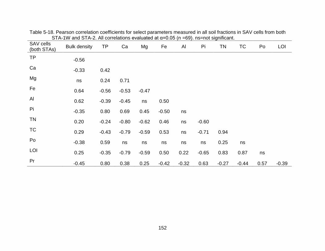
152
Table 5-18. Pearson correlation coefficients for select parameters measured in all soil fractions in SAV cells from both STA-1W and STA-2. All correlations evaluated at α=0.05 (n =69). ns=not significant.
SAV cells (both STAs)
Bulk density TP Ca Mg Fe Al Pi TN TC Po LOI
TP -0.56
Ca -0.33 0.42
Mg ns 0.24 0.71
Fe 0.64 -0.56 -0.53 -0.47
Al 0.62 -0.39 -0.45 ns 0.50
Pi -0.35 0.80 0.69 0.45 -0.50 ns
TN 0.20 -0.24 -0.80 -0.62 0.46 ns -0.60
TC 0.29 -0.43 -0.79 -0.59 0.53 ns -0.71 0.94
Po -0.38 0.59 ns ns ns ns ns 0.25 ns
LOI 0.25 -0.35 -0.79 -0.59 0.50 0.22 -0.65 0.83 0.87 ns
Pr -0.45 0.80 0.38 0.25 -0.42 -0.32 0.63 -0.27 -0.44 0.57 -0.39

153
Table 5-19. Pearson correlation coefficients for select parameters measured in all soil fractions from STA-1W. All correlations evaluated at α=0.05 (n =50). ns=not significant.
STA-1W Bulk density TP Ca Mg Fe Al Pi TN TC Po LOI
TP -0.70
Ca ns 0.46
Mg ns 0.26 0.58
Fe 0.70 -0.68 -0.37 -0.41
Al 0.62 -0.57 ns ns 0.73
Pi -0.36 0.80 0.58 0.44 -0.51 -0.36
TN ns ns -0.45 -0.50 0.24 ns -0.45
TC 0.35 -0.61 -0.67 -0.38 0.47 0.33 -0.66 0.73
Po -0.68 0.80 ns ns -0.49 -0.46 0.50 ns -0.35
LOI 0.40 -0.73 -0.88 -0.51 0.60 0.40 -0.72 0.44 0.80 -0.30
Pr -0.62 0.82 0.31 ns -0.53 -0.55 0.57 ns -0.50 0.63 -0.59

154
Table 5-20. Pearson correlation coefficients for select parameters measured in soil fractions from STA-2. All correlations evaluated at α=0.05 (n =75). ns=not significant.
STA-2 Bulk density TP Ca Mg Fe Al Pi TN TC Po LOI
TP -0.42
Ca ns 0.30
Mg ns ns 0.54
Fe 0.49 -0.51 -0.39 ns
Al 0.55 -0.40 -0.32 ns 0.62
Pi ns 0.75 0.61 0.36 -0.33 ns
TN ns -0.31 -0.79 -0.51 0.38 0.24 -0.65
TC ns -0.51 -0.78 -0.48 0.43 ns -0.75 0.90
Po -0.41 0.77 ns -0.37 -0.33 -0.32 0.28 ns ns
LOI ns -0.34 -0.78 -0.50 0.28 ns -0.65 0.84 0.89 ns
Pr -0.29 0.77 0.35 ns -0.33 -0.25 0.65 -0.32 -0.51 0.56 -0.40

155
Figure 5-1. Location of soil sampling sites in the STAs. Field triplicate sites are shown in red boxes. (Map source –
SFWMD)

156
Figure 5-2. Phosphorus fractionation scheme used to characterize P forms in STA soils.
Modified from Ivanoff and others, (1998).

157
A
B Figure 5-3. Phosphorus fractions (organic [Po], inorganic [Pi] and residual P [Pr]) in floc,
RAS and pre-STA soil in STA-1W. A) Total P content. B) Relative proportion of P fractions.

158
A
B Figure 5-4. Phosphorus fractions (organic [Po], inorganic [Pi] and residual P [Pr]) in floc,
RAS and pre-STA soil in STA-2. A) Total P content. B) Relative proportion of P fractions.

159
Figure 5-5. Inorganic P [Pi] content plotted against TP for all soil sections in EAV and
SAV cells from STA-1W and STA-2.
Figure 5-6. Organic P [Po] content plotted against TP in EAV and SAV cells from STA-
1W and STA-2.

160
Figure 5-7. Percent composition of stable and reactive phosphorus pools in the floc, RAS and pre-STA soil of EAV and SAV cells pooled over both STA-1W and STA-2.

161
Figure 5-8. Non-reactive phosphorus (stable P) as a fraction of total phosphorus in floc,
RAS and pre-STA soil of STA-1W and STA-2.

162
Figure 5-9. Relationship between phosphorus (mg P kg-1) and calcium (g Ca kg-1) in
EAV and SAV cells of STA-1W. Open symbols represent EAV cells and closed symbols represent SAV cells. (n=50). For regression line n= 35, P-value < 0.05.

163
Figure 5-10. Relationship between phosphorus (mg P kg-1) and calcium (g Ca kg-1) in
EAV and SAV cells of STA-2. Open symbols represent EAV cells and closed symbols represent SAV cells. (n=75) For regression line n= 33, P-value < 0.01.

164
CHAPTER 6 CONCLUSIONS
Constructed treatment wetlands are dynamic ecosystems primarily established in
urban or agricultural watersheds to treat nutrient/ contaminant-rich water. These
systems are attractive because of their low cost and ability to provide additional
ecosystem services. Often these systems are evaluated simply by monitoring inflow and
outflow contaminant concentrations, with limited information about the internal
processes regulating contaminant removal, transformation or retention in the system.
The lack of detailed information on nutrient cycling among different wetland
compartments (including water column, plant biomass, surface litter and soil) result in
the ‘black box’ approach that is generally used to evaluate treatment wetland’s
performance (Zurayk and others, 1997). An in-depth understanding of interactions
between the biogeochemical processes responsible for water treatment could aid in
performance optimization, reduction in operational costs, and prediction of future
treatment responses to varied operating conditions.
This dissertation research is one attempt towards advancing our understanding
about the main processes regulating treatment efficiency of constructed wetlands. This
was done by quantifying changes in various nutrient storage pools in soils and using
this information to understand the biogeochemical processes and transformations that
take place in wetland soils. Specifically, by measuring the quantity and chemical stability
of soil phosphorus (P) fractions, the long-term sustainable performance prospect of
treatment wetlands were examined.
Free water surface treatment wetlands located in southern Florida were selected
as the main sites for this study. These wetlands, referred to as the Everglades

165
Stormwater Treatment Areas (STAs), were strategically located in several agricultural
watersheds to remove excess P in surface runoff originating from agricultural farms. In
context of the STAs, understanding the internal processes that regulate treatment
efficiency is of great importance (and urgency) because these systems not only
represent a huge financial investment, but the legally mandated water treatment goals
and the ecological risks to the Everglades of ineffective treatment are very high. By
investigating the storage and movement of P fractions within STA soil layers, an attempt
was made to recognize factors that control and regulate important biogeochemical
processes that affect long-term removal efficiency and P storage in treatment wetlands.
The value of this research is enhanced by the fact that the results can be directly
applied to enhance treatment efficiency of the STAs.
Wetland soils are the main repository of removed nutrients (particularly P),
therefore this dissertation started with quantification of soil nutrient storage pools and
examined how those pools changed over time, and ultimately established relationships
between soil nutrient storage and STA age (Chapter 2). This was followed by
developing a simple change-point technique (CPT) to aid in measuring of soil and P
accretion rates in treatment wetlands (Chapter 3). The boundary between recently
accreted soils (RAS) and pre-STA soil was identified by CPT. Soil accretion rates in
STAs were determined by utilizing depth of RAS layer from the surface and the STA
age where as P mass in RAS was used to calculate P accretion rates. Subsequently, P
mass storages in floc, RAS and pre-STA soil were calculated and P mass balances
were developed for STA-1W, STA-2 and STA-3/4 (Chapter 4). Long-term sustainable P
removal depends on the stability of accreted P, hence chemical characterization of

166
accreted P in STA soils was performed (Chapter 5). In the following sections of this
chapter, each dissertation research objective presented in the Introduction (Chapter 1)
is re-evaluated in the context of the knowledge gained from this research and the goal
of having better understanding of P removal mechanisms in treatment wetlands. This
research was guided by following objectives and supporting hypotheses -
Objective 1: Review available datasets on STA soil physico-chemical variables and determine spatio-temporal changes in surface and sub-surface soil nutrient storage. Explore relationship between hydraulic and water quality parameters, soil nutrient storages and STA age. Perform preliminary P mass balance using these data (Chapter 2).
Hypothesis: STAs’ treatment efficiency or P removal efficiency declines after a protracted period of operation.
Objective 2: Determine the soil accretion rate in the STAs, by utilizing stratigraphic characteristics of the soil profiles to identify the boundary between recently accreted soil (RAS) and antecedent pre-STA soil (Chapter 3).
Hypothesis: The STAs are accreting systems and accumulating organic matter conserves attributes of prevailing conditions (e.g. nutrient loading, vegetation community). Changes in these stratigraphic characteristics can be exploited to identify the depth of RAS deposited on top of pre-STA soil.
Objective 3: Explore the relationship between soil accretion rates and operational age of the STAs. Perform P mass balance using P storages in RAS and pre-STA soil and the amount of P removed from the water column. Determine P cycling within different P storage compartments of the STAs (Chapter 4).
Hypothesis: Most of the P retained from the water column is stored in RAS, which has a higher P concentration than pre-STA soil. With increasing age, the rate of soil and P accretion declines, resulting in higher outflow P concentrations. Internal re-distribution of P within RAS and pre-STA soil is mediated by vegetation. This controls whether the STAs function as a nutrient source or sink.
Objective 4: Determine the relative proportion of reactive and non-reactive P pools in the STAs. Assess the influence of wetlands vegetation communities (EAV vs. SAV) on reactivity of P pools (Chapter 5).
Hypothesis: Different vegetation types (EAV vs. SAV) will influence the proportion of P forms incorporated into RAS and sequestered in the STAs. The presence of more reactive (i.e., potentially mobile) P forms will reduce the long-term sustainability of the STAs.

167
Objective 1: Spatio-Temporal Changes in Soil Nutrient Storages
An inventory of nutrients (P, N and C) stored in STA soils was developed by
reviewing all existing data on floc and soil nutrient storages and subsequently exploring
changes in those pools over time. Phosphorus concentration and storage within various
compartments of the STAs – the water column, floc (unconsolidated detritus), surface
soil (0-10 cm), and sub-surface soil (below 10 cm) were determined. Analysis of the
physico-chemical attributes of STA soils allowed investigation of temporal changes in
nutrient storage and examination of relationships between changes in nutrient storage
with respect to STA performance and operational age (Chapter 2).
Annual P storage rates declined with increasing STA operational age, although
the proportion of P stored in surface soil increasingly came from P retained from the
water column over time. The decline in P storage rates could indicate that accumulation
of refractory organic P fractions in the STAs was not uniform throughout each STA’s
operational history. Continued P loading of the STAs resulted in an increased proportion
of soil P pools being derived from P retained from the water column.
Temporal changes in P storage within the active compartments of the STAs were
used to generate estimates of P flux between these compartments and develop an
overall P mass balance. Over the period of STA operation, it was observed that surface
soils of STAs changed from being a source into net sink for P. However, this analysis
was restricted to P storage within the top 10 cm of surface soil, which may not have
included the entire depth of RAS, hence conclusions drawn from these data are more
akin to ‘best estimates’ of accretion rates and P storages. Subsequently, a more
complete mass balance was developed after identification of the boundary between
RAS and pre-STA soil (Chapter 4).

168
Objective 2: Soil Accretion in Treatment Wetlands
Soil accretion is related to the performance of treatment wetlands as soils
provide a long-term sink for various pollutants. Knowledge of soil accretion rates in the
STAs is important to quantify P mass storages accurately and develop robust mass
balances; however, it was difficult to measure accretion rates in the absence of a
marker horizon. Therefore, a novel analytical technique, CPT, was developed by
exploiting the stratigraphic characteristics of RAS. This allowed for identification of the
boundary between RAS and pre-STA soil, and hence RAS depth in three STAs of
varying age – STA-1W, STA-2 and STA-3/4 (Chapter 3).
Objective 3: Soil Accretion and Operational Age of Treatment Wetlands
Soil accretion is the long-term sustainable mechanism for removal of nutrients
(specifically P in this case) in wetlands; however, it remains the least investigated
component of treatment wetland performance (Kadlec and Wallace, 2009). Changes in
soil accretion rates with increasing operational age of the STAs were evaluated.
Wetland soils aggregate biotic and abiotic processes, hence, results from this study
were useful in understanding some of the biogeochemical processes that control and
regulate P removal in the STAs. Soil and P accretion rates were determined using RAS
depths identified with CPT (Chapter 2). A declining trend in soil and P accretion rates
with increasing age was observed for STA-1W, STA-2 and STA-3/4, which had
operational ages of 16, 11 and 7 years, respectively (Chapter 4). This confirmed the
hypotheses that with increasing age, the rate of soil and P accretion declines.
Developing reliable P mass balances for these wetlands required accurate
estimates of soil accretion rates and associated soil P storages. The ability to
differentiate between P storages in RAS and pre-STA with reasonable confidence

169
allowed calculation of total P flux from pre-STA soil into RAS. The results of P mass
balances developed using this approach are presented in Chapter 4. High P flux from
pre-STA soil to RAS was indicative of the role of vegetation in mining subsurface P and
deposition on the surface through detrital accumulation, which eventually becomes a
part of RAS (Reddy and DeLaune, 2008; Reddy and others, 2002). The movement of P
from pre-STA to RAS layer involved a series of complex biological processes including
growth, senescence and decomposition of wetland vegetation and microbial
assemblages.
Objective 4: Stability of Phosphorus in Recently Accreted Soil
Phosphorus sequestered in wetlands that can be mobilized in response to
changes in nutrient concentration gradients or changes in physical and chemical
conditions (such as redox, electron acceptors and hydrologic regimes) is considered
reactive. Reactive P that becomes bio-available can have adverse ecological impacts. It
therefore was important to investigate the composition and stability of P in RAS to
determine the long-term efficacy of P retention in the STAs.
Chemical characterization of P present in STA soils was carried out using an
operationally defined fractionation scheme modified from Ivanoff and others, (1998).
Phosphorus-enriched STA surface layers (floc and RAS) contained a higher proportion
of reactive P than did pre-STA soil. This reactive pool was comprised of Pi and Po
fractions that together accounted for 65-70% of all TP in floc and RAS. Investigations of
the influence of vegetation type on partitioning of P found significant effect on Pr
fraction. The relative proportion of Pr was lower in EAV cells compared to SAV cells in
STA-1W, whereas no vegetation effect was observed for Pr in STA-2 (Chapter 5).

170
A separate evaluation of floc, RAS and pre-STA soil found that the influence of
vegetation type on P fractions in STA-1W were not significant except for differences in
Po in floc and pre-STA soil. For STA-2, significant differences in P fractions were
observed between EAV and SAV cells for floc (Po), RAS (Pi) and pre-STA soil (Po, Pi
and Pr) (Chapter 5).
Phosphorus mass balances suggested that a large portion of P in RAS was
mined from pre-STA soil. Fractionation analysis indicated that about 70% of P in RAS
was reactive and potentially could be mobilized. This highlights the risk of P loss from
the STAs following changes in the environment (e.g., redox and pH changes, availability
of electron acceptors, etc.). A decline in soil accretion rate was observed with increasing
STA operation age of, which raised an important question regarding continued
performance of the STAs. Without continued high rates of soil accretion, the treatment
performance of the STAs could diminish.
Synthesis
Phosphorus retention pathways in treatment wetlands are comprised of complex
biotic and abiotic processes. This complexity is mainly due to multiple physical,
biological and chemical mechanisms that interact simultaneously to provide treatment.
These reactions result in removal of P from the water column, conversion of
constituents from dissolved to particulate and inorganic to organic forms and vice versa
(Reddy and DeLaune, 2008). Along with these conversions, mobilization of sequestered
P and redistribution of P pools within the soil profile also take place. While P is cycled
through various storage compartments within wetlands, different functional forms of P
undergo transformations (Koch and Reddy, 1992; Newman and Pietro, 2001; Qualls
and Richardson, 2003; Reddy and others, 1999a). Such changes influence the stability

171
of accreted P and overall treatment performance in wetlands. The main goal of this
study was to understand the impacts of operational age, hydraulic and P loading rates,
dominant vegetation type on regulation of the stability of accreted P in treatment
wetlands. These efforts were aimed to understand how these factors may have affected
treatment performance and long-term fate of P in the STAs.
A summary based on the outcomes of this dissertation research at one site (STA
-2) is presented in Figure 6-1 (A= EAV cells and B= SAV cells). This synthesis
highlights the passage that influent P takes as it is removed from the water column and
eventually is stored as accreted soil in EAV and SAV cells The schematic indicates the
partitioning of accreted P into reactive and non-reactive forms within the main storage
compartments of STA soils. Phosphorus loading rates experienced by EAV cells were
slightly lower than in SAV cells for the POR and the annual rate of P retention (water
column to floc) was similar for both vegetation types. However, the annual P accretion
rate to RAS in SAV cells was twice that of EAV cells. Comparison of the proportion of
reactive and non-reactive P in floc, RAS and pre-STA soil found a higher percentage of
reactive P throughout the soil profile. A greater proportion of reactive P (Pi and Po
fractions combined) was observed in the floc and RAS of SAV cells compared to EAV
cells, i.e., floc and RAS of SAV cells contained a larger proportion of P that was prone
to mobilization in response to changes in environmental conditions than in EAV cells.
Positive correlations between TP and Ca in floc and RAS suggested Ca-P co-
precipitation as an important mechanism of P removal in SAV cells. Among reactive P
pools, the proportion of Pi was higher in SAV cells while Po was greater in EAV cells.

172
Residual P comprised 30-35% of TP in floc and RAS of both vegetation types.
Only Pr can be considered as truly removed from the standpoint of future bio-
availability. There is insufficient knowledge regarding the underlying reasons for the
chemical stability of Pr pool in wetlands and further studies are necessary to identify
reasons that impart chemical stability. With advanced scientific techniques such as
nuclear magnetic resonance (NMR) and X-ray Absorption Near Edge Structure
(XANES) absorption spectroscopy, the elemental composition and the structure of the
stable P fraction could possibly be determined (Cheesman and others, 2012). With
regard to continued P removal by STAs, factors that promote the transformation of
retained P into non-reactive forms need to be further investigated.
Future Outlook and Sustainability of STAs
The ecosystems of south Florida are hydrologically linked, beginning from the
headwaters of the Kissimmee River and ending with Florida Bay and the Florida Keys.
Human perturbation has caused many social, economic and environmental impacts on
this system. The impacts of agricultural drainage waters from the Everglades
Agricultural Area (EAA) on the Water Conservation Areas and the southern Everglades
have received much attention, and the six STAs constructed to remedy some of those
problems. STAs represent a huge financial commitment in terms of initial capital costs
and annual operating and management costs. Although, cumulatively the STAs
removed 1500 mt of P (Ivanoff and others, 2012), which otherwise would have
adversely impacted the Everglades ecosystem, there are multiple issues that bring the
long-term sustainability of the STAs and the stability of their sequestered P into
question.

173
First, declining trend in soil and P accretion rates with increasing age as
observed for STA-1W, STA-2 and STA-3/4 is an indicator of slow-down of P removal
rates. With STA age decrease in the quantity of TP retained from the water column
could result in failure to meet legally stipulated outflow P concentration.
Second, an independent economic analysis conducted by the National Research
Council found that the cost of P removal by the STAs is $240 kg-1 (Council, 2011),
which escalates to $600 -$1200 when the proportion of Pr in RAS (30 ± 10 %) is
considered. Such high cost for storage of P in non-reactive fractions may require
greater financial investments, which may not be readily available in the current
economic environment. The environmental risks associated with the potential
mobilization and release of reactive P from the STAs to the downstream Everglades
remains a grave concern.
Third, a vast amount of P exists both in the native soils and has been imported
into the Everglades basin as fertilizer, and the STAs potential to remove P in runoff is
not limitless. The total quantity of P fertilizer applied in the EAA greatly exceeds the
design parameters used to estimate P removal by STAs (Reddy and others, 2011). The
STAs have been loaded with P for many years now and floc and RAS which exist as an
interface with overlying water column have higher TP concentration than pre-STA soil.
Fourth, promotion of best management practices upstream of the STAs may
result in decreasing P concentration in inflow waters, however the introduction of low-P-
concentration water to the STAs could cause P flux from the soil back to the overlying
water column (Reddy and others, 2012).

174
Fifth, south Florida is prone to extreme weather events such as tropical storms
and droughts, and based on recent weather trends, it is not difficult to conclude that the
probability of such events reoccurring in future is high. The existing safe guards against
these extreme events are less than adequate for existing network of six STAs.
Hurricanes have caused considerable damage to vegetation in some STA cells,
necessitating costly rehabilitation efforts to bring those cells back online. STA managers
face increasingly tough challenges to keep STA cells hydrated during summer months
when water demand throughout the District soars. During large rain events when huge
volumes of water pass through STAs scouring channels and negatively impacting
system hydraulics. The flooding situation, however might improve after the construction
of Compartments B and C (Figure 1-3) are completed, which will provide more storage
capacity and control in the timing and volume of flow through the STAs.
Sixth, an action plan once STA’s reach the end of their projected operational life
is missing. One option is to transport STA soil with its sequestered P out of the
Everglades basin, but the economic implications for such action could be very high. If P
is translocated within the basin then it will only delay the ecological consequences
unless adequate measures are taken to prevent remobilization. During years 2005-
2007, rehabilitation of STA-1W resulted in the removal of approximately 180,000 yd3 of
floc and subsurface soils, equivalent to 19 mt of P, in which soil was disposed in a
manner that precluded its P from reaching the Everglades. Some experts have even
suggested reopening the STAs for farming. Recently accreted organic soils with high
quantities of P could serve as productive agricultural soils. Another option is in situ
immobilization by application of specialized chemicals that have high affinity for P.

175
However, these steps can be seen as very practical, particularly when the economics of
implementing these options over the STA’s entire treatment footprint of 18,000 ha.
Although the above mentioned points may seem to suggest a bleak outlook
where long-term sustainability of the STAs is concerned, there are benefits that the
STAs provide. Other than being the best substitute for natural wetlands that were once
part of the historical landscapes, the STAs offer other benefits that go beyond their main
function of P removal. For instance, the STAs provide high quality habitat for fish, birds
and other wildlife and fulfill ecological functions in the landscape. The accreted soil of
STAs sequesters C and N along with P. Calculations for surface soil (10 cm) suggested
that the STAs store thousands of metric tons of C (Chapter 2, Table 2-8). When nutrient
removal costs for both C and N are included in total costs, then the per unit cost of P
removal does not appear so high.
STAs already provide popular recreation activities such as bird watching,
photography, fishing and hunting. The vast amount of data that has been collected from
regular monitoring of the STAs could be mined to enhance the design of interventions
that improve P removal in the STAs and other treatment wetlands. The role of STAs in
reduction of P inputs to the Everglades and the success of Everglades restoration
efforts cannot be overstated. In light of the knowledge gained from this dissertation on
the quantity and quality of sequestered P, further steps can be taken to improve the
efficiency and future of these large treatment wetlands.

176
A
B
Figure 6-1. Summary of total phosphorus (TP) loading rates, TP accretion rates and distribution of reactive and non-reactive TP pools in floc, recently accreted soils (RAS) and pre-STA soil. A) Emergent aquatic vegetation. B) Submerged aquatic vegetation cells of STA-2.

177
APPENDIX A ADDITIONAL DATA AND INFORMATION PERTAINING TO CHAPTER 1
Table A-1. Treatment Wetland Technology conferences. Source: (Kadlec and Wallace, 2009)
Year Location Title (Proceedings)
1976 Ann Arbor, Michigan
Freshwater Wetland and Sewage Effluent Disposal
1978 Tallahassee, Florida
Environmental Quality Through Wetlands Utilization
1978 Lake Buena Vista, Florida
Wetland Functions and Values
1979 Higgins Lake, Michigan
Freshwater Wetland and Sanitary Wastewater Disposal
1979 Davis, California Aquaculture Systems for Wastewater Treatment
1981 St. Paul, Minnesota
Wetland Values and Management
1982 Amherst, Massachusetts
Ecological Considerations in Wetlands Treatment of Municipal Wastewaters
1986 Orlando, Florida Aquatic Plants for Water Treatment and Resource Recovery
1988 Chattanooga, Tennessee
1st International Conference on Constructed Wetlands for Wastewater Treatment
1989 Tampa, Florida Wetlands: Concerns and Successes
1990 Cambridge, United Kingdom
2nd International Conference on Constructed Wetlands for Water Pollution Control
1991 Pensacola, Florida
Constructed Wetlands for Water Quality Improvement
1992 Columbus, Ohio INTECOL Wetlands Conference
1992 Sydney, Australia
3rd International Conference on Wetland Systems for Water Pollution Control
1994 Guangzhou, China
4th International Conference on Wetland Systems for Water Pollution Control
1994 Atlanta, Georgia On-Site Wastewater Treatment; 7th Symposium on Individual and Small Community Sewage Systems
1995 Třeboń, Czech Republic
Nutrient Cycling and Retention in Wetlands and Their Use for Wastewater Treatment
1996 Vienna, Austria 5th International Conference on Wetland Systems for Water Pollution Control
1996 Niagara-on-the-Lake, Ontario
Constructed Wetlands in Cold Climates
1997 Romulus, Michigan
Constructed Wetlands for the Treatment of Landfill Leachates

178
Table A-1. Continued.
Year Location Title (Proceedings)
1997 Třeboń, Czech Republic
Nutrient Cycling and Retention in Natural and Constructed Wetlands
1998 Aguas de São Pedro, Brazil
6th International Conference on Wetland Systems for Water Pollution Control
1998 Orlando, Florida On-Site Wastewater Treatment; 8th Symposium on Individual and Small Community Sewage Systems
1999 Salt Lake City, Utah
Wetlands and Remediation
1999 Třeboń, Czech Republic
Transformations of Nutrients in Natural and Constructed Wetlands
1999 Baltimore, Maryland
Wetlands for Wastewater Recycling
1999 Tartu, Estonia Constructed Wetlands for Wastewater Treatment in Cold Climates
2000 Quebec, Canada
INTECOL Wetlands Conference
2000 Orlando, Florida 7th International Conference on Wetland Systems for Water Pollution Control
2001 Burlington, Vermont
Wetlands and Remediation II
2001 Třeboń, Czech Republic
Wetlands: Nutrients, Metals, and Mass Cycling
2001 Fort Worth, Texas
On-Site Wastewater Treatment: 9th Symposium on Individual and Small Community Sewage Systems
2002 Dar es Salaam, Tanzania
8th International Conference on Wetland Systems for Water Pollution Control
2003 Borová Lada, Czech Republic
Natural and Constructed Wetlands: Nutrients, Metals, and Management
2003 Tartu, Estonia Constructed and Riverine Wetlands for Optimal Control of Wastewater at Catchment Scale
2003 Lisbon, Portugal The Use of Aquatic Macrophytes for Wastewater Treatment in Constructed Wetlands
2004 Wexford, Ireland
Nutrient Management in Agricultural Watersheds: A Wetlands Solution
2004 Avignon, France 9th International Conference on Wetland Systems for Water Pollution Control
2005 Ghent, Belgium 1st Wetland Pollutant Dynamics and Control (WETPOL)
2006 Třeboń, Czech Republic
Wastewater Treatment, Plant Dynamics, and Management in Constructed and Natural Wetlands
2006 Lisbon, Portugal 10th International Conference on Wetland Systems for Water Pollution Control
2007 Padua, Italy Multi-Functions of Wetland Systems
2007 Tartu, Estonia 2nd Wetland Pollutant Dynamics and Control

179
APPENDIX B ADDITIONAL DATA AND INFORMATION PERTAINING TO CHAPTER 2
STA Description
Stormwater Treatment Area 1 East (STA-1E) is located northeast of the Arthur
R. Marshall Loxahatchee National Wildlife Refuge (LNWR) in Palm Beach County, FL
and began operation in WY2005. This STA has three flow-ways (East, Central, and
West) covering approximately 2,104 ha. STA-1E has been adversely affected by high
hydraulic loading during storm events (in WY2006), water control structure failures,
topographic issues (Cells 5 and 7), dryout of cells during regional drought (WY2009)
and vegetation die-off. Through WY2012, STA-1E has treated over 600,000 ac-ft of
water and retained approximately 94 mt of TP (Ivanoff and others, 2012). The period-of-
record (POR) inflow flow-weighted mean (FWM) TP concentration was 176 µg L-1, while
the POR outflow FWM TP concentration was 57 µg L-1 (Ivanoff and others, 2012).
Stormwater Treatment Area 1 West (STA-1W) began operation in WY1995
and is located northwest of the Arthur R. Marshall LNWR. It has three flow-ways totaling
2,700 ha of effective treatment area: East (Cells 1A, 1B and 3), West (Cells 2A, 2B and
4), and North (Cells 5A and 5B). The East and West Flow-ways were formerly known as
the Everglades Nutrient Removal Project; the North Flow-way was added in WY2000.
Cells 1 and 2 were reconfigured in WY2007, creating Cells 1A, 1B, 2A and 2B.
Supplemental water has been delivered from Lake Okeechobee to maintain hydration
during dry months. To date, STA-1W has treated over 3.3 million ac-ft of water and
retained approximately 480 mt of TP (Ivanoff and others, 2012). The POR mean inflow
FWM TP concentration was 171 µg L-1, while the POR mean outflow FMW TP
concentration was 51 µg L-1 (Ivanoff and others, 2012). Over its period of operation,

180
STA-1W has been impacted by extreme weather events (regional droughts and tropical
storms), construction activities, and high hydraulic and nutrient loadings. STA-1W
underwent a substantial rehabilitation and enhancement effort during 2005-2007.
Approximately 180,000 yd3 of P-enriched floc and surface soil were removed from Cells
1B and 4. This resulted in a total removal of 19 mt P from STA-1W. The WY2007 soil
phosphorus storage (SPS) values in Table 2-9 reflect P storage before soil removal,
while soil samples collected in WY2008 represent post-rehabilitation SPS. The
observed decrease in SPS in the later samples could be attributed to the rehabilitation
activities.
Stormwater Treatment Area 2 (STA-2) is located in western Palm Beach
County immediately west of WCA-2A. STA-2 originally consisted of three one-cell flow-
ways (Cells 1, 2 and 3) with a combined 2,565 ha of effective treatment area and began
operation in the WY2000. The treatment area was expanded by 770 ha with the
construction of Cell 4, which became operational in December 2006. Compartment B
construction will add approximately 2,760 ha of additional treatment area to STA-2.
From WY2000–WY2012, STA-2 has treated over 2.8 million ac-ft of water and retained
approximately 269 mt of TP (Ivanoff and others, 2012). The POR inflow FWM TP
concentration was 102 µg L-1 while the POR outflow FWM TP concentration was 22 µg
L-1 (Ivanoff and others, 2012).
Stormwater Treatment Area 3/4 (STA-3/4) is located northeast of the Holey
Land Wildlife Management Area and north of WCA-3A. It has a total treatment area of
6,691 ha and receives runoff originating within the S-2/7, S-3/8, S-236 and C-139
basins and water releases from Lake Okeechobee. STA-3/4 has three flow-ways: East

181
(Cells 1A and 1B), Central (Cells 2A and 2B) and West (Cells 3A and 3B). Since it
began operation in October 2003, STA-3/4 has treated approximately 3.7 million ac-ft of
runoff, retaining over 440 mt of TP, and reducing the FWM TP concentration from 114
µg L-1 at the inflow to 18 µg L-1 at the outflow (Ivanoff and others, 2012). Similar to the
other STAs, STA-3/4 has been impacted by extreme weather events (regional droughts
and tropical storms) and high hydraulic loadings during the wet season. The WY2011
dry season resulted in a complete dry out of all cells in STA-3/4 in June 2011.
Stormwater Treatment Area 5 (STA-5) totals 2,465 ha and is located west of
Rotenberger wildlife management area. It is divided into three west-to-east oriented
flow-ways each with two cells. STA-5 began operation in WY1999. Since WY2000,
STA-5 has treated over 1.2 million ac-ft of runoff water and retained approximately 212
mt of TP. The POR inflow FWM TP was 225 µg L-1 and the POR outflow FWM TP
concentration was 93 µg L-1 (Ivanoff and others, 2012). Over its period of operation,
STA-5 has been impacted by high inflow nutrient concentrations and extreme weather
events (regional droughts and tropical storms).
Stormwater Treatment Area 6 (STA-6) is the smallest of the six STAs with a
footprint of 915 ha. It is divided into three east-to-west oriented flow-ways each with only
one cell. The two southernmost cells - Cells 3 and 5 comprise Section 1 while the
northern Section 2 has only Cell 2 which was added in WY2007. The completion of
Compartment C construction will connect STA-5 and STA-6 and they may be identified
as STA-5/6 in the future. The POR inflow TP FWM concentration in STA-6 was 100 µg
L-1 and POR outflow FMW TP concentration was 34 µg L-1 (Ivanoff and others, 2012).

182
Table B-1. Mean total nitrogen concentration in floc and soils in STAs (g N kg-1; mean ± 1 SD). Values represent entire floc depth and the top 10 cm of surface soil.
WY STA-1E STA-1W STA-2 STA-3/4 STA-5 STA-6
Floc*
2003 -- -- -- -- 30 ± 5 --
2007 15.1 ± 0* 23 ± 2 14 ± 3 18 ± 2 28 ± 2 --
Soil
1995 -- 28 ± 2 -- -- -- --
1996 -- 32 ± 4 -- -- -- --
2000 -- 30 ± 3 -- -- -- --
2001 -- -- 3 ± 0 -- 26 ± 6 13 ± 3
2003 -- -- -- -- 22 ± 7 --
2004 -- 28 ± 3 28 ± 3 -- 23 ± 7 21 ± 6
2005 5.9 ± 5.1 -- -- 26 ± 5 -- --
2006 -- 27 ± 3 -- -- -- --
2007 5.6 ± 4.8 26 ± 7 28 ± 2 25 ± 5 21 ± 6 --
2008 -- 28 ± 4 -- -- -- -- #Total nitrogen concentration for floc was not available for STAs 1W, 2, 5 and 6 during WY2004.

183
Table B-2. Mean total carbon concentration in floc and soils in STAs (g C kg-1; mean ± SD). Values represent entire floc depth and the top 10 cm of surface soil.
Year STA-1E STA-1W STA-2 STA-3/4 STA-5 STA-6
Floc*
2003 -- -- -- -- 389 ± 56 --
2007 -- 274 ± 13 242 ± 32 275 ± 22 375 ± 28 --
Soil
1995 -- 360 ± 12 -- -- -- --
1996 -- 510 ± 46 -- -- -- --
2000 -- 483 ± 40 -- -- -- --
2001 -- -- 466 ± 9 -- 381 ± 80 169 ± 46
2003 -- -- -- -- 312 ± 91 --
2004 -- 467 ± 47 419 ± 55 -- 322 ± 102 266 ± 79
2005 87 ± 76 -- -- 391 ± 85 -- --
2006 -- 450 ± 38 -- -- -- --
2007 82 ± 71 398 ± 69 452 ± 38 381 ± 79 297 ± 94 --
2008 -- 450 ± 60 -- -- -- -- #Total carbon concentration for floc was not available for STA- 1W, 2, 5 and 6 during WY2004.

184
Table B-3. STA performance for WY2011 (May 1, 2010–April 30, 2011) and the period of record (POR) 1994–2011. Source: (Ivanoff and others, 2012)
STA-1E STA-1W STA-2 STA-3/4 STA-5 STA-6 All STAs
Effective Treatment Area in Permit (acres) 5,132 6,670 8,240 16,543 6,095 2,257 44,937
Adjusted Effective Treatment Area (acres)a 4,881 6,670 7,406 16,543 5,660 1,584 42,744
Rainfall
Total Annual Rainfall (inches) 34.0b 35.0b 38.1 40.2 39 42.2b 38.1
South Florida Water Management Model (SFWMM) Simulation Rainfall Range (inches)
39.8–77.5 36.6–77.4 35.4–71.6 32.3–70.7 38.6–61.4 46.8–57.6 ---
Inflow
Total Inflow Volume [acre-feet (ac-ft)] 35,616 125,933 170,838 303,447 26,609 72,722 735,165
Total Inflow total phosphorus (TP) Load [metric ton (mt)]
4.955 23.461 15.248 26.208 5.258 10.141 85.271
Flow-weighted Mean (FWM) Concentration Inflow TP [parts per billion (ppb)]
113 151 72 70 160 113 94
Hydraulic Loading Rate (HLR) [centimeters per day (cm/d)
d
0.61 1.58 1.93 1.53 0.39 3.83 1.44
TP Loading Rate (PLR) [grams per square meter per year (g/m
2/yr)]
d
0.25 0.87 0.51 0.39 0.23 1.58 0.49
Outflow
Total Outflow Volume (ac-ft) 25,758 126,881 159,914 312,067 24,319 74,591 723,530
Total Outflow TP Load (mt) 0.691 3.99 3.049 6.305 1.42 2.317 17.772
FWM Concentration Outflow TP (ppb) 22 25 15 16 47 25 20
Outflow Plus Diversion Structures FWM TP (ppb) 22 25 15 17 47 25 20
Hydraulic Residence Time (days) 49 27 23 28 13 5 ---
TP Retained (mt) 4.264 19.471 12.199 19.903 3.838 7.824 67.499
TP Removal Rate (g/m2/yr) 0.22 0.72 0.41 0.3 0.17 1.22 0.39
Load Reduction (percent) 86% 83% 80% 76% 73% 77% 79%
Period of Record Performance
Start Date Sep-04 Oct-93 Jun-99 Oct-03 Oct-99 Oct-97 1994–2011
Total Inflow Volume (ac-ft) 563,131 3,160,086 2,568,599 3,369,553 1,182,264 671,380 11,515,014
Total TP Load Retained to Date (mt) 84.469 465.434 250.619 400.612 205.029 64.132 1,470.30
FWM Concentration TP Outflow to Date (ppb) 62 52 23 17 95 33 38

185
Table B-3. Continued.
a Adjusted effective treatment areas (AETA) reflect treatment cells temporarily off-line for plant rehabilitation, infrastructure repairs, or
Long-Term Plan (LTP) enhancements (see Table 5-4 in Volume I, Chapter 5 for more information about the operational status of the STAs). AETA = # days online/365 (for each flow-way or cell) * (effective treatment area for each flow-way or cell) then add the AETAs for all cells in each STA.
b The total annual rainfall received by the STA was below the range of values used to develop the interim effluent limits (IELs).
c SFWMM – South Florida Water Management Model.
d Inflow volume or TP load/adjusted effective treatment area.

186
APPENDIX C ADDITIONAL DATA AND INFORMATION PERTAINING TO CHAPTER 3
Table C-1. Number of 2-cm sections produced by sectioning soil cores collected from sampling locations in STA-1W. (Total 733 core sections)
Cell 1A 129 Cell 2A 78 Cell 3 97 Cell 5A 86
1B# 15 2F 19 3B 24 5A112 16
1B(i) 23 2Q 18 3I 21 5A112(a) 18
1I 24 2Q(a) 20 3I(a) 16 5A112(b) 16
1I (a)* 22 2Q(b) 21 3I(b) 17 5A150 17
1I (b)* 23 - - 3P 19 5A74 19
1P 22 - - - - - -
Cell 1B 85 Cell 2B 70 Cell 4 74 Cell 5B 114
1AB 12 2AB 17 4C 13 5B 108 21
1AB(a) 19 2U 16 4F 16 5B 125 12
1AB(b) 16 2U(a) 18 4F(a) 14 5B 125(a) 14
1AE 17 2U(b) 19 4F(b) 16 5B 125(b) 14
1T 21 - - 4J 15 5B 162 19
- - - - - - 5B 202 18
- - - - - - 5B 83 16
# This site was located in a canal so another soil core [1B(i)] was collected 3 m away from the canal. *(a) and (b) indicate replicate soil cores collected from this site.
Table C-2. Number of 2-cm sections produced by sectioning soil cores collected from
sampling locations in STA-2..(Total 505 core sections)
Cell 1 106 Cell 2 201 Cell 3 105 Cell 4 93
A103 20 B117 22 C129 18 D111 8
A103 (a)* 15 B151 20 C165 15 D124 19
A103 (b)* 20 B187 20 C201 16 D124 (a) 15
A138 21 B26 17 C21 13 D124 (b) 21
A172 16 B31 23 C75 18 D129 18
A51 14 B31(a) 22 C75 (a) 16 D139 12
- - B81 22 C75 (b) 9 - -
- - B98 14 - - - -
- - B98(a) 21 - - - -
- - B98(b) 20 - - - -

187
Table C-3. Number of 2-cm sections produced by sectioning soil cores collected from sampling locations in STA-3/4. (Total 573 core sections)
Cell 1A 138 Cell 1B 177 Cell 2A 133 Cell 2B 125
1A-19~ 2 1B-24 9 2A-1 19 2B-13 8
1A-21 11 1B-28 13 2A-12 7 2B-17 6
1A-3 8 1B-4 10 2A-16 13 2B-17(a) 7
1A-32 11 1B-52 6 2A-24 5 2B-17(b) 7
1A-32 (a)* 12 1B-52(a) 12 2A-24(a) 7 2B-21 11
1A-32 (b)* 14 1B-52(b) 7 2A-24(b) 6 2B-24 16
1A-36 6 1B-56 17 2A-28 4 2B-28 8
1A-48 14 1B-60 19 2A-28(a) 5 2B-3 7
1A-52 9 1B-60(a) 20 2A-28(b) 5 2B-40 8
1A-52(a) 8 1B-60(b) 17 2A-38 9 2B-44 8
1A-52(b) 8 1B-8 7 2A-42 7 2B-44(a) 11
1A-56 10 1B-80 17 2A-5 13 2B-44(b) 12
1A-7 9 1B-84 12 2A-53 14 2B-55 8
1A-71 9 1B-87 11 2A-53(a) 3 2B-59 8
1A-74 7 - - 2A-57 16 - -
~ Soil cores too short to be considered for analysis * (a) and (b) depicts two replicates collected from same site.

188
Figure C-1. Soil core sampling locations in each cell of STA-1W. (Base map source: SFWMD).

189
Figure C-2. Soil core sampling locations in each cell of STA-2. (Base map source: SFWMD).

190
Figure C-3. Soil core sampling locations in each cell of STA-3/4.(Base map source: SFWMD).

191
APPENDIX D ADDITIONAL DATA AND INFORMATION PERTAINING TO CHAPTER 4
Soil Profiles - Difference between Operational Cells
STA-1W
Soil physico-chemical parameters along the soil profile were averaged over each
2-cm strata in all soil cores from each cell of STA-1W (Figure D-1). Since not all cells in
STA-1W became operational at the same time, differences in cell age and could be
responsible for the variability observed in different parameters. Cells 2B and 4
underwent significant rehabilitation work during WY 2006-2007, including tilling and
removal of surface soil, therefore soil δ15N (‰) and δ13C (‰) values for soil cores from
these two cells were not determined.
Higher bulk density in the top layers of Cells 4 and 2B (Figure D-1 (a)) could be a
result of compaction from earth-moving equipment used during rehabilitation activities,
or consolidation and compaction caused by other processes. The concentration of TP
was highest on the surface and showed decrease with increasing depth in all STA-1W
cells (Figure D-1 (b)). This could be attributable to the fact that surface soil layer
interacts with the overlying water column, periphyton and floc, and often serve as a
major repository of P inputs to the system, while deeper soil layers experience P
depletion as a result of P mining by plants.
Except for Cell 1B, all cells in STA-1W showed greater values for δ15N (‰) in the
upper soil layers (approximately 10-12 cm) relative to deeper sections (Figure D-1 (c)).
Cells 3 and 1A showed δ13C (‰) greater values in the top soil layers whereas Cells 1B
and 5A showed lesser enrichment near the soil surface (Figure D-1(d)). In comparison
to other cells, Cell 5B (SAV) showed decrease in the δ13C (‰) values. The average soil

192
C:N ratio in all cells of STA-1W was relatively constant with depth (Figure D-1 (e)).
However, average N:P ratio of soil cores in STA-1W showed an increasing trend with
depth (Figure D-1 (f)).
STA-2
Various physico-chemical parameters along soil profile were averaged over each
2-cm strata in all soil cores collected from each cell of STA-2 (Figure D-2). Cells 1, 2
and 3 had been in operation since WY2000 while Cell 4 was still in its stabilization
phase as late as WY2007 (3 years before soil sampling). Differences in cell age could
account for some of the variability in various parameters among the cells.
Bulk density was low in the top soil layers, which increased in deeper layers
(Figure D-2 (a)). Cell 1 and 2 had considerably lower bulk density at depth compared to
Cells 3 and 4. Total P decreased with depth. This could be attributable to the fact that
surface soil layer interacts with the overlying water column, periphyton and floc, and
often serve as a major repository of P inputs to the system, while deeper soil layers
experience P depletion as a result of P mining by plants (Figure D-2 (b)). Total P in
surface layers was relatively higher in Cells 1 and 2 (EAV) compared to Cells 3 and 4
(SAV). All cells of STA-2 had higher δ15N (‰) values in the top 10-12 cm of soil (Figure
D-2 (c)). However, only the top soil layers of Cells 3 and 4 (SAV cells) exhibited greater
δ13C (‰) whereas Cells 1 and 2 (EAV cells) did not show this trend (Figure D-2 (d)).
The reason for divergent trend in δ13C (‰) values for EAV and SAV cells can be
attributed to differences in C processing by different vegetation types in these cells. The
C:N mass ratio was relatively constant with increasing depth across all cells (Figure D-2
(e)). However, N:P ratios in Cells 1 and 2 showed a consistent increasing trend with the

193
depth while Cells 3 and 4 exhibited a decreasing N:P ratio after 20-25-cm (Figure D-2
(f)). The varying trends seen in the deeper soil depths could reflect past land use prior
to the establishment of the STAs.
STA-3/4
Variation with depth among different soil physico-chemical parameters in all soil
cores collected from STA-3/4 is shown in Figure D-3. Cell 1B functioned as an EAV cell
for most of its operational history before it was converted to SAV cell in WY2008. Soil
sampling was carried out WY2010. Therefore, the variability observed in surface soil in
this cell may be a result of changed vegetation as a consequence of new hydroperiod.
Bulk density showed a consistent increasing trend with soil depth in all cells
except for a small increase around 19-21 cm (Figure D-3 (a)). Cell 1B had lower bulk
density compared to Cells 1A, 2A and 2B. Total P decreased with depth with relatively
higher TP values in the surface layers Cells 1A and 2A (EAV) than in Cells 1B and 2B
(SAV) (Figure D-3 (b)). Cells 1A and 2A were enriched for heavier δ15N (‰) in the top
soil layers down to 8 cm, below which the soils from all four cells had similar δ15N (‰)
content (Figure D-3 (c)). Cells 1A, 2A and 2B had greater δ13C (‰) values in the surface
layers, whereas Cell 1B showed no increase in δ13C (‰) values in the top soil sections
(Figure D-3 (d)). Carbon:nitrogen mass ratios were relatively uniform with depth across
all cells (Figure D-3 (e)). However, N:P ratio, in all cells generally increased with depth
(Figure D-3 (f)) although the N:P ratio in cells 2A and 2B decreased after 27 cm and 21
cm depth, respectively.

194
Table D-1. STA-1W soil core collection sites by vegetation type and cell. A total of 41 soil cores were collected from these locations.
EAV EAV EAV SAV SAV SAV EAV Conversion
Cell 1A Cell 2A Cell 5A Cell 2B Cell 4 Cell 5B Cell 3 Cell 1B
1B# 2F 5A112 2AB 4C 5B108 3B 1AB
1B(i) 2Q 5A112(a) 2U 4F 5B125 3I 1AB(a)
1I 2Q(a) 5A112(b) 2U(a) 4F(a) 5B125(a) 3I(a) 1AB(b)
1I (a)* 2Q(b) 5A150 2U(b) 4F(b) 5B125(b) 3I(b) 1AE
1I (b)* - 5A74 - 4J 5B202 3P 1T
1P - - - - 5B83 - -
- - - - - 5B162 - -
#This site was located in a canal so another soil core (1B(i)) was collected 3 m away from the canal. *(a) and (b) indicate replicate soil cores collected from this site.
Table D-2. STA-2 soil core collection sites by vegetation type and cell. A total of 29 soil cores were collected from these locations.
EAV EAV SAV SAV
Cell 1 Cell 2 Cell 3 Cell 4
A103 B117 C129 D111
A103(a)* B151 C165 D124
A103(b)* B187 C201 D124(a)
A138 B26 C21 D124(b)
A172 B31 C75 D129
A51 B31(a) C75(a) D139
- B81 C75(b) -
- B98 - -
- B98(a) - -
- B98(b) - -
* (a) and (b) signify replicate soil cores collected from this site.

195
Table D-3. STA-3/4 soil core collection sites by vegetation type and cell. A total 58 soil cores were collected from these locations.
EAV EAV SAV SAV
Cell 1A Cell 2A Cell 1B Cell 2B
1A-19 2A-1 1B-24 2B-13
1A-21 2A-12 1B-28 2B-17
1A-3 2A-16 1B-4 2B-17(a)
1A-32 2A-24 1B-52 2B-17(b)
1A-32(a)* 2A-24(a) 1B-52(a) 2B-21
1A-32(b)* 2A-24(b) 1B-52(b) 2B-24
1A-36 2A-28 1B-56 2B-28
1A-48 2A-28(a) 1B-60 2B-3
1A-52 2A-28(b) 1B-60(a) 2B-40
1A-52(a) 2A-38 1B-60(b) 2B-44
1A-52(b) 2A-42 1B-8 2B-44(a)
1A-56 2A-5 1B-80 2B-44(b)
1A-7 2A-53 1B-84 2B-55
1A-71 2A-53(a) 1B-87 2B-59
1A-74 2A-57 - -
* (a) and (b) signify replicate soil cores collected from this site.

196
Table D-4. Summary statistics for change point depths calculated with SegReg in soil cores collected from STA-1W, STA-2 and STA-3/4.
EAV EAV EAV SAV SAV SAV EAV conversion
STA 1W Cell 1A Cell 2A Cell 5A# Cell 2B Cell 1B Cell 4 Cell 3 Cell 5B#
Sites (n) 5 4 5 4 5 5 5 7
Mean (cm) 19.3 16.7 10.4 15.8 13.5 10.8 12.9 12.4
Standard deviation
(cm)
7.3 1.5 4.2 5.4 2.7 3.5 4.8 6.5
CV* (%) 38 9 40 34 20 32 37 52
STA-2 Cell 1 Cell 2 Cell 3 Cell 4 -- --
Sites (n) 6 10 7 6 -- --
Mean (cm) 8.9 10.4 12.5 12.9 -- --
Standard deviation
(cm)
1.8 2.6 4 3.8 -- --
CV* (%) 20 25 32 29 -- --
STA-3/4 Cell 1A Cell 2A Cell 1B Cell 2B -- --
Sites (n) 10 6 13 10 -- --
Mean (cm) 8.2 11.9 12.1 8.4 -- --
Standard deviation
(cm) 2.9 6.7 5 2.8 -- --
CV* (%) 35 56 41 33 -- --
* Coefficient of variation
# Cell 5A and 5B went online in WY2000, while the other cells in STA-1W started operation in WY1994.

197
Table D-5. Bulk density profiles in soil cores collected from each cell of STA-1W
Depth Mean bulk density (g cm-3) ± 1 SD
(cm) Cell 1A Cell 1B Cell 2A Cell 2B Cell 3 Cell 4 Cell 5A Cell 5B
-1 0.19 ± 0.09 0.31 ± 0.02 0.11 ± 0.05 0.29 ± 0.06 0.2 ± 0.04 0.34 ± 0.07 0.21 ± 0.14 0.23 ± 0.04
-3 0.22 ± 0.07 0.35 ± 0.07 0.16 ± 0.06 0.31 ± 0.04 0.21 ± 0.05 0.37 ± 0.09 0.32 ± 0.25 0.3 ± 0.03
-5 0.24 ± 0.06 0.33 ± 0.02 0.18 ± 0.06 0.34 ± 0.06 0.23 ± 0.06 0.45 ± 0.06 0.42 ± 0.26 0.32 ± 0.04
-7 0.27 ± 0.03 0.3 ± 0.04 0.24 ± 0.04 0.36 ± 0.04 0.27 ± 0.07 0.44 ± 0.06 0.4 ± 0.08 0.31 ± 0.07
-9 0.25 ± 0.06 0.27 ± 0.06 0.26 ± 0.04 0.36 ± 0.03 0.33 ± 0.05 0.44 ± 0.08 0.37 ± 0.07 0.33 ± 0.11
-11 0.25 ± 0.01 0.28 ± 0.09 0.28 ± 0.02 0.38 ± 0.02 0.34 ± 0.06 0.43 ± 0.07 0.34 ± 0.08 0.28 ± 0.07
-13 0.25 ± 0.03 0.28 ± 0.07 0.31 ± 0.03 0.38 ± 0.04 0.35 ± 0.03 0.4 ± 0.03 0.33 ± 0.11 0.29 ± 0.1
-15 0.28 ± 0.01 0.31 ± 0.08 0.33 ± 0.03 0.37 ± 0.06 0.33 ± 0.05 0.37 ± 0.03 0.33 ± 0.09 0.28 ± 0.11
-17 0.26 ± 0.03 0.31 ± 0.06 0.33 ± 0.02 0.35 ± 0.03 0.35 ± 0.05 0.36 ± 0.03 0.32 ± 0.1 0.29 ± 0.09
-19 0.25 ± 0.04 0.28 ± 0.07 0.35 ± 0.03 0.35 ± 0.01 0.36 ± 0.05 0.36 ± 0.04 0.32 ± 0.07 0.27 ± 0.11
-21 0.24 ± 0.05 0.26 ± 0.04 0.37 ± 0.04 0.36 ± 0.08 0.35 ± 0.04 0.32 ± 0.05 0.3 ± 0.1 0.27 ± 0.08
-23 0.24 ± 0.07 0.26 ± 0.08 0.36 ± 0.03 0.31 ± 0.05 0.35 ± 0.02 0.31 ± 0.07 0.3 ± 0.11 0.26 ± 0.06
-25 0.23 ± 0.09 0.26 ± 0.07 0.34 ± 0.08 0.28 ± 0.08 0.33 ± 0.07 0.23 ± 0.05 0.29 ± 0.12 0.25 ± 0.08
-27 0.21 ± 0.07 0.24 ± 0.01 0.33 ± 0.08 0.25 ± 0.07 0.32 ± 0.07 0.23 ± 0.09 0.26 ± 0.1 0.23 ± 0.06
-29 0.19 ± 0.07 0.22 ± 0.06 0.34 ± 0.11 0.22 ± 0.05 0.29 ± 0.08 0.23 ± 0.09 0.26 ± 0.09 0.19 ± 0.03
-31 0.18 ± 0.06 0.19 ± 0.01 0.32 ± 0.1 0.22 ± 0.06 0.27 ± 0.08 -- 0.24 ± 0.09 0.17 ± 0.04
-33 0.18 ± 0.06 0.18 ± 0.06 0.26 ± 0.06 0.19 ± 0.05 0.32 ± 0.1 -- 0.17 ± 0.03 0.17 ± 0.02
-35 0.15 ± 0.03 0.24 ± 0.1 0.22 ± 0.06 -- 0.27 ± 0.05 -- -- 0.16 ± 0.04
-37 0.14 ± 0.02 0.16 ± 0.02 0.2 ± 0.02 -- 0.19 ± 0.04 -- -- --
-39 0.13 ± 0.01 -- 0.19 ± 0 -- 0.22 ± 0.05 -- -- --
-41 0.12 ± 0.02 -- -- -- 0.19 ± 0.01 -- -- --
-43 0.13 ± 0.03 -- -- --
-- -- --

198
Table D-6. Total phosphorus profiles in soil cores collected from each cell of STA-1W
Depth Mean total phosphorus (mg/kg) ± 1 SD
(cm) Cell 1A Cell 1B Cell 2A Cell 2B Cell 3 Cell 4 Cell 5A Cell 5B
-1 1033 ± 455 435 ± 129 1475 ± 245 729 ± 242 802 ± 219 542 ± 95 1085 ± 437 941 ± 256
-3 811 ± 343 365 ± 119 1209 ± 304 525 ± 68 744 ± 281 557 ± 113 769 ± 398 714 ± 164
-5 672 ± 381 296 ± 164 1074 ± 216 533 ± 113 744 ± 336 405 ± 55 482 ± 200 570 ± 156
-7 562 ± 423 277 ± 164 868 ± 325 554 ± 68 449 ± 199 398 ± 81 442 ± 167 412 ± 117
-9 469 ± 443 297 ± 224 704 ± 249 455 ± 124 346 ± 260 338 ± 114 378 ± 147 401 ± 116
-11 466 ± 406 341 ± 340 590 ± 130 382 ± 120 265 ± 117 280 ± 117 373 ± 163 374 ± 108
-13 452 ± 364 211 ± 44 420 ± 45 387 ± 115 231 ± 65 217 ± 32 332 ± 108 388 ± 200
-15 345 ± 86 205 ± 40 364 ± 54 361 ± 111 213 ± 46 211 ± 23 273 ± 67 353 ± 173
-17 250 ± 14 187 ± 23 466 ± 296 354 ± 110 203 ± 37 199 ± 11 260 ± 78 336 ± 174
-19 220 ± 10 180 ± 15 299 ± 37 390 ± 136 204 ± 41 192 ± 11 262 ± 82 325 ± 194
-21 203 ± 17 168 ± 23 309 ± 36 354 ± 110 200 ± 43 189 ± 14 237 ± 81 299 ± 159
-23 190 ± 18 168 ± 29 298 ± 36 313 ± 114 199 ± 31 180 ± 21 222 ± 117 295 ± 138
-25 177 ± 23 168 ± 31 272 ± 67 235 ± 109 190 ± 48 174 ± 19 229 ± 117 263 ± 70
-27 174 ± 22 155 ± 18 259 ± 95 195 ± 101 185 ± 40 160 ± 26 212 ± 114 263 ± 141
-29 169 ± 16 130 ± 26 255 ± 95 165 ± 85 180 ± 45 163 ± 21 216 ± 126 198 ± 46
-31 165 ± 10 110 ± 19 240 ± 90 166 ± 86 171 ± 53 -- 165 ± 106 156 ± 28
-33 165 ± 19 113 ± 42 207 ± 67 147 ± 25 193 ± 44 -- 77 ± 14 144 ± 22
-35 161 ± 8 140 ± 58 192 ± 64 -- 174 ± 41 -- -- 136 ± 20
-37 153 ± 18 106 ± 11 133 ± 29 -- 149 ± 36 -- -- --
-39 149 ± 23 -- 130 ± 0 -- 140 ± 14 -- -- --
-41 160 ± 10 -- -- -- 167 ± 34 -- -- --
-43 155 ± 14 -- -- -- -- -- -- --

199
Table D-7. Bulk density and total phosphorus profiles in soil cores collected from each cell of STA-2.
STA-2
Depth Mean bulk density (g cm-3) ± 1 SD Mean total phosphorus(mg kg-1) ± 1 SD
(cm) Cell 1 Cell 2 Cell 3 Cell 4 Cell 1 Cell 2 Cell 3 Cell 4
-1 0.11 ± 0.01 0.14 ± 0.08 0.28 ± 0.1 0.25 ± 0.08 1460 ± 397 1413 ± 305 779 ± 257 901 ± 248
-3 0.14 ± 0.04 0.16 ± 0.07 0.28 ± 0.07 0.33 ± 0.11 758 ± 259 1129 ± 436 776 ± 353 637 ± 144
-5 0.17 ± 0.02 0.21 ± 0.07 0.32 ± 0.07 0.35 ± 0.1 433 ± 96 746 ± 333 614 ± 290 549 ± 99
-7 0.21 ± 0.02 0.28 ± 0.06 0.33 ± 0.05 0.38 ± 0.06 315 ± 58 533 ± 151 660 ± 314 503 ± 107
-9 0.22 ± 0.04 0.26 ± 0.08 0.34 ± 0.06 0.41 ± 0.03 290 ± 61 361 ± 69 589 ± 295 483 ± 115
-11 0.22 ± 0.04 0.26 ± 0.07 0.33 ± 0.06 0.44 ± 0.08 259 ± 27 311 ± 76 562 ± 259 459 ± 134
-13 0.2 ± 0.06 0.25 ± 0.09 0.31 ± 0.08 0.47 ± 0.2 226 ± 33 265 ± 61 411 ± 127 410 ± 108
-15 0.2 ± 0.04 0.24 ± 0.08 0.3 ± 0.07 0.42 ± 0.22 211 ± 25 239 ± 39 372 ± 61 377 ± 134
-17 0.2 ± 0.03 0.22 ± 0.07 0.29 ± 0.06 0.27 ± 0.04 196 ± 29 223 ± 39 472 ± 199 332 ± 90
-19 0.2 ± 0.03 0.22 ± 0.07 0.27 ± 0.06 0.25 ± 0.03 181 ± 36 214 ± 45 363 ± 87 275 ± 29
-21 0.19 ± 0.01 0.2 ± 0.06 0.27 ± 0.05 0.24 ± 0.02 162 ± 17 197 ± 42 344 ± 45 254 ± 26
-23 0.17 ± 0.01 0.2 ± 0.06 0.32 ± 0.09 0.25 ± 0.02 161 ± 29 194 ± 38 320 ± 74 250 ± 20
-25 0.17 ± 0.02 0.18 ± 0.05 0.44 ± 0.25 0.27 ± 0.04 149 ± 35 197 ± 51 271 ± 91 224 ± 20
-27 0.17 ± 0.01 0.2 ± 0.07 0.57 ± 0.47 0.29 ± 0.07 138 ± 21 209 ± 115 206 ± 54 231 ± 43
-29 0.16 ± 0.01 0.21 ± 0.1 0.56 ± 0.63 0.3 ± 0.06 135 ± 27 210 ± 127 203 ± 78 228 ± 41
-31 0.16 ± 0.02 0.22 ± 0.14 0.57 ± 0.66 0.33 ± 0.02 132 ± 22 206 ± 107 209 ± 79 206 ± 16
-33 0.15 ± 0.01 0.26 ± 0.28 0.33 ± 0.05 0.31 ± 0.03 117 ± 15 177 ± 47 197 ± 94 223 ± 12
-35 0.16 ± 0.03 0.17 ± 0.03 0.34 ± 0 0.34 ± 0.03 120 ± 0 166 ± 27 152 ± 0 214 ± 39
-37 0.14 ± 0.02 0.18 ± 0.02 -- 0.29 ± 0.04 110 ± 0 155 ± 21 -- 224 ± 62
-39 0.13 ± 0.03 0.18 ± 0.01 -- 0.41 ± 0 110 ± 0 161 ± 24 -- 290 ± 0
-41 0.14 ±0 0.18 ± 0.02 -- 0.47 ±0 100 ± 0 154 ± 11 -- 303 ± 0
-43 -- 0.17 ± 0.01 -- -- -- 145 ± 6 -- --
-45 -- 0.13 ±0 -- -- -- 150 ± 0 -- --

200
Table D-8. Bulk density and total phosphorus profiles in soil cores collected from each cell of STA-3/4.
STA-3/4
Depth Mean bulk density (g cm-3) ± 1 SD Mean total phosphorus (mg kg-1) ± 1 SD
(cm) Cell 1A Cell 1B Cell 2A Cell 2B Cell 1A Cell 1B Cell 2A Cell 2B
-1 0.17 ± 0.13 0.13 ± 0.06 0.22 ± 0.18 0.27 ± 0.13 1298 ± 948 979 ± 275 1026 ± 375 770 ± 182
-3 0.24 ± 0.16 0.18 ± 0.09 0.28 ± 0.15 0.37 ± 0.15 1100 ± 1017 780 ± 257 881 ± 265 738 ± 241
-5 0.27 ± 0.13 0.23 ± 0.09 0.36 ± 0.13 0.46 ± 0.16 699 ± 138 670 ± 222 764 ± 211 679 ± 208
-7 0.38 ± 0.2 0.28 ± 0.09 0.39 ± 0.14 0.48 ± 0.13 540 ± 99 547 ± 242 705 ± 193 631 ± 151
-9 0.45 ± 0.29 0.31 ± 0.12 0.44 ± 0.16 0.52 ± 0.1 476 ± 103 446 ± 146 659 ± 152 574 ± 86
-11 0.45 ± 0.22 0.34 ± 0.13 0.46 ± 0.2 0.5 ± 0.11 420 ± 99 413 ± 164 595 ± 169 523 ± 109
-13 0.45 ± 0.15 0.33 ± 0.24 0.43 ± 0.19 0.46 ± 0.1 418 ± 152 354 ± 148 564 ± 254 487 ± 126
-15 0.49 ± 0.18 0.35 ± 0.31 0.43 ± 0.29 0.47 ± 0.07 368 ± 103 322 ± 112 509 ± 266 480 ± 80
-17 0.42 ± 0.15 0.4 ± 0.4 0.48 ± 0.27 0.41 ± 0.09 340 ± 137 295 ± 98 544 ± 285 445 ± 110
-19 0.41 ± 0.15 0.32 ± 0.18 0.45 ± 0.19 0.37 ± 0.09 349 ± 80 288 ± 71 558 ± 246 307 ± 68
-21 0.47 ± 0.1 0.38 ± 0.23 0.43 ± 0.13 0.31 ± 0.02 288 ± 19 265 ± 60 461 ± 254 295 ± 129
-23 0.54 ± 0.05 0.33 ± 0.16 0.48 ± 0.18 0.33 ± 0 248 ± 40 254 ± 80 436 ± 261 345 ± 0
-25 0.67 ± 0.04 0.29 ± 0.08 0.51 ± 0.29 0.34 ± 0 198 ± 62 265 ± 90 390 ± 361 342 ± 0
-27 -- 0.35 ± 0.11 0.38 ± 0.17 0.34 ± 0 -- 255 ± 100 480 ± 511 373 ± 0
-29 -- 0.42 ± 0.17 0.51 ± 0.28 0.53 ± 0 -- 208 ± 107 475 ± 385 170 ± 0
-31 -- 0.46 ± 0.11 0.61 ± 0 -- -- 160 ± 40 543 ± 0 --
-33 -- 0.44 ± 0.1 0.62 ± 0 -- -- 168 ± 37 656 ± 0 --
-35 -- 0.57 ± 0.27 0.56 ± 0 -- -- 158 ± 56 671 ± 0 --
-37 -- 0.63 ± 0.11 0.5 ± 0 -- -- 142 ± 74 706 ± 0 --
-39 -- 0.62 ± 0 -- -- -- 187 ± 0 -- --

201
Figure D-1. Profiles of mean (a) bulk density, (b) total phosphorus content, (c) soil δ15N (‰), (d) soil δ13C (‰), (e) C:N
ratio and (f) N:P ratio in 2-cm soil core sections collected from each cell in STA-1W.
(a) (b) (c)
(d) (e) (f)

202
Figure D-2. Profiles of mean (a) bulk density, (b) total phosphorus content, (c) soil δ15N (‰), (d) soil δ13C (‰), (e) C:N
ratio and (f) N:P ratio in 2-cm soil cores sections collected from each cell in STA-2.
(a) (b) (c)
(d) (e) (f)

203
Figure D-3. Profiles of mean (a) bulk density, (b) total phosphorus, (c) soil δ15N (‰), (d) soil δ13C (‰), (e) C:N ratio and (f)
N:P ratio in 2-cm soil cores sections collected from each cell in STA-3/4.
(a) (b) (c)
(d) (e) (f)

204
Figure D-4. Bulk density profile in each soil core collected from STA-1W.
-48
-44
-40
-36
-32
-28
-24
-20
-16
-12
-8
-4
0
0.05 0.15 0.25 0.35
Dep
th (
cm)
Bulk density (g/cm3)
Bulk density variation in soil profile (Site: STA-1W, Cell 1A-1I)
-48
-44
-40
-36
-32
-28
-24
-20
-16
-12
-8
-4
0
0.05 0.10 0.15 0.20 0.25 0.30
Dep
th (
cm)
Bulk density (g/cm3)
Bulk density variation in soil profile (Site: STA-1W, Cell 1A-1I(a))
-48
-44
-40
-36
-32
-28
-24
-20
-16
-12
-8
-4
0
0.05 0.10 0.15 0.20 0.25 0.30 0.35
Dep
th (
cm)
Bulk density (g/cm3) Bulk density variation in soil profile
(Site: STA-1W, Cell 1A-1I(b))
-48
-44
-40
-36
-32
-28
-24
-20
-16
-12
-8
-4
0
0.05 0.15 0.25 0.35 0.45
Dep
th (
cm)
Bulk density (g/cm3) Bulk density variation in soil profile
(Site: STA-1W, Cell 1A-1P)
-32
-28
-24
-20
-16
-12
-8
-4
0
0.05 0.10 0.15 0.20 0.25 0.30 0.35D
epth
(cm
) Bulk density (g/cm3) Bulk density variation in soil profile
(Site: STA-1W, Cell 1A-1B)
-48
-44
-40
-36
-32
-28
-24
-20
-16
-12
-8
-4
0
0.05 0.10 0.15 0.20 0.25 0.30 0.35
Dep
th (
cm)
Bulk density (g/cm3) Bulk density variation in soil profile
(Site: STA-1W, Cell 1A-1B(i))

205
Figure D-4. Continued.
-28
-24
-20
-16
-12
-8
-4
0
0.05 0.15 0.25 0.35 0.45
Dep
th (
cm)
Bulk density (g/cm3)
Bulk density variation in soil profile (Site: STA-1W, Cell 1B-1AB)
-40
-36
-32
-28
-24
-20
-16
-12
-8
-4
0
0.05 0.15 0.25 0.35 0.45
Dep
th (
cm)
Bulk density (g/cm3)
Bulk density variation in soil profile (Site: STA-1W, Cell 1B-1AB(a))
-36
-32
-28
-24
-20
-16
-12
-8
-4
0
0.05 0.15 0.25 0.35 0.45 0.55
Dep
th (
cm)
Bulk density (g/cm3)
Bulk density variation in soil profile (Site: STA-1W, Cell 1B-1AB(b))
-40
-36
-32
-28
-24
-20
-16
-12
-8
-4
0
0.05 0.15 0.25 0.35
Dep
th (
cm)
Bulk density (g/cm3) Bulk density variation in soil profile
(Site: STA-1W, Cell 1B-1AE)
-48
-44
-40
-36
-32
-28
-24
-20
-16
-12
-8
-4
0
0.05 0.15 0.25 0.35 0.45D
epth
(cm
)
Bulk density (g/cm3) Bulk density variation in soil profile
(Site: STA-1W, Cell 1B-1T)
-40
-36
-32
-28
-24
-20
-16
-12
-8
-4
0
0.05 0.15 0.25 0.35 0.45
Dep
th (
cm)
Bulk density (g/cm3) Bulk density variation in soil profile (Site: STA-1W, Cell 5B-162)

206
Figure D-4. Continued.
-24
-20
-16
-12
-8
-4
0
0.05 0.10 0.15 0.20 0.25 0.30
Dep
th (
cm)
Bulk density (g/cm3) Bulk density variation in soil profile
(Site: STA-1W, Cell 5B-125)
-28
-24
-20
-16
-12
-8
-4
0
0.05 0.15 0.25 0.35 0.45
Dep
th (
cm)
Bulk density (g/cm3) Bulk density variation in soil profile
(Site: STA-1W, Cell 5B-125(a))
-32
-28
-24
-20
-16
-12
-8
-4
0
0.05 0.10 0.15 0.20 0.25 0.30 0.35
Dep
th (
cm)
Bulk density (g/cm3) Bulk density variation in soil profile
(Site: STA-1W, Cell 5B-125(b))
-40
-36
-32
-28
-24
-20
-16
-12
-8
-4
0
0.05 0.15 0.25 0.35 0.45
Dep
th (
cm)
Bulk density (g/cm3) Bulk density variation in soil profile
(Site: STA-1W, Cell 5B-202)
-48
-44
-40
-36
-32
-28
-24
-20
-16
-12
-8
-4
0
0.05 0.15 0.25 0.35 0.45
Dep
th (
cm)
Bulk density (g/cm3) Bulk density variation in soil profile
(Site: STA-1W, Cell 5B-108)
-40
-36
-32
-28
-24
-20
-16
-12
-8
-4
0
0.05 0.25 0.45 0.65 0.85 1.05
Dep
th (
cm)
Bulk density (g/cm3) Bulk density variation in soil profile
(Site: STA-1W, Cell 5A-74)

207
Figure D-4. Continued.
-36
-32
-28
-24
-20
-16
-12
-8
-4
0
0.05 0.15 0.25 0.35 0.45
Dep
th (
cm)
Bulk density (g/cm3) Bulk density variation in soil profile
(Site: STA-1W, Cell 5A-112)
-36
-32
-28
-24
-20
-16
-12
-8
-4
0
0.05 0.15 0.25 0.35 0.45
Dep
th (
cm)
Bulk density (g/cm3) Bulk density variation in soil profile
(Site: STA-1W, Cell 5A-112(a))
-32
-28
-24
-20
-16
-12
-8
-4
0
0.05 0.15 0.25 0.35 0.45
Dep
th (
cm)
Bulk density (g/cm3) Bulk density variation in soil profile
(Site: STA-1W, Cell 5A-112(b)
-48
-44
-40
-36
-32
-28
-24
-20
-16
-12
-8
-4
0
0.05 0.15 0.25 0.35 0.45
Dep
th (
cm)
Bulk density (g/cm3) Bulk density variation in soil profile (Site: STA-1W, Cell 3-3B)
-32
-28
-24
-20
-16
-12
-8
-4
0
0.05 0.15 0.25 0.35 0.45 0.55
Dep
th (
cm)
Bulk density (g/cm3) Bulk density variation in soil profile (Site: STA-1W, Cell 5B-83)
-40
-36
-32
-28
-24
-20
-16
-12
-8
-4
0
0.05 0.15 0.25 0.35 0.45
Dep
th (
cm)
Bulk density (g/cm3) Bulk density variation in soil profile (Site: STA-1W, Cell 3-3P)

208
Figure D-4. Continued.
-48
-44
-40
-36
-32
-28
-24
-20
-16
-12
-8
-4
0
0.05 0.15 0.25 0.35 0.45
Dep
th (
cm)
Bulk density (g/cm3)
Bulk density variation in soil profile (Site: STA-1W, Cell 3-3I)
-32
-28
-24
-20
-16
-12
-8
-4
0
0.15 0.25 0.35 0.45
Dep
th (
cm)
Bulk density (g/cm3)
Bulk density variation in soil profile (Site: STA-1W, Cell 3 - 3I(a)
-32
-28
-24
-20
-16
-12
-8
-4
0
0.15 0.25 0.35 0.45 0.55
De
pth
(cm
)
Bulk density (g/cm3)
Bulk density variation in soil profile (Site: STA-1W, Cell 3- 3I(b)
-32
-28
-24
-20
-16
-12
-8
-4
0
0.15 0.25 0.35 0.45 0.55
De
pth
(cm
)
Bulk density (g/cm3)
Bulk density variation in soil profile (Site: STA-1W, Cell 2B- 2U)
-32
-28
-24
-20
-16
-12
-8
-4
0
0.15 0.20 0.25 0.30 0.35 0.40
De
pth
(cm
)
Bulk density (g/cm3)
Bulk density variation in soil profile (Site: STA-1W, Cell 2B- 2U(a)
-40
-36
-32
-28
-24
-20
-16
-12
-8
-4
0
0.10 0.20 0.30 0.40 0.50
De
pth
(cm
)
Bulk density (g/cm3)
Bulk density variation in soil profile (Site: STA-1W, Cell 2B- 2U (b))

209
Figure D-4. Continued.
-32
-28
-24
-20
-16
-12
-8
-4
0
0.15 0.20 0.25 0.30 0.35 0.40
De
pth
(cm
)
Bulk density (g/cm3)
Bulk density variation in soil profile (Site: STA-1W, Cell 2B- 2AB)
-36
-32
-28
-24
-20
-16
-12
-8
-4
0
0.05 0.15 0.25 0.35
Dep
th (
cm)
Bulk density (g/cm3)
Bulk density variation in soil profile (Site: STA-1W, Cell 5A-150)
-32
-28
-24
-20
-16
-12
-8
-4
0
0.15 0.25 0.35 0.45
De
pth
(cm
)
Bulk density (g/cm3)
Bulk density variation in soil profile (Site: STA-1W, Cell 4- 4C)
-32
-28
-24
-20
-16
-12
-8
-4
0
0.15 0.20 0.25 0.30 0.35 0.40 0.45
De
pth
(cm
)
Bulk density (g/cm3)
Bulk density variation in soil profile (Site: STA-1W, Cell 4- 4F)
-32
-28
-24
-20
-16
-12
-8
-4
0
0.15 0.25 0.35 0.45 0.55
De
pth
(cm
)
Bulk density (g/cm3)
Bulk density variation in soil profile (Site: STA-1W, Cell 4- 4F(a))
-32
-28
-24
-20
-16
-12
-8
-4
0
0.15 0.25 0.35 0.45 0.55
De
pth
(cm
)
Bulk density (g/cm3)
Bulk density variation in soil profile (Site: STA-1W, Cell 4- 4F(b))

210
Figure D-4. Continued.
-32
-28
-24
-20
-16
-12
-8
-4
0
0.15 0.25 0.35 0.45 0.55 0.65
De
pth
(cm
)
Bulk density (g/cm3)
Bulk density variation in soil profile (Site: STA-1W, Cell 4- 4J)
-32
-28
-24
-20
-16
-12
-8
-4
0
0.00 0.10 0.20 0.30 0.40
De
pth
(cm
)
Bulk density (g/cm3)
Bulk density variation in soil profile (Site: STA-1W, Cell 2A- 2F)
-32
-28
-24
-20
-16
-12
-8
-4
0
0.00 0.10 0.20 0.30 0.40 0.50
De
pth
(cm
)
Bulk density (g/cm3)
Bulk density variation in soil profile (Site: STA-1W, Cell 2A- 2Q (b))
-32
-28
-24
-20
-16
-12
-8
-4
0
0.00 0.10 0.20 0.30 0.40
De
pth
(cm
)
Bulk density (g/cm3)
Bulk density variation in soil profile (Site: STA-1W, Cell 2A- 2Q)
-32
-28
-24
-20
-16
-12
-8
-4
0
0.00 0.10 0.20 0.30 0.40 0.50
De
pth
(cm
)
Bulk density (g/cm3)
Bulk density variation in soil profile (Site: STA-1W, Cell 2A- 2Q (a))

211
Figure D-5. Total phosphorus profile in each soil core collected from STA-1W.
-48
-44
-40
-36
-32
-28
-24
-20
-16
-12
-8
-4
0
0 500 1000 1500
Dep
th (
cm)
TP (mg/kg) TP variation in soil profile (Site: STA-1W, Cell 1A-1I)
-48-44-40-36-32-28-24-20-16-12
-8-40
0 500 1000 1500 2000
Dep
th (
cm)
TP (mg/kg)
TP variation in soil profile (Site: STA-1W, Cell 1A-1I(a))
-48
-44
-40
-36
-32
-28
-24
-20
-16
-12
-8
-4
0
0 200 400 600
Dep
th (
cm)
TP (mg/kg)
TP variation in soil profile (Site: STA-1W, Cell 1A-1I(b))
-48
-44
-40
-36
-32
-28
-24
-20
-16
-12
-8
-4
0
0 500 1000 1500
Dep
th (
cm)
TP (mg/kg) TP variation in soil profile
(Site: STA-1W, Cell 1A-1B(i))
-48
-44
-40
-36
-32
-28
-24
-20
-16
-12
-8
-4
0
0 200 400 600 800D
epth
(cm
)
TP (mg/kg) TP variation in soil profile (Site: STA-1W, Cell 1A-1P)
-44
-40
-36
-32
-28
-24
-20
-16
-12
-8
-4
0
0 200 400 600 800 1000 1200
Dep
th (
cm)
TP (mg/kg) TP variation in soil profile (Site: STA-1W, Cell 1B-1T)

212
Figure D-5. Continued
-36
-32
-28
-24
-20
-16
-12
-8
-4
0
0 50 100 150 200 250 300
Dep
th (
cm)
TP (mg/kg) TP variation in soil profile
(Site: STA-1W, Cell 1B-1AE)
-28
-24
-20
-16
-12
-8
-4
0
0 200 400 600 800
Dep
th (
cm)
TP (mg/kg) TP variation in soil profile
(Site: STA-1W, Cell 1B-1AB)
-40
-36
-32
-28
-24
-20
-16
-12
-8
-4
0
0 100 200 300 400
Dep
th (
cm)
TP (mg/kg)
TP variation in soil profile (Site: STA-1W, Cell 1B-1AB(a))
-36
-32
-28
-24
-20
-16
-12
-8
-4
0
0 100 200 300 400 500
Dep
th (
cm)
TP (mg/kg)
TP variation in soil profile (Site: STA-1W, Cell 1B-1AB(b))
-36
-32
-28
-24
-20
-16
-12
-8
-4
0
1200 1250 1300 1350 1400 1450 1500D
ep
th (
cm)
TP (mg/kg) TP variation in soil profile (Site: STA-1W, Cell 1A-1B)
-44
-40
-36
-32
-28
-24
-20
-16
-12
-8
-4
0
0 500 1000 1500
De
pth
(cm
)
TP (mg/kg)
TP variation in soil profile (Site: STA-1W, Cell 5B-108)

213
Figure D-5. Continued
-28
-24
-20
-16
-12
-8
-4
0
0 200 400 600 800
Dep
th (
cm)
TP (mg/kg) TP variation in soil profile
(Site: STA-1W, Cell 5B-125)
-32
-28
-24
-20
-16
-12
-8
-4
0
0 200 400 600 800 1000
De
pth
(cm
)
TP (mg/kg) TP variation in soil profile
(Site: STA-1W, Cell 5B-125(b))
-36
-32
-28
-24
-20
-16
-12
-8
-4
0
0 200 400 600 800 1000
De
pth
(cm
)
TP (mg/kg) TP variation in soil profile
(Site: STA-1W, Cell 5B-162)
-40
-36
-32
-28
-24
-20
-16
-12
-8
-4
0
0 200 400 600 800 1000
De
pth
(cm
)
TP (mg/kg) TP variation in soil profile
(Site: STA-1W, Cell 5B-202)
-28
-24
-20
-16
-12
-8
-4
0
0 200 400 600 800 1000D
ep
th (
cm)
TP (mg/kg) TP variation in soil profile
(Site: STA-1W, Cell 5B-125(a))
-32
-28
-24
-20
-16
-12
-8
-4
0
0 500 1000 1500
De
pth
(cm
)
TP (mg/kg) TP variation in soil profile (Site: STA-1W, Cell 5B-83)

214
Figure D-5. Continued
-40
-36
-32
-28
-24
-20
-16
-12
-8
-4
0
0 200 400 600 800 1000 1200
De
pth
(cm
) TP (mg/kg)
TP variation in soil profile (Site: STA-1W, Cell 5A-74)
-36
-32
-28
-24
-20
-16
-12
-8
-4
0
0 200 400 600
De
pth
(cm
)
TP (mg/kg) TP variation in soil profile
(Site: STA-1W, Cell 5A-150)
-36
-32
-28
-24
-20
-16
-12
-8
-4
0
0 200 400 600 800 1000
De
pth
(cm
)
TP (mg/kg) TP variation in soil profile
(Site: STA-1W, Cell 5A-112)
-36
-32
-28
-24
-20
-16
-12
-8
-4
0
0 500 1000 1500 2000
De
pth
(cm
)
TP (mg/kg) TP variation in soil profile
(Site: STA-1W, Cell 5A-112(a))
-32
-28
-24
-20
-16
-12
-8
-4
0
0 500 1000 1500 2000
De
pth
(cm
) TP (mg/kg)
TP variation in soil profile (Site: STA-1W, Cell 5A-112(b))
-48
-44
-40
-36
-32
-28
-24
-20
-16
-12
-8
-4
0
0 500 1000 1500
De
pth
(cm
)
TP (mg/kg)
TP variation in soil profile (Site: STA-1W, Cell 3-3I)

215
Figure D-5. Continued
-40
-36
-32
-28
-24
-20
-16
-12
-8
-4
0
0 200 400 600 800
De
pth
(cm
)
TP (mg/kg)
TP variation in soil profile (Site: STA-1W, Cell 3-3P)
-48
-44
-40
-36
-32
-28
-24
-20
-16
-12
-8
-4
0
0 200 400 600 800
De
pth
(cm
)
TP (mg/kg)
TP variation in soil profile (Site: STA-1W, Cell 3-3B)
-36
-32
-28
-24
-20
-16
-12
-8
-4
0
0 200 400 600 800
De
pth
(cm
)
TP (mg/kg)
TP variation in soil profile (Site: STA-1W, Cell 3-3I(a))
-36
-32
-28
-24
-20
-16
-12
-8
-4
0
0 200 400 600
De
pth
(cm
)
TP (mg/kg)
TP variation in soil profile (Site: STA-1W, Cell 3-3I(b))
-32
-28
-24
-20
-16
-12
-8
-4
0
0 500 1000 1500
De
pth
(cm
) TP (mg/kg)
TP variation in soil profile (Site: STA-1W, Cell 2B-2U)
-40
-36
-32
-28
-24
-20
-16
-12
-8
-4
0
0 200 400 600
De
pth
(cm
)
TP (mg/kg)
TP variation in soil profile (Site: STA-1W, Cell 2B-2U(b))

216
Figure D-5. Continued
-36
-32
-28
-24
-20
-16
-12
-8
-4
0
0 500 1000 1500
De
pth
(cm
) TP (mg/kg)
TP variation in soil profile (Site: STA-1W, Cell 2B-2AB)
-36
-32
-28
-24
-20
-16
-12
-8
-4
0
0 200 400 600 800
De
pth
(cm
)
TP (mg/kg)
TP variation in soil profile (Site: STA-1W, Cell 2B-2U(a))
-28
-24
-20
-16
-12
-8
-4
0
0 200 400 600 800
De
pth
(cm
)
TP (mg/kg) TP variation in soil profile (Site: STA-1W, Cell 4-4C)
-36
-32
-28
-24
-20
-16
-12
-8
-4
0
0 100 200 300 400 500
De
pth
(cm
)
TP (mg/kg)
TP variation in soil profile (Site: STA-1W, Cell 4-4F)
-28
-24
-20
-16
-12
-8
-4
0
0 200 400 600 800
De
pth
(cm
) TP (mg/kg)
TP variation in soil profile (Site: STA-1W, Cell 4-4F(a))
-32
-28
-24
-20
-16
-12
-8
-4
0
0 200 400 600
De
pth
(cm
)
TP (mg/kg) TP variation in soil profile
(Site: STA-1W, Cell 4-4F(b))
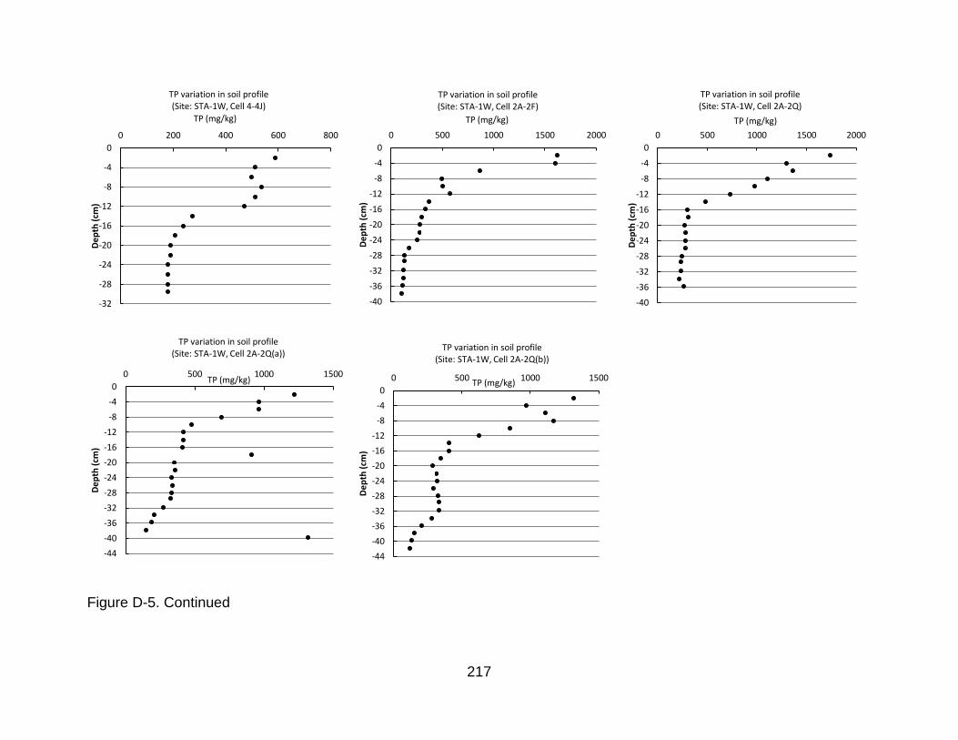
217
Figure D-5. Continued
-32
-28
-24
-20
-16
-12
-8
-4
0
0 200 400 600 800
De
pth
(cm
)
TP (mg/kg)
TP variation in soil profile (Site: STA-1W, Cell 4-4J)
-40
-36
-32
-28
-24
-20
-16
-12
-8
-4
0
0 500 1000 1500 2000
De
pth
(cm
)
TP (mg/kg)
TP variation in soil profile (Site: STA-1W, Cell 2A-2F)
-40
-36
-32
-28
-24
-20
-16
-12
-8
-4
0
0 500 1000 1500 2000
De
pth
(cm
)
TP (mg/kg)
TP variation in soil profile (Site: STA-1W, Cell 2A-2Q)
-44
-40
-36
-32
-28
-24
-20
-16
-12
-8
-4
0
0 500 1000 1500
De
pth
(cm
)
TP (mg/kg)
TP variation in soil profile (Site: STA-1W, Cell 2A-2Q(a))
-44
-40
-36
-32
-28
-24
-20
-16
-12
-8
-4
0
0 500 1000 1500
De
pth
(cm
)
TP (mg/kg)
TP variation in soil profile (Site: STA-1W, Cell 2A-2Q(b))

218
Figure D-6. Bulk density profile in each soil core collected from STA-2.
-40
-36
-32
-28
-24
-20
-16
-12
-8
-4
0
0.05 0.10 0.15 0.20 0.25
Dep
th (
cm)
Bulk density (g/cm3)
Bulk density variation in soil profile (Site: STA-2, Cell A-103)
-32
-28
-24
-20
-16
-12
-8
-4
0
0.05 0.10 0.15 0.20 0.25
Dep
th (
cm)
Bulk density (g/cm3)
Bulk density variation in soil profile (Site: STA-2, Cell A-103(a))
-44
-40
-36
-32
-28
-24
-20
-16
-12
-8
-4
0
0.05 0.10 0.15 0.20 0.25
Dep
th (
cm)
Bulk density (g/cm3) Bulk density variation in soil profile
(Site: STA-2, Cell A-103(b))
-36
-32
-28
-24
-20
-16
-12
-8
-4
0
0.05 0.10 0.15 0.20 0.25 0.30
Dep
th (
cm)
Bulk density (g/cm3) Bulk density variation in soil profile
(Site: STA-2, Cell A-51)
-48-44-40-36-32-28-24-20-16-12
-8-40
0.05 0.10 0.15 0.20 0.25D
epth
(cm
) Bulk density (g/cm3)
Bulk density variation in soil profile (Site: STA-2, Cell A-138)
-36
-32
-28
-24
-20
-16
-12
-8
-4
0
0.05 0.15 0.25 0.35
Dep
th (
cm)
Bulk density (g/cm3) Bulk density variation in soil profile
(Site: STA-2, Cell A-172)

219
Figure D-6. Continued
-36
-32
-28
-24
-20
-16
-12
-8
-4
0
0.05 0.15 0.25 0.35 0.45
Dep
th (
cm)
Bulk density (g/cm3) Bulk density variation in soil profile
(Site: STA-2, Cell C-75)
-36
-32
-28
-24
-20
-16
-12
-8
-4
0
0.05 0.15 0.25 0.35
Dep
th (
cm)
Bulk density (g/cm3)
Bulk density variation in soil profile (Site: STA-2, Cell C-75(a))
-20
-16
-12
-8
-4
0
0.05 0.15 0.25 0.35 0.45
Dep
th (
cm)
Bulk density (g/cm3)
Bulk density variation in soil profile (Site: STA-2, Cell C-75(b))
-28
-24
-20
-16
-12
-8
-4
0
0.05 0.25 0.45 0.65 0.85
Dep
th (
cm)
Bulk density (g/cm3) Bulk density variation in soil profile
(Site: STA-2, Cell C-21)
-40
-36
-32
-28
-24
-20
-16
-12
-8
-4
0
0.05 0.15 0.25 0.35 0.45
Dep
th (
cm)
Bulk density (g/cm3) Bulk density variation in soil profile
(Site: STA-2, Cell C-129)
-32
-28
-24
-20
-16
-12
-8
-4
0
0.05 0.55 1.05 1.55
Dep
th (
cm)
Bulk density (g/cm3)
Bulk density variation in soil profile (Site: STA-2, Cell C-165)

220
Figure D-6. Continued
-36
-32
-28
-24
-20
-16
-12
-8
-4
0
0.05 0.55 1.05 1.55
Dep
th (
cm)
Bulk density (g/cm3) Bulk density variation in soil profile
(Site: STA-2, Cell C-201)
-36
-32
-28
-24
-20
-16
-12
-8
-4
0
0.05 0.55 1.05 1.55
Dep
th (
cm)
Bulk density (g/cm3) Bulk density variation in soil profile
(Site: STA-2, Cell B-26)
-48-44-40-36-32-28-24-20-16-12
-8-40
0.05 0.10 0.15 0.20 0.25 0.30
Dep
th (
cm)
Bulk density (g/cm3) Bulk density variation in soil profile
(Site: STA-2, Cell B-81)
-28
-24
-20
-16
-12
-8
-4
0
0.05 0.15 0.25 0.35 0.45
Dep
th (
cm)
Bulk density (g/cm3) Bulk density variation in soil profile
(Site: STA-2, Cell B-98)
-48-44-40-36-32-28-24-20-16-12
-8-40
0.05 0.10 0.15 0.20 0.25 0.30
Dep
th (
cm)
Bulk density (g/cm3) Bulk density variation in soil profile
(Site: STA-2, Cell B-98(a))
-44-40-36-32-28-24-20-16-12
-8-40
0.05 0.10 0.15 0.20 0.25 0.30
Dep
th (
cm)
Bulk density (g/cm3) Bulk density variation in soil profile
(Site: STA-2, Cell B-98(b))

221
Figure D-6. Continued
-48
-44
-40
-36
-32
-28
-24
-20
-16
-12
-8
-4
0
0.05 0.10 0.15 0.20 0.25 0.30
Dep
th (
cm)
Bulk density (g/cm3) Bulk density variation in soil profile
(Site: STA-2, Cell B-117)
-44
-40
-36
-32
-28
-24
-20
-16
-12
-8
-4
0
0.05 0.10 0.15 0.20 0.25 0.30
Dep
th (
cm)
Bulk density (g/cm3) Bulk density variation in soil profile
(Site: STA-2, Cell B-151)
-44
-40
-36
-32
-28
-24
-20
-16
-12
-8
-4
0
0.05 0.10 0.15 0.20 0.25 0.30
Dep
th (
cm)
Bulk density (g/cm3) Bulk density variation in soil profile
(Site: STA-2, Cell B-187)
-48
-44
-40
-36
-32
-28
-24
-20
-16
-12
-8
-4
0
0.05 0.15 0.25 0.35
Dep
th (
cm)
Bulk density (g/cm3) Bulk density variation in soil profile
(Site: STA-2, Cell B-31)
-48
-44
-40
-36
-32
-28
-24
-20
-16
-12
-8
-4
0
0.05 0.15 0.25 0.35
Dep
th (
cm)
Bulk density (g/cm3) Bulk density variation in soil profile
(Site: STA-2, Cell B-31(a))
-20
-16
-12
-8
-4
0
0.05 0.25 0.45 0.65 0.85 1.05
Dep
th (
cm)
Bulk density (g/cm3)
Bulk density variation in soil profile (Site: STA-2, Cell D-111)

222
Figure D-6. Continued
-40
-36
-32
-28
-24
-20
-16
-12
-8
-4
0
0.05 0.15 0.25 0.35 0.45 0.55
Dep
th (
cm)
Bulk density (g/cm3) Bulk density variation in soil profile
(Site: STA-2, Cell D-124)
-32
-28
-24
-20
-16
-12
-8
-4
0
0.05 0.25 0.45 0.65
Dep
th (
cm)
Bulk density (g/cm3) Bulk density variation in soil profile
(Site: STA-2, Cell D-124(a))
-44
-40
-36
-32
-28
-24
-20
-16
-12
-8
-4
0
0.05 0.15 0.25 0.35 0.45 0.55
Dep
th (
cm)
Bulk density (g/cm3)
Bulk density variation in soil profile (Site: STA-2, Cell D-124(b))
-28
-24
-20
-16
-12
-8
-4
0
0.05 0.25 0.45 0.65
Dep
th (
cm)
Bulk density (g/cm3)
Bulk density variation in soil profile (Site: STA-2, Cell D-139)
-40
-36
-32
-28
-24
-20
-16
-12
-8
-4
0
0.05 0.15 0.25 0.35 0.45 0.55
Dep
th (
cm)
Bulk density (g/cm3) Bulk density variation in soil profile
(Site: STA-2, Cell D-129)

223
Figure D-7. Total phosphorus profile in each soil core collected from STA-2.
-40
-36
-32
-28
-24
-20
-16
-12
-8
-4
0
0 500 1000 1500 2000 2500
Dep
th (
cm)
TP (mg/kg)
TP variation in soil profile (Site: STA-2, Cell A-103)
-32
-28
-24
-20
-16
-12
-8
-4
0
0 200 400 600 800 1000
Dep
th (
cm)
TP (mg/kg) TP variation in soil profile (Site: STA-2, Cell A-103(a))
-44
-40
-36
-32
-28
-24
-20
-16
-12
-8
-4
0
0 500 1000 1500 2000
Dep
th (
cm)
TP (mg/kg)
TP variation in soil profile (Site: STA-2, Cell A-103(b))
-36
-32
-28
-24
-20
-16
-12
-8
-4
0
0 500 1000 1500 2000
Dep
th (
cm)
TP (mg/kg)
TP variation in soil profile (Site: STA-2, Cell A-51)
-36
-32
-28
-24
-20
-16
-12
-8
-4
0
0 500 1000 1500D
epth
(cm
)
TP (mg/kg) TP variation in soil profile (Site: STA-2, Cell A-172)
-44
-40
-36
-32
-28
-24
-20
-16
-12
-8
-4
0
0 500 1000 1500
Dep
th (
cm)
TP (mg/kg) TP variation in soil profile (Site: STA-2, Cell A-138)

224
Figure D-7. Continued
-28
-24
-20
-16
-12
-8
-4
0
0 200 400 600 800
Dep
th (
cm)
TP (mg/kg)
TP variation in soil profile (Site: STA-2, Cell C-21)
-40
-36
-32
-28
-24
-20
-16
-12
-8
-4
0
0 500 1000 1500
Dep
th (
cm)
TP (mg/kg)
TP variation in soil profile (Site: STA-2, Cell C-129)
-32
-28
-24
-20
-16
-12
-8
-4
0
0 200 400 600 800
Dep
th (
cm)
TP (mg/kg) TP variation in soil profile (Site: STA-2, Cell C-165)
-36
-32
-28
-24
-20
-16
-12
-8
-4
0
0 500 1000 1500
Dep
th (
cm)
TP (mg/kg)
TP variation in soil profile (Site: STA-2, Cell C-75)
-36
-32
-28
-24
-20
-16
-12
-8
-4
0
0 500 1000 1500
Dep
th (
cm)
TP (mg/kg)
TP variation in soil profile (Site: STA-2, Cell C-75(a))
-20
-16
-12
-8
-4
0
0 500 1000
Dep
th (
cm)
TP (mg/kg)
TP variation in soil profile (Site: STA-2, Cell C-75(b))

225
Figure D-7. Continued
-36
-32
-28
-24
-20
-16
-12
-8
-4
0
0 200 400 600 800 1000
Dep
th (
cm)
TP (mg/kg) TP variation in soil profile (Site: STA-2, Cell C-201)
-36
-32
-28
-24
-20
-16
-12
-8
-4
0
0 200 400 600 800 1000
Dep
th (
cm)
TP (mg/kg)
TP variation in soil profile (Site: STA-2, Cell B-26)
-44
-40
-36
-32
-28
-24
-20
-16
-12
-8
-4
0
0 500 1000 1500 2000
Dep
th (
cm)
TP (mg/kg)
TP variation in soil profile (Site: STA-2, Cell B-81)
-28
-24
-20
-16
-12
-8
-4
0
0 500 1000 1500
Dep
th (
cm)
TP (mg/kg)
TP variation in soil profile (Site: STA-2, Cell B-98)
-44
-40
-36
-32
-28
-24
-20
-16
-12
-8
-4
0
0 500 1000 1500 2000D
epth
(cm
) TP (mg/kg)
TP variation in soil profile (Site: STA-2, Cell B-98(a))
-44
-40
-36
-32
-28
-24
-20
-16
-12
-8
-4
0
0 500 1000 1500 2000
Dep
th (
cm)
TP (mg/kg)
TP variation in soil profile (Site: STA-2, Cell B-98(b))

226
Figure D-7. Continued
-48-44-40-36-32-28-24-20-16-12
-8-40
0 200 400 600 800 1000 1200
Dep
th (
cm)
TP (mg/kg)
TP variation in soil profile (Site: STA-2, Cell B-117)
-44
-40
-36
-32
-28
-24
-20
-16
-12
-8
-4
0
0 500 1000
Dep
th (
cm)
TP (mg/kg)
TP variation in soil profile (Site: STA-2, Cell B-151)
-44
-40
-36
-32
-28
-24
-20
-16
-12
-8
-4
0
0 500 1000 1500
Dep
th (
cm)
TP (mg/kg)
TP variation in soil profile (Site: STA-2, Cell B-187)
-48
-44
-40
-36
-32
-28
-24
-20
-16
-12
-8
-4
0
0 500 1000 1500 2000
Dep
th (
cm)
TP (mg/kg)
TP variation in soil profile (Site: STA-2, Cell B-31)
-48
-44
-40
-36
-32
-28
-24
-20
-16
-12
-8
-4
0
0 500 1000 1500 2000
Dep
th (
cm)
TP (mg/kg) TP variation in soil profile (Site: STA-2, Cell B-31(a))
-20
-16
-12
-8
-4
0
0 500 1000 1500
Dep
th (
cm)
TP (mg/kg) TP variation in soil profile (Site: STA-2, Cell D-111)

227
Figure D-7. Continued
-40
-36
-32
-28
-24
-20
-16
-12
-8
-4
0
0 200 400 600 800 1000
Dep
th (
cm)
TP (mg/kg)
TP variation in soil profile (Site: STA-2, Cell D-124)
-32
-28
-24
-20
-16
-12
-8
-4
0
0 200 400 600 800 1000
Dep
th (
cm)
TP (mg/kg)
TP variation in soil profile (Site: STA-2, Cell D-124(a))
-44
-40
-36
-32
-28
-24
-20
-16
-12
-8
-4
0
0 500 1000 1500
Dep
th (
cm)
TP (mg/kg)
TP variation in soil profile (Site: STA-2, Cell D-124(b))
-28
-24
-20
-16
-12
-8
-4
0
0 200 400 600 800
Dep
th (
cm)
TP (mg/kg)
TP variation in soil profile (Site: STA-2, Cell D-139)
-40
-36
-32
-28
-24
-20
-16
-12
-8
-4
0
0 200 400 600 800
Dep
th (
cm)
TP (mg/kg) TP variation in soil profile (Site: STA-2, Cell D-129)

228
EAV cell EAV cell EAV cell
EAV cell EAV cell EAV cell Figure D-8. Bulk density profile in each soil core collected from STA-3/4.
-40
-36
-32
-28
-24
-20
-16
-12
-8
-4
0
0.05 0.25 0.45 0.65 0.85
Dep
th (
cm)
Bulk density (g/cm3)
Bulk density variation in soil profile (Site: STA-3/4, Cell 2A-1)
-28
-24
-20
-16
-12
-8
-4
0
0.05 0.25 0.45 0.65 0.85 1.05
Dep
th (
cm)
Bulk density (g/cm3)
Bulk density variation in soil profile (Site: STA-3/4, Cell 2A-5)
-16
-12
-8
-4
0
0.05 0.25 0.45 0.65
Dep
th (
cm)
Bulk density (g/cm3)
Bulk density variation in soil profile (Site: STA-3/4, Cell 2A-12)
-28
-24
-20
-16
-12
-8
-4
0
0.05 0.25 0.45 0.65 0.85 1.05
Dep
th (
cm)
Bulk density (g/cm3)
Bulk density variation in soil profile (Site: STA-3/4, Cell 2A-16)
-20
-16
-12
-8
-4
0
0.05 0.15 0.25 0.35 0.45
Dep
th (
cm)
Bulk density (g/cm3) Bulk density variation in soil profile
(Site: STA-3/4, Cell 2A-38)
-16
-12
-8
-4
0
0.05 0.15 0.25 0.35 0.45
Dep
th (
cm)
Bulk density (g/cm3)
Bulk density variation in soil profile (Site: STA-3/4, Cell 2A-42)

229
EAV cell EAV cell EAV cell
EAV cell EAV cell EAV cell Figure D-8. Continued
-12
-8
-4
0
0.05 0.25 0.45 0.65 0.85
Dep
th (
cm)
Bulk density (g/cm3)
Bulk density variation in soil profile (Site: STA-3/4, Cell 2A-24)
-16
-12
-8
-4
0
0.05 0.15 0.25 0.35 0.45 0.55
Dep
th (
cm)
Bulk density (g/cm3)
Bulk density variation in soil profile (Site: STA-3/4, Cell 2A-24(a))
-12
-8
-4
0
0.05 0.15 0.25 0.35 0.45 0.55
Dep
th (
cm)
Bulk density (g/cm3)
Bulk density variation in soil profile (Site: STA-3/4, Cell 2A-24(b))
-8
-4
0
0.05 0.25 0.45 0.65
Dep
th (
cm)
Bulk density (g/cm3)
Bulk density variation in soil profile (Site: STA-3/4, Cell 2A-28)
-12
-8
-4
0
0.05 0.15 0.25 0.35 0.45 0.55
Dep
th (
cm)
Bulk density (g/cm3)
Bulk density variation in soil profile (Site: STA-3/4, Cell 2A-28(a))
-12
-8
-4
0
0.05 0.15 0.25 0.35 0.45 0.55
Dep
th (
cm)
Bulk density (g/cm3)
Bulk density variation in soil profile (Site: STA-3/4, Cell 2A-28(b))

230
EAV cell EAV cell EAV cell
SAV cell SAV cell SAV cell
Figure D-8. Continued
-32
-28
-24
-20
-16
-12
-8
-4
0
0.00 0.20 0.40 0.60 0.80
Dep
th (
cm)
Bulk density (g/cm3)
Bulk density variation in soil profile (Site: STA-3/4, Cell 2A-57)
-32
-28
-24
-20
-16
-12
-8
-4
0
0.05 0.15 0.25 0.35 0.45
Dep
th (
cm)
Bulk density (g/cm3)
Bulk density variation in soil profile (Site: STA-3/4, Cell 2A-53)
-8
-4
0
0.05 0.07 0.09 0.11 0.13 0.15
Dep
th (
cm)
Bulk density (g/cm3)
Bulk density variation in soil profile (Site: STA-3/4, Cell 2A-53(a))
-12
-8
-4
0
0.05 0.25 0.45 0.65
Dep
th (
cm)
Bulk density (g/cm3)
Bulk density variation in soil profile (Site: STA-3/4, Cell 2B-17)
-16
-12
-8
-4
0
0.05 0.25 0.45 0.65 0.85
Dep
th (
cm)
Bulk density (g/cm3)
Bulk density variation in soil profile (Site: STA-3/4, Cell 2B-17(a))
-16
-12
-8
-4
0
0.05 0.25 0.45 0.65 0.85
Dep
th (
cm)
Bulk density (g/cm3)
Bulk density variation in soil profile (Site: STA-3/4, Cell 2B-17(b))

231
SAV cell SAV cell SAV cell
SAV cell SAV cell SAV cell Figure D-8. Continued
-16
-12
-8
-4
0
0.05 0.25 0.45 0.65 0.85
Dep
th (
cm)
Bulk density (g/cm3)
Bulk density variation in soil profile (Site: STA-3/4, Cell 2B-3)
-24
-20
-16
-12
-8
-4
0
0.05 0.15 0.25 0.35 0.45 0.55
Dep
th (
cm)
Bulk density (g/cm3)
Bulk density variation in soil profile (Site: STA-3/4, Cell 2B-21)
-32
-28
-24
-20
-16
-12
-8
-4
0
0.05 0.25 0.45 0.65
Dep
th (
cm)
Bulk density (g/cm3)
Bulk density variation in soil profile (Site: STA-3/4, Cell 2B-24)
-16
-12
-8
-4
0
0.05 0.25 0.45 0.65
Dep
th (
cm)
Bulk density (g/cm3)
Bulk density variation in soil profile (Site: STA-3/4, Cell 2B-28)
-16
-12
-8
-4
0
0.05 0.25 0.45 0.65
Dep
th (
cm)
Bulk density (g/cm3)
Bulk density variation in soil profile (Site: STA-3/4, Cell 2B-40)
-16
-12
-8
-4
0
0.05 0.15 0.25 0.35 0.45 0.55
Dep
th (
cm)
Bulk density (g/cm3)
Bulk density variation in soil profile (Site: STA-3/4, Cell 2B-55)

232
SAV cell SAV cell SAV cell
SAV cell SAV cell EAV cell Figure D-8. Continued
-16
-12
-8
-4
0
0.05 0.25 0.45 0.65
Dep
th (
cm)
Bulk density (g/cm3)
Bulk density variation in soil profile (Site: STA-3/4, Cell 2B-44)
-24
-20
-16
-12
-8
-4
0
0.05 0.25 0.45 0.65
Dep
th (
cm)
Bulk density (g/cm3)
Bulk density variation in soil profile (Site: STA-3/4, Cell 2B-44(a))
-24
-20
-16
-12
-8
-4
0
0.05 0.15 0.25 0.35 0.45 0.55
Dep
th (
cm)
Bulk density (g/cm3)
Bulk density variation in soil profile (Site: STA-3/4, Cell 2B-44(b))
-16
-12
-8
-4
0
0.05 0.25 0.45 0.65
Dep
th (
cm)
Bulk density (g/cm3)
Bulk density variation in soil profile (Site: STA-3/4, Cell 2B-59)
-16
-12
-8
-4
0
0.05 0.25 0.45 0.65
Dep
th (
cm)
Bulk density (g/cm3)
Bulk density variation in soil profile (Site: STA-3/4, Cell 2B-13)
-20
-16
-12
-8
-4
0
0.05 0.25 0.45 0.65 0.85
Dep
th (
cm)
Bulk density (g/cm3)
Bulk density variation in soil profile (Site: STA-3/4, Cell 1A-3)

233
EAV cell EAV cell EAV cell
EAV cell EAV cell EAV cell Figure D-8. Continued
-24
-20
-16
-12
-8
-4
0
0.05 0.25 0.45 0.65
Dep
th (
cm)
Bulk density (g/cm3)
Bulk density variation in soil profile (Site: STA-3/4, Cell 1A-32)
-24
-20
-16
-12
-8
-4
0
0.05 0.15 0.25 0.35 0.45 0.55
Dep
th (
cm)
Bulk density (g/cm3)
Bulk density variation in soil profile (Site: STA-3/4, Cell 1A-32(a))
-28
-24
-20
-16
-12
-8
-4
0
0.05 0.25 0.45 0.65 0.85
Dep
th (
cm)
Bulk density (g/cm3)
Bulk density variation in soil profile (Site: STA-3/4, Cell 1A-32(b))
-20
-16
-12
-8
-4
0
0.05 0.55 1.05 1.55
Dep
th (
cm)
Bulk density (g/cm3)
Bulk density variation in soil profile (Site: STA-3/4, Cell 1A-7)
-24
-20
-16
-12
-8
-4
0
0.00 0.20 0.40 0.60
De
pth
(cm
)
Bulk density (g/cm3)
Bulk density variation in soil profile (Site: STA-3/4, Cell 1A-21)
-16
-12
-8
-4
0
0.05 0.25 0.45 0.65 0.85
Dep
th (
cm)
Bulk density (g/cm3)
Bulk density variation in soil profile (Site: STA-3/4, Cell 1A-36)

234
EAV cell EAV cell EAV cell
EAV cell EAV cell EAV cell
Figure D-8. Continued
-28
-24
-20
-16
-12
-8
-4
0
0.05 0.25 0.45 0.65 0.85
Dep
th (
cm)
Bulk density (g/cm3)
Bulk density variation in soil profile (Site: STA-3/4, Cell 1A-48)
-20
-16
-12
-8
-4
0
0.05 0.15 0.25 0.35 0.45 0.55
Dep
th (
cm)
Bulk density (g/cm3)
Bulk density variation in soil profile (Site: STA-3/4, Cell 1A-71)
-24
-20
-16
-12
-8
-4
0
0.05 0.10 0.15 0.20 0.25 0.30
Dep
th (
cm)
Bulk density (g/cm3)
Bulk density variation in soil profile (Site: STA-3/4, Cell 1A-56)
-20
-16
-12
-8
-4
0
0.05 0.25 0.45 0.65
Dep
th (
cm)
Bulk density (g/cm3)
Bulk density variation in soil profile (Site: STA-3/4, Cell 1A-52)
-16
-12
-8
-4
0
0.05 0.15 0.25 0.35 0.45 0.55D
epth
(cm
) Bulk density (g/cm3)
Bulk density variation in soil profile (Site: STA-3/4, Cell 1A-52(a))
-16
-12
-8
-4
0
0.05 0.15 0.25 0.35 0.45 0.55
Dep
th (
cm)
Bulk density (g/cm3)
Bulk density variation in soil profile (Site: STA-3/4, Cell 1A-52(b))

235
EAV cell EAV cell EAV cell
EAV cell EAV cell EAV cell
Figure D-8. Continued
-16
-12
-8
-4
0
0.05 0.25 0.45 0.65
Dep
th (
cm)
Bulk density (g/cm3)
Bulk density variation in soil profile (Site: STA-3/4, Cell 1A-74)
-20
-16
-12
-8
-4
0
0.05 0.55 1.05 1.55 2.05
Dep
th (
cm)
Bulk density (g/cm3)
Bulk density variation in soil profile (Site: STA-3/4, Cell 1B-4)
-16
-12
-8
-4
0
0.05 0.25 0.45 0.65
Dep
th (
cm)
Bulk density (g/cm3)
Bulk density variation in soil profile (Site: STA-3/4, Cell 1B-8)
-20
-16
-12
-8
-4
0
0.05 0.15 0.25 0.35 0.45
Dep
th (
cm)
Bulk density (g/cm3)
Bulk density variation in soil profile (Site: STA-3/4, Cell 1B-24)
-28
-24
-20
-16
-12
-8
-4
0
0.05 0.25 0.45 0.65 0.85D
epth
(cm
) Bulk density (g/cm3)
Bulk density variation in soil profile (Site: STA-3/4, Cell 1B-28)
-36
-32
-28
-24
-20
-16
-12
-8
-4
0
0.05 0.15 0.25 0.35 0.45
Dep
th (
cm)
Bulk density (g/cm3)
Bulk density variation in soil profile (Site: STA-3/4, Cell 1B-56)

236
EAV cell EAV cell EAV cell
EAV cell EAV cell EAV cell Figure D-8. Continued
-36
-32
-28
-24
-20
-16
-12
-8
-4
0
0.05 0.25 0.45 0.65 0.85
Dep
th (
cm)
Bulk density (g/cm3)
Bulk density variation in soil profile (Site: STA-3/4, Cell 1B-80)
-24
-20
-16
-12
-8
-4
0
0.05 0.10 0.15 0.20 0.25 0.30 0.35
Dep
th (
cm)
Bulk density (g/cm3)
Bulk density variation in soil profile (Site: STA-3/4, Cell 1B-87)
-28
-24
-20
-16
-12
-8
-4
0
0.05 0.15 0.25 0.35 0.45 0.55
Dep
th (
cm)
Bulk density (g/cm3)
Bulk density variation in soil profile (Site: STA-3/4, Cell 1B-84)
-12
-8
-4
0
0.05 0.10 0.15 0.20 0.25 0.30 0.35
Dep
th (
cm)
Bulk density (g/cm3)
Bulk density variation in soil profile (Site: STA-3/4, Cell 1B-52)
-24
-20
-16
-12
-8
-4
0
0.05 0.25 0.45 0.65 0.85
Dep
th (
cm)
Bulk density (g/cm3)
Bulk density variation in soil profile (Site: STA-3/4, Cell 1B-52(a))
-16
-12
-8
-4
0
0.05 0.15 0.25 0.35 0.45
Dep
th (
cm)
Bulk density (g/cm3)
Bulk density variation in soil profile (Site: STA-3/4, Cell 1B-52(b))

237
EAV cell EAV cell EAV cell
Figure D-8. Continued
-40
-36
-32
-28
-24
-20
-16
-12
-8
-4
0
0.05 0.25 0.45 0.65 0.85
Dep
th (
cm)
Bulk density (g/cm3)
Bulk density variation in soil profile (Site: STA-3/4, Cell 1B-60)
-44
-40
-36
-32
-28
-24
-20
-16
-12
-8
-4
0
0.00 0.20 0.40 0.60 0.80
Dep
th (
cm)
Bulk density (g/cm3)
Bulk density variation in soil profile (Site: STA-3/4, Cell 1B-60(a))
-36
-32
-28
-24
-20
-16
-12
-8
-4
0
0.05 0.15 0.25 0.35 0.45 0.55 0.65
Dep
th (
cm)
Bulk density (g/cm3)
Bulk density variation in soil profile (Site: STA-3/4, Cell 1B-60(b))

238
EAV cell EAV cell EAV cell
EAV cell EAV cell EAV cell Figure D-9. Total phosphorus profile in each soil core collected from STA-3/4.
-40
-36
-32
-28
-24
-20
-16
-12
-8
-4
0
0 200 400 600 800 1000 1200
Dep
th (
cm)
TP (mg/kg)
TP variation in soil profile (Site: STA-3/4, Cell 2A-1)
-28
-24
-20
-16
-12
-8
-4
0
0 500 1000 1500
Dep
th (
cm)
TP (mg/kg)
TP variation in soil profile (Site: STA-3/4, Cell 2A-5)
-16
-12
-8
-4
0
0 200 400 600 800 1000
Dep
th (
cm)
TP (mg/kg)
TP variation in soil profile (Site: STA-3/4, Cell 2A-12)
-28
-24
-20
-16
-12
-8
-4
0
0 500 1000 1500 2000
Dep
th (
cm)
TP (mg/kg)
TP variation in soil profile (Site: STA-3/4, Cell 2A-16)
-20
-16
-12
-8
-4
0
0 500 1000 1500D
epth
(cm
) TP (mg/kg)
TP variation in soil profile (Site: STA-3/4, Cell 2A-38)
-16
-12
-8
-4
0
0 500 1000 1500
Dep
th (
cm)
TP (mg/kg)
TP variation in soil profile (Site: STA-3/4, Cell 2A-42)

239
EAV cell EAV cell EAV cell
EAV cell EAV cell EAV cell Figure D-9. Continued
-12
-8
-4
0
0 200 400 600 800
Dep
th (
cm)
TP (mg/kg)
TP variation in soil profile (Site: STA-3/4, Cell 2A-24)
-16
-12
-8
-4
0
0 200 400 600 800 1000 1200
Dep
th (
cm)
TP (mg/kg)
TP variation in soil profile (Site: STA-3/4, Cell 2A-24(a))
-12
-8
-4
0
0 200 400 600 800 1000 1200
Dep
th (
cm)
TP (mg/kg)
TP variation in soil profile (Site: STA-3/4, Cell 2A-24(b))
-8
-4
0
0 200 400 600 800
Dep
th (
cm)
TP (mg/kg)
TP variation in soil profile (Site: STA-3/4, Cell 2A-28)
-12
-8
-4
0
0 200 400 600 800 1000
Dep
th (
cm)
TP (mg/kg)
TP variation in soil profile (Site: STA-3/4, Cell 2A-28(a))
-12
-8
-4
0
0 200 400 600 800
Dep
th (
cm)
TP (mg/kg)
TP variation in soil profile (Site: STA-3/4, Cell 2A-28(b))

240
EAV cell EAV cell EAV cell
SAV cell SAV cell SAV cell Figure D-9. Continued
-32
-28
-24
-20
-16
-12
-8
-4
0
0 500 1000 1500
Dep
th (
cm)
TP (mg/kg)
TP variation in soil profile (Site: STA-3/4, Cell 2A-53)
-8
-4
0
0 200 400 600 800 1000 1200
Dep
th (
cm)
TP (mg/kg)
TP variation in soil profile (Site: STA-3/4, Cell 2A-53(a))
-32
-28
-24
-20
-16
-12
-8
-4
0
0 500 1000 1500 2000
Dep
th (
cm)
TP (mg/kg)
TP variation in soil profile (Site: STA-3/4, Cell 2A-57)
-16
-12
-8
-4
0
0 100 200 300 400 500 600
Dep
th (
cm)
TP (mg/kg)
TP variation in soil profile (Site: STA-3/4, Cell 2B-3)
-24
-20
-16
-12
-8
-4
0
0 500 1000 1500 2000
Dep
th (
cm)
TP (mg/kg)
TP variation in soil profile (Site: STA-3/4, Cell 2B-21)
-32
-28
-24
-20
-16
-12
-8
-4
0
0 200 400 600 800
Dep
th (
cm)
TP (mg/kg)
TP variation in soil profile (Site: STA-3/4, Cell 2B-24)

241
SAV cell SAV cell SAV cell
SAV cell SAV cell SAV cell Figure D-9. Continued
-12
-8
-4
0
0 200 400 600 800
Dep
th (
cm)
TP (mg/kg)
TP variation in soil profile (Site: STA-3/4, Cell 2B-17)
-16
-12
-8
-4
0
0 200 400 600 800
Dep
th (
cm)
TP (mg/kg)
TP variation in soil profile (Site: STA-3/4, Cell 2B-17(a))
-16
-12
-8
-4
0
0 200 400 600 800 1000
Dep
th (
cm)
TP (mg/kg)
TP variation in soil profile (Site: STA-3/4, Cell 2B-17(b))
-16
-12
-8
-4
0
0 200 400 600 800 1000
Dep
th (
cm)
TP (mg/kg)
TP variation in soil profile (Site: STA-3/4, Cell 2B-28)
-16
-12
-8
-4
0
0 200 400 600 800
Dep
th (
cm)
TP (mg/kg)
TP variation in soil profile (Site: STA-3/4, Cell 2B-40)
-16
-12
-8
-4
0
0 200 400 600 800 1000
Dep
th (
cm)
TP (mg/kg)
TP variation in soil profile (Site: STA-3/4, Cell 2B-55)

242
SAV cell SAV cell SAV cell
SAV cell SAV cell EAV cell Figure D-9. Continued
-16
-12
-8
-4
0
0 200 400 600 800
Dep
th (
cm)
TP (mg/kg)
TP variation in soil profile (Site: STA-3/4, Cell 2B-44)
-24
-20
-16
-12
-8
-4
0
0 200 400 600 800 1000
Dep
th (
cm)
TP (mg/kg)
TP variation in soil profile (Site: STA-3/4, Cell 2B-44(a))
-24
-20
-16
-12
-8
-4
0
0 200 400 600 800 1000
Dep
th (
cm)
TP (mg/kg)
TP variation in soil profile (Site: STA-3/4, Cell 2B-44(b))
-16
-12
-8
-4
0
0 500 1000 1500
Dep
th (
cm)
TP (mg/kg)
TP variation in soil profile (Site: STA-3/4, Cell 2B-59)
-16
-12
-8
-4
0
0 200 400 600 800
Dep
th (
cm)
TP (mg/kg)
TP variation in soil profile (Site: STA-3/4, Cell 2B-13)
-20
-16
-12
-8
-4
0
0 500 1000 1500 2000
Dep
th (
cm)
TP (mg/kg)
TP variation in soil profile (Site: STA-3/4, Cell 1A-3)

243
EAV cell EAV cell EAV cell
EAV cell EAV cell EAV cell Figure D-9. Continued
-20
-16
-12
-8
-4
0
0 200 400 600 800 1000
Dep
th (
cm)
TP (mg/kg)
TP variation in soil profile (Site: STA-3/4, Cell 1A-7)
-24
-20
-16
-12
-8
-4
0
0 500 1000 1500 2000
Dep
th (
cm)
TP (mg/kg)
TP variation in soil profile (Site: STA-3/4, Cell 1A-21)
-16
-12
-8
-4
0
0 500 1000 1500
Dep
th (
cm)
TP (mg/kg)
TP variation in soil profile (Site: STA-3/4, Cell 1A-36)
-24
-20
-16
-12
-8
-4
0
0 200 400 600 800 1000
Dep
th (
cm)
TP (mg/kg)
TP variation in soil profile (Site: STA-3/4, Cell 1A-32)
-24
-20
-16
-12
-8
-4
0
0 200 400 600 800 1000 1200
Dep
th (
cm)
TP (mg/kg)
TP variation in soil profile (Site: STA-3/4, Cell 1A-32(a))
-28
-24
-20
-16
-12
-8
-4
0
0 500 1000 1500
Dep
th (
cm)
TP (mg/kg)
TP variation in soil profile (Site: STA-3/4, Cell 1A-32(b))

244
EAV cell EAV cell EAV cell
EAV cell EAV cell EAV cell Figure D-9. Continued
-28
-24
-20
-16
-12
-8
-4
0
0 500 1000 1500
Dep
th (
cm)
TP (mg/kg)
TP variation in soil profile (Site: STA-3/4, Cell 1A-48)
-24
-20
-16
-12
-8
-4
0
0 200 400 600 800 1000 1200
Dep
th (
cm)
TP (mg/kg)
TP variation in soil profile (Site: STA-3/4, Cell 1A-56)
-20
-16
-12
-8
-4
0
0 200 400 600 800 1000
Dep
th (
cm)
TP (mg/kg)
TP variation in soil profile (Site: STA-3/4, Cell 1A-71)
-20
-16
-12
-8
-4
0
0 200 400 600 800 1000
Dep
th (
cm)
TP (mg/kg)
TP variation in soil profile (Site: STA-3/4, Cell 1A-52)
-16
-12
-8
-4
0
0 200 400 600 800 1000
Dep
th (
cm)
TP (mg/kg)
TP variation in soil profile (Site: STA-3/4, Cell 1A-52(a))
-16
-12
-8
-4
0
0 200 400 600 800 1000
Dep
th (
cm)
TP (mg/kg)
TP variation in soil profile (Site: STA-3/4, Cell 1A-52(b))

245
EAV cell EAV cell EAV cell
EAV cell EAV cell EAV cell Figure D-9. Continued
-16
-12
-8
-4
0
0 500 1000 1500
Dep
th (
cm)
TP (mg/kg)
TP variation in soil profile (Site: STA-3/4, Cell 1A-74)
-20
-16
-12
-8
-4
0
0 200 400 600 800
Dep
th (
cm)
TP (mg/kg)
TP variation in soil profile (Site: STA-3/4, Cell 1B-4)
-16
-12
-8
-4
0
0 200 400 600 800 1000
Dep
th (
cm)
TP (mg/kg)
TP variation in soil profile (Site: STA-3/4, Cell 1B-8)
-20
-16
-12
-8
-4
0
0 500 1000 1500
Dep
th (
cm)
TP (mg/kg) TP variation in soil profile (Site: STA-3/4, Cell 1B-24)
-28
-24
-20
-16
-12
-8
-4
0
0 200 400 600 800D
epth
(cm
) TP (mg/kg)
TP variation in soil profile (Site: STA-3/4, Cell 1B-28)
-36
-32
-28
-24
-20
-16
-12
-8
-4
0
0 500 1000
Dep
th (
cm)
TP (mg/kg)
TP variation in soil profile (Site: STA-3/4, Cell 1B-56)

246
EAV cell EAV cell EAV cell
EAV cell EAV cell EAV cell Figure D-9. Continued
-36
-32
-28
-24
-20
-16
-12
-8
-4
0
0 200 400 600 800
Dep
th (
cm)
TP (mg/kg)
TP variation in soil profile (Site: STA-3/4, Cell 1B-80)
-28
-24
-20
-16
-12
-8
-4
0
0 200 400 600 800 1000
Dep
th (
cm)
TP (mg/kg)
TP variation in soil profile (Site: STA-3/4, Cell 1B-84)
-24
-20
-16
-12
-8
-4
0
0 200 400 600 800
Dep
th (
cm)
TP (mg/kg)
TP variation in soil profile (Site: STA-3/4, Cell 1B-87)
-12
-8
-4
0
0 500 1000 1500
Dep
th (
cm)
TP (mg/kg)
TP variation in soil profile (Site: STA-3/4, Cell 1B-52)
-24
-20
-16
-12
-8
-4
0
0 500 1000 1500D
epth
(cm
) TP (mg/kg)
TP variation in soil profile (Site: STA-3/4, Cell 1B-52(a))
-16
-12
-8
-4
0
0 500 1000 1500
Dep
th (
cm)
TP (mg/kg)
TP variation in soil profile (Site: STA-3/4, Cell 1B-52(b))

247
EAV cell EAV cell EAV cell Figure D-9. Continued
-40
-36
-32
-28
-24
-20
-16
-12
-8
-4
0
0 500 1000 1500
Dep
th (
cm)
TP (mg/kg)
TP variation in soil profile (Site: STA-3/4, Cell 1B-60)
-44
-40
-36
-32
-28
-24
-20
-16
-12
-8
-4
0
0 500 1000 1500
Dep
th (
cm)
TP (mg/kg)
TP variation in soil profile (Site: STA-3/4, Cell 1B-60(a))
-36
-32
-28
-24
-20
-16
-12
-8
-4
0
0 500 1000 1500
Dep
th (
cm)
TP (mg/kg)
TP variation in soil profile (Site: STA-3/4, Cell 1B-60(b))

248
APPENDIX E ADDITIONAL DATA AND INFORMATION PERTAINING TO CHAPTER 5
Table E-1. STA-1W and STA-2 soil core collection sites by vegetation type and cell. A total 44 soil cores were collected from these locations.
Soil core sampling locations
EAV SAV EAV conversion
STA- 1W Cell 5A Cell 5B Cell 3
5A112 5A150 5B108 5B202 3I 3P
5A112(a) 5A74 5B125 5B83 3I(a) 3B
5A112(b) -- 5B125(a) 5B162 3I(b) --
-- -- 5B125(b) -- -- --
EAV SAV
STA-2 Cell 1 Cell 2 Cell 3 Cell 4 -- --
A103 B117 C129 D111 -- --
A103(a) B151 C165 D124 -- --
A103(b) B187 C201 D124(a) -- --
A138 B26 C21 D124(b) -- --
A172 B81 C75 D129 -- --
A51 B98 C75(a) D139 -- --
-- B98(a) C75(b) -- -- --
-- B98(b) -- -- -- --

249
Table E-2. Mean depth of RAS at STA-1W sampling sites used for separating RAS from pre-STA soil.
STA-1W
EAV SAV EAV conversion
Cell 5A Cell 5B Cell 3
Site Depth (cm) Site Depth (cm)
Site Depth (cm)
5A112 8 5B108 8 3I 12
5A112(a) 8 5B125 8 3I(a) 10
5A112(b) 8 5B125(a) 8 3I(b) 10
5A150 10 5B125(b) 12 3P 10
5A74 16 5B202 8 3B 12
-- -- 5B83 10 -- --
-- -- 5B162 12 -- --
Table E-3. Mean depth of RAS at STA-2 sampling sites used for separating RAS from
pre-STA soil.
STA-2
EAV SAV
Cell 1 Cell 2 Cell 3 Cell 4
Site Depth (cm)
Site Depth (cm)
Site Depth (cm)
Site Depth (cm)
A103 8 B117 10 C129 8 D111 6
A103(a)* 12 B151 12 C165 12 D124 8
A103(b)* 8 B187 14 C201 10 D124(a) 12
A138 10 B26 8 C21 8 D124(b) 12
A172 8 B81 12 C75 8 D129 12
A51 8 B98 8 C75(a) 12 D139 12
-- - B98(a) 8 C75(b) 4 -- -
-- - B98(b) 8 -- -- -- -

250
Table E-4. Depth of soil fraction, bulk density, total phosphorus concentration and TP storage for each soil fraction at sampling sites in STA-1W.
STA-1W Floc RAS Pre-STA soil
EAV Depth Bulk
density TP
Conc. TP
Storage Depth
Bulk density
TP Conc.
TP Storage
Depth Bulk
density TP
Conc. TP
Storage
cm g cm-3 mg Pkg-1 g P m-2 cm g cm-3 mg P kg-1 g P m-2 cm g cm-3 mg Pkg-1 g Pm-2
Cell-5A
5A-112 8 0.11 1219 11.2 8 0.29 461 10.5 15 0.35 369 19.5
5A-112(a) 5 0.12 1080 6.5 8 0.31 444 11.0 15 0.34 428 21.8
5A-112(b) 8 0.08 1340 8.8 8 0.29 827 19.0 15 0.39 443 25.6
5A-150 16 0.05 1339 10.9 10 0.32 245 7.9 15 0.23 182 6.4
5A-74 -- -- -- -- 16 0.37 684 40.5 15 0.34 497 25.3
SAV
Cell-3
3B 8 0.18 334 4.7 12 0.31 226 8.4 15 0.33 222 10.9
3I 8 0.08 1094 7.3 12 0.23 446 12.5 15 0.26 186 7.2
3I(a) 6 0.05 1460 4.3 10 0.17 1045 17.9 15 0.26 210 8.3
3I(b) 8 0.06 940 4.5 10 0.22 789 17.2 15 0.28 198 8.3
3P 14 0.09 660 8.3 10 0.21 384 8.1 15 0.29 202 8.9
Cell-5B
5B-108 6 0.21 1002 12.8 8 0.35 426 12.0 15 0.19 255 7.3
5B-125 5 0.14 1199 8.1 8 0.26 568 12.0 15 0.28 322 13.4
5B-125(a) 6 0.13 986 8.0 8 0.28 353 7.9 15 0.28 298 12.3
5B-125(b) 5 0.10 778 3.8 12 0.33 426 17.0 15 0.32 364 17.6
5B-162 8 0.17 1011 13.7 12 0.28 508 17.2 15 0.27 396 16.2
5B-202 4 0.20 798 6.5 8 0.31 552 13.9 15 0.28 326 13.5
5B-83 6 0.09 690 3.9 10 0.39 733 28.6 15 0.32 588 28.2
*For pre-STA soil, TP storages were calculated only for a 15-cm deep soil layer, assuming constant bulk density throughout the layer.

251
Table E-5. Depth of soil fraction, bulk density, total phosphorus concentration and TP storage for each soil fraction at sampling sites in STA-2.
STA-2 Floc RAS Pre-STA soil
EAV Depth Bulk
density TP
Conc. TP
Storage Depth
Bulk density
TP Conc.
TP Storage
Depth Bulk
density TP
Conc. TP
Storage*
cm g cm-3 mg Pkg-1 g P m-2 cm g cm-3 mg P kg-1 g P m-2 cm g cm-3 mg Pkg-1 g Pm-2
Cell 1
A103 10 0.08 1014 7.7 8 0.18 255 3.7 15 0.14 178 3.8
A103 (a) 10 0.08 1098 8.3 12 0.16 275 5.3 15 0.13 162 3.1
A103 (b) 12 0.07 1031 8.9 8 0.14 297 3.3 15 0.14 174 3.6
A138 8 0.07 760 4.2 10 0.21 276 5.7 15 0.11 172 2.9
A172 8 0.04 1009 3.1 8 0.31 302 7.5 15 0.12 186 3.3
A51 9 0.04 1444 5.3 8 0.17 636 8.5 15 0.17 192 5.0
Cell 2
B117 7 0.08 644 3.6 10 0.25 317 8.1 15 0.13 181 3.6
B151 5 0.02 1455 1.5 12 0.15 554 10.2 15 0.18 220 5.8
B187 12 0.03 1117 3.8 14 0.19 455 12.3 15 0.41 199 12.2
B26 4 0.02 798 0.6 8 0.38 482 14.7 15 0.39 330 19.2
B81 7 0.12 1293 10.7 12 0.27 380 12.5 15 0.15 170 3.8
B98 10 0.04 1361 5.0 8 0.26 395 8.2 15 0.11 249 4.1
B98(a) 6 0.07 1116 4.8 8 0.20 406 6.4 15 0.12 174 3.1
B98(b) 10 0.07 1218 8.1 8 0.21 340 5.8 15 0.09 176 2.3
For pre-STA soil fraction, mass P storages were calculated only for 15 cm depth, assuming constant bulk density for the entire 15 cm depth.

252
Table E-5 Continued
STA-2 Floc RAS Pre-STA soil
SAV Depth Bulk
density TP
Conc. TP
Storage Depth
Bulk density
TP Conc.
TP Storage
Depth Bulk
density TP
Conc. TP
Storage
cm g cm-3 mg Pkg-1 g P m-2 cm g cm-3 mg P kg-1 g P m-2 cm g cm-3 mg Pkg-1 g Pm-2
Cell 3
C129 8 0.12 523 5.2 8 0.25 370 7.5 15 0.26 280 10.7
C165 7 0.10 506 3.5 12 0.30 389 14.2 15 0.22 242 8.0
C201 11 0.12 362 4.9 10 0.32 513 16.4 15 0.39 236 13.8
C21 5 0.13 886 5.9 8 0.46 399 14.6 15 0.39 431 25.3
C75 10 0.12 1083 12.8 8 0.23 777 14.5 15 0.14 284 6.2
C75 (a) 10 0.13 1020 13.2 12 0.24 753 21.9 15 0.20 278 8.3
C75 (b) 7 0.10 979 7.0 4 0.27 525 5.7 15 0.18 297 8.0
Cell 4
D111 -- -- -- -- 6 0.25 967 14.6 15 0.25 294 10.8
D124 -- -- -- -- 8 0.18 751 10.6 15 0.35 75 3.9
D124 (a) -- -- -- -- 12 0.24 655 19.1 15 0.32 405 19.4
D124 (b) -- -- -- -- 12 0.29 585 20.5 15 0.26 363 14.2
D129 -- -- -- -- 12 0.31 610 22.8 15 0.39 414 24.0
D139 -- -- -- -- 12 0.34 607 25.1 15 0.38 534 30.3
*For pre-STA soil, TP storages were calculated only for a 15 cm deep soil layer, assuming constant bulk density throughout the layer.

253
Table E-6. Depth of soil fraction, bulk density, total nitrogen concentration and TN storage for each soil fraction at sampling sites in STA-1W.
STA-1W Floc RAS Pre-STA soil
EAV Depth Bulk
density TN
Conc. TN
Storage Depth
Bulk density
TN Conc.
TN Storage
Depth Bulk
density TN
Conc. TN*
Storage
cm g cm-3 g Nkg-1 kg N m-2 cm g cm-3 g Nkg-1 kg N m-2 cm g cm-3 g Nkg-1 kg N m-2
Cell-5A
5A-112 8 0.11 29.0 0.27 8.0 0.3 28.1 0.64 15 0.4 28.6 1.51
5A-112(a) 5 0.12 28.3 0.17 8.0 0.3 27.6 0.69 15 0.3 28.7 1.47
5A-112(b) 8 0.08 27.7 0.18 8.0 0.3 24.6 0.56 15 0.4 28.9 1.67
5A-150 16 0.05 33.9 0.28 10.0 0.3 35.6 1.15 15 0.2 38.8 1.36
5A-74 -- -- -- -- 16.0 0.4 28.6 1.69 15 0.3 34.0 1.73
SAV
Cell-3
3B 8 0.18 33.5 0.47 12.0 0.3 35.8 1.34 15 0.3 35.7 1.75
3I 8 0.08 33.2 0.22 12.0 0.2 31.4 0.88 15 0.3 32.3 1.25
3I(a) 6 0.05 32.6 0.10 10.0 0.2 48.9 0.84 15 0.3 31.8 1.25
3I(b) 8 0.06 34.2 0.16 10.0 0.2 33.5 0.73 15 0.3 33.0 1.37
3P 14 0.09 30.4 0.38 10.0 0.2 31.4 0.66 15 0.3 30.3 1.34
Cell-5B
5B-108 6 0.21 29.6 0.38 8.0 0.4 37.1 1.05 15 0.2 38.1 1.08
5B-125 5 0.14 23.9 0.16 8.0 0.3 28.9 0.61 15 0.3 32.5 1.36
5B-125(a) 6 0.13 24.9 0.20 8.0 0.3 30.3 0.68 15 0.3 31.4 1.30
5B-125(b) 5 0.10 25.5 0.12 12.0 0.3 29.8 1.19 15 0.3 31.8 1.54
5B-162 8 0.17 27.9 0.38 12.0 0.3 34.7 1.17 15 0.3 34.8 1.42
5B-202 4 0.20 30.2 0.25 8.0 0.3 33.2 0.83 15 0.3 32.6 1.35
5B-83 6 0.09 32.2 0.18 10.0 0.4 35.8 1.40 15 0.3 36.8 1.76
*For pre-STA soil, TN storages were calculated only for a 15-cm deep soil layer, assuming constant bulk density throughout the layer.

254
Table E-7. Depth of soil fraction, bulk density, total nitrogen concentration and TN storage for each soil fraction at sampling sites in STA-2.
STA-2 Floc RAS Pre-STA soil
EAV Dept
h Bulk
density TN
Conc. TN
Storage Depth
Bulk density
TN Conc.
TN Storage
Depth Bulk
density
TN Conc.
TN* Storage
cm g cm-3 g Nkg-1 kg N m-2 cm g cm-3 g Nkg-1 kg N m-2 cm g cm-3 g Nkg-1 kg N m-2
Cell 1
A103 10 0.08 25.9 0.20 8.0 0.2 29.2 0.43 15 0.1 26.7 0.56
A103 (a) 10 0.08 29.2 0.22 12.0 0.2 30.4 0.58 15 0.1 26.1 0.51
A103 (b) 12 0.07 27.3 0.24 8.0 0.1 31.8 0.36 15 0.1 28.3 0.58
A138 8 0.07 26.8 0.15 10.0 0.2 31.4 0.65 15 0.1 29.4 0.50
A172 8 0.04 28.6 0.09 8.0 0.3 31.8 0.79 15 0.1 29.9 0.54
A51 9 0.04 28.2 0.10 8.0 0.2 29.0 0.39 15 0.2 28.7 0.75
Cell 2
B117 7 0.08 30.3 0.17 10.0 0.3 30.1 0.76 15 0.1 26.1 0.52
B151 5 0.02 28.3 0.03 12.0 0.2 29.3 0.54 15 0.2 28.5 0.75
B187 12 0.03 26.9 0.09 14.0 0.2 30.9 0.83 15 0.4 26.8 1.63
B26 4 0.02 13.2 0.01 8.0 0.4 24.5 0.75 15 0.4 27.9 1.63
B81 7 0.12 24.3 0.20 12.0 0.3 29.9 0.98 15 0.1 27.9 0.62
B98 10 0.04 24.3 0.09 8.0 0.3 29.2 0.60 15 0.1 28.9 0.47
B98(a) 6 0.07 29.2 0.13 8.0 0.2 31.3 0.50 15 0.1 27.9 0.50
B98(b) 10 0.07 28.0 0.19 8.0 0.2 29.9 0.51 15 0.1 26.8 0.35
*For pre-STA soil, TN storages were calculated only for a 15-cm deep soil layer, assuming constant bulk density throughout the layer.

255
Table E-7 Continued
STA-2 Floc RAS Pre-STA soil
SAV Depth Bulk
density TN
Conc. TN
Storage Depth
Bulk density
TN Conc.
TN Storage
Depth Bulk
density TN
Conc. TN
Storage
cm g cm-3 g Nkg-1 kg N m-2 cm g cm-3 g Nkg-1 kg N m-2 cm g cm-3 g Nkg-1 kg N m-2
Cell 3
C129 8 0.12 10.1 0.10 8.0 0.3 22.0 0.45 15 0.3 28.7 1.10
C165 7 0.10 16.1 0.11 12.0 0.3 30.9 1.13 15 0.2 37.8 1.25
C201 11 0.12 11.9 0.16 10.0 0.3 32.2 1.03 15 0.4 19.0 1.11
C21 5 0.13 12.0 0.08 8.0 0.5 28.5 1.04 15 0.4 19.0 1.12
C75 10 0.12 11.9 0.14 8.0 0.2 16.2 0.30 15 0.1 32.6 0.71
C75 (a) 10 0.13 11.4 0.15 12.0 0.2 17.5 0.51 15 0.2 28.1 0.84
C75 (b) 7 0.10 13.2 0.09 4.0 0.3 23.5 0.26 15 0.2 31.1 0.84
Cell 4
D111 -- -- -- -- 6.0 0.3 25.5 0.38 15 0.2 34.9 1.29
D124 -- -- -- -- 8.0 0.2 30.7 0.43 15 0.3 30.5 1.59
D124 (a) -- -- -- -- 12.0 0.2 30.5 0.89 15 0.3 29.0 1.39
D124 (b) -- -- -- -- 12.0 0.3 30.2 1.06 15 0.3 30.3 1.19
D129 -- -- -- -- 12.0 0.3 27.4 1.03 15 0.4 30.9 1.79
D139 -- -- -- -- 12.0 0.3 28.0 1.16 15 0.4 32.2 1.82
For pre-STA soil fraction, mass N storages were calculated only for 15 cm depth, assuming constant bulk density for the entire 15 cm depth.
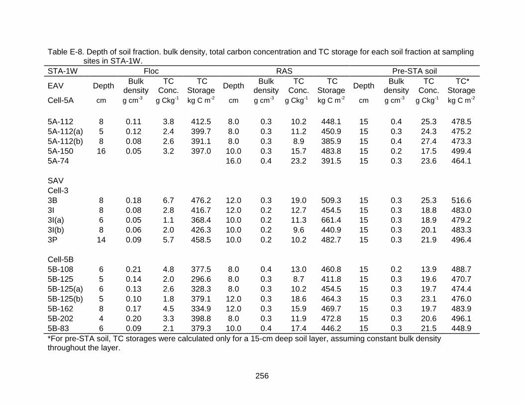
256
Table E-8. Depth of soil fraction. bulk density, total carbon concentration and TC storage for each soil fraction at sampling sites in STA-1W.
STA-1W Floc RAS Pre-STA soil
EAV Depth Bulk
density TC
Conc. TC
Storage Depth
Bulk density
TC Conc.
TC Storage
Depth Bulk
density TC
Conc. TC*
Storage
Cell-5A cm g cm-3 g Ckg-1 kg C m-2 cm g cm-3 g Ckg-1 kg C m-2 cm g cm-3 g Ckg-1 kg C m-2
5A-112 8 0.11 3.8 412.5 8.0 0.3 10.2 448.1 15 0.4 25.3 478.5
5A-112(a) 5 0.12 2.4 399.7 8.0 0.3 11.2 450.9 15 0.3 24.3 475.2
5A-112(b) 8 0.08 2.6 391.1 8.0 0.3 8.9 385.9 15 0.4 27.4 473.3
5A-150 16 0.05 3.2 397.0 10.0 0.3 15.7 483.8 15 0.2 17.5 499.4
5A-74 16.0 0.4 23.2 391.5 15 0.3 23.6 464.1
SAV
Cell-3
3B 8 0.18 6.7 476.2 12.0 0.3 19.0 509.3 15 0.3 25.3 516.6
3I 8 0.08 2.8 416.7 12.0 0.2 12.7 454.5 15 0.3 18.8 483.0
3I(a) 6 0.05 1.1 368.4 10.0 0.2 11.3 661.4 15 0.3 18.9 479.2
3I(b) 8 0.06 2.0 426.3 10.0 0.2 9.6 440.9 15 0.3 20.1 483.3
3P 14 0.09 5.7 458.5 10.0 0.2 10.2 482.7 15 0.3 21.9 496.4
Cell-5B
5B-108 6 0.21 4.8 377.5 8.0 0.4 13.0 460.8 15 0.2 13.9 488.7
5B-125 5 0.14 2.0 296.6 8.0 0.3 8.7 411.8 15 0.3 19.6 470.7
5B-125(a) 6 0.13 2.6 328.3 8.0 0.3 10.2 454.5 15 0.3 19.7 474.4
5B-125(b) 5 0.10 1.8 379.1 12.0 0.3 18.6 464.3 15 0.3 23.1 476.0
5B-162 8 0.17 4.5 334.9 12.0 0.3 15.9 469.7 15 0.3 19.7 483.9
5B-202 4 0.20 3.3 398.8 8.0 0.3 11.9 472.8 15 0.3 20.6 496.1
5B-83 6 0.09 2.1 379.3 10.0 0.4 17.4 446.2 15 0.3 21.5 448.9
*For pre-STA soil, TC storages were calculated only for a 15-cm deep soil layer, assuming constant bulk density throughout the layer.

257
Table E-9. Depth of soil fraction, bulk density, total carbon concentration and TC storage for each soil fraction at sampling sites in STA-2.
STA-2 Floc RAS Pre-STA soil
EAV Depth Bulk
density TC
Conc. TC
Storage Depth
Bulk density
TC Conc.
TC Storage
Depth Bulk
density TC
Conc. TC*
Storage
Cell1 cm g cm-3 g Ckg-1 kg C m-2 cm g cm-3 g Ckg-1 kg C m-2 cm g cm-3 g Ckg-1 kg C m-2
A103 10 0.08 2.6 342.8 8.0 0.2 6.5 445.8 15 0.1 9.5 453.6
A103 (a) 10 0.08 2.9 377.2 12.0 0.2 8.4 441.2 15 0.1 8.9 458.6
A103 (b) 12 0.07 3.0 354.0 8.0 0.1 4.9 436.4 15 0.1 9.6 469.2
A138 8 0.07 2.3 411.6 10.0 0.2 9.3 450.3 15 0.1 8.3 484.6
A172 8 0.04 1.2 379.6 8.0 0.3 11.0 442.8 15 0.1 8.5 473.4
A51 9 0.04 1.4 377.0 8.0 0.2 5.7 426.1 15 0.2 12.5 478.7
Cell 2
B117 7 0.08 2.4 429.8 10.0 0.3 11.6 457.1 15 0.1 9.6 481.4
B151 5 0.02 0.4 406.9 12.0 0.2 8.3 448.2 15 0.2 12.5 475.5
B187 12 0.03 1.4 401.6 14.0 0.2 12.3 457.1 15 0.4 29.1 476.4
B26 4 0.02 0.2 223.2 8.0 0.4 12.6 415.3 15 0.4 27.6 474.4
B81 7 0.12 2.9 345.9 12.0 0.3 15.0 456.8 15 0.1 11.0 494.0
B98 10 0.04 1.3 343.0 8.0 0.3 9.1 441.0 15 0.1 7.5 457.2
B98(a) 6 0.07 1.7 384.5 8.0 0.2 6.9 435.8 15 0.1 8.5 472.0
B98(b) 10 0.07 2.5 382.9 8.0 0.2 7.5 444.5 15 0.1 6.0 465.0
*For pre-STA soil, TC storages were calculated only for a 15-cm deep soil layer, assuming constant bulk density throughout the layer.

258
Table E-9 continued.
STA-2 Floc RAS Pre-STA soil
SAV Depth Bulk
density TC
Conc. TC
Storage Depth
Bulk density
TC Conc.
TC Storage
Depth Bulk
density TC
Conc. TC*
Storage
Cell 3 cm g cm-3 g Ckg-1 kg C m-2 cm g cm-3 g Ckg-1 kg C m-2 cm g cm-3 g Ckg-1 kg C m-2
C129 8 0.12 1.7 175.8 8.0 0.3 7.5 368.7 15 0.3 16.0 416.6
C165 7 0.10 1.6 237.3 12.0 0.3 16.0 438.8 15 0.2 14.4 436.3
C201 11 0.12 2.7 199.3 10.0 0.3 14.6 456.8 15 0.4 14.0 239.1
C21 5 0.13 1.4 205.6 8.0 0.5 16.3 446.4 15 0.4 15.5 264.2
C75 10 0.12 2.1 181.0 8.0 0.2 4.9 263.0 15 0.1 10.1 465.1
C75 (a) 10 0.13 2.3 178.5 12.0 0.2 8.2 281.1 15 0.2 13.5 452.2
C75 (b) 7 0.10 1.4 195.7 4.0 0.3 4.1 375.3 15 0.2 12.3 455.0
Cell 4
D111 -- -- -- -- 6.0 0.3 4.8 318.6 15 0.2 17.9 486.8
D124 -- -- -- -- 8.0 0.2 5.9 416.9 15 0.3 23.4 449.5
D124 (a) -- -- -- -- 12.0 0.2 12.5 429.8 15 0.3 21.4 447.3
D124 (b) -- -- -- -- 12.0 0.3 15.2 433.6 15 0.3 18.1 461.0
D129 -- -- -- -- 12.0 0.3 14.3 380.6 15 0.4 25.8 445.6
D139 -- -- -- -- 12.0 0.3 15.7 378.8 15 0.4 25.7 452.8
*For pre-STA soil, TC storages were calculated only for a 15-cm deep soil layer, assuming constant bulk density throughout the layer.

259
Table E-10. Average total phosphorus concentration and TP storage for each soil fraction over all sampling sites in EAV and SAV cells of STA-1W. [Mean ± 1 SD; N= number of samples]
STA-1W Floc RAS Pre-STA soil
TP Conc. TP Storage TP Conc. TP Storage TP Conc. TP Storage
N mg P kg-1 g P m-2 N mg P kg-1 g P m-2 N mg P kg-1 g P m-2
EAV
Cell-5A 4 1244 ± 123 9.3 ± 2.2 5 532 ± 227 17.8 ± 13.3 5 384 ± 122 19.7 ± 7.9
SAV
Cell-3 5 898 ± 427 5.8 ± 1.8 5 578 ± 332 12.8 ± 4.6 5 204 ± 13 8.7 ± 1.3
Cell-5B 7 924 ± 176 8.1 ± 3.9 7 509 ± 125 15.5 ± 6.6 7 364 ± 108 15.5 ± 6.5
Table E-11. Average total phosphorus concentration and TP storage for each soil fraction over all sampling sites in EAV
and SAV cells of STA-2 [Mean ± SD; N= number of samples]
STA-2 Floc RAS Pre-STA soil
TP Conc. TP Storage TP Conc. TP Storage TP Conc. TP Storage
N mg P kg-1 g P m-2 N mg P kg-1 g P m-2 N mg P kg-1 g P m-2
EAV
Cell 1 6 1059 ± 221 6.2 ± 2.4 6 340 ± 146 5.7 ± 2 6 177 ± 11 3.6 ± 0.7
Cell 2 8 1125 ± 278 4.7 ± 3.3 8 416 ± 78 9.8 ± 3.2 8 212 ± 55 6.8 ± 5.9
SAV
Cell 3 7 766 ± 293 7.5 ± 3.9 7 532 ± 170 13.5 ± 5.4 7 292 ± 65 11.5 ± 6.6
Cell 4 -- -- -- 6 696 ± 146 18.8 ± 5.4 6 347 ± 155 17.1 ± 9.5

260
Table E-12. Average total nitrogen concentration and TN storage for each soil fraction over all sampling sites in EAV and SAV cells of STA-1W. [Mean ± SD; N= number of samples]
STA-1W Floc RAS Pre-STA
TN Conc. TN Storage TN Conc. TN Storage TN Conc. TN Storage
EAV N g Nkg-1 kg N m-2 N g Nkg-1 kg N m-2 N g Nkg-1 kg N m-2
Cell-5A 4 29.7 ± 2.8 0.22 ± 0.05 5 28.9 ± 4.1 0.95 ± 0.48 5 31.8 ± 4.5 1.55 ± 0.15
SAV
Cell-3 5 32.8 ± 1.4 0.27 ± 0.16 5 36.2 ± 7.3 0.89 ± 0.27 5 32.6 ± 2 1.39 ± 0.21
Cell-5B 7 27.7 ± 3.1 0.24 ± 0.1 7 32.8 ± 3.2 0.99 ± 0.29 7 34 ± 2.6 1.4 ± 0.21
Table E-13. Total nitrogen concentration and TN storage for each soil fraction over all sampling sites in EAV and SAV
cells of STA-2. [Mean ± SD; N= number of samples]
STA-2 Floc RAS Pre-STA
TN Conc. TN Storage TN Conc. TN Storage TN Conc. TN Storage
EAV N g Nkg-1 kg N m-2 N g Nkg-1 kg N m-2 N g Nkg-1 kg N m-2
Cell 1 6 27.7 ± 1.2 0.17 ± 0.06 6 30.6 ± 1.3 0.53 ± 0.17 6 28.2 ± 1.5 0.57 ± 0.09
Cell 2 8 25.6 ± 5.4 0.11 ± 0.07 8 29.4 ± 2.1 0.68 ± 0.18 8 27.6 ± 0.9 0.81 ± 0.52
SAV
Cell 3 7 12.4 ± 1.9 0.12 ± 0.03 7 24.4 ± 6.3 0.67 ± 0.38 7 28 ± 6.9 0.99 ± 0.2
Cell 4 -- -- 6 28.7 ± 2.1 0.82 ± 0.33 6 31.3 ± 2 1.51 ± 0.27

261
Table E-14. Total carbon concentration and TC storage for each soil fraction over all sampling sites in EAV and SAV cells of STA-1W. [Mean ± SD; N= number of samples]
STA-1W Floc RAS Pre-STA
TC Conc. TC Storage TC Conc. TC Storage TC Conc. TC Storage
EAV N g C kg-1 kg C m-2 N g C kg-1 kg C m-2 N g C kg-1 kg C m-2
Cell-5A 4 400 ± 9 3 ± 0.6 5 432 ± 42 13.8 ± 5.8 5 478 ± 13 23.6 ± 3.7
SAV
Cell-3 5 429 ± 42 3.7 ± 2.4 5 510 ± 89 12.6 ± 3.8 5 492 ± 15 21 ± 2.7
Cell-5B 7 356 ± 37 3 ± 1.2 7 454 ± 21 13.7 ± 3.7 7 477 ± 15 19.7 ± 2.9
Table E-15. Total carbon concentration TC and storage for each soil fraction over all sampling sites in EAV and SAV cells
of STA-2. [Mean ± SD; N= number of samples]
STA-2 Floc RAS Pre-STA
TC Conc. TC Storage TC Conc. TC Storage TC Conc. TC Storage
EAV N g C kg-1 kg C m-2 N g C kg-1 kg C m-2 N g C kg-1 kg C m-2
Cell 1 6 374 ± 24 2.2 ± 0.8 6 440 ± 8 7.6 ± 2.3 6 470 ± 12 9.6 ± 1.6
Cell 2 8 365 ± 64 1.6 ± 1 8 444 ± 14 10.4 ± 2.9 8 474 ± 11 14 ± 9.1
SAV
Cell 3 7 196 ± 21 1.9 ± 0.5 7 376 ± 79 10.2 ± 5.3 7 390 ± 96 13.7 ± 2
Cell 4 -- -- -- 6 393 ± 44 11.4 ± 4.8 6 457 ± 16 22.1 ± 3.5

262
Table E-16. Pearson correlation coefficients for select parameters measured in soil cores from EAV cells of STA-1W. All correlations were evaluated at α=0.05 (N =14). ns= not significant.
STA-1W EAV
Bulk density
TP Ca Mg Fe Al Pi TN TC Po LOI
TP -0.86
Ca ns ns
Mg ns ns 0.93
Fe 0.77 -0.62 ns ns
Al 0.88 -0.64 ns ns 0.77
Pi -0.50 0.73 0.61 0.56 ns ns
TN ns ns -0.81 -0.91 ns ns -0.51
TC 0.64 -0.86 -0.73 -0.64 0.51 ns -0.81 0.53
Po -0.88 0.89 ns ns -0.66 -0.76 ns ns -0.61
LOI ns -0.69 -0.82 -0.70 ns ns -0.71 0.51 0.94 -0.45
Pr -0.80 0.79 ns ns -0.59 -0.72 0.54 ns -0.67 0.68 -0.48
Table E-17. Pearson correlation coefficients for select parameters measured in soil
cores from SAV cells of STA-1W. All correlations were evaluated at α=0.05 (N =36). ns= not significant.
STA-1W SAV
Bulk density
TP Ca Mg Fe Al Pi TN TC Po LOI
TP -0.65
Ca ns 0.53
Mg ns ns 0.52
Fe 0.74 -0.71 -0.43 -0.46
Al 0.66 -0.57 ns ns 0.73
Pi -0.43 0.90 0.79 0.38 -0.62 -0.37
TN ns ns -0.42 -0.35 ns ns -0.35
TC 0.30 -0.56 -0.67 -0.32 0.46 0.32 -0.72 0.79
Po -0.62 0.77 ns ns -0.48 -0.42 0.53 ns -0.29
LOI 0.40 -0.78 -0.90 -0.48 0.67 0.47 -0.92 0.45 0.78 -0.30
Residual P -0.52 0.86 0.40 ns -0.54 -0.58 0.73 ns -0.49 0.67 -0.65

263
Table E-18. Pearson correlation coefficients for select parameters measured in soil
cores from EAV cells of STA-2. All correlations were evaluated at α=0.05 (N =42). ns= not significant.
STA-2 EAV Bulk
density TP Ca Mg Fe Al Pi TN TC Po LOI
TP -0.48
Ca ns 0.37
Mg ns ns 0.58
Fe 0.32 -0.67 ns 0.38
Al 0.37 -0.47 ns 0.36 0.47
Pi -0.33 0.83 0.56 ns -0.41 ns
TN ns -0.27 -0.61 -0.67 ns ns -0.54
TC 0.44 -0.77 -0.73 -0.41 0.42 0.28 -0.83 0.65
Po -0.49 0.92 ns -0.40 -0.69 -0.52 0.63 ns -0.55
LOI 0.33 -0.64 -0.84 -0.55 0.27 ns -0.80 0.76 0.95 -0.37
Residual P -0.36 0.81 0.51 ns -0.49 ns 0.74 -0.26 -0.73 0.69 -0.65
Table E-19. Pearson correlation coefficients for select parameters measured in soil
cores from SAV cells of STA-2. All correlations were evaluated at α=0.05 (N =33). ns= not significant.
STA-2 SAV Bulk
density TP Ca Mg Fe Al Pi TN TC Po LOI
TP -0.45
Ca -0.62 0.65
Mg -0.34 0.56 0.65
Fe 0.65 -0.39 -0.69 -0.49
Al 0.69 -0.40 -0.64 -0.47 0.69
Pi -0.37 0.86 0.69 0.43 -0.37 ns
TN 0.48 -0.55 -0.82 -0.47 0.64 0.35 -0.70
TC 0.48 -0.59 -0.77 -0.49 0.60 ns -0.71 0.96
Po ns ns ns ns 0.33 ns ns 0.32 ns
LOI 0.38 -0.40 -0.72 -0.43 0.46 0.34 -0.59 0.85 0.86 ns
Residual P -0.41 0.76 0.44 0.40 ns -0.30 0.57 -0.39 -0.44 0.50 -0.36

264
Figure E-1. Relation of TP with Po and Pi and LOI with Po in floc, RAS and pre-STA soil from EAV and SAV cells of STA-
1W.

265
Figure E-2. Relation of TP with Po and Pi and LOI with Po in floc, RAS and pre-STA soil from EAV and SAV cells of STA-
2.

266
LIST OF REFERENCES
Acharya, G., 2000. Approaches to valuing the hidden hydrological services of wetland ecosystems. Ecological Economics. 35:63-74
Alvarez-Cobelas, M.; Angeler, D.G.; Sanchez-Carrillo, S.; Almendros, G., 2012. A worldwide view of organic carbon export from catchments. Biogeochemistry. 107
Andersen, J., 1976. Ignition method for determination of total phosphorus in lake sediments. Water Research. 10:329-331
Andersson, J.L.; Bastviken, S.K.; Tonderski, K.S., 2005. Free water surface wetlands for wastewater treatment in Sweden: nitrogen and phosphorus removal. Water Science and Technology. 51:39-46
Anisfeld, S.; Tobin, M.; Benoit, G., 1999. Sedimentation rates in flow-restricted and restored salt marshes in Long Island Sound. Estuaries. 22:231-244
Armentano, T.V.; Woodwell, G.M., 1975. Sedimentation Rates in a Long Island Marsh Determined by 210 Pb Dating. Limnology and Oceanography. 20:452-456
Babatunde, A.O.; Zhao, Y.Q.; O'Neill, M.; O'Sullivan, B., 2008. Constructed wetlands for environmental pollution control: A review of developments, research and practice in Ireland. Environment International. 34
Bachand, P.A.M.; Horne, A.J., 2000. Denitrification in constructed free-water surface wetlands: I. Very high nitrate removal rates in a macrocosm study. Ecological Engineering. 14:9-15
Barbier, E.B., 2011. Wetlands as natural assets. Hydrological Sciences Journal-Journal Des Sciences Hydrologiques. 56
Bastian, R.K.; Hammer, D.A., 1993. The use of constructed wetlands for wastewater treatment and recycling. in: Moshiri G.A., ed. Constructed wetlands for water quality improvement. Boca Raton, FL.: Lewis Publ.
Battin, T.J.; Luyssaert, S.; Kaplan, L.A.; Aufdenkampe, A.K.; Richter, A.; Tranvik, L.J., 2009. The boundless carbon cycle. Nature Geoscience. 2
Belanger, T.V.; Scheidt, D.J.; Platko, J.R., 1989. Effects of Nutrient Enrichment on the Florida Everglades. Lake and Reservoir Management. 5:101-111
Bergstrom, J.C.; Stoll, J.R.; Titre, J.P.; Wright, V.L., 1990. Economic value of wetlands-based recreation. Ecological Economics. 2:129-147
Bhadha, J.H.; Jawitz, J.W.; Min, J.H., 2011. Phosphorus Mass Balance and Internal Load in an Impacted Subtropical Isolated Wetland. Water Air and Soil Pollution. 218:619-632

267
Blackwell, M.S.A.; Pilgrim, E.S., 2011. Ecosystem services delivered by small-scale wetlands. Hydrological Sciences Journal-Journal Des Sciences Hydrologiques. 56
Boon, P.I.; Mitchell, A., 1995. Methanogenesis in the sediments of an Australian freshwater wetland- Comparison with aerobic decay and factors controlling methanogenesis. Fems Microbiology Ecology. 18
Boumans, R.; Day, J., 1993. High precision measurements of sediment elevation in shallow coastal areas using a sedimentation-erosion table. Estuaries and Coasts. 16:375-380
Boyt, F.L.; Bayley, S.E.; Zoltek, J., 1977. Removal of nutrients from treated municipal wastewater by wetland vegetation. Journal Water Pollution Control Federation. 49:789-799
Brenner, M.; Schelske, C.L.; Keenan, L.W., 2001. Historical rates of sediment and nutrient accumulation in marshes of the Upper St. Johns River Basin, Florida, USA. Journal of Paleolimnology. 26:241-257
Brickerurso, S.; Nixon, S.W.; Cochran, J.K.; Hirschberg, D.J.; Hunt, C., 1989. Accretion rates and sediment accumulation in Rhode Island salt marshes. Estuaries. 12:300-317
Brix, H., 1993. Wastewater treatment in constructed wetlands: System design, removal processes, and treatment performance. Constructed wetlands for water quality improvement:9-22
Brix, H., 1994. Use of Constructed Wetlands in Water-Pollution Control - Historical Development, Present Status, and Future Perspectives. Water Science and Technology. 30:209-223
Cahoon, D.; Lynch, J.; Hensel, P.; Boumans, R.; Perez, B.; Segura, B.; Day, J., 2002. High-precision measurements of wetland sediment elevation: I. Recent improvements to the sedimentation-erosion table. Journal of Sedimentary Research. 72:730-733
Cahoon, D.; Lynch, J.; Knaus, R., 1996. Improved cryogenic coring device for sampling wetland soils. Journal of Sedimentary Research. 66:1025-1027
Cahoon, D.; Turner, R., 1989. Accretion and canal impacts in a rapidly subsiding wetland.2. Feldspar marker horizon technique. Estuaries. 12:260-268
Cahoon, D.R.; Lynch, J.C., 1997. Vertical accretion and shallow subsidence in a mangrove forest of southwestern Florida, U.S.A. Mangroves and Salt Marshes. 1:173-186

268
Callaway, J.C.; DeLaune, R.D.; Jr, W.H.P., 1997. Sediment Accretion Rates from Four Coastal Wetlands along the Gulf of Mexico. Journal of Coastal Research. 13:181-191
Callaway, J.C.; DeLaune, R.D.; Patrick, W.H., 1996a. Chernobyl Cs-137 used to determine sediment accretion rates at selected northern European coastal wetlands. Limnology and Oceanography. 41:444-450
Callaway, J.C.; Nyman, J.A.; DeLaune, R.D., 1996b. Sediment accretion in coastal wetlands: a review and a simulation model of processes. Current Topics in Wetland Biogeochemistry. 2:2-23.
Cameron, C., 1970. Peat deposits of northeastern Pennsylvania: US Geol. Survey Bull. 1317
Carleton, J.N.; Grizzard, T.J.; Godrej, A.N.; Post, H.E., 2001. Factors affecting the performance of stormwater treatment wetlands. Water Research. 35:1552-1562
Carleton, J.N.; Grizzard, T.J.; Godrej, A.N.; Post, H.E.; Lampe, L.; Kenel, P.P., 2000. Performance of a constructed wetlands in treating urban stormwater runoff. Water Environment Research. 72:295-304
Carleton, J.N.; Montas, H.J., 2010. An analysis of performance models for free water surface wetlands. Water Research. 44:3595-3606
Carritt, D.E.; Goodgal, S., 1954. Sorption reactions and some ecological implications. Deep-Sea Research. 1
CH2M.HILL, 2003. PSTA Research and Demonstration Project Phase 1, 2, and 3 Summary Report. Prepared for the South Florida Water Management District.
Chang, C.C.Y.; McCormick, P.V.; Newman, S.; Elliott, E.M., 2009. Isotopic indicators of environmental change in a subtropical wetland. Ecological Indicators. 9:825-836
Cheesman, A.W.; Dunne, E.J.; Turner, B.L.; Reddy, K.R., 2010. Soil Phosphorus Forms in Hydrologically Isolated Wetlands and Surrounding Pasture Uplands. Journal of Environmental Quality. 39:1517-1525
Cheesman, A.W.; Turner, B.L.; Reddy, K.R., 2012. Soil Phosphorus Forms along a Strong Nutrient Gradient in a Tropical Ombrotrophic Wetland. Soil Science Society of America Journal. 76
Chen, H., 2011. Surface-flow constructed treatment wetlands for pollutant removal: applications and perspectives. Wetlands. 31:805-814
Chimney, M.J.; Goforth, G., 2001. Environmental impacts to the Everglades ecosystem: a historical perspective and restoration strategies. Water Science and Technology. 44:93-100

269
Chimney, M.J.; Goforth, G., 2006. History and description of the Everglades Nutrient Removal Project, a subtropical constructed wetland in south Florida (USA). Ecological Engineering. 27:268-278
Chimney, M.J.; Nungesser, M.; Newman, J.; Pietro, K.; Germain, G.; Lynch, T.; Goforth, G.; Moustafa, M.Z., 2000. Chapter 6: Stormwater Treatment Areas – Status of Research and Monitoring to Optimize Effectiveness of Nutrient Removal and Annual Report on Operational Compliance. in: Redfield G., ed. Everglades Consolidated Report. West Palm Beach: South Florida Water Management District
Chimney, M.J.; Pietro, K.C., 2006. Decomposition of macrophyte litter in a subtropical constructed wetland in south Florida (USA). Ecological Engineering. 27:301-321
Chimney, M.J.; Wenkert, L.; Pietro, K.C., 2006. Patterns of vertical stratification in a subtropical constructed wetland in south Florida (USA). Ecological Engineering. 27:322-330
Chung, A.K.C.; Wu, Y.; Tam, N.F.Y.; Wong, M.H., 2008. Nitrogen and phosphate mass balance in a sub-surface flow constructed wetland for treating municipal wastewater. Ecological Engineering. 32:81-89
Church, T.M.; Lord, C.J.; Somayajulu, B.L.K., 1981. Uranium, Thorium and Lead nuclides in a Delaware salt-marsh sediment. Estuarine Coastal and Shelf Science. 13:267-275
Correll, D.L., 1998. The Role of Phosphorus in the Eutrophication of Receiving Waters: A Review. J Environ Qual. 27:261-266
Costanza, R.; dArge, R.; deGroot, R.; Farber, S.; Grasso, M.; Hannon, B.; Limburg, K.; Naeem, S.; ONeill, R.; Paruelo, J.; Raskin, R.; Sutton, P.; vandenBelt, M., 1997. The value of the world's ecosystem services and natural capital. Nature. 387:253-260
Council, N.R., 2011. Progress Toward Restoring the Everglades:The Third Biennial Review - 2010. The National Academies Press
Coveney, M.F.; Stites, D.L.; Lowe, E.F.; Battoe, L.E.; Conrow, R., 2002. Nutrient removal from eutrophic lake water by wetland filtration. Ecological Engineering. 19:141-159
Craft, C.B.; Richardson, C.J., 1993a. Peat accretion and N, P, and organic C accumulation in nutrient-enriched and unenriched Everglades peatlands. Ecological Applications. 3:446-458
Craft, C.B.; Richardson, C.J., 1993b. Peat accretion and phosphorus accumulation along a eutrophication gradient in the northern Everglades. Biogeochemistry. 22:133-156

270
Craft, C.B.; Richardson, C.J., 1998. Recent and long-term organic soil accretion and nutrient accumulation in the Everglades. Soil Science Society of America Journal. 62:834-843
Crozier, G.E.; Gawlik, D.E., 2002. Avian response to nutrient enrichment in an oligotrophic wetland, the Florida Everglades. Condor. 104:631-642
D'Angelo, E.M.; Reddy, K.R., 1999. Regulators of heterotrophic microbial potentials in wetland soils. Soil Biology & Biochemistry. 31:815-830
Daily, G.C.; Soderqvist, T.; Aniyar, S.; Arrow, K.; Dasgupta, P.; Ehrlich, P.R.; Folke, C.; Jansson, A.; Jansson, B.O.; Kautsky, N.; Levin, S.; Lubchenco, J.; Maler, K.G.; Simpson, D.; Starrett, D.; Tilman, D.; Walker, B., 2000. Ecology - The value of nature and the nature of value. Science. 289
Daoust, R.J.; Childers, D.L., 2004. Ecological effects of low-level phosphorus additions on two plant communities in a neotropical freshwater wetland ecosystem. Oecologia. 141:672-686
Day, J.W.; Ko, J.Y.; Rybczyk, J.; Sabins, D.; Bean, R.; Berthelot, G.; Brantley, C.; Cardoch, L.; Conner, W.; Day, J.N.; Englande, A.J.; Feagley, S.; Hyfield, E.; Lane, R.; Lindsey, J.; Mistich, J.; Reyes, E.; Twilley, R., 2004. The use of wetlands in the Mississippi Delta for wastewater assimilation: a review. Ocean & Coastal Management. 47:671-691
De Groot, R.S., 1992. Functions of nature: evaluation of nature in environmental planning, management and decision making. Functions of nature: evaluation of nature in environmental planning, management and decision making
DeBusk, T.A.; Dierberg, F.E.; Reddy, K.R., 2001a. The use of macrophyte-based systems for phosphorus removal: an overview of 25 years of research and operational results in Florida. Water Science and Technology. 44:39-46
DeBusk, W.; Reddy, K., 1998. Turnover of detrital organic carbon in a nutrient-impacted Everglades marsh. Soil Science Society of America Journal. 62:1460-1468
DeBusk, W.F.; Newman, S.; Reddy, K.R., 2001b. Spatio-temporal patterns of soil phosphorus enrichment in Everglades Water Conservation Area 2A. Journal of environmental quality. 30:1438-1446
Debusk, W.F.; Reddy, K.R.; Koch, M.S.; Wang, Y., 1994. Spatial-distribution of soil nutrients in a northern everglades marsh - Water Conservation Area 2A. Soil Science Society of America Journal. 58:543-552
DeLaune, R.D.; Patrick, W.H., Jr.; Buresh, R.J., 1978. Sedimentation rates determined by 137Cs dating in a rapidly accreting salt marsh. Nature, UK. 275:532-533

271
DeLaune, R.D.; Whitcomb, J.H.; Patrick, W.H.; Pardue, J.H.; Pezeshki, S.R., 1989. Accretion and canal impacts in a rapidly subsiding wetland Cs-137 and Pb-210 techniques. Estuaries. 12:247-259
Diaz, O.A.; Lang, T.A.; Daroub, S.H.; Chen, M., 2005. Best Management Practices in the Everglades Agricultural Area: Controlling Particulate Phosphorus and Canal Sediments. Soil and Water Science Department, Florida Cooperative Extension Service
Dierberg, F.; DeBusk, T.; Jackson, S.; Chimney, M.; Pietro, K., 2002a. Submerged aquatic vegetation-based treatment wetlands for removing phosphorus from agricultural runoff: response to hydraulic and nutrient loading. Water Research. 36:1409-1422
Dierberg, F.E.; DeBusk, T.A.; Jackson, S.D.; Chimney, M.J.; Pietro, K., 2002b. Submerged aquatic vegetation-based treatment wetlands for removing phosphorus from agricultural runoff: response to hydraulic and nutrient loading. Water Research. 36:1409-1422
Dierberg, F.E.; Juston, J.J.; DeBusk, T.A.; Pietro, K.; Gu, B.H., 2005. Relationship between hydraulic efficiency and phosphorus removal in a submerged aquatic vegetation-dominated treatment wetland. Ecological Engineering. 25:9-23
Dolan, T.J.; Bayley, S.E.; Zoltek, J., Jr.; Hermann, A.J., 1981. Phosphorus Dynamics of a Florida Freshwater Marsh Receiving Treated Wastewater. Journal of Applied Ecology. 18:205-219
Eerdt, M.M.V., 1985. The influence of vegetation on erosion and accretion in salt marshes of the Oosterschelde, The Netherlands
Emerson, S.; Widmer, G., 1978. Early diagenesis in anaerobic lake-sediments .2. Thermodynamic and kinetic factors controlling formation of iron phosphate. Geochimica Et Cosmochimica Acta. 42:1307-1316
Erwin, K.L., 1990. Wetland evaluation for restoration and creation. Kusler, J a and M E Kentula (Ed) Wetland Creation and Restoration: the Status of the Science Xxv+591p Island Press: Washington, DC, USA Illus Maps:429-458
Faulkner, S.P.; Richardson, C., 1989. Physical and Chemical Characteristics of Freshwater Wetland Soils. in: Hammer D.A., ed. Constructed Wetlands for Waste Water Treatment. Boca Raton, Florida: Lewis Publishers
Fennessy, M.S.; Rokosch, A.; Mack, J.J., 2008. Patterns of plant decomposition and nutrient cycling in natural and created wetlands. Wetlands. 28:300-310
Fetter, C.W.; Sloey, W.E.; Spangler, F.L., 1978. Use of a natural marsh for wastewater polishing. Journal Water Pollution Control Federation. 50:290-307

272
Fisher, M.M.; Reddy, K.R., 2001. Phosphorus flux from wetland soils affected by long-term nutrient loading. Journal of environmental quality. 30:261-271
Fisher, M.M.; Reddy, K.R., 2010. Estimating the Stability of Organic Phosphorus in Wetland Soils. Soil Science Society of America Journal. 74:1398-1405
Fox, L.E., 1989. A model for inorganic control of phosphate concentrations in river waters. Geochimica Et Cosmochimica Acta. 53:417-428
French, J.R.; Spencer, T., 1993. Dynamics of sedimentation in a tide-dominated backbarrier salt-marsh, Norfolk, UK. Marine Geology. 110:315-331
French, P.W.; Allen, J.R.L.; Appleby, P.G., 1994. 210-Lead dating of a modern period salt-marsh deposit from the severn estuary (Southwest Britain), and its implications. Marine Geology. 118:327-334
Froelich, P.N., 1988. Kinetic control of dissolved phosphate in natural rivers and estuaries - A primer on the phosphate buffer mechanism. Limnology and Oceanography. 33
Germain, G.; Pietro, K., 2011. Chapter 5: Performance and Optimization of the Everglades Stormwater Treatment Areas. in: SFWMD, ed. West Palm Beach, FL.: South Florida Water Management District
Gilliam, J., 1994. Riparian wetlands and water quality. Journal of environmental quality. 23:896-900
Glaser, P.H.; Siegel, D.I.; Romanowicz, E.A.; Shen, Y.P., 1997. Regional linkages between raised bogs and the climate, groundwater, and landscape of north-western Minnesota. Journal of Ecology. 85:3-16
Goforth, G., 2005. Summary of STA Vegetation Management Practices. Technical Report prepared for the South Florida Water Management District. West Palm Beach, FL.: South Florida Water Management District
Goforth, G.; Pietro, K.; Chimney, M.; Newman, J.; Bechtel, T.; Germain, G.; Iricanin, N., 2005. Chapter 4: STA Performance, Compliance and Optimization.
Goforth, G.F., 2001. Surmounting the engineering challenges of Everglades restoration. Water Science and Technology. 44:295-302
Greenway, M., 2003. Suitability of macrophytes for nutrient removal from surface flow constructed wetlands receiving secondary treated sewage effluent in Queensland, Australia. Water Science and Technology. 48
Griffin, T.M.; Rabenhorst, M.C., 1989. Processes and rates of pedogenesis in some Maryland tidal marsh soils. Soil Science Society of America Journal. 53:862-870

273
Gu, B.; DeBusk, T.A.; Dierberg, F.E.; Chimney, M.J.; Pietro, K.C.; Aziz, T., 2001. Phosphorus removal from Everglades agricultural area runoff by submerged aquatic vegetation/limerock treatment technology: an overview of research. Water Science and Technology. 44:101-108
Gu, B.H., 2006. Environmental conditions and phosphorus removal in Florida lakes and wetlands inhabited by Hydrilla verticillata (Royle): implications for invasive species management. Biological Invasions. 8:1569-1578
Gu, B.H., 2008. Phosphorus removal in small constructed wetlands dominated by submersed aquatic vegetation in South Florida, USA. Journal of Plant Ecology-Uk. 1:67-74
Guardo, M.; Fink, L.; Fontaine, T.D.; Newman, S.; Chimney, M.; Bearzotti, R.; Goforth, G., 1995. Large-scale constructed wetlands for nutrient removal from stormwater runoff - An Everglades restoration project. Environmental Management. 19:879-889
Hagerthey, S.E.; Newman, S.; Rutchey, K.; Smith, E.P.; Godin, J., 2008. Multiple Regime Shifts in a Subtropical Peatland: Community-Specific Thresholds to Eutrophication. Ecological Monographs. 78:547-565
Hamad, M.E.; Rimmer, D.L.; Syers, J.K., 1992. Effect of iron-oxide on phosphate sorption by calcite and calcareous soils. Journal of Soil Science. 43:273-281
Harris, D.; Horwath, W.R., 2001. Acid fumigation of soils to remove carbonates prior to total organic carbon or carbon-13 isotopic analysis. Soil Science Society of America journal. 65:1853-1856
Harter, S.K.; Mitsch, W.J., 2003. Patterns of short-term sedimentation in a freshwater created marsh. Journal of environmental quality. 32:325-334
Havens, K.E.; East, T.L.; Hwang, S.J.; Rodusky, A.J.; Sharfstein, B.; Steinman, A.D., 1999. Algal responses to experimental nutrient addition in the littoral community of a subtropical lake. Freshwater Biology. 42
Headley, T.R.; Huett, D.O.; Davison, L., 2003. Seasonal variation in phosphorus removal processes within reed beds - mass balance investigations. Water Science and Technology. 48:59-66
Heliotis, F.; DeWitt, C., 1983. A conceptual model of nutrient cycling in wetlands used for wastewater treatment: A literature analysis. Wetlands. 3:134-152
House, W.A.; Denison, F.H., 1997. Nutrient dynamics in a lowland stream impacted by sewage effluent: Great Ouse, England. Science of the Total Environment. 205:25-49

274
Howard-Williams, C., 1985. Cycling and retention of nitrogen and phosphorus in wetlands: A theoretical and applied perspective. Freshwater Biology. 15:391-431
Hupp, C.R.; Bazemore, D.E., 1993. Temporal and spatial patterns of wetland sedimentation, West Tennessee. Journal of Hydrology. 141:179-196
Ibanez, C.; Sharpe, P.J.; Day, J.W.; Day, J.N.; Prat, N., 2010. Vertical Accretion and Relative Sea Level Rise in the Ebro Delta Wetlands (Catalonia, Spain). Wetlands. 30:979-988
Inglett, P.; Reddy, K., 2006. Investigating the use of macrophyte stable C and N isotopic ratios as indicators of wetland eutrophication: Patterns in the P-affected Everglades. Limnology and Oceanography. 51:2380-2387
Iovanna, R.; Hyberg, S.; Crumpton, W., 2008. Treatment wetlands: Cost-effective practice for intercepting nitrate before it reaches and adversely impacts surface waters. Journal of Soil and Water Conservation. 63:14A-15A
Ivanoff, D.; Chen, H.; Gerry, L., 2012. Chapter 5: Performance and Optimization of the Everglades Stormwater Treatment Areas. West Palm Beach, FL.: South Florida Water Management District
Ivanoff, D.B.; Reddy, K.R.; Robinson, S., 1998. Chemical fractionation of organic phosphorus in selected histosols. Soil Science. 163:36-45
Izuno, F.T.; Capone, L.T., 1995. Strategies for Protecting Florida Everglades - the Best Management Practice Approach. Water Science and Technology. 31:123-131
Jerauld, M., 2010. Factors controlling phosphorus removal in large constructed wetlands in South Florida. Soil and Water Science: University of Florida
Juston, J.; DeBusk, T.A., 2006. Phosphorus mass load and outflow concentration relationships in stormwater treatment areas for Everglades restoration. Ecological Engineering. 26:206-223
Juston, J.M.; DeBusk, T.A., 2011. Evidence and implications of the background phosphorus concentration of submerged aquatic vegetation wetlands in Stormwater Treatment Areas for Everglades restoration. Water Resources Research. 47
Kadlec, R.H., 1997. An autobiotic wetland phosphorus model. Ecological Engineering. 8:145-172
Kadlec, R.H., 1999. the limits of phosphorus removal in wetlands. Wetlands Ecology and Management. 7

275
Kadlec, R.H., 2005. Phosphorus removal in emergent free surface wetlands. Journal of Environmental Science and Health Part a-Toxic/Hazardous Substances & Environmental Engineering. 40:1293-1306
Kadlec, R.H., 2009. Wastewater treatment at the Houghton lake wetland: Soils and sediments. Ecological Engineering. 35:1333-1348
Kadlec, R.H.; Hammer, D.E., 1988. Modeling nutrient behavior in wetlands. Ecological Modelling. 40:37-66
Kadlec, R.H.; Tilton, D.L.; Ewel, K.C., 1979. The use of freshwater wetlands as a tertiary wastewater treatment alternative. Critical Reviews in Environmental Science and Technology. 9:185-212
Kadlec, R.H.; Wallace, S., 2009. Treatment wetlands. Boca Raton, FL: CRC Press
Kastler, J.A.; Wiberg, P.L., 1996. Sedimentation and boundary changes of Virginia salt marshes. Estuarine Coastal and Shelf Science. 42:683-700
Kayranli, B.; Scholz, M.; Mustafa, A.; Hedmark, A., 2010. Carbon Storage and Fluxes within Freshwater Wetlands: a Critical Review. Wetlands. 30:111-124
Kearney, M.S.; Stevenson, J.C., 1991. Island land loss and marsh vertical accretion rate evidence for historical sea-level changes in Chesapeake Bay. Journal of Coastal Research. 7:403-415
Kearney, M.S.; Stevenson, J.C.; Ward, L.G., 1994. Spatial and temporal changes in marsh vertical accretion rates at Monie Bay - implications for sea-level rise. Journal of Coastal Research. 10:1010-1020
Kearney, M.S.; Ward, L.G., 1986. Accretion rates in brackish marshes of a Chesapeake Bay estuarine tributary. Geo-Marine Letters. 6:41-49
Keefe, C., 1972. Marsh production - Summary of Literature. Contributions in Marine Science. 16:163-&
Keller, C.; Knight, R.L., 2004. Sediment Accretion and Ageing in Treatment Wetlands. A memorandum submitted to the SFWMD. Wetland Solutions, Inc.
Khan, F.A.; Ansari, A.A., 2005. Eutrophication: An ecological vision. Botanical Review. 71
Kirchner, G.; Ehlers, H., 1998. Sediment geochronology in changing coastal environments: Potentials and limitations of the Cs-137 and Pb-210 methods. Journal of Coastal Research. 14:483-492

276
Knaus, R.M.; Gent, D.L.V., 1989. Accretion and canal impact in a rapidly subsiding wetland. III. A new soil horizon marker method for measuring recent accretion. Estuaries. 12:269-283
Knaus, R.M.; Vangent, D.L., 1989. Accretion and canal impact in a rapidly subsiding wetland. III. A new soil horizon marker method for measuring recent accretion. Estuaries. 12:269-283
Koch, M.S.; Reddy, K.R., 1992. Distribution of Soil and Plant Nutrients Along a Trophic Gradient in the Florida Everglades. Soil Science Society of America Journal. 56
Koschel, R.; Benndorf, J.; Proft, G.; Recknagel, F., 1983. Calcite precipitation as a natural control mechanism of eutrophication. Archiv Fur Hydrobiologie. 98:380-408
Küchler-Krischun, J.; Kleiner, J., 1990. Heterogeneously nucleated calcite precipitation in Lake Constance. A short time resolution study. Aquatic Sciences - Research Across Boundaries. 52:176-197
Langley, J.; Mckee, K.; Cahoon, D.; Cherry, J.; Megonigal, J., 2009. Elevated CO(2) stimulates marsh elevation gain, counterbalancing sea-level rise. Proceedings of the National Academy of Sciences of the United States of America. 106:6182-6186
Lawler, D., 1991. A new technique for the automatic monitoring of erosion and deposition rates. Water Resources Research. 27:2125-2128
Lee, S.Y.; Maniquiz, M.C.; Choi, J.Y.; Kang, J.H.; Kim, L.H., 2012. Phosphorus mass balance in a surface flow constructed wetland receiving piggery wastewater effluent. Water Science and Technology. 66:712-718
Letzsch, W.; Frey, R., 1980. Deposition and erosion in a Holocene salt-marsh, Sapelo Island, Georgia. Journal of Sedimentary Petrology. 50:529-542
Letzsch, W.S., 1983. Seven year's measurement of deposition and erosion, Holocene salt marsh, Sapelo Island, Georgia. Senckenbergiana maritima Frankfurt/Main. 15:157-165
Li, W.C.; Armstrong, D.E.; Williams, J.D.H.; Harris, R.F.; Syers, J.K., 1972. Rate and Extent of Inorganic Phosphate Exchange in Lake Sediments1. Soil Sci Soc Am J. 36:279-285
Lijklema, L., 1976. The role of iron in the exchange of phosphate between water and sediments. Golterman, H L (Ed) Interactions between Sediments and Fresh Water Proceedings of an International Symposium Amsterdam, Netherlands September 6-10, 1976 Vi+473p Illus Maps Dr W Junk BV Publishers: the Hague, Netherlands; Centre for Agricultural Publishing and Documentation: Wageningen, Netherlands Isbn 90-06193-563-6; Isbn 90-220-0632-8

277
Lindstrom, S.M.; White, J.R., 2011. Reducing phosphorus flux from organic soils in surface flow treatment wetlands. Chemosphere. 85:625-629
Lowe, E.F.; Keenan, L.W., 1997. Managing phosphorus-based, cultural eutrophication in wetlands: a conceptual approach. Ecological Engineering. 9:109-118
Luderitz, V.; Gerlach, F., 2002. Phosphorus removal in different constructed wetlands. Acta Biotechnologica. 22:91-99
Lund, L.J.; Horne, A.J.; Williams, A.E., 2000. Estimating denitrification in a large constructed wetland using stable nitrogen isotope ratios. Ecological Engineering. 14
Lund, M.A.; Lavery, P.S.; Froend, R.F., 2001. Removing filterable reactive phosphorus from highly coloured stormwater using constructed wetlands. Water Science and Technology. 44:85-92
Maltby, E.; Acreman, M.C., 2011. Ecosystem services of wetlands: pathfinder for a new paradigm. Hydrological Sciences Journal-Journal Des Sciences Hydrologiques. 56
Mandernack, K.W.; Lynch, L.; Krouse, H.R.; Morgan, M.D., 2000. Sulfur cycling in wetland peat of the New Jersey Pinelands and its effect on stream water chemistry. Geochimica Et Cosmochimica Acta. 64
Manning, P.G.; Murphy, T.P.; Prepas, E.E., 1991. Intensive formation of vivianite in the bottom sediments of mesotrophic narrow lake, alberta. Canadian Mineralogist. 29:77-85
Martin, D.G.; Anderson, B.C., 2007. Performance evaluation, comparison and modeling of passive wastewater treatment systems. Journal of Environmental Engineering and Science. 6:691-702
McCaffrey, R.J., 1980. A record of the accumulation of sediment and trace metals in a Connecticut salt marsh. Adv Geophys, 22, 165-236
McClain, M.; Boyer, E.; Dent, C.; Gergel, S.; Grimm, N.; Groffman, P.; Hart, S.; Harvey, J.; Johnston, C.; Mayorga, E.; McDowell, W.; Pinay, G., 2003. Biogeochemical hot spots and hot moments at the interface of terrestrial and aquatic ecosystems. Ecosystems. 6:301-312
McCormick, P.V.; Odell, M.B., 1996. Quantifying periphyton responses to phosphorus in the Florida Everglades: A synoptic-experimental approach. Journal of the North American Benthological Society. 15:450-468
McLatchey, G.P.; Reddy, K.R., 1998. Regulation of organic matter decomposition and nutrient release in a wetland soil. Journal of environmental quality. 27

278
Melillo, J.M.; Aber, J.D.; Linkins, A.E.; Ricca, A.; Fry, B.; Nadelhoffer, K.J., 1989. Carbon and nitrogen dynamics along the decay continuum - Plant litter to soil organic-matter. Plant and Soil. 115:189-198
Mitsch, W.J.; Gosselink, J.G.; Anderson, C.J.; Zhang, L., 2009. Wetland Ecosystems. Hoboken, N.J.: Wiley
Moore, P.A.; Reddy, K.R.; Fisher, M.M., 1998. Phosphorus flux between sediment and overlying water in Lake Okeechobee, Florida: Spatial and temporal variations. Journal of environmental quality. 27:1428-1439
Moore, P.D.; Bellamy, D.J., 1974. Peatlands. New York: Springer-Verlag
Morgan, M.D.; Mandernack, K.W., 1996. Biogeochemistry of sulfur in wetland peat following 3.5y of artificial acidification (HUMEX). Environment International. 22
Morse, J.L.; Megonigal, J.P.; Walbridge, M.R., 2004. Sediment nutrient accumulation and nutrient availability in two tidal freshwater marshes along the Mattaponi River, Virginia, USA. Biogeochemistry. 69:175-206
Moshiri, G.A.E., 1993. Constructed Wetlands for Water Quality Improvement. Boca Raton, FL.: Lewis Publishers
Moustafa, M.Z.; Chimney, M.J.; Fontaine, T.D.; Shih, G.; Davis, S., 1996. The response of a freshwater wetland to long-term ''low level'' nutrient loads - Marsh efficiency. Ecological Engineering. 7:15-33
Murphy, J.; Riley, J., 1962. A modified single solution method for the determination of phosphate in natural waters. Analytica Chimica Acta. 26:31-36
Nairn, R.W.; Mitsch, W.J., 2000. Phosphorus removal in created wetland ponds receiving river overflow. Ecological Engineering. 14:107-126
Neubauer, S.C.; Anderson, I.C.; Constantine, J.A.; Kuehl, S.A., 2002. Sediment Deposition and Accretion in a Mid-Atlantic (U.S.A.) Tidal Freshwater Marsh. Estuarine, Coastal and Shelf Science. 54:713-727
Newman, S.; Pietro, K., 2001. Phosphorus storage and release in response to flooding: implications for Everglades stormwater treatment areas. Ecological Engineering. 18:23-38
Nichols, D.S., 1983. Capacity of natural wetlands to remove nutrients from wastewater. Journal (Water Pollution Control Federation):495-505
Noe, G.B.; Childers, D.L.; Jones, R.D., 2001. Phosphorus biogeochemistry and the impact of phosphorus enrichment: Why is the everglades so unique? Ecosystems. 4:603-624

279
Noe, G.B.; Hupp, C.R., 2009. Retention of Riverine Sediment and Nutrient Loads by Coastal Plain Floodplains. Ecosystems. 12:728-746
Nouri, J.; Mirbagheri, S.A.; Farrokhian, F.; Jaafarzadeh, N.; Alesheikh, A.A., 2010. Water quality variability and eutrophic state in wet and dry years in wetlands of the semiarid and arid regions. Environmental Earth Sciences. 59:1397-1407
Nungesser, M.K.; Chimney, M.J., 2001. Evaluation of phosphorus retention in a South Florida treatment wetland. Water Science and Technology. 44:109-115
Oenema, O.; DeLaune, R.D., 1988. Accretion rates in salt marshes in the Eastern Scheldt, South-west Netherlands. Estuarine, Coastal and Shelf Science. 26:379-394
Olila, O.G.; Reddy, K.R.; Stites, D.L., 1997. Influence of draining on soil phosphorus forms and distribution in a constructed wetland. Ecological Engineering. 9:157-169
Oosterbaan, R.J.; Sharma, D.P.; Singh, K.N.; Rao, K.V.G.K., 1990. Crop production and soil salinity: evaluation of field data from India by segmented linear regression. Symposium on land drainage for salinity control in arid and semi-arid regions. Drainage Research Institute, Cairo.
Orson, R.A.; Howes, B.L., 1992. Salt-marsh development studies at Waquoit Bay, Massachusetts - influence of geomorphology on long-term plant community structure. Estuarine Coastal and Shelf Science. 35:453-471
Orson, R.A.; Warren, R.S.; Niering, W.A., 1998. Interpreting sea level rise and rates of vertical marsh accretion in a southern New England tidal salt marsh. Estuarine Coastal and Shelf Science. 47:419-429
Otsuki, A.; Wetzel, R.G., 1972. Coprecipitation of phosphate with carbonates in a marl-lake. Limnology and Oceanography. 17
Pant, H.K.; Reddy, K.R., 2001. Hydrologic influence on stability of organic phosphorus in wetland detritus. Journal of environmental quality. 30:668-674
Pant, H.K.; Reddy, K.R.; Spechler, R.M., 2002. Phosphorus retention in soils from a prospective constructed wetland site: Environmental implications. Soil Science. 167:607-615
Pasternack, G.B.; Brush, G.S., 1998. Sedimentation Cycles in a River-Mouth Tidal Freshwater Marsh. Estuaries. 21:407-415
Patrick, W., Jr.; DeLaune, R.D., 1990. Subsidence, accretion, and sea level rise in south San Francisco Bay marshes. Limnology and Oceanography. 35:1389-1395

280
Patrick, W.H.; Khalid, R.A., 1974. Phosphate Release and Sorption by Soils and Sediments - Effect of Aerobic and Anaerobic Conditions. Science. 186:53-55
Perillo, G.M.E.; Santos, E.P.D.; Piccolo, M.C., 2003. An inexpensive instrument for sediment erosion-accumulation rate measurement in intertidal environments. Wetlands Ecology and Management. 11:195-198
Perry, W., 2004. Elements of South Florida's Comprehensive Everglades Restoration Plan. Ecotoxicology. 13:185-193
Pestrong, R., 1965. The development of drainage patterns on tidal marshes. Geological sciences. Stanford, Calif.: School of Earth Sciences, Stanford University
Pietro, K.; Germain, G.; Bearzotti, R.; Iricanin, N., 2008. Chapter 5: STA Performance, Compliance and Optimization. West Palm Beach, FL: South Florida Water Management District
Pietro, K.; Germain, G.; Bearzotti, R.; Iricanin, N., 2010. Chapter 5: Performance and Optimization of the Everglades Stormwater Treatment Areas. palm Beach, FL: South Florida Water Management District
Pietro, K.C.; Chimney, M.J.; Steinman, A.D., 2006. Phosphorus removal by the Ceratophyllum/periphyton complex in a south Florida (USA) freshwater marsh. Ecological Engineering. 27:290-300
Porter, P.S.; Sanchez, C.A., 1992. The Effect of Soil Properties on Phosphorus Sorption By Everglades Histosols. Soil Science. 154:387-398
Potter, K.W., 1994. Estimating potential reduction flood benefits of restored wetlands. Water resources update. (no. 97) p. 34-37
Prairie, Y.T.; Cole, J.J., 2009. Carbon, Unifying Currency. in: Editor-in-Chief: Gene E.L., ed. Encyclopedia of Inland Waters. Oxford: Academic Press
Qian, S.S.; King, R.S.; Richardson, C.J., 2003. Two statistical methods for the detection of environmental thresholds. Ecological Modelling. 166:87-97
Qian, S.S.; Richardson, C.J., 1997. Estimating the long-term phosphorus accretion rate in the everglades: A Bayesian approach with risk assessment. Water Resources Research. 33:1681-1688
Qualls, R.G.; Richardson, C.J., 1995. Forms of soil-phosphorus along a nutrient enrichment gradient in the Northern Everglades. Soil Science. 160:183-198
Qualls, R.G.; Richardson, C.J., 2003. Factors controlling concentration, export, and decomposition of dissolved organic nutrients in the Everglades of Florida. Biogeochemistry. 62:197-229

281
Reddy, K.; Newman, S.; Osborne, T.; White, J.; Fitz, H., 2011. Phosphorous Cycling in the Greater Everglades Ecosystem: Legacy Phosphorous Implications for Management and Restoration. Critical Reviews in Environmental Science and Technology. 41:149-186
Reddy, K.R.; Clark, M.W.; Nair, V.D., 2012. Legacy phosphorus in agricultural watersheds: implications for restoration and management of wetlands and aquatic systems. Soils Newsletter. 34:9-10
Reddy, K.R.; D’Angelo, E.M., 1994. Soil processes regulating water quality in wetlands. in: Mitsch W.J., ed. Global wetlands: Old world and new. Amsterdam, The Netherlands: Elsevier
Reddy, K.R.; Debusk, W.F., 1985. Nutrient removal potential of selected aquatic macrophytes. Journal of environmental quality. 14
Reddy, K.R.; DeLaune, R.D., 2008. Biogeochemistry of wetlands science and applications. Boca Raton, Fla.: CRC
Reddy, K.R.; Delaune, R.D.; Debusk, W.F.; Koch, M.S., 1993. Long-Term Nutrient Accumulation Rates in the Everglades. Soil Science Society of America Journal. 57:1147-1155
Reddy, K.R.; Diaz, O.A.; Scinto, L.J.; Agami, M., 1995. Phosphorus dynamics in selected wetlands and streams of the Lake Okeechobee Basin. Ecological Engineering. 5:183-207
Reddy, K.R.; Gale, P.M., 1994. Wetland Processes and Water Quality: A Symposium Overview. J Environ Qual. 23:875-877
Reddy, K.R.; Kadlec, R.H.; Chimney, M.J., 2006. The Everglades Nutrient Removal Project. Ecological Engineering. 27:265-267
Reddy, K.R.; Kadlec, R.H.; Flaig, E.; Gale, P.M., 1999a. Phosphorus retention in streams and wetlands: A review. Critical Reviews in Environmental Science and Technology. 29:83-146
Reddy, K.R.; O'Connor, G.A.; Schelske, C.L., 1999b. Phosphorus biogeochemistry in subtropical ecosystems. Boca Raton, Fla.: Lewis Publishers
Reddy, K.R.; Wang, Y.; DeBusk, W.F.; Fisher, M.M.; Newman, S., 1998. Forms of soil phosphorus in selected hydrologic units of the Florida everglades. Soil Science Society of America Journal. 62:1134-1147
Reddy, K.R.; Wetzel, R.G.; Kadlec, R.H., 2005. Biogeochemistry of phosphorus in wetlands. in: Sims J.T., Sharpley A.N., eds. Phosphorus: agriculture and the environment

282
Reddy, K.R.; White, J.R.; Wang, Y.; Newman, J., 2002. Stability and bioavialbilty of recently accreted phosphorus in Stormwater Treatment Areas. Gainesville: Soil and Water Science Department
Redfield, G.W., 2000. Ecological research for aquatic science and environmental restoration in south Florida. Ecological Applications. 10:990-1005
Reed, D., 1989. Patterns of sediment deposition in subsiding coastal salt marshes, Terrebonne Bay, Louisiana: the role of winter storms. Estuaries. 12:222-227
Rice, R.W.; Izuno, F.T.; Garcia, R.M., 2002. Phosphorus load reductions under best management practices for sugarcane cropping systems in the Everglades Agricultural Area. Agricultural Water Management. 56:17-39
Richardson, C.; Vaithiyanathan, P., 1995. Phosphorus sorption characteristics of Everglades soils along a eutrophication gradient. Soil Science Society of America Journal. 59:1782-1788
Richardson, C.J., 1985. Mechanisms Controlling Phosphorus Retention Capacity in Fresh-Water Wetlands. Science. 228:1424-1427
Richardson, C.J., 2010. The Everglades: North America's subtropical wetland. Wetlands Ecology and Management. 18:517-542
Richardson, C.J.; Qian, S.S., 1999. Long-term phosphorus assimilative capacity in freshwater wetlands: A new paradigm for sustaining ecosystem structure and function. Environmental Science & Technology. 33:1545-1551
Robbins, J.A., 1986. A model for particle-selective transport of tracers in sediments with conveyor belt deposit feeders. Journal of Geophysical Research-Oceans. 91:8542-8558
Rogers, K.H., 1983. Wetlands as Accreting Systems - Organic-Carbon. Journal of the Limnological Society of Southern Africa. 9:96-103
Rogers, K.H., 1984. Wetlands as accreting systems organic carbon. Journal of the Limnological Society of Southern Africa. 9:96-103
Roman, C.T.; Peck, J.A.; Allen, J.R.; King, J.W.; Appleby, P.G., 1997. Accretion of a New England (USA) salt marsh in response to inlet migration, storms, and sea-level rise. Estuarine Coastal and Shelf Science. 45:717-727
Rooth, J.; Stevenson, J.; Cornwall, J., 2003. Increased sediment accretion rates following invasion by Phragmites australis: The role of litter. Estuaries. 26:475-483

283
Rudd, J.W.M.; Kelly, C.A.; Furutani, A., 1986. The role of sulfate reduction in long term accumulation of organic and inorganic sulfur in lake sediments. Limnology and Oceanography. 31
Rybczyk, J.M.; Day, J.W.; Conner, W.H., 2002. The impact of wastewater effluent on accretion and decomposition in a subsiding forested wetland. Wetlands. 22:18-32
Sanchez-Carrillo, S.; Alvarez-Cobelas, M.; Angeler, D.G., 2001. Sedimentation in the semi-arid freshwater wetland Las Tablas de Daimiel (Spain). Wetlands. 21:112-124
Saunders, D.L.; Kalff, J., 2001. Nitrogen retention in wetlands, lakes and rivers. Hydrobiologia. 443:205-212
Schmid, B.H.; Stephan, U.; Hengl, M.A., 2005. Sediment deposition in constructed wetland ponds with emergent vegetation: laboratory study and mathematical model. Water Science and Technology. 51
Schoot, P.M.; De Jong, J.E.A., 1982. Sedimentatie en erosie metingen met behulp van de Sedi-Eros-tafel (SET).(Sedimentation and erosion measurements with the use of the Sedi-Eros-table, SET). Rijkswaterstaat. Notitie.
Scinto, L.J., 1997. Phosphorus cycling in a periphyton-dominated freshwater wetland. Soil and Water Science Department. Gainesville: University of Florida
Scinto, L.J.; Reddy, K.R., 2003. Biotic and abiotic uptake of phosphorus by periphyton in a subtropical freshwater wetland. Aquatic Botany. 77:203-222
Sheaves, M., 2009. Consequences of ecological connectivity: the coastal ecosystem mosaic. Marine Ecology Progress Series. 391:107-115
Shutes, R.B.E., 2001. Artificial wetlands and water quality improvement. Environment International. 26:441-447
Sklar, F.H.; Chimney, M.J.; Newman, S.; McCormick, P.; Gawlik, D.; Miao, S.L.; McVoy, C.; Said, W.; Newman, J.; Coronado, C.; Crozier, G.; Korvela, M.; Rutchey, K., 2005. The ecological-societal underpinnings of Everglades restoration. Frontiers in Ecology and the Environment. 3:161-169
Sloey, W.E.; Spangler, F.L.; Fetter, C.W., 1978. Management of freshwater wetlands for nutrient assimilati. in: Good R.E., Whigham D.F., Simpson R.L., eds. Freshwater Wetlands: Ecological Processes and Management Potential. New York: Academic Press
Smith, S.M.; Leeds, J.A.; McCormick, P.V.; Garrett, P.B.; Darwish, M., 2009. Sawgrass (Cladium jamaicense) responses as early indicators of low-level phosphorus enrichment in the Florida Everglades. Wetlands Ecology and Management. 17:291-302

284
Smith, V.H., 2003. Eutrophication of freshwater and coastal marine ecosystems - A global problem. Environmental Science and Pollution Research. 10:126-139
Smol, J.P., 1992. Paleolimnology: an important tool for effective ecosystem management. Journal of Aquatic Ecosystem Stress and Recovery (Formerly Journal of Aquatic Ecosystem Health). 1:49-58
Solano, M.L.; Soriano, P.; Ciria, M.P., 2004. Constructed wetlands as a sustainable solution for wastewater treatment in small villages. Biosystems Engineering. 87
Spieles, D.J.; Mitsch, W.J., 2000. The effects of season and hydrologic and chemical loading on nitrate retention in constructed wetlands: a comparison of low- and high-nutrient riverine systems. Ecological Engineering. 14
Spratt, H.G., Jr.; Morgan, M.D., 1990. Sulfur cycling in a cedar-dominated, freshwater wetland. Limnology and Oceanography. 35
Stam, M., 1999. The dating of fluvial deposits with heavy metals, Pb-210 Cs-137 in the Geul catchment (The Netherlands). Physics and Chemistry of the Earth Part B-Hydrology Oceans and Atmosphere. 24:155-160
Stevenson, J.C.; Kearney, M.S.; Pendleton, E.C., 1985. Sedimentation and erosion in a Chesapeake Bay brackish marsh system. Marine Geology. 67:213-235
Stoddart, D.R.; Reed, D.J.; French, J.R., 1989. Understanding salt-marsh accretion, Scolt Head Island, Norfolk, England. Estuaries. 12:228-236
Stuck, J.D.; Izuno, F.T.; Campbell, K.L.; Bottcher, A.B.; Rice, R.W., 2001. Farm-level studies of particulate phosphorus transport in the Everglades Agricultural Area. Transactions of the Asae. 44
Sukhontapatipak, C.; Srikosamatara, S., 2012. The role of field exercises in ecological learning and values education: action research on the use of campus wetlands. Journal of Biological Education. 46:36-44
Takekawa, J.Y.; Woo, I.; Athearn, N.D.; Demers, S.; Gardiner, R.J.; Perry, W.M.; Ganju, N.K.; Shellenbarger, G.G.; Schoellhamer, D.H., 2010. Measuring sediment accretion in early tidal marsh restoration. Wetlands Ecology and Management. 18:297-305
Tanner, C.C., 1996. Plants for constructed wetland treatment systems - A comparison of the growth and nutrient uptake of eight emergent species. Ecological Engineering. 7:59-83
Thom, R.M., 1992. Accretion rates of low intertidal salt marshes in the Pacific Northwest. Wetlands. 12:147-156

285
Thomas, S.; Ridd, P., 2004. Review of methods to measure short time scale sediment accumulation. Marine Geology. 207:95-114
Turner, B.L.; Haygarth, P.M., 2001. Biogeochemistry - Phosphorus solubilization in rewetted soils. Nature. 411:258-258
Turner, B.L.; Newman, S., 2005. Phosphorus cycling in wetland soils: The importance of phosphate diesters. Journal of environmental quality. 34:1921-1929
Turner, B.L.; Newman, S.; Newman, J.M., 2006. Organic phosphorus sequestration in subtropical treatment wetlands. Environmental Science & Technology. 40:727-733
U.S. Environmental Protection Agency, Method 365.1, 1993. Methods for the Determination of Inorganic Substances in Environmental Samples.: EPA, Washington, D.C.
U.S. EPA, Method 365.1, 1993. Methods for the Determination of Inorganic Substances in Environmental Samples.: EPA, Washington, D.C.
USACE; SFWMD, 2000. Master Program Management Plan, Comprehensive Everglades Restoration Plan. in: South Florida Water Management District, ed. West Palm Beach, FL.: South Florida Water Management District (SFWMD)
USEPA, 2000. Guiding Principles for Constructed Treatment Wetlands: Providing for Water Quality and Wildlife Habitat. in: United States Environmental Protection Agency U., ed
Vaithiyanathan, P.; Richardson, C.J., 1999. Macrophyte species changes in the everglades: Examination along a eutrophication gradient. Journal of environmental quality. 28:1347-1358
Van der Valk, A.G.; Jolly, R.W., 1992. Recommendations for research to develop guidelines for the use of wetlands to control rural nonpoint source pollution. Ecological Engineering. 1:115-134
Verhoeven, J.T.A.; Arheimer, B.; Yin, C.Q.; Hefting, M.M., 2006. Regional and global concerns over wetlands and water quality. Trends in Ecology & Evolution. 21:96-103
Verlaan, P.A.J.; Spanhoff, R., 2000. Massive sedimentation events at the mouth of the Rotterdam waterway. Journal of Coastal Research. 16:458-469
Vymazal, J., 2005. Constructed wetlands for wastewater treatment. Ecological Engineering. 25
Vymazal, J., 2007. Removal of nutrients in various types of constructed wetlands. Science of the Total Environment. 380:48-65

286
Vymazal, J., 2011. Constructed Wetlands for Wastewater Treatment: Five Decades of Experience. Environmental Science & Technology. 45
Walbridge, M.R., 1991. Phosphorus Availability in Acid Organic Soils of the Lower North-Carolina Coastal-Plain. Ecology. 72:2083-2100
Walker, W.W., 1995. Design Basis for Everglades Stormwater Treatment Areas. Water Resources Bulletin. 31:671-685
Walker, W.W.; Kadlec, R.H., 2011. Modeling Phosphorus Dynamics in Everglades Wetlands and Stormwater Treatment Areas. Critical Reviews in Environmental Science and Technology. 41:430-446
Wang, N.M.; Mitsch, W.J., 2000. A detailed ecosystem model of phosphorus dynamics in created riparian wetlands. Ecological Modelling. 126:101-130
Westlake, D., 1963. Comparisons of plant productivity. Biological Reviews of the Cambridge Philosophical Society. 38:385-
Wetzel, R.G., 1992. Wetlands as metabolic gates. Journal of Great Lakes Research. 18:529-532
White, J.R.; Reddy, K.R.; DeBusk, T.A., 2001. Preliminary Report – phosphorus removal capacity of the Orlando Easterly Wetland Treatment System. Orlando: Prepared for Post Buckley Shuh and Jernigan, Inc.
White, J.R.; Reddy, K.R.; Majer-Newman, J., 2006. Hydrologic and vegetation effects on water column phosphorus in wetland mesocosms. Soil Science Society of America Journal. 70:1242-1251
White, J.R.; Reddy, K.R.; Moustafa, M.Z., 2004. Influence of hydrologic regime and vegetation on phosphorus retention in Everglades stormwater treatment area wetlands. Hydrological Processes. 18:343-355
Withers, P.J.A.; Jarvie, H.P., 2008. Delivery and cycling of phosphorus in rivers: A review. Science of the Total Environment. 400:379-395
Wood, M.E.; Kelley, J.T.; Belknap, D.F., 1989. Patterns of sediment accumulation in the tidal marshes of Maine. Estuaries. 12:237-246
Woodruff, S.L.; House, W.A.; Callow, M.E.; Leadbeater, B.S.C., 1999. The effects of biofilms on chemical processes in surficial sediments. Freshwater Biology. 41:73-89
Zurayk, R.; Nimah, M.; Geha, Y.; Rizk, C., 1997. Phosphorus retention in the soil matrix of constructed wetlands. Communications in Soil Science and Plant Analysis. 28:521-535

287
BIOGRAPHICAL SKETCH
Rupesh Kumar Bhomia was born in a small town – Pilani, in the state of
Rajasthan, India. His early childhood and education was spread across various
locations in northern India as his father’s changed jobs from one paper manufacturing
unit to another. Those paper mills were generally located in the rural-forested regions of
the country and growing in the shadow of those tall smoke stacks, Rupesh developed a
curious desire to study-learn more about natural environment at an early age. That
desire was officially fulfilled in 2001 when he enrolled for a M.Sc. program at the School
of Environmental Sciences, Jawaharlal Nehru University, New Delhi. He then had the
privilege to attend Worchester College, Oxford University; graduating in 2004 with M.Sc.
in Biodiversity, Conservation and Management. He returned to India and was employed
at the Indian Institute of Forest Management (IIFM), Bhopal where he managed a
project on Sustainable Forest Management. In mid-2005, he joined a non-governmental
organization - WWF-India based in New Delhi. While at the Forests Division of WWF-
India, he managed multiple projects on Protected Area management, ecotourism and
sustainable livelihoods, and conducted forest officers training workshops. In 2008, he
was recruited by Dr. K. R. Reddy in the Wetlands Biogeochemistry Laboratory, at the
University of Florida. This dissertation is the centerpiece of his rewarding academic
journey since then!