Long Run Effective Demand: Introducing Residential Investmentin a Sraffian Supermultiplier Stock-Flow Consistent Model

Gabriel Petrini 1

Lucas Teixeira2

The Euro at 20 – Macroeconomic Challenges23 FMM - 2019

Draft — Please do not cite or quote without permission from the authors.The model employed here is a work in progress.

Abstract

In this paper, we build a fully specified parsimonious Sraffian supermultiplier stock-flow con-sistent model (SSM-SFC) with residential investment. This means we present the flow of fundstables and balance sheets only for the strictly necessary institutional sectors (households, firmsand banks); growth is led by “non-capacity creating” autonomous expenditure (in this case, res-idential investment); and non-residential investment is a induced expenditure. The introductionof residential investment implies that our SSM-SFC model has two real assets: firms’ productivecapital and households’ real estate. The numerical simulation experiments report the main stan-dard results of Sraffian Supermultipier growth models: (i) changes in income distribution affectgrowth only during the traverse; (ii) the rate of growth of autonomous expenditure (residentialinvestment) alone explains growth in steady state; (iii) the rate of capacity utilization convergestowards the normal one. As a particular result, an increase of the rate of growth of residentialinvestment causes a reduction of the share of real estate in total real assets. Therefore, this modelintroduces housing on Sraffian Supermultiplier agenda and extends the range of autonomous ex-penditures alternatives.

Keywords: Residential investment; Sraffian Supermultiplier; Stock-Flow Consistent approach.

1 Introduction

The Sraffian Supermultiplier (SSM) growth model defines a key role to non-capacity creatingexpenditures to the understanding of economic growth and capital accumulation. Serrano (1995b)original contribution — and also more recent papers (FREITAS; SERRANO, 2015) — presents theSSM model in a rather parsimonious way. The main reason to this approach is to present it as analternative closure within the demand-led growht theory tradition (SERRANO; FREITAS, 2017).

In working with SSM we must deal with some issues: which expenditures are autonomous, howare they determined, how are they financed, and its consequences. Pariboni (2016) and Fagun-des and Freitas (2017), for instance, emphasize debt-financed consumption. Brochier and Macedoe Silva (2018) introduces SSM in a more financially complex economic framework — the Stock-Flow Consistent (SFC) approach — in which the autonomous consumption depends on householdfinancial wealth. Nevertheless, residential investment has been systematically neglected. Despite itsabsence in the theoretical literature, there is a growing empirical literature drawing attention for its

1Unicamp. E-mail: gpetrinidasilveira@gmail.com2Unicamp. E-mail: lucas.teixeira@unicamp.br

1

role to macroeconomics dynamics (LEAMER, 2007; JORDÀ et al., 2014; FIEBIGER, 2018; FIEBIGER;LAVOIE, 2018).

The aim of the paper is to include residential investment into the the Sraffian Supermultipliermodel within a SFC framework. In the next section we will introduce some stylized facts on therelation between dwelling investments and macroeconomic dynamics. Section 3 will briefly presentthe SSM as an alternative closure to demand-led growth theory and will also assess how differentauthors deal with alternative non-creating capacity autonomous expenditures components. In section4 we present our SSM-SFC with residential investment financed by mortgage loans. In contrast withthe other models, our SSM-SFC has two real assets: firms’ capital and household’ real estate. Wedo some numerical simulations to evaluate the existence of steady-state and the effects of changeson: residential investment rate of growth; functional income distribution; rate of interest. Section fiveconcludes the paper.

2 Empirical motivation

A current trend among empirical research on demand-led growth is about the role of non-capacitycreating autonomous expenditures. Freitas and Dweck (2013) present a growth accounting decompo-sition for the Brazilian economy. Their work show the importance of those expenditures in explainingBrazilian GDP growth between 1970 and 2005. Braga (2018) shows evidence that economic growthand firms investment are explained by unproductive expenditures in Brazilian economy from 1962to 2015. For the USA, Girardi and Pariboni (2016) show that autonomous expenditures do causelong run effects on the growth rate. Girardi and Pariboni (2018) bring evidence that autonomousexpenditures determine the investment share on GDP for twenty OECD countries.

Nevertheless, there still is a lack of studies on the role of residential investments specifically.With the exception of Leamer (2007), most of those studies were published after the Great Recession2008-2009 — which made it clear how important this particular expenditure is to USA economicdynamics. Leamer (2007, p. 2) shows the central role in explaining US business cycles in the post-war period. Accordingly to Leamer, US business cycles have the pattern “[f]irst homes, then cars,

and last business equipment” (LEAMER, 2007, p. 8).Figure 1 shows how the behavior of residential dynamics can help to predict recessions. Reces-

sions are anticipated by a reduction of residential investment share of GDP, while the expansion ofthose expenditures precedes economic recovery. The fall of dwellings expenditures in 1966-67 arean exception because the increase of military expenditures because of Vietnan War offset an eventualeconomic downturn (LEAMER, 2007, p. 20). Another exception is the dot-com bubble 2000 crisis thatwas not caused by residential investment. The Great Recession 2008-2009 is the one in which thispattern is the most evident.

Figure 2 depicts the relevance of business cycles in an alternative way 3. Each cycle is representedin a different panel. The vertical axis represents residential investment-GDP ratio and the horizontalaxis represents the rate of capacity utilization as a proxy for business cycle. Economic recovery is

3A similar depiction of business cycles can be find in Fiebiger (2018).

2

Figure 1 – Residential Investments as share of GDP

quarterly moving average

Source: Federal Reserve Bank of St. Louis, authors’ elaboration

generally characterized by a growth rate of residential investment greater than GDP rate of growth— with the 1991-2000 period being a particular case. The result is a bigger residential investment-GDP ratio and an also bigger rate of capacity utilization. As firms investment follows the capitalstock adjustment principle the accumulation rate increase with the goal to adjust the effective rate ofcapacity utilization to the normal/planned one. The increase of firms investment growth rate causesthe GDP to grow faster than residential investment, therefore reducing the latter share on GDP andalso reducing the rate of capacity utilization4. Therefore its is possible to see the stylized fact aboutthe relation among residential investment and economic cycle.

There is also an indirect relation between housing and aggregate demand. Accordingly to Teixeira(2012), real estate is one of the most commons means of wealth to US households and it serves ascollateral to borrowing. Zezza (2008) and Barba and Pivetti (2009) show that credit-financed con-sumption was one of the main drivers of economic growth before 2008 subprime crises. Householdswould increase their indebtedness as houses prices went up as a way to “realize” capital gains withoutselling their homes during the house bubble of the 2000s (TEIXEIRA, 2015).

Understood how important is residential investment to economic dynamics (specially to the USeconomy), in the next section we will present and compare different heterodox models of economicgrowth with special focus on how they incorporate non-capacity creating autonomous expenditures.

4The works of Fiebiger (2018) e Fiebiger and Lavoie (2018) also report residential investment as an important deter-minant of economic cycles. Those works associate economic instability to the behavior of (at least some) autonomousexpenditures in spite of the behavior firms investment — as it follows capital stock adjustment principle. Dejuán (2017)and Teixeira (2015) find similar results.

3

Figure 2 – Share of residential investment and capacity utilization during business cycles

(Dots size grow in time)

Source: Federal Reserve Bank of St. Louis, authors’ elaboration.

3 Heterodox growth models and alternative closures

Harrod (1939) opens the research agenda of modern economic growth theory. He does that byextrapolating Keynes (1936) principle of effective demand to a growing economy. Accordingly toHarrod, Keynes had not took in consideration the dynamic implications of the new productive capacitycreated by net investment greater than zero. He proposes to connect the multiplier effect (whichencapsulates investment as a source of demand) to the capital stock adjustment principle (whichrepresents investment as source of new productive capacity). His main goal in proceeding this way isto analyze the conditions for balanced growth between supply and demand.

Following Keynes (1936), Harrod takes all consumption as induced by income — implying thatall non-capacity creating autonomous expenditures (Z) are null. Therefore, investment (I)5 is the keyvariable in determining both output (Y ) and capacity levels (K).

Y =Is

(1)

∆K = I (2)

In the above equation s represents marginal propensity to save which is identical to averagepropensity to save due to the absence of autonomous consumption. From equation 2 it is possibleto deduct that capital stock rate of growth (gK) is determined by and is equal to investment growthrate (gI)6. From the identity between savings and investment7 we can show the equation to capital

5For simplicity we will always consider investment net of depreciation in the remainder of this paper6This determination is not instantaneous, demonstrating the role time lags play in investment dual effect: firs it

generates income, then it generates productive capacity7We can rewrite this identity as

IK

=SK

YY

Yf c

Yf c

4

accumulation is:

gI = gK =sv

u (3)

where u is the degree of capacity utilization (u =Y/Y f c). From equation 1, we can realize that outputgrowth rate is determined by investment growth rate. Hence, equation 3 represents the actual outputgrowth rate for any degree of capacity utilization, for a given marginal propensity to save and a givencapital-output ratio. Firms are in equilibrium when they operate with the planned/normal degree ofcapacity utilization (uN , for simplicity we can consider equal to one) and so there is no need to adjuststhe rate of capital accumulation. Harrod (1939) names this the warranted rate of growth (gw).

g =sv

u

gw =sv

(4)

Balanced growth occurs when actual and warranted growth rates are equal. If the actual growthrate is greater (smaller) than the warranted rate of growth, the degree of capacity utilization is greater(smaller) than the planned/normal one. In this case, firms seek to increase (reduce) their output capac-ity aiming to adjust the effective degree of capacity utilization to the normal/planned one. Increasing(reducing) investment rate of growth has an immediate effect on output rate of growth and after somelag on capital stock rate of growth. The result is an even greater divergence between normal/panneddegree of capacity utilization and the effective one8. The supposed adjustment mechanism in Harrod‘smodel in fact unstabilizing. Harrod (1939) calls this process fundamental instability9.

Therefore modern growth theory first appear with the challenge to build a stable demand-ledgrowth model 10. The authors that came after Harrod had tried to deal with this task — and it is theireffort that we will analyze and verify at what cost they succeeded.

Cambridge growth model was one of the first attempts to tackle this issue (KALDOR, 1955-56;1957; ROBINSON, 1962; PASINETTI, 1962). In this model investment is autonomous eliminatingthe source of instability in Harrod’s model. Cambridge growth model has a “kaleckian” economicstructure (KALECKI, 1954), dealing explicitly with the income distribution between workers and cap-italists. There is no savings out of wages — capitalists do all savings (S = sp ·FT , where sp is themarginal propensity to save out of profits, FT is total profit). Modifying equation 3, and followingSerrano, Freitas and Behring (2018) exposition, we have

IK

=SK

YY

Yf c

Yf c= sp

FTK

YY

Y f c

Y f c

g = sp · (1−ω) ·u ·R (5)

Yf c is capacity output.8The recurring effort to the adjust the degree of capital utilization by means of increasing (decreasing) the rate of

growth of investment will make this divergence grows even more.9For a mathematical demonstration of this instability see, for instance, Serrano, Freitas and Behring (2018).

10Neoclassical authors also had tried to avoid the fundamental instability by giving up the idea of demand-led growth(SOLOW, 1956)

5

r = (1−ω) ·u ·R

where R the maximum rate of profit (the reciprocal of capital-output ratio v), ω is the wage share(ω =W/Y ) and r is the actual rate of profit.

Kaldor (1955-56) affirms that Keynesian multiplier determines output level only in the short-run,when prices and wages are rigid. On the long-run output level is equal to the potential output (Y =Yf c)and prices and wages would be flexible. In this scenario, changes in rate of growth of autonomousinvestment would change functional income distribution by means of change in prices. From equation5, making output equal to capacity output (u = 1), we have:

(1−ω) =g

sp ·R

Where growth rate determines the profit share (1−ω) — and also the profit rate —, for a givenmarginal propensity to save out of profits and a given maximum rate of profit. Changes in functionaldistribution of income are the adjustment mechanism of the warranted rate of growth towards theactual one, ensuring the model stability.

An alternative to Cambridge model is the Kaleckian growth model based on the works of Kaleckiand Steindl (KALECKI, 1954; 1971; STEINDL, 1952; 1979)11. Steindl (1979) share some Cambridgefeatures in his model, as autonomous investment and fully induced consumption, but disagree on thestabilizing mechanism. In economies where prevail market structures with oligopolies, prices wouldbe rigid even in the long run because of rigid mark-ups. Therefore, income distribution could not bearto be the adjustable variable to close the model12. Steindl also asserts that there is no reason to supposethat output would always be equal to capacity output. In his model, changes of the growth rate wouldbe accommodated by changes of the degree of capacity utilization — that could be permanentlydifferent from the normal/planned one. From equation 5, we can derive the Kaleckian closure, aspresented by Serrano, Freitas and Behring (2018)1314:

u =g

sp ·R · (1−ω)(6)

Up to this point it is possible to say that demand-led growth theory faced a “trilemma". It didnot seem possible to reconcile in the same model exogenous distribution, normal/planneed degree ofcapacity utilization and stability. Each one of the three closure give up one of those features — as itis represented at figure 315.

The Sraffian Supermultiplier growth model, developed by Serrano (1995a) and Bortis (1997),shows that this is a false trilemma. This model presents exogenous distribution (as Harrod and Kaleck-ian models), normal/planned degree of capacity utilization (as Cambridge16) and stability. The new

11The work of those authors are at the origin of neo-kaleckian growth models (traditional and Marglin-Bhaduri types),as formulated by Rowthorn (1981), Dutt (1984) e Bhaduri and Marglin (1990) among others.

12Fore a more detailed assessment of Cambridge model, see Serrano (1988), Serrano, Freitas and Behring (2018) andSerrano and Freitas (2017).

13Serrano (1995a) call those models “Oxford models” because both economists worked at that university14For a critical assessment of this particular closure see Serrano (1988), Serrano, Freitas and Behring (2018) and

Serrano and Freitas (2017)15These figure is inspired by the “trilemma” presented by Cesaratto (2015).16Despite Harrod’s model does not present an effective tendency towards the normal/planned degree of capacity uti-

lization, it does have the capital stock adjustment principle that aims to do that.

6

Figure 3 – “Impossible” trilemma

Exogenous

Stability

uN

SupermultiplierSupermultiplierSupermultiplier

distribution

Sraffian

Oxford

Cambridge

Harrod

Source: Author‘s elaboration

feature of the model is the introduction of non-capacity creating autonomous expenditures. The ex-istence of this kind of expenditure implies a difference between marginal and average propensity tosave. Other feature of this model is a fully induced firms investment function and a gradual adjustmentof the marginal propensity to invest. Those features together ensure the convergence of actual degreeof capacity utilization to the normal/planned one (u→ uN) (FREITAS; SERRANO, 2015)17. Therefore,output growth is explained by the rate of growth of non-capacity creating autonomous expenditures(gz). Changing one more time equation 3, we have:

g =SY

u ·R

IY

=SY

=gz

uN ·R(7)

The equation 7 shows that a greater (smaller) rate of growth of non-capacity creating autonomousexpenditures will cause a greater (smaller) investment share in output18.

At this ponit, it is worth noting a recent trend in the Kaleckian tradition. In face of the criticismof the non adjustment of the degree of capacity utilization towards the normal one, Allain (2015)introduces some modifications into the neo-Kaleckian baseline model and replicate some of the mainresults of the Sraffian Supermultiplier model.

Following the path opened by Allain (2015), neo-Kaleckian authors started to explore the con-sequences of introducing different non-creating capacity autonomous expenditures. Nah and Lavoie(2017) introduce exports as the main driver of growth. Despite achieving the main results of the Sraf-fian Supermultiplier model as well, their model can present different accumulation regimes (profit-ledor wage-led) depending on how the real exchange rate reacts to changes in income distribution.

Dutt (2006), Palley (2010) and Hein (2012) present a model with debt-financed consumption.Nevertheless, as those models were built under standard neo-Kaleckian assumptions, the stability isreached only if consumption grows at the same rate of capital accumulation. This implies that in

17The next section will present a detailed exposition of this model. At this point we are only interested in showing itas an alternative closure to demand-led growth theory

18Freitas and Serrano (2015) shows a complete stability proof of this model. Serrano and Freitas (2017) compares allalternative closures presented in this section.

7

those models debt-financed consumption is not really autonomous. In this sense Pariboni (2016)works on an alternative based on the Sraffian Supermultiplier. In his work, the causality is reversedand it is the rate of accumulation that gradually converges towards the rate of growth of debt-financedconsumption

Brochier and Macedo e Silva (2018) was the first effort to introduce the Sraffian Supermultipliermodel in a fully specified stock-flow consistent framework. They present a non-parsimonious modelwith four institutional sectors: households, non-financial firms, banks and government. The resultsare at odds with the standard Sraffian Supermultiplier model. Besides exhibiting in a tendency of thedegree of capacity utilization to converge to the normal/planned one, their model produces a wage-ledaccumulation regime. An increase of the wage share causes faster growth and accumulation at thefully adjusted position.

From the literature review, it is possible to realize an absence of residential investment-led growthmodels, despite its relevance to the macroeconomic dynamics. The next section will present a firstattempt to fill this gap: a fully specified parsimonious Sraffian Supermultiplier stock-flow consistentmodel where residential investment financed by mortgage lending is the the source of growth.

4 The Sraffian Supermultiplier Stock-Flow Consistent withresidential investment model

General equations19

Our model is the most parsimonious as possible: a closed economy without government sector.Output (Y ) is determined by aggregate demand and it is the sum of consumption (C) and (It).

Y =C+ It

From the institutional sectors perspective, household expenditures have two components (con-sumption and residential investment) and firms just one (firms’ investment. From the demand sideperspective, investment expenditures have two components and consumption just one. Firms are theresponsible for the investment that creates productive capacity to the private business sector of theeconomy (I f ). The novelty of the model is to introduce a second component to investment: residen-tial investment (Ih). Our simplifying hypothesis asserts that it is all made by household sector. Thereal assets created by this investment (housing) is household property and does not create productivecapacity for the business sector. Therefore, this economy produces two types of real assets: firmsproductive capital (K f ) and households housing (Kh).

Y = [C+ Ih]+ [I f ] (8)

K = K f +Kh (9)

19The model was built in Python with psysolve3 package. The programming codes are available upon request.

8

Denoting the share of firms capital in total real assets as k, we can rewrite equation 9 as:

k =K f

K(10)

K = k ·K +(1− k) ·K

Assuming a Leontief production function and infinity elasticity of labor supply, capacity output isdetermined by capital stock accumulated by firms.

YFC =1v

K f−1 (11)

u =YK f· v (12)

In this model, as in Sraffian Supermultiplier and Kaleckian tradition, income distribution is ex-ogenous:

ω = ω (13)

ω =WY

W = ω ·Y (14)

Table 1 presents the balance sheet matrix for all institutional sectors. Households hold financialwealth as money deposits at banks (M), while finance their residential investment by mortgages (MO).Their total net wealth is the sum of their net financial wealth (Vh) and their real assets, i.e. housing(Kh). Firms finance their investment primarily by undistributed profits and the residual by loans fromthe banking sector — thus they do not have deposits. Banks first create credit ex nihilo and then getthe deposits, paying the same interest rate that they charge.

Table 1 – Balance sheet matrix

Households Firms Banks ∑

Deposits +M −M 0Loans −L +L 0Mortgages −MO +MO 0∑ Net financial Wealth Vh Vf Vb 0Capital +K f +K fHouses +Kh +Kh

∑ Net Wealth NWh NWf NWb +K

Source: Author’s elaboration

The next table (2) presents the transactions flows matrix and the flow of funds. This table accountsfor all for all economic relations between the institutional sectors ensuring the lack of “black holes”and making all relations between financial and real sides explicit (DOS SANTOS; MACEDO E SILVA,2010).

9

Table 2 – Transactions flow matrix and flow of funds

Households Firms Banks TotalCurrent Capital Current Capital ∑

Consumption −C +C 0Non-Residential investment +I f −I f 0Residential investment −Ih +Ih 0[Product] [Y ] [Y ]Wages +W −W 0Profits +FD −FT +FU 0Interest (deposits) +rm ·M−1 −rm ·M−1 0Interest (loans) −rl ·L−1 +rl ·L−1 0Interest (mortages) −rmo ·MO−1 +rmo ·MO−1 0Subtotal +Sh −Ih +NFWf +NFWb 0Change in deposits −∆M +∆M 0Change in mortgages +∆MO −∆MO 0Change in Loans +∆L −∆L 0Total 0 0 0 0 0 0

Source: authors’ elaboration

Firms

In order to produce, firms purchase capital goods (−I f in capital account) and hire works, whomtotal remuneration is the economy wage bill (w). Their total profits (FT ) are a residual between theirsales (Y ) and total wages (W ). Firms retain part (ϕF ) of profits net of interest payments (FU) — toreinvest — and distribute the rest to households (FD).

FT = Y −W (15)

FU = ϕF · (FT − rl ·L−1) (16)

FD = (1−ϕF) · (FT − rl ·L−1) (17)

Firms investment is fully induced by the level of effective demand (FREITAS; SERRANO, 2015),and its growth rate changes accordingly to the capital stock adjustment principle. This implies thatfirms changes their investment plans when the actual degree of capacity utilization is different fromthe normal/planned one. Firms investment determines the change in productive capital stock.

I f = hY (18)

∆h = h−1 · γu · (u−uN) (19)

∆K f = I f (20)

10

Where h is the marginal propensity to invest and γu must be sufficiently small in order to the adjust-ment be gradual20.

Firms finance the part of investment that exceeds undistributed profits by bank loans, paying theinterest rate rl for it. We assume an elastic supply of credit for investment. Moreover, tables 1 and 2makes firms net financial wealth (NWf ) and net financial balance (NFWf ) explicits.

NWf = K f −L (21)

∆L = I f −FU (22)

NFWf = FU− I f (23)

Banks

Banks do not have an active role in our model — as in most part of SFC literature. They createmoney as credit is demanded and just after they collect deposits. Firms finance part of their invest-ment with credit (L) and households finance all their residential investment with mortgages (MO), asalready mentioned. Each operation has its own interest rate defined by a spread over deposits interestrate (rm) autonomously determined by banks.

rl = rm + spreadl (24)

rmo = rm + spreadmo (25)

rm = rm (26)

For simplicity, we assume all the spreads to be null. The interest rate on mortgages and on firms loansare the same as on deposits.

Banks net balances (NFWb) are defined by interests received net of interests payments. As thoseinterests are the very same, the net balance is necessarily zero. Deposits can be determined as aresiduum and from table 1 we determine banks net wealth (zero as well):

NFWb = rmo ·MO−1 + rl ·L−1− rm ·M−1 (27)

∆M = ∆L+∆MO (28)

NWb =Vb ≡ 0 (29)

20The size of this parameter guards a fundamental relation to the stability of the model, Freitas and Serrano (2015).

11

Households

This is the most complex institutional sector of our model. We assume consumption (C) is entirelyinduced by wages and households do not have access to consumption loans. Disposable income (Y D)is the sum of wages, distributed profits and received interests on deposits, net of interests paymentson mortgages21.

C = α ·W (30)

Y D =W +FD+ rm ·M−1− rmo ·MO−1 (31)

where α is the marginal propensity to consume and it is equal to one.Household savings (Sh)22 are disposable income net of consumption (equal to wages, accordingly

to our hypothesis). At odds with SFC literature, savings are not the same thing as the net balance(NFWh)23. The cause of this difference is the inclusion of residential investment.

Sh = Y D−C (32)

NFWh = S f − Ih (33)

Residential investment is the only autonomous expenditure (Z) of the model, with a rate of growth(gZ) exogenously given. As households are the only institutional sector realizing it, the supply (Ihs)and demand (Ih) for housing is the very same thing.

Z = Ih (34)

Ih = (1+gz) · Ih−1 (35)

Ihs = Ih (36)

As already mentioned, we assume that households finance their investment by mortgage loans.This implies that residential investment determines households indebtedness.

∆MO = Ih (37)

21For simplicity, we do not take in consideration the amortization of mortgage debt.22As residential investment is fully funded by mortgages, savings are equal to change on household deposits:

∆M = Sh

However, this is a redundant equation and its is not necessary to be specified in the model.23All net balances must add up to zero for the model to be consistent. If households have a surplus (deficit), firms must

have a deficit (surplus), as banks net balance is zero.

12

4.1 Numerical simulations and experiments

After presenting the framework of the model, we can now show its main results. Output level isdetermined by the level of residential investment and by the size of the supermultiplier:

Y =

(1

1−ω−h

)Ih (38)

The expression between brackets is the supermultiplier. Output growth rate — out of a steady stateposition — is determined by the following equation:

g =h−1 · γu · (u−uN)

1−ω−h(t)+gZ (39)

In a fully adjusted position, when the actual degree of capacity utilization is equal to the normalone, output growth is fully determined by residential investment rate of growth:

g = gZ (40)

in this sense, the investment share of output is:

h = gZuN

v(41)

The ratio between the stock of firms capital and total capital is:

k =K f

K=

h(1−ω)

(42)

This ratio is a positive function of the investment share in output (from equation 41 also a positivefunction of residential investment rate of growth) and of the wage share.

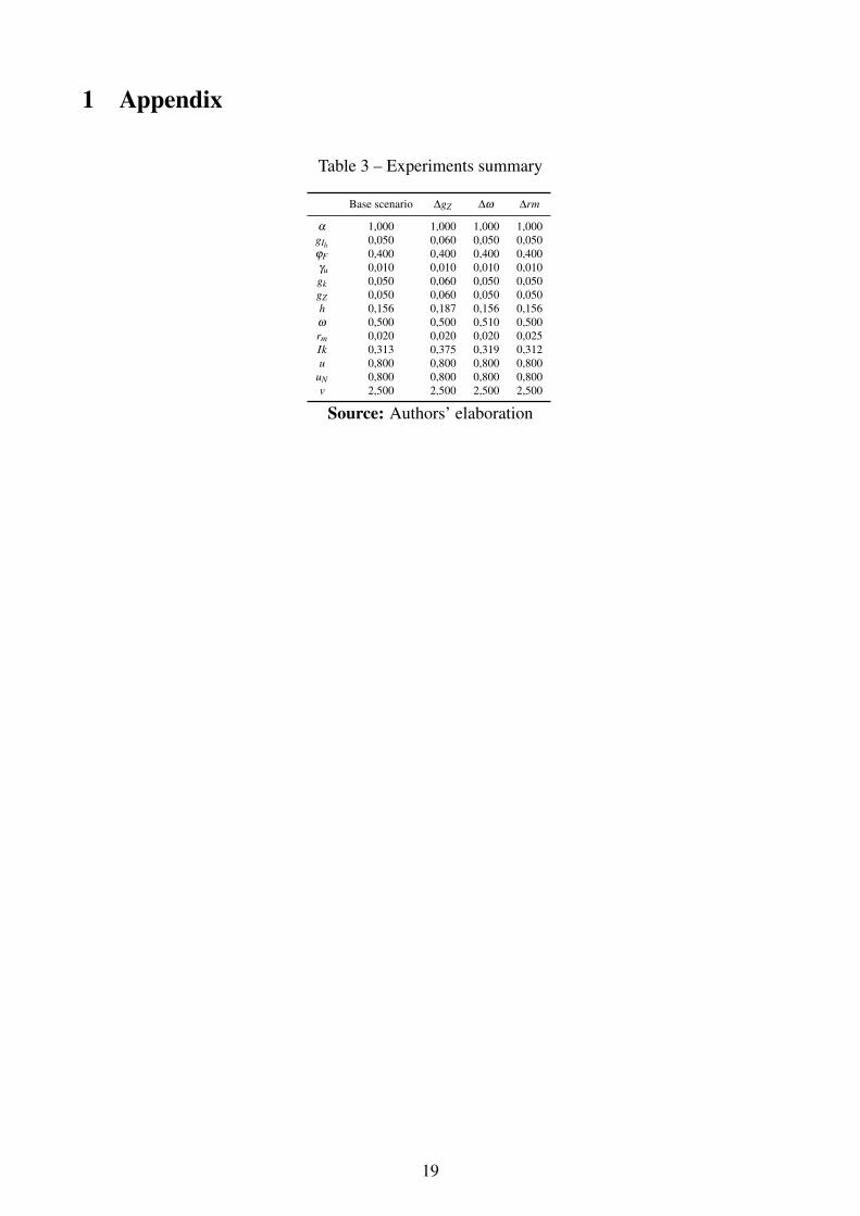
The remainder of this section presents the results of the following experiments: (i) increase ofresidential investment growth rate; (ii) wage share increase; (iii) increase of the interest rate. Theresults are summarized in appendix 1.

Increase of residential investment growth rate

An increase of of residential investment growth rate implies a greater growth rate of aggregate de-mand, therefore an increase of the degree of capacity utilization. Firms revise their investment plansaccordingly to capital stock adjustment principle and gradually increase their marginal propensity toinvest, causing output to temporarily grow faster than residential investment. The new full adjustedposition will be characterized by: a greater rate of growth of output, equal to the rate of growth of resi-dential investment; a greater investment share of output; and convergence towards the normal/planneddegree of capacity utilization.

Those results (figure 4) are in line with Sraffian Supermultiplier literature. The main distinctivecharacteristic of our model is the existence of two real assets. A result that can at first be consideredcounter intuitive is that a increase of residential investment growth rate causes a reduction of housingshare in total capital (i.e. an increase of k).

13

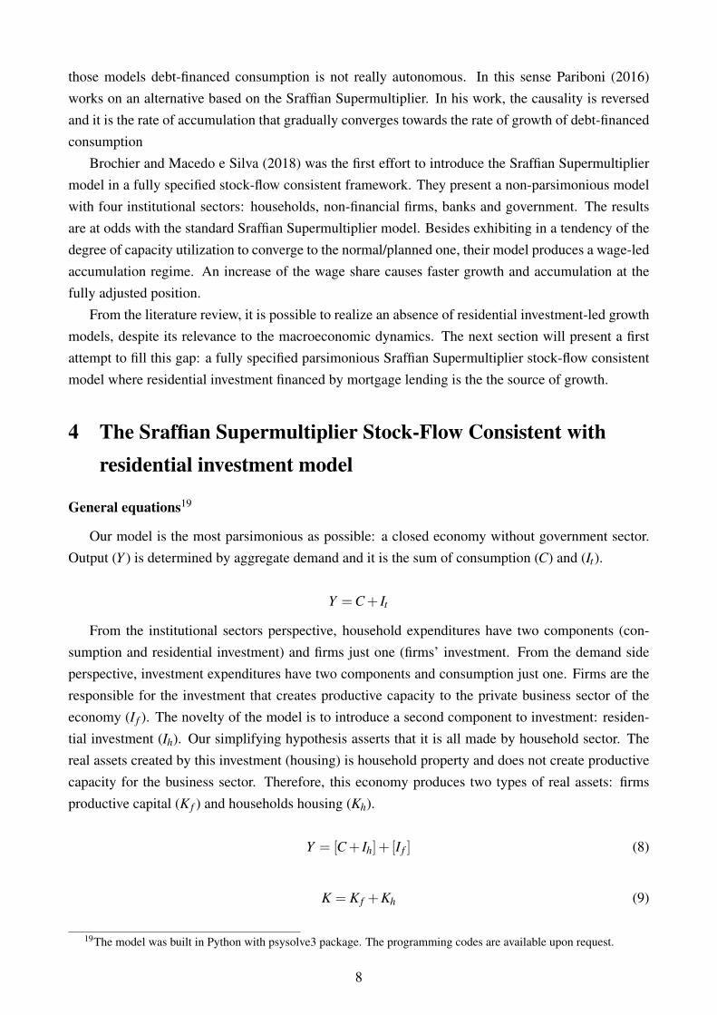
Increase of the wage share

The increase of the wage share increases the rate of growth of output and the degree of capacityutilization. But those effects are just temporarily, because the rate of growth of residential investmentdoes not change (figure 5). The main results are: marginal propensity to invest increases temporar-ily, and then returns to its baseline value; degree of capacity utilization quickly converges to thenormal/planned one.

Despite the effect on output growth rate being only temporary, this change has a permanent effecton firms capital share of total capital. The increase of the wage has a level effect on output and onoutput capacity, without affecting residential investment. The result is an increase of the share offirms capital in total real assets.

Increase of the rate of interest

An increase of the rate of interest does not have any effect on output growth, nor on the degreeof capacity utilization. The share of firms capital on total capital does not change, because thereis no change on distribution or the marginal propensity to invest. The only effect is a reductionof households savings due to payments of interest on mortgages increasing more than interests ondeposits received. The result is a greater compromise of disposable income with interest payments24.There is no changes of the rest of long-term results.

Figure 4 – Effects of an increase of residential investment rate of growth

Source: Authors’ elaboration

5 Final remarks

In this paper we have built a model aiming to contribute to the Sraffian Supermultiplier growthmodel, taking in consideration recent efforts of embedding it in a SFC framework. The main distinc-

24This effects can be seen ih the following equation:

rm ·M−1− rmo ·MO−1

Y D

14

Figure 5 – Effects of an increase of wage share

Source: Authors’ elaboration

Figure 6 – Effects of an increase of of interest rate

Source: Authors’ elaboration

tive characteristic of our model is putting residential investment as the driver of growth. The choiceof this specific expenditure is due to recent empirical works showing the relevance of dwelling ex-penditures for macroeconomic dynamics, as seen in section 2. Section 3 shows that we could not findany work that incorporated this feature in a demand-led growth model.

As expected, our model presents the main results of Sraffian Supermultiplier growth models:convergence towards normal/planned degree of capacity utilization is achieved by means of changesof marginal propensity to invest; and steady state output growth rate is determined by the rate ofgrowth of autonomous expenditures — in this case, residential investment. The main distinction ofour model is that there are two different kinds of real assets: firms capital and housing.

The experiments show that an increase of residential investment growth rate results in a smallerhousing share in total capital. Although seemingly counter intuitive, this result is a consequence ofcapital stock adjustment principle. Firms investment must temporarily grows faster than residential in-vestment in order for the actual degree of capacity utilization to converge towards the normal/plannedone. This is the cause of changes in the share of firms capital in total capital.

The other two experiments reports the results expected for Sraffian Supermultiplier growth mod-

15

els. An increase of wage share only has level effect on output and on capacity output. But preciselybecause of this level effect on capacity output, firms capital share in total capital increases. An in-crease of interest rate has only the effect of increasing firms debt-disposable income ratio.

It is important highlighting that this is just the first step of a wider research agenda on the role ofresidential investment for economic growth and business cycles. Future research should increase thedegree of complexity of this model. Some possible improvements of this model include: exploringthe determinants of residential investment to connect housing bubbles with aggregate demand and theinclusion of debt-financed consumption.

References

ALLAIN, O. Tackling the instability of growth: a Kaleckian-Harrodian model with an autonomousexpenditure component. en. Cambridge Journal of Economics, vol. 39, no. 5, pp. 1351–1371, Sept.2015.

BARBA, A.; PIVETTI, M. Rising household debt: Its causes and macroeconomic implications - Along-period analysis. Cambridge Journal of Economics, 2009.

BHADURI, A.; MARGLIN, S. Unemployment and the Real Wage: The Economic Basis for ContestingPolitical Ideologies. Cambridge Journal of Economics, vol. 14, no. 4, pp. 375–93, 1990.

BORTIS, H. Institutions, Behaviour and Economic Theory: A Contribution to Classical-KeynesianPolitical Economy. Cambridge England ; New York: Cambridge University Press, Nov. 1997.

BRAGA, J. Investment Rate, Growth and Accelerator Effect in the Supermultiplier Model: thecase of Brazil. 2018.

BROCHIER, L.; MACEDO E SILVA, A. C. A supermultiplier Stock-Flow Consistent model: the “re-turn” of the paradoxes of thrift and costs in the long run? en. Cambridge Journal of Economics,2018.

CESARATTO, S. Neo-Kaleckian and Sraffian Controversies on the Theory of Accumulation. en. Re-view of Political Economy, vol. 27, no. 2, pp. 154–182, Apr. 2015.

DEJUÁN, Ó. Hidden links in the warranted rate of growth: the supermultiplier way out. en. TheEuropean Journal of the History of Economic Thought, vol. 24, no. 2, pp. 369–394, Mar. 2017.

DOS SANTOS, C. H.; MACEDO E SILVA, A. C. Revisiting ’New Cambridge’: The Three FinancialBalances in a General Stock-Flow Consistent Applied Modeling Strategy. en. SSRN Electronic Jour-nal, 2010.

DUTT, A. K. Stagnation, income distribution and monopoly power. Cambridge Journal of Eco-nomics, vol. 8, pp. 25–40, 1984.

16

DUTT, A. K. Maturity, stagnation and consumer debt: a steindlian approach. en. Metroeconomica,vol. 57, no. 3, pp. 339–364, July 2006.

FAGUNDES, L.; FREITAS, F. The Role of Autonomous Non-Capacity Creating Expenditures in Re-cent Kaleckian Growth Models: an Assessment from the Perspective of the Sraffian SupermultiplierModel. en. In: ANAIS do X Encontro Internacional da Associação Keynesiana Brasileira. Brasília,2017. p. 24.

FIEBIGER, B. Semi-autonomous household expenditures as the causa causans of postwar US businesscycles: the stability and instability of Luxemburg-type external markets. en. Cambridge Journal ofEconomics, vol. 42, no. 1, pp. 155–175, Jan. 2018.

FIEBIGER, B.; LAVOIE, M. Trend and business cycles with external markets: Non-capacity generatingsemi-autonomous expenditures and effective demand. en. Metroeconomica.

FREITAS, F.; DWECK, E. The Pattern of Economic Growth of the Brazilian Economy 1970–2005: ADemand-Led Growth Perspective. In: LEVRERO, E. S.; PALUMBO, A.; STIRATI, A. (Eds.). Sraffaand the Reconstruction of Economic Theory: Volume Two: Aggregate Demand, Policy Analysisand Growth. London: Palgrave Macmillan UK, 2013. pp. 158–191.

FREITAS, F.; SERRANO, F. Growth Rate and Level Effects, the Stability of the Adjustment of Ca-pacity to Demand and the Sraffian Supermultiplier. en. Review of Political Economy, vol. 27, no. 3,pp. 258–281, July 2015.

GIRARDI, D.; PARIBONI, R. Long-run Effective Demand in the US Economy: An Empirical Test ofthe Sraffian Supermultiplier Model. en. Review of Political Economy, vol. 28, no. 4, pp. 523–544,Oct. 2016.

. Autonomous Demand and the Investment Share. 2018.

HARROD, R. F. An Essay in Dynamic Theory. en. The Economic Journal, vol. 49, no. 193, p. 14,Mar. 1939.

HEIN, E. Finance-Dominated Capitalism, Re-Distribution, Household Debt and Financial Fragilityin a Kaleckian Distribution and Growth Model. en. Rochester, NY, Jan. 2012.

JORDÀ, Ò.; SCHULARICK, M.; TAYLOR, A. M. The Great Mortgaging: Housing Finance, Crises,and Business Cycles. Sept. 2014.

KALDOR, N. Alternative Theories of Distribution. en. The Review of Economic Studies, vol. 23,no. 2, p. 83, 1955-56.

. A Model of Economic Growth. The Economic Journal, vol. 67, no. 268, pp. 591–624,1957.

KALECKI, M. Theory of economic dynamics. Routledge, 1954.

. Class struggle and the distribution of national income. en. Kyklos, vol. 24, no. 1, pp. 1–9,Feb. 1971.

KEYNES, J. M. The general theory of employment, interest, and money. New York/London: Har-court Brace Jovanavich, 1936.

17

LEAMER, E. E. Housing IS the Business Cycle. Sept. 2007.

NAH, W. J.; LAVOIE, M. Long-run convergence in a neo-Kaleckian open-economy model with au-tonomous export growth. Journal of Post Keynesian Economics, vol. 40, no. 2, pp. 223–238, Apr.2017.

PALLEY, T. Inside Debt and Economic Growth: A Neo-Kaleckian Analysis. In: HANDBOOK of Al-ternative Theories of Economic Growth. Edward Elgar Publishing, 2010. pp. 293–308.

PARIBONI, R. Household Consumer Debt, Endogenous Money and Growth: A Supermultiplier-Based Analysis. en. Rochester, NY, Sept. 2016.

PASINETTI, L. L. Rate of Profit and Income Distribution in Relation to the Rate of Economic Growth.Review of Economic Studies, vol. 29, no. 4, pp. 267–279, 1962.

ROBINSON, J. A model of accumulation. In: ESSAYS in the Theory of Economic Growth. 1. ed.London: Palgrave Macmillan UK, 1962.

ROWTHORN, B. Demand, Real Wages and Economic Growth. Thames Polytechnics, 1981.

SERRANO, F. Teoria dos Preços de Produção e o Princípio da demanda Efetiva. 1988. Dissertação(Mestrado) – Universidade Federal do Rio de Janeiro.

. LONG PERIOD EFFECTIVE DEMAND AND THE SRAFFIAN SUPERMULTIPLIER.en. Contributions to Political Economy, vol. 14, no. 1, pp. 67–90, 1995.

. The sraffian supermultiplier. 1995. Tese (PhD) – University of Cambridge, Cambridge.

SERRANO, F.; FREITAS, F. The Sraffian supermultiplier as an alternative closure for heterodox growththeory. en. European Journal of Economics and Economic Policies: Intervention, vol. 14, no. 1,pp. 70–91, 2017.

SERRANO, F.; FREITAS, F.; BEHRING, G. O Supermultiplicador Sraffiano, a Instabilidade Funda-mental de Harrod e o Dilema de Oxbridge, 2018. Mimeo.

SOLOW, R. M. A Contribution to the Theory of Economic Growth. en. The Quarterly Journal ofEconomics, vol. 70, no. 1, p. 65, Feb. 1956.

STEINDL, J. Maturity and Stagnation in American Capitalism. NYU Press, 1952.

. Stagnation theory and stagnation policy. en. Cambridge Journal of Economics, vol. 3,pp. 1–14, 1979.

TEIXEIRA, L. Uma Investigação sobre a desigualdade na distribuição de renda e o endividamento dostrabalhadores norte-americanos dos anos 1980 aos anos 2000. pt-BR. http://www.ipea.gov.br, Dec.2012.

. Crescimento liderado pela demanda na economia norte-americana nos anos 2000:uma análise a partir do supermultiplicador sraffiano com inflação de ativos. 2015. Tese (Doutorado)– Universidade Federal do Rio de Janeiro, Rio de Janeiro.

ZEZZA, G. U.S. growth, the housing market, and the distribution of income. Journal of Post Keyne-sian Economics, vol. 30, no. 3, pp. 375–401, Apr. 2008.

18

1 Appendix

Table 3 – Experiments summary

Base scenario ∆gZ ∆ω ∆rm

α 1,000 1,000 1,000 1,000gIh 0,050 0,060 0,050 0,050ϕF 0,400 0,400 0,400 0,400γu 0,010 0,010 0,010 0,010gk 0,050 0,060 0,050 0,050gZ 0,050 0,060 0,050 0,050h 0,156 0,187 0,156 0,156ω 0,500 0,500 0,510 0,500rm 0,020 0,020 0,020 0,025Ik 0,313 0,375 0,319 0,312u 0,800 0,800 0,800 0,800

uN 0,800 0,800 0,800 0,800v 2,500 2,500 2,500 2,500

Source: Authors’ elaboration

19